1  

The limits of selection under plant domestication

Robin G Allaby1* ,Dorian Q Fuller2, James L Kitchen1, 3

1. School of Life Sciences, Gibbet Hill Campus, University of Warwick,

Coventry CV4 7AL

2. Institute of Archaeology, University College London, 31-34 Gordon Square,

London WC1H 0PY

3. Computational and Systems Biology, Rothamsted, Harpenden, Herts.

* corresponding author email: r.g.allaby@warwick.ac.uk

  2  

Abstract

Plant domestication involved a process of selection through human agency of a series

of traits collectively termed the domestication syndrome. Current debate concerns the

pace at which domesticated plants emerged from cultivated wild populations and how

many genes were involved. Here we present simulations that test how many genes

could have been involved by considering the cost of selection. We demonstrate the

selection load that can be endured by populations increases with decreasing selection

coefficients and greater numbers of loci down to values of about s = 0.005, causing a

driving force that increases the number of loci under selection. As the number of loci

under selection increases, an effect of co-selection increases resulting in individual

unlinked loci being fixed more rapidly in out-crossing populations, representing a

second driving force to increase the number of loci under selection. In inbreeding

systems co-selection results in interference and reduced rates of fixation but does not

reduce the size of the selection load that can be endured. These driving forces result in

an optimum pace of genome evolution in which 50-100 loci are the most that could be

under selection in a cultivation regime. Furthermore, the simulations do not preclude

the existence of selective sweeps but demonstrate that they come at a cost of the

selection load that can be endured and consequently a reduction of the capacity of

plants to adapt to new environments, which may contribute to the explanation of why

selective sweeps have been so rarely detected in genome studies.

  3  

Introduction

Domestication is an evolutionary process that provides a cornerstone to understanding

the mechanism of selection (Darwin 1859). In the case of plants the evolution of

domestication involves the selection of a characteristic group of traits that are

collectively termed the domestication syndrome (Harlan et al. 1973, Hammer 1984).

These traits include the loss of shattering, changes in seed size, loss of photoperiod

sensitivity and changes in plant and spikelet architecture (Fuller 2007). It is

interesting that among crops of a similar type such as cereals, the number of

syndrome traits is also similar. It is not known whether this represents the maximum

number of traits that could have been selected within the time period of syndrome

fixation spanning several thousand years, or whether further traits could have been

selected in each case but were not. There has been much debate about how these traits

were selected, the pace and strength of selection, and the extent to which evolution

under domestication continues today (Fuller 2007, Brown et al. 2009, Honne & Heun

2009, Purugganan and Fuller 2009, Allaby et al. 2010, Abbo et al. 2010, 2011, Fuller

et al. 2011).

Classic field trials of experimental harvesting of wild progenitors of wheat

suggested that in the case of cereals selection coefficients as high as 0.6 could have

been in operation during domestication resulting in fixation of loss of shattering traits

within a few decades (Hillman And Davies 1990). These findings have been

supportive of a rapid transition model of agricultural origins (Diamond 2002) in

which domesticated forms of crops appeared over a very short time period in a

‘Neolithic Revolution’ (Zohary and Hopf 2000). However, an emergent feature of the

archaeological record in recent years has been the protracted appearance of

domesticated crops (Asouti and Fuller 2013, Tanno and Willcox 2006, 2012, Weiss et

  4  

al. 2006, Willcox 2005, Willcox et al. 2008, Willcox and Stordeur 2012, Hillman et al

2001) and estimates of selection coefficients made directly from the archaeobotanical

record have been as low as 0.003 (Purugganan and Fuller 2011, Fuller et al. 2014).

Under a protracted scenario of domestication, the expected patterns of genetic

diversity need to be re-evaluated in order to interpret the evolutionary history of

domestication (Allaby et al. 2008, Allaby 2010). For instance, under protraction traits

may have been selected more slowly in the face of gene flow between cultivated and

wild populations resulting in the appearance of relatively weak selection coefficients.

This extended time period would increase the opportunities for parallelisms in

syndrome traits as similar traits are independently selected in distinct geographic

locations, and genomic mosaicism associated with phylogeography could result

(Allaby 2010). It could also be the case that the protracted process allowed more

traits to be selected than would have been possible under the restricted time period of

a rapid transition of a few tens to hundreds of years. It is therefore useful to establish

how much selection would have been possible to drive the evolution of the

domestication syndrome under protracted and rapid transition scenarios.

Selection comes at a cost in that some organisms must die before reproducing

each generation for their genes to be selected against, so causing a reduction in the

overall population size. A consequence of this cost is that the amount of selection that

a species can withstand is limited. Haldane noted that for this reason there is a limit to

the number of traits that plant breeders are able to select at a given time, and that the

pace at which evolution can be driven by natural selection is limited because of the

cost of selection (Haldane 1957). In order to understand the pace of selection of the

domestication syndrome traits it is necessary to know the number of genetic loci

involved. Increasingly, the underlying genetic bases of the domestication syndrome

  5  

are being elucidated (Fuller and Allaby 2009), and the number of loci associated with

their control has recently been estimated to be 27, and as much as 70 in tetraploid

wheats (Peleg et al. 2011, Peng et al. 2003). Estimates of loci under selection from

the genome analysis of other crops have yielded a range of numbers, with up to 1200

loci suggested in maize, but an expectation of around 40 at the signal strength of tb1

(Wright et al. 2005) and 36 loci in sunflower (Chapman et al. 2008). The power to

detect signatures of selection in genetic data is limited (Yi et al 2010), so it is unclear

from these studies whether these numbers of loci under selection represent the totality

of loci or simply the most strongly selected loci that reach the threshold of

detectability. These numbers are high relative to the typical number of syndrome traits

because some traits, such as seed size, are under polygenic control (Gupta et al.

2006), while other traits, such as loss of shattering, are under the control of one or just

a few genes (Konishi et al. 2006, Li et al. 2006, Li & Gill 2006, Takahashi et al.

1955, Ishikawa et al 2010; Ishii et al 2013). Intuitively, it seems likely that traits under

monogenic control may be subject to stronger selection pressures than those under

polygenic control because the selection coefficients associated with each locus for a

trait have an additive effect. Therefore, as loci governing a trait are progressively

added, the value of s for each locus must progressively reduce in order to maintain the

same overall selection pressure on the individual organism. Consequently, it might be

expected that those traits of the domestication syndrome that are under monogenic

control would have been under the strongest selection and appeared the earliest.

Surprisingly, the reverse is observed in the archaeological record in that the tough

rachis mutant appears to be selected slowly and late relative to other traits (Tanno and

Willcox 2006, Fuller 2007), and increase in seed size appears very early on in the

archaeological record despite the complexity of its genetic control and a rate of

  6  

selection that is not significantly less than for shattering (Purugganan and Fuller 2011,

Fuller et al. 2014). While the timing of the first appearance of traits is attributable to a

sequence of different behaviors of proto-farmers subjecting different selection

pressures on plants at different times (Fuller et al. 2010, 2011), the surprising

similarity in rates highlights the need to better understand the selection pressures

involved in domestication.

In this study the limitations imposed by the cost of selection were examined

through computer simulations to establish the relationship between the number of loci

under selection, the strength of selection and the ability of plant populations to

recover from reduced population sizes resulting from rounds of selection. The

simulations were executed under a scenario based on the archaeological record in

which traits appear and are selected over a period of 3000 years (Fuller 2007, Fuller et

al. 2014, Tanno and Willcox 2006, 2012). Populations of virtual plants were endowed

with a number of loci, which were considered unlinked to each other and inherited

through a process of random segregation. In reality the overwhelming majority of

domestication syndrome loci have been identified to be regulatory in nature

(Purugganan and Fuller 2009, Meyer and Purugganan 2013). Consequently, it can be

inferred that most mutations have been epistatic in their effect. One can consider the

changes in gene expression caused by mutation at a distal regulatory locus to be a

phenotypic consequence, and that the focus of selection would act on the regulatory

locus rather than the regulated locus. Such a situation can be reasonably modeled by

treating each locus under selection as independent to other loci. This model makes no

assumption about the function of the loci under selection, and so the stage of the life

cycle in which the resultant phenotype is expressed, and is inclusive of epistatic

mutations. Furthermore, phenotypic traits may be under monogenic or polygenic

  7  

control. A model of independent selection of loci inherently describes traits under

monogenic control. Traits under polygenic loci are also described if it is assumed that

the overall trait, such as seed size, is contributed to by independently segregating loci,

which is largely true for quantitative traits. One might also consider that the selective

value of a mutation at a locus is dependent on the presence of mutations at other loci.

However, this would require a specific knowledge of the dependencies, which would

preclude a general model. Finally, it is known that some domestication syndrome loci

are located in close proximity to each other (Gepts 2004), and that positively selected

mutations may be associated with either linked deleterious loci, or have slightly

deleterious pleiotropic effects (Bomblies and Doebley 2006). In the case of tightly

linked loci, it is reasonable to model a single locus and the associated selection

coefficient thereby represents an overall selective value. The general effect of linkage

disequilibrium can reasonably be explored with a model of independently segregating

loci by including both inbreeding and outbreeding mating systems in which linkage

disequilibrium will be high and low respectively.

Given the assumptions outlined, it is reasonable to use a general model of

mutation selection of independently segregating loci in order to assess the amount of

selection that a plant population can endure under domestication. Each locus was

associated with a selection coefficient (s), which selected against the wild type allele.

Mutants were generated for loci in the population that had a fitness value of 1, so they

were not selected against. Individuals survived with a probability equal to the product

of the fitness values of alleles across all loci. Under this system, the resulting

individuals in the next generation would be fewer than the previous generation. The

ability of the population to recover from such a round of selection was determined by

a maximum fecundity parameter where each individual was capable of having more

  8  

than one progeny, causing the population to expand. However, population expansion

was tempered by both environmental checks and an environmental carrying capacity.

Therefore the number of individuals generated in the next generation was expanded

from the current generation value by an amount determined by the maximum

fecundity parameter (mf) up to the carrying capacity population size that could not be

exceeded. For each set of simulation conditions the probability of extinction, severity

of selection bottleneck, and the rate and extent of fixation of domestication syndrome

trait controlling alleles were determined.

It is well known that the rate of fixation of a mutation may be slowed down by

gene flow from an adjacent environment in which the same selection regime does not

apply. This is true in the case of the domestication syndrome in which the wild and

cultivated environments provide diametrically opposed selective forces on several

traits (Allaby 2010). The consequence of such gene flow is to reduce the proportion of

the advantageous mutant so in effect to reduce its selective advantage, and therefore

also the resulting selection coefficient between the mutant and the wild type. In an

explicit model gene flow would therefore effectively reduce the selection coefficient

from the input value making it an unknown parameter, which is undesirable in this

case. The cost of selection is correspondingly reduced as each wild type individual in

the local population that fails to reproduce is offset to some extent by immigrant wild

types. It is therefore a reasonable simplification to exclude gene flow from the model

in this case and consider the selection coefficients applied as comparable to the

resultant selection coefficient in the face of gene flow in terms of how the cost of

selection is limiting. The replenishment of the population through migration-mediated

gene flow (as opposed to purely pollen flow) is assumed to be negligible, and the

  9  

prevention of population extinction by the continual arrival of a few individuals not

carrying adaptive mutations is a largely uninformative parameter.

Results and Discussion

The maximum number of loci under selection. In the first set of simulation

experiments a model in which increasing numbers of loci subject to the same

selection coefficient was applied. Two regimes were considered relating to the ability

of members of the population to reproduce. The first was a conservative regime in

which there was an underlying assumption that the organisms were held in close

check by organisms of different species in the environment, close to Darwin’s original

insight that the typically geometric potential for species to reproduce is held back by

complex interspecific competition. Under this regime the mf parameter was set to 1.5,

such that a population was capable of expanding 50% at most per generation. The

second regime was considerably more liberal and mf was set to 10, allowing a ten-fold

expansion. The underlying rationale in this case was that a cultivated environment

inherently reduces interspecific competition, excepting that which is due to human

predation. The extent to which a crop population can expand is a function of the

number of propagules generated per plant, and the proportion of the harvest that is set

aside for sowing the following year. Previous studies have suggested that a quarter of

a crop harvest may be set aside representing about an eighth of the propagules

generated in a generation as it was estimated that approximately 50% of seeds were

harvested, with the rest lost due to dispersal and not sown (Hillman and Davies 1990).

Under such a regime an eightfold increase per individual would maintain an overall

constant population size, or an mf value of 1. However, cereals such as barley have up

  10  

20 or 30 grains per plant, which would lead to a 3-4 fold increase in population size

per generation under these conditions. In reality it is likely that a lower proportion of

the grain would be sown to compensate bringing the mf parameter to something close

to our conservative regime, however we selected an mf value of 10 to explore the

possible effect that could be introduced by human agency. We consider an mf of 10 to

be in excess of what is likely to be achieved.

Simulations were carried out on populations that began with 1000 individuals to

reflect a reasonable size based on genetic diversity studies (Zhu et al. 2007, Eyre-

Walker & Gaut 2007), but it should also be remembered that the pace of selection for

a given allele under a given selection coefficient is expected to be independent of

population size (Haldane 1924). This should not be confused with the parameter of

selection intensity (2Nes) often used in coalescent approaches that describes the

impact of selection on genetic diversity (Innan and Kim 2004), which is dependent on

population size. Each set of parameters were repeated 100 times. The two fecundity

regimes were explored using two mating systems, a 2% inbreeding population, similar

to that of wheat or barley, and a 98% out-crossing population to represent out-

crossing crops (tables S1-4). These mating systems represent the normal biases

expected in plants (Vogler and Kalisz 2001). The simulation outputs were used to

construct probability of survival landscapes under the four possible regimes, Figure 1.

It is notable that in all simulation parameters explored, the switch from survival to

extinction with increasing loci number under selection is precipitous, with populations

going from an estimated probability of survival of one to zero with the addition of just

1-5 loci in most cases. This change is more abrupt in out-crossing populations than

inbreeding ones. Generally, very few loci could be simultaneously under selection at

selection coefficients of 0.1 or higher, and values of s higher than 0.3 were unlikely to

  11  

be survived by populations under the conservative mf regime. We found that 80 and

83 were the maximum number of loci that could be selected under the conservative

expansion regime before extinction occurred under the lowest value of s explored

(0.005). This value is close to typical values under natural selection, and that

calculated from cereals in the archaeological record (Purugganan and Fuller 2011,

Fuller et al. 2014). Under the higher mf regime we found that 227 and 230 loci could

be under selection in out-crossing and inbreeding systems respectively at the lowest

value of s explored (0.01).

The probability of survival became less than one in populations that generally

experienced bottlenecks of less than 30% and less than 10% at the lower values of s.

While bottlenecks of this extremity may be found in nature, it is unlikely that such a

bottleneck could be tolerated under a cultivation regime since the majority of the food

source would disappear. We constructed landscapes to view the effect of selection on

bottleneck size, Figure 2. A precipitous drop is still discernible under the conserved

mf regime, which occurs at a threshold point when the bottleneck size is between 60

and 70% of the initial population size. In the case of the higher mf regime there is a

steady decline in bottleneck size. We judge that a reasonable level of bottleneck that

could be tolerated by cultivators is 60-70% before there is too great a reduction in

food production for it to be worthwhile investing in cultivation. Interestingly, all

regimes explored suggest that the number of loci that could be under selection for

such a bottleneck lie within the range of 50-100 loci (figure S1). This result is

particularly interesting because it closely mirrors the number of loci under selection

identified in genome studies of major crops (Peleg et al. 2011, Peng et al. 2003,

Wright et al. 2005, Chapman et al. 2008).

  12  

Selection from standing variation. The simulations so far consider mutants that occur

in very low frequencies in wild populations that are generally selected against in the

wild. A number of regulatory genes have been identified in maize that have been

selected during domestication which occur in a wide range of frequencies (0.1-0.88)

in the wild progenitor (Weber et al 2007, Studer et al 2011). In these sorts of cases it

is not expected that the wild and cultivated populations are subject to diametrically

opposed selection regimes, but instead aspects of adaptations to the wild environment

or neutral standing variation have selective value in the cultivated environment.

Models have shown that even strong selection will likely not leave a detectable

signature of selection from standing variation at higher frequencies (Innan and Kim

2004, Teshima et al 2006) because less of the adjacent genomic variation is lost

during the sweep process. Consequently, this part of the selection process during

domestication would be largely invisible from genome diversity scan approaches. To

investigate whether our estimates of the number of loci that could be under selection

were different from standing variation rather than spontaneous mutation, we carried

out simulations in which the starting frequency of the mutant was 0.5, Figure S2.

Generally, populations could sustain a larger number of loci under selection from

standing variation. Under these conditions there was a greater difference between the

mating strategies than for selection from spontaneous mutation. Outbreeding

populations sustained about 50% more loci before population extinction was

observed, whereas inbreeding populations sustained over 100% more loci. The

difference between the mating strategies is likely explained by the difference in

heterozygote proportions between the two population types. Inbreeding populations

hold most of the recessive mutations in homozygous individuals, which therefore

confer an advantage to the individual. The difference between selection from standing

  13  

variation and spontaneous mutation is less pronounced when the population

bottleneck is considered, Figure S3. The 60-70% threshold that we consider to be a

realistic pragmatic limit for cultivation is reached in the 50-110 loci range from

standing variation for weak selection (s = 0.005).

Co-selection and the interference between loci. In reality it is unlikely that all loci

would be under equal selection pressure. Therefore in the third set of experiments we

explored mixed selection regimes in which there was one strong selection pressure,

combined with varying numbers of weakly selected loci. In this case we selected a

value of 0.3 for s to represent strong selection, and 0.01 for s to represent relatively

weak selection. In this set of experiments we only considered the conservative

fecundity regime in which mf was set at 1.5.

In a mixed regime the maximum number of weak loci that could be added to the

strongly selected loci before extinctions occurred was 6 and 4 for the inbreeding and

out-crossing regimes respectively (table S5). The total amount of selection that a

population is subject to can be expressed by a ‘selection load’, which we define as the

sum of the selection coefficients of the loci under selection. In this mixed regime a

selection load of 0.34-0.36 was endured by populations, which is less than that

endured by populations subjected to selection at s set to 0.01 only (0.4-0.41). A

notable effect was that rate at which advantageous mutants of loci subject to strong

selection were fixed increased in the presence of selection of increasing numbers of

weakly selected loci, but the effect is not clearly apparent in the weakly selected loci,

Figure 3. Since loci were unlinked, the rate increase is unlikely to be due to a

hitchhiking effect. Previously, it has been suggested that an additive selective

advantage effect could occur in individuals that received mutants with adaptive values

  14  

to two unrelated selection regimes from different source populations, resulting in a

type of cultivation magnetism between the two source populations (Allaby 2010). An

alternative explanation that might be forwarded is that the reduced population size in

the bottleneck caused by the increased selection load of many weakly selected loci

may increase the rate at which the strongly selected loci are fixed, although we do not

expect this to be the case from previous theory (Haldane 1924). To distinguish

between these possibilities we carried out a set of simulations on just the one strongly

selected locus in smaller populations that closely matched bottleneck sizes in the

mixed selection regimes. In the case of the out-crossing population a size of 500

individuals was selected, which closely matches the bottleneck of the mixed regime

with 5 weakly selected loci, and a size of 300 was selected for the inbreeding

population, which closely matches the mixed regime with 10 weakly selected loci. In

both cases the smaller population size did not produce fixation rates as fast as with the

mixed regime, showing that the additive effect of loci is a more likely cause than

reduced population size.

The interference in the rate of selection caused by co-selection was investigated

further by plotting the rate of fixation of increasing numbers of loci under uniform

regimes of either strong or weak selection, Figure 4. Under these conditions the

additive advantage occurred in out-crossing populations, but increased loci burden led

to a decrease in the rate of fixation of inbreeding populations. This result can be

explained by the mating strategy. The rate at which advantageous mutations are

united in single individuals by crossing is lower in an inbreeding system than in an

out-crossing one. Consequently, in an inbreeding system although an individual may

have a single advantageous mutation, it will have numerous disadvantageous alleles at

other loci that will depress its probability of success. The result is that the numerous

  15  

loci will interfere with each other to an extent dependent on the number of loci

involved. This effect of mating system is similar to the Hill-Robertson effect noted in

Oryza (Hill-Robertson 1974, Flowers et al. 2012) in which diversity is depressed in

inbreeders, although the loci are physically unlinked in this model demonstrating that

mating system alone is highly influential as well as genome location for interference

of selection of loci. The exception in this study is when a strongly selected locus is in

the presence of weakly selected loci in an inbreeding population. In this case it

appears that the depressing effects of the weak loci have little effect on the strongly

selected locus, but the locus does benefit from the additive effect of recruiting weakly

advantageous mutations.

The out-crossing populations show a less complex pattern in co-selection

effects. In both weakly and strongly selected loci, an increase in loci number increases

the rate at which each locus is fixed. In the case of weakly selected loci, the number

of loci has to be relatively large before the effect becomes clear. The effects of co-

selection suggest that any particular trait will be selected for more quickly in the

presence of a second, unrelated, selection pressure acting on an unlinked locus.

Consequently, there appears to be a synergistic consequence to multiple unrelated

selection pressures that could drive an organism to adapt to new environments and

outcompete organisms adapting to fewer environments.

Selection load and an optimum pace of selection at the genomic level. The total

selection load that populations were subjected to without extinctions occurring

increased with decreasing selection pressure per locus, Table S6. This leads to an

interesting dynamic, because although more strongly selected loci are fixed more

quickly, the total amount of selection that can be endured at one time is less, which is

  16  

reminiscent of the tale of the tortoise and the hare. This demonstrates that an adaptive

regime over many loci can endure an environment which is more complex and overall

harsher than one in which a single mutant is acutely selected, therefore rendering such

complex harsher environments open to the ‘tortoise’ which would be unavailable to

the ‘hare’. Hares, on the other hand may be better suited to adapt acutely to extreme

environments of low complexity. It is also notable that populations under strong

selection pressures per locus are vulnerable to extinction at bottleneck sizes that are

considerably larger than in the case of weak selection pressures, for instance between

40 and 50% in the mixed selection regime (table S5), but only 14-15% under

comparable weak selection (tables S1 and S2). The hare strategy therefore is much

more risky, achieves less selection overall due to the risk of extinction and as a

consequence would likely produce populations that were ultimately weaker.

Ever decreasing levels of selection per locus will eventually lead to no selection

at all, which raises the question is there an optimum number of loci and level of

selection? The extent to which the survivable selection load increases with decreasing

selection per locus diminishes with the latter parameter (Figure S4). In the case of the

conservative reproductive regime where the mf parameter was set to 1.5, the selection

load would not be expected to be much greater than 0.41 observed at a level of

selection at which s is set to 0.005. Similarly, in our liberal reproductive regime there

may be a little improvement on the selective load of 2.3 observed by reducing s from

0.01 to 0.005. Therefore the advantage of an increased selective load is not likely to

be greatly improved at selection coefficients much below 0.005. It is perhaps for this

reason that the selection coefficients observed in nature tend to be of this order of

magnitude, and perhaps also one reason why apparently disparate selection regimes

on different domestication syndrome traits have yielded very similar measurements of

  17  

selection coefficients, also in this order of magnitude (Purugganan and Fuller 2011;

Fuller et al 2014).

We finally calculated the average maximum rate of substitution achieved under

each of our selection regimes without extinctions occurring (Figure S5). Generally, a

larger number of substitutions had been achieved per generation under the lower

selection regimes by the time all mutants would have been fixed. Haldane originally

estimated that one substitution every 300 generations corresponding to a selection

coefficient of 0.1 was about what could be expected of natural selection (Haldane

1957). Our models agree quite well with this estimation, and suggest that at lower

levels of selection across the genome, the pace could be considerably faster.

The pace of selection of the domestication syndrome in plants. The simulations in

this study demonstrate that regardless of the reproductive capacity of plants there is an

optimum level of selection across a plant genome in the order of s equal to 0.005 that

should apply to natural selection as well as selection in the cultivated environment.

Co-selection will tend to further push genome evolution towards a maximum number

of loci under selection in out-crossing species. Under cultivation there is likely to be a

stringent restriction on bottleneck size in order to maintain a viable food source, and

we estimate that as a result the expectation of the number of loci under selection

should be in the range of around 50-100 loci. This value is true of selection from

spontaneous mutants as well as from standing variation. These findings suggest that

genome wide efforts to detect signatures of selection in crops are probably recovering

most of the loci under selection, and that those loci were most likely selected from

spontaneous mutations since selection from standing variation is less likely to be

detected in genomic signatures. The difference between the number of signatures of

  18  

selection detected and the upper limits described here reflects the amount of selection

that could have occurred from standing variation. This suggests that domesticated

wheat was mostly based on spontaneous mutation, maize and sunflower may have had

progressively more of their domestication adaptations from standing variation.

Germane to this observation is that selection of recessive mutants is quicker in

inbreeding populations where the majority of individuals are homozygous through

selfing. Therefore, it would have been easier for the inbreeding crops such as wheat

and barley to select spontaneous mutation, while maize and sunflower would likely

have had a greater pressure to incorporate standing variation.

While these simulations do not preclude the existence of selective sweeps, they

do show that sweeps come at a cost of reducing the selection load that a population is

capable of enduring. This could explain why sweeps are rarely observed in nature, but

also why agricultural expansion was repeatedly associated with collapse in new

environments shortly after arrival (Shennan et al. 2013, Stevens and Fuller 2012). It is

possible that the rapid pace of expansion could have forced equally rapid adaptation

of plants to latitude, which would have required strong selection of a low number of

loci – an adaptation of low complexity. Given the dynamic complex environment into

which agriculture had advanced, it may have been the case the plant populations were

incapable of further adaptation to changing conditions as they occurred. To better

understand the expansion of agriculture further consideration is needed of the pace of

movement across the latitudinal selection gradient in the context of tolerable limits of

plants, and whether different paces are associated adaptations of low and high

complexity respectively (Kitchen and Allaby 2013).

Methods

  19  

The simulations were carried out using a program written by R.G.A. For the program

details and methodology, see SI Text. Simulations were carried with populations of

1000 individuals. The simulation begins with an initialization of the population in

which hermaphrodite individuals are assigned wild type alleles for the defined

number of loci under selection. A mutation rate of 0.001 was used, such that on

average a single recessive advantageous mutation would appear each generation in

populations that had no mutants. In subsequent generations, individuals were

generated by randomly selecting gametes (themselves generated through a process of

random segregation with all loci unlinked) from individuals of the previous

generation with a probability of selecting the same donor twice equal to the mating

strategy (0.02 for out-crossing simulations and 0.98 for inbreeding populations).

Newly generated individuals then survived with a probability equal to the product of

the fitness values of the alleles they carried, such that the probability of survival (su)

was defined as:

su = !i1

k

!         (1)

For k loci, where  ωI is the fitness of the ith locus as given by:

!i =1! si         (2)

Where si is the selection coefficient of the ith locus. The selection coefficient of the ith

locus was moderated by the value lambda for heterozygotes (Shet) such that

sihet = (1!!)si         (3)  

A value of 0 was taken for lambda in all simulations in this study to represent

recessive mutations, which represent the majority of known mutations associated with

domestication. In the first generation this step was repeated for a number of times

equal to the population size, and inevitably led to a number of individuals in the next

  20  

generation which were fewer than this value. In subsequent generations the number of

attempts at making new individuals was given by

Nattempts = Nn!1mf         (4)

For (Nattempts < initial population size), where Nattempts is the number of individuals

created then challenged, Nn-1 is the number of individuals in the previous generation

and mf is the maximum fecundity parameter. Where this condition was violated, the

initial population size was used, representing the carrying capacity of the

environment. This process was iterated for the specified number of generations.

Simulations were carried out for 3000 generations. Each set of simulation

conditions was repeated 100 times, and average frequencies of advantageous mutants

for each locus and population sizes were recorded for each generation. The number of

generations per substitution was calculated by dividing the time to fixation by the

number of loci that had been fixed under maximum selection load conditions for a

given value of s. Time to fixation (F) was approximated when fixation had been

incomplete at the end of simulations using a logistic sigmoid function equation (5).

! ≈   !".!!

!.!!!" !!!!

(5)

Where G is the number of generations in the simulation and f is the final

frequency of the mutant under selection.

Acknowledgements

This work was kindly supported by the Leverhulme Trust (grant number F/00

215/BC).

References

  21  

Abbo S, Lev-Yadun S, Gopher A (2010) Agricultural origins: centres and non-

centres: a Near Eastern reappraisal. Critical Reviews in Plant Sciences 29: 317–328.

Abbo S, Rachamim E, Zehavi Y, Zezak I, Lev-Yadun S, Gopher A (2010)

Experimental growing of wild pea in Israel and its bearing on Near Eastern plant

domestication. Annals of Botany 107: 1399–1404.

Abbo S, Lev-Yadun S, Gopher A (2011) Origin of Near Eastern plant domestication:

homage to Claude Levi-Strauss and ‘La Penseae Sauvage’. Genetic Resources and

Crop Evolution 58:175–179.

Allaby RG (2010) Integrating the processes in the evolutionary system of

domestication. Journal of Experimental Botany 61:935-944.

Allaby RG, Brown T, Fuller DQ (2010) A simulation of the effect of inbreeding on

crop domestication genetics with comments on the integration of archaeobotany and

genetics: a reply to Honne and Heun. Vegetation History and Archaeobotany 19:151–

158.

Allaby RG, Fuller DQ, Brown TA (2008) The genetic expectations of a protracted

model for the origins of domesticated crops. Proceedings of the National Academy of

Sciences USA 105:13982-13986.

Asouti, E and Fuller DQ (2013) A Contextual Approach to the Emergence of

Agriculture in Southwest Asia. Current Anthropology 54 (3): 299-345

  22  

Bomblies, K, Doebley JF (2006) Pleiotropic effects of the duplicate maize

FLORICAULA/LEAFY genes zfl1 and zfl2 on traits under selection during maize

domestication. Genetics 172:519–531

Brown TA, Jones MK, Powell W, Allaby RG (2009) The complex origins of

domesticated crops in the fertile crescent. Trends in Ecology and Evolution 24:103-

109.

Chapman et al. (2008) A genomic scan for selection reveals candidates for genes

involved in the evolution of cultivated sunflower (Helianthus annuus) Plant Cell

20:2931-2945.

Darwin C (1859) Variation under domestication. In: Origin of species. London:

Murray, 7–43.

Diamond J (2002) Evolution, consequences and future of plant and animal

domestication. Nature 418:700–707.

Eyre-Walker A, Gaut B (1998) Investigation of the bottleneck leading to the

domestication of maize. Proc Natl Acad Sci USA 95:4441–4446.

Flowers JM, Molina J, Rubinstein S, Huang P, Schaal BA, Purugganan M (2012)

Natural selection in gene dense regions shapes the genomic pattern of polymorphism

in wild and domesticated rice. Mol. Biol. Evol. 29:675-687.

  23  

Fuller 2007 Contrasting patterns in crop domestication and domestication rates: recent

archaeobotanical insights from the Old World. Ann Bot 100:903–909

Fuller DQ and Allaby RG (2009) Seed Dispersal and Crop Domestication: shattering,

germination and seasonality in evolution under cultivation in Fruit development and

Seed Dispersal, Annual Plant Reviews 38:238-295.

Fuller DQ, Denham T, Arroyo-Kalin M, Lucas L, Stephens C, Qin L, Allaby RG,

Purugganan MD (2014) Convergent evolution and parallelism in plant domestication

revealed by an expanding archaeological record. Proc. Natl. Acad. Sci. U.S.A.

doi/10.1073/pnas.1308937110

Fuller DQ, Allaby RG, Stevens C(2010) Domestication as innovation: the

entanglement of techniques, technology and chance in the domestication of cereal

crops.World Archaeology 42(1): 13-28

Fuller DQ, Willcox, G, Allaby RG (2011) Cultivation and domestication had multiple

origins: arguments against the core area hypothesis for the origins of agriculture in the

Near East. World Archaeology 43:628-652.

Gepts P (2004) Crop domestication as a long term selection experiment. Plant

Breeding Reviews 24:1–44.

  24  

Gupta P, Rustgi S, Kumar N (2006) Genetic and molecular basis of grain size and

grain number and its relevance to grain productivity in higher plants. Genome 49:

565-571.

Haldane JBS (1924) A mathematical theory of natural and artificial selection. Part I.

Transactions of the Cambridge Philosophical Society 23:3-41.

Haldane JBS (1957) The cost of selection. J. Genet. 55:511-524.

Hammer (1984) Das Domestikationssyndrom. Kulturpflanze 32:11–34

Harlan JR, de Wet JMJ, Price EG (1973) Comparative evolurtion of cereals.

Evolution 27:311-325.

Hill-Roberston W (1974) Estimation of linkage disequilibrium in randomly mating

populations. Heredity 33:229-239.

Hillman GC, Davies MS. 1990. Domestication rates in wild-type wheats and barley

under primitive cultivation. Biological Journal of the Linnean Society 39:39–78

Hillman GC, Hedges R, Moore AMT, Colledge S, Pettitt P (2001) New evidence of

Late Glacial cereal cultivation at Abu Hureyra on the Euphrates. The Holocene 11:

383–393.Honne BJ, Heun M (2009) On the domestication genetics of self fertilizing

plants. Vegetation History and Archaeobotany 18:269–272.

  25  

Innan H, Kim Y (2004) Pattern of polymorphism after strong artificial selection.

Proc. Natl. Acad. Sci. U.S.A. 101:10667-10672.

Ishikawa R, Thanh PT, Nimura N, Htun TM, Yamasaki M, Ishii T. (2010) Allelic

interaction at seed-shattering loci in the genetic backgrounds of wild and cultivated

rice species. Gene Genet Syst.85:265–71.

Ishii T, Numaguchi K, Miura K, Yoshida K, Thanh PT, Htun TM, Yamasaki M,

Komeda N, Matsumoto T, Terauchi R, Ishikawa R, Ashikari M (2013)

OsLG1 regulates a closed panicle trait in domesticated rice. Nature Genetics 45:462–

465

Kitchen JL and Allaby RG (2013) Systems Modeling at Multiple Levels of

Regulation: Linking Systems and Genetic Networks to Spatially Explicit Plant

Populations. Plants 2013, 2(1), 16-49.

Konishi et al. (2006) A SNP caused loss of seed shattering during rice domestication.

Science 312: 1392-1396

Li W, Gill BS (2006) Multiple genetic pathways for seed shattering in the grasses.

Functional and. Integrative Genomics 6: 300-309.

Li C, Zhou A, Sang T (2006) Rice domestication by reducing shattering. Science 311:

1936-1939.

  26  

Meyer RS, Purugganan MD (2013) Evolution of crop species: genetics of

domestication and diversification. Nature Reviews Genet. 14:840-852.

Peleg Z, Fahima T, Korol AB, Abbo S, Saranga Y (2011) The genetic basis of wheat

domestication and evolution under domestication. J. Exp. Bot. 62:5051-5061.

Peng J, Ronin Y, Fahima T, Röder MS, Li Y, Nevo E, Korol A (2003) Domestication

quantitative loci in Triticum dicoccoides, the progenitor of wheat. Proc. Natl. Acad.

Sci. USA 100:2489-2494.

Purugganan MD, Fuller DQ (2009) The nature of selection during plant

domestication. Nature 457:843–848.

Purugganan and Fuller (2011) Archaeological data reveal slow rates of evolution

during plant domestication. Evolution 65:171–183.

Shennan, S., Downey, S.S., Timpson, A., Edinborough, K., Kerig, T., Manning, K.,

Thomas, M.G. (2013) Regional population collapse followed iitial agricultural booms

in mid –Holocene Europe. Nat. Comms. 4, 2486.

Stephens, C.J. & Fuller, D.Q. (2012) Did Neolithic farming fail? The case for a

Bronze Age agricultural revolution in the British Isles. Antiquity 86, 707-722.

  27  

Studer A, Zhao Q, Ross-Ibarra J, Doebley J (2011) Identification of a functional

transposon insertion in the maize domestication gene tb1. Nature Genet. 43:1160-

1165.

Takahashi R (1955). The origin and evolution of cultivated barley. In Demerc, M.

(ed.) Advances in genetics 7. New York: Academic Press, 227-266.

Tanno K-I, Willcox G (2006) How fast was wild wheat domesticated? Science 311:

1886.

Tanno K-I, Willcox G (2012) Distinguishing wild and domestic wheat and barley

spikelets from early Holocene sites in the Near East. Vegetation History and

Archaeobotany 21:107–115.

Teshima KM, Coop G, Przeworski (2007) How reliable are empirical genomic scans

for selective sweeps. Genome Res. 16:702-716.

Vogler DW, Kalisz S (2001) Sex among the flowers: the distribution of plant mating

systems. Evolution 55: 202–204.

Weber A, Clark RM, Vaughn L, Sanchez-Gonzalez JJ, Yu J, Yandell BS, Bradbury P,

Doebley (2007) Major regulatory genes in maize contribute to standing variation in

teosinte (Zea mays ssp. parviglumis). Genetics 177:2349-2359.

  28  

Weiss E, Kislev ME, Hartmann A (2006) Autonomous cultivation before

domestication. Science 312:1608–1610.

Willcox G (2005) The distribution, natural habitats and the availability of wild cereals

in relation to their domestication in the Near East: multiple events, multiple centres.

Vegetation History and Archaeobotany 14: 534–541.

Willcox G, Fornite S, Herveux LH (2008) Early Holocene cultivation before

domestication in northern Syria. Vegetation History and Archaeobotany 17:313–325.

Willcox, G. & Stordeur, D. (2012) Large-scale cereal processing before domestication

during the tenth millennium cal BC in northern Syria. Antiquity 86, 99-114.

Wright S et al. (2005) The effects of artificial selection on the maize genome. Science

308:1310-1314

Yi X, Liang Y, Huerta-Sanchez E, Jin X, Cuo ZXP, Pool JE et al 2010 Sequencing of

50 Human Exomes reveals adaptation to high altitude. Science 329:75-78.

Zhu Q, Zheng X, Luo J, Gaut BS, Ge S (2007) Multilocus analysis of nucleotide

variation of Oryza sativa and its wild relatives: severe bottleneck during

domestication of rice. Mol. Biol. Evol. 24:875-888.

Zohary  D,  Hopf  M  (2000)  Domestication  of  plants  in  the  Old  World,  3rd  edn.  

Oxford:  Oxford  University  Press.  

  29  

  30  

Figure 1. Probability landscapes of population survival (p) for a given number of loci

(g) under selection coefficient (s). A. Inbreeding population with mf of 1.5. B. Out-

crossing population with mf of 1.5. C. Inbreeding population with mf of 10. D. Out-

crossing population with mf of 10.

Figure 2. Landscapes of minimum population bottleneck (b) expressed as a proportion

of original population size for a given number of loci (g) under selection coefficient

(s). See Figure 1 for conditions A – D.

Figure 3. Proportion of advantageous mutants in population (f) over time

(generations) under mixed selection regimes of a single locus selected with s of 0.3,

and varying numbers of loci selected with s of 0.01. A. Fixation of 0.3 selected locus

in the presence of 0,1,5 and 10 loci at 0.01, a 0.3 locus in an initial population of 500

individuals, and a single 0.31 locus (out-crossing). B. A 0.01 selected locus in the

presence of 0,1,5 and 10 other loci, one of which was selected at 0.3 and the others at

0.01 (out-crossing). C. A 0.3 selected locus in the presence of 0,1,5 and 10 loci at

0.01, a 0.3 locus in an initial population of 300 individuals, and a single 0.31 locus

(inbreeding). D. A 0.01 selected locus in the presence of 0,1,5 and 10 other loci, one

of which was selected at 0.3 and the others at 0.01 (inbreeding).

Figure 4. Proportion of advantageous mutants in population (f) over time

(generations) with increasing numbers of loci in a uniform selection regime. A. 0.3

selected loci (outbreeding). B 0.01 selected loci (outbreeding). C. 0.3 selected loci

(inbreeding). D. 0.01 selected loci (inbreeding).

  31  

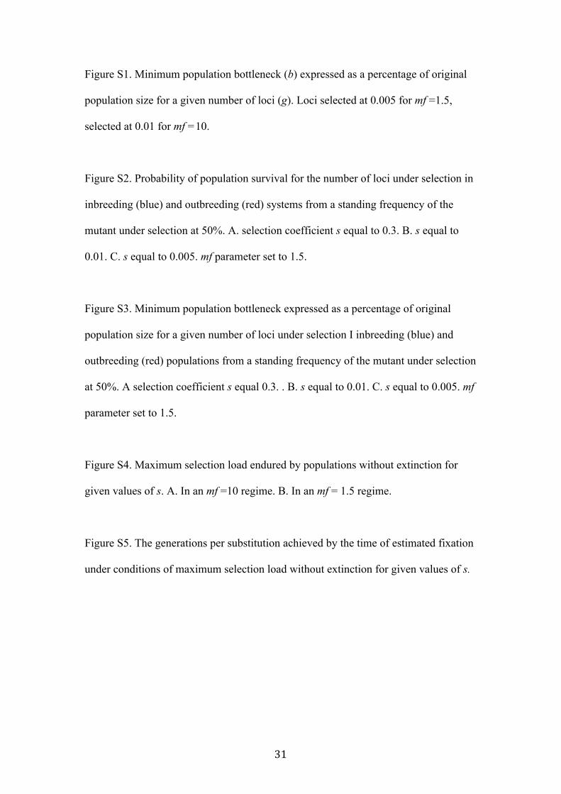
Figure S1. Minimum population bottleneck (b) expressed as a percentage of original

population size for a given number of loci (g). Loci selected at 0.005 for mf =1.5,

selected at 0.01 for mf =10.

Figure S2. Probability of population survival for the number of loci under selection in

inbreeding (blue) and outbreeding (red) systems from a standing frequency of the

mutant under selection at 50%. A. selection coefficient s equal to 0.3. B. s equal to

0.01. C. s equal to 0.005. mf parameter set to 1.5.

Figure S3. Minimum population bottleneck expressed as a percentage of original

population size for a given number of loci under selection I inbreeding (blue) and

outbreeding (red) populations from a standing frequency of the mutant under selection

at 50%. A selection coefficient s equal 0.3. . B. s equal to 0.01. C. s equal to 0.005. mf

parameter set to 1.5.

Figure S4. Maximum selection load endured by populations without extinction for

given values of s. A. In an mf =10 regime. B. In an mf = 1.5 regime.

Figure S5. The generations per substitution achieved by the time of estimated fixation

under conditions of maximum selection load without extinction for given values of s.

   

   

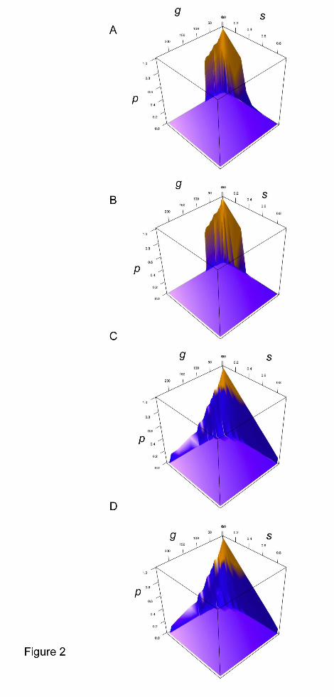
 Figure  S2  

!"!#$"!#%"!#&"!#'"!#("!#)"!#*"!#+"!#,"$"

!" $" %" &" '" (" )" *" +" ," $!" $$" $%" $&" $'"

!"#$

%$&'&()*#+*!

#!,'%-

#.*/,

"0&0%'*

.,1$2"*#+*'#3&*,.42"*/2'23-#.*

!"!#$"!#%"!#&"!#'"!#("!#)"!#*"!#+"!#,"$"

!" %!" '!" )!" +!" $!!" $%!" $'!" $)!"

!"#$

%$&'&()*#+*!

#!,'%-

#.*/,

"0&0%'*

.,1$2"*#+*'#3&*,.42"*/2'23-#.*

!"!#$"!#%"!#&"!#'"!#("!#)"!#*"!#+"!#,"$"

!" (!" $!!" $(!" %!!" %(!" &!!"

!"#$

%$&'&()*#+*!

#!,'%-

#.*/,

"0&0%'*

.,1$2"*#+*'#3&*,.42"*/2'23-#.*

A

B

C

                           

                             

                             

   Figure  S3  

!"

#!"

$!"

%!"

&!"

'!"

(!"

)!"

*!"

+!"

#!!"

!" #" $" %" &" '" (" )" *" +" #!" ##" #$" #%" #&" #'"

!"#$%&%

'()*"*

+$,-

"&)./0%)

123)

&+4!%5)"6)$"'/)+&7%5).%$%'-"&)

!"

#!"

$!"

%!"

&!"

'!"

(!"

)!"

*!"

+!"

#!!"

!" $!" &!" (!" *!" #!!" #$!" #&!"

!"#$%&%

'()*"*

+$,-

"&)./0%)

123)

&+4!%5)"6)$"'/)+&7%5).%$%'-"&)

!"

#!"

$!"

%!"

&!"

'!"

(!"

)!"

*!"

+!"

#!!"

!" '!" #!!" #'!" $!!" $'!"

!"#$%&%

'()*"*

+$,-

"&)./0%)

123)

&+4!%5)"6)$"'/)+&7%5).%$%'-"&)

A

B

C

                                                         Figure S4          

!"!#$"!#%"!#&"!#'"("

(#$"(#%"(#&"(#'"$"

$#$"$#%"

!" !#!)" !#(" !#()" !#$" !#$)" !#*"

+,(!"-./0112-.3"

+,(!"456/0112-.3"

!"

!#!$"

!#%"

!#%$"

!#&"

!#&$"

!#'"

!#'$"

!#("

!#($"

!" !#%" !#&" !#'"

)*"%#$"+,-.//0+,1"

)*"%#$"234-.//0+,1"

A

B

sl

sl

s

         

           

                 Figure S5  

!"#!!"$!!"%!!"&!!"

'!!!"'#!!"'$!!"'%!!"'&!!"#!!!"

!" !('" !(#" !()"

*+"'!",-./001,-2"

*+"'!"345./001,-2"

*+"'(6",-./001,-2"

*+"'(6"345./001,-2"

s

gens/sub

Table  S1.  Summary  of  simulation  outputs  for  out-­‐crossing  populations  with  mf  =  1.5

s loci  number %extinction %frequency %bottleneck

0.9 1 100 0 00.9 2 100 0 00.8 1 100 0 00.8 2 100 0 00.7 1 100 0 00.6 1 99 99 00.6 2 100 0 00.5 1 96 96 0.1250.5 2 100 0 00.4 1 90 90 1.7740.4 2 100 100 00.4 3 100 100 00.3 1 0 0 69.5250.3 2 98 98 0.4810.3 3 100 100 00.2 1 0 100 79.6340.2 2 81 100 3.9960.2 3 100 100 00.2 4 100 100 00.1 1 0 98 89.6960.1 2 0 98 80.5490.1 3 0 98 72.6460.1 4 42 99 12.8650.1 5 100 100 00.05 1 0 85 94.90.05 2 0 89 900.05 3 0 86 85.50.05 4 0 89 81.20.05 5 0 86 77.10.05 6 0 85 73.1080.05 7 0 86 69.5690.05 8 11 88 29.5230.05 10 100 0 00.04 1 0 75 95.80.04 2 0 79 91.80.04 3 0 77 88.20.04 4 0 81 84.70.04 5 0 79 81.30.04 10 7 84 34.0480.04 11 95 83 0.33

0.04 12 100 0 00.03 1 0 75 96.70.03 2 0 70 93.80.03 3 0 72 910.03 4 0 72 88.240.03 5 0 73 85.5710.03 10 0 77 73.40.03 12 0 75 690.03 13 0 77 660.03 14 61 79 3.50.03 15 96 86 0.0090.03 16 100 0 00.03 20 100 0 00.02 1 0 59 97.70.02 10 0 63 81.40.02 20 0 66 53.30.02 21 65 70 2.80.02 22 98 84 0.010.02 23 100 0 00.02 30 100 0 00.01 1 0 51 98.80.01 10 0 45 90.10.01 20 0 46 81.30.01 30 0 48 73.70.01 40 0 49 61.80.01 41 13 54 140.01 42 59 55 2.90.01 43 96 57 0.20.01 45 100 0 00.005 1 0 26 99.30.005 40 0 32 830.005 70 0 33.8 70.20.005 80 0 35.5 62.20.005 82 5 40 14.80.005 84 62 42 2.40.005 86 95 46 0.30.005 88 100 0 00.005 90 100 0 0

Table  S2.  Summary  of  simulation  outputs  for  inbreeding  populations  with  mf  =  1.5

s loci  number %extinction %frequency %bottleneck

0.9 1 100 0 00.8 1 100 0 00.7 1 87 100 0.30.7 2 100 0 00.6 1 88 100 1.830.6 2 100 0 00.5 1 64 100 4.140.5 2 100 0 00.4 1 32 100 20.60.4 2 100 0 00.3 1 0 100 69.80.3 2 91 100 0.220.3 3 100 0 00.2 1 0 100 79.80.2 2 0 100 33.10.2 3 100 0 00.1 1 0 100 89.90.1 4 0 100 44.80.1 5 93 100 0.380.1 6 100 0 00.05 1 0 100 94.90.05 8 0 100 56.50.05 9 65 100 38.20.05 10 100 0 00.04 1 0 100 95.80.04 10 0 100 57.60.04 11 55 100 4.610.04 12 100 0 00.03 1 0 100 96.70.03 13 0 100 660.03 14 5 100 21.40.03 15 69 100 3.10.03 16 98 98 0.0240.03 17 100 0 00.02 1 0 100 97.80.02 20 0 100 620.02 21 7 99 21.90.02 22 68 100 2.90.02 23 97 100 0.1350.02 24 100 0 00.01 1 0 98 98.9

0.01 40 0 93 640.01 41 0 94 470.01 42 9 94 180.01 43 40 93.8 5.20.01 44 76 94.5 2.20.01 45 94 95 0.3840.01 46 99 96.9 0.0090.005 1 0 81.8 99.30.005 40 0 75 81.50.005 70 0 72 70.20.005 80 0 71 64.50.005 83 0 72.3 29.40.005 84 4 72 15.70.005 85 27 72.2 9.50.005 89 95 72.9 0.20.005 90 97 73.3 0.1270.005 91 100 0 0

Table  S3.  Summary  of  simulation  outputs  for  out-­‐crossing  populations  with  mf  =  10.

s loci  number %extinction %frequency %bottleneck

0.9 1 10 30 8.10.9 2 100 0 00.8 1 0 100 19.60.8 2 100 0 00.7 1 0 100 29.80.7 2 76 100 2.960.7 3 100 0 00.6 1 0 100 39.70.6 2 0 100 15.90.6 3 92 100 0.0030.6 4 100 0 00.5 1 0 100 49.70.5 2 0 100 24.70.5 3 0 100 10.60.5 4 97 100 0.0010.5 5 100 0 00.4 1 0 100 59.50.4 2 0 100 35.70.4 3 0 100 21.20.4 4 0 100 12.70.4 5 98 100 0.001480.4 6 100 0 00.3 1 0 100 69.70.3 2 0 100 48.50.3 3 0 100 34.10.3 4 0 100 23.70.3 5 0 100 16.70.3 6 0 100 11.560.3 7 96 100 0.001490.3 8 100 0 00.2 1 0 100 79.60.2 5 0 100 32.40.2 10 0 99.9 10.190.2 11 93 100 0.002850.2 12 100 0 00.1 1 0 94 89.780.1 5 0 98 58.690.1 10 0 97.8 34.610.1 15 0 98.3 20.260.1 20 0 97.7 11.86

0.1 22 32 98.69 3.760.1 23 95 98.38 0.1670.1 24 100 0 00.05 1 0 87.41 94.80.05 20 0 91.53 35.80.05 30 0 91.5 21.30.05 44 0 92.7 9.40.05 45 19 92.5 5.10.05 46 79 92.8 0.750.05 47 100 0 00.04 1 0 85.5 95.80.04 20 0 86.2 44.030.04 40 0 88.6 19.30.04 55 0 90 9.70.04 56 2 90 7.50.04 57 49 90.3 2.760.04 58 92 90.7 0.002460.04 59 100 0 00.03 1 0 76.3 96.70.03 20 0 77.1 54.30.03 40 0 82.8 29.70.03 60 0 86.2 15.70.03 74 0 86 9.60.03 75 2 87 7.70.03 76 49 90.3 2.760.03 77 77 86.4 0.00920.03 78 95 84.8 0.000650.03 790.02 1 0 69.1 97.80.02 40 0 71.3 44.20.02 60 0 74.7 29.30.02 80 0 77.2 19.740.02 100 0 79.1 13.10.02 110 0 79 10.50.02 112 0 79 9.50.02 113 0 79 8.40.02 115 53 79.4 2.10.02 116 77 80.4 0.70.02 117 84 79.1 0.40.02 118 94 81.4 0.190.02 119 100 0 00.01 1 0 39 98.90.01 100 0 57.4 36.30.01 150 0 62.3 21.90.01 200 0 66.1 13.10.01 227 0 67 8

0.01 228 2 67 7.10.01 229 6 67 6.10.01 230 14 67 4.30.01 231 34 67 2.90.01 232 44 67 2.30.01 233 74 68 0.880.01 234 84 69 0.580.01 235 86 68 0.320.01 236 92 69 0.180.01 237 94 68 0.082

Table  S4.  Summary  of  simulation  outputs  for  inbreeding  populations  with  mf  =  10.

s loci  number %extinction %frequency %bottleneck

0.9 1 7 100 9.240.9 2 100 0 00.8 1 0 100 19.80.8 2 95 100 0.190.8 3 100 0 00.7 1 0 100 29.90.7 2 48 100 6.10.7 3 100 0 00.6 1 0 100 39.70.6 2 0 100 15.80.6 3 85 100 0.40.6 4 100 0 00.5 1 0 100 500.5 2 0 100 24.80.5 3 0 100 12.70.5 4 88 100 0.0390.5 5 100 0 00.4 1 0 100 59.70.4 4 0 100 12.90.4 5 75 100 1.060.4 6 100 0 00.3 1 0 100 69.80.3 5 0 100 16.70.3 6 0 100 11.60.3 7 75 100 1.070.3 8 100 0 00.2 1 0 100 79.80.2 10 0 100 10.40.2 11 66 100 1.370.2 12 100 0 00.1 1 0 100 89.90.1 21 0 100 10.60.1 22 6 100 7.50.1 23 90 100 0.580.1 24 99 100 0.040.1 25 100 0 00.05 1 0 100 94.80.05 45 0 100 7.60.05 46 44 100 2.50.05 47 91 100 0.5

0.05 48 97 100 0.0080.05 49 100 0 00.04 1 0 100 95.90.04 56 0 100 8.90.04 57 10 100 5.60.04 58 64 100 1.60.04 59 87 100 0.50.04 60 99 100 0.0040.04 61 100 0 00.03 1 0 100 96.80.03 75 0 100 8.60.03 76 6 100 6.80.03 77 34 100 3.60.03 78 73 100 1.370.03 79 90 100 0.40.03 80 100 0 00.02 1 0 100 97.80.02 112 0 98 9.50.02 113 1 98 90.02 115 14 98 50.02 117 63 99 1.80.02 118 81 98 0.60.02 119 91 98 0.40.02 120 100 0 00.01 1 0 97 98.80.01 100 0 88 36.50.01 150 0 85 21.90.01 200 0 83 12.90.01 230 0 83 7.60.01 234 48 83 2.60.01 235 58 82 1.80.01 238 86 81 0.40.01 239 96 82 0.10.01 240 98 86 0.06

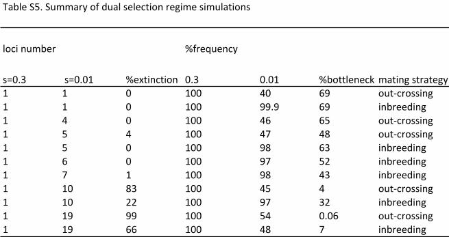
!"#$%&'()&'*++",-&./&0*"$&1%$%234.5&,%64+%&14+*$"34.51

$.24&5*+#%, 7/,%8*%52-

19:); &19:):< 7%=345234.5 :); :):< 7#.33$%5%2> +"3456&13,"3%6-< < : <:: ?: @A .*3B2,.11456< < : <:: AA)A @A 45#,%%0456< ? : <:: ?@ @( .*3B2,.11456< ( ? <:: ?C ?D .*3B2,.11456< ( : <:: AD @; 45#,%%0456< @ : <:: AC (E 45#,%%0456< C < <:: AD ?; 45#,%%0456< <: D; <:: ?( ? .*3B2,.11456< <: EE <:: AC ;E 45#,%%0456< <A AA <:: (? :):@ .*3B2,.11456< <A @@ <:: ?D C 45#,%%0456

Supplementary Information Population selection cost program methodology The program used to simulate selection cost was written in perl by RG Allaby, available to download from the Allaby group website: (http://www2.warwick.ac.uk/fac/sci/lifesci/research/archaeobotany/downloads/). Initialization The program consists of the core algorithm (population_selector.pl), and a wrap that determines the number of times the core algorithm is executed, and extracts summary statistics (selector.pl). The input parameters are contained in a text file (parameters). A second text file (selection_coefficients) lists the selection coefficients and values of lambda for each locus, if there are variable values between loci. The parameters the program takes are as follows (grey indicates parameter values not used in this study, but require an initializing value of 0 input): 1. population size 2. number of genes under selection 3. selection coefficient (if there is just one) 4. maximum fecundity (see main manuscript for an explanation of this) 5. number of generations to simulate 6. number of sexes - 1 is hemaphrodite, 2 is males and females 7. unused variable 8. dominance options (a) 1 all have same lambda, 2 randomly assign lambda to different mutants 9. dominance options (b)lambda (if all the same) determines dominance, 0 fully recessive, 1 fully dominant. 10. unused variable 11. mutation rate 12. variable selection coefficient option: 0 all have same s value determined by option 3, 1 look up selection coefficients and associated lambda values in selection_coefficients file. 13. mating strategy, 0-1, the proportion of matings that are self-fertilization events. 14. gene flow, 0-1 immigrant rate as defined by a proportion of the carrying capacity of individuals arriving from a non-selective environment each generation The core algorithm (population_selection.pl) The simulation begins with an initialization of the population in which individuals are assigned wild type alleles for all loci under selection. A log of wild type frequency and mutant frequency is written to an output file (outfile) for each generation, as well as the population size for that generation. An advantageous mutation occurred with a probability equal to the mutation rate, and was attributed to an individual in the population. The next generation of individuals was then generated by randomly selecting an individual from the previous generation, from which a gamete would be generated by randomly selecting one or other of the alleles of that individual for each locus. Therefore all loci are modeled as unlinked in this simulation. A second gamete was then generated with a probability equal to the mating strategy variable of

selecting the same parent source. Once an individual had been generated, it was challenged such that its probability of survival was given as (su):    

       

!

su = " i1

k

#         (1)  

 For k loci, where  ωI is the fitness of the ith locus as given by:  

!

" i =1# si         (2)    Where si is the selection coefficient of the ith locus. The selection coefficient of the ith locus was moderated by the value lambda for heterozygotes (Shet) such that

!

sihet = "si (3) A value of 0 was taken for lambda in all simulations in this study to represent recessive mutations, which represent the majority of known mutations associated with domestication. In the first generation this step was repeated for a number of times equal to the population size, and inevitably led to a number of individuals in the next generation which were fewer than this value. In subsequent generations the number of attempts at making new individuals was given by

!

Nattempts = Nn"1mf (4) For (Nattempts < initial population size), where Nattempts is the number of individuals created then challenged, Nn-1 is the number of individuals in the previous generation and mf is the maximum fecundity parameter. Where this condition was violated, the initial population size was used, representing the carrying capacity of the environment. This process was iterated for the specified number of generations. The wrap algorithm (selector.pl) The second program calls the first core algorithm for a defined number of trials and in each trial records the out put file (outfile), and calculates the mean and variance each generation of the population size, and the mutant allele frequency for each locus. The mean of the means are then calculated for all loci for each generation, as well as the number of trials in which populations went extinct each generation and the cumulative proportion of trials in which extinction had occurred. These values are collated into a second out put file (otheroutfile). Standing variation A variant of the population_selector.pl program was used to study standing variation called population_selector_SV.pl. This required some changes in data structure in initialize populations to account for standing variation which were set (hard coded) to start at frequencies of 50% in genotype proportions that accurately reflected the mating strategy.