Applied Mathematics Letters 24 (2011) 1124–1129

Contents lists available at ScienceDirect

Applied Mathematics Letters

journal homepage: www.elsevier.com/locate/aml

The limits of Riemann solutions to the isentropic magnetogasdynamics✩

Chun Shen ∗

School of Mathematics and Information, Ludong University, Yantai, Shandong Province, 264025, PR China

a r t i c l e i n f o

Article history:Received 20 May 2010Received in revised form 7 October 2010Accepted 18 October 2010

Keywords:Isentropic magnetogasdynamicsTransport equationsRiemann problemDelta shock wave

a b s t r a c t

The objective of this note is to prove that the Riemann solutions of the isentropicmagnetogasdynamics equations converge to the corresponding Riemann solutions of thetransport equations by letting both the pressure and the magnetic field vanish. The deltashock wave can be obtained as the limit of two shock waves and the vacuum state can beobtained as the limit of two rarefaction waves. Moreover the relation between the speedof formation of singular density and those of the vanishing pressure and the vanishingmagnetic field is discussed in detail.

© 2011 Elsevier Ltd. All rights reserved.

1. Introduction

In this note, we consider the conservation law system which governs the one-dimensional unsteady simple flow of anisentropic, inviscid and perfectly conducting compressible fluid subject to a transverse magnetic field as [1]:

ρt + (ρu)x = 0,(ρu)t + (p + ρu2

+ B2/2µ)x = 0. (1)

In which ρ ≥ 0, u, p ≥ 0, B ≥ 0 andµ > 0 represent the density, velocity, pressure, transverse magnetic field andmagneticpermeability, respectively. Moreover, p and B are defined as p = k1ργ and B = k2ρ where k1 and k2 are positive constantsand γ is the adiabatic constant in the range 1 ≤ γ ≤ 2 for most gases.

The Riemann problem and interactions of elementary waves for (1) are well investigated in [1]. Here we want to knowwhether the limits of Riemann solutions to (1) converge to the corresponding Riemann solutions to the formal limit system

ρt + (ρu)x = 0,(ρu)t + (ρu2)x = 0, (2)

by letting the pressure and themagnetic field disappear, namely letting k1 → 0 and k2 → 0 in (1). The system (2) is nothingbut the transport equations (also called the pressureless Euler equations)whose Riemann problemhas beenwell establishedin [2] and the delta shock wave occurs in the Riemann solutions; also see [3–6] for the related results. About the delta shockwave, we can see the recent survey [7] and the references therein.

In fact, the similar problems on the Euler equations have been carried out for the isentropic case [8] and the isothermalcase [9,10] by letting the pressure term vanish. We can also refer to [11–15] for the related work. In the present note wegeneralize the above results to (1), namely we analyze the formation of the delta shockwave as the limit of two shockwavesand the vacuum state as the limit of two rarefaction waves in the Riemann solutions to (1) as k1, k2 → 0. It is interesting to

✩ This work is supported by the National Natural Science Foundation of China (11001116, 10901077) and the Shandong Provincial Natural ScienceFoundation (ZR2010AL012).∗ Tel.: +86 535 6697510; fax: +86 535 6681264.

E-mail address: shenchun3641@sina.com.

0893-9659/$ – see front matter© 2011 Elsevier Ltd. All rights reserved.doi:10.1016/j.aml.2011.01.038

C. Shen / Applied Mathematics Letters 24 (2011) 1124–1129 1125

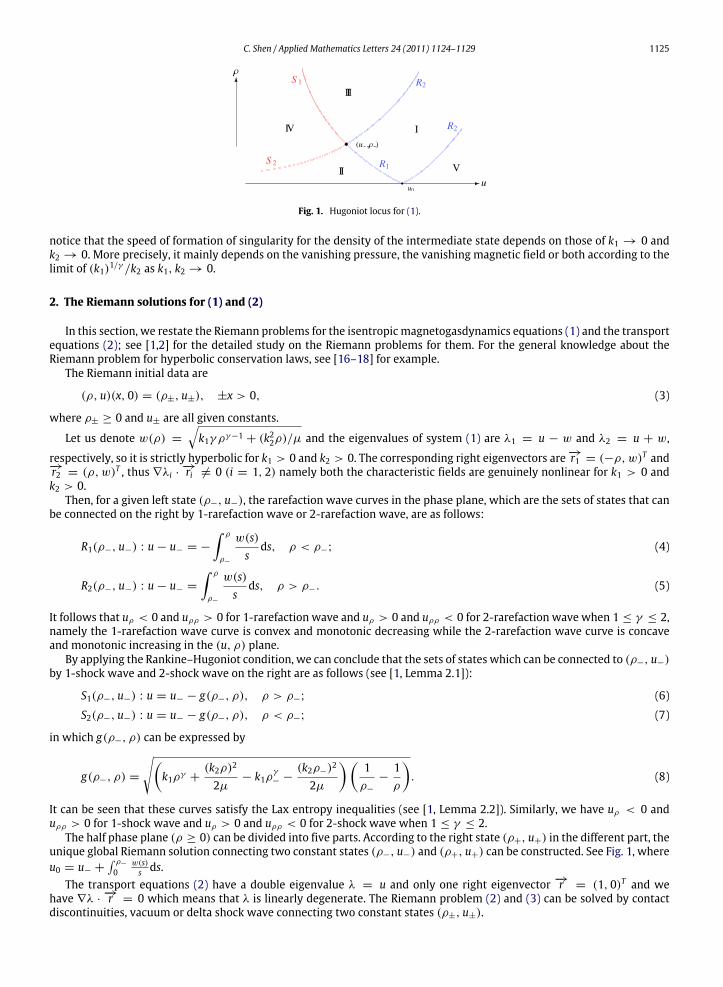
Fig. 1. Hugoniot locus for (1).

notice that the speed of formation of singularity for the density of the intermediate state depends on those of k1 → 0 andk2 → 0. More precisely, it mainly depends on the vanishing pressure, the vanishing magnetic field or both according to thelimit of (k1)1/γ /k2 as k1, k2 → 0.

2. The Riemann solutions for (1) and (2)

In this section, we restate the Riemann problems for the isentropic magnetogasdynamics equations (1) and the transportequations (2); see [1,2] for the detailed study on the Riemann problems for them. For the general knowledge about theRiemann problem for hyperbolic conservation laws, see [16–18] for example.

The Riemann initial data are

(ρ, u)(x, 0) = (ρ±, u±), ±x > 0, (3)

where ρ± ≥ 0 and u± are all given constants.

Let us denote w(ρ) =

k1γ ργ−1 + (k22ρ)/µ and the eigenvalues of system (1) are λ1 = u − w and λ2 = u + w,

respectively, so it is strictly hyperbolic for k1 > 0 and k2 > 0. The corresponding right eigenvectors are −→r1 = (−ρ,w)T and−→r2 = (ρ,w)T , thus ∇λi ·

−→ri = 0 (i = 1, 2) namely both the characteristic fields are genuinely nonlinear for k1 > 0 andk2 > 0.

Then, for a given left state (ρ−, u−), the rarefaction wave curves in the phase plane, which are the sets of states that canbe connected on the right by 1-rarefaction wave or 2-rarefaction wave, are as follows:

R1(ρ−, u−) : u − u− = −

∫ ρ

ρ−

w(s)s

ds, ρ < ρ−; (4)

R2(ρ−, u−) : u − u− =

∫ ρ

ρ−

w(s)s

ds, ρ > ρ−. (5)

It follows that uρ < 0 and uρρ > 0 for 1-rarefaction wave and uρ > 0 and uρρ < 0 for 2-rarefaction wave when 1 ≤ γ ≤ 2,namely the 1-rarefaction wave curve is convex and monotonic decreasing while the 2-rarefaction wave curve is concaveand monotonic increasing in the (u, ρ) plane.

By applying the Rankine–Hugoniot condition, we can conclude that the sets of states which can be connected to (ρ−, u−)by 1-shock wave and 2-shock wave on the right are as follows (see [1, Lemma 2.1]):

S1(ρ−, u−) : u = u− − g(ρ−, ρ), ρ > ρ−; (6)

S2(ρ−, u−) : u = u− − g(ρ−, ρ), ρ < ρ−; (7)

in which g(ρ−, ρ) can be expressed by

g(ρ−, ρ) =

k1ργ +

(k2ρ)2

2µ− k1ρ

γ− −

(k2ρ−)2

2µ

1ρ−

−1ρ

. (8)

It can be seen that these curves satisfy the Lax entropy inequalities (see [1, Lemma 2.2]). Similarly, we have uρ < 0 anduρρ > 0 for 1-shock wave and uρ > 0 and uρρ < 0 for 2-shock wave when 1 ≤ γ ≤ 2.

The half phase plane (ρ ≥ 0) can be divided into five parts. According to the right state (ρ+, u+) in the different part, theunique global Riemann solution connecting two constant states (ρ−, u−) and (ρ+, u+) can be constructed. See Fig. 1, whereu0 = u− +

ρ−

0w(s)s ds.

The transport equations (2) have a double eigenvalue λ = u and only one right eigenvector −→r = (1, 0)T and wehave ∇λ ·

−→r = 0 which means that λ is linearly degenerate. The Riemann problem (2) and (3) can be solved by contactdiscontinuities, vacuum or delta shock wave connecting two constant states (ρ±, u±).

1126 C. Shen / Applied Mathematics Letters 24 (2011) 1124–1129

For the case u− < u+, there is no characteristic passing through the region u− < ξ = x/t < u+ and vacuum appears.The solution can be expressed as

(ρ, u)(x, t) =

(ρ−, u−), −∞ < ξ ≤ u−,(0, ξ), u− ≤ ξ ≤ u+,(ρ+, u+), u+ ≤ ξ < ∞.

(9)

For the case u− = u+, it is easy to see that the constant states (ρ±, u±) can be connected by a contact discontinuity.For the case u− > u+, a solution containing aweighted δ-measure supported on a line should be constructed. Let x = x(t)

be a discontinuity curve, we consider the measure solution in the form

(ρ, u)(x, t) =

(ρ−, u−), x < x(t),(β(t)δ(x − x(t)), uδ(t)), x = x(t),(ρ+, u+), x > x(t).

(10)

In order to define the measure solutions as above, like as in [2,8,14], the two-dimensional weighted δ-measure p(s)δSsupported on a smooth curve S = {(x(s), t(s)) : a < s < b} should be introduced as follows:

⟨p(s)δS, ψ(x(s), t(s))⟩ =

∫ b

ap(s)ψ(x(s), t(s))ds, (11)

for any ψ ∈ C∞

0 (R × R+).The measure solution (10) satisfies the generalized Rankine–Hugoniot condition

dxdt

= uδ(t),dβ(t)dt

= [ρ]uδ(t)− [ρu],d(β(t)uδ(t))

dt= [ρu]uδ(t)− [ρu2

], (12)

where [ρ] = ρ(x(t)+ 0, t)− ρ(x(t)− 0, t) denotes the jump of ρ across the discontinuity x = x(t), etc.Let us denote σ =

√ρ−u−+

√ρ+u+

√ρ−+

√ρ+

. Through solving (12), we obtain

x(t) = σ t, uδ(t) = σ , β(t) =√ρ−ρ+(u− − u+)t. (13)

The unique entropy solution (10) with (13) can be chosen from (12) obeying the δ-entropy condition: u+ < σ < u−.

3. The limits of Riemann solutions of (1) as k1, k2 → 0

This section is devoted to proving that the limits of the Riemann solutions of (1) are exactly those of (2) as k1, k2 → 0.The proof is based on the detailed analysis of the Riemann problem of (1) and (3). Indeed, this analysis permits us to exhibitthe limits of the solutions to the Riemann problem of (1) and (3) as k1, k2 → 0, which are nothing but the expected solutionsto the Riemann problem of (2) and (3).

At first, we study the formation of delta shock wave in the Riemann problem (1) and (3) when u− > u+ as k1, k2 → 0.The curves S1 and S2 in the phase plane (see Fig. 1) become steeper as k1, k2 → 0, thus it follows that (ρ+, u+) ∈ IV (ρ−, u−)for sufficiently small k1, k2 if u− > u+.

If (ρ+, u+) ∈ IV (ρ−, u−), then the Riemann solution consists of two shockwaves S1, S2 and an intermediate state (ρ∗, u∗)besides two constant states (ρ±, u±). It can be derived from (6) and (7) that (ρ∗, u∗) is determined by

u∗ = u− − g(ρ−, ρ∗), ρ∗ > ρ−; (14)

u+ = u∗ − g(ρ∗, ρ+), ρ+ < ρ∗. (15)

The addition of (14) and (15) gives

g(ρ−, ρ∗)+ g(ρ∗, ρ+) = u− − u+. (16)

For given ρ± > 0, letting k1, k2 → 0 in (16), we have

limk1,k2→0

k1ρ

γ∗ +

(k2ρ∗)2

2µ·

1ρ−

−1ρ∗

+

1ρ+

−1ρ∗

= u− − u+. (17)

Noticing that ρ∗ > ρ±, one can see that 1ρ−

−1ρ+

<

1ρ−

−1ρ∗

+

1ρ+

−1ρ∗

<

1ρ−

+

1ρ+

. (18)

Thus we have limk1,k2→0

k1ρ

γ∗ + (k2ρ∗)2/(2µ) > 0, which implies that limk1,k2→0 ρ∗ = ∞.

C. Shen / Applied Mathematics Letters 24 (2011) 1124–1129 1127

It can be derived from (17) that

limk1,k2→0

k1ρ

γ∗ +

(k2ρ∗)2

2µ=

√ρ−ρ+(u− − u+)√ρ− +

√ρ+

. (19)

From (19), we can see that the growth rate of ρ∗ → ∞ depends on those of k1 → 0 and k2 → 0. Moreover, we can alsoregard ρ∗ as the function of k1 and k2 and denote it with ρ∗ = ρ∗(k1, k2). Let us rewrite (19) in the following form

limk1,k2→0

k1ργ∗ + limk1,k2→0

(k2ρ∗)2

2µ= M, (20)

where M =ρ−ρ+(u−−u+)

2

(√ρ−+

√ρ+)2

.Taking into account k1, k2, µ > 0, we can see that

0 ≤ limk1,k2→0

k1ργ∗ , limk1,k2→0

(k2ρ∗)2

2µ≤ M. (21)

Furthermore, we have

0 ≤ limk1,k2→0

(k1)1/γ ρ∗ ≤ M1/γ , 0 ≤ limk1,k2→0

k2ρ∗ ≤2µM. (22)

Now our discussion can be divided into the following three cases according to the relation between the speed of k1 → 0and that of k2 → 0.(i) If limk1,k2→0(k1)1/γ /k2 = 0, then we have

limk1,k2→0

k1ργ∗ = 0, limk1,k2→0

(k2ρ∗)2

2µ= M. (23)

In this case the growth rate of ρ∗ → ∞ mainly depends on that of k2 → 0, namely the developing speed of the singularityof ρ∗ is mainly determined by the speed of vanishing magnetic field. More precisely, we have ρ∗ ∼ 1/k2 as k1, k2 → 0.(ii) If limk1,k2→0(k1)1/γ /k2 = ∞, then we have

limk1,k2→0

k1ργ∗ = M, limk1,k2→0

(k2ρ∗)2

2µ= 0. (24)

Like as before, the growth rate of ρ∗ → ∞ mainly depends on that of k1 → 0. Now the developing speed of the singularityof ρ∗ is mainly determined by the speed of vanishing pressure, namely ρ∗ ∼ (k1)−1/γ as k1, k2 → 0.(iii) If limk1,k2→0(k1)1/γ /k2 = c , let us denote x = limk1,k2→0 k2ρ∗, then it follows from (20) that

2µcγ xγ + x2 = 2µM. (25)

It can be shown that

limk1,k2→0

k1ργ∗ = cγ xγ , limk1,k2→0

(k2ρ∗)2

2µ=

x2

2µ. (26)

In this case, the growth rate of ρ∗ → ∞ depends on both of those of k1 → 0 and k2 → 0. It is clear that the developingspeed of the singularity of ρ∗ is determined by both the speed of vanishing pressure and that of vanishing magnetic fieldfrom the relation ρ∗ ∼ (k1)−1/γ

∼ 1/k2 as k1, k2 → 0.

Remark 1. For the special situations γ = 1 and γ = 2, x can be explicitly expressed as x =2µM + µ2c2 −µc for γ = 1

and x =2µM/(2µc2 + 1) for γ = 2, respectively.

From the above analysis, we can see that the density of the intermediate state ρ∗ becomes singular when both thepressure and magnetic field vanish. Now we discuss the velocity of the intermediate state u∗ in the limit and it followsfrom (14) and (19) that

limk1,k2→0

u∗ = u− −

√ρ+(u− − u+)

√ρ− +

√ρ+

=

√ρ−u− +

√ρ+u+

√ρ− +

√ρ+

= σ = uδ(t). (27)

The Rankine–Hugoniot conditions for both shocks S1 and S2 are

σ1(ρ∗ − ρ−) = ρ∗u∗ − ρ−u−, σ2(ρ+ − ρ∗) = ρ+u+ − ρ∗u∗. (28)

1128 C. Shen / Applied Mathematics Letters 24 (2011) 1124–1129

Thus the limits of the propagation speeds of the 1-shock wave and 2-shock wave can be calculated respectively by

limk1,k2→0

σ1 = limk1,k2→0

ρ∗u∗ − ρ−u−

ρ∗ − ρ−

= σ , (29)

limk1,k2→0

σ2 = limk1,k2→0

ρ+u+ − ρ∗u∗

ρ+ − ρ∗

= σ . (30)

From the above results, it can be found that the two shocks coincide as k1, k2 → 0 whose velocities are identical with thatof the delta shock of the transport equations (2) with the same Riemann initial data (ρ±, u±).

It is easily derived from (28) that

(σ1 − σ2)ρ∗ = ρ+u+ − ρ−u− + σ1ρ− − σ2ρ+. (31)

With (29) and (30) in mind, taking the limit in (31) leads to

limk1,k2→0

(σ1 − σ2)ρ∗ = [ρu] − σ [ρ]. (32)

Hence, we have

limk1,k2→0

∫ σ2t

σ1tρ∗dx = (σ [ρ] − [ρu])t =

√ρ−ρ+(u− − u+)t = β(t), (33)

which is exactly the strength of the delta shock wave of the transport equations (2) with the same Riemann initial data(ρ±, u±).

Remark 2. From above, we can see that ρ∗ has the same singularity as a weighted Dirac delta function at x = σ t in the limitsituation, which is called the delta shock wave in [19]. From (27), (29), (30) and (33), we can also see that the limit of theRiemann solution of (1) and (3) as k1, k2 → 0 is (10) with (13) when u− > u+, which is exactly the corresponding Riemannsolution of (2) and (3) and obviously obeys the generalized Rankine–Hugoniot condition (12). For the strict proof about theweak limit of the Riemann solution of (1) and (3) as k1, k2 → 0 is that of (2) and (3), the process is similar to Theorem 3.1in [8] and Theorem 6.3 in [14] and we omit it here.

Second, we study the formation of contact discontinuity in the Riemann problem (1) and (3) for the special case u− = u+

as k1, k2 → 0. For u− = u+, (ρ±, u±) can be connected by S1, an intermediate state (ρ∗, u∗) and R2 for ρ+ > ρ− or by R1,(ρ∗, u∗) and S2 for ρ+ < ρ−. In particular, (ρ, u) is a constant state (ρ−, u−) for ρ− = ρ+.

If ρ+ > ρ−, (ρ∗, u∗) between S1 and R2 can be obtained from (14) and

u+ − u∗ =

∫ ρ+

ρ∗

w(s)s

ds, ρ+ > ρ∗. (34)

Noticing that ρ∗ is bounded here and letting k1, k2 → 0 in (34), it can be immediately obtained that limk1,k2→0 u∗ = u+.Noting u+ = u− and combining (14) and (34), we have

g(ρ−, ρ∗)−

∫ ρ+

ρ∗

w(s)s

ds = 0. (35)

Furthermore, we haveργ∗ +

(k2ρ∗)2

2µk1− ρ

γ− −

(k2ρ−)2

2µk1

1ρ−

−1ρ∗

−

∫ ρ+

ρ∗

γ sγ−1 + (k22s)/(µk1)

sds = 0, (36)

which implies that limk1,k2→0 ρ∗ = ρ−.Thus, we get

limk1,k2→0

σ1 = limk1,k2→0

ρ∗u∗ − ρ−u−

ρ∗ − ρ−

= limk1,k2→0

u∗ +

ρ−(u∗ − u−)

ρ∗ − ρ−

= u−. (37)

On the other hand, we have

limk1,k2→0

λ2(ρ∗, u∗) = limk1,k2→0

u∗ +

k1γ ρ

γ−1∗ + (k22ρ∗)/µ

= u−, (38)

limk1,k2→0

λ2(ρ+, u+) = limk1,k2→0

u+ +

k1γ ρ

γ−1+ + (k22ρ+)/µ

= u+ = u−. (39)

C. Shen / Applied Mathematics Letters 24 (2011) 1124–1129 1129

According to (37)–(39), we can see that both S1 and R2 degenerate to the contact discontinuity J as k1, k2 → 0. The similaranalysis can be carried out for ρ+ < ρ− and both R1 and S2 degenerate to J in the limit situation.

Finally, we consider the formation of vacuum state in the Riemann problem (1) and (3) when u− < u+ as k1, k2 → 0. Thecurves R1 and R2 in the phase plane (see Fig. 1) also become steeper as k1, k2 → 0, and it follows that (ρ+, u+) ∈ V (ρ−, u−)for sufficiently small k1, k2 if u− < u+. Hence, the intermediate state (ρ∗, u∗) becomes a vacuum state (ρ∗, u∗) = (0, ξ)with u1 ≤ ξ ≤ u2. From (4) and (5), we can see that the limits of u1 and u2 can be calculated respectively by

limk1,k2→0

u1 = u− − limk1,k2→0

∫ 0

ρ−

k1γ sγ−1 + (k22s)/µ

sds = u−, (40)

limk1,k2→0

u2 = u+ − limk1,k2→0

∫ ρ+

0

k1γ sγ−1 + (k22s)/µ

sds = u+. (41)

Thus the limit of Riemann solution to (1) is exactly (9) in this case. Based on the above analysis, when k1, k2 → 0, wecan see that the left boundary of 1-rarefaction wave and the right boundary of 2-rarefaction wave become two contactdiscontinuities of the transport equations (2) with the same Riemann initial data (ρ±, u±) and the vacuum state fills up theregion between the two contact discontinuities.

In brief, we summarize our results in the following.

Theorem 1. For any given Riemann initial data (u±, v±), the limits of the Riemann solutions of the isentropicmagnetogasdynamics equations (1) are exactly the Riemann solutions of the transport equations (2) with the same Riemanninitial data as k1, k2 → 0.

Acknowledgements

The author is grateful to the anonymous referee for the valuable comments which improve the presentation of the papergreatly.

References

[1] T. Raja Sekhar, V.D. Sharma, Riemann problem and elementary wave interactions in isentropic magnetgasdynamics, Nonlinear Anal. RWA 11 (2010)619–636.

[2] W. Sheng, T. Zhang, The Riemann problem for the transportation equations in gas dynamics, Mem. Amer. Math. Soc. 137 (N654) (1999) AMS:Providence.

[3] F. Bouchut, On zero pressure gas dynamics, in: Advances in Kinetic Theory and Computing, in: Ser. Adv. Math. Appl. Sci., vol. 22, World Sci. Publishing,River Edge, NJ, 1994, pp. 171–190.

[4] Y. Brenier, E. Grenier, Sticky particles and scalar conservation laws, SIAM J. Numer. Anal. 35 (1998) 2317–2338.[5] W.E., Yu.G. Rykov, Ya.G. Sinai, Generalized variational principles, global weak solutions and behavior with random initial data for systems of

conservation laws arising in adhesion particle dynamics, Commun. Math. Phys. 177 (1996) 349–380.[6] F. Huang, Z. Wang, Well-posedness for pressureless flow, Commun. Math. Phys. 222 (2001) 117–146.[7] V.M. Shelkovich, δ- and δ′-shock wave types of singular solutions of systems of conservation laws and transport and concentration processes, Russian

Math. Surveys 63 (2008) 473–546.[8] G.Q. Chen, H. Liu, Formation of δ-shocks and vacuum states in the vanishing pressure limit of solutions to the Euler equations for isentropic fluids,

SIAM J. Math. Anal. 34 (2003) 925–938.[9] J. Li, Note on the compressible Euler equations with zero temperature, Appl. Math. Lett. 14 (2001) 519–523.

[10] R.J. Leveque, The dynamics of pressureless dust clouds and delta waves, J. Hyperbolic Differ. Equ. 1 (2004) 315–327.[11] G.Q. Chen, H. Liu, Concentration and cavition in the vanishing pressure limit of solutions to the Euler equations for nonisentropic fluids, Physica D 189

(2004) 141–165.[12] D. Mitrovic, M. Nedeljkov, Delta-shock waves as a limit of shock waves, J. Hyperbolic Differ. Equ. 4 (2007) 629–653.[13] C. Shen, M. Sun, Z. Wang, Limit relations for three simple hyperbolic systems of conservation laws, Math. Meth. Appl. Sci. 33 (2010) 1317–1330.[14] C. Shen, M. Sun, Formation of delta shocks and vacuum states in the vanishing pressure limit of Riemann solutions to the perturbed Aw–Rascle model,

J. Differ. Equ. 249 (2010) 3024–3051.[15] G. Yin, W. Sheng, Delta shocks and vacuum states in vanishing pressure limits of solutions to the relativistic Euler equations for polytropic gases, J.

Math. Anal. Appl. 355 (2009) 594–605.[16] T. Chang, L. Hsiao, The Riemann Problem and Interaction of Waves in Gas Dynamics, in: Pitman Monographs and Surveys in Pure and Applied

Mathematics, vol. 41, Longman Scientific and Technical, 1989.[17] D. Serre, Systems of Conservation Laws 1/2, Cambridge Univ. Press, Cambridge, 1999/2000.[18] J. Smoller, Shock Waves and Reaction–Diffusion Equations, Springer-Verlag, NewYork, 1994.[19] D. Tan, T. Zhang, Y. Zheng, Delta-shock waves as limits of vanishing viscosity for hyperbolic systems of conservation laws, J. Differ. Equ. 112 (1994)

1–32.