The lightest Higgs boson mass in the Minimal ... · The lightest Higgs boson mass in the Minimal Supersymmetric Standard Model∗ J.A. Casas1, 2, J. R. Espinosa †, M. Quir´os2

arX

iv:h

ep-p

h/94

0738

9v1

27

Jul 1

994

The lightest Higgs boson mass in theMinimal Supersymmetric Standard Model∗

J.A. Casas1,2, J. R. Espinosa2†, M. Quiros2 and A. Riotto2‡

1CERN, TH Division, CH-1211 Geneva 23, Switzerland

2Instituto de Estructura de la Materia, CSIC

Serrano 123, 28006-Madrid, Spain

Abstract

We compute the upper bound on the mass of the lightest Higgs boson in the

Minimal Supersymmetric Standard Model in a model-independent way, includ-

ing leading (one-loop) and next-to-leading order (two-loop) radiative corrections.

We find that (contrary to some recent claims) the two-loop corrections are nega-

tive with respect to the one-loop result and relatively small (<∼ 3%). After defining

physical (pole) top quark mass Mt, by including QCD self-energies, and physical

Higgs mass MH , by including the electroweak self-energies Π(

M2H

)

− Π(0), we

obtain the upper limit on MH as a function of supersymmetric parameters. We

include as supersymmetric parameters the scale of supersymmetry breaking MS ,

the value of tan β and the mixing between stops Xt = At + µ cot β (which is re-

sponsible for the threshold correction on the Higgs quartic coupling). Our results

do not depend on further details of the supersymmetric model. In particular, for

MS ≤ 1 TeV, maximal threshold effect X2t = 6M2

S and any value of tan β, we

find MH ≤ 140 GeV for Mt ≤ 190 GeV. In the particular scenario where the top

is in its infrared fixed point we find MH ≤ 86 GeV for Mt = 170 GeV.

CERN–TH.7334/94July 1994

CERN–TH.7334/94IEM–FT–87/94hep-ph/9407389

∗Work partly supported by CICYT under contract AEN94-0928, and by the European Union undercontract No. CHRX-CT92-0004.

†Supported by a grant of Comunidad de Madrid, Spain.‡On leave of absence from International School of Advanced Studies, ISAS, Trieste.

http://arXiv.org/abs/hep-ph/9407389v1

http://arXiv.org/abs/hep-ph/9407389

1 Introduction

There are good reasons to believe that the Standard Model (SM) is not the ultimatetheory since it is unable to answer many fundamental questions. One of them, whyand how the electroweak and the Planck scales are so hierarchically separated, has mo-tivated the proposal of the Minimal Supersymmetric extension of the Standard Model(MSSM) as the underlying theory at scales of order 1 TeV. Indeed, the supersymmet-ric scale cannot be very large not to spoil the solution to the hierarchy problem, butthe ambiguity about its maximal allowable size makes it very difficult to give model–independent predictions testable in accelerators.

Fortunately, the supersymmetric predictions for the upper bound on the lightestHiggs boson mass represent a (perhaps unique) exception to this rule. Therefore, theyare crucial for the experimental verification of supersymmetry. This importance isreinforced by the fact that uncovering the Higgs boson of the SM is one of the mainchallenges for present (LEP, Tevatron) and future (LEP-200, LHC) accelerators. Muchwork has been recently devoted to this subject [1–10], but still there is a substantialdisagreement on the final results (see e.g. [5,9,10]), especially concerning the two–loopcorrections (which, as we will see, are crucial).

The aim of this paper is to evaluate the two-loop predictions of the MSSM on thelightest Higgs mass in a consistent and model-independent way. In fact, our resultswill not depend on the details of the MSSM (e.g. the assumption or not of universalityof the soft breaking terms, gauge and Yukawa unification, etc.). Actually, when we willrefer to the MSSM, we will simply mean the supersymmetric version of the SM withminimal particle content. The consistency of the approach will allow us to show up thereasons of the disagreement between previous results. We also give the predictions onthe Higgs mass for a particularly appealing scenario, namely the assumption that therecently detected top quark [11] has the Yukawa coupling in its infrared fixed point. Itwill turn out that in this case the Higgs boson should be just around the corner.

Let us briefly review the status of the subject and the most recent contributions onit. The MSSM has an extended Higgs sector with two Higgs doublets with oppositehypercharges: H1, responsible for the mass of the charged leptons and the down-typequarks, and H2, which gives a mass to the up-type quarks. After the Higgs mechanismthere remain three physical scalars, two CP-even and one CP-odd Higgs bosons. Inparticular, the lightest CP-even Higgs boson mass satisfies the tree-level bound

m2H ≤ M2

Z cos2 2β, (1.1)

where tan β = v2/v1 is the ratio of the Vacuum Expectation Values (VEV’s) of theneutral components of the two Higgs fields H2 and H1, respectively. The relation(1.1) implies that m2

H < M2Z , for any value of tan β which, in turn, implies that

it should be found at LEP-200 [1]. However, the tree level relation (1.1) is spoiledby one-loop radiative corrections, which were computed by several groups using: theeffective potential approach [2], diagrammatic methods [3] and renormalization group

1

(RG) techniques [4]. All methods found excellent agreement with each other and largeradiative corrections, mainly controlled by the top Yukawa coupling, which could makethe lightest CP-even Higgs boson to escape experimental detection at LEP-200. Inparticular, the RG approach (which will be followed in the present paper) is based onthe fact that supersymmetry decouples and below the scale of supersymmetry breakingMS the effective theory is the SM. Assuming M2

Z ≪ M2S the tree-level bound (1.1) is

saturated at the scale MS and the effective SM at scales between MZ and MS containsthe Higgs doublet

H = H1 cos β + iσ2H∗2 sin β, (1.2)

with a quartic coupling taking, at the scale MS, the (tree level) value

λ =1

4(g2 + g′2) cos2 2β. (1.3)

In these analyses [4] the Higgs mass was considered at the tree-level, improved by one-loop renormalization group equations (RGE) in the γ– and β–functions, thus collectingall leading logarithm corrections.

Since the relative size of one-loop corrections to the Higgs mass is large (mainly forlarge top quark mass and/or small tree level Higgs mass) it was compelling to analyzethem at the two-loop level. A first step in that direction was given in ref. [5] wheretwo-loop RGE improved tree level Higgs masses were considered. It was found thattwo-loop corrections were negative and small. In ref. [5] the Higgs mass received allleading logarithm and part of the next-to-leading logarithm corrections. Subsequentstudies of the effective potential improved by the RGE [6, 7, 8] have shown that theL-loop improved effective potential with (L+1)-loop RGE is exact up to Lth-to-leadinglogarithm order [7]1. This means that for fully taking into account all next-to-leadinglogarithm corrections the one-loop effective potential (improved by two-loop RGE) isneeded.

Finally, two papers [9, 10] have recently appeared aiming to refine the two-loopanalysis of ref. [5]. The authors of ref. [9], following the RG approach, find that thetwo-loop correction to the Higgs mass is positive and sizeable, whereas the authorsof ref. [10], following diagrammatic [3] and effective potential [2] approaches in theframework of the MSSM with various approximations, find that the two-loop correctionto the Higgs mass is negative and sizeable in contradiction with ref. [9]. As we will seein detail in section 5 we are in disagreement with the results of ref. [9] (showing how acorrect treatment of all the relevant effects would make the results presented in ref. [9]to agree with ours), and in agreement with the overall result of ref. [10] (though notwith the relative size of the two-loop corrections).

In this paper we use the RG approach and the SM one-loop improved effectivepotential with two-loop RGE to compute the lightest Higgs mass of the MSSM up tonext-to-leading logarithm order. At this level of approximation, one has to keep control

1Strictly speaking this has been proven [7] for a theory with a single mass scale.

2

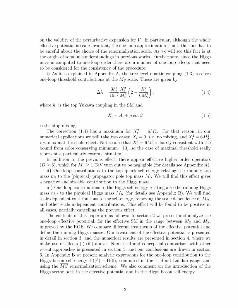
on the validity of the perturbative expansion for V . In particular, although the wholeeffective potential is scale-invariant, the one-loop approximation is not, thus one has tobe careful about the choice of the renormalization scale. As we will see this fact is atthe origin of some misunderstandings in previous works. Furthermore, since the Higgsmass is computed to one-loop order there are a number of one-loop effects that needto be considered for the consistency of the procedure:

i) As it is explained in Appendix A, the tree level quartic coupling (1.3) receivesone-loop threshold contributions at the MS scale. These are given by

∆λ =3h4

t

16π2

X2t

M2S

(

2 − X2t

6M2S

)

, (1.4)

where ht is the top Yukawa coupling in the SM and

Xt = At + µ cotβ (1.5)

is the stop mixing.The correction (1.4) has a maximum for X2

t = 6M2S. For that reason, in our

numerical applications we will take two cases: Xt = 0, i.e. no mixing, and X2t = 6M2

S,i.e. maximal threshold effect. Notice also that X2

t = 6M2S is barely consistent with the

bound from color conserving minimum [13], so the case of maximal threshold reallyrepresent a particularly extreme situation.

In addition to the previous effect, there appear effective higher order operators(D ≥ 6), which for MS ≥ 1 TeV turn out to be negligible (for details see Appendix A).

ii) One-loop contributions to the top quark self-energy relating the running topmass mt to the (physical) propagator pole top mass Mt. We will find this effect givesa negative and sizeable contribution to the Higgs mass

iii) One-loop contributions to the Higgs self-energy relating also the running Higgsmass mH to the physical Higgs mass MH (for details see Appendix B). We will findscale dependent contributions to the self-energy, removing the scale dependence of MH ,and other scale independent contributions. This effect will be found to be positive inall cases, partially cancelling the previous effect.

The contents of this paper are as follows: In section 2 we present and analyze theone-loop effective potential, for the effective SM in the range between MZ and MS,improved by the RGE. We compare different treatments of the effective potential anddefine the running Higgs masses. Our treatment of the effective potential is presentedin detail in section 3, and the numerical results are presented in section 4, where wemake use of effects (i)-(iii) above. Numerical and conceptual comparison with otherrecent approaches is presented in section 5, and our conclusions are drawn in section6. In Appendix B we present analytic expressions for the one-loop contribution to theHiggs boson self-energy Π(q2) − Π(0), computed in the ’t Hooft-Landau gauge andusing the MS renormalization scheme. We also comment on the introduction of theHiggs sector both in the effective potential and in the Higgs boson self-energy.

3

2 The one-loop effective potential

Our starting point in this section will be the effective potential of the Standard Model.This can be written in the ’t Hooft-Landau gauge as [8]

Veff(µ(t), λi(t); φ(t)) ≡ V0 + V1 + · · · , (2.1)

where λi ≡ (g, g′, λ, ht, m2) runs over all dimensionless and dimensionful couplings and

V0, V1 are respectively the tree level potential and the one-loop correction, namely

V0 = −1

2m2(t)φ2(t) +

1

8λ(t)φ4(t), (2.2)

V1 =1

64π2

6m4W (t)

[

logm2

W (t)

µ2(t)− 5

6

]

+ 3m4Z(t)

[

logm2

Z(t)

µ2(t)− 5

6

]

−12m4t (t)

[

logm2

t (t)

µ2(t)− 3

2

]

,

(2.3)

where we have used the MS renormalization scheme [12]. The parameters λ(t) andm(t) are the Standard Model quartic coupling and mass, running with the RGE, whilethe running Higgs field is

φ(t) = ξ(t)φc, (2.4)

φc being the classical field and

ξ(t) = e−∫

t

0γ(t′)dt′ , (2.5)

where γ(t) is the Higgs field anomalous dimension. V1 in eq.(2.3) contains the radiativecorrections where only the top quark and the W, Z gauge bosons are propagating inthe loop. For the moment we will disregard those coming from the Higgs and Goldstoneboson propagation2. They can be easily introduced, as shown in Appendix B, withoutaltering the numerical results that are obtained in this paper. The mass parameters in(2.3) are given by

m2W (t) =

1

4g2(t)φ2(t),

m2Z(t) =

1

4[g2(t) + g′2(t)]φ2(t),

m2t (t) =

1

2h2

t (t)φ2(t),

(2.6)

2In particular, the Goldstone boson contribution to the effective potential generates, on the runningHiggs mass, an infrared logarithmic divergence. This divergence is cancelled when the physical Higgsmass is considered, as will be shown in Appendix B.

4

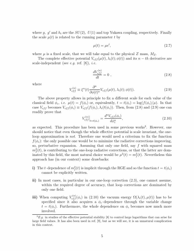
where g, g′ and ht are the SU(2), U(1) and top Yukawa coupling, respectively. Finallythe scale µ(t) is related to the running parameter t by

µ(t) = µet, (2.7)

where µ is a fixed scale, that we will take equal to the physical Z mass, MZ .The complete effective potential Veff(µ(t), λi(t); φ(t)) and its n − th derivative are

scale-independent (see e.g. ref. [8]), i.e.

dV(n)eff

dt= 0 , (2.8)

where

V(n)eff ≡ ξn(t)

∂n

∂φ(t)nVeff(µ(t), λi(t); φ(t)). (2.9)

The above property allows in principle to fix a different scale for each value of theclassical field φc, i.e. µ(t) = f(φc) or, equivalently, t = t(φc) = log(f(φc)/µ). In thatcase Veff becomes Veff(φc) ≡ Veff(f(φc), λi(t(φc)). Then, from (2.8) and (2.9) one canreadily prove that

V(n)eff

∣

∣

∣

t=t(φc)=

dnVeff(φc)

dφnc

, (2.10)

as expected. This procedure has been used in some previous works3. However, oneshould notice that even though the whole effective potential is scale invariant, the one-loop approximation is not. Therefore one would need a criterium to fix the functionf(φc): the only possible one would be to minimize the radiative corrections improving,so, perturbative expansion. Assuming that only one field, say f with squared massm2

f (t), is contributing to the one-loop radiative corrections, or that the latter are dom-inated by this field, the most natural choice would be µ2(t) = m2

f (t). Nevertheless thisapproach has (in our context) some drawbacks:

i) The t–dependence of m2f (t) is implicit through the RGE and so the function t = t(φc)

cannot be explicitly written.

ii) In most cases, in particular in our one-loop correction (2.3), one cannot assume,within the required degree of accuracy, that loop corrections are dominated byonly one field.

iii) When computing V(n)eff (φc) in (2.10) the vacuum energy Ω(λi(t), µ(t)) has to be

specified since it also acquires a φc–dependence through the variable changet = t(φc). Furthermore, the whole dependence on φc becomes now much moreinvolved.

3E.g. in studies of the effective potential stability [8] to control large logarithms that can arise forlarge field values. It has also been used in ref. [9], but as we will see, it is an unnatural complicationin this context.

5

iv) The last, but not the least, drawback is that once one has chosen a particularfunction t(φc), one looses track of scale invariance and so there is no way ofchecking how good the approximation is at the minimum of the effective potential.

For the above mentioned reasons we will keep t and φc as independent variables. Wewill minimize the effective potential (2.1), truncated at one-loop, at some fixed scalet = t∗, i.e.

∂Veff

∂φ(t∗)

∣

∣

∣

∣

∣

φ(t∗)=〈φ(t∗)〉

= 0, (2.11)

which will determine the VEV 〈φ(t∗)〉. Our criterium to fix the scale t∗ will be explainedin the next section. The scale independence of the whole effective potential implies that

d

dt

〈φ(t)〉ξ(t)

= 0. (2.12)

Therefore, assuming that t∗ lies in the region where the one-loop approximation tothe effective potential is reliable, the VEV of the field at any scale can be obtainedthrough4

〈φ(t)〉 = 〈φ(t∗)〉 ξ(t)

ξ(t∗). (2.13)

Accordingly, we must impose

v = 〈φ(tZ)〉 = 〈φ(t∗)〉ξ(tZ)

ξ(t∗), (2.14)

where tZ is defined as µ(tZ) = MZ and

v = (√

2Gµ)−1/2 = 246.22 GeV, (2.15)

is the “measured” VEV for the Higgs field5 [16].We can trade 〈φ(t∗)〉 by m2(t∗) from the condition of minimum (2.11), which trans-

lates, using (2.14), into the boundary condition for m2(t):

m2(t∗)

v2=

1

2λ(t∗)ξ2(t∗) +

3

64π2ξ2(t∗)

1

2g4(t∗)

[

logg2(t∗)ξ2(t∗)v2

4µ2(t∗)− 1

3

]

+1

4[g2(t∗) + g′2(t∗)]

2

[

log[g2(t∗) + g′2(t∗)] ξ2(t∗)v2

4µ2(t∗)− 1

3

]

− 4h4t (t

∗)

[

logh2

t (t∗)ξ2(t∗)v2

2µ2(t∗)− 1

]

.

(2.16)

4Notice that 〈φ(t)〉 defined by (2.13) coincides with the value of φ(t) which minimizes the wholeeffective potential. In the one-loop approximation that we are using this is no longer true, as we willsee later on.

5We are neglecting here one-loop electroweak radiative corrections to the muon β-decay slightlymodifying the relation (2.15), see e.g. ref. [15]. We thank S. Peris for a discussion on this point.

6

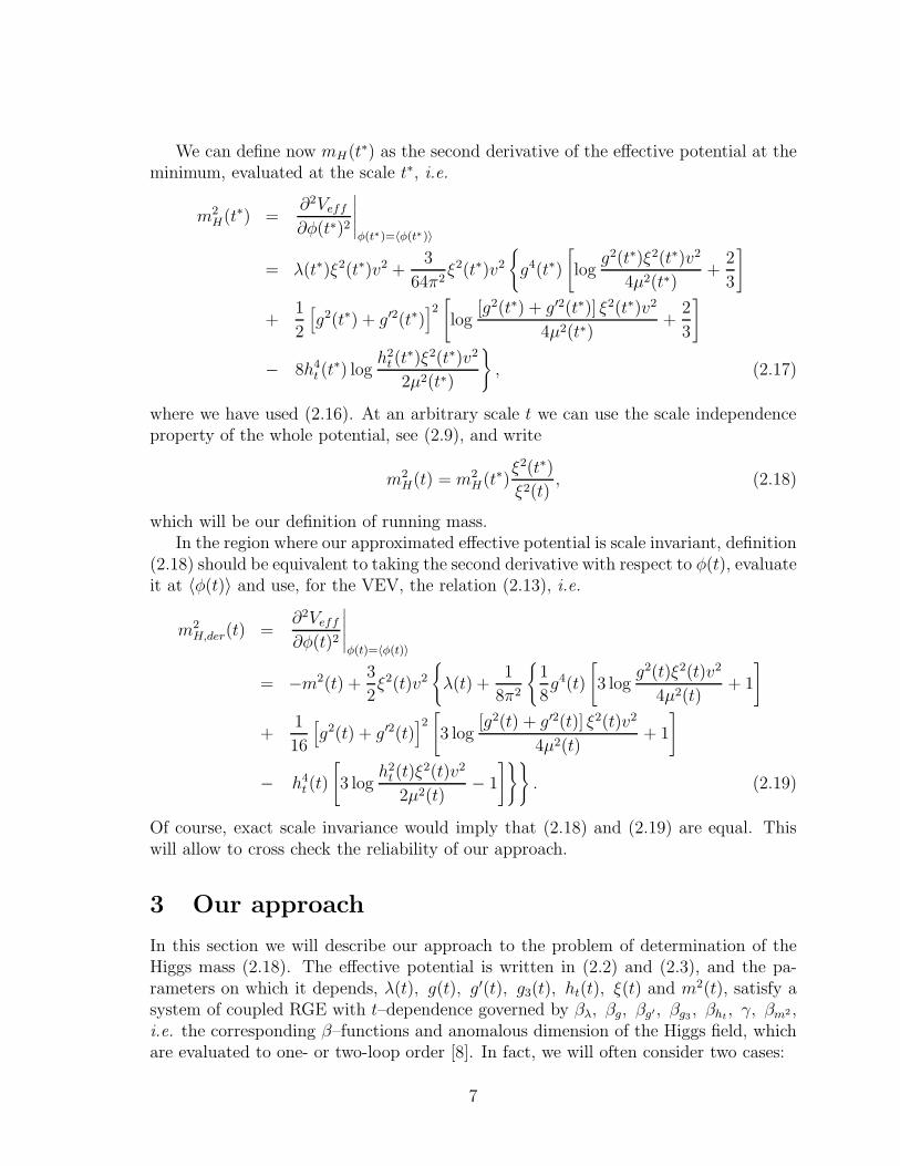
We can define now mH(t∗) as the second derivative of the effective potential at theminimum, evaluated at the scale t∗, i.e.

m2H(t∗) =

∂2Veff

∂φ(t∗)2

∣

∣

∣

∣

∣

φ(t∗)=〈φ(t∗)〉

= λ(t∗)ξ2(t∗)v2 +3

64π2ξ2(t∗)v2

g4(t∗)

[

logg2(t∗)ξ2(t∗)v2

4µ2(t∗)+

2

3

]

+1

2

[

g2(t∗) + g′2(t∗)]2[

log[g2(t∗) + g′2(t∗)] ξ2(t∗)v2

4µ2(t∗)+

2

3

]

− 8h4t (t

∗) logh2

t (t∗)ξ2(t∗)v2

2µ2(t∗)

, (2.17)

where we have used (2.16). At an arbitrary scale t we can use the scale independenceproperty of the whole potential, see (2.9), and write

m2H(t) = m2

H(t∗)ξ2(t∗)

ξ2(t), (2.18)

which will be our definition of running mass.In the region where our approximated effective potential is scale invariant, definition

(2.18) should be equivalent to taking the second derivative with respect to φ(t), evaluateit at 〈φ(t)〉 and use, for the VEV, the relation (2.13), i.e.

m2H,der(t) =

∂2Veff

∂φ(t)2

∣

∣

∣

∣

∣

φ(t)=〈φ(t)〉

= −m2(t) +3

2ξ2(t)v2

λ(t) +1

8π2

1

8g4(t)

[

3 logg2(t)ξ2(t)v2

4µ2(t)+ 1

]

+1

16

[

g2(t) + g′2(t)]2[

3 log[g2(t) + g′2(t)] ξ2(t)v2

4µ2(t)+ 1

]

− h4t (t)

[

3 logh2

t (t)ξ2(t)v2

2µ2(t)− 1

]

. (2.19)

Of course, exact scale invariance would imply that (2.18) and (2.19) are equal. Thiswill allow to cross check the reliability of our approach.

3 Our approach

In this section we will describe our approach to the problem of determination of theHiggs mass (2.18). The effective potential is written in (2.2) and (2.3), and the pa-rameters on which it depends, λ(t), g(t), g′(t), g3(t), ht(t), ξ(t) and m2(t), satisfy asystem of coupled RGE with t–dependence governed by βλ, βg, βg′, βg3

, βht, γ, βm2 ,

i.e. the corresponding β–functions and anomalous dimension of the Higgs field, whichare evaluated to one- or two-loop order [8]. In fact, we will often consider two cases:

7

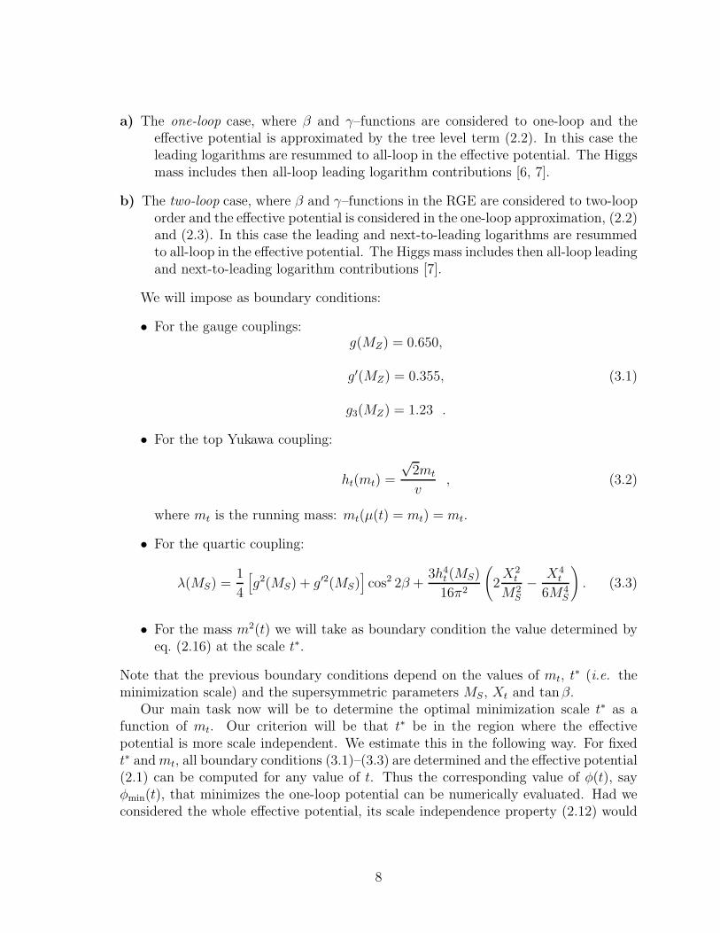
a) The one-loop case, where β and γ–functions are considered to one-loop and theeffective potential is approximated by the tree level term (2.2). In this case theleading logarithms are resummed to all-loop in the effective potential. The Higgsmass includes then all-loop leading logarithm contributions [6, 7].

b) The two-loop case, where β and γ–functions in the RGE are considered to two-looporder and the effective potential is considered in the one-loop approximation, (2.2)and (2.3). In this case the leading and next-to-leading logarithms are resummedto all-loop in the effective potential. The Higgs mass includes then all-loop leadingand next-to-leading logarithm contributions [7].

We will impose as boundary conditions:

• For the gauge couplings:g(MZ) = 0.650,

g′(MZ) = 0.355,

g3(MZ) = 1.23 .

(3.1)

• For the top Yukawa coupling:

ht(mt) =

√2mt

v, (3.2)

where mt is the running mass: mt(µ(t) = mt) = mt.

• For the quartic coupling:

λ(MS) =1

4

[

g2(MS) + g′2(MS)]

cos2 2β +3h4

t (MS)

16π2

(

2X2

t

M2S

− X4t

6M4S

)

. (3.3)

• For the mass m2(t) we will take as boundary condition the value determined byeq. (2.16) at the scale t∗.

Note that the previous boundary conditions depend on the values of mt, t∗ (i.e. theminimization scale) and the supersymmetric parameters MS, Xt and tanβ.

Our main task now will be to determine the optimal minimization scale t∗ as afunction of mt. Our criterion will be that t∗ be in the region where the effectivepotential is more scale independent. We estimate this in the following way. For fixedt∗ and mt, all boundary conditions (3.1)–(3.3) are determined and the effective potential(2.1) can be computed for any value of t. Thus the corresponding value of φ(t), sayφmin(t), that minimizes the one-loop potential can be numerically evaluated. Had weconsidered the whole effective potential, its scale independence property (2.12) would

8

imply that φmin(t)/ξ(t) = 〈φ(t)〉/ξ(t), where 〈φ(t)〉 has been defined in (2.13), is t–independent. Since the one-loop approximation is not exactly scale independent themost appropriate scale is the scale ts for which φmin(t)/ξ(t) has a stationary point, i.e.

d

dt

φmin(t)

ξ(t)

∣

∣

∣

∣

∣

t=ts

= 0. (3.4)

Of course the scale at which (3.4) occurs depends on t∗ and mt, i.e. ts ≡ ts(t∗, mt).

Therefore, for a given value of mt the optimal scale t∗ is defined as

ts ≡ ts(t∗, mt) = t∗, (3.5)

i.e. it is the scale which simultaneously defines the boundary condition (2.16) andagrees with the extremal of the function φmin(t)/ξ(t).

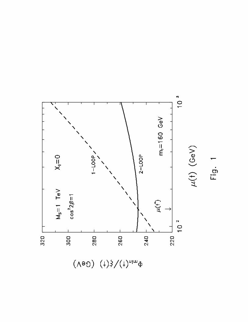
This procedure is illustrated in Fig. 1, where we plot φmin(t)/ξ(t) vs. µ(t) formt = 160 GeV and supersymmetric parameters MS = 1 TeV, Xt = 0, cos2 2β = 1.The solid curve shows the two-loop result whose stationary point satisfies eq. (3.5)and therefore defines the optimal scale t∗. Note that there is no fine tuning in thechoice (3.5) since any point near the stationary point would be equally appropriatebecause the curve φmin(t)/ξ(t) is very flat in that region. We have also shown in Fig. 1the curve φmin(t)/ξ(t) in the one-loop approximation (dashed curve) with µ(t∗) fixedby the two-loop result. We can see that the one-loop curve is much steeper than thetwo-loop curve, which means that the one-loop result, i.e. the tree level potential (2.2)improved by the one-loop RGE, is far from being scale independent at any scale. Thisfeature has also been observed for the MSSM one-loop effective potential [17].

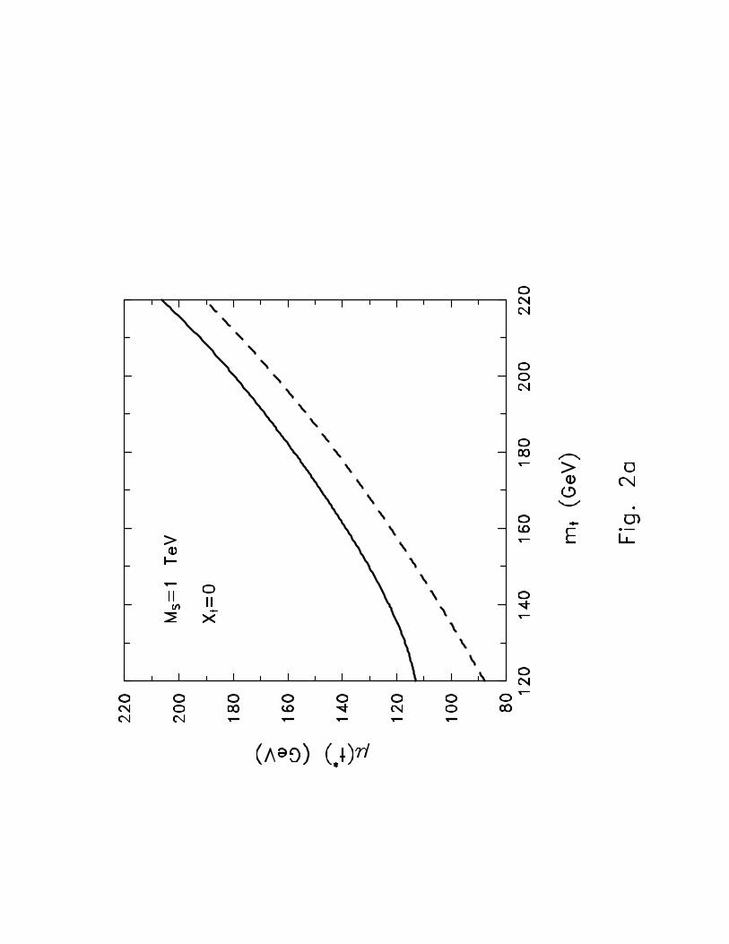
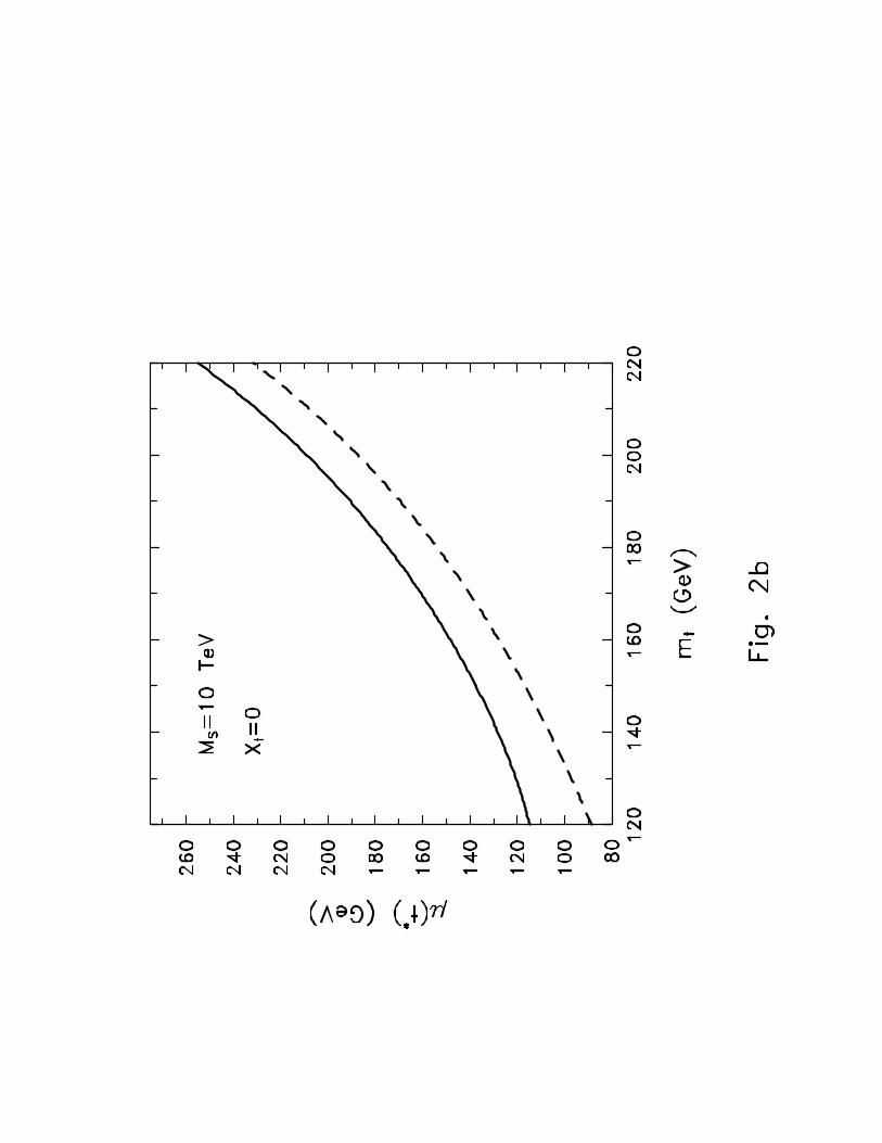
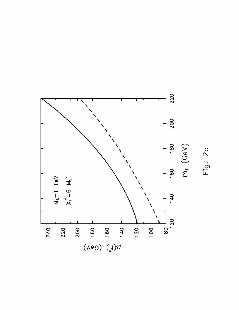
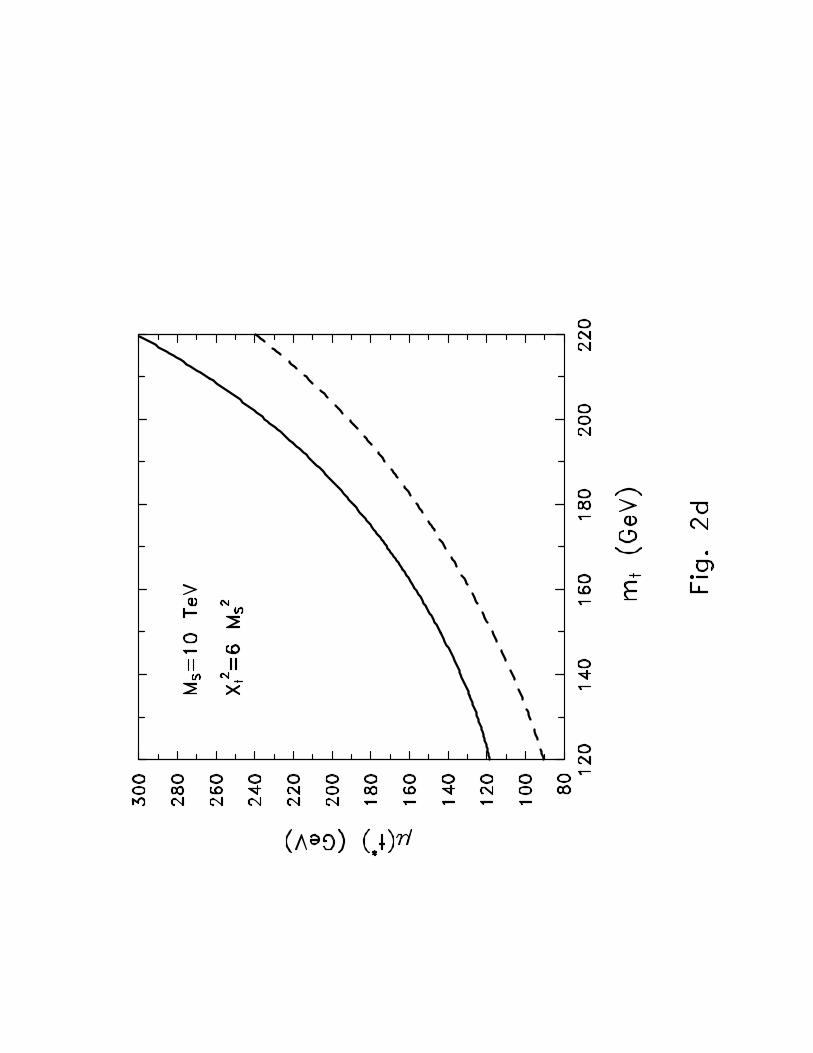
We plot in Figs. 2a,b,c,d, µ(t∗) as a function of mt for the different values of su-persymmetric parameters MS = 1, 10 TeV; X2

t = 0, 6M2S. In all plots the solid curve

corresponds to cos2 2β = 1 and the dashed curve to cos2 2β = 0.Once we have determined µ(t∗) for fixed values of mt and all supersymmetric pa-

rameters, the Higgs running mass mH(t) is given by (2.18), while the mass defined asthe second derivative of the effective potential mH,der(t) is given by (2.19). By definitionboth masses coincide at t∗

mH(t∗) = mH,der(t∗), (3.6)

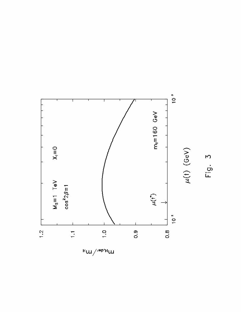
and the ratio mH,der(t)/mH(t) should be equal to one for an exactly scale independenteffective potential. Consistency of our procedure requires the curve mH,der(t)/mH(t) tobe flat in the region where we minimize, i.e. at t∗. In Fig. 3 we plot mH,der(t)/mH(t)for mt = 160 GeV and the values of supersymmetric parameters as in Fig. 1, MS = 1TeV, Xt = 0, cos2 2β = 1. We see that at the point µ(t∗) the curve is in its flat region,though µ(t∗) does not exactly coincide with the extremum of mH,der(t)/mH(t).

Neither mH nor mt are physical masses. They are computed from the effective po-tential, i.e. at zero external momentum, and need to be corrected by the correspondingpolarizations to obtain the propagator pole physical masses. This will be done in sec-tion 4. For the time being, and just to compare with other results in the literature, we

9

will neglect the shift to the physical poles and define the top mass by the boundarycondition (3.2) and the Higgs mass by the usual condition

mH (µ(t) = mH) = mH . (3.7)

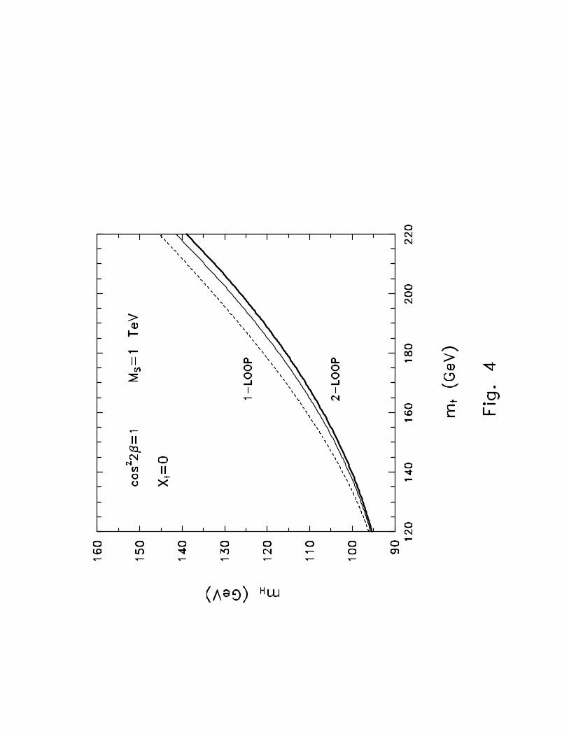
In this way the Higgs mass mH can be unambiguously determined. We plot in Fig. 4mH as a function of mt for the values of supersymmetric parameters MS = 1 TeV,Xt = 0, cos2 2β = 1. The thin solid line corresponds to the two-loop result and thedashed-line corresponds to the one-loop result. (We will disregard for the moment thethick solid line, which corresponds to shifting the running masses to propagator poles.)The main feature that arises from Fig. 4 is that the two-loop corrections are negativewith respect to the one-loop result. This feature is in qualitative agreement with ourprevious two-loop result [5] (where the one-loop corrections to the effective potentialwhere not considered) and with others from different authors [10]. This comparisonwill be done in some detail in section 5.

4 Numerical Results

We will present, in this section, the numerical results on the Higgs mass, evaluatedin the next-to-leading logarithm approximation, as a function of the top quark mass.The running top quark mass mt that we have been using in the previous section wasevaluated at the scale µ(t) = mt, i.e. mt(mt) = mt (see eq.(3.2)). However the runningmass does not coincide with the gauge invariant pole of the top quark propagator Mt.In the Landau gauge the relationship between the running mt and the physical (pole)mass Mt is given by [14]

Mt =

[

1 +4

3

αs(Mt)

π

]

mt(Mt). (4.1)

On the other hand, the running Higgs mass, mH(t), given by eq. (2.18), has a scalevariation

dm2H(t)

dt= 2γm2

H(t). (4.2)

The propagator pole MH is related to the running mass through (see Appendix B)

M2H = m2

H(t) + ReΠ(M2H) − ReΠ(0), (4.3)

where Π(q2) is the (renormalized) self-energy of the Higgs boson. In our calculation(case (b) in section 3) it is enough to compute the Higgs self-energies at the one-looplevel since we are computing the Higgs masses to one-loop. The imaginary part ofΠ(M2

H) − Π(0) contributes to the Higgs width. Assuming MH < 2MW , the Higgs isstable at tree level, and eq. (4.3) reads

M2H = m2

H + Π(M2H) − Π(0). (4.4)

10

The calculation of Π(M2H) − Π(0) is presented in Appendix B. We note that the scale

dependence (at the one-loop level) of mH(t), as provided by (4.2), is cancelled by thescale dependence of Π(M2

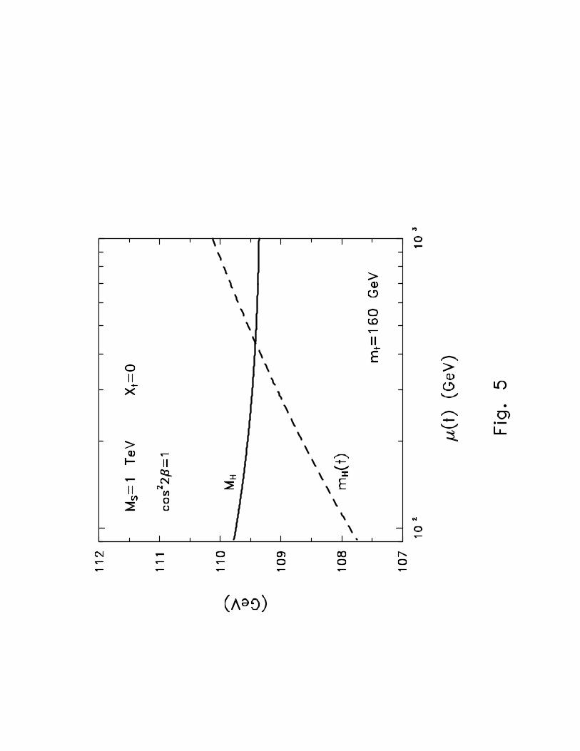
H)−Π(0). The only remaining scale dependence of MH comesfrom two-loop contributions. This feature is exhibited in Fig. 5 where we plot MH inthe range of µ(t) between MS and MZ for mt = 160 GeV and the supersymmetricparameters MS = 1 TeV, Xt = 0, cos2 2β = 1. We can see that MH has a negligiblevariation (∼ 0.5 GeV) between MS and MZ . For the sake of comparison we have alsoplotted the running mass mH(t) whose variation is more appreciable (∼ 2.5 GeV). Thiseffect is more accentuated for larger top masses.

We can see from (4.1) and from Fig. 4 that the effect of considering the pole mass Mt

is negative on the two-loop corrections to the Higgs mass, while the effect of Π(M2H)−

Π(0) is positive (∼ 2 GeV for mt = 160 GeV and ∼ 5 GeV for mt = 215 GeV) thuspartially compensating the effect of (4.1). The global effect is negative and small ascan be seen in Fig. 4. The thick solid line indicates MH as a function of Mt. It is belowthe thin solid line which was the two-loop evaluation of mH as a function of mt. Thecomparison with the one-loop result (dashed line) shows that two-loop corrections arenegative with respect to the one-loop result. Numerically they are small (∼ 1 GeV)for Mt = 120 GeV and larger (∼ 6 − 7 GeV) for Mt = 220 GeV.

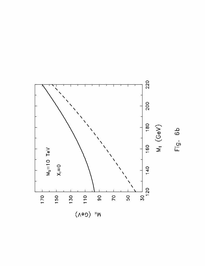
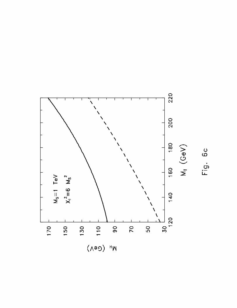
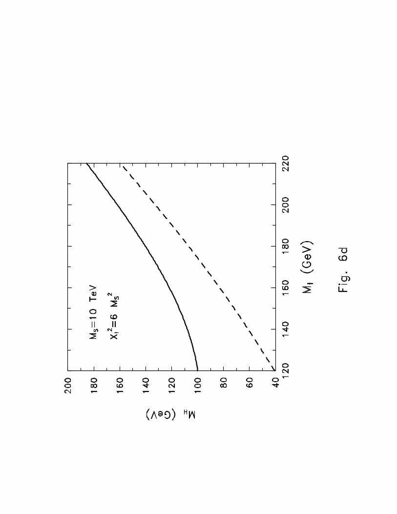
In Fig. 6a,b,c,d we plot MH as a function of Mt for values of supersymmetricparameters MS = 1, 10 TeV; X2

t = 0, 6M2S; cos2 2β = 0, 1. In all cases the solid curve

corresponds to cos2 2β = 1 and the dashed curve to cos2 2β = 0. Notice that thedependence on the mixing parameter Xt is sizeable. In all the figures we have used thelower limit on the top quark mass, Mt > 120 GeV at 95% C.L., from the CDF dileptonchannel [11]. If we use the recent evidence for the top quark production at CDF witha mass Mt = 174 ± 10+13

−12 GeV [11] and the bounds for supersymmetric parametersMS ≤ 1 TeV and maximal threshold correction X2

t = 6M2S, we obtain the absolute

upper bound MH < 140 GeV.The dependence of MH on tanβ is exhibited in Fig. 7 where we fix Mt = 170 GeV

and MS = 1 TeV. The solid curve corresponds to the absolute upper bound for themixing X2

t = 6M2S and the dashed curve to the case of zero mixing. Concerning the

dependence of MH on the stop mixing Xt parameter (or equivalently the stop splitting),we have found it to be sizeable, as can be seen from Figs. 6.

5 Connection with other approaches

Some papers have recently appeared aiming to estimate the mass of the lightest Higgsboson up to next-to-leading order in the MSSM, and with apparently contradictoryresults. In this section we will comment on those papers in the context of our formalismand will exhibit the origin of the disagreements.

In ref. [9] the RG approach was used to estimate the mass of the lightest Higgs boson upto next-to-leading order. The relevant points of their calculation are the following: i)They considered the one-loop correction to the effective potential in the approximation

11

g = g′ = 0, ii) They neglected the wave-function renormalization leading to physicalmasses for the top quark and Higgs boson, iii) They minimized the effective potentialat the scale µ(t∗) = v. In addition they only consider the case of zero stop mixing,Xt = 0.

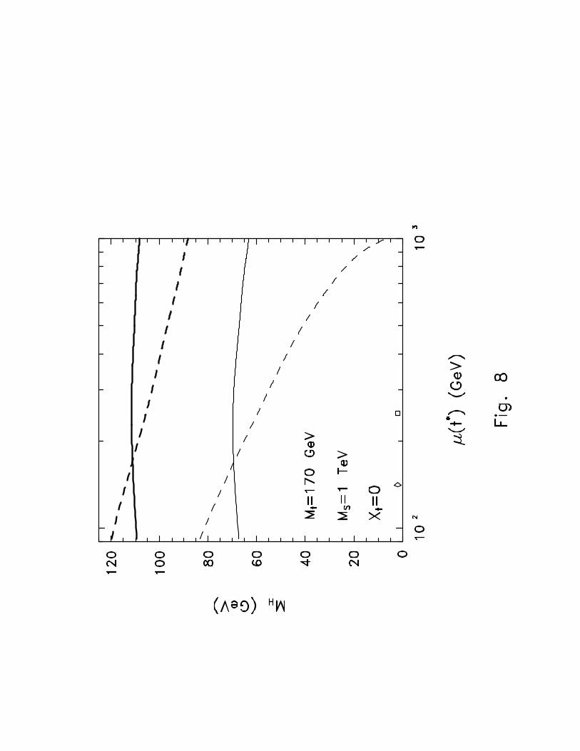
Contrary to our results, they found that the two-loop correction is positive andsizeable with respect to the one-loop result. For instance in the typical case MS = 1TeV, Xt = 0, cos2 2β = 1, they find for mt = 170 GeV the two-loop result mH ∼ 117GeV, while we find for Mt = 170 GeV the two-loop result MH ∼ 111 GeV. We havebeen able to trace back the difference between the two results to the points i)–iii)above. In particular, the authors of ref. [9] find for the same values of the parametersa positive two-loop correction with respect to the one-loop result ∼ 7 GeV while ourtwo-loop result is smaller than the one-loop result by ∼ 3 GeV. To understand theorigin of this discrepancy we have plotted in Fig. 8 the physical Higgs mass MH asa function of the minimization scale µ(t∗) for Mt = 170 GeV, MS = 1 TeV andXt = 0. Thick lines correspond to cos2 2β = 1 and thin lines to cos2 2β = 0. Solidlines represent MH evaluated in the two-loop approximation and dashed lines in theone-loop approximation. Our chosen value of µ(t∗) is indicated in the figure with anopen diamond and that chosen in ref. [9], µ(t∗) = v, with an open square. We cansee that MH evaluated at two-loop is very stable against µ(t∗): it varies ∼ 5 GeVin the whole interval MZ ≤ µ(t∗) ≤ MS and ∼ 2 GeV between the diamond andthe square. However the value of MH evaluated at one-loop is very unstable. In factthe two-loop correction changes from negative at µ(t) = MZ (>

∼ 10%) to positive atµ(t) = MS (>

∼ 20%). In the region of our chosen value of µ(t∗) it is negative and ∼ 3GeV while at µ(t∗) = v it is positive and greater ∼ 7 GeV. Fig. 8 shows that thoughour choice of µ(t∗) is more in agreement with perturbation theory than µ(t∗) = v thedifference is however not important when plotting the physical Higgs mass (which wasnot considered in ref.[9]).

In ref. [10] the diagrammatic and effective potential approaches were used to evaluatethe lightest Higgs mass at two-loop order in the framework of the MSSM. Variousapproximations, like g = g′ = 0 in the effective potential, were used, and only thecase of zero stop mixing, Xt = 0, was considered. Our results agree with those ofref. [10] within less than ∼ 3 GeV. In fact for Mt = 150 GeV, Xt = 0, cos2 2β = 1and MS = 1 TeV (MS = 10 TeV) ref. [10] finds MH ∼ 107 GeV (MH ∼ 110 GeV)while we find from Figs. 6a and 6b MH ∼ 103 GeV (MH ∼ 110 GeV). We considerthis agreement as satisfactory given the approximations used in ref. [10]. The fact thattwo-loop corrections found in ref. [10] are sizeable with respect to the one-loop resultcan be explained as a consequence of the approximation used there to estimate the one-loop result. Taking MS = 10 TeV and Mt = 150 GeV, they found mH = 138 GeV atone-loop using a simple approximation that takes into account only the leading part (∼M4

t log(M2S/M2

t )) of the corrections, as it is common practice in some phenomenologicalanalysis. Actually, a slightly more sofisticated approximation (as the one labelled 1β intheir paper) or the one-loop result obtained by a numerical integration of the RGE (as

12

in our approach) gives mH ∼ 115 GeV (both methods agree up to a difference ∼ 2− 3GeV due to subleading effects, such as those provided by considering gauge couplingsin the effective potential) for the above mentioned values of the parameters. This hasto be compared with the two-loop result MH ∼ 110 GeV and shows that the net effectof two-loop corrections is indeed negative and small6.

Finally bounds on the lightest Higgs mass have been recently analyzed in ref. [18]in the context of models with Yukawa unification. The results of ref. [18] are presentedin the one-loop approximation. They choose MZ as the minimization scale and findlarger bounds than in previous estimates. For instance it is found, for Mt = 170GeV and any value of the supersymmetric parameters such that MS < 1 TeV, thatMH

<∼ 102 GeV. We have tried to reproduce their results using our formalism. In fact,

their solution for small tan β is close to the fixed point solution where tan β and mt

are related through [19]

mt = (196 GeV)[1 + 2(α3(MZ) − 0.12)] sin β. (5.1)

Now, fixing MS = 1 TeV and maximal mixing7 X2t = 6M2

S we find, for Mt = 170 GeVthat tanβ = 1.74 from (5.1) and MH ∼ 99 GeV if we fix µ(t∗) = MZ , in agreementwith the result of ref. [18]. However this large value of MH is a clear consequenceof the chosen minimization scale where two-loop corrections are very large. In factfor µ(t∗) = MZ our two-loop result gives MH ∼ 85 GeV. Moving to the region whereperturbation theory is more reliable, as we have done along this paper, we would obtainthe final two-loop result, MH ∼ 86 GeV. We have plotted in Fig. 9 MH as a functionof Mt for MS = 1 TeV and tan β, determined from (5.1), corresponding to the fixedpoint solution. The solid (dashed) line corresponds to the case of maximal mixing,X2

t = 6M2S (zero mixing, Xt = 0).

6 Conclusions

We have computed in this paper the upper bounds on the mass of the lightest Higgsboson in the MSSM including leading and next-to-leading logarithm radiative correc-tions. We have used an RG approach by means of a careful treatment of the effectivepotential in the SM, assuming that supersymmetry is decoupled from the SM, whichwe have shown to be an excellent approximation for MS

>∼ 1 TeV or even much less.

Our results have covered the whole parameter space of supersymmetric parameters; in

6Notice that the results of ref. [10] only contain one- and two-loop leading and next-to-leadingcontributions to the Higgs mass while, as we have noticed before, our calculation of the Higgs massincludes leading and next-to-leading contributions to all-loop. This effect can be important for thecase of large logarithms. We thank R. Hempfling for a discussion on this point.

7An interesting result that can be confirmed from ref. [18] (see Fig. 10 in that paper) is that themaximal threshold limit is compatible with the non-existence of color breaking minima, as we alreadynoted. For that reason removing the color breaking minima of the distribution plotted in Fig. 7 doesnot change the upper bound on the Higgs mass.

13

fact, when we refer to the MSSM, we simply mean the supersymmetric version of theSM with minimal particle content. We have also included QCD radiative correctionsto the top quark mass, which gives a negative contribution to the Higgs mass as afunction of the physical (pole) top mass Mt, and electroweak radiative corrections tothe Higgs mass MH , Π(M2

H)−Π(0), providing a positive contribution to MH and par-tially cancelling the former ones. Therefore the balance of including the contribution ofQCD and electroweak self-energies to the quark and Higgs masses is negative and small(<∼ 2% for Mt < 200 GeV). We also made a reliable estimate of the total uncertainty

in the final results, which turns out to be quite small (∼ 2 GeV ).Concerning the numerical results, we have found in particular that for Mt ≤ 190

GeV, MS ≤ 1 TeV and any value of tanβ we have MH < 120 GeV for Xt = 0, andMH < 140 GeV for X2

t = 6M2S (maximal threshold effect). We have also applied our

calculation to a particularly appealing scenario, namely the assumption that the tophas the Yukawa coupling in its infrared fixed point. Then, the bounds are much morestringent. E.g. for Mt = 170 GeV, MS ≤ 1 TeV and X2

t = 6M2S, we find MH ≤ 86

GeV.Two papers have recently tried to incorporate radiative corrections to the Higgs

mass up to the next-to-leading order and with qualitatively different results. In ref. [9],using the RG approach, positive, and large next-to-leading corrections with respect tothe one-loop results were found. In ref. [10], using diagrammatic and effective potentialmethods in a particular MSSM as well as various approximations, it was found thattwo-loop corrections are also sizeable, but negative with respect to the one-loop result!

Using the RG approach, as ref. [9], we have found (unlike in ref. [9]) that two-loopcorrections are negative with respect to the one-loop result. We have traced back theorigin of this disagreement in their choice of the minimization scale. Furthermore theauthors of ref. [9] neglected various effects (as the contribution of gauge bosons to theone–loop effective potential, or the wave function renormalization of top quark andHiggs boson) and considered only the case with zero stop mixing.

On the other hand, we have found that the abnormal size of the two-loop correctionsobtained in [10] is a consequence of an excesively rough estimate of the one-loop result,but we are in agreement with their final two-loop result. In fact our two-loop resultsdiffer from those of ref. [10] by less than 3%. Also our results show a large sensitivityof the Higgs mass to the stop mixing parameter.

Finally we would like to comment briefly on the generality of our results. Aswas already stated, we are assuming average squark masses M2

S ≫ M2Z , and that all

supersymmetric particle masses are >∼ MS. If we relax the last assumption, i.e. if some

supersymmetric particles were much lighter, the value of the quartic coupling at MS

(see eq. (1.3)) would be slightly increased and, correspondingly, our bounds wouldbe slightly relaxed. We have made an estimate of this effect. Assuming an extremecase where all gauginos, higgsinos and sleptons have masses ∼ MZ , we have found forMS = 1 TeV and cos2 2β = 1 an increase of the Higgs mass ∼ 2%. For values of tan βclose to one (as those appearing in infrared fixed point scenarios) the correspondingeffect is negligible. On the other hand, our numerical results have been computed

14

for MS ≥ 1 TeV. For values of MS ≤ 1 TeV the bounds on the lightest Higgs massare lowered. Hence, in this sense, all our results can be considered as absolute upperbounds.

Acknowledgements

We thank R. Hempfling and S. Peris for illuminating discussions. We also thank M.Carena, G. Kane, M. Mangano, N. Polonsky, S. Pokorski, A. Santamarıa, C. Wagnerand F. Zwirner for useful discussions and comments.

Appendix A

We comment here on the origin and size of threshold contributions to the quarticcoupling of the SM, λ, at the supersymmetric scale. We also evaluate the effectiveD=6 operators that are relevant for the Higgs potential, showing that for MS ≥ 1 TeVthey are negligible.

As it is well known, the one-loop correction to the MSSM effective potential isdominated by the stop contribution

V MSSM1 =

3

32π2

m41

[

logm2

1

Q2− 3

2

]

+ m42

[

logm2

2

Q2− 3

2

]

(A.1)

where m1, m2 are the two eigenvalues of the stop mass matrix. In a good approxima-tion:

m21,2 = M2

S + h2tH2 ± htH2Xt (A.2)

where M2S is the soft mass of the stops (we are assuming here that this is the same for

the left and the right stops, which is a correct approximation since the RGE of bothmasses are dominated by the same QCD term); ht is the top Yukawa coupling in theMSSM and Xt = At + µ cotβ gives the mixing between stops (At is the coefficient ofthe soft trilinear scalar coupling involving stops and µ is the one of the usual bilinearHiggs term in the superpotential). Notice also that MS is basically the average of thetwo stop masses, which is a reasonable choice for the supersymmetric scale when oneis dealing with the Higgs potential, as it is our case. Thus we identify the scale Q atwhich we are evaluating the threshold effects with MS.

Now it is straightforward to obtain from (A.1) the contribution to the H4 operator(recall that H is the SM Higgs doublet given by eq.(1.2)). That is

3

32π2

(

2X2t

M2S

)

h4t −

(

X4t

6M2S

)

h4t

H4 , (A.3)

where have redefined ht to be the usual top Yukawa coupling in the SM. This gives athreshold contribution to the SM quartic coupling

∆λ =3h4

t

16π2

X2t

M2S

(

2 − X2t

6M2S

)

. (A.4)

15

Alternatively, eq. (A.4) can be obtained diagrammatically from two kinds of dia-grams exchanging stops (see the first paper of ref. [4]). Both methods give the sameresult.

It is worth noticing that (A.4) has a maximum for X2t = 6M2

S, which means thatthe threshold effect cannot be arbitrarily large. Note also that X2

t = 6M2S is barely

consistent with the bound from color conserving minimum [13], so the case of maximalthreshold represents an extreme situation.

Analogously, we can obtain from (A.1) the relevant effective D=6 operators, i.e.

those proportional to H6. These turn out to be

3

32π2

(

2

3M2S

)

−(

X2t

M4S

)

+

(

X4t

3M6S

)

−(

X6t

30M8S

)

h6t H

6 , (A.5)

which could also be obtained diagrammatically from four kinds of diagrams exchangingstops. It is easy to see that (A.5) produces negligible modifications in the process ofelectroweak breaking and in the Higgs mass. For example, for MS = 1 TeV andmaximal threshold in (A.4), i.e. X2

t = 6M2S, (A.5) gives modifications in the Higgs

mass suppressed by a factor ∼ 1/150 with respect to those induced by (A.4). This alsomeans that, regarding the Higgs potential, it is safe to decouple the MSSM from theSM for MS = 1 TeV or even substantially smaller.

Appendix B

In this Appendix we shall discuss in more detail the relation between the running massof the Higgs boson, extracted from the effective potential, and the physical Higgs massand give the complete expression for the latter.

The physical mass of the Higgs boson field MH is defined as the pole of the prop-agator and it is both renormalization scheme and gauge (if calculated at all orders ofperturbation) independent.

We start with the Lagrangian

L =1

2(∂φ0)

2 − 1

2m2

0φ20 + . . .

=1

2(∂φR)2 − 1

2m2

Rφ2R +

1

2δZH (∂φR)2 − 1

2δm2φ2

R + . . . , (B.1)

where φ0 and φR = Z−1/2H φ0 = (1 + δZH)−1/2φ0 are the bare and renormalized Higgs

fields, and m0 and mR are the bare and renormalized masses. With this conventionm2

0 = m2R + δm2 − δZHm2

R. Denoting by Γ0 (ΓR) the inverse of the one-loop correctedbare (renormalized) propagator, we have

ΓR(p2) = ZHΓ0(p2) = ZH

[

p2 − m2R − δm2 + δZHm2

R − Π0(p2)]

= p2 + δZHp2 −(

m2R + δm2

)

− Π0(p2) , (B.2)

16

where Π0(p2) is the (unrenormalized) self-energy of the Higgs boson field and in the

last equality we have neglected higher order terms in the perturbative expansion. Therenormalized self-energy is defined as

ΠR(p2) = Π0(p2) + δm2 − δZHp2. (B.3)

ThusΓR(p2) = p2 −

(

m2R + ΠR(p2)

)

. (B.4)

Consequently, the physical (pole) mass, M2H , satisfies the relation

M2H = m2

R + ΠR(p2 = M2H) . (B.5)

On the other hand, the running mass m2H , defined as the second derivative of the

renormalized effective potential (see eqs. (2.17) and (2.18)), is given by

m2H =

∂2Veff

∂φ2= −ΓR(p2 = 0) = m2

R + ΠR(p2 = 0) . (B.6)

Comparing (B.5) and (B.6) we have

M2H = m2

H + ∆Π, (B.7)

where we have defined (we drop the subscript R from ΠR)

∆Π ≡ Π(p2 = M2H) − Π(p2 = 0). (B.8)

Note that m2H defined in (B.6) is renormalization scheme dependent, as Veff is, while

M2H is not. In particular, in eq.(B.7) both m2

H and ∆Π depend on the renormalizationscale µ in such a way that M2

H results to be scale independent (at least to O(h)). Infact, from eq. (B.3) and the definition

γ =1

2

d log ZH

d log µ(B.9)

we easily obtaind∆Π

d log µ= −2γM2

H (B.10)

which cancels the scale dependence of m2H (see eq.(4.2)).

We now want to give the complete expression for the physical mass M2H . The

quantity ∆Π in the Landau gauge is given by the sum of the following terms

∆Π = ∆Πtt (top contribution)

+ ∆ΠW±W∓ + ∆ΠZ0Z0

+ ∆ΠW±χ∓ + ∆ΠZ0χ3(gauge and Goldstone bosons contribution)

+ ∆Πχ±χ∓ + ∆Πχ3χ3

+ ∆ΠHH (pure scalar bosons contribution). (B.11)

17

In eq. (B.11) we have taken into account only the contribution from the heaviestfermion, the top, and indicated by χ± and χ3 the charged and the neutral Goldstonebosons, respectively.

The complete expression for the different contributions to ∆Π calculated in the MSscheme is, for MH < 2MW :

i) Top contribution:

∆Πtt =3h2

t

8π2

−2M2t

[

Z

(

M2t

M2H

)

− 2

]

+1

2M2

H

[

logM2

t

µ2+ Z

(

M2t

M2H

)

− 2

]

. (B.12)

ii) Gauge bosons and Goldstone bosons contribution:

∆ΠW±W∓ + ∆ΠZ0Z0 + ∆ΠW±χ∓ + ∆ΠZ0χ3

=g2M2

W

8π2

(

I(1)W + I

(2)W +

M2H

2I

(3)W − M2

HI(4)W

+M2

H

4I

(5)W − M4

H

2I

(6)W

)

− 1

2

g2M2H

16π2

(

I(7)W (µ2) + I

(8)W (µ2)

)

+1

2

g2M4H

16π2I

(9)W +

1

2

MW → MZ

g2 → g2 + g′2

, (B.13)

where all the masses in the above expression have to be understood as the physicalones. The I i

W (i = 1, ...., 9) functions read

I1W =

∫ 1

0dx log

[

1 − M2H

M2W

x(1 − x) − iǫ

]

= Z

(

M2W

M2H

)

− 2,

I2W =

∫ 1

0

∫ 1

0dxdy y log

[

1 − M2H

M2W

y(1 − y)

(1 − xy)− iǫ

]

= −11

12− 1

6

M2W

M2H

+1

6

(

4 − M2H

M2W

)

Z

(

M2W

M2H

)

+1

6

(M2H − M2

W )3

M4HM2

W

log

(

1 − M2H

M2W

)

,

I3W =

∫ 1

0

∫ 1

0dxdy

y3

M2W (1 − xy) − M2

Hy(1− y) − iǫ=

5

6

1

M2H

+1

3

M2W

M4H

+1

3M2H

(

M2H

M2W

− 1

)

Z

(

M2W

M2H

)

+1

3M2W

(

M6W

M6H

− 1

)

log

(

1 − M2H

M2W

)

,

I4W =

∫ 1

0

∫ 1

0dxdy

y2

M2W (1 − xy) − M2

Hy(1− y) − iǫ

=1

2

1

M2H

+1

2M2W

Z

(

M2W

M2H

)

+1

2M2W

(

M4W

M4H

− 1

)

log

(

1 − M2H

M2W

)

,

18

I5W =

∫ 1

0

∫ 1

0

∫ 1

0dxdydz

z(1 − z)

M2W (1 − y − z(x − y)) − M2

Hz(1 − z) − iǫ

= −1

3

1

M2H

+1

6M2W

(

4 − M2H

M2W

)

Z

(

M2W

M2H

)

+(M2

H − M2W )

3

3M4HM4

W

log

(

1 − M2H

M2W

)

− 1

6

M2H

M4W

logM2

H

M2W

+iπ

6

M2H

M4W

,

I6W =

∫ 1

0

∫ 1

0

∫ 1

0dxdydz

z3(1 − z)

[M2W (1 − y − z(x − y)) − M2

Hz(1 − z) − iǫ]2

= −2

3

1

M4H

+1

3M2W M2

H

(

1 − M2H

M2W

)

Z

(

M2W

M2H

)

+(M2

H − M2W )

3

3M6HM4

W

log

(

1 − M2H

M2W

)

+1

3M4W

log

(

1 − M2H

M2W

)

−1

3

M2W

M6H

log

(

1 − M2H

M2W

)

+1

3M4W

logM2

W

M2H

+iπ

3

1

M4W

,

I7W =

∫ 1

0dx(1 + 2x) log

[

M2W x − M2

Hx(1 − x) − iǫ

µ2

]

= −4 + 2 logM2

W

µ2+

M2W

M2H

+

(

M4W

M4H

− 3M2

W

M2H

+ 2

)

log

(

1 − M2H

M2W

)

,

I8W =

∫ 1

0dx log

[

M2W x − iǫ

µ2

]

= −1 + logM2

W

µ2,

I9W =

∫ 1

0

∫ 1

0dxdy

1

M2Wx − M2

Hy − iǫ

=

(

1

M2W

− 1

M2H

)

log

(

1 − M2H

M2W

)

+1

M2W

logM2

W

M2H

+iπ

M2W

, (B.14)

where Z(x) is the function

Z(x) =

2A tan−1(1/A), if x > 1/4A log [(1 + A)/(1 − A)] , if x < 1/4

A ≡ |1 − 4x|1/2. (B.15)

The terms containing the factor log(1−M2H/M2

W,Z) develop an imaginary part in theregion MW,Z < MH < 2MW corresponding to the unphysical decays H → W±χ∓, Z0χ3.However, this imaginary part, along with the whole factor log(1−M2

H/M2W,Z), cancels

in (B.13). In fact, using (B.14), (B.13) can be written as:

∆ΠW±W∓ + ∆ΠZ0Z0 + ∆ΠW±χ∓ + ∆ΠZ0χ3

=g2M2

W

8π2

[

−3 +5

4

M2H

M2W

+1

2

(

3 − M2H

M2W

+M4

H

4M4W

)

Z

(

M2W

M2H

)

− M4H

8M4W

logM2

H

M2W

19

− 3M2H

4M2W

logM2

W

µ2+

iπ

8

M2H

M2W

]

+1

2

MW → MZ

g2 → g2 + g′2

. (B.16)

There is also an explicit imaginary part in (B.16) giving rise to

Im(∆ΠW±W∓ + ∆ΠZ0Z0 + ∆ΠW±χ∓ + ∆ΠZ0χ3) =

3g2

128π

M4H

M2W

(B.17)

which will also cancel, as we will see.iii) Pure scalar bosons contribution: the contribution to ∆Π coming from the pure

scalar sector deserves more attention and we want to discuss it in more details.It is well-known that in the Landau gauge the Goldstone bosons χ’s do have a field

dependent mass mχ(φ) = −m2+λφ2/2 which vanishes at the minimum of the potentialVeff(φ). As a consequence, the running mass mH presents an infrared logarithmicdivergence when Goldstone bosons are included in the effective potential Veff(φ). Onthe other hand, the physical mass MH must be finite and gauge independent, so thedivergent contribution coming from the Goldstone bosons to m2

H must be cancelled byan equal (and opposite in sign) contribution of the same excitations to ∆Π. To seeit explicitly, one can imagine the Goldstone bosons to have a fictitious mass mχ andcalculate their contribution ∆m2

H to the running square mass m2H . It is not difficult to

see that this contribution from the effective potential is

∆m2H =

3

128π2

g2M4H

M2W

[

3 logM2

H

µ2(t⋆)+ log

m2χ

µ2(t⋆)

]

+ O(h2), (B.18)

where the scale µ(t⋆) is defined in the text. On the other hand, the contribution to∆Π from the pure scalar sector reads

∆ΠHH + ∆Πχ±χ∓ + ∆Πχ3χ3=

3

128π2

g2M4H

M2W

[

π√

3 − 8 + Z

(

m2χ

M2H

)

− iπ

]

, (B.19)

where the last term comes from the Feynman diagrams involving Goldstone bosons.The explicit imaginary part in (B.19) would correspond to the unphysical decays H →χ±χ∓, χ3χ3 and cancels against eq. (B.17). Expanding now the function Z

(

m2χ/M2

H

)

around m2χ = 0 one can easily show that the logarithmic divergence in ∆m2

H disappearsand the final result for the pure scalar bosons contribution to ∆M2

H is finite and givenby

∆M2H =

3

128π2

g2M4H

M2W

[

π√

3 − 8 + 4 logM2

H

µ2(t⋆)

]

. (B.20)

Finally it is worth making a couple of comments. First, we have included the purescalar bosons sector in ∆Π for the sake of completeness, but now one is no longerallowed to compare the physical mass given in eq. (B.7) with the running mass sincethe latter (see eq. (B.18)) is not well defined when Goldstone bosons are taken intoaccount. Secondly, there is no scale dependence in the last expression (B.20) (the scaleµ(t⋆) is fixed (see the text)), in agreement with the fact that the λ-dependence of theanomalous dimension γ of the Higgs field arises at two-loop.

20

References

[1] Z. Kunszt and W.J. Stirling, Phys. Lett. B262 (1991) 54.

[2] Y. Okada, M. Yamaguchi and T. Yanagida, Prog. Theor. Phys. 85 (1991) 1;J. Ellis, G. Ridolfi and F. Zwirner, Phys. Lett. B257 (1991) 83 and B262 (1991)477;R. Barbieri and M. Frigeni, Phys. Lett. B258 (1991) 395;D. Pierce, A. Papadopoulos and S. Johnson, Phys. Rev. Lett. 68 (1992) 3678.

[3] H. E. Haber and R. Hempfling, Phys. Rev. Lett. 66 (1991) 1815;A. Yamada, Phys. Lett. B263 (1991) 233;A. Brignole, Phys. Lett. B281 (1992) 284;P. H. Chankowski, S. Pokorski and J. Rosiek, Phys. Lett. B274 (1992) 191.

[4] Y. Okada, M. Yamaguchi and T. Yanagida, Phys. Lett. B262 (1991) 54;R. Barbieri, M. Frigeni and F. Caravaglios, Phys. Lett. B258 (1991) 167;H. E. Haber and R. Hempfling, Phys. Rev. D48 (1993) 4280.

[5] J. R. Espinosa and M. Quiros, Phys. Lett. B266 (1991) 389.

[6] B. Kastening, Phys. Lett. B283 (1992) 287.

[7] M. Bando, T. Kugo, N. Maekawa and H. Nakano, Phys. Lett. B301 (1993) 83.

[8] C. Ford, D. R. T. Jones, P. W. Stephenson and M. B. Einhorn, Nucl. Phys. B395(1993) 17.

[9] J. Kodaira, Y. Yasui and K. Sasaki, Hiroshima preprint HUPD-9316, YNU-HEPTh-93-102 (November 1993).

[10] R. Hempfling and A. H. Hoang, Phys. Lett. B331 (1994) 99.

[11] F. Abe et al., CDF Collaboration, preprint FERMILAB-PUB-94/097-E andPhys. Rev. Lett. 73 (1994) 225.

[12] G. t’Hooft and M. Veltman, Nucl. Phys. B61 (1973) 455;W. A. Bardeen, A. J. Buras, D. W. Duke and T. Muta, Phys. Rev. D18 (1978)3998.

[13] J. M. Frere, D. R. T. Jones and S. Raby, Nucl. Phys. B222 (1983) 11; C. Kounnas,A.B. Lahanas, D.V. Nanopoulos and M. Quiros, Nucl. Phys. B236 (1984) 438;J.-P. Derendinger and C. A. Savoy, Nucl. Phys. B237 (1984) 307; J. A. Casas, A.Lleyda and C. Munoz, to appear.

[14] N. Gray, D. J. Bradhurst, W. Grafe and K. Schilcher, Z. Phys. C48 (1990) 673.

[15] S. Peris, Mod. Phys. Lett. 16 (1991) 1505.

21

[16] H. Arason et al., Phys. Rev. D46 (1992) 3945.

[17] G. Gamberini, G. Ridolfi and F. Zwirner, Nucl. Phys. B331 (1990) 331; B. deCarlos and J. A. Casas, Phys. Lett. B309 (1993) 320

[18] P. Langacker and N. Polonsky, preprint UPR-0594T (February 1994).

[19] V. Barger, M. S. Berger, P. Ohmann and R. J. N. Phillips, Phys. Lett. B314(1993) 351; M. Carena and C. Wagner, CERN preprint CERN–TH.7321/94.

22

Figure Captions

Fig. 1 Plot of φmin(t)/ξ(t) as a function of µ(t) for mt = 160 GeV and supersymmet-ric parameters: MS = 1 TeV, Xt = 0, cos2 2β = 1. The solid (dashed) curvecorresponds to the two loop (one-loop) approximation.

Fig. 2 Plot of µ(t∗) as a function of mt for cos2 2β = 1 (solid line) and cos2 2β = 0(dashed line) and values of supersymmetric parameters: a) MS = 1 TeV, Xt = 0;b) MS = 10 TeV, Xt = 0; c) MS = 1 TeV, X2

t = 6M2S; and d) MS = 10 TeV,

X2t = 6M2

S.

Fig. 3 Plot of mH,der(t)/mH(t) as a function of µ(t) for mt = 160 GeV and the super-symmetric parameters: MS = 1 TeV, Xt = 0, cos2 2β = 1.

Fig. 4 The thin lines correspond to mH as a function of mt in the two-loop (solid)and one-loop (dashed) approximation for supersymmetric parameters: MS = 1TeV, Xt = 0, cos2 2β = 1. The thick solid line is the plot of MH , (4.3), as afunction of Mt, (4.1), in the two-loop approximation and for the same values ofthe supersymmetric parameters.

Fig. 5 Plot of the physical, MH (solid curve), and running, mH (dashed curve) Higgsmass as a function of the scale µ(t) for supersymmetric parameters MS = 1 TeV,Xt=0, cos2 2β = 1.

Fig. 6 Plot of MH as a function of Mt for cos2 2β = 1 (solid line) and cos2 2β = 0(dashed line) and values of supersymmetric parameters: a) MS = 1 TeV, Xt = 0;b) MS = 10 TeV, Xt = 0; c) MS = 1 TeV, X2

t = 6M2S; and d) MS = 10 TeV,

X2t = 6M2

S.

Fig. 7 Plot of MH as a function of tanβ for Mt = 170 GeV and MS = 1 TeV. Thesolid (dashed) curve corresponds to the X2

t = 6M2S (Xt = 0) case.

Fig. 8 Plot of MH as a function of µ(t∗) for Mt = 170 GeV, MS = 1 TeV, Xt = 0.Solid (dashed) lines are the two-loop (one-loop) approximation, thick (thin) linescorrespond to cos2 2β = 1 (cos2 2β = 0).

Fig. 9 Plot of MH as a function of Mt for MS = 1 TeV and tanβ determined fromthe fixed point condition (5.1). The solid line corresponds to maximal mixing,X2

t = 6M2S and the dashed line to Xt = 0.

23

This figure "fig1-1.png" is available in "png" format from:

http://arXiv.org/ps/hep-ph/9407389v1












































Documents

The lightest Higgs boson mass in the Minimal ... · The lightest Higgs boson mass in the Minimal Supersymmetric Standard Model∗ J.A. Casas1, 2, J. R. Espinosa †, M. Quir´os2