Heriot-Watt University Research Gateway

Heriot-Watt University

The Lifetime Performance Prediction of Fractured Horizontal Wells in Tight ReservoirsMoradi DowlatAbad, Mojtaba; Jamiolahmady, Mahmoud

Published in:Journal of Natural Gas Science and Engineering

DOI:10.1016/j.jngse.2017.02.041

Publication date:2017

Document VersionPeer reviewed version

Link to publication in Heriot-Watt University Research Portal

Citation for published version (APA):Moradi DowlatAbad, M., & Jamiolahmady, M. (2017). The Lifetime Performance Prediction of FracturedHorizontal Wells in Tight Reservoirs. Journal of Natural Gas Science and Engineering, 42, 142–156. DOI:10.1016/j.jngse.2017.02.041

General rightsCopyright and moral rights for the publications made accessible in the public portal are retained by the authors and/or other copyright ownersand it is a condition of accessing publications that users recognise and abide by the legal requirements associated with these rights.

If you believe that this document breaches copyright please contact us providing details, and we will remove access to the work immediatelyand investigate your claim.

Download date: 17. Jul. 2018

Accepted Manuscript

The lifetime performance prediction of fractured horizontal wells in tight reservoirs

Mojtaba MoradiDowlatabad, Mahmoud Jamiolahmady

PII: S1875-5100(17)30094-X

DOI: 10.1016/j.jngse.2017.02.041

Reference: JNGSE 2094

To appear in: Journal of Natural Gas Science and Engineering

Received Date: 20 November 2016

Revised Date: 11 January 2017

Accepted Date: 21 February 2017

Please cite this article as: MoradiDowlatabad, M., Jamiolahmady, M., The lifetime performanceprediction of fractured horizontal wells in tight reservoirs, Journal of Natural Gas Science & Engineering(2017), doi: 10.1016/j.jngse.2017.02.041.

This is a PDF file of an unedited manuscript that has been accepted for publication. As a service toour customers we are providing this early version of the manuscript. The manuscript will undergocopyediting, typesetting, and review of the resulting proof before it is published in its final form. Pleasenote that during the production process errors may be discovered which could affect the content, and alllegal disclaimers that apply to the journal pertain.

MANUSCRIP

T

ACCEPTED

ACCEPTED MANUSCRIPT

The Lifetime Performance Prediction of Fractured Horizontal Wells in Tight

Reservoirs

Mojtaba MoradiDowlatabad, Mahmoud Jamiolahmady, Heriot-Watt University

Abstract

Multiple fractured horizontal wells (MFHWs) are recognised as the most effective

stimulation technique to improve recovery from tight and shale gas assets. The performance

of MFHWs depends on series of flow regimes developed during production. Understanding

of the complex flow behaviour and the proper interpretation of these flow regimes are

necessary to obtain information about the reservoir and to predict the performance of these

wells.

There are several models available for simulating the early transient linear flow behaviour in

unconventional reservoirs. However, they involve over-simplifying assumptions about the

hydraulic fracture geometry and the reservoir. Furthermore, these models fail to appropriately

consider the compound linear flow regime, the interference effect and/or the transitional

periods in between different flow regimes that are expected to be important in such low

permeability formations.

In this paper, the aim is to investigate the key characteristics of the transient (unsteady-state)

flow periods and accordingly propose a practically attractive tool for performance prediction

of the MFHWs in tight reservoirs. To achieve this objective, first, series of simulated well test

data are discussed to identify the key practical flow regimes that can be expected for various

practical MFHWs designs with different fracture spacing, length of fractures etc. Following

this investigation, new analytical models are proposed to predict the performance of MFHWs

under different dominant transient flow regimes.

Moreover, integrating the new models with the pseudo steady state (PSS) productivity index

formulation proposed previously by the authors, a new approach is presented that covers the

identified flow regimes, i.e. the formation linear, the compound linear and PSS flow regimes

and the transition periods in between. The outcome of this study can be used for tasks such as

well testing, production performance analysis, forecasting and optimisation of MFHWs

design.

1. Introduction

Conventionally the formations with permeability varying between 1µD and 0.1 mD are

classified as tight reservoirs. In these reservoirs, enlarged drainage area by the horizontal well

MANUSCRIP

T

ACCEPTED

ACCEPTED MANUSCRIPT

2

with multiple transvers fractures increases the well productivity significantly. This is why

multiple fractured horizontal wells are considered as the most effective stimulation technique

to improve recovery from such low permeability reservoirs. Understanding of the complex

flow behaviour and predicting the performance of these wells are vital. The available

production analysis methods that have, so far, been used for unconventional reservoirs are: 1)

Straight-line (or flow-regime) analysis, 2) Type-curve, 3) Empirical, 4) Semi-analytical and

numerical simulation and 5) Hybrid (e.g. analytical and empirical) methods.

Many researches contributed to the understanding of the early transient flow in

unconventional reservoirs using straight-line analysis methods (Gringarten and Ramey 1973,

Wattenbarger et al. 1998, Lee and Holditch 1981, Lee and Brockenbrough 1986, Arevalo-

Villagran et al. 2001).

Nobakht et al. (2010) presented a hybrid approach to forecast production from shale

reservoirs by applying analytical equations for the transient period and using hyperbolic

decline curves for the boundary dominated flow period.

Analytical modelling has been typically used to a) generate type-curves; b) characterise the

system; and c) to generate production forecasts. Meyer et al. (2010) presented an analytical

methodology to predict performance of MFHWs based on trilinear (Lee and Brockenbrough

1986) and pseudo steady-state resistivity models (Meyer and Jacot 2005) of fluid flow

towards vertical fractures in shale reservoirs. Azari et al. (1990) presented constant-pressure,

semi-analytical solutions using the Duhamel’s theorem and Laplace transformations for the

constant-rate solution, when considering only bilinear, linear and pseudo-radial flow regimes.

Furthermore, in many of these models are based on over-simplifying assumptions about the

hydraulic fracture geometry and the reservoir. For example, some assume that all fractures

must extend to reservoir boundaries. Such assumptions cause, for example, the linear flow to

be immediately followed by a boundary-dominated flow, which means they lack to

appropriately consider the compound linear flow regime, the interference effect and/or the

transitional periods in between different flow regimes that are expected to be dominant in

such low permeability formations. In the following, first, analysis of simulated well test data

is presented to identify the key practical flow regimes that can be expected for various

practical MFHWs designs. Following this investigation, new analytical models are proposed

to predict the performance of MFHWs under various dominant transient flow regimes.

Finally, integrating the new models with the pseudo steady state (PSS) productivity index

formulation proposed previously, a new approach is presented that covers the identified flow

MANUSCRIP

T

ACCEPTED

ACCEPTED MANUSCRIPT

3

regimes, i.e. the formation linear, the compound linear and PSS flow regimes and the

transition periods in between.

2. Practical Flow Regimes around MFHWs in Tight Reservoirs

It is important to identify the flow regimes occurring during the MFHWs production life. The

theoretical flow regimes that could be established around MFHWs were first introduced by

van Kruysdijk (1989) and are shown in Figure 1. However, some of the expected flow

regimes may not occur in tight reservoirs because of the practical developed development

strategies. Therefore, series of simulations have been performed for various MFHW

arrangements and configurations using the reservoir model, generated by a commercially

available reservoir simulator, described below and shown in Figure 2. This Figure shows the

considered flow system and two magnified images of the fractures that intersect the well and

that of the surface areas surrounding the vicinity of the well and fractures.

2.1 Base Case Model Description

In this study, a 3D Cartesian grid model with 151*151*10 cells with dimension of 40*40*10

ft in the X, Y and Z directions, respectively, has been set-up to simulate a tight gas reservoir.

The gridding was selected based on a sensitivity analysis on the global grid size to avoid

numerical dispersion, while keeping run time reasonable. Due to much more complex flow

behaviour around a MFHW compared to that around a conventional well, the local grid

refinement (LGR), which explicitly defines hydraulic fractures in the simulation, is required

to properly capture the variation of flow parameters as fluid travels from the matrix to the

fractures and then to the wellbore. Another sensitivity analysis on the grid refinement was

carried out to determine the optimum number of grids around each fracture. The optimum

LGR around each fracture used in this study divided each parent grid into 9 sub girds in the

X, 4 sub grids in the Y and 1 grid in the Z directions.

The hypothetical tight gas reservoir produces from a horizontal well, placed in the centre of

the model. The dry gas flows within a reservoir with an initial reservoir pressure of 7,500 psi,

porosity of 0.15 and an average effective reservoir permeability (Km). Table 1 provides more

information on the model’s properties. To establish the scenarios, the following additional

assumptions have been made, unless otherwise stated:

1) The reservoir rock is homogeneous.

2) The fluid is single-phase and slightly compressible.

3) Darcy Law governs the flow of fluid towards fractures and within the matrix.

MANUSCRIP

T

ACCEPTED

ACCEPTED MANUSCRIPT

4

4) Pressure loss along the horizontal section of the wells is assumed negligible.

5) The fractures are identical in term of physical properties such as conductivity and have

been positioned vertically with constant spacing along the well and penetrating the

whole reservoir thickness.

6) Considering MFHWs with cased/perforated completion has been used in this study, the

flow to the wellbore is only through hydraulic fractures.

7) No geomechanics model is included in this study as it is expected that the impact not to

be significant for the considered range of permeability. In other words, the formation

and fracture properties do not change during a simulation.

The impacts of pertinent parameters were considered in a pre-screening sensitivity exercise to

identify the parameters considerably affecting the performance of MFHWs from those with

minimal effects. For instance, it was observed that within the rock compressibility (Cf) range

of 1E-7 to 3E-4 1/psi, Cf did not affect the performance of MFHWs if rock permeability

varies between 0.001 and 0.1 mD.

Figure 1: Schematic diagram illustrating the theoretical flow regimes sequence for a MFHW.

Table 1: Reservoir Parameters.

Parameter Value Unit

Initial Reservoir Pressure 7500 psi

Reservoir Temperature 200 ºF

Reservoir Porosity 0.15

Rock Compressibility 3.82E-6 psi

MANUSCRIP

T

ACCEPTED

ACCEPTED MANUSCRIPT

5

Well Diameter 4.5 inch

Figure 2: The simulation model used.

The log-log derivative plot was used to identify main flow regimes in this study. Table 2 and

Table 3 show the flow regimes for different ratios of the well length to the reservoir

(drainage) length in the X-direction (Lw/2Xe) and those of the reservoir half-length in the Y-

direction to fracture half-length (Ye/Xf) with Nf=7 in the reservoirs with Km=0.1 and 0.001

mD, respectively. These Tables show that some of the theoretical flow regimes, listed in

Figure 1, are not present. For instance, if the reservoir half-length in the Y-direction (or

spacing between wells) is equal to the half-length of the fractures (i.e., Ye/Xf=1) and the well

is drilled through the whole reservoir (i.e. Lw/2Xe=1), the early linear flow and boundary-

dominated flow are the only expected flow regimes if the very short-lived fracture linear flow

is ignored.

Al Ahmadi et al. (2010) discovered that none of the 400 wells in unconventional reservoirs

analysed exhibited fracture linear or bi-linear flows. In this study, as shown in Table 2, the

latter flow regime was only observed, when very low permeability fractures (about 1 D) were

induced in the formation with Km=0.1 mD (the highest Km considered as a tight reservoir),

but not for the other higher values of permeability. It should be noted that for the lower

formation permeability value of 0.001 mD, only the early linear flow was observed, (Table

3). In addition, these Tables also show that:

•••• Early radial flow does not exist in any of the cases studied.

Xf

(Lw)

2Xe=6040 ft

2Ye=6040 ft

MANUSCRIP

T

ACCEPTED

ACCEPTED MANUSCRIPT

6

•••• Compound linear flow do not exist when Ye/Xf =1 or 3 and Lw/2Xe=0.6 or higher but

such designs are more likely to be present in shale reservoirs based on the common

industry practice (either available in open literature or suggested by our industrial

partners.

•••• Late radial flow is only observed in the case with Ye/Xf= 30 and Lw/2Xe=0.02,

however, such a design (with small fracture half-length and spacing) may not be

practical in tight reservoirs based on the common industry practice (either available in

open literature or suggested by our industrial partners).

Table 2: Flow regime sequence for MFHWs when Km=0.1 mD and Nf=7.

Sf Lw/2Xe Ye/Xf Fracture

Linear Bilinear

Early

Linear

Early

Radial

Compound

Linear

Late

Radial PSS

840 1 1 √ √* √ - - - √

3 √ √ √ - - - √

6 √ √ √ - √ - √

30 √ √ √ - √ - √

600 0.6 1 √ √ √ - - - √

3 √ √ √ - - - √

6 √ √ √ - √ - √

30 √ √ √ - √ - √

320 0.33 1 √ √ √ - √ - √

3 √ √ √ - √ - √

6 √ √ √ - √ - √

30 √ √ √ - √ - √

80 0.02 1 √ √ √ - √ - √

3 √ √ √ - √ - √

6 √ √ √ - √ - √

30 √ √ √ - √ √ √

*: when very low permeability fractures (about 1 D) were induced.

Table 3: Flow regime sequence for MFHWs when Km=0.001 mD and Nf=7.

Sf Lw/2Xe Ye/Xf Fracture

Linear Bilinear

Early

Linear

Early

Radial

Compound

Linear

Late

Radial PSS

600 0.6 1 √ - √ - - - √

3 √ - √ - - - √

MANUSCRIP

T

ACCEPTED

ACCEPTED MANUSCRIPT

7

6 √ - √ - √ - √

30 √ - √ - √ - √

320 0.33 1 √ - √ - √ - √

3 √ - √ - √ - √

6 √ - √ - √ - √

30 √ - √ - √ - √

80 0.02 1 √ - √ - √ - √

3 √ - √ - √ - √

6 √ - √ - √ - √

30 √ - √ - √ √ √

Furthermore, mostly a transition flow period has been observed after the early linear flow,

and not the expected radial flow. During this transition period, fractures start to interfere with

each other and deplete the area around the fractures. Simultaneously, the establishment of a

complete compound linear flow regime from beyond fractures toward the set of fractures is

also happening in most of examined cases. There is also another transitional period between

the compound linear flow and boundary dominated flow. This period could only be exhibited

as a late radial flow regime if the well length is too small compared to the length of the

reservoir (or expected drainage area). These transitional periods, which may represent a few

log-cycles in production time or in other words during a significant bulks of the total

production, do not exist in the flow regime sequence presented by (Raghavan et al. 1997, van

Kruysdijk 1989).

In summary, the early formation linear, the compound linear and the boundary-dominated

flow regimes are exhibited in most of the cases considered practical in tight reservoirs.

However, due to the slow pressure propagation in tight reservoirs, there are long transitional

periods between the mentioned flow regimes. These periods contribute to a large bulk of

production and hence, need to be considered in any production forecasting technique. The

results of this study could be used for quickly identifying the expected flow regimes for a

specific MFHW design in a tight reservoir.

3. New Analytical Model for Predicting MFHWs Performance

As already discussed, the main flow regimes could be recognised as the following:

a) Transient Period:

1. Early-time flow period (the early formation linear or bi linear flow)

MANUSCRIP

T

ACCEPTED

ACCEPTED MANUSCRIPT

8

2. First transitional period

3. Intermediate-time flow period (compound linear flow)

4. Second transitional period

b) Boundary Dominated Flow Period:

5. Late-time flow period (pseudo-steady state flow)

In the following sections, the single-phase flow governing equations for each of these five

periods and a methodology to model the two transitional periods are discussed. It should be

noted that the fracture linear flow period has been ignored in this study due to its short life

span in comparison to the production time.

3.1 Transient Period: Early Time Flow Period

In general, the linear flow regime is defined as parallel flow lines that move toward a plane,

orthogonally, as it shown in Equation 1. These flow regimes may be diagnosed by a half-

slope in the derivative on a log-log diagnostic plot or by a straight line on a square root of

time (linear flow specialized) plot. In general, Equation 1 has been commonly used for

describing the linear flow regimes:

��� � �� � �8.128� � � ����∅��� Equation 1

where A is the exposed area to the linear flow, h is the formation thickness, t is the time, Pi is

the initial pressure and q is the production flowrate.

(a) linear flow within a fracture (b) linear flow to a fracture (c) linear flow toward a HW

Figure 3: An illustration of various linear flow.

At the early time flow period, the early linear flow is the main flow regime in most of

MFHWs in tight reservoirs. For this flow regime, as the exposed area to the flow is the cross

section of a fracture (2Xfh), the corresponding equation is as follows:

MANUSCRIP

T

ACCEPTED

ACCEPTED MANUSCRIPT

9

��� � �� �����16.52�� ��ℎ�∅�� √�

!��"�� +141.2�� ��ℎ %&' + &()

*+, Equation 2

where SD is the damage skin, Sc is the convergence skin in a fractured horizontal well. For a

horizontal well with multiple fractures in a tight reservoir, the total production rate, qt, in the

early-time flow period can be determined by the following Equation:

�� �-��./01 Equation 3

Assuming the constant fracture spacing and identical properties of the fractures, the total

production rate of the well can be calculated by multiplying the production rate from a single

fracture by the number of fractures during the early-time flow period. In other words, q in

Equation 2 is (qt/Nf).

The early linear flow regime ends when pressure perturbations from the neighbourhood

fractures reach each other (i.e. fracture interference starts). The corresponding time can be

calculated by the following Equation:

�23 � 237 ∅���&���� Equation 4

where ∅, µ, Ct and tel are the porosity, viscosity, total compressibility and the time of

interference respectively. It should be noted that the time of fracture interference depends on

the reservoir properties and fracture spacing (Sf).

If bi-linear flow exists rather than early linear flow, Equation 2 should be replaced by.

��� � �� � � 44.13� �√�6ℎ7��8� ∗ 7��∅���6 + 141.2�� ��ℎ %&' + &()� Equation 5

where Wf and Kf are the width and permeability of the fractures, respectively.

3.2 Transient Period: Intermediate Time Flow Period (Compound Linear Flow)

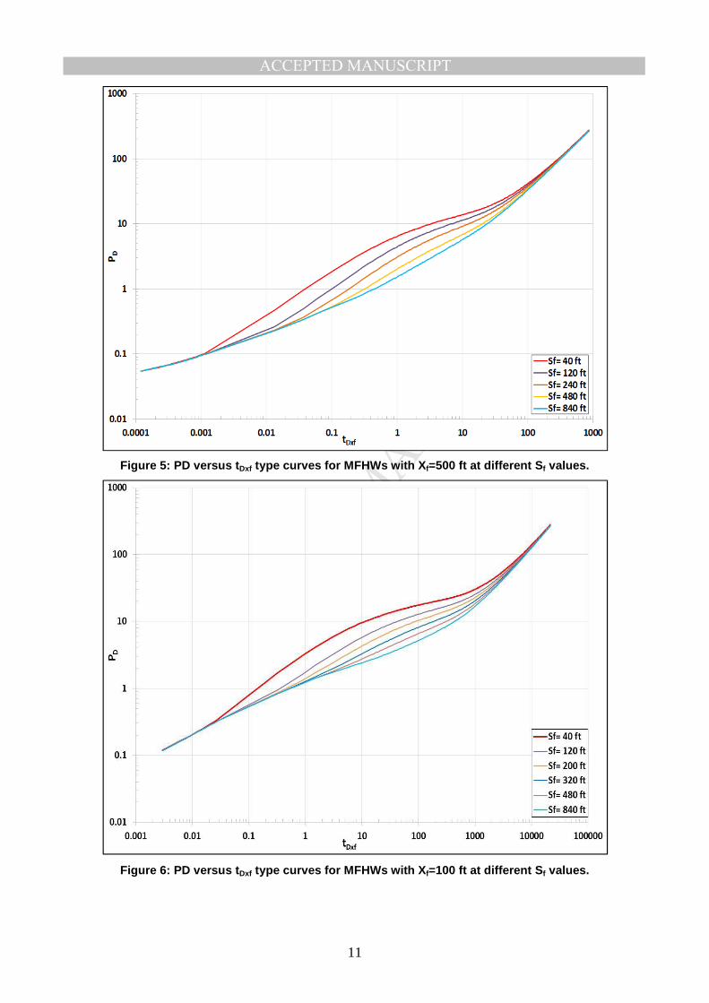
As mentioned before, for many cases, the compound linear flow regime was observed. To

further highlight the importance of this flow regime, the results of some of the simulations

described above have been used to generate sets of dimensionless pressure (PD) versus

dimensionless time (tDxf) type curves, which are shown in Figures 4-6 for Xf=1020, 500 and

100 ft., respectively. These type curves were generated based on Equation 6 and Equation 7

for a range of fracture spacing of 40 to 840 ft.

MANUSCRIP

T

ACCEPTED

ACCEPTED MANUSCRIPT

10

�' � ��ℎ%�� � ���)141.2�� Equation 6

�':� � 0.00633���∅���"�� Equation 7

where PD is the dimensionless pressure, tDxf is the dimensionless time and Pwf is the flowing

bottom-hole pressure.

These Figures illustrate that the type curves for different values of Sf overlap each other at the

early time (linear) and late time (boundary dominated) flow conditions; highlighting that the

intermediate time between these two flow periods is important for characterising the systems.

Figure 4: PD versus tDxf type curves for MFHWs with Xf=1020 ft at different Sf values.

MANUSCRIP

T

ACCEPTED

ACCEPTED MANUSCRIPT

11

Figure 5: PD versus tDxf type curves for MFHWs with Xf=500 ft at different Sf values.

Figure 6: PD versus tDxf type curves for MFHWs with Xf=100 ft at different Sf values.

MANUSCRIP

T

ACCEPTED

ACCEPTED MANUSCRIPT

12

Thompson et al. (2012) used the definition of the compound linear flow regime by van

Kruysdijk (1989) and proposed an analytical solution for it. Van Kruysdijk identified this

flow regime “as the well response, as if, it drains a linear reservoir with a width equal to the

distance between the outer fractures”. Thompson et al. proposed that if Xf in Equation 8,

which was proposed by Wattenbarger et al. (1998) as a reduced, dimensionless form of

Equation 2 is replaced by the half-length of the well (L w/2), the solution for the compound

linear flow regime, Equation 9, could be expressed by: �' � 7<�':� Equation 8

�' � 2 "�=� 7<�':� Equation 9

In this formulation, it is assumed that the well is drilled through the entire length of the

drainage area i.e. Lw=2Xe, as shown in Figure 7. Thus, Equation 9 could not always be valid

because the well may not go through the whole reservoir and/or the contribution of the

reservoir beyond the stimulated area to the total production is significant.

Figure 7: A multi-fractured horizontal well drilled through the whole reservoir length.

Here, three different cases with various well lengths are discussed to demonstrate the

limitation of Equation 9 in tight reservoirs. Figure 8 compares the bottom-hole pressure of the

various cases obtained by the dimensionless equations suggested by Thompson et al. (2012)

with those obtained from reservoir simulations. The Figure shows that as the Lw/Xe ratio

decreases from 2 to 0.6, the accuracy of the prediction from the dimensionless equations

decreases drastically. Therefore, new equations are required, which have been developed as

described in the next section.

Ye

Lw = 2Xe

Xf

MANUSCRIP

T

ACCEPTED

ACCEPTED MANUSCRIPT

13

Figure 8: Comparison of the simulation results with the results obtained from the available

equations, Km=0.1 mD, Xf=500 ft for various Lw/Xe values of 2, 1.1 and 0.6.

3.2.1 New Definition of the Compound Linear Flow

To achieve the desired solution, a new and wider definition of the compound linear flow is

introduced in this study, where the exposed area to the flow is dynamic. In other words, the

area changes with time and is not limited to the cross-section of the well as assumed by

previous researchers. The area starts expanding from the stimulated area as soon as the

interference of fractures occurs while the flow behaviour is still linear, (half-slope in the

derivative on a log-log diagnostic plot). For example, Figure 9 (a, b and c), shows the

pressure profiles at different times (t=2, 7 and 10 years) of production, when a well with 7

fractures in the reservoir with Km=0.001 mD produced under compound linear flow. The

dominance of compound linear flow is confirmed using well testing analysis with

corresponding data shown in Figure 10. This Figure shows the derivative of pressure of this

flow regime is linear (slope=0.5) for a considerable amount of time; however, the area is not

limited to the well area.

Here, Equation 10 is proposed to calculate the dynamic area by considering the pressure

propagation beyond the stimulated volume over time.

MANUSCRIP

T

ACCEPTED

ACCEPTED MANUSCRIPT

14

� � �1 + �� + 2ℎ> ! ?948�ABC�DBC E� Equation 10

where A1 is the cross area of well (Lw*h) as shown in Figure 2, A2 is the side area of the well

(2Xfh), η is the formation diffusivity, tscl and tecl are the start and the end times of the

compound linear flow and t is the time elapsed from the end of the early linear flow (tel).

In the third term of the equation, the concept of radius of investigation has been used to

account for the additional dynamic area beyond the fractured area over time.

This definition of the exposed area allows using the general form of linear flow equation for

calculating pressure profile of the compound linear flow regime as follows:

��� � �� � �8.128�� � � ����∅��� Equation 11

where, qt is the total production rate of the well and A is calculated at any time by Equation

10. It should be noted that if the compound linear flow does not disappear after reaching the

first boundary, the 2Xeh should be used for A instead of the output of the Equation 10 as the

pressure has reached the reservoir boundaries.

MANUSCRIP

T

ACCEPTED

ACCEPTED MANUSCRIPT

15

Figure 9: A schematic of the compound linear flow propagating over time, Km=0.001 mD.

c) t= 10 years

b) t= 7 years

a) t= 2 years

MANUSCRIP

T

ACCEPTED

ACCEPTED MANUSCRIPT

16

Figure 10: The pressure and derivative of pressure profiles of the well, Nf=7, Sf=600 ft, Xf=500 ft

and Km=0.001 mD.

3.3 Transitional Flow Periods

As already mentioned, the transitional flow periods contribute to a large bulk of MFHW

production and hence, need to be considered in the production forecasting. The following

Lagrange polynomial approximation is proposed to capture the MFHW performance during

these periods properly: �' � FGH%I%�':�)) Equation 12

where:

IJ�':�K �-ln�'NO ln�' � ln �'Pln �'N � ln �'P�QPN Equation 13

To use Equation 12 and Equation 13, a number of data points from the solutions of the early

linear, compound linear and PSS are required to be used to find the best curve that fits the

data before the equation is used to interpolate the other points in the corresponding transition

zones. That is, if this equation is applied for the first transitional period (between the early

and the intermediate flow periods), tDk and tDj are a number of points in the early linear and

compound linear flow periods, respectively, with known solutions PDk.

Compound linear flow

MANUSCRIP

T

ACCEPTED

ACCEPTED MANUSCRIPT

17

For the second transitional period, tDk, tDj are a number of points in the intermediate and PSS

times with known solutions of PDk.

For a given number (k) of discrete points, there are many possible interpolating functions;

however, the Lagrange polynomial, first introduced by Waring (1779), finds the one unique

function with degree of (k-1). In addition, the durations of the transition periods are expected

to be long, which cause a large variation in known solutions of flow regimes before and after

the transition periods. In mathematics, these are called the functions with high condition

number. The Lagrange polynomial are recommend to solve such problems (Gautschi 1974).

It should be noted that when constructing the polynomials, there is a trade-off between a

better fit and a smooth well-behaved fitting function. The more data points that are used in

the interpolation, the higher the degree of the resulting polynomial, and therefore the greater

oscillation it will exhibit between the data points. Therefore, a high-degree interpolation may

be a poor predictor of the function between points; however, the accuracy at the data points

will be perfect.

3.4 Results and Discussion

Various MFHWs scenario, which were not used before, were simulated using the same

simulator to investigate the reliability of the new model for capturing the unsteady state

performance of MFHWs in the transient period. It has to be also added that the equations are

valid for cases that primarily meets the underlying assumptions.

Figure 11 shows the bottom-hole pressure profiles that have been obtained from various

modelling approaches for a MFHW with 7 fractures and the half-length of 500 ft at a spacing

of 600 ft in a reservoir with Km=0.001 mD. For this case, the well has produced under early

linear flow regime for 75 days without fractures interference followed by 10 years of

compound linear flow as shown in Figure 10. Compared with the numerical simulation

results, the Figure shows that the commonly used formulations (i.e. Thompson et al.’s

equations) significantly underestimates the bottom-hole pressures in the transient flow period.

However, using the concept of dynamic area has significantly improved the prediction of the

pressure profile.

Another MFHW design (with Nf=7, Xf=500 and Sf=320) and Km=0.1 mD was considered.

The bottom-hole pressure profile obtained from the new method for this case has been

compared with those obtained from numerical simulation and the commonly used equations

as shown in Figure 12. The Figure shows a considerable improvement in the predictions

MANUSCRIP

T

ACCEPTED

ACCEPTED MANUSCRIPT

18

when using the new approach has been used compared to those predicted by the Thompson’s

equation.

Figure 11: Comparison of bottom-hole pressure in transient period obtained from various

approaches (Km=0.001 mD, Nf= 7, Sf= 600 ft and Xf=500 ft).

Figure 12: Comparison of bottom-hole pressure in transient period obtained from various

approaches (Km=0.1 mD, Nf=7, Sf= 320 ft and Xf=500 ft).

MANUSCRIP

T

ACCEPTED

ACCEPTED MANUSCRIPT

19

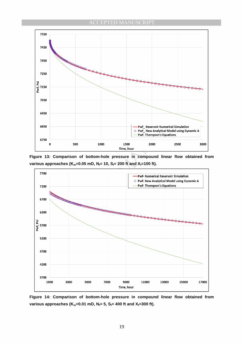
Figure 13: Comparison of bottom-hole pressure in compound linear flow obtained from

various approaches (Km=0.05 mD, Nf= 10, Sf= 200 ft and Xf=100 ft).

Figure 14: Comparison of bottom-hole pressure in compound linear flow obtained from

various approaches (Km=0.01 mD, Nf= 5, Sf= 400 ft and Xf=300 ft).

MANUSCRIP

T

ACCEPTED

ACCEPTED MANUSCRIPT

20

Figure 15: Comparison of the results from Lagrange polynomial approximation (red line) with

the reservoir simulation (blue dots) for the first transition period using the known solutions

(black dots).

Figure 13 and Figure 14 show the bottom-hole pressure profiles of other MFHWs examples

producing under compound linear flow regimes. Figure 13 shows the performance of a

MFHW design with Nf=10, Xf=100 ft, Sf=200 ft and Km=0.05 mD while Figure 14 shows the

bottom-hole pressure profiles of another case with Nf=5, Xf=300 ft, Sf=400 ft, Km=0.01 mD.

These data demonstrate that compared to results of the numerical simulation and commonly

used equations, the new equation has significantly improved the prediction of the pressure

profiles when using the dynamic area concept.

Figure 15 shows the application of the procedure proposed for predicting the transition

periods. In this Figure, a number of known points from the early linear and compound linear

flow regime solution have been used to estimate the performance of the first transition zone.

The Figure also confirms the good predictive capability of Equation 10, in terms of matching

the reservoir simulation outputs and when compared to the predictions of the Thompson’s

equation.

It should be noted if optimising the performance of well based on a short-term objective (i.e.

before the interference time) is aimed, these new equations could also be used for the targeted

time.

MANUSCRIP

T

ACCEPTED

ACCEPTED MANUSCRIPT

21

3.5 Well Lifetime Performance Prediction

Combining the developed transient time models with a model suitable for the boundary

dominated flow enable us to simulate the MFHWs lifetime performance. For this purpose,,

the PSS based PI equation developed for MFHWs in tight reservoirs by the authors

(MoradiDowlatabad and Jamiolahmady 2015) is used.

The time for the pressure to establish a boundary-dominated flow could be estimated by:

�RSS � 3790 ∅������ �'TRSS Equation 14

where tpss is the PSS time and tDApss is the shape factor value, which depends on the geometry

and well placement.

In addition, by writing the material balance for a slightly compressible single-phase fluid, the

average reservoir pressure at PSS time could be obtained by the following:

�U � �� � V1 � WXW Y% Z� Z )%1 + �U) Equation 15

where Pr is the average reservoir pressure at PSS time, N is the original fluid-in-place, NP is

the cumulative fluid production up to the PSS time and Boi and Bo are the fluid formation

volume factors at initial and PSS times, respectively.

After PSS time, the reservoir pressure at a specific time could be calculated by applying the

material balance and using the fact that the pressure gradient over time is constant for the

reservoir at pseudo steady state condition. Therefore, as: EHE� � �0.23396� ���ℎ∅ Equation 16

The average reservoir pressure could be calculated using the equation below:

�U,�\1 � �U,� � 0.23396� ∆����ℎ∅ Equation 17

where Pr,i+1 and Pr,i are the average reservoir pressures at time steps i and i+1 after PSS time

and ∆t is the time difference between the two time-steps. Using Equation 18, the well

performance can be obtained:

���,�\1 � �U,�\1 � �� �̂ Equation 18

where � _̂ is the MFHWs productivity index. Therefore, by combining Equation 17 and

Equation 18, the flowing bottom-hole pressure (Pwf) could be calculated by:

���,�\1 � `�U,� � 0.23396� ∆����ℎ∅ a � �� �̂ Equation 19

MANUSCRIP

T

ACCEPTED

ACCEPTED MANUSCRIPT

22

Various MFHWs scenarios were simulated to investigate the reliability of the new model for

capturing the full well-life performance of MFHWs.

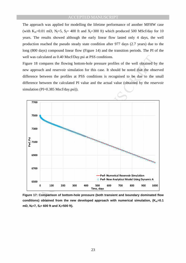
Figure 17 shows the bottom-hole pressure profiles that have been obtained from two

modelling approaches (numerical reservoir simulation and the new analytical solution) for a

MFHW (with Nf=7, Xf=500 and Sf=600 ft) in a reservoir with Km=0.1 mD that produces at a

constant rate of 500 MScf/Day for 1000 days. It is noted that for this case, the well produces

under unsteady state flow conditions for almost three months. The interference time for this

case is about 18 hours, while the well produces under the compound linear flow for 70 days.

Figure 16 shows that 8 data points from the compound linear flow and 10 points from the

boundary-dominated flow have been used to create the polynomials, which model the

performance of the second transitional period. Similar procedure has been followed for the

first transition period with points taken from the early linear and compound linear flow

regimes. PI has been calculated to be 6.92 MScf/Day.psi. Figure 17 shows a very close

agreement between pressure profiles from the new developed approach and numerical

simulation.

Figure 16: Comparison of the results from Lagrange polynomial approximation (black line)

with the reservoir simulation (Red dots) for the second transition period using the known

solutions (Blue dots).

MANUSCRIP

T

ACCEPTED

ACCEPTED MANUSCRIPT

23

The approach was applied for modelling the lifetime performance of another MFHW case

(with Km=0.01 mD, Nf=5, Sf= 400 ft and Xf=300 ft) which produced 500 MScf/day for 10

years. The results showed although the early linear flow lasted only 4 days, the well

production reached the pseudo steady state condition after 977 days (2.7 years) due to the

long (800 days) compound linear flow (Figure 14) and the transition periods. The PI of the

well was calculated as 0.40 Mscf/Day.psi at PSS conditions.

Figure 18 compares the flowing bottom-hole pressure profiles of the well obtained by the

new approach and reservoir simulation for this case. It should be noted that the observed

difference between the profiles at PSS conditions is recognised to be due to the small

difference between the calculated PI value and the actual value (obtained by the reservoir

simulation (PI=0.385 Mscf/day.psi)).

Figure 17: Comparison of bottom-hole pressure (both transient and boundary dominated flow

conditions) obtained from the new developed approach with numerical simulation, (Km=0.1

mD, Nf=7, Sf= 600 ft and Xf=500 ft).

MANUSCRIP

T

ACCEPTED

ACCEPTED MANUSCRIPT

24

Figure 18: Comparison of flowing bottom-hole pressure (both transient and boundary

dominated flow conditions) obtained from the new developed approach with numerical

simulation, (Km=0.01 mD, Nf=5, Sf= 400 ft and Xf=300 ft).

3.6 Summary and Conclusions

In this study, the key features of transient flow around MFHWs in tight reservoirs were

studied.

1. It was demonstrated that although development of flow regimes around MFHWs

depend on the fracture geometry and reservoir properties, the early linear, compound

linear and boundary-dominated flow regimes are expected to be observed in most of

the practical cases.

2. The presented dimensionless type-curves illustrated the importance of the flow

behaviour in the intermediate time, mostly dominated by the compound linear, for

characterising the systems, as the early time linear flow and pseudo-steady-state parts

overlapped at many different prevailing conditions.

3. The analyses showed that the common formulation of linear flow is not applicable in

tight reservoirs where the well may not go through the whole reservoir and/or the

contribution of the reservoir beyond the stimulated area to the total production is

significant.

MANUSCRIP

T

ACCEPTED

ACCEPTED MANUSCRIPT

25

4. A new, general definition of the compound linear flow regime was introduced and

used to describe the flow during the compound linear flow period. The proposed

definition considers the exposed area to the flow to be dynamic (Equation 10) such

that the area changes with time.

5. A new approach based on the Lagrange polynomials, was also proposed to model the

two long transition periods between the three main flow regimes.

6. Combining these and the previously developed PI formulation, a simple, analytical

and practical model for forecasting the full lifetime performance of MFHWs was

proposed.

7. This analytical models can be used for tasks such as well testing, production

performance analyses, forecasting and optimisation of MFHWs design.

Acknowledgments

The above study was conducted as a part of the Unconventional Gas and Gas-condensate

Recovery Project at Heriot-Watt University. This research project is sponsored by: Daikin,

Dong Energy, Ecopetrol/Equion, ExxonMobil, GDF, INPEX, JX-Nippon, Petrobras, DEA,

Saudi-Aramco and TOTAL, whose contributions are gratefully acknowledged. The authors

also thank Schlumberger Information Solutions, Nutonian and MathWorks for access to their

software.

Nomenclature:

B Formation volume factor �� Initial Reservoir pressure

h Formation thickness �bU Reservoir pressure

HWs Horizontal wells Qg Gas production rate

Km Matrix permeability re Drainage radius

Kf Fracture permeability rw Wellbore radius

LGR Local grid refinement Sc Convergence skin

Km Matrix permeability Sf Fracture spacing

MFHWs Multiple fractured horizontal wells Wf Fracture width

N Original fluid-in-place Xe Drainage half-length in X

direction

MANUSCRIP

T

ACCEPTED

ACCEPTED MANUSCRIPT

26

PI Productivity index Ye Drainage half-length in Y

direction

Pwf Flowing Bottom-hole pressure µ Viscosity of the fluid

References

1. Al Ahmadi, H. A., Almarzooq, A. M. and Wattenbarger, R. A. (2010) 'Application of

Linear Flow Analysis to Shale Gas Wells - Field Cases', in SPE Unconventional Gas

Conference, Pittsburgh, Pennsylvania, USA, 2010/1/1/, SPE: Society of Petroleum

Engineers.

2. Arevalo-Villagran, J. A., Wattenbarger, R. A., Samaniego-Verduzco, F. and Pham, T.

T. (2001) 'Some History Cases of Long-Term Linear Flow in Tight Gas Wells', in

Canadian International Petroleum Conference, Calgary, Alberta, 2001/1/1/,

PETSOC: Petroleum Society of Canada.

3. Azari, M., Wooden, W. O. and Coble, L. E. (1990) 'A Complete Set of Laplace

Transforms for Finite-Conductivity Vertical Fractures Under Bilinear and Trilinear

Flows', in 1990/1/1/, SPE: Society of Petroleum Engineers.

4. Clarkson, C. R. (2013) 'Production data analysis of unconventional gas wells: Review

of theory and best practices', International Journal of Coal Geology, 109–110, 101-

146.

5. Gautschi, W. (1974) 'Norm estimates for inverses of Vandermonde matrices',

Numerische Mathematik, 23(4), 337-347.

6. Gringarten, A. C. and Ramey, H. J., Jr. (1973) 'The Use of Source and Green's

Functions in Solving Unsteady-Flow Problems in Reservoirs', SPE Journal Paper,

13(05), 285 - 296.

7. Ilk, D., Rushing, J. A., Perego, A. D. and Blasingame, T. A. (2008) 'Exponential vs.

Hyperbolic Decline in Tight Gas Sands: Understanding the Origin and Implications

for Reserve Estimates Using Arps' Decline Curves', in SPE Annual Technical

Conference and Exhibition, Denver, Colorado, USA, 2008/1/1/, SPE: Society of

Petroleum Engineers.

8. Lee, S.-T. and Brockenbrough, J. R. (1986) 'A New Approximate Analytic Solution

for Finite-Conductivity Vertical Fractures', SPE Formation Evaluation, 1(1), 75-88.

9. Lee, W. J. and Holditch, S. A. (1981) 'Fracture Evaluation With Pressure Transient

Testing in Low-Permeability Gas Reservoirs', Journal of Petroleum Technology,

33(09), 1776 - 1792.

MANUSCRIP

T

ACCEPTED

ACCEPTED MANUSCRIPT

27

10. Meyer, B. R., Bazan, L. W., Jacot, R. H. and Lattibeaudiere, M. G. (2010)

'Optimization of Multiple Transverse Hydraulic Fractures in Horizontal Wellbores', in

SPE Unconventional Gas Conference, Pittsburgh, Pennsylvania, 2010/1/1/, SPE:

Society of Petroleum Engineers.

11. Meyer, B. R. and Jacot, R. H. (2005) 'Pseudosteady-State Analysis of Finite

Conductivity Vertical Fractures', in SPE Annual Technical Conference and

Exhibition, Dallas, Texas, 2005/10/9, SPE: Society of Petroleum Engineers.

12. MoradiDowlatabad, M. and Jamiolahmady, M. (2015) 'Novel Approach for Predicting

Multiple Fractured Horizontal Wells Performance in Tight Reservoirs', in SPE

Offshore Europe Conference and Exhibition, Aberdeen, UK, 2015/9/8/, SPE: Society

of Petroleum Engineers.

13. Nobakht, M., Mattar, L., Moghadam, S. and Anderson, D. M. (2010) 'Simplified Yet

Rigorous Forecasting of Tight/Shale Gas Production in Linear Flow', in SPE Western

Regional Meeting, Anaheim, California, USA, 2010/1/1/, SPE: Society of Petroleum

Engineers.

14. Raghavan, R. S., Chen, C.-C. and Agarwal, B. (1997) 'An Analysis of Horizontal

Wells Intercepted by Multiple Fractures', SPE Journal, 02(03).

15. Thompson, J. M., Liang, P. and Mattar, L. (2012) 'What Is Positive About Negative

Intercepts', in SPE Canadian Unconventional Resources Conference, Calgary,

Alberta, Canada, 2012/1/1/, SPE: Society of Petroleum Engineers.

16. Valko, P. P. and Lee, W. J. (2010) 'A Better Way To Forecast Production From

Unconventional Gas Wells', in SPE Annual Technical Conference and Exhibition,

Florence, Italy, 2010/1/1/, SPE: Society of Petroleum Engineers.

17. van Kruysdijk, C. P. J. W., Dullaert, G. M. (1989) 'Boundary Element Solution of the

Transient Pressure Response of Multiply Fractured Horizontal Wells', in ECMOR I -

1st European Conference on the Mathematics of Oil Recovery, Cambridge, England,

01 July 1989, EAGE.

18. Wattenbarger, R. A., El-Banbi, A. H., Villegas, M. E. and Maggard, J. B. (1998)

'Production Analysis of Linear Flow Into Fractured Tight Gas Wells', in SPE Rocky

Mountain Regional/Low-Permeability Reservoirs Symposium, Denver, Colorado,

1998/1/1/, SPE: Society of Petroleum Engineers.

MANUSCRIP

T

ACCEPTED

ACCEPTED MANUSCRIPT

28

MANUSCRIP

T

ACCEPTED

ACCEPTED MANUSCRIPT

In this study, the key features of transient flow around MFHWs in tight reservoirs are studied.

1. It is demonstrated that although development of flow regimes around MFHWs depend

on the fracture geometry and reservoir properties, the early linear, compound linear

and boundary-dominated flow regimes are expected to be observed in most of the

practical cases.

2. The presented dimensionless type-curves illustrate the importance of the flow

behaviour in the intermediate time, mostly dominated by the compound linear, for

characterising the systems, as the early time linear flow and pseudo-steady-state parts

overlapped at many different prevailing conditions.

3. The analyses show that the common formulation of linear flow is not applicable in

tight reservoirs where the well may not go through the whole reservoir and/or the

contribution of the reservoir beyond the stimulated area to the total production is

significant.

4. A new, general definition of the compound linear flow regime is introduced and used

to describe the flow during the compound linear flow period. The proposed definition

considers the exposed area to the flow to be dynamic such that the area changes with

time.

5. A new approach based on the Lagrange polynomials, is also proposed to model the

two long transition periods between the three main flow regimes.

6. Combining these and the previously developed PI formulation, a simple, analytical

and practical model for forecasting the full lifetime performance of MFHWs was

proposed.

7. This analytical models can be used for tasks such as well testing, production

performance analyses, forecasting and optimisation of MFHWs design.