THE LEGISLATIVE,

ECONOMIC, AND ETHICAL

EFFECTS OF BIOFUEL

MANDATES The Unintended Consequences

ABSTRACT This Paper reexamines biofuel

mandates in the United States of

America and Brazil, and expands upon

the unintended consequences. We

analyze the quantitative impacts of

biofuel production on agricultural

production, the relative energy

efficiency of biofuel, the impacts of

biofuel mandates on land usage and

international trade, and the

Renewable Identification Numbers

program set forth by the EPA

Renewable Fuel Standard. We

determine that the unintended

consequences of biofuel mandates far

outweigh their benefits.

Michael Millman (Economics and Computer Science), Kyle Zheng (Economics), Kyle Nitiss (Economics) Prepared for Professors R. Stephen Berry and George S. Tolley

Introduction

The Energy Policy Act was signed into law by President George W. Bush on July 29,

2005. The Act was meant to usher in much-needed changed in the energy industry, combatting

growing problems and effectively altering U.S. energy policy by introducing a new set of

standards, tax incentives, and loan guarantees. Within the Energy Policy Act of 2005 was the

Renewable Fuel Standard (RFS)—the first mandate of its kind—requiring transportation fuel in

the United States to contain a minimum volume of renewable fuels. The main motivation of this

Paper is the RFS, as the policies that it sets are what require the production and use of biofuels in

the United States.

The benefits of the Renewable Fuel Standard are clear. The mandate continues to be a

large contributor to American energy independence, as it is in effect, increasing the volume of

fuel available to consumers. Additionally, the mandate has brought the United States to the

forefront of ethanol production, of which it is now the world’s largest exporter. The world

continues to ask for greener alternatives to the consumption of fossil fuels, and through the

Renewable Fuel Standard, the United States was able to provide an answer—billions of dollars

in subsidies and research in biofuel production. The Expanded Renewable Fuel Standard requires

that 36 billion gallons of renewable fuels be blended by 20221.

However, many question the true motives of the RFS. Many of the policies instituted as a

result of the Renewable Fuel Standard can be described as purely political—agricultural special

interest groups benefited immensely from the passage of the bill, as products such as corn,

soybean, and sugar cane were suddenly in much higher demand in order to satisfy volume

1 Schnepf and Yacobucci. RFS: Overview and Issues, 1.

requirements. These special interest groups rest predominately within the heartland of the United

States, and serve as important constituents of the Republican Party.

Apart from the political motives of the RFS, the costs of such a mandate have largely

gone unchecked. The immense Washington lobbying presence of the biofuels market, and the

fact that the program is government-sponsored, have cut down on negative feedback. In

reviewing the literature, we only came across two substantive papers that argue our claim—that

biofuel mandates cost more for society than their benefits. In October of 2010, Randy Schnepf

and Brent Yacobucci of the Congressional Research Service published Renewable Fuel Standard

(RFS): Overview and Issues. The paper highlighted the effects and progress of the initiative over

the first five years of its deployment, and proceeded to discuss potential sustainability issues with

it moving forward. The paper discussed supply issues of corn ethanol, as well as a the more low-

level infrastructural and distributional issues associated with ethanol. Schnepf and Yacobucci

concluded that, although increased biofuel production can achieve energy security and

environmental goals, this may come at the cost of the objectives of other policy initiatives. More

concretely, they specifically mentioned “rapid expansion of biofuels production may have

unintended and undesirable consequences for agricultural commodity costs, fossil energy use,

and environmental degradation.”2

Also in 2010, Harry de Gorter and David R. Just published The Social Costs and Benefits

of Biofuels3, which analyzed the efficacy of alternative biofuel policies using a cost-benefit

analysis. In this paper, they determine that ethanol policies increase the inefficiency of farm

subsidies, effectively creating a zero-sum game in the agricultural industry. Furthermore, they

2 Ibid., 29 3 de Gorter and Just. Social Costs and Benefits of Biofuels, 1.

argue that sustainability standards are ineffective and should be re-designed. In their research,

they cite several older papers that argue ethanol policies fail such a cost-benefit analysis (Taylor

and Van Doren 2007, Metcalf 2008, Hahn and Cecot 2009). They also cite the 2008 Searchinger

et al. paper, which argues that ethanol policies actually create higher greenhouse gas emission

due to indirect land use changes.4

In this Paper, we argue that some of the previous literature may be incorrect, particularly

pertaining to biofuel mandates’ effects on the prices of agricultural products. However, it is

important to note that none of the previous research highlights in aggregate, the many facets of

negative externalities caused by biofuel mandates such as the Renewable Fuel Standard. We seek

to develop an argument based off the quantitative and qualitative impacts of biofuel production

on agricultural prices, the relative energy efficiency of biofuel, the impacts of mandates on

unintentional land use changes and international trade, and a deep examination of the Renewable

Identification Numbers trading system, and conclude that the costs of biofuel mandates are far

greater than their intended benefits.

Impact of Biofuels on Agricultural Prices

Biofuel mandates, particularly in the United States, were created in order to subsidize the

farming communities that produce the agricultural input necessary for production. The extent to

4 This is also a subject of this Paper.

which this relationship holds in practice has been the subject of many papers, employing

econometric time-series analysis to test this hypothesis. In 2012, the American Journal of

Agricultural Economics published The Impact of Biofuels on Commodity Food Prices:

Assessment of Findings. In this paper, Zilberman et al. compile and analyze the previous

literature that has investigated the relationship between biofuel prices and agricultural prices.5

Serra et al. (2011) used auto-regression to identify the relationships between ethanol, corn, and

gasoline prices from 1990-2008, finding a significant positive correlation between these data. A

similar—but multivariate—auto-regression analysis was performed by Zhang et al. (2009), who

found that changes in ethanol prices have short-term effects on agricultural commodity prices. In

all cases, a positive relationship was discovered between ethanol prices and corn prices.

However, the previous research largely concerns itself with price action, and not

necessarily with the fundamental drivers of the prices themselves. Instead of analyzing the

effects of ethanol prices on agricultural prices, we will consider the effects of ethanol production

on agricultural prices. In this portion of the paper, we will focus on the relationship between corn

and ethanol, as ethanol is the most prevalent form of biofuel in the United States; its primary

feedstock is corn. As we are only analyzing the effects of biofuel mandates on corn, it is not

appropriate to include the prices—or production—of gasoline and other blendstocks. The data

for this analysis spans June 2010 to November 2015, and comes from Quandl—an open source

financial database—and the Department of Energy (DOE) weekly petroleum status reports.

The granularity of the data immediately poses a problem for time-series analysis. Cash6

corn prices—as reported by Quandl—are settled daily, whereas ethanol production figures from

5 Hochman et al. Impact of Biofuels on Commodity Food Prices, 3. 6 Cash here refers to the spot price of corn, as opposed to the basis diff, measured by the difference between spot and the front-month futures contract.

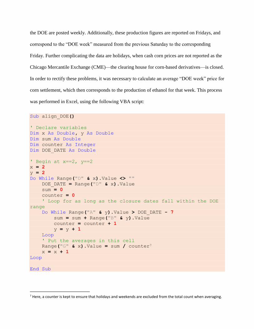
the DOE are posted weekly. Additionally, these production figures are reported on Fridays, and

correspond to the “DOE week” measured from the previous Saturday to the corresponding

Friday. Further complicating the data are holidays, when cash corn prices are not reported as the

Chicago Mercantile Exchange (CME)—the clearing house for corn-based derivatives—is closed.

In order to rectify these problems, it was necessary to calculate an average “DOE week” price for

corn settlement, which then corresponds to the production of ethanol for that week. This process

was performed in Excel, using the following VBA script:

Sub align_DOE()

' Declare variables

Dim x As Double, y As Double

Dim sum As Double

Dim counter As Integer

Dim DOE_DATE As Double

' Begin at x==2, y==2

x = 2

y = 2

Do While Range("D" & x).Value <> ""

DOE_DATE = Range("D" & x).Value

sum = 0

counter = 0

' Loop for as long as the closure dates fall within the DOE

range

Do While Range("A" & y).Value > DOE_DATE - 7

sum = sum + Range("B" & y).Value

counter = counter + 1

y = y + 1

Loop

' Put the averages in this cell

Range("G" & x).Value = sum / counter7

x = x + 1

Loop

End Sub

7 Here, a counter is kept to ensure that holidays and weekends are excluded from the total count when averaging.

After running the VBA script above, we have two vectors �⃑� and �⃑⃑�, where X represents

the weekly ethanol production figures reported by the DOE, and Y represents the average weekly

price of cash corn with respect to the DOE week. We graph the properly-aligned series in Figure

1 below:

Figure 1: This represents the ethanol production and cash corn price figures, properly aligned

and cleaned using VBA.

From the graph, it is not immediately apparent that the two variables exhibit any type of

relationship. However, there is clearly a period of interest in the data—between the middle of

2012 and the middle of 2013—when corn prices and ethanol production diverged significantly.

Moreover, the divergence occurs simultaneously. In the span of about one month, cash corn

prices rise approximately 47.8%, whereas ethanol production in the same period of time falls

approximately 13%. In order to identify possible causes for this phenomena, we researched

potential events in mid-2012 that could have resulted in such an event.

Research reveals that the summer of 2012 produced some of the most severe drought

conditions across the Midwestern United States in decades. Severe drought in corn-producing

0

1

2

3

4

5

6

7

8

9

700

750

800

850

900

950

1000

1050

20

11

20

12

20

13

20

14

20

15

Pri

ce o

f C

orn

($

10

0/b

ush

el)

Eth

ano

l Pro

du

ctio

n (

kbd

)

Year

Ethanol Production and Corn Prices

EthanolProduction

regions significantly lowered corn crop yields. As a result, corn futures prices increased 35%8

from June 18th to August 29th, and implied volatility of corn front-month options increased 14.3

percentage points, indicative of a large presence of speculative trading. Increased capital and

higher prices in the corn markets have tremendous effects on the price of ethanol, as

demonstrated in the Zhang and Serra papers. The largest feedstock of ethanol in the United

States is corn, and the American biofuel markets did not have the capacity to substitute

production with sugarcane or soybean. As a result, it is fair to hypothesize that ethanol prices

would also increase, but in this case, this price increase was not enough to counteract the lost

profits due to increased corn prices.

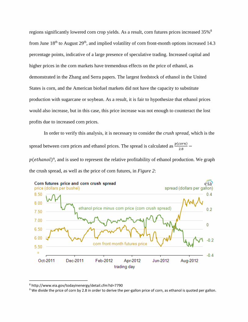
In order to verify this analysis, it is necessary to consider the crush spread, which is the

spread between corn prices and ethanol prices. The spread is calculated as 𝑝(𝑐𝑜𝑟𝑛)

2.8−

𝑝(𝑒𝑡ℎ𝑎𝑛𝑜𝑙)9, and is used to represent the relative profitability of ethanol production. We graph

the crush spread, as well as the price of corn futures, in Figure 2:

8 http://www.eia.gov/todayinenergy/detail.cfm?id=7790 9 We divide the price of corn by 2.8 in order to derive the per-gallon price of corn, as ethanol is quoted per gallon.

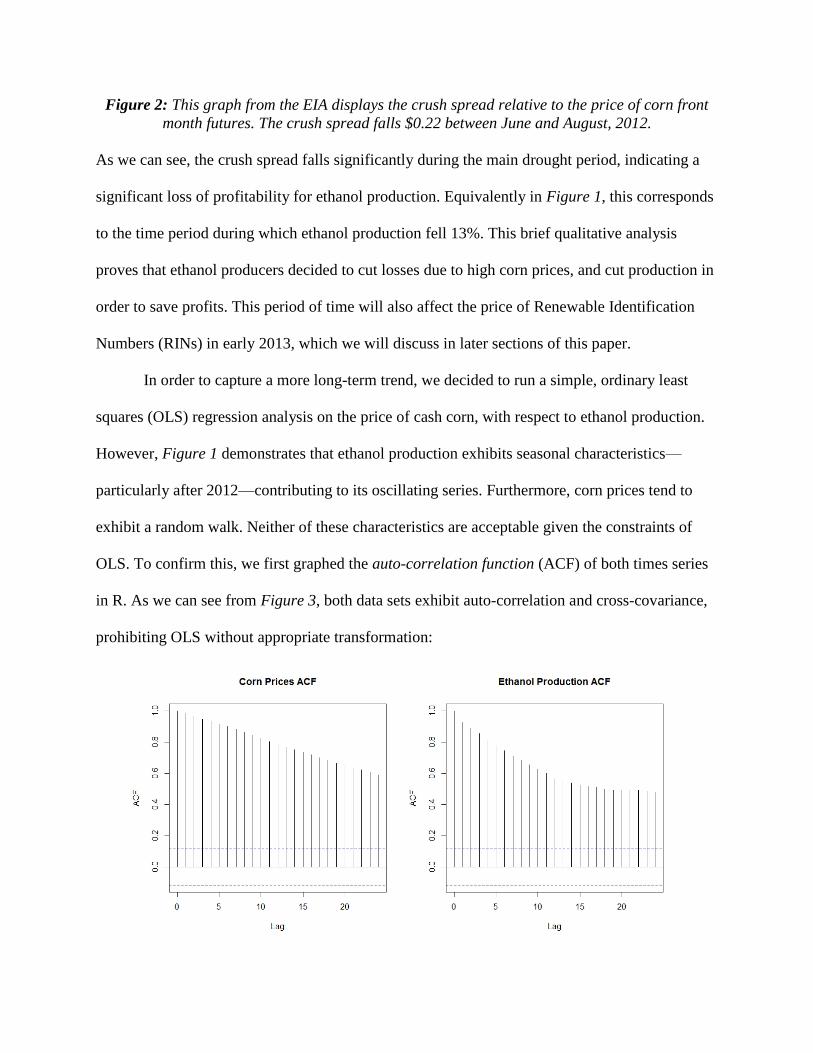
Figure 2: This graph from the EIA displays the crush spread relative to the price of corn front

month futures. The crush spread falls $0.22 between June and August, 2012.

As we can see, the crush spread falls significantly during the main drought period, indicating a

significant loss of profitability for ethanol production. Equivalently in Figure 1, this corresponds

to the time period during which ethanol production fell 13%. This brief qualitative analysis

proves that ethanol producers decided to cut losses due to high corn prices, and cut production in

order to save profits. This period of time will also affect the price of Renewable Identification

Numbers (RINs) in early 2013, which we will discuss in later sections of this paper.

In order to capture a more long-term trend, we decided to run a simple, ordinary least

squares (OLS) regression analysis on the price of cash corn, with respect to ethanol production.

However, Figure 1 demonstrates that ethanol production exhibits seasonal characteristics—

particularly after 2012—contributing to its oscillating series. Furthermore, corn prices tend to

exhibit a random walk. Neither of these characteristics are acceptable given the constraints of

OLS. To confirm this, we first graphed the auto-correlation function (ACF) of both times series

in R. As we can see from Figure 3, both data sets exhibit auto-correlation and cross-covariance,

prohibiting OLS without appropriate transformation:

Figure 3: The ACF plots above confirm significant auto-correlation.

To confirm this quantitatively, we ran an Augmented Dickey-Fuller test (ADF) on both data

series using the R command adf.test(). The results below contain p-values > 0.05, indicating that

we cannot reject the null hypothesis—the time series are non-stationary.

> adf.test(prod)

Augmented Dickey-Fuller Test

data: prod

Dickey-Fuller = -2.5291, Lag order = 6, p-value = 0.3532

alternative hypothesis: stationary

> adf.test(prices)

Augmented Dickey-Fuller Test

data: prices

Dickey-Fuller = -2.9868, Lag order = 6, p-value = 0.1603

alternative hypothesis: stationary

In order to derive OLS estimators, we will need to transform the data appropriately. M.B.

Priestley discusses common methods of handling non-stationary data in his paper, Non-Linear

and Non-Stationary Time Series Analysis (1988). One very simple method we can apply to our

data is the method of differences, in which, for a series X of n observations, X = x0, x1, … xn, and

a corresponding difference series Y of n-1 observations, we have yt = xt+1 – xt. We apply this

method to both the cash corn prices and ethanol production figures, and obtain Figure 4:

We observe a slight lag at the beginning of the series, but this tapers off in the rest of the series,

indicating our data is now stationary. To confirm this, we again run an ADF test on the

differenced data series, and obtain p-values < 0.01.10

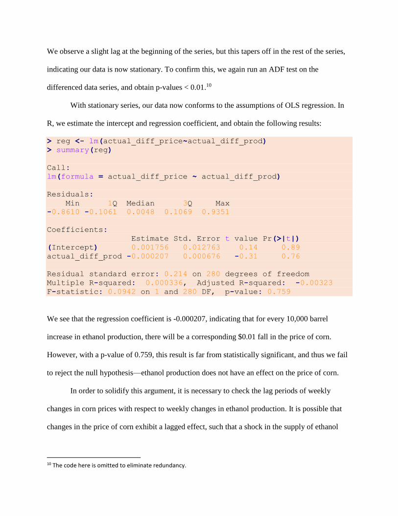
With stationary series, our data now conforms to the assumptions of OLS regression. In

R, we estimate the intercept and regression coefficient, and obtain the following results:

> reg <- lm(actual_diff_price~actual_diff_prod)

> summary(reg)

Call:

lm(formula = actual_diff_price ~ actual_diff_prod)

Residuals:

Min 1Q Median 3Q Max

-0.8610 -0.1061 0.0048 0.1069 0.9351

Coefficients:

Estimate Std. Error t value Pr(>|t|)

(Intercept) 0.001756 0.012763 0.14 0.89

actual_diff_prod -0.000207 0.000676 -0.31 0.76

Residual standard error: 0.214 on 280 degrees of freedom

Multiple R-squared: 0.000336, Adjusted R-squared: -0.00323

F-statistic: 0.0942 on 1 and 280 DF, p-value: 0.759

We see that the regression coefficient is -0.000207, indicating that for every 10,000 barrel

increase in ethanol production, there will be a corresponding $0.01 fall in the price of corn.

However, with a p-value of 0.759, this result is far from statistically significant, and thus we fail

to reject the null hypothesis—ethanol production does not have an effect on the price of corn.

In order to solidify this argument, it is necessary to check the lag periods of weekly

changes in corn prices with respect to weekly changes in ethanol production. It is possible that

changes in the price of corn exhibit a lagged effect, such that a shock in the supply of ethanol

10 The code here is omitted to eliminate redundancy.

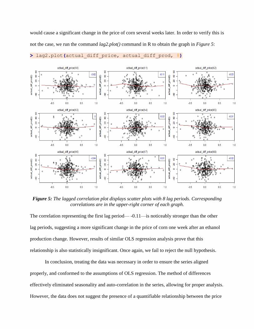
would cause a significant change in the price of corn several weeks later. In order to verify this is

not the case, we run the command lag2.plot() command in R to obtain the graph in Figure 5:

> lag2.plot(actual_diff_price, actual_diff_prod, 8)

Figure 5: The lagged correlation plot displays scatter plots with 8 lag periods. Corresponding

correlations are in the upper-right corner of each graph.

The correlation representing the first lag period— -0.11—is noticeably stronger than the other

lag periods, suggesting a more significant change in the price of corn one week after an ethanol

production change. However, results of similar OLS regression analysis prove that this

relationship is also statistically insignificant. Once again, we fail to reject the null hypothesis.

In conclusion, treating the data was necessary in order to ensure the series aligned

properly, and conformed to the assumptions of OLS regression. The method of differences

effectively eliminated seasonality and auto-correlation in the series, allowing for proper analysis.

However, the data does not suggest the presence of a quantifiable relationship between the price

of cash corn, and the ethanol production. Regardless of these results, a qualitative analysis of

corn prices and ethanol production yielded troubling information—the drastic fall in ethanol

production in 2012 and 2013 was primarily caused by a severe drought, driving up the price of

corn substantially. In this instance, biofuel production sustained marked impacts of a crisis

beyond control of the United States EPA mandates—drought. This study represents one

weakness of the U.S. biofuel mandate, and merits further consideration for policy changes.

Trends in Agricultural Production

Over the past fifteen years, ethanol production has boomed in the United States, tripling

between 2000 and 2007 and rising steadily thereafter. Between 2000 and 2014, ethanol

production grew from 1,622 million barrels to 14,340 million barrels, an increase of 884%.11 In

this section of the paper, the effect of this precipitous growth in ethanol production on U.S.

agriculture will be examined. In particular, as corn is the primary - and nearly exclusive -

feedstock for ethanol, we will examine the effect of rising ethanol production on the total yield

of production (in USD) of the top five U.S. cash crops (corn, soybeans, hay, wheat, and cotton).

In addition, we will also examine the energy inputs required for each of these cash crops in

service of determining whether the rise in ethanol production has affected the structure of crop

production, and consequently, whether a change in crop structure has significantly altered the

energy requirements for crop cultivation in the U.S.

In 2000, before the steep rise in ethanol production, corn comprised 28% of the total field

crop yield. Soybeans were the second leading crop at 19%, followed by hay, wheat, and cotton,

at 18%, 9%, and 6%, respectively.12 By 2014, corn’s share of the total field crop production had

11 Renewable Fuels Association. Industry Statistics. 12 USDA/NASS Database.

grown to 35%. Soybeans also increased in terms of share of total field crop yield to 27%, while

hay, wheat, and cotton fell to 13%, 8%, and 3% respectively.

Figure 1: Area chart of Top 5 U.S. Cash Crop Production

As illustrated in Figure 1, the increase in corn’s share of total field crop yield coincided

with the sharp increase in ethanol production. In 2011, corn’s share rose to 44%, accounting for

nearly half of total crop production in the U.S., and an increase in share of 12% from ten years

earlier. Another noteworthy trend illustrated in Figure 1 is that U.S. crop production as a whole

more than doubled between 2000 and 2014.

The total yield from corn rose between 2000 and 2014, growing faster than the rate at

which total field crop production grew and also faster than any other of the five major cash

crops. Given this growth, the next question the paper will concern itself with is what, if any,

discernible role did the rise in ethanol production have on the increase in corn production.

Figure 2: U.S. Use of Corn by Billions of Bushels13 Figure 3: U.S. Production of Corn($)

and Ethanol (mil. gallons)

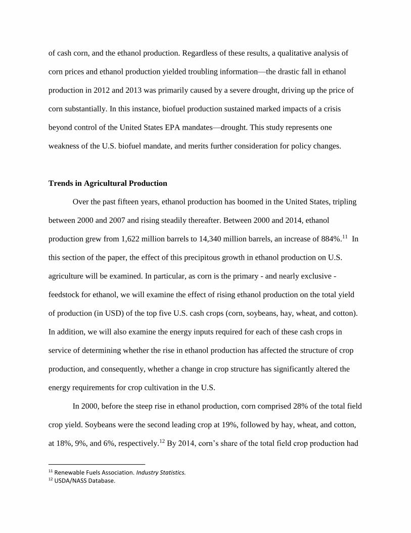
In Figure 2, it is evident that corn use for feed and export remained basically constant

over the period of observation, but corn use for ethanol rose dramatically. In 1990-1991, corn use

for ethanol was around half of what was used for export; by 2010-2011, more corn was being

used for ethanol production than was used for feedstock - a roughly fivefold increase in usage.

Clearly, growing ethanol production has played a role in the increasing production of corn. The

effect seems not to be as simple as ‘more ethanol = more corn’. The downside of using total

yield from production is that it encapsulates both the total amount of corn produced as well as

the price of corn. A more rigorous treatment of the relationship between corn prices and ethanol

production can be found elsewhere in the paper, but here we will take a slightly different

approach. To separate out the effect of corn prices on total yield of production from corn, we

examined the relationship between bushels of corn produced and ethanol production:

13 USDA, Economic Research Service. Feed Grains Database

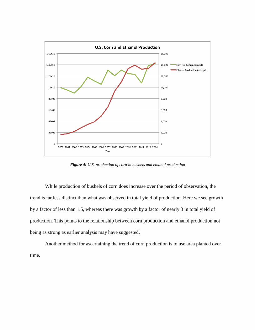
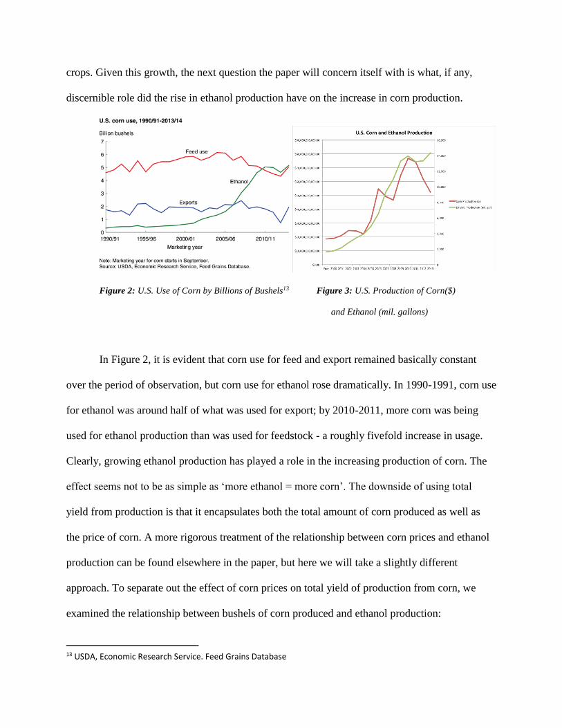
Figure 4: U.S. production of corn in bushels and ethanol production

While production of bushels of corn does increase over the period of observation, the

trend is far less distinct than what was observed in total yield of production. Here we see growth

by a factor of less than 1.5, whereas there was growth by a factor of nearly 3 in total yield of

production. This points to the relationship between corn production and ethanol production not

being as strong as earlier analysis may have suggested.

Another method for ascertaining the trend of corn production is to use area planted over

time.

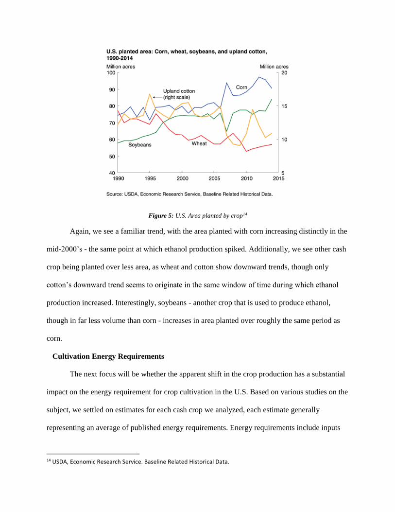
Figure 5: U.S. Area planted by crop14

Again, we see a familiar trend, with the area planted with corn increasing distinctly in the

mid-2000’s - the same point at which ethanol production spiked. Additionally, we see other cash

crop being planted over less area, as wheat and cotton show downward trends, though only

cotton’s downward trend seems to originate in the same window of time during which ethanol

production increased. Interestingly, soybeans - another crop that is used to produce ethanol,

though in far less volume than corn - increases in area planted over roughly the same period as

corn.

Cultivation Energy Requirements

The next focus will be whether the apparent shift in the crop production has a substantial

impact on the energy requirement for crop cultivation in the U.S. Based on various studies on the

subject, we settled on estimates for each cash crop we analyzed, each estimate generally

representing an average of published energy requirements. Energy requirements include inputs

14 USDA, Economic Research Service. Baseline Related Historical Data.

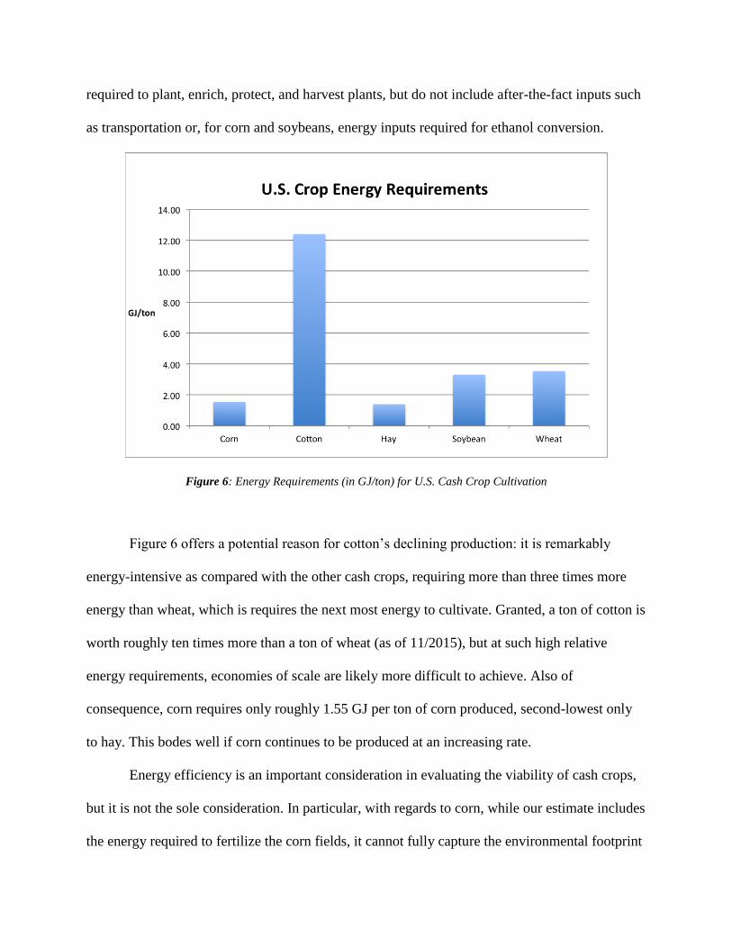
required to plant, enrich, protect, and harvest plants, but do not include after-the-fact inputs such

as transportation or, for corn and soybeans, energy inputs required for ethanol conversion.

Figure 6: Energy Requirements (in GJ/ton) for U.S. Cash Crop Cultivation

Figure 6 offers a potential reason for cotton’s declining production: it is remarkably

energy-intensive as compared with the other cash crops, requiring more than three times more

energy than wheat, which is requires the next most energy to cultivate. Granted, a ton of cotton is

worth roughly ten times more than a ton of wheat (as of 11/2015), but at such high relative

energy requirements, economies of scale are likely more difficult to achieve. Also of

consequence, corn requires only roughly 1.55 GJ per ton of corn produced, second-lowest only

to hay. This bodes well if corn continues to be produced at an increasing rate.

Energy efficiency is an important consideration in evaluating the viability of cash crops,

but it is not the sole consideration. In particular, with regards to corn, while our estimate includes

the energy required to fertilize the corn fields, it cannot fully capture the environmental footprint

these fertilizers leave. Corn, specifically, requires a large amount of nitrogen in the soil to

flourish - indeed it is the most nitrogen-intensive crop grown in the U.S. The immense amount of

nitrogen used in corn cultivation has several drawbacks, the most grave of which are nitrogen-

contaminated runoff water polluting rivers and oceans, and the release of nitrous oxides which

are potent greenhouse gases. These consequences will only grow worse as corn production - and

therefore nitrogen-fertilizer use increases - and will continue to do so unless containment of these

fertilizer byproducts improves dramatically.

Brazil as a Case Study

Brazil is the world’s second largest producer of ethanol, and produces most of its

ethanol from sugarcane. Its levels of ethanol production are exceeded only by the United States,

and together, the two nations produced 83% of the entire world’s ethanol in 2014. Figure 1,

taken from the Alternative Fuels Data Center (AFDC) shows the global production volume of

ethanol and the shares of production for each of the world’s major producers.

Figure 1: Global Ethanol Production by Volume and Share of Production15

15 DOE, Alternative Fuels Data Center. Maps and Data.

While Brazil is one of the largest economies in the world, there are reasons for its high share of

global ethanol production that explain why it produces so much more than countries with larger

economies, such as China and several countries in Europe.

To better understand these reasons, we will first examine the ethanol production process

in order to glean insights as to why Brazil is positioned so well to produce such large volumes of

ethanol. Because Brazil produces its ethanol from sugarcane, we will focus on this specific

production process. We will also examine the wider Brazilian economy to see why ethanol

production levels are so high, and investigate the history of energy policy in Brazil. In doing so,

we hope to learn the effects of biofuel and energy mandates on the Brazilian economy, to see

their benefits and consequences.

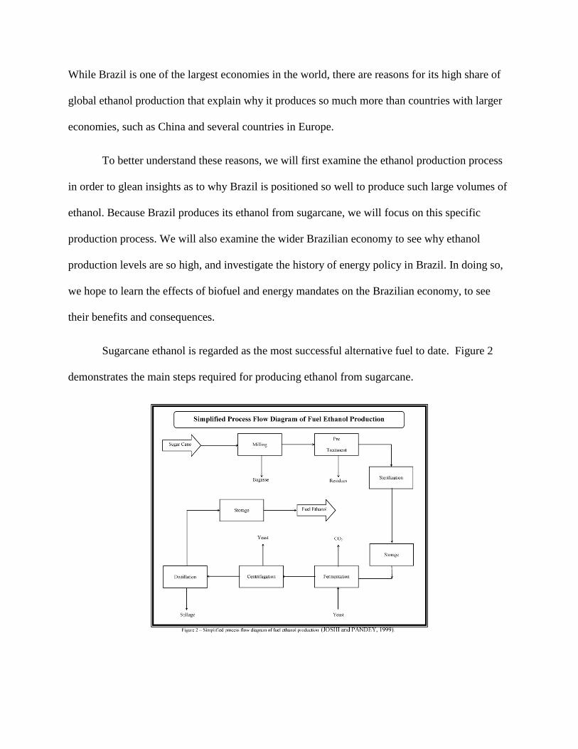
Sugarcane ethanol is regarded as the most successful alternative fuel to date. Figure 2

demonstrates the main steps required for producing ethanol from sugarcane.

Figure 2: A Simplification of the Production Process for Sugarcane Ethanol16

The end product from this process, fuel ethanol, is nearly identical to the ethanol produced when

other feedstock, such as corn or wheat. A major advantage that sugarcane has over other

feedstock is that it yields nine times more energy than it consumes during the process. This

energy balance is over four times better than ethanol produced from wheat or sugarbeet, and

nearly seven times that of corn ethanol. Brazilian sugarcane ethanol is also the most productive

feedstock, as it produces 7,500 liters of fuel per hectare, compared to the 5,500 liters per hectare

of European sugarbeet and 3,800 liters per hectare of U.S. corn.17

The advantages of using sugarcane as a feedstock for ethanol contribute to Brazil’s

ability to produce so much ethanol, but there are other reasons for its high levels of productions.

Figure 3: A Map of Brazil showing the Locations of Land Used for Sugarcane Farming18

16 SCI ELO, Proceedings. 17 SugarCane.org, Producing Food and Fuel. 18 Ibid., Preserving Biodiversity.

While its economy is not quite as strong as several countries in Europe and Asia, Brazil’s land

mass allows it to farm more feedstock than countries in Europe or Asia. Yet Brazil only

extensively utilizes two regions of its entire country for sugarcane farming. Figure 3 shows the

portion of Brazil that contributes to the ethanol production industry. In addition to the relatively

small amount of land required for sugarcane ethanol production, this process is also

environmentally friendly in the way that it does not impose on the rainforests in Brazil, which

are a major topic of concern for environmentalists.

We can also point to Brazil’s relatively strong economy that allows it to support the

infrastructure required to operate a large-scale ethanol industry. Relative to larger countries that

could feasibly farm as much as Brazil, such as other countries in South America, Brazil has a

more capable economy that allows it to farm and produce more than such countries. It has a GDP

of 2346.12 billion USD19, compared to the country with the second highest GDP in Latin

America, Argentina, which has a GDP of 540.20 billion USD. In addition to its relatively large

size and economy, biofuel mandates that emphasize sugarcane production are major reasons for

Brazil’s booming biofuel production.

In the 1930s, Brazil began to blend ethanol and gasoline to provide as a source of fuel.

By the 1970s, 80% of oil was imported, and 98% of public and industrial transportation relied on

oil and oil derivatives for energy.20 As a result, the country was drastically affected by the oil

crisis in the 1970, so the Brazilian government decided to adjust the country’s energy strategy to

increase the emphasis on biofuels, and subsequently increase its energy supply.21 There were

several incentives for the implementation of this program. At the pricing level, ethanol prices

19 Trading Economics. Brazil GDP. 20 Giacomazzi. A Brief History of Brazilian Proalcool Programe 21 Soccol et al. Brazilian Biofuel Program: An Overview, 5.

were lower than gasoline prices, and taxes are lower for vehicles moved by ethanol.

Additionally, the program would help producers by one, insuring that they would be paid for

their product, and two, through government aid in financing their production to increase

production capacities. The program would also allow the country to internally maintain its

strategic reserves so that it could respond to future shocks.

In 1975, the ProAlcool program was implemented, with the goal of slowing down energy

consumption by producing ethanol from biomasses, such as sugarcane, cassava, and sorghum, to

substitute for gasoline. In phase one of the program, anhydrous alcohol was mixed with gasoline

to have a mixture of up to 20% alcohol. To achieve this, the country embarked to increase

alcohol production from 600,000 liters/year to 3B liters/year. They accomplished this by

subsidizing the expansion of and investment in the sugarcane mills and distilleries. The

government viewed this energy strategy as more flexible and adaptive to changes in crop and

energy prices. If the price of sugarcane was low, then alcohol could be produced, and if the price

of alcohol was low, then sugarcane could be sold as a crop.

Phase two of the ProAlcool program began in 1980, as the government continued to

provide economic incentives for increasing the capacities and productivity of the sugarcane mills

and distilleries. Additionally, researchers began to use plants that were more productive for

producing alcohols, at the loss of the flexibility of being used to produce sugar. Figure 4 below

shows how ethanol production has increased over time since the start of the ProAlcoòl program.

Figure 4: Graph Depicting Production of Ethanol in Brazil since 197522

The ProAlcoòl program encouraged innovation in ethanol production processes, as it offered

financing for research and development of more efficient processes. As a result, Brazil was able

to increase the amount of sugarcane ethanol produced per hectare. Figure 5 demonstrates this

increase in productivity as a result of government financing and innovation of technology. As the

graph demonstrates, the yield of ethanol per hectare increased by 3.77% annually from 1975 to

2003, which is one of the major explanations for the increase in ethanol production in Brazil.

This also explains how the country can utilize so little of its land to produce so much ethanol.

On the consumption side, automobile factories were incentivized to produce cars that

could only use alcohol as a fuel. By 1984, 94% of passenger cars could only run on ethanol. The

country’s reliance on oil in the 1970s made them vulnerable to the oil crisis of that decade, just

as the country’s overreliance on ethanol would in the 1980s.

22 Azanha and Dias de Moraes. Reflections on Brazil’s Ethanol Industry, 139.

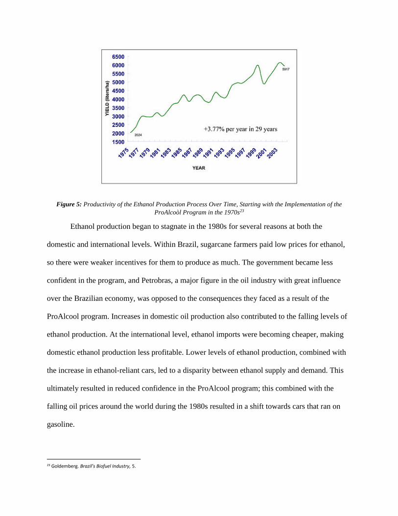
Figure 5: Productivity of the Ethanol Production Process Over Time, Starting with the Implementation of the

ProAlcoòl Program in the 1970s23

Ethanol production began to stagnate in the 1980s for several reasons at both the

domestic and international levels. Within Brazil, sugarcane farmers paid low prices for ethanol,

so there were weaker incentives for them to produce as much. The government became less

confident in the program, and Petrobras, a major figure in the oil industry with great influence

over the Brazilian economy, was opposed to the consequences they faced as a result of the

ProAlcool program. Increases in domestic oil production also contributed to the falling levels of

ethanol production. At the international level, ethanol imports were becoming cheaper, making

domestic ethanol production less profitable. Lower levels of ethanol production, combined with

the increase in ethanol-reliant cars, led to a disparity between ethanol supply and demand. This

ultimately resulted in reduced confidence in the ProAlcool program; this combined with the

falling oil prices around the world during the 1980s resulted in a shift towards cars that ran on

gasoline.

23 Goldemberg. Brazil’s Biofuel Industry, 5.

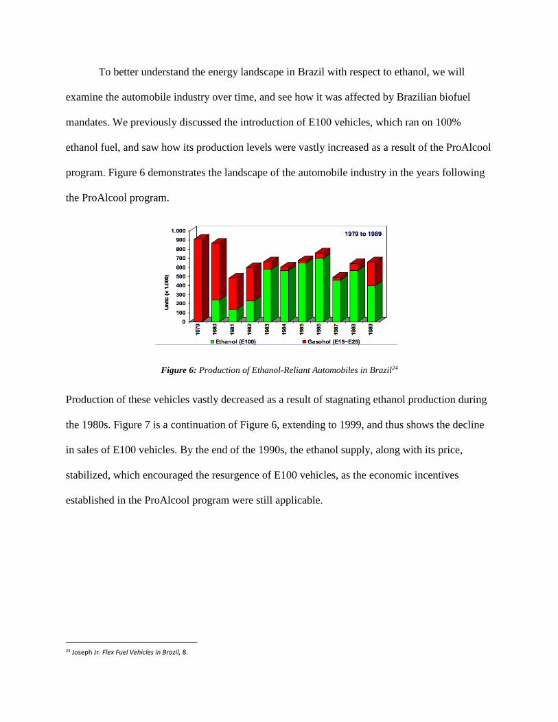
To better understand the energy landscape in Brazil with respect to ethanol, we will

examine the automobile industry over time, and see how it was affected by Brazilian biofuel

mandates. We previously discussed the introduction of E100 vehicles, which ran on 100%

ethanol fuel, and saw how its production levels were vastly increased as a result of the ProAlcool

program. Figure 6 demonstrates the landscape of the automobile industry in the years following

the ProAlcool program.

Figure 6: Production of Ethanol-Reliant Automobiles in Brazil24

Production of these vehicles vastly decreased as a result of stagnating ethanol production during

the 1980s. Figure 7 is a continuation of Figure 6, extending to 1999, and thus shows the decline

in sales of E100 vehicles. By the end of the 1990s, the ethanol supply, along with its price,

stabilized, which encouraged the resurgence of E100 vehicles, as the economic incentives

established in the ProAlcool program were still applicable.

24 Joseph Jr. Flex Fuel Vehicles in Brazil, 8.

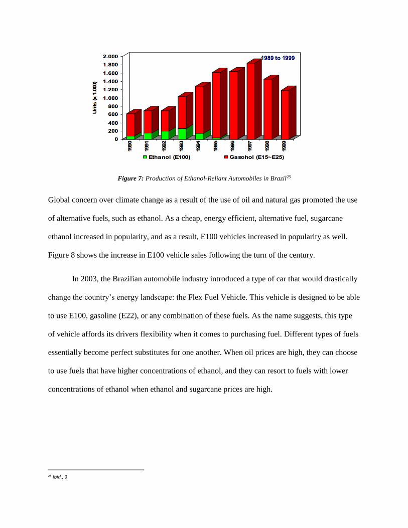
Figure 7: Production of Ethanol-Reliant Automobiles in Brazil25

Global concern over climate change as a result of the use of oil and natural gas promoted the use

of alternative fuels, such as ethanol. As a cheap, energy efficient, alternative fuel, sugarcane

ethanol increased in popularity, and as a result, E100 vehicles increased in popularity as well.

Figure 8 shows the increase in E100 vehicle sales following the turn of the century.

In 2003, the Brazilian automobile industry introduced a type of car that would drastically

change the country’s energy landscape: the Flex Fuel Vehicle. This vehicle is designed to be able

to use E100, gasoline (E22), or any combination of these fuels. As the name suggests, this type

of vehicle affords its drivers flexibility when it comes to purchasing fuel. Different types of fuels

essentially become perfect substitutes for one another. When oil prices are high, they can choose

to use fuels that have higher concentrations of ethanol, and they can resort to fuels with lower

concentrations of ethanol when ethanol and sugarcane prices are high.

25 Ibid., 9.

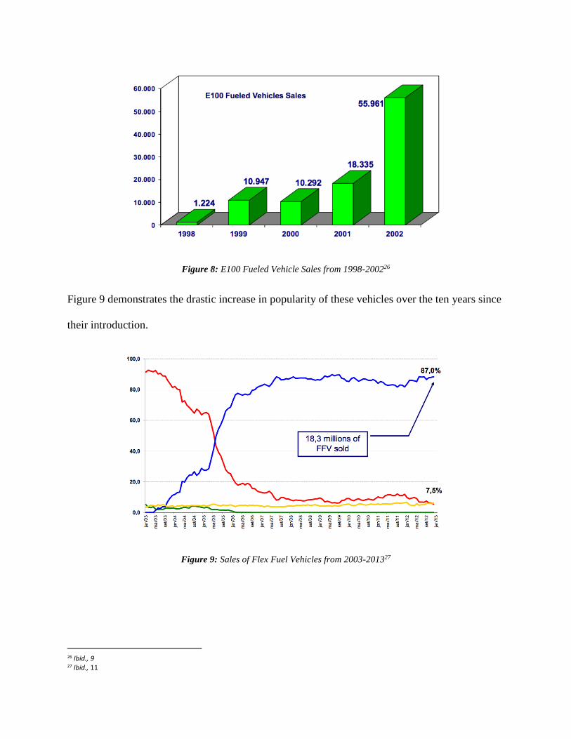
Figure 8: E100 Fueled Vehicle Sales from 1998-200226

Figure 9 demonstrates the drastic increase in popularity of these vehicles over the ten years since

their introduction.

Figure 9: Sales of Flex Fuel Vehicles from 2003-201327

26 Ibid., 9 27 Ibid., 11

In 2009, 92% of all new cars and light vehicles were equipped with flex-fuel technology. By

2011, flex-fuel vehicles made up 51% of all Otto cycle vehicles28, which include passenger cars,

light commercial vehicles, and motorcycles. 29

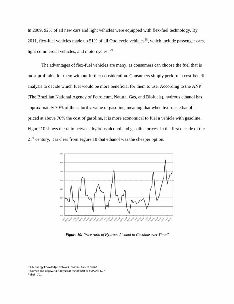
The advantages of flex-fuel vehicles are many, as consumers can choose the fuel that is

most profitable for them without further consideration. Consumers simply perform a cost-benefit

analysis to decide which fuel would be more beneficial for them to use. According to the ANP

(The Brazilian National Agency of Petroleum, Natural Gas, and Biofuels), hydrous ethanol has

approximately 70% of the calorific value of gasoline, meaning that when hydrous ethanol is

priced at above 70% the cost of gasoline, it is more economical to fuel a vehicle with gasoline.

Figure 10 shows the ratio between hydrous alcohol and gasoline prices. In the first decade of the

21st century, it is clear from Figure 10 that ethanol was the cheaper option.

Figure 10: Price ratio of Hydrous Alcohol to Gasoline over Time30

28 UN Energy Knowledge Network. Ethanol Fuel in Brazil 29 Gomez and Legey. An Analysis of the Impact of Biofuels, 697 30 Ibid., 701

This is consistent with our data above showing the increase in ethanol production in the period

leading up to, and during, the time series depicted in Figure 10, as increases in ethanol supply

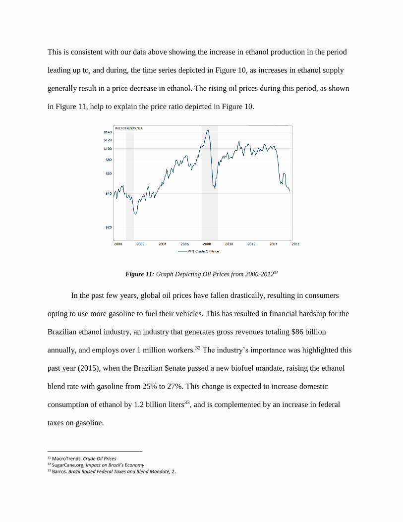
generally result in a price decrease in ethanol. The rising oil prices during this period, as shown

in Figure 11, help to explain the price ratio depicted in Figure 10.

Figure 11: Graph Depicting Oil Prices from 2000-201231

In the past few years, global oil prices have fallen drastically, resulting in consumers

opting to use more gasoline to fuel their vehicles. This has resulted in financial hardship for the

Brazilian ethanol industry, an industry that generates gross revenues totaling $86 billion

annually, and employs over 1 million workers.32 The industry’s importance was highlighted this

past year (2015), when the Brazilian Senate passed a new biofuel mandate, raising the ethanol

blend rate with gasoline from 25% to 27%. This change is expected to increase domestic

consumption of ethanol by 1.2 billion liters33, and is complemented by an increase in federal

taxes on gasoline.

31 MacroTrends. Crude Oil Prices 32 SugarCane.org, Impact on Brazil’s Economy 33 Barros. Brazil Raised Federal Taxes and Blend Mandate, 2.

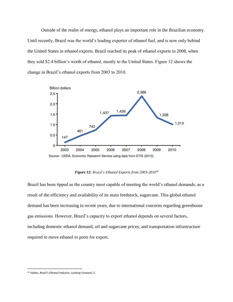
Outside of the realm of energy, ethanol plays an important role in the Brazilian economy.

Until recently, Brazil was the world’s leading exporter of ethanol fuel, and is now only behind

the United States in ethanol exports. Brazil reached its peak of ethanol exports in 2008, when

they sold $2.4 billion’s worth of ethanol, mostly to the United States. Figure 12 shows the

change in Brazil’s ethanol exports from 2003 to 2010.

Figure 12: Brazil’s Ethanol Exports from 2003-201034

Brazil has been tipped as the country most capable of meeting the world’s ethanol demands, as a

result of the efficiency and availability of its main feedstock, sugarcane. This global ethanol

demand has been increasing in recent years, due to international concerns regarding greenhouse

gas emissions. However, Brazil’s capacity to export ethanol depends on several factors,

including domestic ethanol demand, oil and sugarcane prices, and transportation infrastructure

required to move ethanol to ports for export.

34 Valdes. Brazil’s Ethanol Industry: Looking Forward, 3.

In recent years, mandates such as the one implemented in 2015 mentioned above, have

increased domestic consumption of ethanol, leaving less of a supply for the global market. Brazil

is the world’s second largest consumer of ethanol, behind the United States, and consumed 22.7

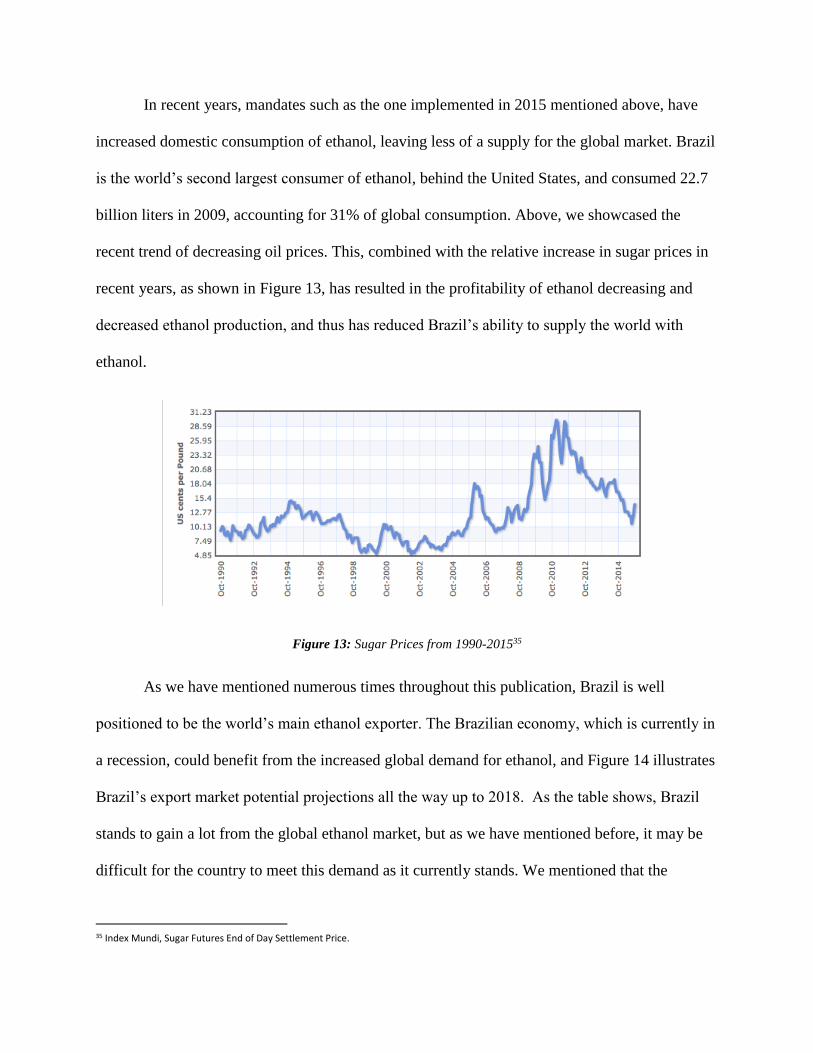
billion liters in 2009, accounting for 31% of global consumption. Above, we showcased the

recent trend of decreasing oil prices. This, combined with the relative increase in sugar prices in

recent years, as shown in Figure 13, has resulted in the profitability of ethanol decreasing and

decreased ethanol production, and thus has reduced Brazil’s ability to supply the world with

ethanol.

Figure 13: Sugar Prices from 1990-201535

As we have mentioned numerous times throughout this publication, Brazil is well

positioned to be the world’s main ethanol exporter. The Brazilian economy, which is currently in

a recession, could benefit from the increased global demand for ethanol, and Figure 14 illustrates

Brazil’s export market potential projections all the way up to 2018. As the table shows, Brazil

stands to gain a lot from the global ethanol market, but as we have mentioned before, it may be

difficult for the country to meet this demand as it currently stands. We mentioned that the

35 Index Mundi, Sugar Futures End of Day Settlement Price.

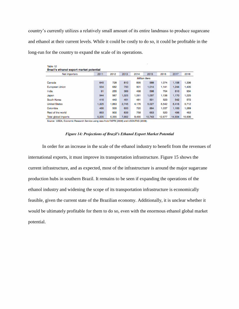
country’s currently utilizes a relatively small amount of its entire landmass to produce sugarcane

and ethanol at their current levels. While it could be costly to do so, it could be profitable in the

long-run for the country to expand the scale of its operations.

Figure 14: Projections of Brazil’s Ethanol Export Market Potential

In order for an increase in the scale of the ethanol industry to benefit from the revenues of

international exports, it must improve its transportation infrastructure. Figure 15 shows the

current infrastructure, and as expected, most of the infrastructure is around the major sugarcane

production hubs in southern Brazil. It remains to be seen if expanding the operations of the

ethanol industry and widening the scope of its transportation infrastructure is economically

feasible, given the current state of the Brazilian economy. Additionally, it is unclear whether it

would be ultimately profitable for them to do so, even with the enormous ethanol global market

potential.

Figure 15: Map of Brazil’s Ethanol Transportation Infrastructure36

However, given the fact that sugarcane is the world’s most efficient and successful biofuel

feedstock, and the fact that Brazil already boasts a strong infrastructure dedicated to its ethanol

industry, it is clear that Brazil is the world’s best option for meeting the rising demand for

ethanol.

Conversion of Corn into Ethanol: Energy Inputs

In this section of the paper, the process, as well as the energy requirements for converting

corn into ethanol fuel will be examined. The energy required to cultivate corn (in GJ/ton) was

discussed above, and the energy input required was found to be roughly 1.55 GJ/ton. This will

now be combined with estimates of the energy required to transport corn to ethanol fuel distilling

36 Valdes. Brazil’s Ethanol Industry: Looking Forward, 16.

sites, and to convert corn into ethanol. First, however, we will explain the process of distilling

ethanol from corn.

Distilling ethanol from corn involves one of two processes: dry-milling or wet-milling. In

either case, corn is mashed, allowed to ferment, and then distilled into ethanol. In the case of

wet-milling, corn is soaked in a solution which separates it into its component parts. Corn oil is a

byproduct of this process, and is bottled and sold. Additionally, the gluten proteins in the corn

can be extracted and turned into a nutritious feed for livestock. While these byproducts do not

reduce the amount of energy required to produce the ethanol, the ability to sell them does help to

offset the cost of the energy used to produce ethanol.

The process of dry-milling does not produce the same byproducts as wet-milling, but is

completed more quickly. Dry-milling skips the step of separating the corn meal into its

component parts, and merely ferments the corn meal and distilled ethanol from it.

We will now proceed with our estimates of the required energy inputs. For our analysis of

the energy inputs of transportation of corn, we used an average of a 90-mile round-trip. This

figure has been used in several studies, and seems a respectable estimate. Given this, to transport

10kg of corn, roughly 4,700 BTU of energy is required.37 Converting this to our preferred units

of measurement, this gives us 2.182 GJ/ton.38

Estimates for the energy required to convert corn into ethanol, as well as for the energy

conversion rate (BTU/gal) vary fairly widely. In general, it appears that the process has grown

more efficient over time, and as such, recent studies provide lower figures for energy

37 Pimentel. Ethanol Fuels, 129. 38 470BTU/kg = .000496GJ/kg = .001091GJ/lb = 2.182GJ/ton

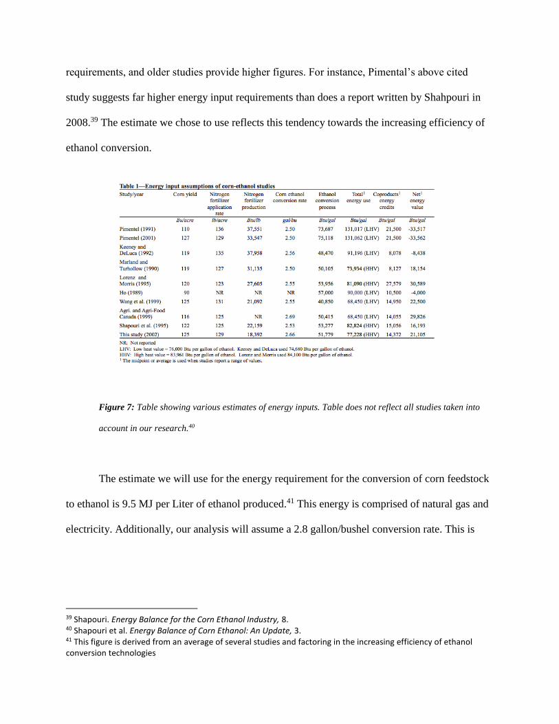
requirements, and older studies provide higher figures. For instance, Pimental’s above cited

study suggests far higher energy input requirements than does a report written by Shahpouri in

2008.39 The estimate we chose to use reflects this tendency towards the increasing efficiency of

ethanol conversion.

Figure 7: Table showing various estimates of energy inputs. Table does not reflect all studies taken into

account in our research.40

The estimate we will use for the energy requirement for the conversion of corn feedstock

to ethanol is 9.5 MJ per Liter of ethanol produced.41 This energy is comprised of natural gas and

electricity. Additionally, our analysis will assume a 2.8 gallon/bushel conversion rate. This is

39 Shapouri. Energy Balance for the Corn Ethanol Industry, 8. 40 Shapouri et al. Energy Balance of Corn Ethanol: An Update, 3. 41 This figure is derived from an average of several studies and factoring in the increasing efficiency of ethanol conversion technologies

based also on improving technologies, and that the average conversion rate stood at 2.76 gal/bu

in 2006, and has been growing steadily over the past decade and a half.42

Taking all this together, we have a total energy input:

1.55GJ/ton + 2.18 GJ/ton + 3.47 GJ/ton43 = 7.2 GJ/ton

This gives us an estimate of the energy needed to grow, harvest, transport, and convert

into ethanol, one ton of corn. An analysis of the energy balance of corn/ethanol production will

follow, but first, we will perform the above analysis on sugarcane ethanol production.

Conversion of Sugarcane into Ethanol: Energy Inputs

In the analysis of the energy inputs required for the conversion of sugarcane into ethanol,

we were able to draw from an excellent study by Coelho et al. A table created by the research

team presents two breakdowns of the energy inputs required: one for the average Brazilian cane

mill, and the other representing the most efficient of the Brazilian cane mills.

42 Groode and Heywood. Ethanol: A Look Ahead, 13. 43 2.76 gal/bu = 2.76gal/56lbs = 10.45L/56lbs = 365.63L/ton * 9.5 MJ/L = 3474.63 MJ/ton = 3.47GJ/ton

Figure 8: Energy Inputs required for ethanol conversion at average (1) and most efficient (2) sugarcane mills44

The figures listed above are extremely helpful, although need some adjusting, due to

near-decade lapse since their measurement. As with corn production and conversion, the

processes for growing and converting sugarcane into ethanol have been steadily becoming

increasingly efficient. Therefore, it stands to reason that the energy inputs in 2015 to produce a

gallon of ethanol have decreased, and our figures will reflect that. For the purposes of our

analysis, we used:

.19 GJ/ton45 + .038 GJ/ton = .228 GJ/ton

This energy requirement is remarkably lower than the requirement for corn ethanol. This

stems from the way that sugarcane ethanol is distilled. When the sugar is extracted from the

sugarcane, a byproduct called “bagasse” is created. The bagasse can itself be used as a biofuel,

and is used to fuel the distillation process. Coelho et al. included the 0 KJ/ton input from

electricity in ethanol production in their table to illustrate this effect. Once the sugarcane arrives

44 Coelho et al. Brazilian Sugarcane Ethanol, 28. 45 190,000 KJ/ton = .19 GJ/ton; this figure includes transportation as well as cultivation and harvest

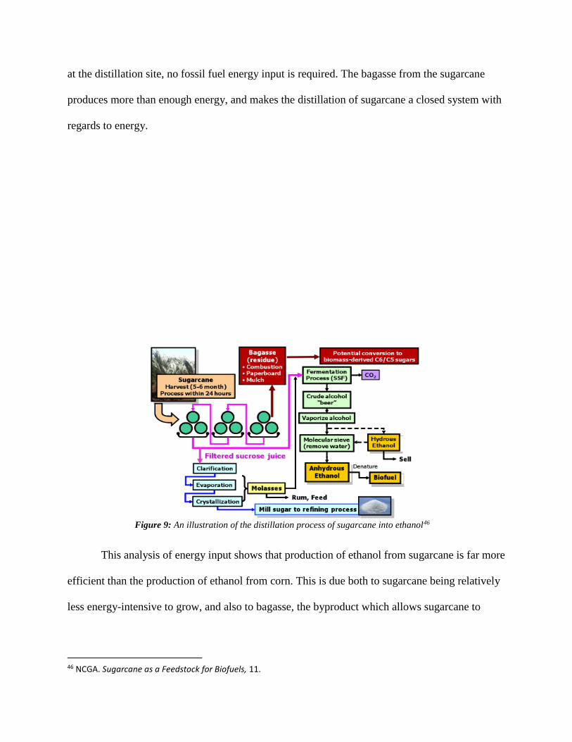
at the distillation site, no fossil fuel energy input is required. The bagasse from the sugarcane

produces more than enough energy, and makes the distillation of sugarcane a closed system with

regards to energy.

Figure 9: An illustration of the distillation process of sugarcane into ethanol46

This analysis of energy input shows that production of ethanol from sugarcane is far more

efficient than the production of ethanol from corn. This is due both to sugarcane being relatively

less energy-intensive to grow, and also to bagasse, the byproduct which allows sugarcane to

46 NCGA. Sugarcane as a Feedstock for Biofuels, 11.

power its own conversion to ethanol. While corn-ethanol has been much maligned for it

inefficiency, it appears that sugarcane – at least from an energy standpoint – provides a superior

alternative source for ethanol.

Energy Inputs Required to Produce Crude Oil

As this paper aims to provide a cost-benefit analysis of the production and consumption

of ethanol-based biofuel against the production and consumption of traditional unleaded

gasoline, a brief study of the latter is required.

There has, unsurprisingly, been much research conducted on the topic of energy input

required to extract crude oil. There are many different kinds of crude oil sources, as well as many

different kinds of extraction methods. Convening a consensus of several studies, we will use

1,280 MJ/barrel as the total energy required to extract (331 MJ), transport (880 MJ), and refine

(70 MJ), one barrel of crude oil into unleaded gasoline.4748 This translates to .0081 GJ/L of oil.

This compares to .0095 GJ/L for corn-ethanol, and .0031 GJ/L for sugarcane-ethanol. The

energy efficiency of the production of gasoline is slightly better than corn, but worse than

sugarcane by a factor of more than 2.

Energy Density of Ethanol vs. Gasoline

The paper thus far has focused on the energy inputs necessary to produce each fuel. In

this section, we will turn to the energy outputs produced by each fuel. Namely, we will compare

47 Glanfield Jr. Energy Required to Extract Petroleum Products, 33 48 In this paper, we will deal only with estimates for U.S. oil.

the energy density of each fuel, and note the corresponding change in fuel consumption that

different levels of energy density necessitate.

It is broadly known that ethanol contains roughly 67% of the energy density that gasoline

does. This means that 1 gallon of ethanol will produce 67% less energy than 1 gallon of gasoline.

As seen in the figure below, this translates fairly simply to an increase in fuel consumption rate

as the proportion of ethanol blended into the gasoline increases.

Figure 10: Charts fuel consumption rate against percentage of ethanol content in fuel. Shown at different rpm49

49 Al-Hasan. Effect of Ethanol-unleaded Gasoline Blends on Performance, 1551

Comparing this with our findings from previous sections where we determined the energy

input for a given liter of corn-ethanol, sugarcane-ethanol, and gasoline; and taking into account

that 67% more ethanol must be consumed to generate the same amount of energy; we can derive

relative energy input figures that reflect ethanol’s deficiency in energy density. The new figures

for ethanol are .0143 GJ/adjusted-L for corn-ethanol, and .0047 GJ/adjusted-L for sugarcane-

ethanol. Gasoline remains unchanged, at .0081 GJ/L. Corn-ethanol, which was already less

energy efficient to produce than gasoline, falls even further behind gasoline; yet, sugarcane-

ethanol remains more energy efficient to produce even under our new constraints.

Comparison of Emissions from Ethanol vs. Gasoline

Ethanol’s selling point is obviously not energy density – though sugarcane-ethanol did

prove more energy efficient under our analysis than traditional unleaded gaslone. Instead, a

primary virtue of ethanol is that it alleges to burn cleaner than petroleum-based fuels, thereby

providing a similar level of energy output with reduced negative externalities. This, for the most

part, is borne out in the data. Research shows GHG emissions fall as the ethanol content in fuel

increases.

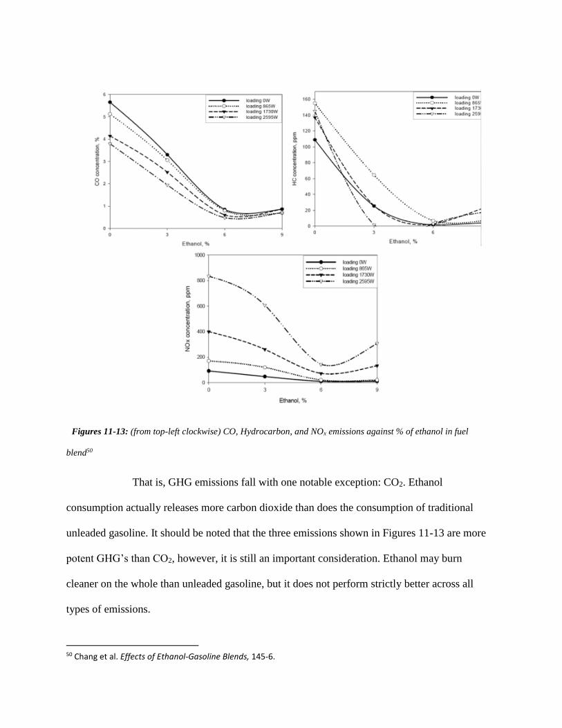
Figures 11-13: (from top-left clockwise) CO, Hydrocarbon, and NOx emissions against % of ethanol in fuel

blend50

That is, GHG emissions fall with one notable exception: CO2. Ethanol

consumption actually releases more carbon dioxide than does the consumption of traditional

unleaded gasoline. It should be noted that the three emissions shown in Figures 11-13 are more

potent GHG’s than CO2, however, it is still an important consideration. Ethanol may burn

cleaner on the whole than unleaded gasoline, but it does not perform strictly better across all

types of emissions.

50 Chang et al. Effects of Ethanol-Gasoline Blends, 145-6.

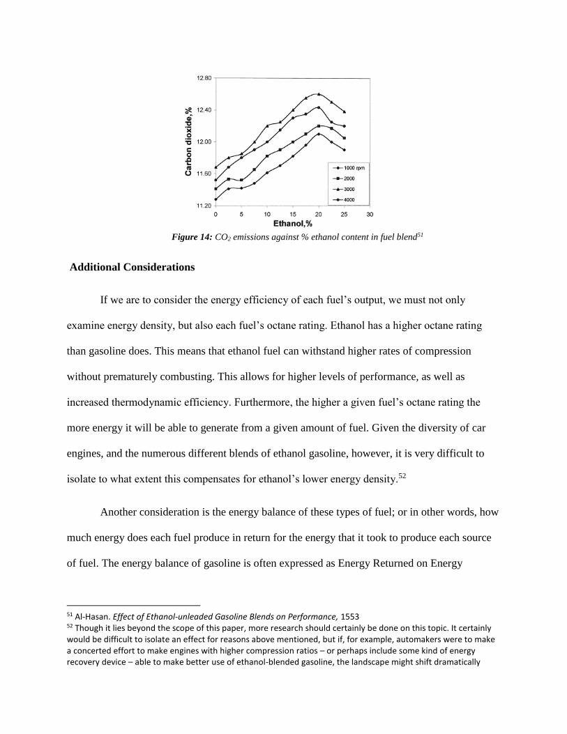
Figure 14: CO2 emissions against % ethanol content in fuel blend51

Additional Considerations

If we are to consider the energy efficiency of each fuel’s output, we must not only

examine energy density, but also each fuel’s octane rating. Ethanol has a higher octane rating

than gasoline does. This means that ethanol fuel can withstand higher rates of compression

without prematurely combusting. This allows for higher levels of performance, as well as

increased thermodynamic efficiency. Furthermore, the higher a given fuel’s octane rating the

more energy it will be able to generate from a given amount of fuel. Given the diversity of car

engines, and the numerous different blends of ethanol gasoline, however, it is very difficult to

isolate to what extent this compensates for ethanol’s lower energy density.52

Another consideration is the energy balance of these types of fuel; or in other words, how

much energy does each fuel produce in return for the energy that it took to produce each source

of fuel. The energy balance of gasoline is often expressed as Energy Returned on Energy

51 Al-Hasan. Effect of Ethanol-unleaded Gasoline Blends on Performance, 1553 52 Though it lies beyond the scope of this paper, more research should certainly be done on this topic. It certainly would be difficult to isolate an effect for reasons above mentioned, but if, for example, automakers were to make a concerted effort to make engines with higher compression ratios – or perhaps include some kind of energy recovery device – able to make better use of ethanol-blended gasoline, the landscape might shift dramatically

Invested (EROI).53 EROI ratios can vary extremely: some oil wells out of the ground by itself,

whereas some oil takes the form of tar sands. In the former case, it would not be unreasonable to

see an EROI of 100:1; in the latter, it would not be unreasonable to see an EROI in the single

digits. As oil consumption continues at a precipitous rate, EROI continues to drop, as

conventional sources of crude oil become fewer in number and more difficult to find.54

On the other hand, ethanol (both corn- and sugarcane-) has been experiencing increasing

net energy balance over the past decade. Based on our research, corn-ethanol generally returns

around a 2.5-fold increase in energy, and sugarcane-ethanol returns between an 8 and a 10-fold

increase in energy.55 Both figures should continue to rise as technology continues to improve the

distillation process.

Ethanol vs. Gasoline

Based on a relatively cursory body of research, this paper will stop short of making

normative prescriptions. However, we will conclude this section of the paper with a ranking of

the examined fuel sources, based on their energy efficiency and energy balance. Corn-ethanol

clearly lagged behind unleaded gasoline and sugarcane-ethanol. It is far more energy-intensive to

produce than both gasoline and especially sugarcane-ethanol. Moreover, the bagasse that is a

byproduct of the sugarcane distillation process now provides more energy than is needed to

power sugarcane conversion to ethanol, and so is being sold off, further offsetting production

costs. In light of this, sugarcane-ethanol is the most efficient fuel of the three.

53 Transportation Fuels and Policy, Energy of Extraction. 54 Ibid. 55 Coelho et al. Brazilian Sugarcane Ethanol, 28.

Renewable Identification Numbers and Their Effect on the Biofuel Industry

The Renewable Identification Number (RIN) system was created as a result of the United

States Environmental Protection Agency’s Renewable Fuel Standard (RFS), implemented

according to the Energy Policy Act of 2005. Each year, the United States Congress decides on a

quota of biofuel that must be produced and blended into gasoline and diesel. The RIN itself is a

serial number assigned to a batch of biofuel for the purpose of tracking its production, use, and

trading as required by the RFS. At its inception, the RIN program was initially meant to benefit

the refining industry by providing fuel producers an alternative to biofuel production. For

example, a refiner without the infrastructural capacity to produce biofuel has the option to

replace its mandate with a series of RINs. RINs may be obtained by two methods: a batch may

be separated from its original biofuel and retired as part of an obligated party’s56 quota, or a

batch may be traded openly on the market. RINs are a cleared product, mostly traded over-the-

counter, and are thus traded at a premium to factor in the cost of production of biofuel. However,

the program incurs several flaws; a qualitative analysis reveals that RIN prices are greatly

affected by biofuel mandate announcements and may incur an adversarial cost to the obligated

party. Furthermore, fraudulent RINs prove easy to produce, adding further costs to the obligated

party and inadvertently creating a buyer-beware market57.

There are five types of RINs: D3 (cellulosic biofuel), D4 (biomass-based diesel), D5

(advanced biofuel), D6 (ethanol), and D7 (cellulosic diesel). D4 and D6 RINs are the most

56 Here, the term obligated party is used to refer to the party collecting RINs for retirement to the EPA 57 A buyer-beware market requires the buyer to perform due-diligence checks before trades can be cleared

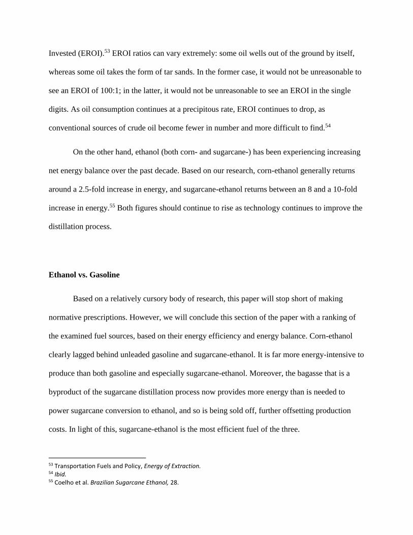
common, by virtue of their obligations as set by the EPA. A graph of the prices of D4, D5, and

D6 RINs is shown below:

Figure 1: The prices of D4, D5, and D6 RINs during the RINs price crisis of 2013

As we can see above, the price of D4 RINs is generally higher than those of the other available

RINs. In times of price shocks, we see the prices of all RINs converge, as obligated parties

become less picky about which types of RINs they would like to retire. In order to understand

this dynamic, we must first understand some of the rules of the regulation for RINs retirement.

Each obligated party is required to retire a quota of RINs at the start of the calendar

year—RINs quotas are finalized in May. The system incurs a two-year delay. For example, the

quota for 2014 RINs may be finalized in May of 2015, and an obligated party will retire RINs to

meet its quota in January of 2016. For this reason, the EPA offers several retirement

allowances58:

1. Obligated parties may retire a limited amount of RINs created two years prior to the

current year quota, and a limited amount created one year prior to the current year quota.

2. Obligated parties are required to commit a specified quota of each type of RIN, and may

satisfy the rest of its quota by any other RIN.

58 ICCT Policy Update Number 6, U.S. EPA Renewable Fuel Standard 2.

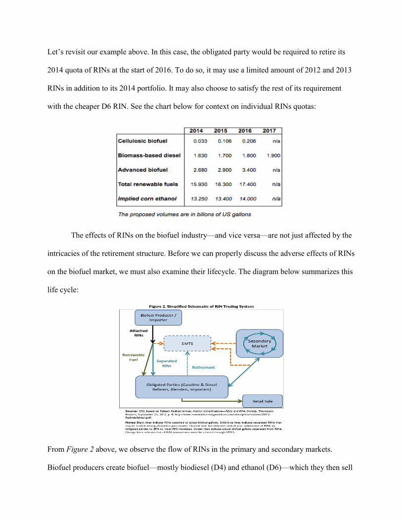
Let’s revisit our example above. In this case, the obligated party would be required to retire its

2014 quota of RINs at the start of 2016. To do so, it may use a limited amount of 2012 and 2013

RINs in addition to its 2014 portfolio. It may also choose to satisfy the rest of its requirement

with the cheaper D6 RIN. See the chart below for context on individual RINs quotas:

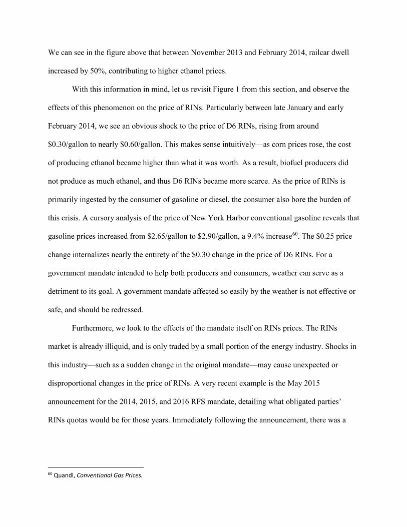
The effects of RINs on the biofuel industry—and vice versa—are not just affected by the

intricacies of the retirement structure. Before we can properly discuss the adverse effects of RINs

on the biofuel market, we must also examine their lifecycle. The diagram below summarizes this

life cycle:

From Figure 2 above, we observe the flow of RINs in the primary and secondary markets.

Biofuel producers create biofuel—mostly biodiesel (D4) and ethanol (D6)—which they then sell

to obligated parties, consisting of renders and blenders. The obligated parties then blend this

biofuel into their product, and sell the finished gasoline and/or diesel to the retail market. During

this process, the attached RINs are separated, and may be retired to the EPA. They also may be

sold into the secondary market, from which the obligated party may buy detached RINs to retire.

There is one key step missing in this diagram—the production of the corn, soybean, or

sugar used to create the biofuel. Producers are unable to create biofuel without the necessary

agricultural inputs. Thus, it is possible that a shortage of these inputs—such as corn—may

increase the cost of biofuel production, and inadvertently increase the price of RINs.

Additionally, corn ethanol is transported by railcar. The combination of these two factors make

the RINs market susceptible to bad weather, primarily in the winter when cold temperatures can

reduce crop yield and heavy snows and congest rail traffic. This is precisely what happened in

early 2014. Between the months of January and March 2014, Chicago spot ethanol prices

increased over 74% due to brutally cold weather delaying train traffic. See Figure 3 below59:

Figure 3: This figure depicts train speed and dwell time, causing the spike in ethanol prices in early 2014.

59 EIA, Rail Congestion, Cold Weather Affect Ethanol Spot Prices.

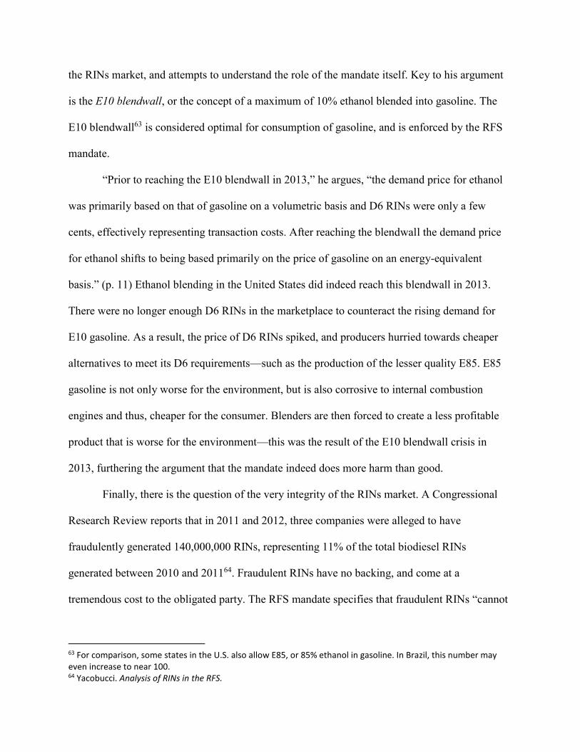
We can see in the figure above that between November 2013 and February 2014, railcar dwell

increased by 50%, contributing to higher ethanol prices.

With this information in mind, let us revisit Figure 1 from this section, and observe the

effects of this phenomenon on the price of RINs. Particularly between late January and early

February 2014, we see an obvious shock to the price of D6 RINs, rising from around

$0.30/gallon to nearly $0.60/gallon. This makes sense intuitively—as corn prices rose, the cost

of producing ethanol became higher than what it was worth. As a result, biofuel producers did

not produce as much ethanol, and thus D6 RINs became more scarce. As the price of RINs is

primarily ingested by the consumer of gasoline or diesel, the consumer also bore the burden of

this crisis. A cursory analysis of the price of New York Harbor conventional gasoline reveals that

gasoline prices increased from $2.65/gallon to $2.90/gallon, a 9.4% increase60. The $0.25 price

change internalizes nearly the entirety of the $0.30 change in the price of D6 RINs. For a

government mandate intended to help both producers and consumers, weather can serve as a

detriment to its goal. A government mandate affected so easily by the weather is not effective or

safe, and should be redressed.

Furthermore, we look to the effects of the mandate itself on RINs prices. The RINs

market is already illiquid, and is only traded by a small portion of the energy industry. Shocks in

this industry—such as a sudden change in the original mandate—may cause unexpected or

disproportional changes in the price of RINs. A very recent example is the May 2015

announcement for the 2014, 2015, and 2016 RFS mandate, detailing what obligated parties’

RINs quotas would be for those years. Immediately following the announcement, there was a

60 Quandl, Conventional Gas Prices.

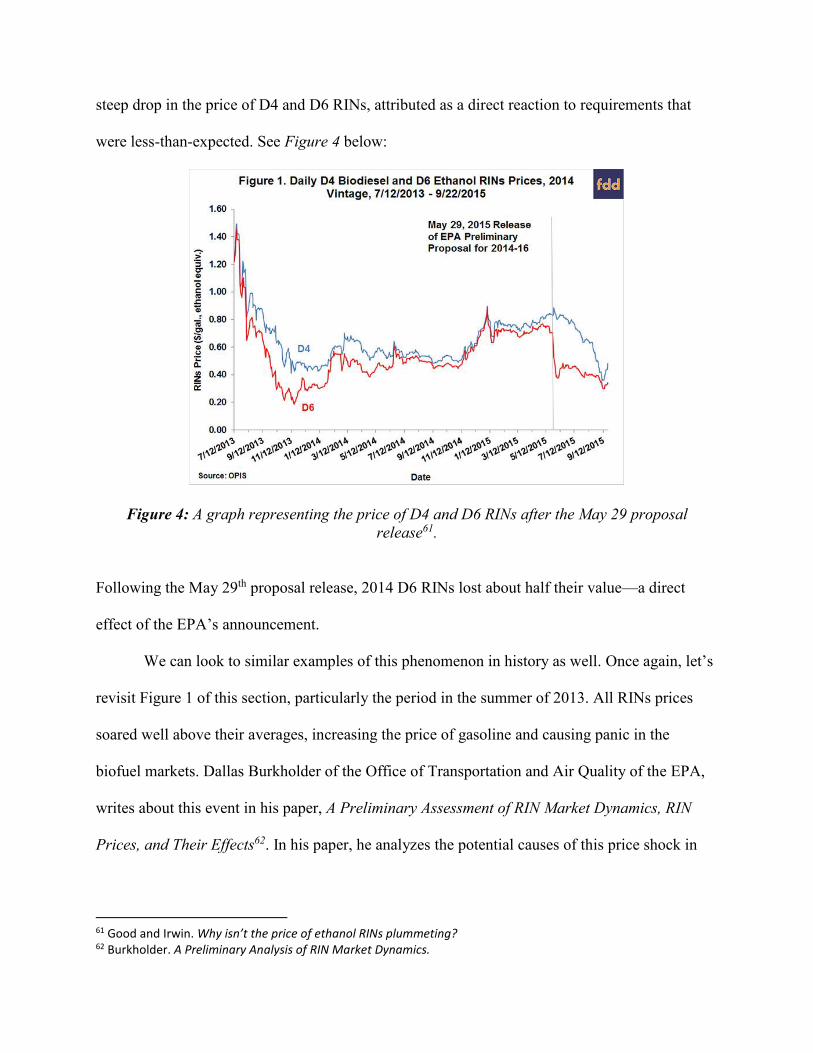
steep drop in the price of D4 and D6 RINs, attributed as a direct reaction to requirements that

were less-than-expected. See Figure 4 below:

Figure 4: A graph representing the price of D4 and D6 RINs after the May 29 proposal

release61.

Following the May 29th proposal release, 2014 D6 RINs lost about half their value—a direct

effect of the EPA’s announcement.

We can look to similar examples of this phenomenon in history as well. Once again, let’s

revisit Figure 1 of this section, particularly the period in the summer of 2013. All RINs prices

soared well above their averages, increasing the price of gasoline and causing panic in the

biofuel markets. Dallas Burkholder of the Office of Transportation and Air Quality of the EPA,

writes about this event in his paper, A Preliminary Assessment of RIN Market Dynamics, RIN

Prices, and Their Effects62. In his paper, he analyzes the potential causes of this price shock in

61 Good and Irwin. Why isn’t the price of ethanol RINs plummeting? 62 Burkholder. A Preliminary Analysis of RIN Market Dynamics.

the RINs market, and attempts to understand the role of the mandate itself. Key to his argument

is the E10 blendwall, or the concept of a maximum of 10% ethanol blended into gasoline. The

E10 blendwall63 is considered optimal for consumption of gasoline, and is enforced by the RFS

mandate.

“Prior to reaching the E10 blendwall in 2013,” he argues, “the demand price for ethanol

was primarily based on that of gasoline on a volumetric basis and D6 RINs were only a few

cents, effectively representing transaction costs. After reaching the blendwall the demand price

for ethanol shifts to being based primarily on the price of gasoline on an energy-equivalent

basis.” (p. 11) Ethanol blending in the United States did indeed reach this blendwall in 2013.

There were no longer enough D6 RINs in the marketplace to counteract the rising demand for

E10 gasoline. As a result, the price of D6 RINs spiked, and producers hurried towards cheaper

alternatives to meet its D6 requirements—such as the production of the lesser quality E85. E85

gasoline is not only worse for the environment, but is also corrosive to internal combustion

engines and thus, cheaper for the consumer. Blenders are then forced to create a less profitable

product that is worse for the environment—this was the result of the E10 blendwall crisis in

2013, furthering the argument that the mandate indeed does more harm than good.

Finally, there is the question of the very integrity of the RINs market. A Congressional

Research Review reports that in 2011 and 2012, three companies were alleged to have

fraudulently generated 140,000,000 RINs, representing 11% of the total biodiesel RINs

generated between 2010 and 201164. Fraudulent RINs have no backing, and come at a

tremendous cost to the obligated party. The RFS mandate specifies that fraudulent RINs “cannot

63 For comparison, some states in the U.S. also allow E85, or 85% ethanol in gasoline. In Brazil, this number may even increase to near 100. 64 Yacobucci. Analysis of RINs in the RFS.

be used to achieve compliance with the Renewable Volume Obligation (RVO) of an obligated

party or exporter, regardless of the party’s good faith belief that the RINs were valid at the time

they were acquired.” This language reinforces this “buyer-beware” system, in which the buyer of

the RINs is forced to perform due diligence checks on the seller before any transaction. On top of

the additional legal costs of due diligence, obligated parties bear an expensive burden in case

they unknowingly retire fraudulent RINs:

“1. the original cost of the fraudulent RINs (spot prices ranged between $0.70 and $2.00 per RIN

over that time);

2. penalties to EPA for Clean Air Act violations ($0.10 per RIN, capped at $350,000 per party);

3. the cost of all make-up RINs (trading at the time of settlement at roughly $0.50 per gallon);

and

4. any legal costs in pursuing restitution from fraudulent actors.” (p. 11)

The market for Renewable Identification Numbers was originally created to provide

obligated parties with the flexibility of blending biofuel into gasoline, or going out onto the

market to purchase the RINs necessary for its requirement. However, as this paper demonstrates,

there are many holes in this system that are an active detriment to the obligated parties. Sudden

changes in requirements, factors beyond government control such as the weather, and the very

integrity of RINs themselves all provide reason as to why this system is flawed and should be

redressed. Of course, as this paper argues, RINs are a small piece of a larger problem that is

biofuel mandates in general, which cause more harm than good to the producer, the consumer,

and the planet.

Conclusion and Further Questions

We sought out to reexamine biofuel mandates in the United States and Brazil, in order to

determine their efficacy and understand the possible negative externalities. In order to do so, we

looked at several key indicators of performance of biofuel mandates in these two countries, as

well as industries that could potentially be harmed by their unintended consequences. Previous

literature suggests that ethanol prices greatly impact the price of its agricultural inputs—such as

corn—with statistical significance. Therefore, we started by testing this claim with OLS

regression.

Several challenges arose with the data, regarding its granularity and non-stationary

properties. In order to conform the data to meet the requirements of OLS regression, it was

necessary to treat it appropriately. Following treatment and testing of the data, we determined

that there was no statistically significant evidence to prove the claim that corn prices are affected

by ethanol production, as a result of biofuel mandates. However, we did find qualitative evidence

to support the claim that biofuel production could have a negative impact on corn prices given

certain conditions, such as the weather. We consider this a weakness in the Renewable Fuel

Standard, and one reason why it should be re-evaluated.

We also analyzed the redistribution of land usage before and after the biofuel mandates

were set in place. In the United States, corn’s share of land usage has increased tremendously,

coinciding with the expansion of the Renewable Fuel Standard. Additionally, the amount of corn

used in the production of ethanol has grown exponentially. However, there is a common

misconception that corn production for ethanol directly takes away from corn used for feedstock.

In our analysis, we concluded that corn used in the production of biofuels is an entirely separate

type of corn, and cannot be consumed. Therefore, while land usage changes are an indirect

consequence of biofuel mandates, this proven misconception sheds important light on their

effects on agricultural prices.

Relative energy efficiency was an important consideration in our analysis of the costs of

biofuel mandates. We compared the energy inputs for conversion of corn and sugarcane into

ethanol, crude into gasoline, and the energy densities of ethanol compared to gasoline. Through

our analysis, we determined that the production of corn ethanol net consumes energy, and that

gasoline is strongly preferred. However, we also determined that the production of sugarcane

ethanol has a higher yield potential than that of gasoline. In fact, in an analysis of the three fuels,

sugarcane ethanol provides the greatest energy output for its inputs. Given that the comparison of

ethanol emissions and gasoline emissions yielded a relatively zero-sum game, we can conclude

that sugarcane ethanol is indeed the better choice. However, the share of ethanol production in

the United States is dominated by corn ethanol, which lags behind gasoline. In essence, this

result is good for the Brazilian ethanol industry, and is more of a negative externality than its

worth for the American ethanol industry.

In order to reaffirm this conclusion, we more deeply analyzed Brazil, and the effects of

biofuel mandates on its country. We determined that sugarcane ethanol is the ideal choice over

corn ethanol and gasoline, but we wanted to ensure that Brazil was not harmed by its own biofuel

mandates. Through our analysis, we discovered that the Brazilian economy has benefited

tremendously from the production of sugarcane ethanol, and the introduction of flex-fuel

vehicles. The country managed to provide energy self-sustainability to its people, and also rise as

the world’s second largest exporter of ethanol. However, one further question to examine is how

Brazil’s economy may rely on its ethanol industry—that is, if the industry did not do well, would

the economy suffer with it. Exogenous factors such as weather also come into play. This is not

the scope of this paper, but we can claim from our analysis that biofuel mandates in Brazil have

been more beneficial than harmful.

We conclude by reaffirming our claim—the costs of biofuel mandates in the United

States largely outweigh the benefits. This claim does not hold in Brazil, however. The economic,

legislative, and ethical effects of the Renewable Fuel Standard simply do not provide enough

backing to the consumer or the producer, as exemplified by our analysis. In particular, the

Renewable Identification Numbers trading system comes at a huge burden to the obligated

parties—the target the program was supposed to have helped. As a result of our analysis, the

Renewable Fuel Standard in particular, should be reevaluated.

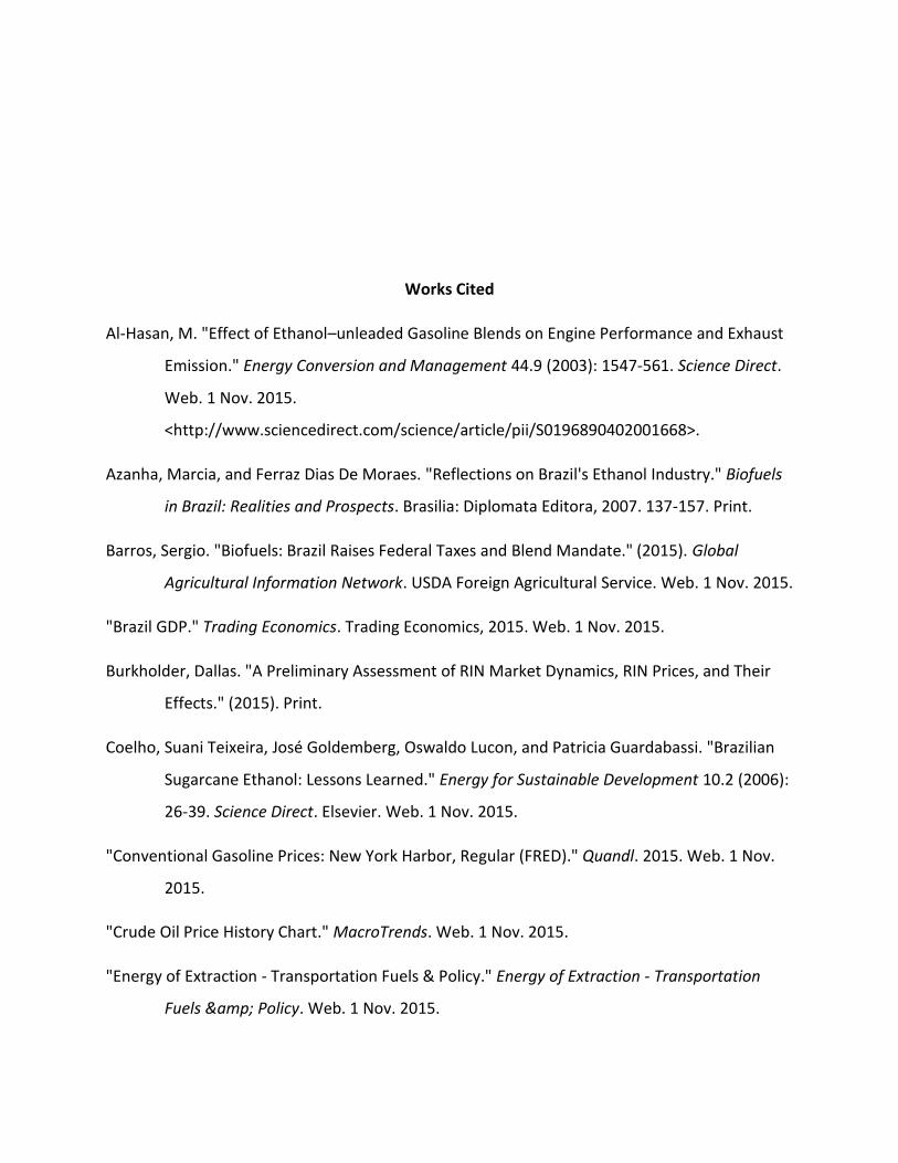
Works Cited

Al-Hasan, M. "Effect of Ethanol–unleaded Gasoline Blends on Engine Performance and Exhaust

Emission." Energy Conversion and Management 44.9 (2003): 1547-561. Science Direct.

Web. 1 Nov. 2015.

<http://www.sciencedirect.com/science/article/pii/S0196890402001668>.

Azanha, Marcia, and Ferraz Dias De Moraes. "Reflections on Brazil's Ethanol Industry." Biofuels

in Brazil: Realities and Prospects. Brasilia: Diplomata Editora, 2007. 137-157. Print.

Barros, Sergio. "Biofuels: Brazil Raises Federal Taxes and Blend Mandate." (2015). Global

Agricultural Information Network. USDA Foreign Agricultural Service. Web. 1 Nov. 2015.

"Brazil GDP." Trading Economics. Trading Economics, 2015. Web. 1 Nov. 2015.

Burkholder, Dallas. "A Preliminary Assessment of RIN Market Dynamics, RIN Prices, and Their

Effects." (2015). Print.

Coelho, Suani Teixeira, José Goldemberg, Oswaldo Lucon, and Patricia Guardabassi. "Brazilian

Sugarcane Ethanol: Lessons Learned." Energy for Sustainable Development 10.2 (2006):

26-39. Science Direct. Elsevier. Web. 1 Nov. 2015.

"Conventional Gasoline Prices: New York Harbor, Regular (FRED)." Quandl. 2015. Web. 1 Nov.

2015.

"Crude Oil Price History Chart." MacroTrends. Web. 1 Nov. 2015.

"Energy of Extraction - Transportation Fuels & Policy." Energy of Extraction - Transportation

Fuels &amp; Policy. Web. 1 Nov. 2015.

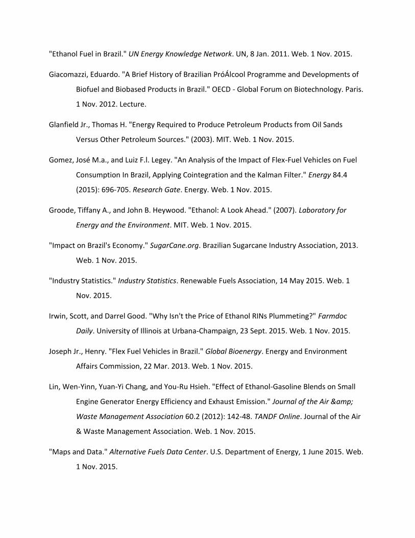
"Ethanol Fuel in Brazil." UN Energy Knowledge Network. UN, 8 Jan. 2011. Web. 1 Nov. 2015.

Giacomazzi, Eduardo. "A Brief History of Brazilian PróÁlcool Programme and Developments of

Biofuel and Biobased Products in Brazil." OECD - Global Forum on Biotechnology. Paris.

1 Nov. 2012. Lecture.

Glanfield Jr., Thomas H. "Energy Required to Produce Petroleum Products from Oil Sands

Versus Other Petroleum Sources." (2003). MIT. Web. 1 Nov. 2015.

Gomez, José M.a., and Luiz F.l. Legey. "An Analysis of the Impact of Flex-Fuel Vehicles on Fuel

Consumption In Brazil, Applying Cointegration and the Kalman Filter." Energy 84.4

(2015): 696-705. Research Gate. Energy. Web. 1 Nov. 2015.

Groode, Tiffany A., and John B. Heywood. "Ethanol: A Look Ahead." (2007). Laboratory for

Energy and the Environment. MIT. Web. 1 Nov. 2015.

"Impact on Brazil's Economy." SugarCane.org. Brazilian Sugarcane Industry Association, 2013.

Web. 1 Nov. 2015.

"Industry Statistics." Industry Statistics. Renewable Fuels Association, 14 May 2015. Web. 1

Nov. 2015.

Irwin, Scott, and Darrel Good. "Why Isn't the Price of Ethanol RINs Plummeting?" Farmdoc

Daily. University of Illinois at Urbana-Champaign, 23 Sept. 2015. Web. 1 Nov. 2015.

Joseph Jr., Henry. "Flex Fuel Vehicles in Brazil." Global Bioenergy. Energy and Environment

Affairs Commission, 22 Mar. 2013. Web. 1 Nov. 2015.

Lin, Wen-Yinn, Yuan-Yi Chang, and You-Ru Hsieh. "Effect of Ethanol-Gasoline Blends on Small

Engine Generator Energy Efficiency and Exhaust Emission." Journal of the Air &amp;

Waste Management Association 60.2 (2012): 142-48. TANDF Online. Journal of the Air

& Waste Management Association. Web. 1 Nov. 2015.

"Maps and Data." Alternative Fuels Data Center. U.S. Department of Energy, 1 June 2015. Web.

1 Nov. 2015.

"No. 11 Sugar Futures End of Day Settlement Price." Sugar Prices. Index Mundi, 2015. Web. 1

Nov. 2015.

Nøvaes, W. S., S. H. M. Caixeta, P. V. P. Selvam, H. P. A. Santos, and G. B. Costa. "Fuel Ethanol

from Brazilian Biomass: Economic Risk Analysis Based on Monte Carlo Simulation

Techniques." Sci ELO: Proceedings 4.1 (2002). Sci ELO: Proceedings. Sci ELO:

Proceedings. Web. 1 Nov. 2015.

Pimentel, David. "Ethanol Fuels: Energy Balance, Economics, and Environmental Impacts Are

Negative." Natural Resources Research 12.2 (2003): 127-34. Energy Justice. Natural

Resources Research. Web. 1 Nov. 2015.

"Preserving Biodiversity and Protecting Precious Resources." SugarCane.org. Brazilian

Sugarcane Industry Association, 2013. Web. 1 Nov. 2015.

"Producing Food and Fuel." SugarCane.org. Brazilian Sugarcane Industry Association, 2013.

Web. 1 Nov. 2015.

"Rail Congestion, Cold Weather Raise Ethanol Spot Prices." U.S. Energy Information Association.

EIA, 3 Apr. 2014. Web. 1 Nov. 2015.

Schnepf, Randy, and Brent Yacobucci. "Renewable Fuel Standards (RFS): Overview and Issues."

UNT Digital Library. Congressional Research Service, 14 Oct. 2010. Web. 1 Nov. 2015.

Shapouri, H. 2008 Energy Balance for the Corn-Ethanol Industry. Collingdale: DIANE, 2011. 8.

Print.

Shapouri, Hosein, James A. Duffield, and Michael Wang. "The Energy Balance of Corn Ethanol:

An Update." (2002). Print.

Soccol, Carlos R., Luciana P. S. Vandenberghe, Bill Costa, and Adenise L. Woiciechowski.

"Brazilian Biofuel Program: An Overview." Journal of Scientific and Industrial Research

64.1 (2005): 897-904. NICAIR Online Periodicals Repository. NOPR. Web. 1 Nov. 2015.

"Sugarcane as a Feedstock for Biofuels." NCGA. NCGA, 1 Sept. 2009. Web. 1 Nov. 2015.

"U.S. EPA Renewable Fuel Standard 2." (2010). ICCT Policy Update Number 6. International

Council on Clean Transportation. Web. 1 Nov. 2015.

"U.S. Energy Information Administration - EIA - Independent Statistics and Analysis." Today in

Energy. U.S. Energy Information Administration, 31 Aug. 2012. Web. 1 Nov. 2015.

"USDA/NASS QuickStats." National Agricultural Statistics Service. United Stated Department of

Agriculture. Web. 3 Dec. 2015.

Valdes, Constanza. "Brazil's Ethanol Industry: Looking Forward." (2011). Economic Research

Service. United Stated Department of Agriculture. Web. 1 Nov. 2015.

Yacobucci, Brent D. "Analysis of Renewable Identification Numbers (RINs) in the Renewable

Fuel Standard (RFS)." (2013). Federation of American Scientists. Congressional Research

Service. Web. 1 Nov. 2015.

Zilberman, David, Gal Hochman, Deepak Rajagopal, Steve Sexton, and Govinda Timilsina. "The

Impact of Biofuels on Commodity Food Prices: Assessment of Findings." American

Journal of Agricultural Economics 97.5 (2012): 275-81. Oxford Journals. American

Journal of Agricultural Economics. Web. 1 Nov. 2015.

De Gorter, Harry, and David R. Just. "The Social Costs and Benefits of Biofuels: The Intersection

of Environmental, Energy and Agricultural Policy." Applied Economic Perspectives and

Policy 32.1 (2010): 4-32. Applied Economic Perspectives and Policy. Oxford Journals.

Web. 1 Nov. 2015.

MLA formatting by BibMe.org.