Embed Size (px)
Citation preview
The law of Supply
When the price of a good rises, the quantity supplied will also riseWhen the price of a good rises, the quantity supplied will also rise
1. Costs rise as output increases.
2. Higher price means more profit. Firms will switch to the production of this good from other goods.
3.New producers will emerge. Total supply will increase.
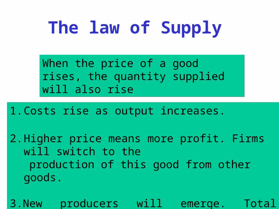
Quantity Supplied = f (Price)Quantity Supplied = f (Price)
A positive relationship exists between Qs & P
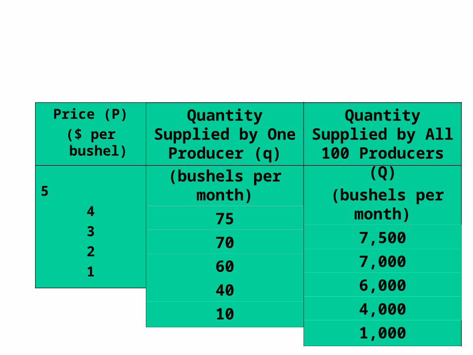
SUPPLY SCHEDULE
Supply schedule simply specifies the unit of a good that a producer is willing to supply i.e. Qs at alternative prices over a given period.

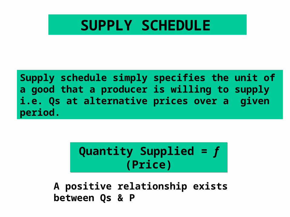
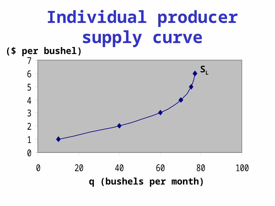
Price (P)
($ per bushel)
5
4
3
2
1
Quantity Supplied by One Producer (q)
(bushels per month)
75
70
60
40
10
Quantity Supplied by All 100 Producers (Q)
(bushels per month)
7,500
7,000
6,000
4,000
1,000
0
1
2
34
5
6
7
0 20 40 60 80 100
Individual producer supply curveP ($ per bushel)
q (bushels per month)
SL
Price (P)
($ per bushel)
5
4
3
2
1
Quantity Supplied by One Producer (q)
(bushels per month)
75
70
60
40
10
Quantity Supplied by All 100 Producers (Q)
(bushels per month)
7,500
7,000
6,000
4,000
1,000
0
1
2
34
5
6
7
0 2000 4000 6000 8000 10000
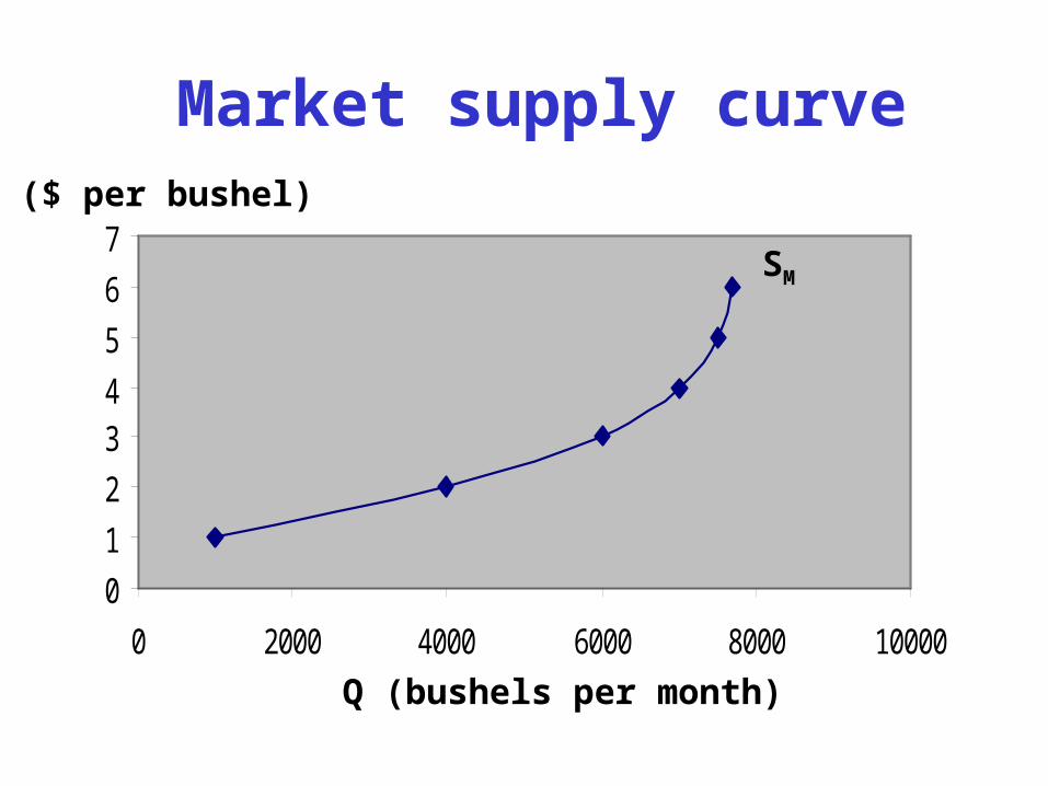
Market supply curve
SM
Q (bushels per month)
P ($ per bushel)
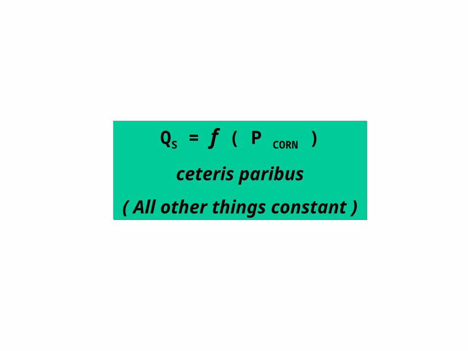
QS = f ( P CORN )
ceteris paribus
( All other things constant )
QS = f ( P CORN )
ceteris paribus
( All other things constant )
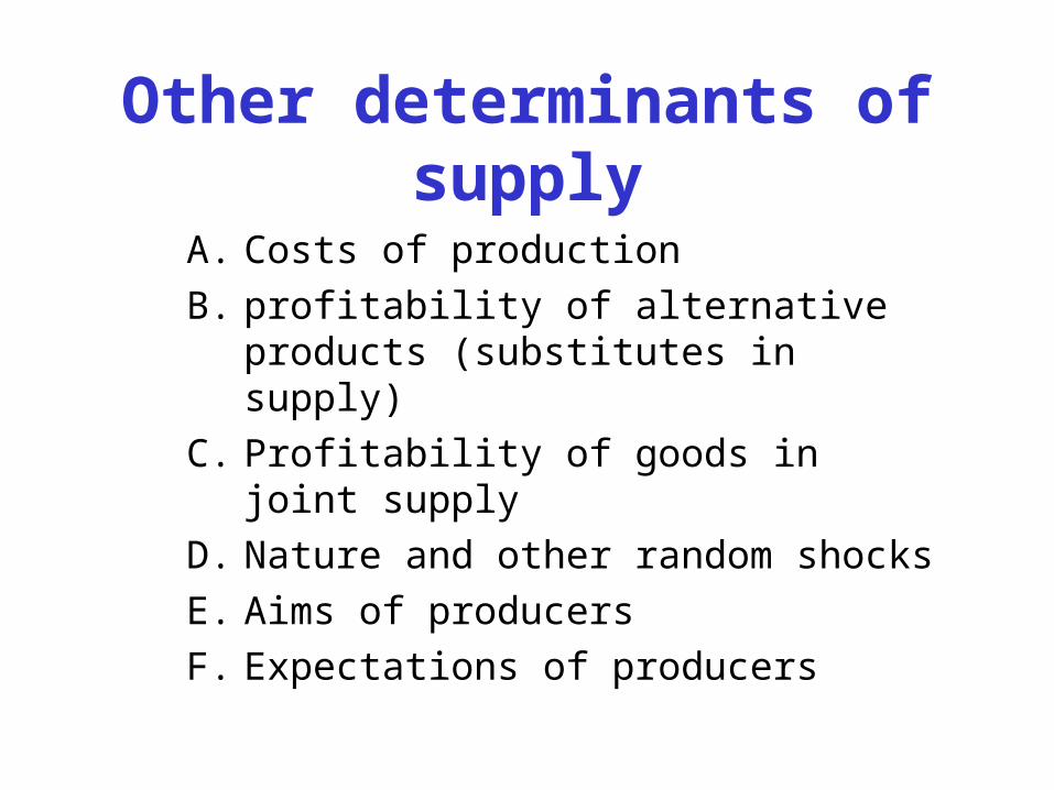
Other determinants of supply
A. Costs of production
B. profitability of alternative products (substitutes in supply)
C. Profitability of goods in joint supply
D. Nature and other random shocks
E. Aims of producers
F. Expectations of producers
A : Costs of production
If production costs change then the amount supplied is likely to change. Costs change due to :
→ Changes in input prices.
→ Changes in technology.
→ Organizational changes.
→ Changes in govt policy
B: Profitability of alternative products
(substitutes in supply)
• A producer of two goods is more likely to concentrate on the production of the more profitable good
C: Profitability of goods in joint supply
Variant on the previous case.
D: Nature and other random shocks
Problems caused by weather, natural catastrophes & effects of war, also hazards like gulabi sundi and american sundi.
E: Aims of producers
A firm may wish to maximize short run profit. The quantity supplied will obviously be affected by the aims of the producer.
F: Expectations of producers.
Expectations of increase or decrease in the price in future. Expectations may prove to be wrong.
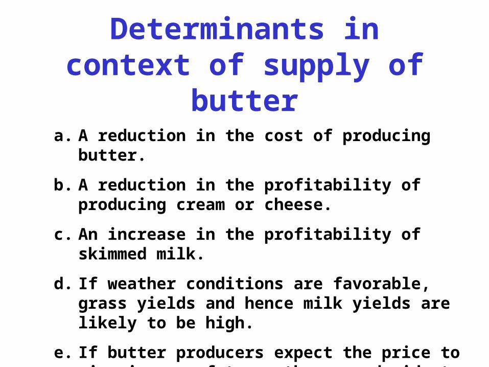
Determinants in context of supply of butter
a. A reduction in the cost of producing butter.
b. A reduction in the profitability of producing cream or cheese.
c. An increase in the profitability of skimmed milk.
d. If weather conditions are favorable, grass yields and hence milk yields are likely to be high.
e. If butter producers expect the price to rise in near future, they may decide to release less to the market now.
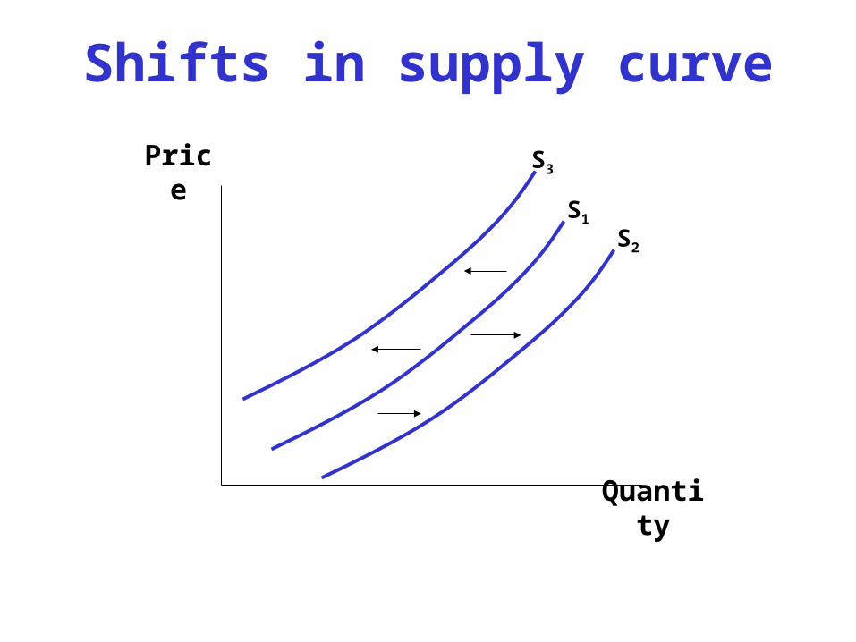
Shifts in supply curve
Quantity
S1
S2
S3Price
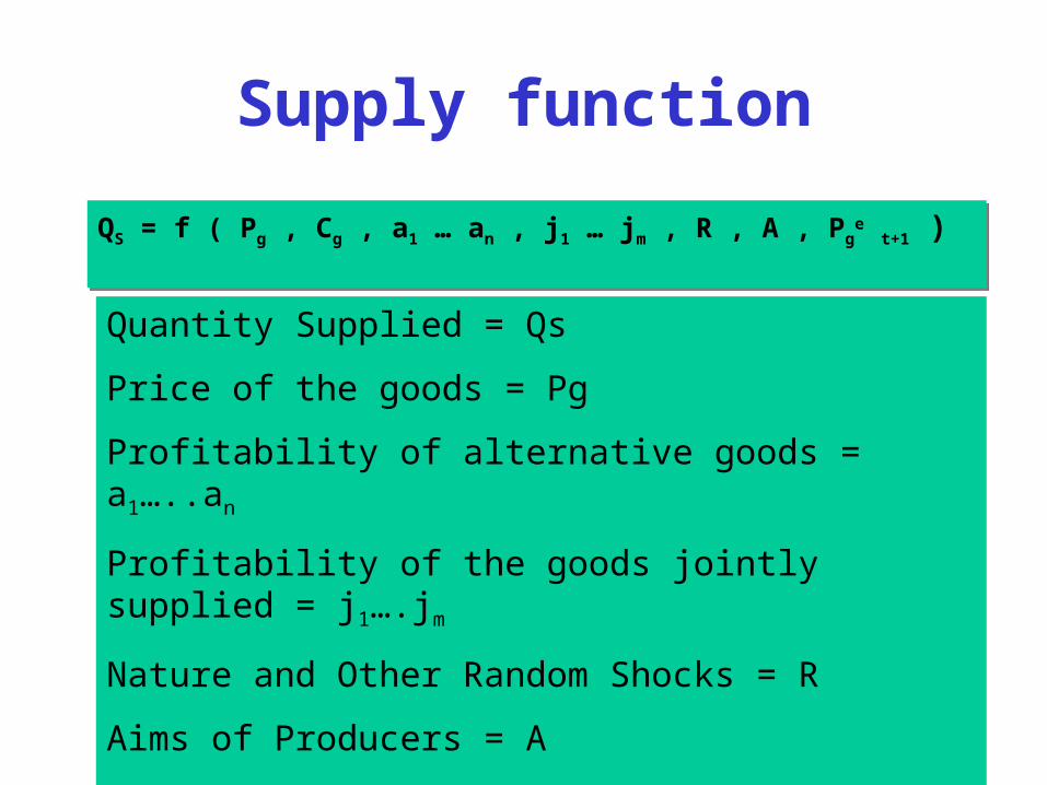
Supply function
QS = f ( Pg , Cg , a1 … an , j1 … jm , R , A , Pge t+1 )QS = f ( Pg , Cg , a1 … an , j1 … jm , R , A , Pge t+1 )
Quantity Supplied = Qs
Price of the goods = Pg
Profitability of alternative goods = a1…..an
Profitability of the goods jointly supplied = j1….jm
Nature and Other Random Shocks = R
Aims of Producers = A
Expected Price of good = Pge at some future time = t+1
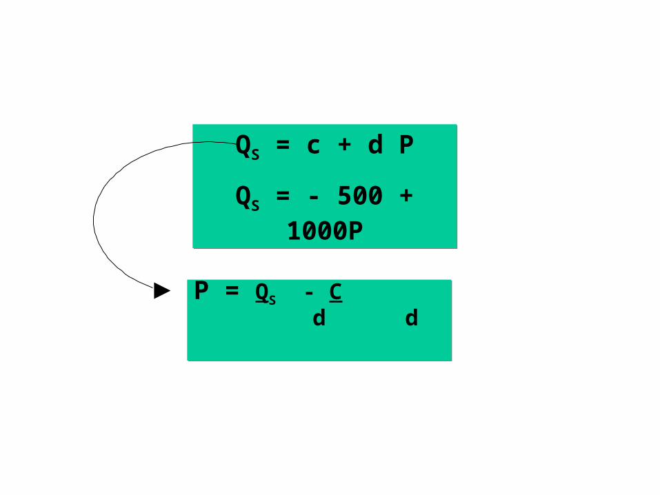
QS = c + d P
QS = - 500 + 1000P
QS = c + d P
QS = - 500 + 1000P
P = QS - C d dP = QS - C d d
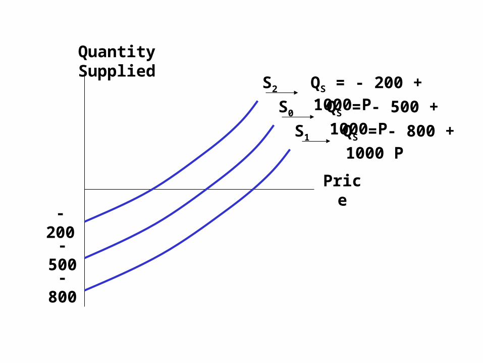
Quantity Supplied
Price
S2 QS = - 200 + 1000 P
S0 QS = - 500 + 1000 P
S1 QS = - 800 + 1000 P
-200
-500
-800
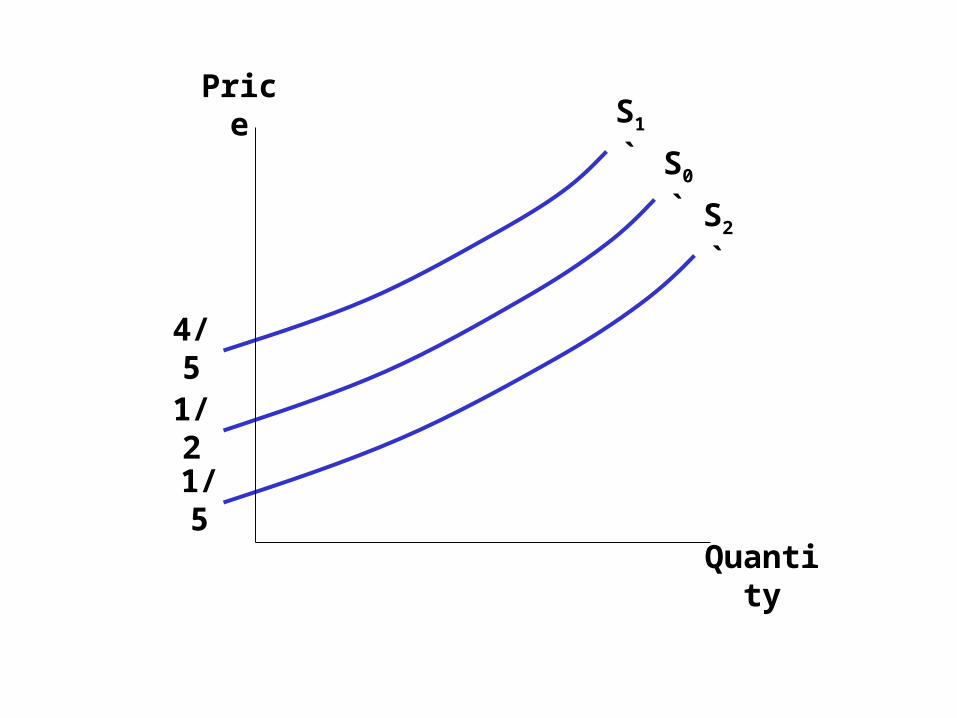
Quantity
PriceS1`
S0`
S2`
4/5
1/2
1/5
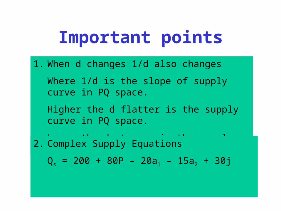
Important points
1. When d changes 1/d also changes
Where 1/d is the slope of supply curve in PQ space.
Higher the d flatter is the supply curve in PQ space.
Lower the d steeper is the supply curve in PQ space.
2. Complex Supply Equations
Qs = 200 + 80P – 20a1 – 15a2 + 30j
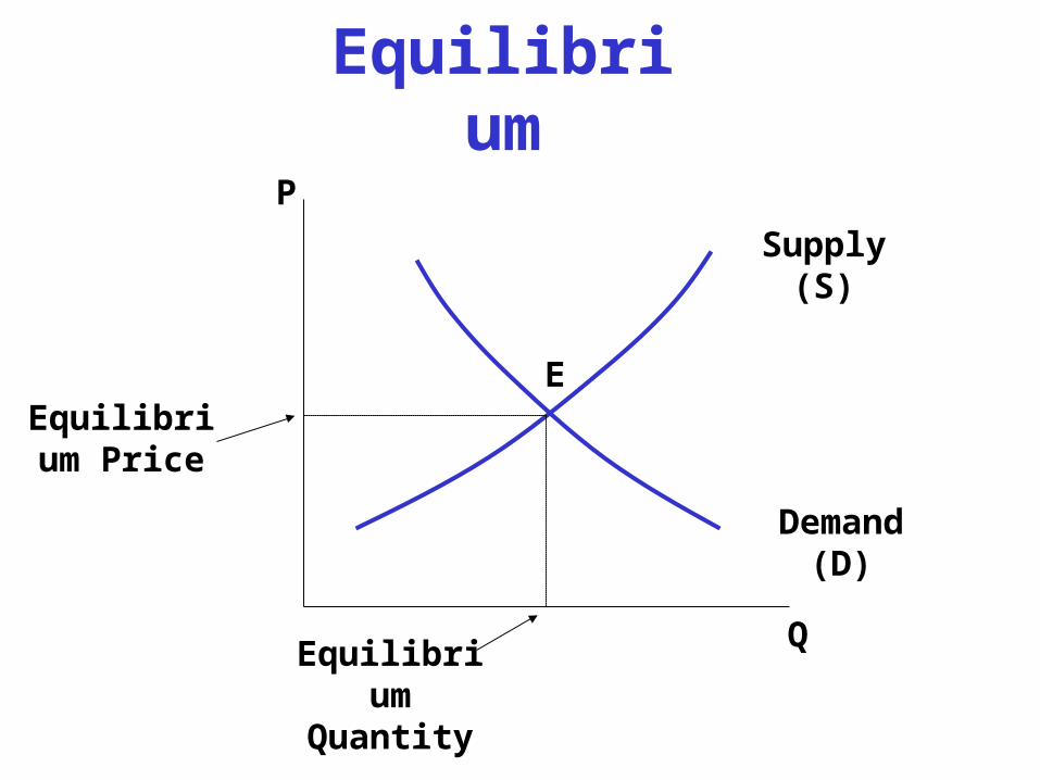
Equilibrium
EEquilibrium
Price
Equilibrium Quantity
P
Q
Supply (S)
Demand (D)
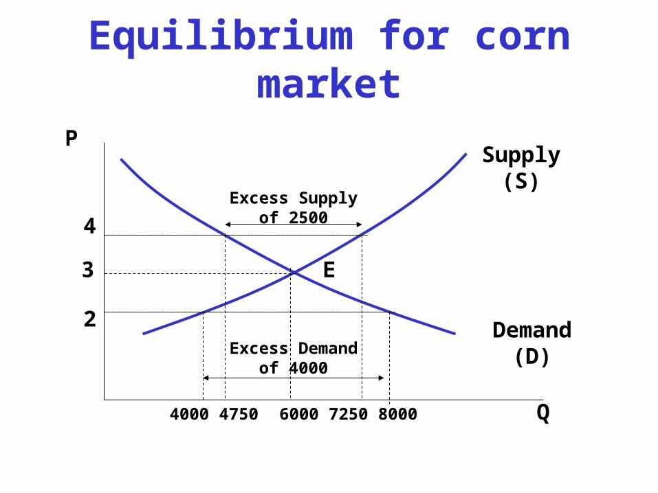
Equilibrium for corn market
Supply (S)
Demand (D)
Q
P
3
6000
E
Excess Supply of 2500
Excess Demand of 4000
4750 72504000 8000
2
4
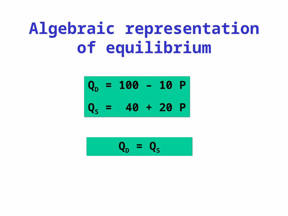
QD = 100 – 10 P
QS = 40 + 20 P
QD = 100 – 10 P
QS = 40 + 20 P
QD = QSQD = QS
Algebraic representation of equilibrium
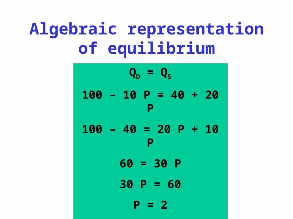
QD = QS
100 – 10 P = 40 + 20 P
100 – 40 = 20 P + 10 P
60 = 30 P
30 P = 60
P = 2
Thus equilibrium price is $2
QD = QS
100 – 10 P = 40 + 20 P
100 – 40 = 20 P + 10 P
60 = 30 P
30 P = 60
P = 2
Thus equilibrium price is $2
Algebraic representation of equilibrium
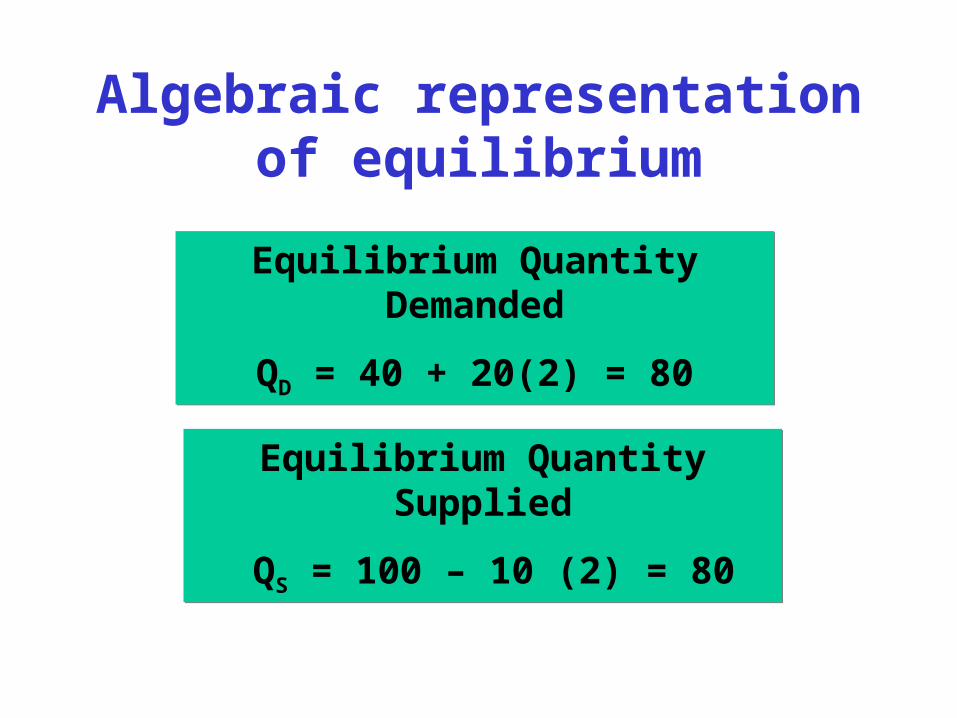
Equilibrium Quantity Demanded
QD = 40 + 20(2) = 80
Equilibrium Quantity Demanded
QD = 40 + 20(2) = 80
Equilibrium Quantity Supplied
QS = 100 – 10 (2) = 80
Equilibrium Quantity Supplied
QS = 100 – 10 (2) = 80
Algebraic representation of equilibrium