Embed Size (px)
Citation preview
The Large Time-Frequency Analysis Toolbox 2.0
Zdenek Prusa1, Peter L. Søndergaard2, Nicki Holighaus1, ChristophWiesmeyr3 and Peter Balazs1
1 Acoustics Research Institute, Austrian Academy of Sciences,Wohllebengasse 12–14, 1040 Vienna, Austria
{zdenek.prusa,nicki.holighaus,peter.balazs}@oeaw.ac.at2 Oticon A/S,
Kongebakken 9, 2765 Smørum, [email protected]
3 Numerical Harmonic Analysis Group, Faculty of Mathematics, University of ViennaOskar-Morgenstern-Platz 1, 1090 Vienna, Austria
Abstract. The Large Time Frequency Analysis Toolbox (LTFAT) isa modern Octave/Matlab toolbox for time-frequency analysis, synthe-sis, coefficient manipulation and visualization. It’s purpose is to serveas a tool for achieving new scientific developments as well as an edu-cational tool. The present paper introduces main features of the secondmajor release of the toolbox which includes: generalizations of the Gabortransform, the wavelets module, the frames framework and the real-timeblock processing framework.
Keywords: frames, Fourier transform, Gabor transform, wavelet trans-form, real-time audio processing
1 Introduction
Time-Frequency analysis is a very important tool for signal processing and itsapplications in audio, video and acoustics. It allows a representation showingsimultaneously (to some extent) the frequency and time content of a signal.Typical representations are the Gabor [16] or wavelet [17] transforms. In recentyears more flexible transforms, in the form of adapted and adaptive represen-tations were a very active topic of research, see e.g. [3]. For all those conceptsthe mathematical theory of frames has proven to be highly significant, as framesallow a very flexible approach, a wide range of possible analysis parameters andproperties, while still guaranteeing perfect reconstruction. For applications inparticular the implementation of related algorithms are important, an efficient,and possibly real-time, realization being preferable. For a reproducible researchit is important to have a stable, well-documented toolbox.
Dealing with those concepts, LTFAT is an open-source Matlab/Octave tool-box freely available at http://ltfat.sourceforge.net/. The toolbox is welldocumented both in the code itself and in the form of a documentation webpage.
The features of the first version of the toolbox were presented in [37] whichwas focused mainly on the Discrete Gabor Transform – DGT and window design.This paper focuses on the new additions, which are generalizations of the Gabortransform, both changing the lattice, as well as allowing varying windows; thewavelet modules, including wavelet filterbank trees and wavelet packet trans-forms; the frames framework, also dealing with multipliers and sparsity; andreal-time block processing. The rest of the paper is organized as follows: Section2 gives a brief overview of the frame theory in a finite setting and introducesthe frames framework which allows users to effectively work with different trans-forms using a common interface. Sections 3 and 4 describe generalizations ofGabor systems to systems defined on non-separable and on non-regular time-frequency grids respectively. Section 5 deals with the discrete wavelet transformand derived algorithms. Section 7 provides examples for those sections. Section6 contains description of several algorithms generalizing the Fourier transform.Section 8 describes the block-stream processing framework which enables real-time audio processing directly in Matlab/Octave. Section 9 discusses the designof the toolbox and states further plans.
1.1 Notation
To be consistent with [37], we use the same notation and assumptions. We re-gard all signals, windows and transforms as finite-dimensional and periodic. Thisassumption greatly simplifies the formulas and produces the fastest algorithmsbut at the same time introduces an unnatural behavior at signal boundaries. Thesignals are represented as vectors x = {x(0), x(1), . . . , x(L− 1)} ∈ CL which areassumed to be column vectors with cyclic indexing such that x(l + kL) = x(l)for l, k ∈ Z. By x we denote a complex conjugation of each element in x.The scalar product on CL is defined as 〈x, y〉 =
∑L−1l=0 x(l)y(l) and the in-
duced norm as ‖x‖ =√〈x, x〉. A linear operator O : CL −→ CM is repre-
sented by a M × L matrix vector multiplication (Ox)(m) =∑L−1l=0 o(m, l)x(l)
for m ∈ {0, . . . ,M − 1}. All operators mentioned are linear. Finally, we denote
x(k) = 1√L
∑L−1l=0 x(l)e−2πikl/L for k ∈ {0, . . . , L− 1} as a (unitary) Discrete
Fourier Transform (DFT) of x.Here we give a brief summary of the DGT which maps a signal f ∈ CL to
a set of coefficients c ∈ CM×N using (circular) time shifts and modulations of awindow g ∈ CL such that
c (m,n) =
L−1∑l=0
f(l)e−2πilm/Mg(l − an) (1)
assuming L = Mb = Na. Here M denotes the number of frequency channels anda denotes the time step or a hop size in samples. The input length restrictions canbe handled either by truncating or by padding4 of f . The coefficients capture
4 The toolbox does a zero padding implicitly.
a time-frequency representation of the signal allowing one to study its time-frequency distribution. The choice of g, a and M determines the time-frequencylocalization of the signal. The windows g can be either full-length or be nonzeroonly on some smaller interval (FIR). In order to be able to reconstruct signalsfrom their coefficients, MN ≥ L is required. This condition is necessary for thesystem
gm,n(l) ={
e2πilm/Mg(l − an)}
(2)
with m ∈ {0, . . . ,M − 1}, n ∈ {0, . . . , L/a− 1} and l ∈ {0, . . . , L− 1} to form aGabor frame for CL, see also Section 2. In this case, the reconstruction can bedone using the same parameters a, M but this time using a dual window g suchthat
f(l) =
N−1∑n=0
M−1∑m=0
c(m,n)e2πiml/M g(l − an) . (3)
The fact that the (canonical) dual frame of a Gabor frame has the same structureis a central property of Gabor frames. An overview of the theory of Gabor framescan be found in [21].
Actual Matlab/Octave functions are referred to in a typewriter style (fun-ctionname).
2 The Frames Framework
A frame in CL is a collection of vectors Ψ = {ψλ}λ∈{0,...,Λ−1}, ψλ ∈ CL suchthat frame bounds 0 < A ≤ B <∞ exist with
A‖f‖2 ≤Λ−1∑λ=0
|〈f, ψλ〉|2 ≤ B‖f‖2,
for all f ∈ CL. A frame is redundant (oversampled) if Λ > L and it is calledtight if A = B. The basic operators associated with frames are the analysis andsynthesis operators which take the form of matrix multiplications. The analysisoperator acts as follows: c = CΨf = {〈f, ψλ〉}λ∈{0,...,Λ−1}, where c ∈ CΛ is a
Λ× 1 vector, CΨ ∈ CΛ×L is a Λ× L matrix
CΨ =
− ψ0 −− ψ1 −
...
− ψΛ−1 −
and f ∈ CL is a L × 1 vector. The synthesis operator act as f = DΨ c =∑Λ−1λ=0 c(λ)ψλ, where DΨ ∈ CL×Λ is a L×Λ matrix being the conjugate transpose
of the analysis matrix such that DΨ = C∗Ψ . Their concatenation SΨ = DΨCΨ
is referred to as the frame operator SΨ ∈ CL×L. Any frame admits a, possibly
non-unique, dual frame, i.e. a frame Ψd such that the identity can be representedas I = DΨdCΨ = DΨCΨd . The most widely used dual is the so called canonicaldual that can be obtained by applying the inverse frame operator S−1Ψ to theframe elements. When we prefer to have a tight system for both analysis andsynthesis, we can instead use the canonical tight frame Ψ t = {ψt
λ}λ∈{0,...,Λ−1},
defined by ψtλ = S
− 12
Ψ ψλ and satisfying I = DΨtCΨt . See e.g. [2] for more detaileddescription of frames in the finite setting.
It is usually not computationally feasible to work with the matrices directly,when considering processing e.g. audio signals, as they normally consist of manythousand samples. Therefore, the frames framework provides an operator-likeinterface for working with frames without explicitly creating the matrices ex-ploiting fast algorithms whenever they are possible.
2.1 Frames and Object Oriented Programming
The notion of a frame fits very well with the notion of a class in the objectoriented programming paradigm. A class is a collection of methods and variablesthat together form a logical entity. A class can be derived from another class, insuch a case that the derived class inherits properties of the original class, andit can extend them in some way. It can supply an implementation of abstractmethods or override the existing ones. The derived class can still be referred toas the parent class and thus the same code can be used to work with differentderived classes in a unified way. In the frame framework presented in this paper,the frame class serves as the abstract base class from which all other classes arederived. In the following text, we give an overview of the framework interface.
An object of type frame is instantiated by the user providing informationabout which type of frame is desired, and any additional parameters (like awindow function, the number of channels etc.) necessary to construct the frameobject. This is usually not enough information to construct a frame for CL in themathematical sense, as the dimensionality L of the space is not supplied. Instead,when the analysis operator of a frame object is presented with an input signal,it determines a value of L larger than or equal to the length of the input signaland only at this point is the mathematical frame fully defined. The constructionwas conceived this way to simplify work with different signal lengths withoutthe need for a new frame for each signal length.
Therefore, each frame type must supply the framelength method, whichreturns the next larger length for which the frame can be instantiated. Forinstance, a dyadic wavelet frame with J levels only treats signal lengths whichare multiples of 2J . An input signal is simply zero-padded until it has admissiblelength, but never truncated. Some frames may only work for a fixed length L.
The frameaccel method will fix a frame to only work for one specific spaceCL. For some frame types, this involves precomputing the data structures tospeed up the repeated application of the analysis and synthesis operators. Thisis highly useful for iterative algorithms, block processing or other types of pro-cessing where a predetermined signal length is used repeatedly.
Basic information about a frame can be obtained from the framebounds
methods, returning the frame bounds, and the framered method returning theredundancy Λ
L of the frame.
2.2 Analysis and Synthesis
The workhorses of the frame framework are the frana and frsyn methods, pro-viding the analysis and synthesis operators CΨ , DΨ of the frame Ψ respectively.These methods use a fast algorithm if available for the given frame. They are thepreferred way of interacting with the frame when writing algorithms. However,if a direct access to the operators is needed, the frsynmatrix method returns amatrix representation of the synthesis operator.
The framedual and frametight methods represent the S−1Ψ and S− 1
2
Ψ oper-ators respectively. Again, the matrices are not created and inverted explicitlyif a fast algorithm exists. For some frame types, e.g. filterbank and nsdgt,the canonical dual frame is not necessarily again a frame with the same struc-ture, and therefore it cannot be realized with a fast algorithm. Nonetheless,analysis and synthesis with the canonical dual frame can be realized iteratively.The franaiter method implements iterative computation of the canonical dualanalysis coefficients using the frame operator’s self-adjointness via the equation〈f,S−1Ψ ψλ〉 = 〈S−1Ψ f, ψλ〉. More precisely, a conjugate gradient method (pcg)is employed to apply the inverse frame operator S−1Ψ to the signal f iteratively,such that the analysis coefficients can be computed quickly by the frana method.Note that each conjugate gradient iteration applies both frana and frsyn once.The method frsyniter works in a similar fashion to provide the action of theinverse of the frame analysis operator. Furthermore, for some frame types thediagonal of the frame operator S calculated by framediag can be used as apreconditioner, providing significant speedup whenever the frame operator isdiagonally dominant, see e.g. [6].
While both methods franaiter and frsyniter are available for all frames,they are recommended only if no means of efficient, direct computation of thecanonical dual frame exists or its storage is not feasible. Their performance ishighly dependent on the frame bounds and the efficiency of frana and frsyn
for the frame type used.
2.3 Advanced Operations with Frames
A frame multiplier [4] is an operator constructed by multiplying frame coeffi-cients with a symbol s ∈ CΛ such that
Msf =
Λ−1∑λ=0
s(λ) 〈f, ψaλ〉ψs
λ,
where ψaλ and ψs
λ are simply the λth elements of the analysis and synthesisframes, respectively. The analysis and synthesis frames need not be of the same
type, but they must have exactly the same redundancy. Under which conditionsa frame multiplier is invertible, and when this again is a frame multiplier, arenon-trivial questions [39, 40]. In the LTFAT the inverse iframemul is generallycomputed iteratively by a conjugate gradient method pcg.
For a frame Ψ and an input signal f ∈ CL, the franalasso function returnscoefficients c ∈ CΛ which minimize the following objective function
1
2‖f −DΨ c‖2 + γ ‖c‖1 , (4)
where ‖c‖1 =∑Λ−1λ=0 |c(λ)| and γ ≥ 0 is a penalization coefficient which controls
a tradeoff between the “sparsity” of c and the approximation error. The actualminimization is done using the Fast Iterative Soft Thresholding algorithm [8,13].Another function franagrouplasso works similarly but the objective functionemploys a mixed norm [24] enforcing sparsity along the time or the frequencyaxis. Currently, this routine only works with frames which have a regular time-frequency distribution of atoms.
Sometimes, the phase of the frame coefficients is lost. For a generic framemore than 4 times redundant, the signal can be reconstructed from the magni-tude of the coefficients only [1]. The frsynabs function attempts to reconstructthe signal using the iterative Griffin-Lim algorithm [20] or it’s fast version [29].
Examples for the mentioned operations can be found in Sec. 7.
3 Discrete Gabor Transform on Non-separable Grids
The parameters a and M used in the classical DGT result in a regular, i.e.rectangular grid in the time-frequency plane. On the other hand, Gabor systemson general subgroup lattices Λ ≤ ZL × ZL retain all theoretical properties ofGabor systems on rectangular grids, e.g. that the canonical dual of any Gaborframe is again a Gabor frame with respect to the same lattice.
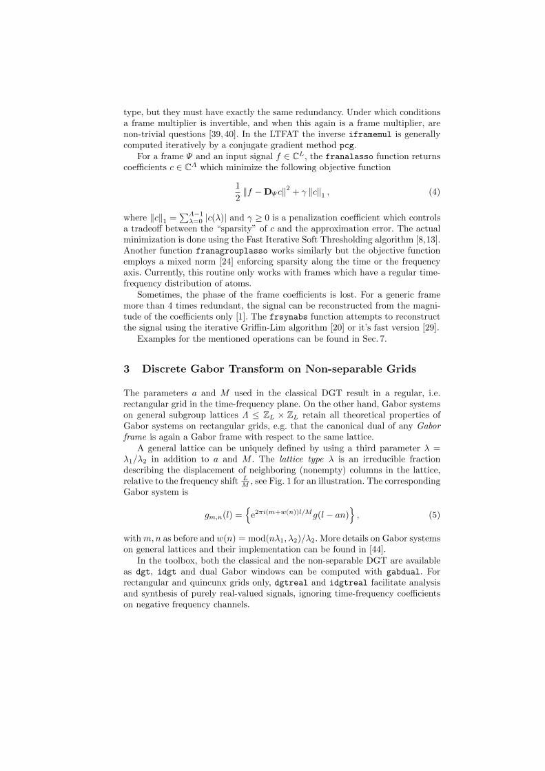
A general lattice can be uniquely defined by using a third parameter λ =λ1/λ2 in addition to a and M . The lattice type λ is an irreducible fractiondescribing the displacement of neighboring (nonempty) columns in the lattice,relative to the frequency shift L
M , see Fig. 1 for an illustration. The correspondingGabor system is
gm,n(l) ={
e2πi(m+w(n))l/Mg(l − an)}, (5)
withm,n as before and w(n) = mod(nλ1, λ2)/λ2. More details on Gabor systemson general lattices and their implementation can be found in [44].
In the toolbox, both the classical and the non-separable DGT are availableas dgt, idgt and dual Gabor windows can be computed with gabdual. Forrectangular and quincunx grids only, dgtreal and idgtreal facilitate analysisand synthesis of purely real-valued signals, ignoring time-frequency coefficientson negative frequency channels.
0 5 10 15 20 25 30 35
0
5
10
15
20
25
30
35
Time / samples
Freq
uenc
y/s
ampl
es
(a) λ1/λ2 = 0
0 5 10 15 20 25 30 35
0
5
10
15
20
25
30
35
Time / samples
Freq
uenc
y/s
ampl
es
(b) λ1/λ2 = 1/2
0 5 10 15 20 25 30 35
0
5
10
15
20
25
30
35
Time / samples
Freq
uenc
y/s
ampl
es
(c) λ1/λ2 = 1/3
0 5 10 15 20 25 30 35
0
5
10
15
20
25
30
35
(d) λ1/λ2 = 2/3
Fig. 1. The figure shows the placement of the Gabor atoms for four different latticetypes in the time-frequency plane. The displayed Gabor system has parameters a = 6,M = 6 and L = 36. The lattice (a) is called rectangular or separable and the lattice (b)is known as the quincunx lattice.
4 Nonstationary Discrete Gabor Transform andFilterbanks
The nonstationary Gabor transform (NSGT) theory [5] generalizes the classicalGabor theory, where the window g, the time step a and the number of frequencychannels M are fixed; to systems with evolving properties over either time orfrequency. A central result of [5] is the definition of conditions on the windowproperties which result in painless nonstationary Gabor frames which admit anefficient computation of the canonical dual system with the same structure. Inthis setup, the frame operator is diagonal and its inversion is a simple operation.In the non-painless case, reconstruction is still possible, assuming the system isa frame, but computation of the dual system is not straightforward and it mightnot retain the original structure.
The painless conditions can be applied either in time or in frequency domain.To avoid confusion, both cases will be shown separately.
4.1 Changing Resolution over Time
Instead of a single window with the fixed time step a, assume a set of N win-dows {gn}n∈{0,...,N−1}, with gn centered around the origin and considering Mn
frequency channels. The resulting discrete nonstationary Gabor system is givenby
gm,n(l) ={
e2πi(l−an)m/Mngn(l − an)}, (6)
for n ∈ {0, . . . , N − 1} ,m ∈ {0, . . . ,Mn − 1} and l ∈ {0, . . . , L− 1}. In contrastto (2) the complex exponentials shift along with the windows due to the (l−an)term. This phase locked convention was chosen to simplify the impementation.The system is painless given the following conditions are satisfied:
1. Each of the windows gn is compactly supported with support length beingless or equal to Mn. This means that the windows have nonzero values onlyin some area around the time position.
2. The adjacent windows overlap so that 0 < A ≤∑N−1n=0 |gn(l − an)|2 ≤ B <
∞, for some positive A and B, for all l ∈ {0, . . . , L− 1}.
Such systems can be designed to adapt the frequency resolution over timein order to better capture characteristics of an analyzed signal and still provideperfect reconstruction. The NSGT in this setting is implemented in the toolboxas nsdgt, its inverse as insdgt.
4.2 Changing Resolution over Frequency
Exploiting the duality in time and frequency domains, we assume M compactlysupported windows {gm}m∈{0,...,M−1} in the frequency domain centered around
frequency 0. Again, if the frequency support of each gm is less or equal to Nmand if the windows overlap sufficiently and cover the whole frequency spectrum,the collection
gm,n(l) ={
e−2πiln/Nm gm(l − bm)}, (7)
for m ∈ {0, . . . ,M − 1}, n ∈ {0, . . . , Nm − 1} and l ∈ {0, . . . , L− 1} defines theDFT of painless nonstationary Gabor system atoms. An alternative interpreta-tion of this result is that {gm} are band-limited frequency responses of filters in aperfect reconstruction filterbank and each of them is followed by a subsamplingoperation with a possibly non-integer factor am = L
Nm. In digital signal process-
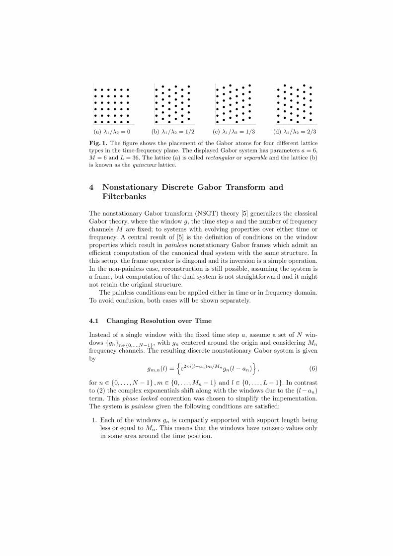
ing terms, the analysis filterbank does not introduce aliasing in subbands, andtherefore no aliasing cancellation property of the synthesis filterbank is needed.This construction proved to be very useful, because it allows designing perfectreconstruction filterbanks with frequency bands adapted to a specific needs, e.g.the constant-Q Transform (CQT) in [5]. The filters in a CQT are placed alongthe frequency axis with a constant ratio of center frequency to bandwidth, or Q-factor. This transform is particularly interesting for an acoustic signal processingbecause it can be tuned to mimic the musical scale allowing to choose the octaveresolution (number of filters per octave). An example of a CQT spectrogram isin Fig. 2 on the left.
Another application of the frequency adapted NSGT is the ERBlet trans-form [27] in which the filters are tuned to mimic the psychoacoustic ERB scale(erblett). An example of the ERBlet spectrogram is in Fig. 2 on the right.
In the toolbox, the frequency adapted nonstationary Gabor systems are im-plemented in the context of the more general filterbank and ifilterbank
routines.
4.3 Uniform Nonstationary Gabor Systems
Nonstationary Gabor systems are uniform if Mn = const. or am = const. in thetime and frequency adapted settings respectively. Such systems admit anotherway of computing the canonical dual systems by inverting a polyphase framematrix [9]. Internally, the toolbox favors the painless algorithm over the uniformone if both are suitable.
Time (s)
Fre
quency (
Hz)
0 0.5 1 1.5 2 0
95.8
187
367
718
1.41e+003
2.75e+003
5.38e+003
1.05e+004
2.21e+004
−50
−40
−30
−20
−10
Time (s)
Fre
qu
en
cy (
Hz)
0 0.5 1 1.5 2 0
100
250
500
1000
2000
4000
8000
16000
−60
−50
−40
−30
−20
Fig. 2. Examples of the CQT spectrogram (left) and the ERBlet spectrogram (right)of an excerpt of the gspi test signal. The figures can be reproduced by runningdemo filterbanks.
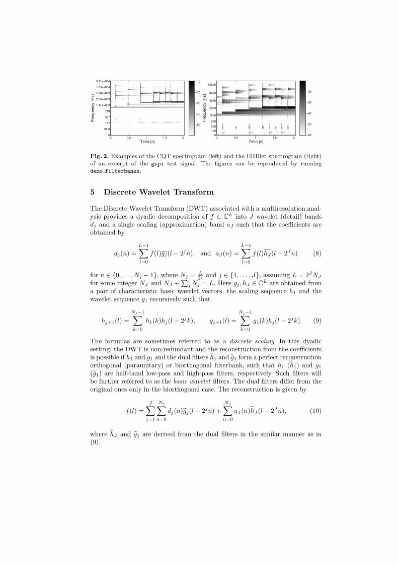
5 Discrete Wavelet Transform
The Discrete Wavelet Transform (DWT) associated with a multiresolution anal-ysis provides a dyadic decomposition of f ∈ CL into J wavelet (detail) bandsdj and a single scaling (approximation) band aJ such that the coefficients areobtained by
dj(n) =
L−1∑l=0
f(l)gj(l − 2jn), and aJ(n) =
L−1∑l=0
f(l)hJ(l − 2Jn) (8)
for n ∈ {0, . . . , Nj − 1}, where Nj = L2j and j ∈ {1, . . . , J}, assuming L = 2JNJ
for some integer NJ and NJ +∑j Nj = L. Here gj , hJ ∈ CL are obtained from
a pair of characteristic basic wavelet vectors, the scaling sequence h1 and thewavelet sequence g1 recursively such that
hj+1(l) =
Nj−1∑k=0
h1(k)hj(l − 2jk), gj+1(l) =
Nj−1∑k=0
g1(k)hj(l − 2jk). (9)
The formulas are sometimes referred to as a discrete scaling. In this dyadicsetting, the DWT is non-redundant and the reconstruction from the coefficientsis possible if h1 and g1 and the dual filters h1 and g1 form a perfect reconstructionorthogonal (paraunitary) or biorthogonal filterbank, such that h1 (h1) and g1(g1) are half-band low-pass and high-pass filters, respectively. Such filters willbe further referred to as the basic wavelet filters. The dual filters differ from theoriginal ones only in the biorthogonal case. The reconstruction is given by
f(l) =
J∑j=1
Nj∑n=0
dj(n)gj(l − 2jn) +
NJ∑n=0
aJ(n)hJ(l − 2Jn), (10)
where hJ and gj are derived from the dual filters in the similar manner as in(9).
The commonly used basic wavelet filters are short FIR filters with smoothand slowly decaying frequency responses. This fact exhibits in a poor frequencyselectivity. Combined with the octave-only frequency division coming from thedyadic structure, this makes the DWT seemingly not attractive from the audiosignal processing point of view. Nevertheless, the DWT was used in a numberof applications dealing with audio signals see e.g. the literature survey in [26].Moreover, there is a body of wavelet filterbank-based transforms improving uponthe DWT properties which are described in the rest of this section.
Fast Wavelet Transform – Mallat’s algorithm (fwt, ifwt): The equations (9)are in fact an enabling factor for the well-known Mallat’s algorithm (also knownas the fast wavelet transform). The algorithm comprises of an iterative appli-cation of the involuted (time reversed and conjugated) elementary two-channelfilterbank followed by subsampling by a factor of two
dj+1 = (aj ∗ g1(.− l))↓2 , aj+1 =(aj ∗ h1(.− l)
)↓2 , (11)
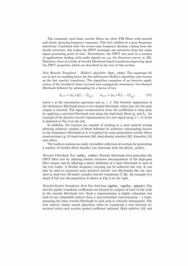
where ∗ is the convolution operation and a0 = f . The iterative application ofthe elementary filterbank forms a tree-shaped filterbank, where just the low-passoutput is iterated. The signal reconstruction from the coefficients is then doneby applying a mirrored filterbank tree using the dual basic filters g1 and h1. Anexample of the discrete wavelet representation of a test signal using J = 11 levelsis depicted in Fig. 3 on the left.
In addition, the routines are capable of working in a more general settingallowing arbitrary number of filters followed by arbitrary subsampling factorsin the elementary filterbank as it is required by some generalized wavelet filtersconstructions e.g.M -band wavelets [38], dual-density wavelets [35], framelets [14]and others.
The toolbox contains an easily extendible collection of routines for generatinga number of wavelet filters families (see functions with the wfilt_ prefix).
Wavelet Filterbank Tree (wfbt, iwfbt): Wavelet filterbank trees generalize theDWT filter tree by allowing further recursive decomposition of the high-passfilter output and by allowing a direct definition of a basic filterbank in each ofthe tree nodes. A flexible frequency covering can be achieved this way. It canalso be used to construct more involved wavelet tree filterbanks like the onesused in dual-tree (M-band) complex wavelet transforms [7,36]. An example of adepth 8 full tree decomposition is shown in Fig. 3 on the right.
Wavelet Packet Transform, Best Tree Selection (wpfbt, iwpfbt, wpbest): Thewavelet packet transform coefficients are formed by outputs of each of the nodein the wavelet filterbank tree. Such a representation is highly redundant butleafs of any admissible subtree form a non-redundant representation – a basis,assuming the basic wavelet filterbank in each node is critically subsampled. Thebest subtree (basis) search algorithm relies on comparing a cost function as-sociated witch each wavelet packet coefficient subband. Both additive [43] and
Time (s)
Subbands
0 0.5 1 1.5 2
a11d11d10
d9d8d7d6d5d4d3d2d1
−40
−30
−20
−10
0
Time (s)
Channel N
o.
0 0.5 1 1.5 2
50
100
150
200
250
−40
−30
−20
−10
0
Fig. 3. On the left, the amplitude of DWT of an excerpt of the gspi test signal usingJ = 11 levels and the 16tap symlet basic wavelet filters (see help for wfilt sym)is displayed. On the right, there is a representation obtained by a depth 8 full treedecomposition. Both representations are non-redundant. The figures can be reproducedby running demo wavelets.
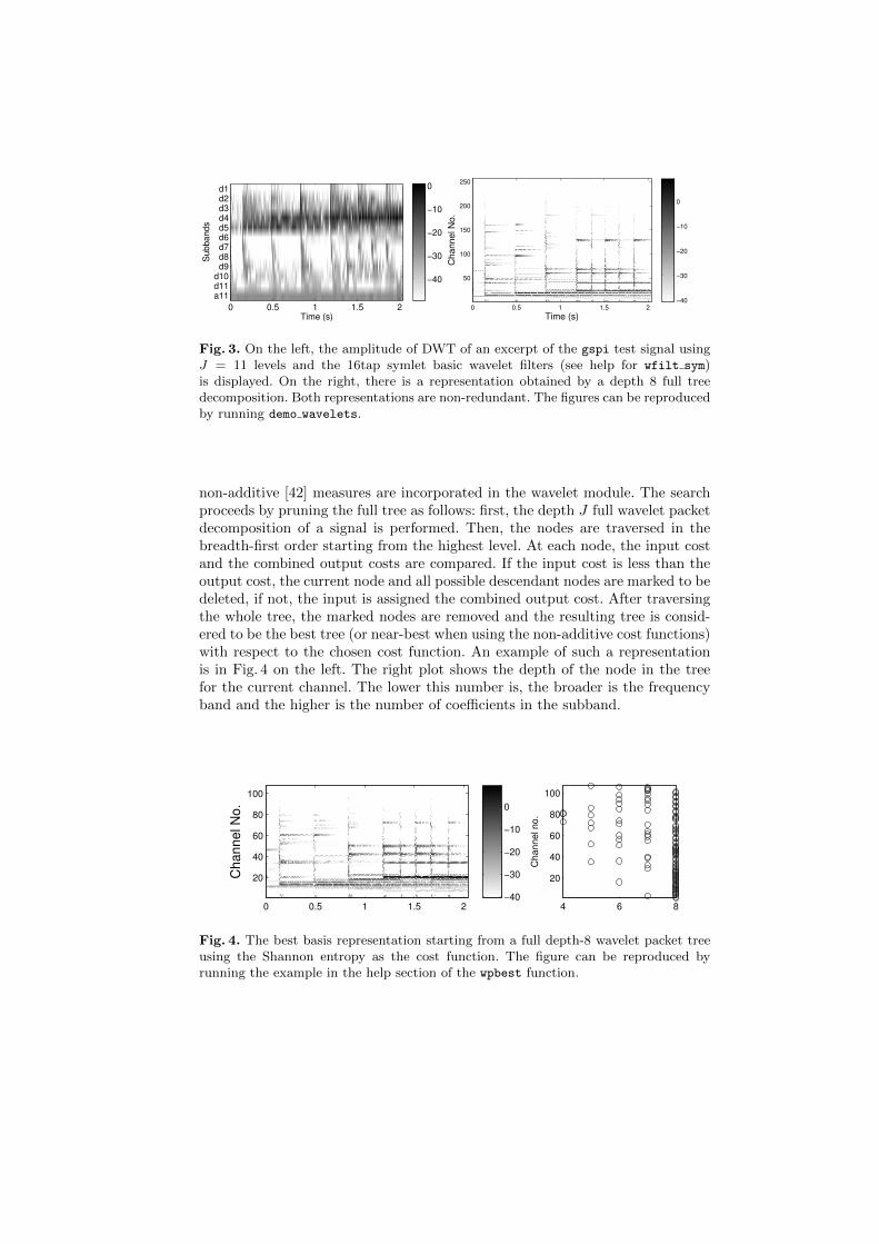
non-additive [42] measures are incorporated in the wavelet module. The searchproceeds by pruning the full tree as follows: first, the depth J full wavelet packetdecomposition of a signal is performed. Then, the nodes are traversed in thebreadth-first order starting from the highest level. At each node, the input costand the combined output costs are compared. If the input cost is less than theoutput cost, the current node and all possible descendant nodes are marked to bedeleted, if not, the input is assigned the combined output cost. After traversingthe whole tree, the marked nodes are removed and the resulting tree is consid-ered to be the best tree (or near-best when using the non-additive cost functions)with respect to the chosen cost function. An example of such a representationis in Fig. 4 on the left. The right plot shows the depth of the node in the treefor the current channel. The lower this number is, the broader is the frequencyband and the higher is the number of coefficients in the subband.
Time (s)
Ch
an
ne
l N
o.
0 0.5 1 1.5 2
20
40
60
80
100
20
40
60
80
100
4 6 8
Channel no.
Depth in the tree.
−40
−30
−20
−10
0
Fig. 4. The best basis representation starting from a full depth-8 wavelet packet treeusing the Shannon entropy as the cost function. The figure can be reproduced byrunning the example in the help section of the wpbest function.
There have been several attempts to use wavelet filterbank trees and waveletpackets to process audio signals, mainly in the context of audio compression.The authors of [25] used M-band wavelet filterbanks in order to divide the fre-quency band into nonlinear frequency bands reminiscent of the tempered musi-cal frequency scale or into an auditory frequency scale. See demo_wfbt from thetoolbox.
All wavelet-type transformations mentioned so far are also available in undec-imated versions in the toolbox (undecimated is sometimes referred to as station-ary in the literature). These representations are very redundant, shift-invariantand the subbands are aliasing-free. The lack of aliasing makes the reconstructionmore robust against coefficient modifications. A fast A-trous algorithm [23] isused when computing such transforms.
There are several boundary extension techniques available for wavelet basedfilterbanks implemented in the toolbox. Apart from the default periodic exten-sion, the toolbox supports two types of symmetric extension and extension withzeros, which might lessen the effect of boundary conditions in some situations.Since the wavelet filters are exclusively short FIR filters, the information aboutthe necessary samples beyond the boundaries can be stored in additional coeffi-cients. The downside of this algorithmic approach is that the underlying frameabstraction becomes unclear.
6 Generalized Fourier Transform
The Generalized Goertzel algorithm (gga): The traditional Goertzel algorithm[19] (introduced in 1958) is a fast algorithm for evaluating individual samples ofthe DFT of f ∈ CL i.e.
c(k) =
L−1∑l=0
f(l)e−2πikl/L . (12)
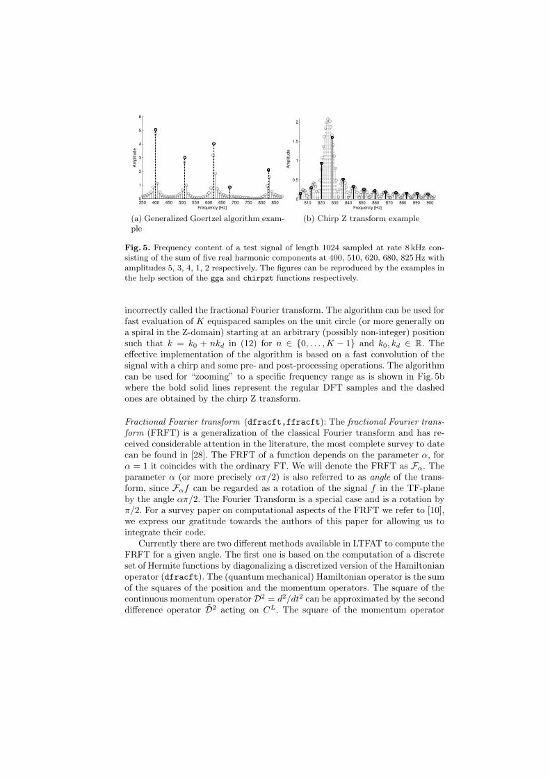
The number of real floating point operations required by the Goertzel algo-rithm is approximately three-quarters of the operations used in the direct evalu-ation. The Goertzel algorithm also does not require explicit evaluation of all thecomplex exponentials. A generalization of the Goertzel algorithm was presentedin [41]. It allows obtaining individual values at an arbitrary position on the unitcircle such that k in (12) does not have to be an integer, with no increase of thecomputational complexity. The algorithm can be useful for detecting the pres-ence of harmonic signals with frequencies not being multiples of the fundamentalfrequency. An example in Fig. 5a shows regular DFT samples (solid lines) of atest signal consisting of a sum of harmonic components and samples obtainedby the generalized Goertzel algorithm (bold dashed lines) selecting k to coincidewith the known frequencies.
The chirp Z transform (chirpzt): The toolbox also contains an implementationof a similar purpose algorithm called the chirp Z transform [34], sometimes
350 400 450 500 550 600 650 700 750 800 8500
1
2
3
4
5
6
Frequency [Hz]
Am
plit
ude
(a) Generalized Goertzel algorithm exam-ple
810 820 830 840 850 860 870 880 890 9000
0.5
1
1.5
2
Frequency [Hz]
Am
plit
ude
(b) Chirp Z transform example
Fig. 5. Frequency content of a test signal of length 1024 sampled at rate 8 kHz con-sisting of the sum of five real harmonic components at 400, 510, 620, 680, 825 Hz withamplitudes 5, 3, 4, 1, 2 respectively. The figures can be reproduced by the examples inthe help section of the gga and chirpzt functions respectively.
incorrectly called the fractional Fourier transform. The algorithm can be used forfast evaluation of K equispaced samples on the unit circle (or more generally ona spiral in the Z-domain) starting at an arbitrary (possibly non-integer) positionsuch that k = k0 + nkd in (12) for n ∈ {0, . . . ,K − 1} and k0, kd ∈ R. Theeffective implementation of the algorithm is based on a fast convolution of thesignal with a chirp and some pre- and post-processing operations. The algorithmcan be used for “zooming” to a specific frequency range as is shown in Fig. 5bwhere the bold solid lines represent the regular DFT samples and the dashedones are obtained by the chirp Z transform.
Fractional Fourier transform (dfracft,ffracft): The fractional Fourier trans-form (FRFT) is a generalization of the classical Fourier transform and has re-ceived considerable attention in the literature, the most complete survey to datecan be found in [28]. The FRFT of a function depends on the parameter α, forα = 1 it coincides with the ordinary FT. We will denote the FRFT as Fα. Theparameter α (or more precisely απ/2) is also referred to as angle of the trans-form, since Fαf can be regarded as a rotation of the signal f in the TF-planeby the angle απ/2. The Fourier Transform is a special case and is a rotation byπ/2. For a survey paper on computational aspects of the FRFT we refer to [10],we express our gratitude towards the authors of this paper for allowing us tointegrate their code.
Currently there are two different methods available in LTFAT to compute theFRFT for a given angle. The first one is based on the computation of a discreteset of Hermite functions by diagonalizing a discretized version of the Hamiltonianoperator (dfracft). The (quantum mechanical) Hamiltonian operator is the sumof the squares of the position and the momentum operators. The square of thecontinuous momentum operator D2 = d2/dt2 can be approximated by the seconddifference operator D2 acting on CL. The square of the momentum operator
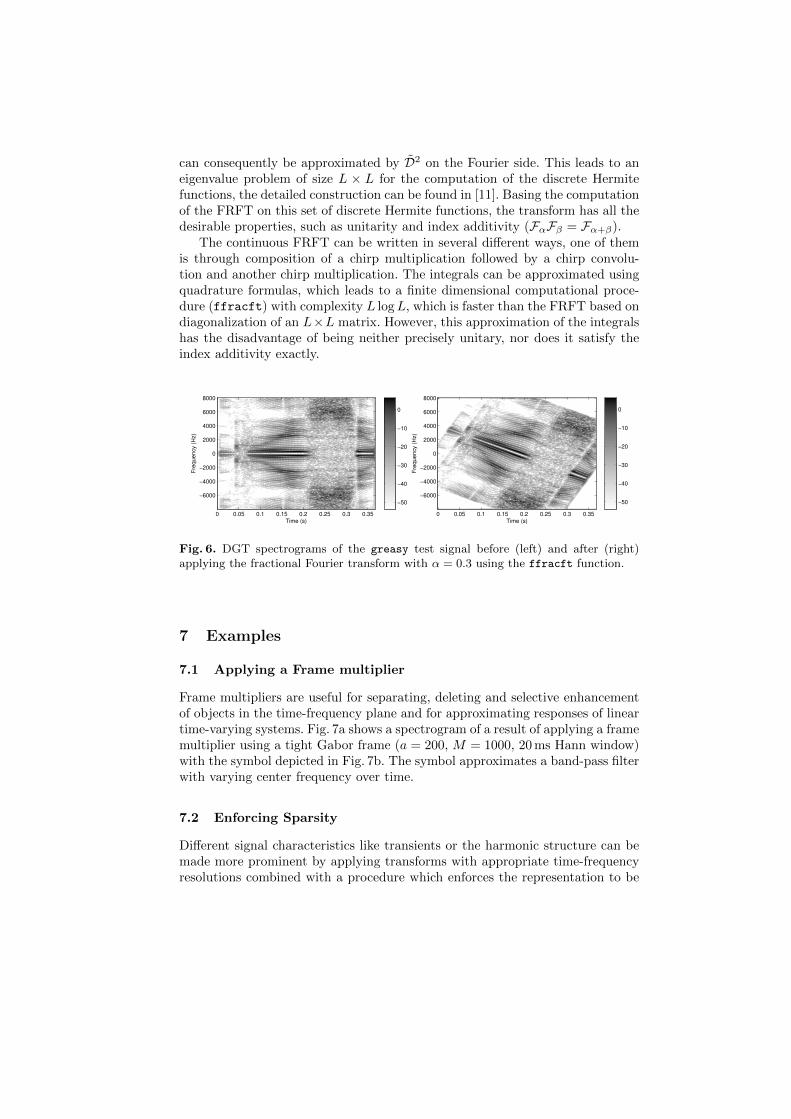
can consequently be approximated by D2 on the Fourier side. This leads to aneigenvalue problem of size L × L for the computation of the discrete Hermitefunctions, the detailed construction can be found in [11]. Basing the computationof the FRFT on this set of discrete Hermite functions, the transform has all thedesirable properties, such as unitarity and index additivity (FαFβ = Fα+β).
The continuous FRFT can be written in several different ways, one of themis through composition of a chirp multiplication followed by a chirp convolu-tion and another chirp multiplication. The integrals can be approximated usingquadrature formulas, which leads to a finite dimensional computational proce-dure (ffracft) with complexity L logL, which is faster than the FRFT based ondiagonalization of an L×L matrix. However, this approximation of the integralshas the disadvantage of being neither precisely unitary, nor does it satisfy theindex additivity exactly.
Time (s)
Fre
qu
en
cy (
Hz)
0 0.05 0.1 0.15 0.2 0.25 0.3 0.35
−6000
−4000
−2000
0
2000
4000
6000
8000
−50
−40
−30
−20
−10
0
Time (s)
Fre
qu
en
cy (
Hz)
0 0.05 0.1 0.15 0.2 0.25 0.3 0.35
−6000
−4000
−2000
0
2000
4000
6000
8000
−50
−40
−30
−20
−10
0
Fig. 6. DGT spectrograms of the greasy test signal before (left) and after (right)applying the fractional Fourier transform with α = 0.3 using the ffracft function.
7 Examples
7.1 Applying a Frame multiplier
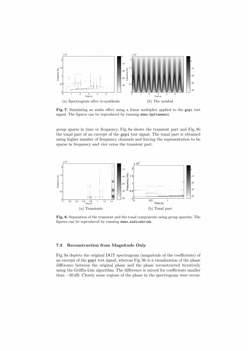
Frame multipliers are useful for separating, deleting and selective enhancementof objects in the time-frequency plane and for approximating responses of lineartime-varying systems. Fig. 7a shows a spectrogram of a result of applying a framemultiplier using a tight Gabor frame (a = 200, M = 1000, 20 ms Hann window)with the symbol depicted in Fig. 7b. The symbol approximates a band-pass filterwith varying center frequency over time.
7.2 Enforcing Sparsity
Different signal characteristics like transients or the harmonic structure can bemade more prominent by applying transforms with appropriate time-frequencyresolutions combined with a procedure which enforces the representation to be
Time (s)
Fre
quency (
Hz)
0 1 2 3 4 50
0.5
1
1.5
2
x 104
−40
−30
−20
−10
0
(a) Spectrogram after re-synthesis
Time (s)
Fre
quency (
Hz)
0 1 2 3 4 50
0.5
1
1.5
2
x 104
−40
−30
−20
−10
0
(b) The symbol
Fig. 7. Simulating an audio effect using a frame multiplier applied to the gspi testsignal. The figures can be reproduced by running demo bpframemul.
group sparse in time or frequency. Fig. 8a shows the transient part and Fig. 8bthe tonal part of an excerpt of the gspi test signal. The tonal part is obtainedusing higher number of frequency channels and forcing the representation to besparse in frequency and vice versa the transient part.
Time (s)
Fre
quen
cy (
Hz)
0 0.2 0.4 0.6 0.8 1 1.2 1.40
0.5
1
1.5
2
x 104
−50
−40
−30
−20
−10
(a) Transients
Time (s)
Fre
qu
en
cy (
Hz)
0 0.5 10
0.5
1
1.5
2
x 104
−40
−30
−20
−10
0
(b) Tonal part
Fig. 8. Separation of the transient and the tonal components using group sparsity. Thefigures can be reproduced by running demo audioshrink.
7.3 Reconstruction from Magnitude Only
Fig. 9a depicts the original DGT spectrogram (magnitude of the coefficients) ofan excerpt of the gspi test signal, whereas Fig. 9b is a visualization of the phasedifference between the original phase and the phase reconstructed iterativelyusing the Griffin-Lim algorithm. The difference is zeroed for coefficients smallerthan −50 dB. Clearly some regions of the phase in the spectrogram were recon-
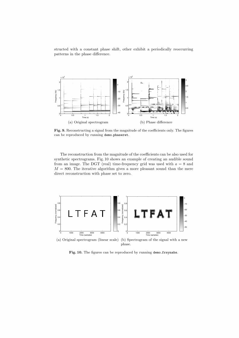
structed with a constant phase shift, other exhibit a periodically reoccurringpatterns in the phase difference.
Time (s)
Fre
quency (
Hz)
0 0.5 1 1.5 20
0.5
1
1.5
2
x 104
−40
−30
−20
−10
0
(a) Original spectrogram
Time (s)
Fre
quency (
Hz)
0 0.5 1 1.5 20
0.5
1
1.5
2
x 104
0.5
1
1.5
2
2.5
3
(b) Phase difference
Fig. 9. Reconstructing a signal from the magnitude of the coefficients only. The figurescan be reproduced by running demo phaseret.
The reconstruction from the magnitude of the coefficients can be also used forsynthetic spectrograms. Fig. 10 shows an example of creating an audible soundfrom an image. The DGT (real) time-frequency grid was used with a = 8 andM = 800. The iterative algorithm gives a more pleasant sound than the meredirect reconstruction with phase set to zero.
Time (samples)
Fre
quency (
norm
aliz
ed)
0 1000 2000 3000 40000
0.2
0.4
0.6
0.8
1
0
0.2
0.4
0.6
0.8
1
(a) Original spectrogram (linear scale)
Time (samples)
Fre
qu
ency (
norm
aliz
ed)
0 1000 2000 3000 40000
0.2
0.4
0.6
0.8
1
−50
−40
−30
−20
−10
0
(b) Spectrogram of the signal with a newphase.
Fig. 10. The figures can be reproduced by running demo frsynabs.
8 Block-stream Processing Framework
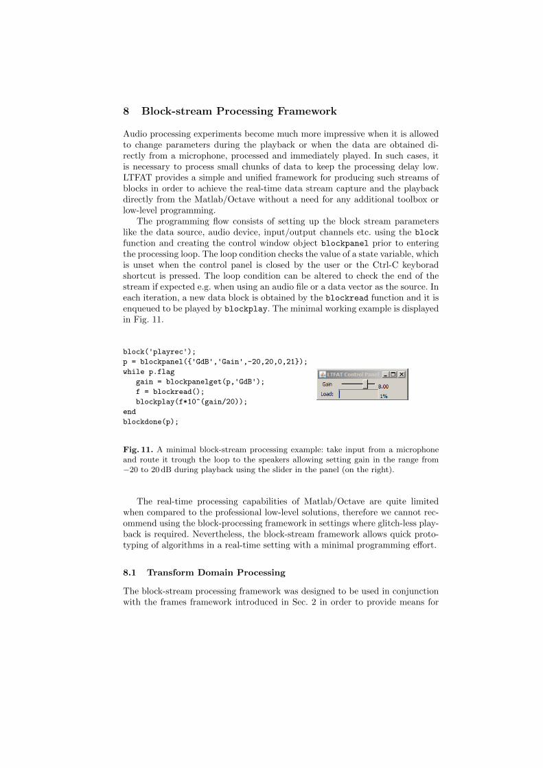
Audio processing experiments become much more impressive when it is allowedto change parameters during the playback or when the data are obtained di-rectly from a microphone, processed and immediately played. In such cases, itis necessary to process small chunks of data to keep the processing delay low.LTFAT provides a simple and unified framework for producing such streams ofblocks in order to achieve the real-time data stream capture and the playbackdirectly from the Matlab/Octave without a need for any additional toolbox orlow-level programming.
The programming flow consists of setting up the block stream parameterslike the data source, audio device, input/output channels etc. using the block
function and creating the control window object blockpanel prior to enteringthe processing loop. The loop condition checks the value of a state variable, whichis unset when the control panel is closed by the user or the Ctrl-C keyboradshortcut is pressed. The loop condition can be altered to check the end of thestream if expected e.g. when using an audio file or a data vector as the source. Ineach iteration, a new data block is obtained by the blockread function and it isenqueued to be played by blockplay. The minimal working example is displayedin Fig. 11.
block('playrec');
p = blockpanel({'GdB','Gain',-20,20,0,21});
while p.flag
gain = blockpanelget(p,'GdB');
f = blockread();
blockplay(f*10^(gain/20));
end
blockdone(p);
Fig. 11. A minimal block-stream processing example: take input from a microphoneand route it trough the loop to the speakers allowing setting gain in the range from−20 to 20 dB during playback using the slider in the panel (on the right).
The real-time processing capabilities of Matlab/Octave are quite limitedwhen compared to the professional low-level solutions, therefore we cannot rec-ommend using the block-processing framework in settings where glitch-less play-back is required. Nevertheless, the block-stream framework allows quick proto-typing of algorithms in a real-time setting with a minimal programming effort.
8.1 Transform Domain Processing
The block-stream processing framework was designed to be used in conjunctionwith the frames framework introduced in Sec. 2 in order to provide means for
a real-time time-frequency analysis, visualization, modification and synthesis.There are two obstacles when considering applying transforms from the toolboxon a real-time stream of data blocks:
1. The computational complexity of the desired operation.2. The processed signal periodicity assumption.
The fast execution is achieved by pre-computing all the fixed data by meansof the blockframeaccel or blockframepairacel functions prior entering theprocessing loop complemented with an efficient C implementation of algorithms.The periodicity assumption goes against the way how data are actually obtainedin a real-time setting. Therefore the direct naive application of the transform toindividual blocks will produce “bad” coefficients not fit to be directly manipu-lated or plotted even though the block can be reconstructed perfectly. LTFATsupports two approaches for adapting the transforms to avoid or at least lessenthe impact of the assumed periodicity: the combined overlap-save/overlap-addapproach for transforms using FIR windows/filters and the slicing window ap-proach for all other transforms.
a) The combined overlap-save/overlap-add approach is conceptually similar tothe one in [33], where it was used for developing an algorithm for an error-freeblock-wise discrete wavelet transform. The algorithm is based on a principle ofoverlap-save (also known as the overlap-discard) type block convolution for theanalysis and overlap-add type block convolution for the synthesis. The necessaryoverlap lengths can be determined exactly from the finite windows/filter lengthsthe transform is based on.
The algorithm as described here holds for the following assumptions:
1. The window hop size a (or the subsampling factor) is uniform for all windows.2. The window length is Lw = k2a + 1 for k being some positive integer and
the origin is at the middle sample.3. The blocks have uniform lengths Lb = la for l being some positive integer.4. Lb > Lw.
These assumptions are often too restrictive in practice, but more general settingsrequire rather large number of additional operations the description of wouldobscure the principal idea of the algorithm. The current implementation requiresthe first assumption and uniform length (though arbitrary) FIR windows havingthe same position of the origin. Moreover, the implementation is able to handleblocks with varying lengths.
Analysis part:
1. Read a block of data, extend it from the left side by the Lw− 1 last samplesform the previous block.
2. Apply the transform to the extended block.3. From the resulting coefficients, keep only those at indexes {k, . . . , l + k − 1}
starting counting from zero.
The last step discards coefficients which are time-aliased due to the implicitperiodic boundary handling. The discarding is done from the both sides becausethe windows used in the LTFAT computation routines are not causal. The re-maining coefficients are equal to the corresponding coefficients from a transformof a signal without dividing it into blocks. The cropped coefficients, possiblymodified, form the input for the synthesis part of the algorithm.
Synthesis part:
1. Create zero arrays of length 2k+ l for each channel and copy the coefficientsobtained by the analysis procedure to time positions {k, . . . , l + k − 1}.
2. Apply the inverse transformation to the extended coefficients.3. Recall the Lw− 1 last samples from the previous block and add them to the
first Lw − 1 samples of the current block.4. Store the last Lw − 1 samples as the overlap used in the next block.
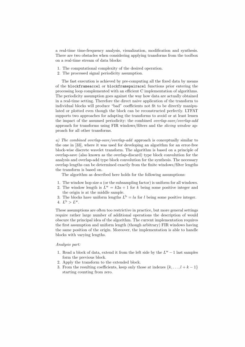
A toy example of applying the algorithm is depicted in Fig. 12 and Fig. 13for the analysis and synthesis parts respectively.
f
c
c0
c1
c2
f0
f1
f2
zeros
0 9 18
0 1 2 3 4
0 1 2 3 4
0 1 2 3 4
Fig. 12. An example of the analysis part of the combined overlap-save/overlap-addalgorithm for a = 3, Lb = 9 and Lw = 7 (l = 3, k = 1). The figure shows the first threeblocks of the signal f and the true time positions of coefficients c. Each of the blocks f0,f1 and f2 is extended from the left side by Lw − 1 = 6 samples and transformed. Therespective coefficients c0, c1, c2 are obtained and only the ones with indexes {1, 2, 3}are retained. Note the algorithm produces k additional coefficients at the beginningwhen compared to the true coefficients c.
b) The Slicing window method was originally presented in [22]. In contrast tothe previous approach, the slicing window method does not try to determineoverlaps exactly, but instead employs a slicing window to weigh blocks of samplesproducing slices. After windowing, the slice is optionally symmetrically zero-padded to lessen the effect of the time aliasing. After reconstruction, the sliceis weighted by a dual slicing window and the reconstructed signal assembled in
c1
f1
f0
f2
f
0 0
0 0
0 0c2
c3
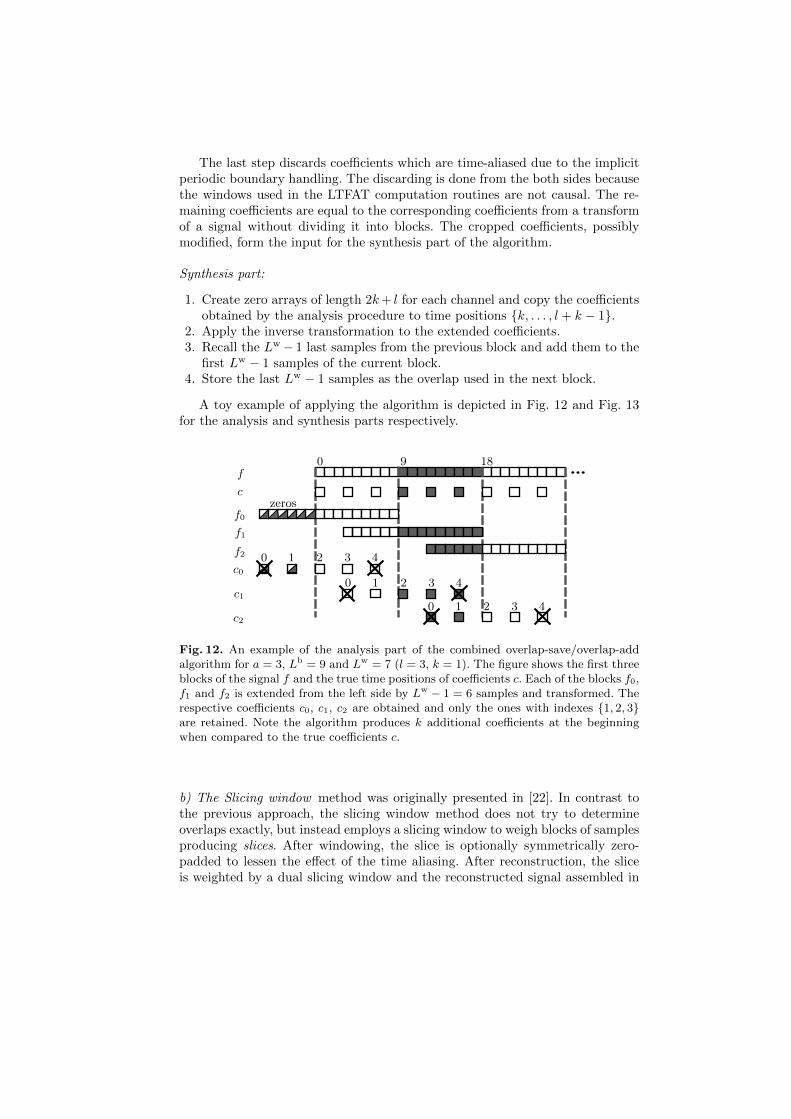
Fig. 13. An example of the synthesis part of the combined overlap-save/overlap-addalgorithm. The coefficients c0,c1 and c2 are extended with zeros and the reconstructedblocks f0,f1 and f2 are overlapped. Note the overall delay of the algorithm is Lw−1 = 6samples.
an overlap-add manner. The same slicing window can be used for dividing thesignal and for the assembly, if the squares of all it’s time shifts form a partitionof unity. More general combinations of windows are also possible, see [22] forthe details. Note that the coefficients reflect the shape of the slicing window, sonon-linear processing like thresholding applied directly to the coefficients mayintroduce blocking artifacts. In the toolbox, the method is implemented in sucha way the slicing window is applied to a concatenation of the previous and thecurrent block so the slicing window shift is Lb effectively. By default, a square-root of a peak-normalized Hann window is used but the programming interfaceallows specifying customized slicing windows.
In the toolbox, the demos with the demo blockproc prefix show the block-stream processing framework in action. Fig. 14 is a screenshot of one of the demosdoing a real-time visualization of the discrete Gabor transform spectrogram ofthe gspi test signal played in the loop. The coefficients are obtained using a FIRwindow and the analysis part of the combined overlap-save/overlap-add method.Another demo plots a real-time CQT spectrogram. The same test signal is usedin the screenshot in Fig. 15. The coefficients are obtained by the slicing windowmethod.
9 Design and Implementation
The toolbox is designed in such a way that the functions forming the program-ming interface in most cases only check and format the user defined inputs andpass them further to the routines with the comp prefix, that perform the actualcomputations. The majority of the comp functions can be replaced (shadowed)by compiling the MEX/OCT files with the identical name to speedup the com-putations. The MEX/OCT files themselves do not contain the computations,but again just format the inputs (unify data types, change complex numbers
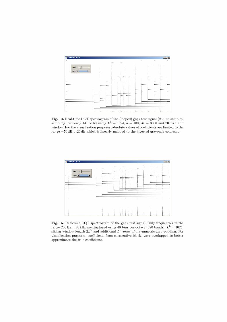
Fig. 14. Real-time DGT spectrogram of the (looped) gspi test signal (262144 samples,sampling frequency 44.1 kHz) using Lb = 1024, a = 100, M = 3000 and 20 ms Hannwindow. For the visualization purposes, absolute values of coefficients are limited to therange −70 dB. . . 20 dB which is linearly mapped to the inverted grayscale colormap.
Fig. 15. Real-time CQT spectrogram of the gspi test signal. Only frequencies in therange 200 Hz. . . 20 kHz are displayed using 48 bins per octave (320 bands), Lb = 1024,slicing window length 2Lb and additional Lb zeros of a symmetric zero padding. Forvisualization purposes, coefficients from consecutive blocks were overlapped to betterapproximate the true coefficients.
memory layout) and obtain data pointers and call the actual computationalroutine(s) from the separately compiled backend C library to which they linkto. The backend library depends on the FFTW library and on the BLAS andLAPACK libraries, which are usually already contained in the Matlab/Octaveinstallation. On Windows systems, a manual installation of the FFTW libraryis necessary at the moment when using Matlab. In order to minimize the coderepetition, the backend library is built in such a way the actual code is indepen-dent of the desired data type (floating data types with different precision) andeven of the real or the complex data type where possible.
The regular toolbox functionality can be used without the backend libraryand MEX/OCT interfaces. The block-stream processing framework howeverrequires compiling the MEX interface playrec (http://www.playrec.co.uk,contained in LTFAT), which depends on the Portaudio library (http://www.portaudio.com), which is again distributed with recent versions of Matlab. Thecompilation process is automated via the ltfatmex command, but pre-builtpackages can be downloaded from the toolbox webpage. An additional possibil-ity for Octave users is installing LTFAT directly trough the integrated packagemanagement system pkg, which takes care of compiling everything during theinstallation process.
10 Outlook
This section describes possible enhancements and features of the toolbox whichmight be included in the future versions.
Quadratic time-frequency distributions – Although the family of quadratic time-frequency distributions cannot be associated with frames because of their non-linear character, they offer yet another way of studying audio signal features [12].Moreover, algorithms for synthesizing signals from their quadratic representa-tions exist, so there is a possibility for doing modifications on the coefficients ina similar manner as with frame multipliers.
Modern algorithms for phase-less reconstruction – A reconstruction from onlythe magnitude of frame coefficients is currently a very active topic in research. Weplan to implement some of the modern algorithms, see e.g. [15], to complementthe Griffin-Lim algorithm.
Gabor dual windows using convex optimization – Explicit formulas for Gabordual windows are known only for the canonical dual frame. If the frame systemis redundant, infinitely many dual windows exists. Using results from [30,31] wewill add an option to search for the optimal dual window given a prior criterion.
Algorithms for computation of optimal dual uniform FIR filterbank frames –The current algorithm for computing dual uniform FIR filterbank (based on [9])frames in LTFAT suffers from two drawbacks. First, it is capable of computing
the canonical dual frame only and it does not preserve the FIR property. Theplan is to include results from [18] to allow more freedom in choosing the optimalFIR filterbank dual frames.
Acknowledgments. The authors would like to thank the people that made con-tributions to the toolbox: Remi Decorsiere, Monika Dorfler, Nina Engelputzeder,Hans Feichtinger, Thomas Hrycak, Florent Jaillet, A.J.E.M. Janssen, NorbertKaiblinger, Matthieu Kowalski, Ewa Matusiak, Piotr Majdak, Nathanael Per-raudin, Pavel Rajmic, Thomas Strohmer, Bruno Torresani, Jordy van Velthovenand Tobias Werther.
We would like to express our gratitude towards authors of the Uvi Wavetoolbox [32], from which we have taken some wavelet filters generation routines.
The work on this paper was partly supported by the Austrian Science Fund(FWF) START-project FLAME (’Frames and Linear Operators for AcousticalModeling and Parameter Estimation’; Y 551-N13).
References
1. Balan, R., Casazza, P., Edidin, D.: On signal reconstruction without phase. Appl.Comput. Harmon. Anal. 20(3), 345–356 (2006)
2. Balazs, P.: Frames and finite dimensionality: Frame transformation, classificationand algorithms. Applied Mathematical Sciences 2(41–44), 2131–2144 (2008)
3. Balazs, P., Dorfler, M., Kowalski, M., Torresani, B.: Adapted and adaptive lineartime-frequency representations: a synthesis point of view. IEEE Signal ProcessingMagazine (special issue: Time-Frequency Analysis and Applications) 30(6), 20–31(2013)
4. Balazs, P.: Basic definition and properties of Bessel multipliers. Journal of Math-ematical Analysis and Applications 325(1), 571–585 (January 2007), http://dx.doi.org/10.1016/j.jmaa.2006.02.012
5. Balazs, P., Dorfler, M., Jaillet, F., Holighaus, N., Velasco, G.A.: Theory, im-plementation and applications of nonstationary Gabor frames. J. Comput.Appl. Math. 236(6), 1481–1496 (2011), http://ltfat.sourceforge.net/notes/
ltfatnote018.pdf
6. Balazs, P., Feichtinger, H.G., Hampejs, M., Kracher, G.: Double preconditioningfor Gabor frames. IEEE Trans. Signal Process. 54(12), 4597–4610 (December 2006),http://dx.doi.org/10.1109/TSP.2006.882100
7. Bayram, I., Selesnick, I.W.: On the dual-tree complex wavelet packet and M-bandtransforms. Signal Processing, IEEE Transactions on 56(6), 2298–2310 (2008)
8. Beck, A., Teboulle, M.: A fast iterative shrinkage-thresholding algorithm for linearinverse problems. SIAM J. Img. Sci. 2(1), 183–202 (Mar 2009), http://dx.doi.org/10.1137/080716542
9. Bolcskei, H., Hlawatsch, F., Feichtinger, H.G.: Frame-theoretic analysis of over-sampled filter banks. Signal Processing, IEEE Transactions on 46(12), 3256–3268(2002)
10. Bultheel, A., Martınez, S.: Computation of the fractional Fourier transform. Appl.Comput. Harmon. Anal. 16(3), 182–202 (2004)
11. Candan, C., Kutay, M.A., Ozaktas, H.M.: The discrete fractional Fourier trans-form. IEEE Trans. Signal Process. 48(5), 1329–1337 (2000)
12. Cohen, L.: Time-frequency distributions-a review. Proceedings of the IEEE 77(7),941–981 (Jul 1989)
13. Daubechies, I., Defrise, M., De Mol, C.: An iterative thresholding algorithm forlinear inverse problems with a sparsity constraint. Communications in Pure andApplied Mathematics 57, 1413–1457 (2004)
14. Daubechies, I., Han, B., Ron, A., Shen, Z.: Framelets: MRA-based constructionsof wavelet frames. Applied and Computational Harmonic Analysis 14(1), 1 – 46(2003)
15. Decorsiere, R., Søndergaard, P.L., Buchholz, J., Dau, T.: Modulation filtering usingan optimization approach to spectrogram reconstruction. In: Proceedings of ForumAcusticum 2011. European Acoustics Association (2011)
16. Feichtinger, H.G., Strohmer, T. (eds.): Gabor analysis and algorithms. Birkhauser,Boston (1998)
17. Flandrin, P.: Time-frequency/time-scale analysis, Wavelet Analysis and its Appli-cations, vol. 10. Academic Press Inc., San Diego, CA (1999), with a preface byYves Meyer, Translated from the French by Joachim Stockler
18. Gauthier, J., Duval, L., Pesquet, J.: Optimization of synthesis oversampled complexfilter banks. Signal Processing, IEEE Transactions on 57(10), 3827–3843 (Oct 2009)
19. Goertzel, G.: An algorithm for the evaluation of finite trigonometric series. Amer-ican Mathematical Monthly 65(1), 34–35 (1958)
20. Griffin, D., Lim, J.: Signal estimation from modified Short-Time Fourier Trans-form. IEEE Transactions on Acoustics, Speech, and Signal Processing 32(2), 236– 243 (apr 1984)
21. Grochenig, K.: Foundations of Time-Frequency Analysis. Birkhauser (2001)22. Holighaus, N., Dorfler, M., Velasco, G.A., Grill, T.: A framework for invertible, real-
time constant-Q transforms. IEEE Transactions on Audio, Speech and LanguageProcessing 21(4), 775 –785 (2013)
23. Holschneider, M., Kronland-Martinet, R., Morlet, J., Tchamitchian, P.: A real-timealgorithm for signal analysis with the help of the wavelet transform. In: Combes,J.M., Grossmann, A., Tchamitchian, P. (eds.) Wavelets. Time-Frequency Methodsand Phase Space. p. 286 (1989)
24. Kowalski, M.: Sparse regression using mixed norms. Appl. Comput. Harmon. Anal.27(3), 303–324 (2009), http://hal.archives-ouvertes.fr/hal-00202904/
25. Kurth, F., Clausen, M.: Filter bank tree and M-band wavelet packet algorithms inaudio signal processing. Signal Processing, IEEE Transactions on 47(2), 549–554(Feb 1999)
26. Merry, R., Steinbuch, M., van de Molengraft, M.: Wavelet the-ory and applications, A literature study. DCT 2005.53 (2005), URL:http://alexandria.tue.nl/repository/books/612762.pdf
27. Necciari, T., Balazs, P., Holighaus, N., Søndergaard, P.L.: The ERBlet transform:An auditory-based time-frequency representation with perfect reconstruction. In:Proceedings of the 38th International Conference on Acoustics, Speech, and SignalProcessing (ICASSP 2013). pp. 498–502. IEEE, Vancouver, Canada (May 2013)
28. Ozaktas, H.M., Zalevsky, Z., Kutay, M.A.: The fractional Fourier transform. JohnWiley and Sons (2001)
29. Perraudin, N., Balazs, P., Sondergaard, P.: A fast Griffin-Lim algorithm. In: Ap-plications of Signal Processing to Audio and Acoustics (WASPAA), 2013 IEEEWorkshop on. pp. 1–4 (Oct 2013)
30. Perraudin, N., Holighaus, N., Soendergaard, P., Balazs, P.: Gabor dual windowsusing convex optimization. In: Proceeedings of the 10th International Conferenceon Sampling theory and Applications (SAMPTA 2013) (2013)
31. Perraudin, N., Holighaus, N., Søndergaard, P.L., Balazs, P.: Designing gabor win-dows using convex optimization. http://arxiv.org (2014), arXiv:1401.6033
32. Prelcic, N.G., Marquez, O.W., Gonzalez, S.: Uvi Wave, the ultimate toolbox forwavelet transforms and filter banks. In: Proceedings of the Fourth Bayona Work-shop on Intelligent Methods in Signal Processing and Communications. pp. 224–227. Bayona, Spain (1996)
33. Prusa, Z.: Segmentwise Discrete Wavelet Transform. Ph.D. thesis, Brno Universityof Technology, Brno (2012)
34. Rabiner, L., Schafer, R., Rader, C.: The chirp Z-transform algorithm. Audio andElectroacoustics, IEEE Transactions on 17(2), 86–92 (1969)
35. Selesnick, I.W.: The double density DWT. In: Wavelets in Signal and Image Anal-ysis, pp. 39–66. Springer (2001)
36. Selesnick, I.W.: The double-density dual-tree DWT. Signal Processing, IEEETransactions on 52(5), 1304–1314 (2004)
37. Søndergaard, P.L., Torresani, B., Balazs, P.: The Linear Time Frequency AnalysisToolbox. International Journal of Wavelets, Multiresolution Analysis and Informa-tion Processing 10(4) (2012)
38. Steffen, P., Heller, P., Gopinath, R., Burrus, C.: Theory of regular M-band waveletbases. Signal Processing, IEEE Transactions on 41(12), 3497–3511 (Dec 1993)
39. Stoeva, D.T., Balazs, P.: Invertibility of multipliers. Applied and ComputationalHarmonic Analysis 33(2), 292–299 (2012)
40. Stoeva, D.T., Balazs, P.: Canonical forms of unconditionally convergent multipliers.Journal of Mathematical Analysis and Applications 399, 252–259 (2013)
41. Sysel, P., Rajmic, P.: Goertzel algorithm generalized to non-integer multiplesof fundamental frequency. EURASIP Journal on Advances in Signal Processing2012(1), 56 (2012)
42. Taswell, C.: Near-best basis selection algorithms with non-additive informationcost functions. In: Proceedings of the IEEE International Symposium on Time-Frequency and Time-Scale Analysis. pp. 13–16. IEEE Press (1994)
43. Wickerhauser, M.V.: Lectures on wavelet packet algorithms. In: Lecture notes,INRIA (1992)
44. Wiesmeyr, C., Holighaus, N., Søndergaard, P.L.: Efficient algorithms for discreteGabor transforms on a nonseparable lattice. IEEE Trans. Signal Process. 61(20)(2013)