The large mean body size of mammalian herbivores explains ... NatEcolEvol.pdf · The large mean body size of mammalian herbivores explains the productivity paradox during the Last

Articleshttps://doi.org/10.1038/s41559-018-0481-y

© 2018 Macmillan Publishers Limited, part of Springer Nature. All rights reserved.

1Laboratoire des Sciences du Climat et de l’Environnement, LSCE CEA CNRS UVSQ, Gif Sur Yvette, France. 2Sorbonne Universités (UPMC), CNRS-IRD-MNHN, LOCEAN/IPSL, Paris, France. 3CNRS, Université Grenoble Alpes, Institut de Géosciences de l’Environnement (IGE), Grenoble, France. 4Sino-French Institute for Earth System Science, College of Urban and Environmental Sciences, Peking University, Beijing, China. 5CSIC, Global Ecology Unit, CREAF-CSIC, Universitat Autònoma de Barcelona, Bellaterra, Spain. 6Northeast Science Station, Pacific Institute for Geography, Russian Academy of Sciences, Cherskii, Russia. *e-mail: [email protected]

Mammalian herbivores live in all major terrestrial ecosys-tems on Earth1. During the past decades, our understand-ing of the important role that large mammalian herbivores

(body mass > 10 kg)2 have in controlling vegetation structure and carbon and nutrient flows within ecosystems has increased. In herbivore-exclusion experiments, large herbivores have been shown to reduce woody cover3,4, modify the traits and composi-tion of herbaceous species5,6, accelerate nutrient cycling rates7,8, increase grassland primary production9,10 and reduce fire occur-rence11. In palaeoecological studies, the late Pleistocene megafaunal extinctions have been shown to result in cascading effects on veg-etation structure and ecosystem function12, including biome shifts from mixed open woodlands to more uniform, closed forests and increased fire activities13,14.

During the last glacial period from 110 to 14 thousand years before present (kyr bp, taken to be ad 1950), the mammoth steppe ecosystem, also referred to as ‘steppe–tundra’ or ‘tundra–steppe’15, prevailed in Eurasia and North America, covering vast areas that are occupied by boreal forests and tundra today16–20. Characterized by a continental climate, intense aridity and domination of herba-ceous vegetation, including graminoids, forbs and sedges, the mam-moth steppe sustained a high diversity and probably a high density of megafaunal herbivores, such as woolly mammoths, muskoxen, horses and bison19,21–23. However, the main driving force behind the maintenance and disappearance of the mammoth steppe remains controversial. Alternative to the climate hypothesis that attributes the end-Pleistocene vegetation transformation and mammalian

extinctions to climate change, the ‘keystone herbivore’ hypothesis argues that megaherbivores have maintained the mammoth steppe through complex interactions with vegetation, soil and climate18,24,25.

The apparent discrepancy between the late Pleistocene dry and cold climates and the abundant herbivorous fossil fauna found in the mammoth steppe biome has provoked long-standing debates, called the productivity paradox by some palaeontologists26. Based on the general relationship that larger animals require less food per unit body weight, a previous study27 has indicated that higher herbivore biomass densities could be maintained if large species dominate the ungulate community. Studies of modern analogous steppe communities in northeastern Siberia have emphasized the mosaic character of vegetation as a crucial factor in supporting her-bivores, with various herbaceous plant types and landscape units of different productivities, depending on local heat and moisture sup-ply that are affected by local topography15,21. However, a large-scale quantitative analysis is missing that analyses how local evidence of abundant megafauna19,23 can be reconciled with low vegetation productivity under glacial climates and low atmospheric CO2 con-centrations28, calling for the integration of interactions between large herbivores and terrestrial productivity within process-based ecosystem models.

Over the past 20 years, dynamic global vegetation mod-els (DGVMs) have been developed and applied to simulate the global distribution of vegetation types, biogeochemical cycles and responses of ecosystems to climate change29. However, despite the non-negligible ecological impacts of large herbivores, most of the

The large mean body size of mammalian herbivores explains the productivity paradox during the Last Glacial MaximumDan Zhu 1*, Philippe Ciais1, Jinfeng Chang1,2, Gerhard Krinner 3, Shushi Peng 4, Nicolas Viovy1, Josep Peñuelas 5 and Sergey Zimov6

Large herbivores are a major agent in ecosystems, influencing vegetation structure, and carbon and nutrient flows. During the last glacial period, a mammoth steppe ecosystem prevailed in the unglaciated northern lands, supporting a high diversity and density of megafaunal herbivores. The apparent discrepancy between abundant megafauna and the expected low vegetation productivity under a generally harsher climate with a lower CO2 concentration, termed the productivity paradox, requires large-scale quantitative analysis using process-based ecosystem models. However, most of the current global dynamic vegetation models (DGVMs) lack explicit representation of large herbivores. Here we incorporated a grazing module in a DGVM based on physiological and demographic equations for wild large grazers, taking into account feedbacks of large grazers on vegetation. The model was applied globally for present-day and the Last Glacial Maximum (LGM). The present-day results of potential grazer biomass, combined with an empirical land-use map, infer a reduction in wild grazer biomass by 79–93% owing to anthro-pogenic land replacement of natural grasslands. For the LGM, we find that the larger mean body size of mammalian herbivores than today is the crucial clue to explain the productivity paradox, due to a more efficient exploitation of grass production by grazers with a large body size.

NaTure eCoLoGy & eVoLuTioN | www.nature.com/natecolevol

https://doi.org/10.1038/s41559-018-0481-y

mailto:[email protected]

http://orcid.org/0000-0002-5857-1899

http://orcid.org/0000-0002-2959-5920

http://orcid.org/0000-0001-5098-726X

http://orcid.org/0000-0002-7215-0150

http://www.nature.com/natecolevol

© 2018 Macmillan Publishers Limited, part of Springer Nature. All rights reserved. © 2018 Macmillan Publishers Limited, part of Springer Nature. All rights reserved.

Articles NaTure eCOLOGy & eVOLuTiON

current DGVMs, or land surface models that include a dynamic vegetation module, lack explicit representation of large herbivores and their interactions with vegetation. One exception is ref. 30, which included a grazer module in the LPJ-GUESS DGVM and applied it to present-day Africa to study the potential impact of large grazers on African vegetation and fire31.

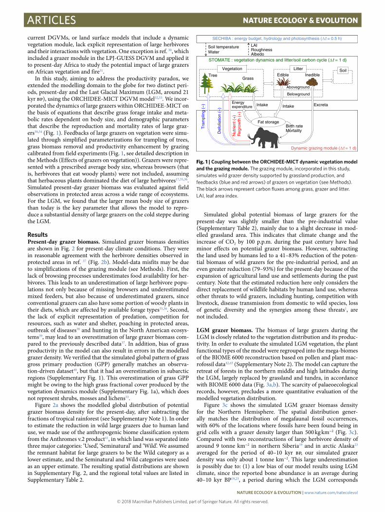
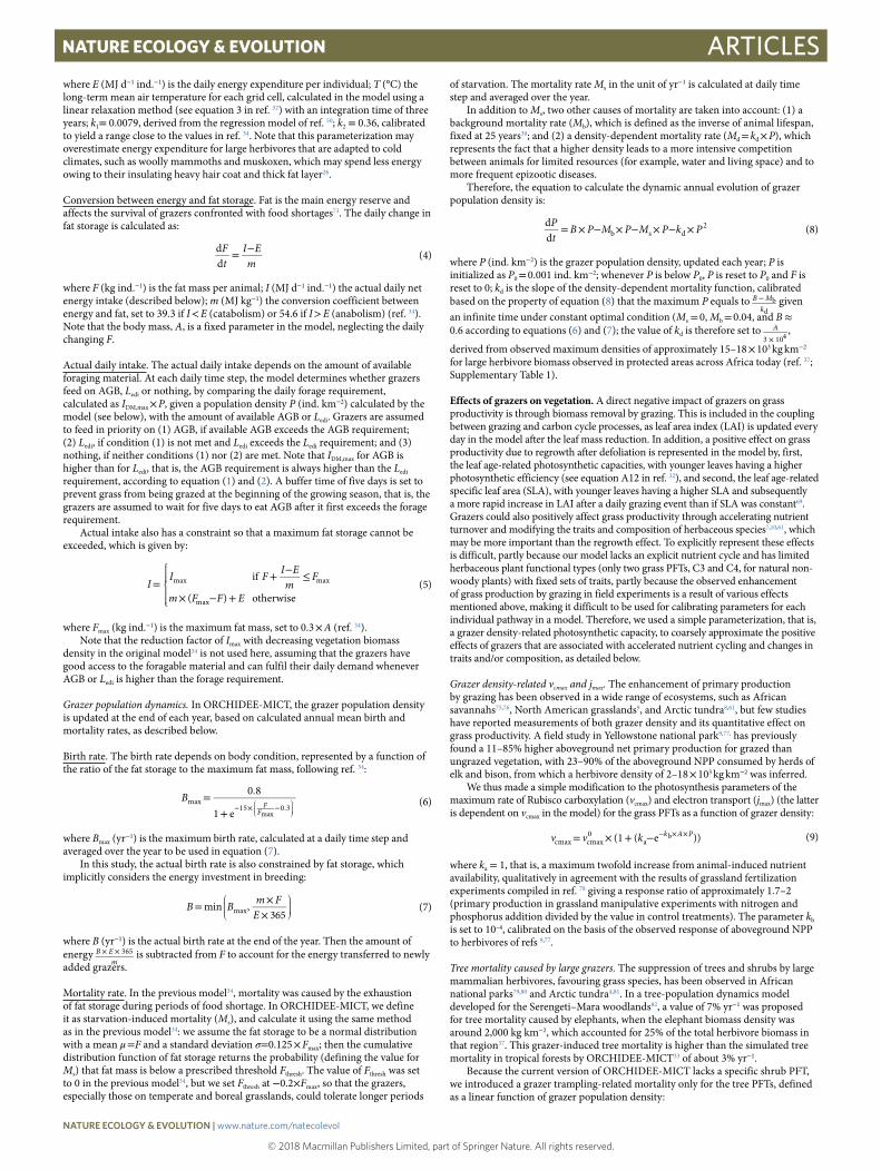
In this study, aiming to address the productivity paradox, we extended the modelling domain to the globe for two distinct peri-ods, present-day and the Last Glacial Maximum (LGM, around 21 kyr bp), using the ORCHIDEE-MICT DGVM model32,33. We incor-porated the dynamics of large grazers within ORCHIDEE-MICT on the basis of equations that describe grass forage intake and meta-bolic rates dependent on body size, and demographic parameters that describe the reproduction and mortality rates of large graz-ers30,34 (Fig. 1). Feedbacks of large grazers on vegetation were simu-lated through simplified parameterizations for trampling of trees, grass biomass removal and productivity enhancement by grazing calibrated from field experiments (Fig. 1, see detailed description in the Methods (Effects of grazers on vegetation)). Grazers were repre-sented with a prescribed average body size, whereas browsers (that is, herbivores that eat woody plants) were not included, assuming that herbaceous plants dominated the diet of large herbivores17,35,36. Simulated present-day grazer biomass was evaluated against field observations in protected areas across a wide range of ecosystems. For the LGM, we found that the larger mean body size of grazers than today is the key parameter that allows the model to repro-duce a substantial density of large grazers on the cold steppe during the LGM.

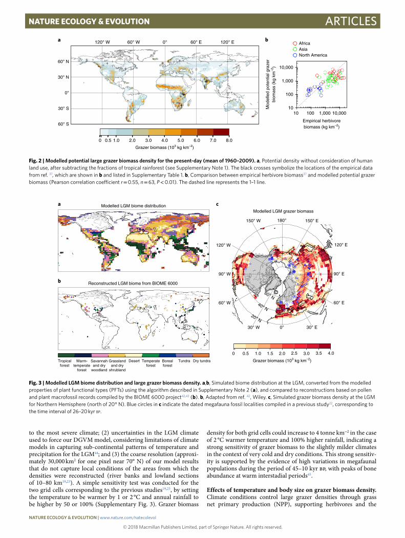
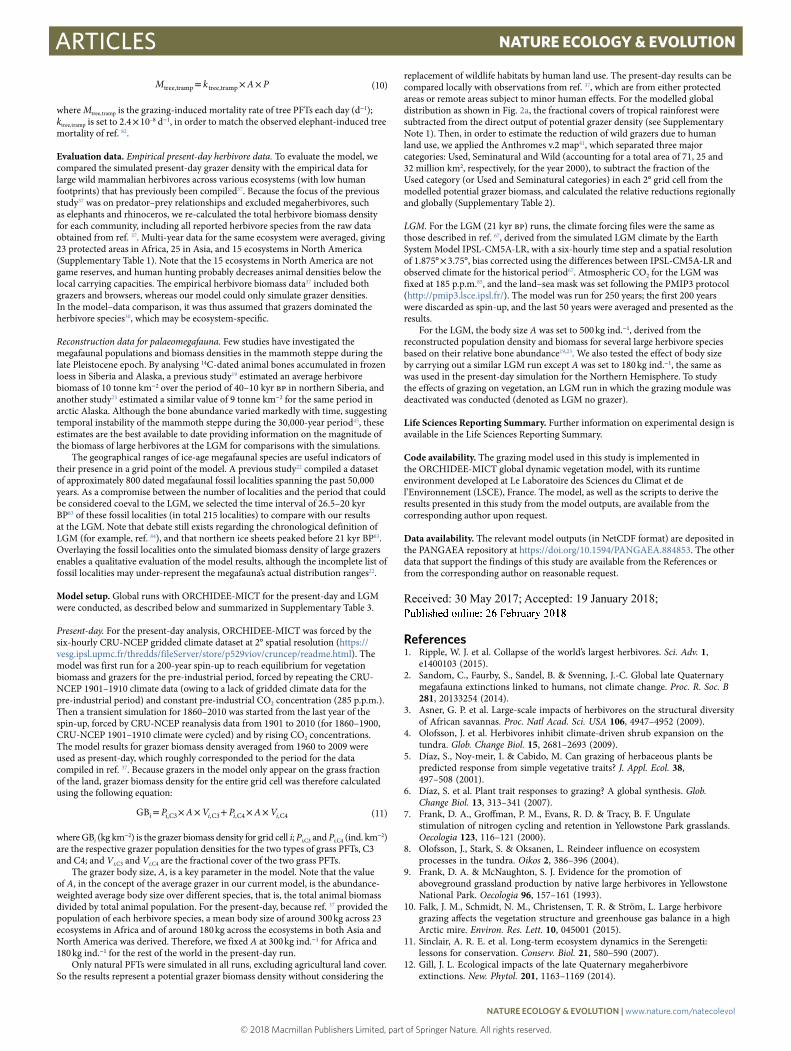
resultsPresent-day grazer biomass. Simulated grazer biomass densities are shown in Fig. 2 for present-day climate conditions. They were in reasonable agreement with the herbivore densities observed in protected areas in ref. 37 (Fig. 2b). Model-data misfits may be due to simplifications of the grazing module (see Methods). First, the lack of browsing processes underestimates food availability for her-bivores. This leads to an underestimation of large herbivore popu-lations not only because of missing browsers and underestimated mixed feeders, but also because of underestimated grazers, since conventional grazers can also have some portion of woody plants in their diets, which are affected by available forage types35,36. Second, the lack of explicit representation of predation, competition for resources, such as water and shelter, poaching in protected areas, outbreak of diseases38 and hunting in the North American ecosys-tems39, may lead to an overestimation of large grazer biomass com-pared to the previously described data37. In addition, bias of grass productivity in the model can also result in errors in the modelled grazer density. We verified that the simulated global pattern of grass gross primary production (GPP) generally matches an observa-tion-driven dataset40, but that it had an overestimation in subarctic regions (Supplementary Fig. 1). This overestimation of grass GPP might be owing to the high grass fractional cover produced by the vegetation dynamics module (Supplementary Fig. 1a), which does not represent shrubs, mosses and lichens33.

Figure 2a shows the modelled global distribution of potential grazer biomass density for the present-day, after subtracting the fractions of tropical rainforest (see Supplementary Note 1). In order to estimate the reduction in wild large grazers due to human land use, we made use of the anthropogenic biome classification system from the Anthromes v.2 product41, in which land was separated into three major categories: ‘Used’, ‘Seminatural’ and ‘Wild’. We assumed the remnant habitat for large grazers to be the Wild category as a lower estimate, and the Seminatural and Wild categories were used as an upper estimate. The resulting spatial distributions are shown in Supplementary Fig. 2, and the regional total values are listed in Supplementary Table 2.

Simulated global potential biomass of large grazers for the present-day was slightly smaller than the pre-industrial value (Supplementary Table 2), mainly due to a slight decrease in mod-elled grassland area. This indicates that climate change and the increase of CO2 by 100 p.p.m. during the past century have had minor effects on potential grazer biomass. However, subtracting the land used by humans led to a 41–83% reduction of the poten-tial biomass of wild grazers for the pre-industrial period, and an even greater reduction (79–93%) for the present-day because of the expansion of agricultural land use and settlements during the past century. Note that the estimated reduction here only considers the direct replacement of wildlife habitats by human land use, whereas other threats to wild grazers, including hunting, competition with livestock, disease transmission from domestic to wild species, loss of genetic diversity and the synergies among these threats1, are not included.

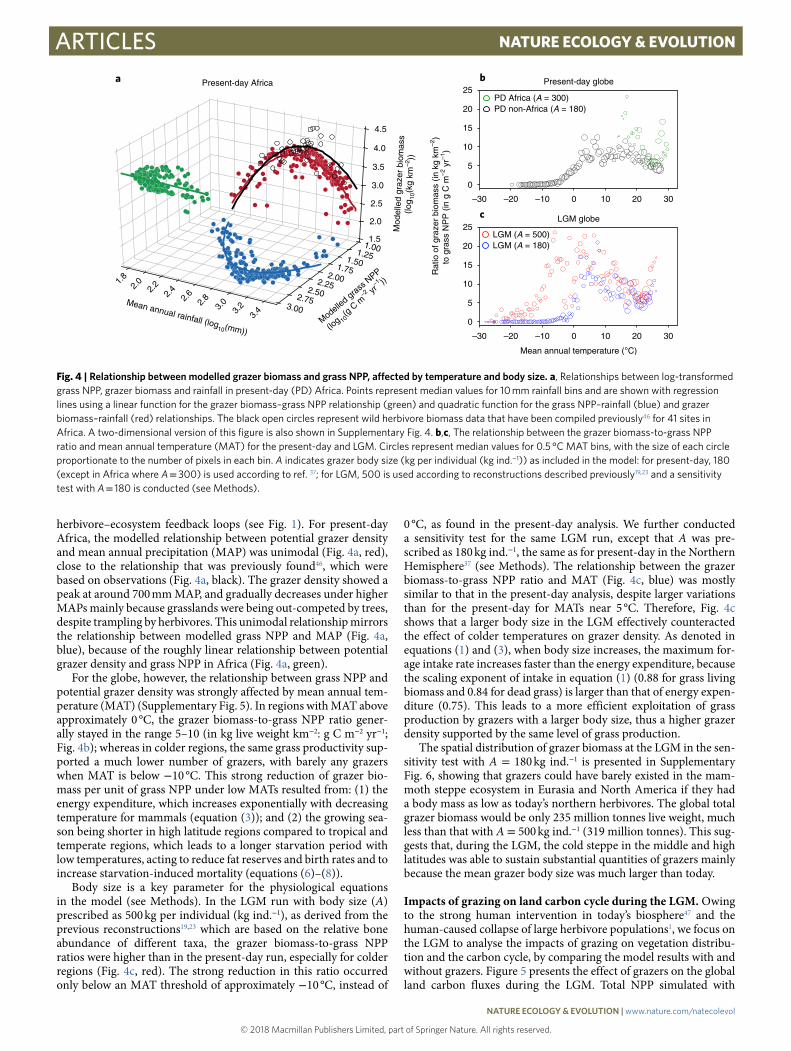
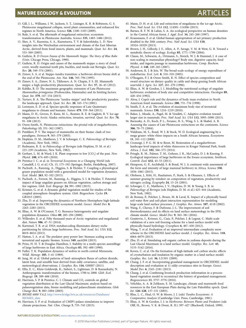
LGM grazer biomass. The biomass of large grazers during the LGM is closely related to the vegetation distribution and its produc-tivity. In order to evaluate the simulated LGM vegetation, the plant functional types of the model were regrouped into the mega-biomes of the BIOME 6000 reconstruction based on pollen and plant mac-rofossil data42,43 (Supplementary Note 2). The model can capture the retreat of forests in the northern middle and high latitudes during the LGM, largely replaced by grassland and tundra, in accordance with BIOME 6000 data (Fig. 3a,b). The scarcity of palaeoecological records, however, precludes a more quantitative evaluation of the modelled vegetation distribution.

Figure 3c shows the simulated LGM grazer biomass density for the Northern Hemisphere. The spatial distribution gener-ally matches the distribution of megafaunal fossil occurrences, with 60% of the locations where fossils have been found being in grid cells with a grazer density larger than 500 kg km−2 (Fig. 3c). Compared with two reconstructions of large herbivore density of around 9 tonne km−2 in northern Siberia19 and in arctic Alaska23 averaged for the period of 40–10 kyr bp, our simulated grazer density was only about 1 tonne km−2. This large underestimation is possibly due to: (1) a low bias of our model results using LGM climate, since the reported bone abundance is an average during 40–10 kyr BP19,23, a period during which the LGM corresponds

LAIRoughnessAlbedo

SECHIBA : energy budget, hydrology and photosynthesis (∆t = 0.5 h)

Soil temperatureWater

Vegetation

STOMATE : vegetation dynamics and litter/soil carbon cycle (∆t = 1 d)

Litter

Aboveground

Belowground

Soil

Dynamic grazing module (∆t = 1 d)

Intake Excreta

Fat storageBirth rateMortality

Nut

rient

(+

)R

egro

wth

(+

)

Tra

mpl

ing

(–)

Def

olia

tion

(–)

Edible Inedible

Intake

Tree

Energyexpenditure

Grass

Fig. 1 | Coupling between the orCHiDee-MiCT dynamic vegetation model and the grazing module. The grazing module, incorporated in this study, simulates wild grazer density supported by grassland production, and feedbacks (blue and red arrows) of grazers on vegetation (see Methods). The black arrows represent carbon fluxes among grass, grazer and litter. LAI, leaf area index.




ArticlesNaTure eCOLOGy & eVOLuTiON

to the most severe climate; (2) uncertainties in the LGM climate used to force our DGVM model, considering limitations of climate models in capturing sub-continental patterns of temperature and precipitation for the LGM44; and (3) the coarse resolution (approxi-mately 30,000 km2 for one pixel near 70° N) of our model results that do not capture local conditions of the areas from which the densities were reconstructed (river banks and lowland sections of 10–80 km19,23). A simple sensitivity test was conducted for the two grid cells corresponding to the previous studies19,23, by setting the temperature to be warmer by 1 or 2 °C and annual rainfall to be higher by 50 or 100% (Supplementary Fig. 3). Grazer biomass

density for both grid cells could increase to 4 tonne km−2 in the case of 2 °C warmer temperature and 100% higher rainfall, indicating a strong sensitivity of grazer biomass to the slightly milder climates in the context of very cold and dry conditions. This strong sensitiv-ity is supported by the evidence of high variations in megafaunal populations during the period of 45–10 kyr bp, with peaks of bone abundance at warm interstadial periods45.

Effects of temperature and body size on grazer biomass density. Climate conditions control large grazer densities through grass net primary production (NPP), supporting herbivores and the

Empirical herbivorebiomass (kg km–2)

Mod

elle

d po

tent

ial g

raze

rbi

omas

s (k

g km

–2)

10

100

1,000

10,00060° N

120° Wa b

0 0.5 1.0 2.0 3.0 4.0 5.0 6.0 7.0 8.0

60° W 0° 60° E 120° E

30° N

0°

30° S

60° S

10 100 1,000 10,000

AfricaAsiaNorth America

Grazer biomass (103 kg km–2)

Fig. 2 | Modelled potential large grazer biomass density for the present-day (mean of 1960–2009). a, Potential density without consideration of human land use, after subtracting the fractions of tropical rainforest (see Supplementary Note 1). The black crosses symbolize the locations of the empirical data from ref. 37, which are shown in b and listed in Supplementary Table 1. b, Comparison between empirical herbivore biomass37 and modelled potential grazer biomass (Pearson correlation coefficient r = 0.55, n = 63, P < 0.01). The dashed line represents the 1–1 line.

Tropicalforest

Warm-temperate

forest

Savannahand dry

woodland

Grasslandand dry

shrubland

Desert Temperateforest

Borealforest

Tundra Dry tundra Grazer biomass (103 kg km–2)

Modelled LGM biome distributiona c

b Reconstructed LGM biome from BIOME 6000

Modelled LGM grazer biomass

0 0.5 1.0 1.5 2.0 2.5 3.0 3.5 4.0

60° E

90° E

120° E

150° E180°150° W

120° W

90° W

60° W

60° N

40° N

20° N

30° W 30° E0°

Fig. 3 | Modelled LGM biome distribution and large grazer biomass density. a,b, Simulated biome distribution at the LGM, converted from the modelled properties of plant functional types (PFTs) using the algorithm described in Supplementary Note 2 (a), and compared to reconstructions based on pollen and plant macrofossil records compiled by the BIOME 6000 project42,43 (b). b, Adapted from ref. 42, Wiley. c, Simulated grazer biomass density at the LGM for Northern Hemisphere (north of 20° N). Blue circles in c indicate the dated megafauna fossil localities compiled in a previous study22, corresponding to the time interval of 26–20 kyr bp.





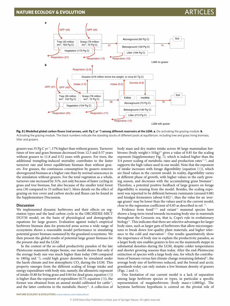
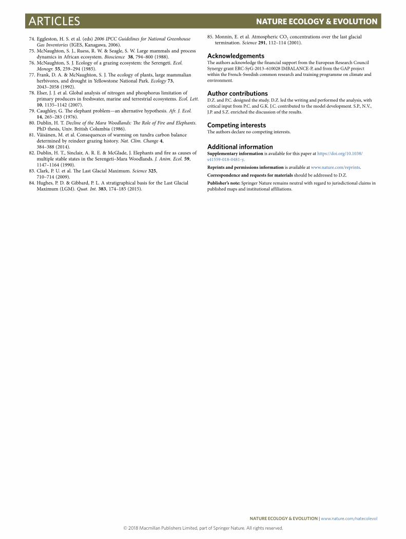
herbivore–ecosystem feedback loops (see Fig. 1). For present-day Africa, the modelled relationship between potential grazer density and mean annual precipitation (MAP) was unimodal (Fig. 4a, red), close to the relationship that was previously found46, which were based on observations (Fig. 4a, black). The grazer density showed a peak at around 700 mm MAP, and gradually decreases under higher MAPs mainly because grasslands were being out-competed by trees, despite trampling by herbivores. This unimodal relationship mirrors the relationship between modelled grass NPP and MAP (Fig. 4a, blue), because of the roughly linear relationship between potential grazer density and grass NPP in Africa (Fig. 4a, green).

For the globe, however, the relationship between grass NPP and potential grazer density was strongly affected by mean annual tem-perature (MAT) (Supplementary Fig. 5). In regions with MAT above approximately 0 °C, the grazer biomass-to-grass NPP ratio gener-ally stayed in the range 5–10 (in kg live weight km−2: g C m−2 yr−1; Fig. 4b); whereas in colder regions, the same grass productivity sup-ported a much lower number of grazers, with barely any grazers when MAT is below − 10 °C. This strong reduction of grazer bio-mass per unit of grass NPP under low MATs resulted from: (1) the energy expenditure, which increases exponentially with decreasing temperature for mammals (equation (3)); and (2) the growing sea-son being shorter in high latitude regions compared to tropical and temperate regions, which leads to a longer starvation period with low temperatures, acting to reduce fat reserves and birth rates and to increase starvation-induced mortality (equations (6)–(8)).

Body size is a key parameter for the physiological equations in the model (see Methods). In the LGM run with body size (A) prescribed as 500 kg per individual (kg ind.−1), as derived from the previous reconstructions19,23 which are based on the relative bone abundance of different taxa, the grazer biomass-to-grass NPP ratios were higher than in the present-day run, especially for colder regions (Fig. 4c, red). The strong reduction in this ratio occurred only below an MAT threshold of approximately − 10 °C, instead of

0 °C, as found in the present-day analysis. We further conducted a sensitivity test for the same LGM run, except that A was pre-scribed as 180 kg ind.−1, the same as for present-day in the Northern Hemisphere37 (see Methods). The relationship between the grazer biomass-to-grass NPP ratio and MAT (Fig. 4c, blue) was mostly similar to that in the present-day analysis, despite larger variations than for the present-day for MATs near 5 °C. Therefore, Fig. 4c shows that a larger body size in the LGM effectively counteracted the effect of colder temperatures on grazer density. As denoted in equations (1) and (3), when body size increases, the maximum for-age intake rate increases faster than the energy expenditure, because the scaling exponent of intake in equation (1) (0.88 for grass living biomass and 0.84 for dead grass) is larger than that of energy expen-diture (0.75). This leads to a more efficient exploitation of grass production by grazers with a larger body size, thus a higher grazer density supported by the same level of grass production.

The spatial distribution of grazer biomass at the LGM in the sen-sitivity test with A = 180 kg ind.−1 is presented in Supplementary Fig. 6, showing that grazers could have barely existed in the mam-moth steppe ecosystem in Eurasia and North America if they had a body mass as low as today’s northern herbivores. The global total grazer biomass would be only 235 million tonnes live weight, much less than that with A = 500 kg ind.−1 (319 million tonnes). This sug-gests that, during the LGM, the cold steppe in the middle and high latitudes was able to sustain substantial quantities of grazers mainly because the mean grazer body size was much larger than today.

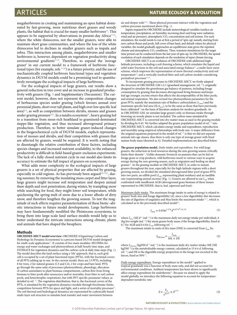
Impacts of grazing on land carbon cycle during the LGM. Owing to the strong human intervention in today’s biosphere47 and the human-caused collapse of large herbivore populations1, we focus on the LGM to analyse the impacts of grazing on vegetation distribu-tion and the carbon cycle, by comparing the model results with and without grazers. Figure 5 presents the effect of grazers on the global land carbon fluxes during the LGM. Total NPP simulated with

Mean annual rainfall (log10(mm))

Mod

elle

d gr

azer

bio

mas

s(lo

g 10(k

g km

–2))

Modelled gra

ss N

PP

(log 10

(g C

m–2 yr

–1 ))

Mean annual temperature (°C)

Rat

io o

f gra

zer

biom

ass

(in k

g km

–2)

to g

rass

NP

P (

in g

C m

–2 y

r–1)

PD Africa (A = 300)PD non-Africa (A = 180)

LGM (A = 500)LGM (A = 180)

Present-day Africa Present-day globe

LGM globe

a b

c

1.8

2.0

2.2

2.4

2.6

2.8

3.0

3.2

3.4

1.001.251.501.752.002.252.502.75

3.00

4.5

–30 –20 –10 0 10 20 30

–30 –20 –10 0 10 20 30

25

20

15

10

5

0

25

20

15

10

5

0

4.0

3.5

3.0

2.5

2.0

1.5

Fig. 4 | relationship between modelled grazer biomass and grass NPP, affected by temperature and body size. a, Relationships between log-transformed grass NPP, grazer biomass and rainfall in present-day (PD) Africa. Points represent median values for 10 mm rainfall bins and are shown with regression lines using a linear function for the grazer biomass–grass NPP relationship (green) and quadratic function for the grass NPP–rainfall (blue) and grazer biomass–rainfall (red) relationships. The black open circles represent wild herbivore biomass data that have been compiled previously46 for 41 sites in Africa. A two-dimensional version of this figure is also shown in Supplementary Fig. 4. b,c, The relationship between the grazer biomass-to-grass NPP ratio and mean annual temperature (MAT) for the present-day and LGM. Circles represent median values for 0.5 °C MAT bins, with the size of each circle proportionate to the number of pixels in each bin. A indicates grazer body size (kg per individual (kg ind.−1)) as included in the model: for present-day, 180 (except in Africa where A = 300) is used according to ref. 37; for LGM, 500 is used according to reconstructions described previously19,23 and a sensitivity test with A = 180 is conducted (see Methods).





grazers was 35 Pg C yr−1, 17% higher than without grazers. Turnover times of tree and grass biomass decreased from 12.5 and 0.57 years without grazers to 11.8 and 0.52 years with grazers. For trees, the additional trampling-induced mortality contributes to the faster turnover rate and lower equilibrium biomass than without graz-ers. For grasses, the continuous consumption by grazers removes aboveground biomass at a higher rate than by normal senescence in the simulation without grazers. For the total vegetation as a whole, turnover rate increased by 31%, not only because of faster cycling in grass and tree biomass, but also because of the smaller total forest area (30 compared to 33 million km2). More details on the effect of grazing on tree cover and carbon stocks and fluxes can be found in the Supplementary Discussion.

DiscussionWe implemented dynamic herbivores and their effects on veg-etation types and the land carbon cycle in the ORCHIDEE-MICT DGVM model, on the basis of physiological and demographic equations for large grazers. Evaluation against today’s empirical herbivore biomass data for protected areas across a wide range of ecosystems shows a reasonable model performance in simulating potential grazer biomass sustained by the grassland ecosystems. We then present the global results of potential large grazer biomass for the present-day and the LGM.

In the context of the so-called productivity paradox of the late Pleistocene mammoth steppe biome, our model shows that only if the average body size was much higher than today (500 compared to 180 kg ind.−1), could high grazer densities be simulated under the harsh climate and low atmospheric CO2 during the LGM. This property emerges from the different scaling of forage intake and energy expenditure with body size, namely, the allometric exponent of intake (0.88 for living grass and 0.84 for dead grass; equation (1)) is higher than the exponent of expenditure (0.75; equation (3)), the former was obtained from an animal model calibrated for cattle34, and the latter conforms to the metabolic theory48. A collection of

body mass and dry matter intake across 46 large mammalian her-bivores (body weight > 10 kg)49 gives a value of 0.85 for the scaling exponent (Supplementary Fig. 7), which is indeed higher than the 3/4 power scaling of metabolic rates and production rates37,50, and supports the high values used in our model. Note that the exponent of intake increases with forage digestibility (equation (1)), which are fixed values in the current model. In reality, digestibility varies at different phase of growth, with higher values in the early grow-ing season, and decreases with the accumulating grass biomass51. Therefore, a potential positive feedback of large grazers on forage digestibility is missing from the model. Besides, the scaling expo-nent was reported to be different between ruminants (around 0.88) and hindgut fermenters (about 0.82)52, thus the value for an 'aver-age grazer' may be lower than the values used in the current model, close to the regression coefficient of 0.85 as described in ref. 49.

Evidence from fossil53,54 and extant55 mammal species have shown a long-term trend towards increasing body size in mammals throughout the Cenozoic era, that is, Cope’s rule in evolutionary biology53. This indicates that there are selective advantages for larger body sizes, such as larger guts of herbivores that allow microorgan-isms to break down low-quality plant materials, and higher toler-ance to the cold and starvation55. Our results quantitatively show the importance of body size to explain the productivity paradox, as a larger body size enables grazers to live on the mammoth steppe in substantial densities during the LGM, despite colder temperatures and shorter growing seasons than today. After the end-Pleistocene extinction of species with a large body size, for which the contribu-tions of humans versus fast climate change remaining debated56, the average body size of herbivores reduced, and the boreal and arctic grasslands today can only sustain a low biomass density of grazers (Figs. 2 and 4).

One limitation of our current model is a lack of separation among large herbivore species or types, in particular a specific representation of megaherbivores (body mass > 1,000 kg). The keystone herbivore hypothesis is centred on the pivotal role of

a

b

Grass (79 millionkm2, 10 Pg C)

Tree (33 millionkm2, 163 Pg C)

Litter (194 Pg C)

Aboveground (65 Pg C)

Belowground (129 Pg C)

Soil

GPP (40)

Respiration (27)

31

Respiration (13)

14

GPP (30)

Vegetation (173 Pg C)

Respiration (13)LGM no grazer

Litter (213 Pg C)

InedibleEdible

Aboveground (73 Pg C)

Soil

Grazers (319 million tonne live weight, or circa 64 Tg C)

GPP (37)

Respiration (25)

Intake (1.5) Intake (0.2) Excreta (0.8)

36

Respiration (15)

Respiration (0.9)

16

Respiration (17)

GPP (40)

LGM with grazer

Belowground (140 Pg C)

Grass (78 millionkm2, 12 Pg C)

Tree (30 millionkm2, 142 Pg C)

Vegetation (154 Pg C)

Fig. 5 | Modelled global carbon fluxes (red arrows, unit: Pg C yr−1) among different reservoirs at the LGM. a, De-activating the grazing module. b, Activating the grazing module. The black numbers indicate the standing stocks of different pools at equilibrium, including tree and grass living biomass, litter and grazers.





megaherbivores in creating and maintaining an open habitat domi-nated by fast-growing, more nutritious short grasses and woody plants, the habitat that is crucial for many smaller herbivores24. This appears to be supported by observations in present-day Africa57,58, where the white rhinoceros, not the smaller grazers, were able to maintain short grass communities, and where the loss of the white rhinoceros led to declines in smaller grazers such as impala and zebra. This interaction among plants, megaherbivores and smaller herbivores is, however, dependent on vegetation productivity along environmental gradients57,59. Therefore, to expand the ‘average grazer’ in our current model to a framework of herbivore func-tional types (for example, refs 31,60) is a future priority; and the use of mechanistically coupled herbivore functional types and vegetation dynamics in DGVM models could be a promising tool to quantita-tively investigate the ecological impacts of large herbivores.

For the ecological impacts of large grazers, our results show a general reduction in tree cover and an increase in grassland produc-tivity with grazers (Fig. 5 and Supplementary Discussion). The cur-rent model, however, does not represent the composition changes of herbaceous species under grazing (which favours annual over perennial plants, short over tall plants, and high over low specific leaf area)5,6, as well as competition between shrubs, mosses and grasses under grazing pressure4,61. In a tundra ecosystem61, heavy grazing led to a transition from moss-rich heathland to graminoid-dominated steppe-like vegetation, and thus increased aboveground primary production. Therefore, to better simulate grazer-induced changes in the biogeochemical cycle of DGVM models, explicit representa-tion of mosses and shrubs, and their competition with grasses that are affected by grazers, would be required. It is worth noting that to disentangle the relative contribution of these factors, including species changes and increased nutrient availability, to the enhanced productivity is difficult in field-based grazer-exclusion experiments. The lack of a fully closed nutrient cycle in our model also limits its accuracy to estimate the full impact of grazers on ecosystems.

What adds more complexity to the ecological impacts of large grazers is a set of physical properties that are affected by grazing, especially in cold regions. As has previously been argued18,19,62, dur-ing summer, by removing the insulating moss carpet and litter layer, large grazers might increase soil temperature and deepen annual thaw depth and root penetration; during winter, by trampling snow while searching for food, they might lower soil temperature, while quickening the spring melt of snow due to a lower albedo of dirty snow, and therefore lengthen the growing season. To test the mag-nitude of such effects requires parameterization of these biotic–abi-otic interactions in future model developments. Large herbivores may have fundamentally modified the Pleistocene ecosystems; to bring them into large-scale land surface models would help us to better understand the intricate interactions among climate, plants and animals that have shaped the biosphere.

MethodsORCHIDEE-MICT model overview. ORCHIDEE (Organizing Carbon and Hydrology In Dynamic Ecosystems) is a process-based DGVM model designed for multi-scale applications32. It consists of two main modules: SECHIBA for energy and water exchanges and photosynthesis at half-hourly time steps, and STOMATE for vegetation dynamics and the carbon cycle at daily time steps (Fig. 1). The model describes the land surface using a ‘tile’ approach, that is, each grid cell is occupied by a set of plant functional types (PFTs), with the fractional covers of all PFTs adding up to one. In the current model, there are 13 PFTs, including 8 for trees, 2 for natural grasses (C3 and C4), 2 for crops and bare land. PFTs go through the same suite of processes (photosynthesis, phenology, allocation of carbon assimilates to plant biomass compartments, carbon flow from living biomass to litter pools after senescence and/or mortality, from litter to soil carbon pools, and heterotrophic respiration), but with PFT-specific parameter values, as detailed in ref. 32. The vegetation distribution, that is, the fractional covers of the PFTs, is simulated by the vegetation dynamics module through bioclimatic limits, competition between PFTs for space and light, and a series of mortality processes33. The soil thermal and hydrological dynamics are represented by a physically based multi-layer soil structure to simulate heat transfer and water movement between

air and deeper soils63,64. These physical processes interact with the vegetation and carbon processes mentioned above (Fig. 1).

Inputs required by ORCHIDEE include meteorological variables (surface air temperature, precipitation, air humidity, incoming short and long wave radiation, wind and air pressure), atmospheric CO2 concentration and soil texture. For each simulation, the model needs to run at first a period of ‘spin-up’, namely, starting from zero carbon fluxes and pools, full cover of bare land, and default values for physical variables, the model gradually approaches an equilibrium state given the inputted climate and atmospheric CO2 conditions. Then, transient simulations for the target time period can be conducted from the last year of spin-up. In ORCHIDEE, the spatial resolution of each simulation depends on the resolution of input climate forcing.

ORCHIDEE-MICT is an evolution of ORCHIDEE with additional high-latitude processes, including a soil-freezing scheme, which simulates the liquid and solid water fractions in the soil and associated energy balance65, a multi-layer snow scheme, which improves the representation of snow thermal conductivity and soil temperature66, and a vertically resolved litter and soil carbon module considering permafrost processes67,68.

To incorporate grazing processes in ORCHIDEE-MICT, we firstly adapted the structure of ORCHIDEE-GM v.2.1 (grassland management, ref. 69), originally designed to simulate the greenhouse gas balance of pastures, including forage consumption by grazing that decreases aboveground living biomass and keeps leaf age younger, excreta return that affects the decomposability of the litter pools, and animal respiration. We also revised two photosynthesis parameters for the grass PFTs, namely the maximum rate of Rubisco carboxylation (vcmax) and the maximum specific leaf area (SLAmax), to be the same as those that have previously been calibrated70 on the basis of literature analysis for modern grasslands. As in ORCHIDEE-GM, we simulate large grazers only, so biomass intake through browsing on woody plants is not included. The carbon mass simulated by ORCHIDEE-MICT is converted into dry matter mass as used in the grazing module by dividing by 0.45. We further adapted the grazer population model of ref. 34 into ORCHIDEE-MICT, which calculates energy intake and expenditure, reproduction and mortality using empirical relationships with body size. A major difference from the original equations proposed in the model of ref. 34 is that we did not separate animals into age classes, thus there is only one type of average grazer with fixed mature body mass (denoted as A). Detailed implementations are described below.

The grazer population model. Daily intake and expenditure. For wild large grazers, the reduction in food resources during the non-growing season critically limits their density71. Unlike domestic livestock on pastures that can be fed on forage grass or crop products, wild herbivores resort to various ways to acquire energy during the non-growing season, such as migration and feeding on dead grasses72. In the grazing module in ORCHIDEE-MICT, in order to sustain grazers throughout the year, especially for the high-latitude regions with a short growing season, we divided the simulated aboveground litter pool of grass PFTs into two parts, an edible pool (Ledi, representing plant residues) and an inedible one (representing animal excreta) (Fig. 1). Grazers are allowed to eat Ledi when confronted with insufficient AGB (aboveground grass biomass of three tissues represented in ORCHIDEE, that is, leaf, sapwood and fruit).

Maximum daily intake. The maximum forage intake in units of energy is related to grazers’ body size and forage digestibility (d), since a low digestibility diet decreases the rate of digestion of ungulates and thus limits the maximum intake52,73, which is calculated as in the previously described model34:

= . . . + .I A0 034e (1)dmax

3 57 (0 077e 0 73)d

where Imax (MJ d−1 ind.−1) is the maximum daily net energy intake per individual; A (kg live weight ind.−1) the mean grazer body mass; d the forage digestibility, fixed at 0.7 for AGB and 0.4 for Ledi, following ref. 34.

The maximum intake in units of dry mass (DM) is converted from Imax by:

= ×

II

ME DE(2)DM,max

max

where IDM,max (kgDM d−1 ind.−1) is the maximum daily dry matter intake; ME (MJ kgDM−1) is the metabolizable energy content, calculated as 15.6 × d, following ref. 30; and DE is the digestible energy proportion in the forage not excreted in the faeces, fixed as 50%74.

Daily energy expenditure. Energy expenditure in the model34 applied to tropical grasslands was a function of body mass only, and did not account for environmental conditions. Ambient temperature has been shown to significantly affect energy expenditure for endotherms50. Because we aimed to apply the model globally, we introduce the following equation to account for temperature-dependent metabolic rate:

= ××.E

kA

e(3)k T

2 0 751





where E (MJ d−1 ind.−1) is the daily energy expenditure per individual; T (°C) the long-term mean air temperature for each grid cell, calculated in the model using a linear relaxation method (see equation 3 in ref. 32) with an integration time of three years; k1= 0.0079, derived from the regression model of ref. 50; k2 = 0.36, calibrated to yield a range close to the values in ref. 34. Note that this parameterization may overestimate energy expenditure for large herbivores that are adapted to cold climates, such as woolly mammoths and muskoxen, which may spend less energy owing to their insulating heavy hair coat and thick fat layer26.

Conversion between energy and fat storage. Fat is the main energy reserve and affects the survival of grazers confronted with food shortages73. The daily change in fat storage is calculated as:

= −Ft

I Em

dd

(4)

where F (kg ind.−1) is the fat mass per animal; I (MJ d−1 ind.−1) the actual daily net energy intake (described below); m (MJ kg−1) the conversion coefficient between energy and fat, set to 39.3 if I < E (catabolism) or 54.6 if I > E (anabolism) (ref. 34). Note that the body mass, A, is a fixed parameter in the model, neglecting the daily changing F.

Actual daily intake. The actual daily intake depends on the amount of available foraging material. At each daily time step, the model determines whether grazers feed on AGB, Ledi or nothing, by comparing the daily forage requirement, calculated as IDM,max × P, given a population density P (ind. km−2) calculated by the model (see below), with the amount of available AGB or Ledi. Grazers are assumed to feed in priority on (1) AGB, if available AGB exceeds the AGB requirement; (2) Ledi, if condition (1) is not met and Ledi exceeds the Ledi requirement; and (3) nothing, if neither conditions (1) nor (2) are met. Note that IDM,max for AGB is higher than for Ledi, that is, the AGB requirement is always higher than the Ledi requirement, according to equation (1) and (2). A buffer time of five days is set to prevent grass from being grazed at the beginning of the growing season, that is, the grazers are assumed to wait for five days to eat AGB after it first exceeds the forage requirement.

Actual intake also has a constraint so that a maximum fat storage cannot be exceeded, which is given by:

=+ − ≤

× − +

II F I E

mF

m F F E

if

( ) otherwise(5)max max

max

where Fmax (kg ind.−1) is the maximum fat mass, set to 0.3 × A (ref. 34).Note that the reduction factor of Imax with decreasing vegetation biomass

density in the original model34 is not used here, assuming that the grazers have good access to the foragable material and can fulfil their daily demand whenever AGB or Ledi is higher than the forage requirement.

Grazer population dynamics. In ORCHIDEE-MICT, the grazer population density is updated at the end of each year, based on calculated annual mean birth and mortality rates, as described below.

Birth rate. The birth rate depends on body condition, represented by a function of the ratio of the fat storage to the maximum fat mass, following ref. 34:

= .

+ − × − .

B 0 8

1 e(6)max

15 0 3FFmax

where Bmax (yr−1) is the maximum birth rate, calculated at a daily time step and averaged over the year to be used in equation (7).

In this study, the actual birth rate is also constrained by fat storage, which implicitly considers the energy investment in breeding:

= ××

B B m F

Emin ,

365(7)max

where B (yr−1) is the actual birth rate at the end of the year. Then the amount of energy × ×B E

m365 is subtracted from F to account for the energy transferred to newly

added grazers.

Mortality rate. In the previous model34, mortality was caused by the exhaustion of fat storage during periods of food shortage. In ORCHIDEE-MICT, we define it as starvation-induced mortality (Ms), and calculate it using the same method as in the previous model34: we assume the fat storage to be a normal distribution with a mean μ = F and a standard deviation σ= 0.125 × Fmax; then the cumulative distribution function of fat storage returns the probability (defining the value for Ms) that fat mass is below a prescribed threshold Fthresh. The value of Fthresh was set to 0 in the previous model34, but we set Fthresh at − 0.2× Fmax, so that the grazers, especially those on temperate and boreal grasslands, could tolerate longer periods

of starvation. The mortality rate Ms in the unit of yr−1 is calculated at daily time step and averaged over the year.

In addition to Ms, two other causes of mortality are taken into account: (1) a background mortality rate (Mb), which is defined as the inverse of animal lifespan, fixed at 25 years30; and (2) a density-dependent mortality rate (Md = kd × P), which represents the fact that a higher density leads to a more intensive competition between animals for limited resources (for example, water and living space) and to more frequent epizootic diseases.

Therefore, the equation to calculate the dynamic annual evolution of grazer population density is:

= × − × − × − ×Pt

B P M P M P k Pdd

(8)b s d2

where P (ind. km−2) is the grazer population density, updated each year; P is initialized as P0 = 0.001 ind. km−2; whenever P is below P0, P is reset to P0 and F is reset to 0; kd is the slope of the density-dependent mortality function, calibrated based on the property of equation (8) that the maximum P equals to −B M

kb

d given

an infinite time under constant optimal condition (Ms = 0, Mb = 0.04, and B ≈ 0.6 according to equations (6) and (7); the value of kd is therefore set to

×A

3 104 ,

derived from observed maximum densities of approximately 15–18 × 103 kg km−2 for large herbivore biomass observed in protected areas across Africa today (ref. 37; Supplementary Table 1).

Effects of grazers on vegetation. A direct negative impact of grazers on grass productivity is through biomass removal by grazing. This is included in the coupling between grazing and carbon cycle processes, as leaf area index (LAI) is updated every day in the model after the leaf mass reduction. In addition, a positive effect on grass productivity due to regrowth after defoliation is represented in the model by, first, the leaf age-related photosynthetic capacities, with younger leaves having a higher photosynthetic efficiency (see equation A12 in ref. 32), and second, the leaf age-related specific leaf area (SLA), with younger leaves having a higher SLA and subsequently a more rapid increase in LAI after a daily grazing event than if SLA was constant69. Grazers could also positively affect grass productivity through accelerating nutrient turnover and modifying the traits and composition of herbaceous species7,10,61, which may be more important than the regrowth effect. To explicitly represent these effects is difficult, partly because our model lacks an explicit nutrient cycle and has limited herbaceous plant functional types (only two grass PFTs, C3 and C4, for natural non-woody plants) with fixed sets of traits, partly because the observed enhancement of grass production by grazing in field experiments is a result of various effects mentioned above, making it difficult to be used for calibrating parameters for each individual pathway in a model. Therefore, we used a simple parameterization, that is, a grazer density-related photosynthetic capacity, to coarsely approximate the positive effects of grazers that are associated with accelerated nutrient cycling and changes in traits and/or composition, as detailed below.

Grazer density-related vcmax and jmax. The enhancement of primary production by grazing has been observed in a wide range of ecosystems, such as African savannahs75,76, North American grasslands9, and Arctic tundra8,61, but few studies have reported measurements of both grazer density and its quantitative effect on grass productivity. A field study in Yellowstone national park9,77, has previously found a 11–85% higher aboveground net primary production for grazed than ungrazed vegetation, with 23–90% of the aboveground NPP consumed by herds of elk and bison, from which a herbivore density of 2–18 × 103 kg km−2 was inferred.

We thus made a simple modification to the photosynthesis parameters of the maximum rate of Rubisco carboxylation (vcmax) and electron transport (jmax) (the latter is dependent on vcmax in the model) for the grass PFTs as a function of grazer density:

= × + − − × ×v v k(1 ( e )) (9)k A Pcmax cmax

0a

b

where ka = 1, that is, a maximum twofold increase from animal-induced nutrient availability, qualitatively in agreement with the results of grassland fertilization experiments compiled in ref. 78 giving a response ratio of approximately 1.7–2 (primary production in grassland manipulative experiments with nitrogen and phosphorus addition divided by the value in control treatments). The parameter kb is set to 10–4, calibrated on the basis of the observed response of aboveground NPP to herbivores of refs 9,77.

Tree mortality caused by large grazers. The suppression of trees and shrubs by large mammalian herbivores, favouring grass species, has been observed in African national parks79,80 and Arctic tundra4,81. In a tree-population dynamics model developed for the Serengeti–Mara woodlands82, a value of 7% yr−1 was proposed for tree mortality caused by elephants, when the elephant biomass density was around 2,000 kg km−2, which accounted for 25% of the total herbivore biomass in that region37. This grazer-induced tree mortality is higher than the simulated tree mortality in tropical forests by ORCHIDEE-MICT33 of about 3% yr−1.

Because the current version of ORCHIDEE-MICT lacks a specific shrub PFT, we introduced a grazer trampling-related mortality only for the tree PFTs, defined as a linear function of grazer population density:





= × ×M k A P (10)tree,tramp tree,tramp

where Mtree,tramp is the grazing-induced mortality rate of tree PFTs each day (d−1); ktree,tramp is set to 2.4 × 10–8 d−1, in order to match the observed elephant-induced tree mortality of ref. 82.

Evaluation data. Empirical present-day herbivore data. To evaluate the model, we compared the simulated present-day grazer density with the empirical data for large wild mammalian herbivores across various ecosystems (with low human footprints) that has previously been compiled37. Because the focus of the previous study37 was on predator–prey relationships and excluded megaherbivores, such as elephants and rhinoceros, we re-calculated the total herbivore biomass density for each community, including all reported herbivore species from the raw data obtained from ref. 37. Multi-year data for the same ecosystem were averaged, giving 23 protected areas in Africa, 25 in Asia, and 15 ecosystems in North America (Supplementary Table 1). Note that the 15 ecosystems in North America are not game reserves, and human hunting probably decreases animal densities below the local carrying capacities. The empirical herbivore biomass data37 included both grazers and browsers, whereas our model could only simulate grazer densities. In the model–data comparison, it was thus assumed that grazers dominated the herbivore species30, which may be ecosystem-specific.

Reconstruction data for palaeomegafauna. Few studies have investigated the megafaunal populations and biomass densities in the mammoth steppe during the late Pleistocene epoch. By analysing 14C-dated animal bones accumulated in frozen loess in Siberia and Alaska, a previous study19 estimated an average herbivore biomass of 10 tonne km−2 over the period of 40–10 kyr bp in northern Siberia, and another study23 estimated a similar value of 9 tonne km−2 for the same period in arctic Alaska. Although the bone abundance varied markedly with time, suggesting temporal instability of the mammoth steppe during the 30,000-year period45, these estimates are the best available to date providing information on the magnitude of the biomass of large herbivores at the LGM for comparisons with the simulations.

The geographical ranges of ice-age megafaunal species are useful indicators of their presence in a grid point of the model. A previous study22 compiled a dataset of approximately 800 dated megafaunal fossil localities spanning the past 50,000 years. As a compromise between the number of localities and the period that could be considered coeval to the LGM, we selected the time interval of 26.5–20 kyr BP83 of these fossil localities (in total 215 localities) to compare with our results at the LGM. Note that debate still exists regarding the chronological definition of LGM (for example, ref. 84), and that northern ice sheets peaked before 21 kyr BP83. Overlaying the fossil localities onto the simulated biomass density of large grazers enables a qualitative evaluation of the model results, although the incomplete list of fossil localities may under-represent the megafauna’s actual distribution ranges22.

Model setup. Global runs with ORCHIDEE-MICT for the present-day and LGM were conducted, as described below and summarized in Supplementary Table 3.

Present-day. For the present-day analysis, ORCHIDEE-MICT was forced by the six-hourly CRU-NCEP gridded climate dataset at 2° spatial resolution (https://vesg.ipsl.upmc.fr/thredds/fileServer/store/p529viov/cruncep/readme.html). The model was first run for a 200-year spin-up to reach equilibrium for vegetation biomass and grazers for the pre-industrial period, forced by repeating the CRU-NCEP 1901–1910 climate data (owing to a lack of gridded climate data for the pre-industrial period) and constant pre-industrial CO2 concentration (285 p.p.m.). Then a transient simulation for 1860–2010 was started from the last year of the spin-up, forced by CRU-NCEP reanalysis data from 1901 to 2010 (for 1860–1900, CRU-NCEP 1901–1910 climate were cycled) and by rising CO2 concentrations. The model results for grazer biomass density averaged from 1960 to 2009 were used as present-day, which roughly corresponded to the period for the data compiled in ref. 37. Because grazers in the model only appear on the grass fraction of the land, grazer biomass density for the entire grid cell was therefore calculated using the following equation:

= × × + × ×P A V P A VGB (11)i i i i i,C3 ,C3 ,C4 ,C4

where GBi (kg km−2) is the grazer biomass density for grid cell i; Pi,C3 and Pi,C4 (ind. km−2) are the respective grazer population densities for the two types of grass PFTs, C3 and C4; and Vi,C3 and Vi,C4 are the fractional cover of the two grass PFTs.

The grazer body size, A, is a key parameter in the model. Note that the value of A, in the concept of the average grazer in our current model, is the abundance-weighted average body size over different species, that is, the total animal biomass divided by total animal population. For the present-day, because ref. 37 provided the population of each herbivore species, a mean body size of around 300 kg across 23 ecosystems in Africa and of around 180 kg across the ecosystems in both Asia and North America was derived. Therefore, we fixed A at 300 kg ind.−1 for Africa and 180 kg ind.−1 for the rest of the world in the present-day run.

Only natural PFTs were simulated in all runs, excluding agricultural land cover. So the results represent a potential grazer biomass density without considering the

replacement of wildlife habitats by human land use. The present-day results can be compared locally with observations from ref. 37, which are from either protected areas or remote areas subject to minor human effects. For the modelled global distribution as shown in Fig. 2a, the fractional covers of tropical rainforest were subtracted from the direct output of potential grazer density (see Supplementary Note 1). Then, in order to estimate the reduction of wild grazers due to human land use, we applied the Anthromes v.2 map41, which separated three major categories: Used, Seminatural and Wild (accounting for a total area of 71, 25 and 32 million km2, respectively, for the year 2000), to subtract the fraction of the Used category (or Used and Seminatural categories) in each 2° grid cell from the modelled potential grazer biomass, and calculated the relative reductions regionally and globally (Supplementary Table 2).

LGM. For the LGM (21 kyr bp) runs, the climate forcing files were the same as those described in ref. 67, derived from the simulated LGM climate by the Earth System Model IPSL-CM5A-LR, with a six-hourly time step and a spatial resolution of 1.875° × 3.75°, bias corrected using the differences between IPSL-CM5A-LR and observed climate for the historical period67. Atmospheric CO2 for the LGM was fixed at 185 p.p.m.85, and the land–sea mask was set following the PMIP3 protocol (http://pmip3.lsce.ipsl.fr/). The model was run for 250 years; the first 200 years were discarded as spin-up, and the last 50 years were averaged and presented as the results.

For the LGM, the body size A was set to 500 kg ind.−1, derived from the reconstructed population density and biomass for several large herbivore species based on their relative bone abundance19,23. We also tested the effect of body size by carrying out a similar LGM run except A was set to 180 kg ind.−1, the same as was used in the present-day simulation for the Northern Hemisphere. To study the effects of grazing on vegetation, an LGM run in which the grazing module was deactivated was conducted (denoted as LGM no grazer).

Life Sciences Reporting Summary. Further information on experimental design is available in the Life Sciences Reporting Summary.

Code availability. The grazing model used in this study is implemented in the ORCHIDEE-MICT global dynamic vegetation model, with its runtime environment developed at Le Laboratoire des Sciences du Climat et de l’Environnement (LSCE), France. The model, as well as the scripts to derive the results presented in this study from the model outputs, are available from the corresponding author upon request.

Data availability. The relevant model outputs (in NetCDF format) are deposited in the PANGAEA repository at https://doi.org/10.1594/PANGAEA.884853. The other data that support the findings of this study are available from the References or from the corresponding author on reasonable request.

Received: 30 May 2017; Accepted: 19 January 2018; Published: xx xx xxxx

references 1. Ripple, W. J. et al. Collapse of the world’s largest herbivores. Sci. Adv. 1,

e1400103 (2015). 2. Sandom, C., Faurby, S., Sandel, B. & Svenning, J.-C. Global late Quaternary

megafauna extinctions linked to humans, not climate change. Proc. R. Soc. B 281, 20133254 (2014).

3. Asner, G. P. et al. Large-scale impacts of herbivores on the structural diversity of African savannas. Proc. Natl Acad. Sci. USA 106, 4947–4952 (2009).

4. Olofsson, J. et al. Herbivores inhibit climate-driven shrub expansion on the tundra. Glob. Change Biol. 15, 2681–2693 (2009).

5. Díaz, S., Noy-meir, I. & Cabido, M. Can grazing of herbaceous plants be predicted response from simple vegetative traits? J. Appl. Ecol. 38, 497–508 (2001).

6. Díaz, S. et al. Plant trait responses to grazing? A global synthesis. Glob. Change Biol. 13, 313–341 (2007).

7. Frank, D. A., Groffman, P. M., Evans, R. D. & Tracy, B. F. Ungulate stimulation of nitrogen cycling and retention in Yellowstone Park grasslands. Oecologia 123, 116–121 (2000).

8. Olofsson, J., Stark, S. & Oksanen, L. Reindeer influence on ecosystem processes in the tundra. Oikos 2, 386–396 (2004).

9. Frank, D. A. & McNaughton, S. J. Evidence for the promotion of aboveground grassland production by native large herbivores in Yellowstone National Park. Oecologia 96, 157–161 (1993).

10. Falk, J. M., Schmidt, N. M., Christensen, T. R. & Ström, L. Large herbivore grazing affects the vegetation structure and greenhouse gas balance in a high Arctic mire. Environ. Res. Lett. 10, 045001 (2015).

11. Sinclair, A. R. E. et al. Long-term ecosystem dynamics in the Serengeti: lessons for conservation. Conserv. Biol. 21, 580–590 (2007).

12. Gill, J. L. Ecological impacts of the late Quaternary megaherbivore extinctions. New. Phytol. 201, 1163–1169 (2014).


https://vesg.ipsl.upmc.fr/thredds/fileServer/store/p529viov/cruncep/readme.html

https://vesg.ipsl.upmc.fr/thredds/fileServer/store/p529viov/cruncep/readme.html

http://pmip3.lsce.ipsl.fr/

https://doi.org/10.1594/PANGAEA.884853




45. Mann, D. H. et al. Life and extinction of megafauna in the ice-age Arctic. Proc. Natl Acad. Sci. USA 112, 114301–114306 (2015).

46. Barnes, R. F. W. & Lahm, S. A. An ecological perspective on human densities in the Central African forest. J. Appl. Ecol. 34, 245–260 (1997).

47. Krausmann, F. et al. Global human appropriation of net primary production doubled in the 20th century. Proc. Natl Acad. Sci. USA 110, 10324–10329 (2013).

48. Brown, J. H., Gillooly, J. F., Allen, A. P., Savage, V. M. & West, G. B. Toward a metabolic theory of ecology. Ecology 85, 1771–1789 (2004).

49. Clauss, M., Schwarm, A., Ortmann, S., Streich, W. J. & Hummel, J. A case of non-scaling in mammalian physiology? Body size, digestive capacity, food intake, and ingesta passage in mammalian herbivores. Comp. Biochem. Physiol. A 148, 249–265 (2007).

50. Anderson, K. J. & Jetz, W. The broad-scale ecology of energy expenditure of endotherms. Ecol. Lett. 8, 310–318 (2005).

51. O’Reagain, P. J. & Owen-Smith, R. N. Effect of species composition and sward structure on dietary quality in cattle and sheep grazing South African sourveld. J. Agric. Sci. 127, 261–270 (1996).

52. Illius, A. W. & Gordon, I. J. Modelling the nutritional ecology of ungulate herbivores: evolution of body size and competitive interactions. Oecologia 89, 428–434 (1992).

53. Alroy, J. Cope’s rule and the dynamics of body mass evolution in North American fossil mammals. Science 280, 731–734 (1998).

54. Smith, F. A. et al. The evolution of maximum body size of terrestrial mammals. Science 330, 1216–1219 (2010).

55. Baker, J., Meade, A., Pagel, M. & Venditti, C. Adaptive evolution toward larger size in mammals. Proc. Natl Acad. Sci. USA 112, 5093–5098 (2015).

56. Barnosky, A. D., Koch, P. L., Feranec, R. S., Wing, S. L. & Shabel, A. B. Assessing the causes of Late Pleistocene extinctions on the continents. Science 306, 70–75 (2004).

57. Waldram, M. S., Bond, W. J. & Stock, W. D. Ecological engineering by a mega-grazer: white rhino impacts on a South African Savanna. Ecosystems 11, 101–112 (2008).

58. Cromsigt, J. P. G. M. & te Beest, M. Restoration of a megaherbivore: landscape-level impacts of white rhinoceros in Kruger National Park, South Africa. J. Ecol. 102, 566–575 (2014).

59. Pringle, R. M., Palmer, T. M., Goheen, J. R., McCauley, D. J. & Keesing, F. Ecological importance of large herbivores in the Ewaso ecosystem. Smithson. Contrib. Zool. 632, 43–53 (2011).

60. Hempson, G. P., Archibald, S. & Bond, W. J. A continent-wide assessment of the form and intensity of large mammal herbivory in Africa. Science 350, 1056–1061 (2015).

61. Olofsson, J., Kitti, H., Rautiainen, P., Stark, S. & Oksanen, L. Effects of summer grazing by reindeer on composition of vegetation, productivity and nitrogen cycling. Ecography 24, 13–24 (2001).

62. Schweger, C. E., Matthews, J. V., Hopkins, D. M. & Young, S. B. in Paleoecology of Beringia (eds Hopkins, D. M. et al.) 425–444 (Academic, New York, 1982).

63. de Rosnay, P., Polcher, J., Bruen, M. & Laval, K. Impact of a physically based soil water flow and soil-plant interaction representation for modeling large-scale land surface processes. J. Geophys. Res. Atmos. 107, 4118 (2002).

64. Wang, F., Cheruy, F. & Dufresne, J.-L. The improvement of soil thermodynamics and its effects on land surface meteorology in the IPSL climate model. Geosci. Model Dev. 9, 363–381 (2016).

65. Gouttevin, I., Krinner, G., Ciais, P., Polcher, J. & Legout, C. Multi-scale validation of a new soil freezing scheme for a land-surface model with physically-based hydrology. Cryosphere 6, 407–430 (2012).

66. Wang, T. et al. Evaluation of an improved intermediate complexity snow scheme in the ORCHIDEE land surface model. J. Geophys. Res. Atmos. 118, 6064–6079 (2013).

67. Zhu, D. et al. Simulating soil organic carbon in yedoma deposits during the Last Glacial Maximum in a land surface model. Geophys. Res. Lett. 43, 5133–5142 (2016).

68. Koven, C. et al. On the formation of high-latitude soil carbon stocks: effects of cryoturbation and insulation by organic matter in a land surface model. Geophys. Res. Lett. 36, L21501 (2009).

69. Chang, J. F. et al. Incorporating grassland management in ORCHIDEE: model description and evaluation at 11 eddy-covariance sites in Europe. Geosci. Model Dev. 6, 2165–2181 (2013).

70. Chang, J. et al. Combining livestock production information in a process-based vegetation model to reconstruct the history of grassland management. Biogeosciences 13, 3757–3776 (2016).

71. Velichko, A. A. & Zelikson, E. M. Landscape, climate and mammoth food resources in the East European Plain during the Late Paleolithic epoch. Quat. Int. 126–128, 137–151 (2005).

72. Bliss, L. C., Heal, O. W. & Moore, J. J. (eds) Tundra Ecosystems: A Comparative Analysis (Cambridge Univ. Press, Cambridge, 1981).

73. Illius, A. W. & Gordon, I. J. in Herbivores: Between Plants and Predators (eds Olff, H., Brown, V. K. & Drent, R. H.) 397–427 (Blackwell, Oxford, 1999).

13. Gill, J. L., Williams, J. W., Jackson, S. T., Lininger, K. B. & Robinson, G. S. Pleistocene megafaunal collapse, novel plant communities, and enhanced fire regimes in North America. Science 326, 1100–1103 (2009).

14. Rule, S. et al. The aftermath of megafaunal extinction: ecosystem transformation in Pleistocene Australia. Science 335, 1483–1486 (2012).

15. Sher, A. V., Kuzmina, S. A., Kuznetsova, T. V. & Sulerzhitsky, L. D. New insights into the Weichselian environment and climate of the East Siberian Arctic, derived from fossil insects, plants, and mammals. Quat. Sci. Rev. 24, 533–569 (2005).

16. Guthrie, R. D Frozen Fauna of the Mammoth Steppe: The Story of Blue Babe (Univ. Chicago Press, Chicago, 1990).

17. Guthrie, R. D. Origin and causes of the mammoth steppe: a story of cloud cover, woolly mammal tooth pits, buckles, and inside-out Beringia. Quat. Sci. Rev. 20, 549–574 (2001).

18. Zimov, S. A. et al. Steppe–tundra transition: a herbivore-driven biome shift at the end of the Pleistocene. Am. Nat. 146, 765–794 (1995).

19. Zimov, S. A., Zimov, N. S., Tikhonov, A. N. Chapin, F. S. III. Mammoth steppe: a high-productivity phenomenon. Quat. Sci. Rev. 57, 26–45 (2012).

20. Kahlke, R.-D. The maximum geographic extension of Late Pleistocene Mammuthus primigenius (Proboscidea, Mammalia) and its limiting factors. Quat. Int. 379, 147–154 (2015).

21. Yurtsev, B. A. The Pleistocene "tundra–steppe" and the productivity paradox: the landscape approach. Quat. Sci. Rev. 20, 165–174 (2001).

22. Lorenzen, E. D. et al. Species-specific responses of Late Quaternary megafauna to climate and humans. Nature 479, 359–364 (2011).

23. Mann, D. H., Groves, P., Kunz, M. L., Reanier, R. E. & Gaglioti, B. V. Ice-age megafauna in Arctic Alaska: extinction, invasion, survival. Quat. Sci. Rev. 70, 91–108 (2013).

24. Owen-Smith, N. Pleistocene extinctions: the pivotal role of megaherbivores. Paleobiology 13, 351–362 (1987).

25. Putshkov, P. V. The impact of mammoths on their biome: clash of two paradigms. Deinsea 9, 365–379 (2003).

26. Hopkins, D. M., Matthews, J. V. & Schweger, C. E. Paleoecology of Beringia (Academic, New York, 1982).

27. Redmann, R. E. in Paleoecology of Beringia (eds Hopkins, D. M. et al.) 223–239 (Academic, New York, 1982).

28. Gerhart, L. M. & Ward, J. K. Plant responses to low [CO2] of the past. New. Phytol. 188, 674–695 (2010).

29. Prentice I. C. et al. in Terrestrial Ecosystems in a Changing World (eds Canadell, J. G. et al.) Ch. 15, 175–192 (Springer, Berlin, Heidelberg, 2007).

30. Pachzelt, A., Rammig, A., Higgins, S. & Hickler, T. Coupling a physiological grazer population model with a generalized model for vegetation dynamics. Ecol. Model. 263, 92–102 (2013).

31. Pachzelt, A., Forrest, M., Rammig, A., Higgins, S. I. & Hickler, T. Potential impact of large ungulate grazers on African vegetation, carbon storage and fire regimes. Glob. Ecol. Biogeogr. 24, 991–1002 (2015).

32. Krinner, G. et al. A dynamic global vegetation model for studies of the coupled atmosphere–biosphere system. Glob. Biogeochem. Cycles 19, GB1015 (2005).

33. Zhu, D. et al. Improving the dynamics of Northern Hemisphere high-latitude vegetation in the ORCHIDEE ecosystem model. Geosci. Model Dev. 8, 2263–2283 (2015).

34. Illius, A. W. & O’Connor, T. G. Resource heterogeneity and ungulate population dynamics. Oikos 89, 283–294 (2000).

35. Willerslev, E. et al. Fifty thousand years of Arctic vegetation and megafaunal diet. Nature 506, 47–51 (2014).

36. Kartzinel, T. R. et al. DNA metabarcoding illuminates dietary niche partitioning by African large herbivores. Proc. Natl Acad. Sci. USA 112, 8019–8024 (2015).

37. Hatton, I. A. et al. The predator–prey power law: biomass scaling across terrestrial and aquatic biomes. Science 349, aac6284 (2015).

38. Prins, H. H. T. & Douglas-Hamilton, I. Stability in a multi-species assemblage of large herbivores in East Africa. Oecologia 83, 392–400 (1990).

39. Fuller, T. K. Population dynamics of wolves in north-central Minnesota. Wildl. Monogr. 105, 3–41 (1989).

40. Jung, M. et al. Global patterns of land–atmosphere fluxes of carbon dioxide, latent heat, and sensible heat derived from eddy covariance, satellite, and meteorological observations. J. Geophys. Res. 116, G00J07 (2011).

41. Ellis, E. C., Klein Goldewijk, K., Siebert, S., Lightman, D. & Ramankutty, N. Anthropogenic transformation of the biomes, 1700 to 2000. Glob. Ecol. Biogeogr. 19, 589–606 (2010).

42. Harrison, S. P. & Prentice, C. I. Climate and CO2 controls on global vegetation distribution at the Last Glacial Maximum: analysis based on palaeovegetation data, biome modelling and palaeoclimate simulations. Glob. Change Biol. 9, 983–1004 (2003).

43. BIOME 6000 V.4.2; http://www.bridge.bris.ac.uk/resources/Databases/BIOMES_data

44. Harrison, S. P. et al. Evaluation of CMIP5 palaeo-simulations to improve climate projections. Nat. Clim. Change 5, 735–743 (2015).


http://www.bridge.bris.ac.uk/resources/Databases/BIOMES_data

http://www.bridge.bris.ac.uk/resources/Databases/BIOMES_data




74. Eggleston, H. S. et al. (eds) 2006 IPCC Guidelines for National Greenhouse Gas Inventories (IGES, Kanagawa, 2006).

75. McNaughton, S. J., Ruess, R. W. & Seagle, S. W. Large mammals and process dynamics in African ecosystem. Bioscience 38, 794–800 (1988).

76. McNaughton, S. J. Ecology of a grazing ecosystem: the Serengeti. Ecol. Monogr. 55, 259–294 (1985).

77. Frank, D. A. & McNaughton, S. J. The ecology of plants, large mammalian herbivores, and drought in Yellowstone National Park. Ecology 73, 2043–2058 (1992).

78. Elser, J. J. et al. Global analysis of nitrogen and phosphorus limitation of primary producers in freshwater, marine and terrestrial ecosystems. Ecol. Lett. 10, 1135–1142 (2007).

79. Caughley, G. The elephant problem—an alternative hypothesis. Afr. J. Ecol. 14, 265–283 (1976).

80. Dublin, H. T. Decline of the Mara Woodlands: The Role of Fire and Elephants. PhD thesis, Univ. British Columbia (1986).

81. Väisänen, M. et al. Consequences of warming on tundra carbon balance determined by reindeer grazing history. Nat. Clim. Change 4, 384–388 (2014).

82. Dublin, H. T., Sinclair, A. R. E. & McGlade, J. Elephants and fire as causes of multiple stable states in the Serengeti–Mara Woodlands. J. Anim. Ecol. 59, 1147–1164 (1990).

83. Clark, P. U. et al. The Last Glacial Maximum. Science 325, 710–714 (2009).

84. Hughes, P. D. & Gibbard, P. L. A stratigraphical basis for the Last Glacial Maximum (LGM). Quat. Int. 383, 174–185 (2015).

85. Monnin, E. et al. Atmospheric CO2 concentrations over the last glacial termination. Science 291, 112–114 (2001).

acknowledgementsThe authors acknowledge the financial support from the European Research Council Synergy grant ERC-SyG-2013–610028 IMBALANCE-P, and from the GAP project within the French-Swedish common research and training programme on climate and environment.

author contributionsD.Z. and P.C. designed the study. D.Z. led the writing and performed the analysis, with critical input from P.C. and G.K. J.C. contributed to the model development. S.P., N.V., J.P. and S.Z. enriched the discussion of the results.

Competing interestsThe authors declare no competing interests.

additional informationSupplementary information is available for this paper at https://doi.org/10.1038/s41559-018-0481-y.

Reprints and permissions information is available at www.nature.com/reprints.

Correspondence and requests for materials should be addressed to D.Z.

Publisher’s note: Springer Nature remains neutral with regard to jurisdictional claims in published maps and institutional affiliations.


https://doi.org/10.1038/s41559-018-0481-y

https://doi.org/10.1038/s41559-018-0481-y

http://www.nature.com/reprints


1

nature research | life sciences reporting summ

aryJune 2017

Corresponding author(s): Dan Zhu

Initial submission Revised version Final submission

Life Sciences Reporting SummaryNature Research wishes to improve the reproducibility of the work that we publish. This form is intended for publication with all accepted life science papers and provides structure for consistency and transparency in reporting. Every life science submission will use this form; some list items might not apply to an individual manuscript, but all fields must be completed for clarity.

For further information on the points included in this form, see Reporting Life Sciences Research. For further information on Nature Research policies, including our data availability policy, see Authors & Referees and the Editorial Policy Checklist.

Experimental design1. Sample size

Describe how sample size was determined. n/a

2. Data exclusions

Describe any data exclusions. n/a

3. Replication

Describe whether the experimental findings were reliably reproduced.

n/a

4. Randomization

Describe how samples/organisms/participants were allocated into experimental groups.

n/a

5. Blinding

Describe whether the investigators were blinded to group allocation during data collection and/or analysis.

n/a

Note: all studies involving animals and/or human research participants must disclose whether blinding and randomization were used.

6. Statistical parameters For all figures and tables that use statistical methods, confirm that the following items are present in relevant figure legends (or in the Methods section if additional space is needed).

n/a Confirmed

The exact sample size (n) for each experimental group/condition, given as a discrete number and unit of measurement (animals, litters, cultures, etc.)

A description of how samples were collected, noting whether measurements were taken from distinct samples or whether the same sample was measured repeatedly

A statement indicating how many times each experiment was replicated

The statistical test(s) used and whether they are one- or two-sided (note: only common tests should be described solely by name; more complex techniques should be described in the Methods section)

A description of any assumptions or corrections, such as an adjustment for multiple comparisons

The test results (e.g. P values) given as exact values whenever possible and with confidence intervals noted

A clear description of statistics including central tendency (e.g. median, mean) and variation (e.g. standard deviation, interquartile range)

Clearly defined error bars

See the web collection on statistics for biologists for further resources and guidance.

2

nature research | life sciences reporting summ

aryJune 2017

SoftwarePolicy information about availability of computer code

7. Software

Describe the software used to analyze the data in this study.

The ORCHIDEE-MICT land surface model is written in Fortran 95. Scripts to analyze model outputs and to plot the figures are written in python.

For manuscripts utilizing custom algorithms or software that are central to the paper but not yet described in the published literature, software must be made available to editors and reviewers upon request. We strongly encourage code deposition in a community repository (e.g. GitHub). Nature Methods guidance for providing algorithms and software for publication provides further information on this topic.

Materials and reagentsPolicy information about availability of materials

8. Materials availability

Indicate whether there are restrictions on availability of unique materials or if these materials are only available for distribution by a for-profit company.

All materials are readily available

9. Antibodies

Describe the antibodies used and how they were validated for use in the system under study (i.e. assay and species).

n/a

10. Eukaryotic cell linesa. State the source of each eukaryotic cell line used. n/a

b. Describe the method of cell line authentication used. n/a

c. Report whether the cell lines were tested for mycoplasma contamination.

n/a

d. If any of the cell lines used are listed in the database of commonly misidentified cell lines maintained by ICLAC, provide a scientific rationale for their use.

n/a

Animals and human research participantsPolicy information about studies involving animals; when reporting animal research, follow the ARRIVE guidelines

11. Description of research animalsProvide details on animals and/or animal-derived materials used in the study.

n/a

Policy information about studies involving human research participants

12. Description of human research participantsDescribe the covariate-relevant population characteristics of the human research participants.

n/a

Documents

The large mean body size of mammalian herbivores explains ... NatEcolEvol.pdf · The large mean body size of mammalian herbivores explains the productivity paradox during the Last