The Laplace Transform (Intro)howellkb.uah.edu/public_html/DEtext/Part4/Laplace1.pdf · The Laplace Transform (Intro) The Laplace transform is a mathematical tool based on integration

24

The Laplace Transform (Intro)

The Laplace transform is a mathematical tool based on integration that has a number of appli-

cations. It particular, it can simplify the solving of many differential equations. We will find

it particularly useful when dealing with nonhomogeneous equations in which the forcing func-

tions are not continuous. This makes it a valuable tool for engineers and scientists dealing with

“real-world” applications.

By the way, the Laplace transform is just one of many “integral transforms” in general use.

Conceptually and computationally, it is probably the simplest. If you understand the Laplace

transform, then you will find it much easier to pick up the other transforms as needed.

24.1 Basic Definition and ExamplesDefinition, Notation and Other Basics

Let f be a ‘suitable’ function (more on that later). The Laplace transform of f , denoted by

either F or L[ f ] , is the function given by

F(s) = L[ f ]|s =∫ ∞

0

f (t)e−st dt . (24.1)

!◮Example 24.1: For our first example, let us use

f (t) =

{

1 if t ≤ 2

0 if 2 < t.

This is the relatively simple discontinuous function graphed in figure 24.1a. To compute the

Laplace transform of this function, we need to break the integral into two parts:

F(s) = L[ f ]|s =∫ ∞

0

f (t)e−st dt

=∫ 2

0

f (t)︸︷︷︸

1

e−st dt +∫ ∞

2

f (t)︸︷︷︸

0

e−st dt

=∫ 2

0

e−st dt +∫ ∞

2

0 dt =∫ 2

0

e−st dt .

475

476 The Laplace Transform

(a) (b)

T S1 22

11

2

0

Figure 24.1: The graph of (a) the discontinuous function f (t) from example 24.1 and (b)

its Laplace transform F(s) .

So, if s 6= 0 ,

F(s) =∫ 2

0

e−st dt = e−st

−s

∣∣∣∣

2

t=0

= −1

s

[

e−s·2 − e−s·0] = 1

s

[

1 − e−2s]

.

And if s = 0 ,

F(s) = F(0) =∫ 2

0

e−0·t dt =∫ 2

0

1 dt = 2 .

This is the function sketched in figure 24.1b. (Using L’Hôpital’s rule, you can easily show that

F(s) → F(0) as s → 0 . So, despite our need to compute F(s) separately when s = 0 , F

is a continuous function.)

As the example just illustrated, we really are ‘transforming’ the function f (t) into another

function F(s) . This process of transforming f (t) to F(s) is also called the Laplace transform

and, unsurprisingly, is denoted by L . Thus, when we say “the Laplace transform”, we can be

referring to either the transformed function F(s) or to the process of computing F(s) from

f (t) .

Some other quick notes:

1. There are standard notational conventions that simplify bookkeeping. The functions ‘to

be transformed’ are (almost) always denoted by lower case Roman letters — f , g , h ,

etc. — and t is (almost) always used as the variable in the formulas for these functions

(because, in applications, these are typically functions of time). The corresponding

‘transformed functions’ are (almost) always denoted by the corresponding upper case

Roman letters — F , G , H , ETC. — and s is (almost) always used as the variable in

the formulas for these functions.

Thus, if we happen to refer to functions f (t) and F(s) , it is a good bet that F =L[ f ] .

2. Observe that, in the integral for the Laplace transform, we are integrating the inputted

function f (t) multiplied by the exponential e−st over the positive T –axis. Because of

the sign in the exponential, this exponential is a rapidly decreasing function of t when

s > 0 and is a rapidly increasing function of t when s < 0 . This will help determine

both the sort of functions that are ‘suitable’ for the Laplace transform, and the domains

of the transformed functions.

Basic Definition and Examples 477

3. It is also worth noting that, because the lower limit in the integral for the Laplace transform

is t = 0 , the formula for f (t) when t < 0 is completely irrelevant. In fact, f (t) need

not even be defined for t < 0 . For this reason, some authors explicitly limit the values

for t to being nonnegative. We won’t do this explicitly, but do keep in mind that the

Laplace transform of a function f (t) is only based on the values/formula for f (t) with

t ≥ 0 . This will become a little more relevant when we discuss inverting the Laplace

transform (in chapter 26).

4. As indicated by our discussion so far, we are treating the s in

F(s) =∫ ∞

0

f (t)e−st dt

as a real variable, that is, we are assuming s denotes a relatively arbitrary real value. Be

aware, however, that in more advanced developments, s is often treated as a complex

variable, s = σ + iξ . This allows the use of results from the theory of analytic complex

functions. But we won’t need that theory (a theory which few readers of this text are

likely to have yet seen). So, in this text (with one very brief exception in chapter 26), s

will always be assumed to be real.

Transforms of Some Common Functions

Before we can make much use of the Laplace transform, we need to build a repertoire of common

functions whose transforms we know. It would also be a good idea to compute a number of

transforms simply to get a better grasp of this whole ‘Laplace transform’ idea.

So let’s get started.

!◮Example 24.2 (transforms of favorite constants): Let f be the zero function, that is,

f (t) = 0 for all t .

Then its Laplace transform is

F(s) = L[0]|s =∫ ∞

0

0 · e−st dt =∫ ∞

0

0 dt = 0 . (24.2)

Now let h be the unit constant function, that is,

h(t) = 1 for all t .

Then

H(s) = L[1]|s =∫ ∞

0

1 · e−st dt =∫ ∞

0

e−st dt .

What comes out of this integral depends strongly on whether s is positive or not. If s < 0 ,

then 0 < −s = |s| and

∫ ∞

0

e−st dt =∫ ∞

0

e|s|t dt = 1

|s|e|s|t

∣∣∣∣

∞

t=0

= limt→∞

1

|s|e|s|t − 1

|s|e|s|·0 = ∞ − 1

|s|= ∞ .


If s = 0 , then∫ ∞

0

e−st dt =∫ ∞

0

e0·t dt =∫ ∞

0

1 dt = t∣∣∞t=0

= ∞ .

Finally, if s > 0 , then

∫ ∞

0

e−st dt = 1

−se−st

∣∣∣∣

∞

t=0

= limt→∞

1

−se−st − 1

−se−s·0 = 0 + 1

s= 1

s.

So,

L[1]|s =∫ ∞

0

1 · e−st dt =

1

sif 0 < s

∞ if s ≤ 0

. (24.3)

As illustrated in the last example, a Laplace transform F(s) is often a well-defined (finite)

function of s only when s is greater that some fixed number s0 ( s0 = 0 in the example). This

is a result of the fact that the larger s is, the faster e−st goes to zero as t → ∞ (provided

s > 0 ). In practice, we will only give the formulas for the transforms over the intervals where

these formulas are well-defined and finite. Thus, in place of equation (24.3), we will write

L[1]|s = 1

sfor s > 0 . (24.4)

As we compute Laplace transforms, we will note such restrictions on the values of s . To be

honest, however, these restrictions will usually not be that important in practice. What will be

important is that there is some finite value s0 such that our formulas are valid whenever s > s0 .

Keeping this in mind, let’s go back to computing transforms.

!◮Example 24.3 (transforms of some powers of t ): We want to find

L[

tn]∣∣s

=∫ ∞

0

tne−st dt =∫ ∞

0

tne−st dt for n = 1, 2, 3, . . . .

With a little thought, you will realize this integral will not be finite if s ≤ 0 . So we will

assume s > 0 in these computations. This, of course, means that

limt→∞

e−st = 0 .

It also means that, using L’Hôpital’s rule, you can easily verify that

limt→∞

tne−st = 0 for n ≥ 0 .

Keeping the above in mind, consider the case where n = 1 ,

L[t]|s =∫ ∞

0

te−st dt .

This integral just cries out to be integrated “by parts”:

L[t]|s =∫ ∞

0

t︸︷︷︸

u

e−st dt︸︷︷︸

dv

= uv∣∣∞t=0

−∫ ∞

0

v du

Basic Definition and Examples 479

= t

(

1

−s

)

e−st

∣∣∣∣

∞

t=0

−∫ ∞

0

(

1

−s

)

e−st dt

= −1

s

[

limt→∞

te−st

︸︷︷︸

0

− 0 · e−s·0

︸︷︷︸

0

−∫ ∞

0

e−st dt]

= 1

s

∫ ∞

0

e−st dt .

Admittedly, this last integral is easy to compute, but why bother since we computed it in the

previous example! In fact, it is worth noting that combining the last computations with the

computations for L[1] yields

L[t]|s = 1

s

∫ ∞

0

e−st dt = 1

s

∫ ∞

0

1 · e−st dt = 1

sL[1]|s = 1

s

[

1

s

]

.

So,

L[t]|s = 1

s2for s > 0 . (24.5)

Now consider the case where n = 2 . Again, we start with an integration by parts:

L[

t2]∣∣s

=∫ ∞

0

t2e−st dt

=∫ ∞

0

t2

︸︷︷︸

u

e−st dt︸︷︷︸

dv

= uv∣∣∞t=0

−∫ ∞

0

v du

= t2

(

1

−s

)

e−st

∣∣∣∣

∞

t=0

−∫ ∞

0

(

1

−s

)

e−st2t dt

= 1

−s

[

limt→∞

t2e−st

︸︷︷︸

0

− 02e−s·0

︸︷︷︸

0

− 2

∫ ∞

0

te−st dt]

= 2

s

∫ ∞

0

te−st dt .

But remember,∫ ∞

0

te−st dt = L[t]|s .

Combining the above computations with this (and referring back to equation (24.5)), we end

up with

L[

t2]∣∣s

= 2

s

∫ ∞

0

te−st dt = 2

sL[t]|s = 2

s

[

1

s2

]

= 2

s3. (24.6)

Clearly, a pattern is emerging. I’ll leave the computation of L[

t3]

to you.

?◮Exercise 24.1: Assuming s > 0 , verify (using integration by parts) that

L[

t3]∣∣s

= 3

sL

[

t2]∣∣s

,

and from that and the formula for L[

t2]

computed above, conclude that

L[

t3]∣∣s

= 3 · 2

s4= 3!

s4.


?◮Exercise 24.2: More generally, use integration by parts to show that, whenever s > 0 and

n is a positive integer,

L[

tn]∣∣s

= n

sL

[

tn−1]∣∣s

.

Using the results from the last two exercises, we have, for s > 0 ,

L[

t4]∣∣s

= 4

sL

[

t3]∣∣s

= 4

s· 3 · 2

s4= 4 · 3 · 2

s5= 4!

s5,

L[

t5]∣∣s

= 5

sL

[

t4]∣∣s

= 5

s· 4 · 3 · 2

s5= 5 · 4 · 3 · 2

s6= 5!

s6,

...

In general, for s > 0 and n = 1, 2, 3, . . . ,

L[

tn]∣∣s

= n!sn+1

. (24.7)

(If you check, you’ll see that it even holds for n = 0 .)

It turns out that a formula very similar to (24.7) also holds when n is not an integer. Of

course, there is then the issue of just what n! means if n is not an integer! Since the discussion

of that issue may distract our attention away from one the main issues at hand — that of getting

a basic understanding of what the Laplace transform is by computing transforms of simple

functions — let us hold off on that discussion for a few pages.

Instead, let’s compute the transforms of some exponentials:

!◮Example 24.4 (transform of a real exponential): Consider computing the Laplace

transform of e3t ,

L[

e3t]∣∣s

=∫ ∞

0

e3te−st dt =∫ ∞

0

e3t−st dt =∫ ∞

0

e−(s−3)t dt .

If s − 3 is not positive, then e−(s−3)t is not a decreasing function of t , and, hence, the above

integral will not be finite. So we must require s − 3 to be positive (that is, s > 3 ). Assuming

this, we can continue our computations

L[

e3t]∣∣s

=∫ ∞

0

e−(s−3)t dt

= −1

s − 3e−(s−3)t

∣∣∞t=0

= −1

s − 3

[

limt→∞

e−(s−3)t − e−(s−3)0]

= −1

s − 3[0 − 1] .

So

L[

e3t]∣∣s

= 1

s − 3for 3 < s .

Replacing 3 with any other real number is trivial.

?◮Exercise 24.3 (transforms of real exponentials): Let α be any real number and show

that

L[

eαt]∣∣s

= 1

s − αfor α < s . (24.8)

Linearity and Some More Basic Transforms 481

Complex exponentials are also easily done:

!◮Example 24.5 (transform of a complex exponential): Computing the Laplace transform

of ei3t leads to

L[

ei3t]∣∣s

=∫ ∞

0

ei3te−st dt

=∫ ∞

0

e−(s−i3)t dt

= −1

s − i3e−(s−i3)t

∣∣∞t=0

= −1

s − i3

[

limt→∞

e−(s−i3)t − e−(s−i3)0]

.

Now,

e−(s−i3)0 = e0 = 1

and

limt→∞

e−(s−i3)t = limt→∞

e−st+i3t = limt→∞

e−st[

cos(3t) + i sin(3t)]

.

Since sines and cosines oscillate between 1 and −1 as t → ∞ , the last limit does not exist

unless

limt→∞

e−st = 0 ,

and this occurs if and only if s > 0 . In this case,

limt→∞

e−(s−i3)t = limt→∞

e−st[

cos(3t) + i sin(3t)]

= 0 .

Thus, when s > 0 ,

L[

ei3t]∣∣s

= −1

s − i3

[

limt→∞

e−(s−i3)t − e−(s−i3)0]

= −1

s − i3[0 − 1] = 1

s − i3.

Again, replacing 3 with any real number is trivial.

?◮Exercise 24.4 (transforms of complex exponentials): Let α be any real number and

show that

L[

eiαt]∣∣s

= 1

s − iαfor 0 < s . (24.9)

24.2 Linearity and Some More Basic Transforms

Suppose we have already computed the Laplace transforms of two functions f (t) and g(t) ,

and, thus, already know the formulas for

F(s) = L[ f ]|s and G(s) = L[g]|s .


Now look at what happens if we compute the transform of any linear combination of f and g :

Letting α and β be any two constants, we have

L[α f (t) + βg(t)]|s =∫ ∞

0

[α f (t) + βg(t)]e−st dt

=∫ ∞

0

[

α f (t)e−st + βg(t)e−st]

dt

= α

∫ ∞

0

f (t)e−st dt + β

∫ ∞

0

g(t)e−st dt

= αL[ f (t)]|s + βL[g(t)]|s = αF(s) + βG(s) .

Thus, the Laplace transform is a linear transform; that is, for any two constants α and β , and

any two Laplace transformable functions f and g ,

L[α f (t) + βg(t)] = αL[ f ] + βL[g] .

This fact will simplify many of our computations, and is important enough to enshrine as a

theorem. While we are at it, let’s note that the above computations can be done with more

functions than two, and that we, perhaps, should have noted the values of s for which the

integrals are finite. Taking all that into account, we can prove:

Theorem 24.1 (linearity of the Laplace transform)

The Laplace transform transform is linear. That is,

L[c1 f1(t) + c2 f2(t) + · · · + cn fn(t)] = c1L[ f1(t)] + c2L[ f2(t)] + · · · + cnL[ fn(t)]

where each ck is a constant and each fk is a “Laplace transformable” function.

Moreover, if, for each fk we have a value sk such that

Fk(s) = L[ fk(t)]|s for sk < s ,

then, letting smax be the largest of these sk’s ,

L[c1 f1(t) + c2 f2(t) + · · · + cn fn(t)]|s= c1 F1(s) + c2 F2(s) + · · · + cn Fn(s) for smax < s .

!◮Example 24.6 (transform of the sine function): Let us consider finding the Laplace

transform of sin(ωt) for any real value ω . There are several ways to compute this, but the

easiest starts with using Euler’s formula for the sine function along with the linearity of the

Laplace transform:

L[sin(ωt)]|s = L

[

eiωt − e−iωt

2i

]∣∣∣∣s

= 1

2iL

[

eiωt − e−iωt]∣∣s

= 1

2i

[

L[

eiωt]∣∣s

− L[

e−iωt]∣∣s

]

.

From example 24.5 and exercise 24.4, we know

L[

eiωt]∣∣s

= 1

s − iωfor s > 0 .

Tables and a Few More Transforms 483

Thus, also,

L[

e−iωt]∣∣s

= L[

ei(−ω)t]∣∣s

= 1

s − i(−ω)= 1

s + iωfor s > 0 .

Plugging these into the computations for L[sin(ωt)] (and doing a little algebra) yields, for

s > 0 ,

L[sin(ωt)]|s = 1

2i

[

L[

eiωt]∣∣s

− L[

e−iωt]∣∣s

]

= 1

2i

[

1

s − iω− 1

s + iω

]

= 1

2i

[

s + iω

(s − iω)(s + iω)− s − iω

(s + iω)(s − iω)

]

= 1

2i

[

(s + iω) − (s − iω)

s2 − i2ω2

]

= 1

2i

[

2iω

s2 − i2ω2

]

,

which immediately simplifies to

L[sin(ωt)]|s = ω

s2 + ω2for s > 0 . (24.10)

?◮Exercise 24.5 (transform of the cosine function): Show that, for any real value ω ,

L[cos(ωt)]|s = s

s2 + ω2for s > 0 . (24.11)

24.3 Tables and a Few More Transforms

In practice, those using the Laplace transform in applications do not constantly recompute basic

transforms. Instead, they refer to tables of transforms (or use software) to look up commonly

used transforms, just as so many people use tables of integrals (or software) when computing

integrals. We, too, can use tables (or software) after

1. you have computed enough transforms on your own to understand the basic principles,

and

2. we have computed the transforms appearing in the table so we know our table is correct.

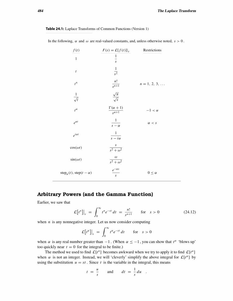
The table we will use is table 24.1, Laplace Transforms of Common Functions (Version 1), on

page 484. Checking that table, we see that we have already verified all but two or three of the

entries, with those being the transforms of fairly arbitrary powers of t , tα , and the “shifted step

function”, step(t − α) . So let’s compute them now.


Table 24.1: Laplace Transforms of Common Functions (Version 1)

In the following, α and ω are real-valued constants, and, unless otherwise noted, s > 0 .

f (t) F(s) = L[ f (t)]|s Restrictions

11

s

t1

s2

tn n!sn+1

n = 1, 2, 3, . . .

1√

t

√π

√s

tαŴ(α + 1)

sα+1−1 < α

eαt 1

s − αα < s

eiαt 1

s − iα

cos(ωt)s

s2 + ω2

sin(ωt)ω

s2 + ω2

stepα(t), step(t − α)e−αs

s0 ≤ α

Arbitrary Powers (and the Gamma Function)

Earlier, we saw that

L[

tn]∣∣s

=∫ ∞

0

tne−st dt = n!sn+1

for s > 0 (24.12)

when n is any nonnegative integer. Let us now consider computing

L[

tα]∣∣s

=∫ ∞

0

tαe−st dt for s > 0

when α is any real number greater than −1 . (When α ≤ −1 , you can show that tα ‘blows up’

too quickly near t = 0 for the integral to be finite.)

The method we used to find L[tn] becomes awkward when we try to apply it to find L[tα]

when α is not an integer. Instead, we will ‘cleverly’ simplify the above integral for L[tα] by

using the substitution u = st . Since t is the variable in the integral, this means

t = u

sand dt = 1

sdu .


So, assuming s > 0 and α > −1 ,

L[

tα]∣∣s

=∫ ∞

0

tαe−st dt

=∫ ∞

0

(u

s

)α

e−u 1

sdu

=∫ ∞

0

uα

sα+1e−u du = 1

sα+1

∫ ∞

0

uαe−u du .

Notice that the last integral depends only on the constant α — we’ve ‘factored out’ any depen-

dence on the variable s . Thus, we can treat this integral as a constant (for each value of α ) and

write

L[

tα]∣∣s

= Cα

sα+1where Cα =

∫ ∞

0

uαe−u du .

It just so happens that the above formula for Cα is very similar to the formula for something

called the “Gamma function”. This is a function that crops up in various applications (such as

this) and, for x > 0 , is given by

Ŵ(x) =∫ ∞

0

ux−1e−u du . (24.13)

Comparing this with the formula for Cα , we see that

Cα =∫ ∞

0

uαe−u du =∫ ∞

0

u(α+1)−1e−u du = Ŵ(α + 1) .

So our formula for the Laplace transform of tα (with α > −1 ) can be written as

L[

tα]∣∣s

= Ŵ(α + 1)

sα+1for s > 0 . (24.14)

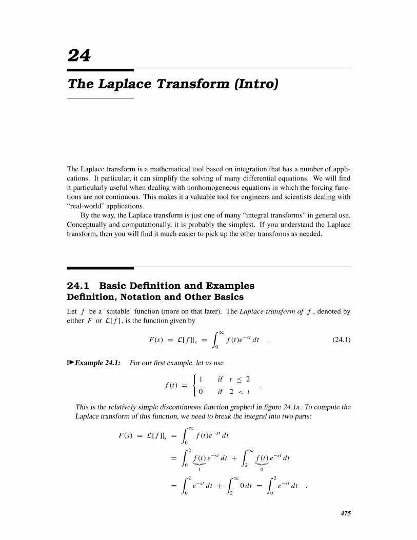
This is normally considered the preferred way to express L[tα] because the Gamma function is

considered to be a “well-known” function. Perhaps you don’t yet consider it “well known”, but

you can find tables for evaluating Ŵ(x) , and it is probably one of the functions already defined

in your favorite computer math package. That makes graphing Ŵ(x) , as done in figure 24.2,

relatively easy.

As it is, we can readily determine the value of Ŵ(x) when x is a positive integer by

comparing our two formulas for L[tn] when n is a nonnegative integer — the one mentioned

at the start of our discussion (formula (24.12)), and the more general formula (formula (24.14))

just derived for L[tα] with α = n :

n!sn+1

= L[

tn]∣∣s

= Ŵ(n + 1)

sn+1when n = 0, 1, 2, 3, 4, . . . .

Thus,

Ŵ(n + 1) = n! when n = 0, 1, 2, 3, 4, . . . .

Letting x = n + 1 , this becomes

Ŵ(x) = (x − 1)! when x = 1, 2, 3, 4, . . . . (24.15)

In particular:

Ŵ(1) = (1 − 1)! = 0! = 1 ,

Ŵ(2) = (2 − 1)! = 1! = 1 ,


X1 2 3 4

2

4

6

0

8

0

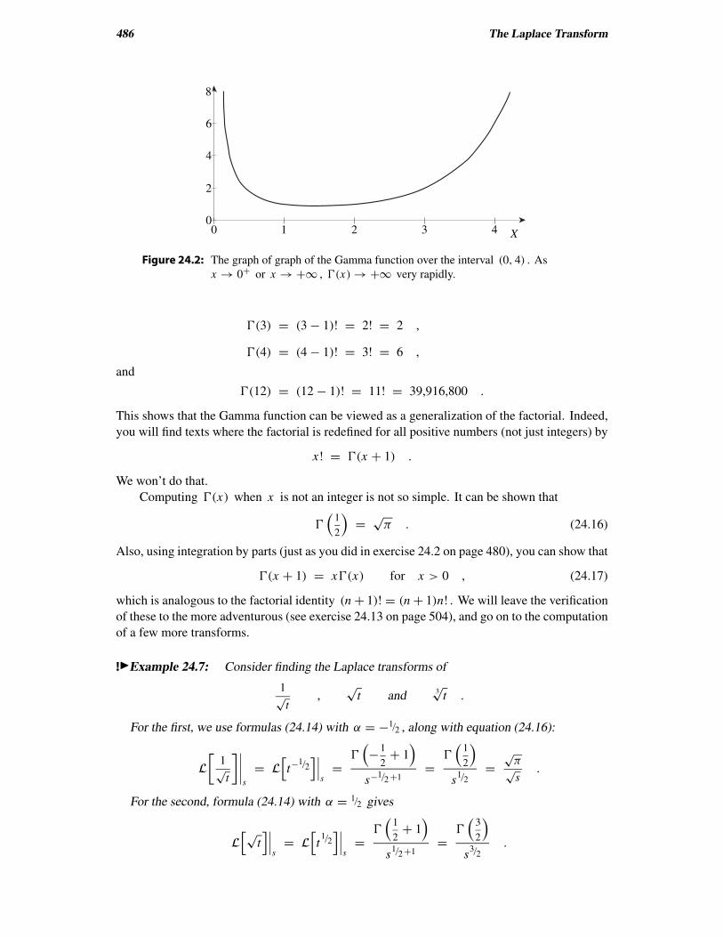
Figure 24.2: The graph of graph of the Gamma function over the interval (0, 4) . As

x → 0+ or x → +∞ , Ŵ(x) → +∞ very rapidly.

Ŵ(3) = (3 − 1)! = 2! = 2 ,

Ŵ(4) = (4 − 1)! = 3! = 6 ,

and

Ŵ(12) = (12 − 1)! = 11! = 39,916,800 .

This shows that the Gamma function can be viewed as a generalization of the factorial. Indeed,

you will find texts where the factorial is redefined for all positive numbers (not just integers) by

x ! = Ŵ(x + 1) .

We won’t do that.

Computing Ŵ(x) when x is not an integer is not so simple. It can be shown that

Ŵ(

1

2

)

=√

π . (24.16)

Also, using integration by parts (just as you did in exercise 24.2 on page 480), you can show that

Ŵ(x + 1) = xŴ(x) for x > 0 , (24.17)

which is analogous to the factorial identity (n + 1)! = (n + 1)n! . We will leave the verification

of these to the more adventurous (see exercise 24.13 on page 504), and go on to the computation

of a few more transforms.

!◮Example 24.7: Consider finding the Laplace transforms of

1√

t,

√t and

3√

t .

For the first, we use formulas (24.14) with α = −1/2 , along with equation (24.16):

L

[

1√

t

]∣∣∣∣s

= L

[

t−1/2

]∣∣∣s

=Ŵ

(

−1

2+ 1

)

s−1/2 +1=

Ŵ(

1

2

)

s1/2

=√

π√

s.

For the second, formula (24.14) with α = 1/2 gives

L

[√t]∣∣∣s

= L

[

t1/2

]∣∣∣s

=Ŵ

(1

2+ 1

)

s1/2 +1

=Ŵ

(3

2

)

s3/2

.


Using formulas (24.17) and (24.16), we see that

Ŵ(

3

2

)

= Ŵ(

1

2+ 1

)

= 1

2Ŵ

(1

2

)

= 1

2

√π .

Thus

L

[√t]∣∣∣s

= L

[

t1/2

]∣∣∣s

=Ŵ

(3

2

)

s3/2

=√

π

2s3/2

.

For the transform of 3√

t , we simply have

L

[3√

t]∣∣∣s

= L

[

t1/3

]∣∣∣s

=Ŵ

(1

3+ 1

)

s1/3 +1

=Ŵ

(4

3

)

s4/3

.

Unfortunately, there is not a formula analogous to (24.16) for Ŵ(

4/3

)

or Ŵ(

1/3

)

. There is the

approximation

Ŵ(

4

3

)

≈ .8929795121 ,

which can be found using either tables or a computer math package, but, since this is just an

approximation, we might as well leave our answer as

L

[3√

t]∣∣∣s

= L

[

t1/3

]∣∣∣s

=Ŵ

(4

3

)

s4/3

.

The Shifted Unit Step Function

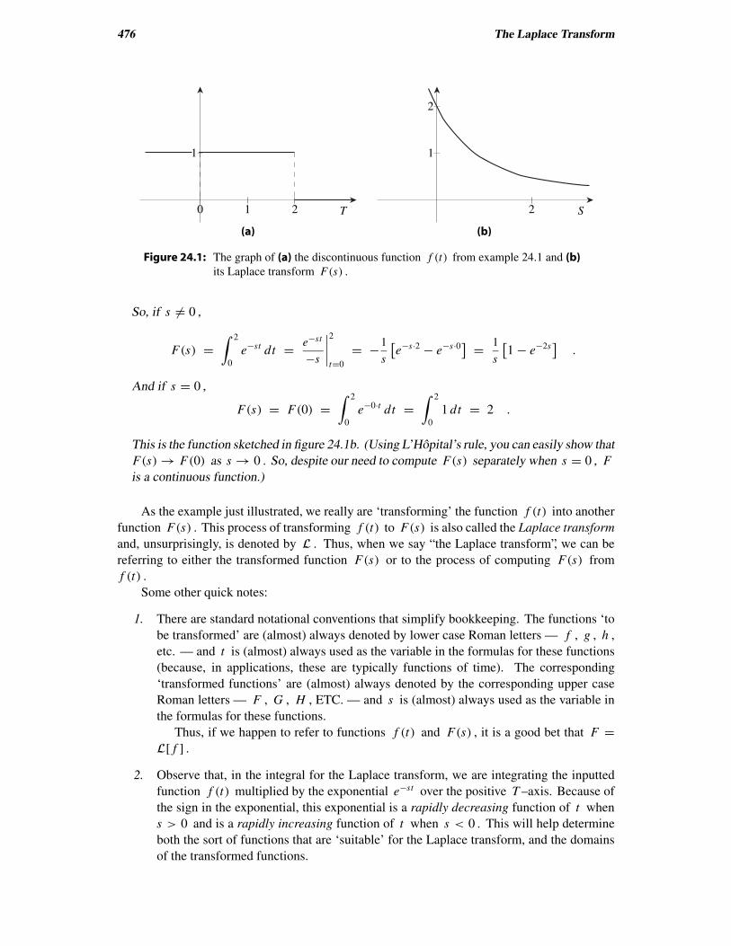
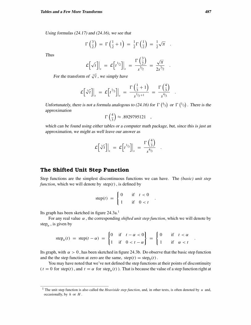
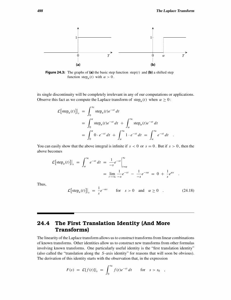
Step functions are the simplest discontinuous functions we can have. The (basic) unit step

function, which we will denote by step(t) , is defined by

step(t) =

{

0 if t < 0

1 if 0 < t.

Its graph has been sketched in figure 24.3a.1

For any real value α , the corresponding shifted unit step function, which we will denote by

stepα , is given by

stepα(t) = step(t − α) =

{

0 if t − α < 0

1 if 0 < t − α

}

=

{

0 if t < α

1 if α < t.

Its graph, with α > 0 , has been sketched in figure 24.3b. Do observe that the basic step function

and the the step function at zero are the same, step(t) = step0(t) .

You may have noted that we’ve not defined the step functions at their points of discontinuity

( t = 0 for step(t) , and t = α for stepα(t) ). That is because the value of a step function right at

1 The unit step function is also called the Heaviside step function, and, in other texts, is often denoted by u and,

occasionally, by h or H .


(a) (b)

α TT 00

11

Figure 24.3: The graphs of (a) the basic step function step(t) and (b) a shifted step

function stepα(t) with α > 0 .

its single discontinuity will be completely irrelevant in any of our computations or applications.

Observe this fact as we compute the Laplace transform of stepα(t) when α ≥ 0 :

L[

stepα(t)]∣∣s

=∫ ∞

0

stepα(t)e−st dt

=∫ α

0

stepα(t)e−st dt +

∫ ∞

α

stepα(t)e−st dt

=∫ α

0

0 · e−st dt +∫ ∞

α

1 · e−st dt =∫ ∞

α

e−st dt .

You can easily show that the above integral is infinite if s < 0 or s = 0 . But if s > 0 , then the

above becomes

L[

stepα(t)]∣∣s

=∫ ∞

α

e−st dt = 1

−se−st

∣∣∣∣

∞

t=α

= limt→∞

1

−se−st − 1

−se−sα = 0 + 1

seαs .

Thus,

L[

stepα(t)]∣∣s

= 1

se−αs for s > 0 and α ≥ 0 . (24.18)

24.4 The First Translation Identity (And MoreTransforms)

The linearity of the Laplace transform allows us to construct transforms from linear combinations

of known transforms. Other identities allow us to construct new transforms from other formulas

involving known transforms. One particularly useful identity is the “first translation identity”

(also called the “translation along the S–axis identity” for reasons that will soon be obvious).

The derivation of this identity starts with the observation that, in the expression

F(s) = L[ f (t)]|s =∫ ∞

0

f (t)e−st dt for s > s0 ,

The First Translation Identity (And More Transforms) 489

the s is simply a place holder. It can be replaced with any symbol, say, X , that does not involve

the constant of integration t ,

F(X) = L[ f (t)]|X =∫ ∞

0

f (t)e−Xt dt for X > s0 .

In particular, let X = s − α where α is any real constant. Using this for X in the above gives

us

F(s − α) = L[ f (t)]|s−α =∫ ∞

0

f (t)e−(s−α)t dt for s − α > s0 .

But

s − α > s0 ⇐⇒ s > s0 + α

and ∫ ∞

0

f (t)e−(s−α)t dt =∫ ∞

0

f (t)e−steαt dt

=∫ ∞

0

eαt f (t)e−st dt = L[

eαt f (t)]∣∣s

.

So the expression above for F(s − α) can be written as

F(s − α) = L[

eαt f (t)]∣∣s

for s > s0 + α .

This gives us the following identity:

Theorem 24.2 (First translation identity)

If

L[ f (t)]|s = F(s) for s > s0 ,

then, for any real constant α ,

L[

eαt f (t)]∣∣s

= F(s − α) for s > s0 + α . (24.19)

This is called a ‘translation identity’ because the graph of the right side of the identity,

equation (24.19), is the graph of F(s) translated to the right by α .2,3 (The second translation

identity, in which f is the function shifted, will be developed later.)

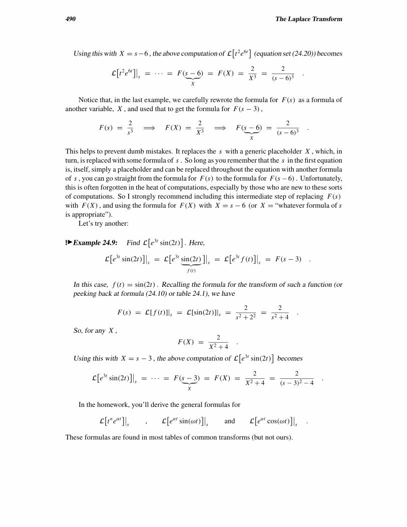
!◮Example 24.8: Let us use this translation identity to find the transform of t2e6t . First we

must identify the ‘ f (t) ’ and the ‘ α ’ and then apply the identity:

L[

t2e6t]∣∣s

= L[

e6t t2

︸︷︷︸

f (t)

]∣∣s

= L[

e6t f (t)]∣∣s

= F(s − 6) . (24.20)

Here, f (t) = t2 and α = 6 . From either formula (24.7) or table 24.1, we know

F(s) = L[ f (t)]|s = L[

t2]∣∣s

= 2!s2+1

= 2

s3.

So, for any X ,

F(X) = 2

X3.

2 More precisely, it’s shifted to the right by α if α > 0 , and is shifted to the left by |a| if α < 0 .3 Some authors prefer to use the word “shifting” instead of “translation”.


Using this with X = s−6 , the above computation of L[

t2e6t]

(equation set (24.20)) becomes

L[

t2e6t]∣∣s

= · · · = F(s − 6︸︷︷︸

X

) = F(X) = 2

X3= 2

(s − 6)3.

Notice that, in the last example, we carefully rewrote the formula for F(s) as a formula of

another variable, X , and used that to get the formula for F(s − 3) ,

F(s) = 2

s3H⇒ F(X) = 2

X3H⇒ F(s − 6

︸︷︷︸

X

) = 2

(s − 6)3.

This helps to prevent dumb mistakes. It replaces the s with a generic placeholder X , which, in

turn, is replaced with some formula of s . So long as you remember that the s in the first equation

is, itself, simply a placeholder and can be replaced throughout the equation with another formula

of s , you can go straight from the formula for F(s) to the formula for F(s −6) . Unfortunately,

this is often forgotten in the heat of computations, especially by those who are new to these sorts

of computations. So I strongly recommend including this intermediate step of replacing F(s)

with F(X) , and using the formula for F(X) with X = s − 6 (or X = “whatever formula of s

is appropriate”).

Let’s try another:

!◮Example 24.9: Find L[

e3t sin(2t)]

. Here,

L[

e3t sin(2t)]∣∣s

= L[

e3t sin(2t)︸︷︷︸

f (t)

]∣∣s

= L[

e3t f (t)]∣∣s

= F(s − 3) .

In this case, f (t) = sin(2t) . Recalling the formula for the transform of such a function (or

peeking back at formula (24.10) or table 24.1), we have

F(s) = L[ f (t)]|s = L[sin(2t)]|s = 2

s2 + 22= 2

s2 + 4.

So, for any X ,

F(X) = 2

X2 + 4.

Using this with X = s − 3 , the above computation of L[

e3t sin(2t)]

becomes

L[

e3t sin(2t)]∣∣s

= · · · = F(s − 3︸︷︷︸

X

) = F(X) = 2

X2 + 4= 2

(s − 3)2 − 4.

In the homework, you’ll derive the general formulas for

L[

tneαt]∣∣s

, L[

eαt sin(ωt)]∣∣s

and L[

eαt cos(ωt)]∣∣s

.

These formulas are found in most tables of common transforms (but not ours).

What Is “Laplace Transformable”? 491

(a) (b)

T T

Y Y

t0 t0 t1 t2

jumpmidpoint

of jump

0 0

limt→t0

+f (t)

limt→t0

−f (t)

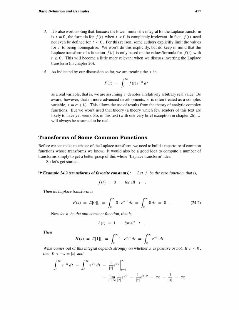
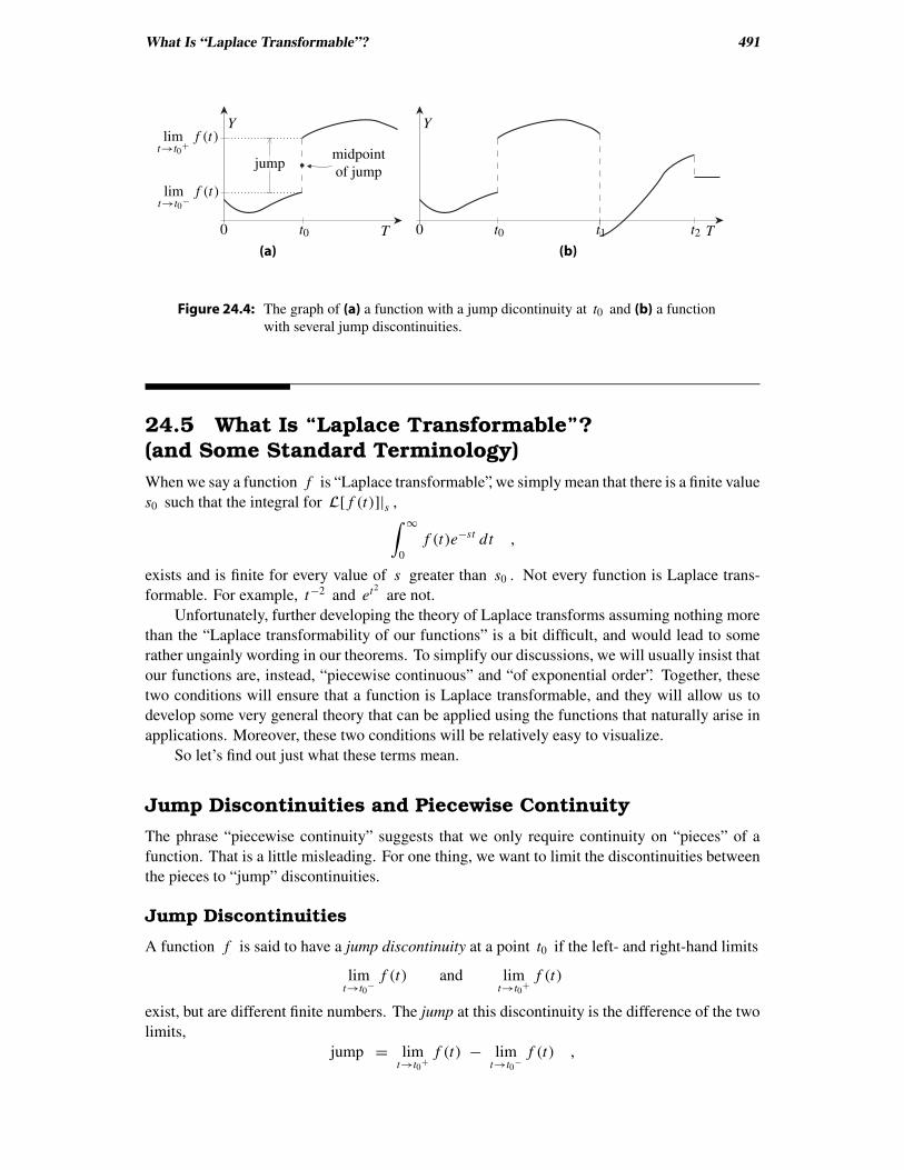
Figure 24.4: The graph of (a) a function with a jump dicontinuity at t0 and (b) a function

with several jump discontinuities.

24.5 What Is “Laplace Transformable”?(and Some Standard Terminology)

When we say a function f is “Laplace transformable”, we simply mean that there is a finite value

s0 such that the integral for L[ f (t)]|s ,∫ ∞

0

f (t)e−st dt ,

exists and is finite for every value of s greater than s0 . Not every function is Laplace trans-

formable. For example, t−2 and et2are not.

Unfortunately, further developing the theory of Laplace transforms assuming nothing more

than the “Laplace transformability of our functions” is a bit difficult, and would lead to some

rather ungainly wording in our theorems. To simplify our discussions, we will usually insist that

our functions are, instead, “piecewise continuous” and “of exponential order”. Together, these

two conditions will ensure that a function is Laplace transformable, and they will allow us to

develop some very general theory that can be applied using the functions that naturally arise in

applications. Moreover, these two conditions will be relatively easy to visualize.

So let’s find out just what these terms mean.

Jump Discontinuities and Piecewise Continuity

The phrase “piecewise continuity” suggests that we only require continuity on “pieces” of a

function. That is a little misleading. For one thing, we want to limit the discontinuities between

the pieces to “jump” discontinuities.

Jump Discontinuities

A function f is said to have a jump discontinuity at a point t0 if the left- and right-hand limits

limt→t0

−f (t) and lim

t→t0+

f (t)

exist, but are different finite numbers. The jump at this discontinuity is the difference of the two

limits,

jump = limt→t0

+f (t) − lim

t→t0−

f (t) ,


(a) (b) (c)

T TT

Y Y Y

2 2

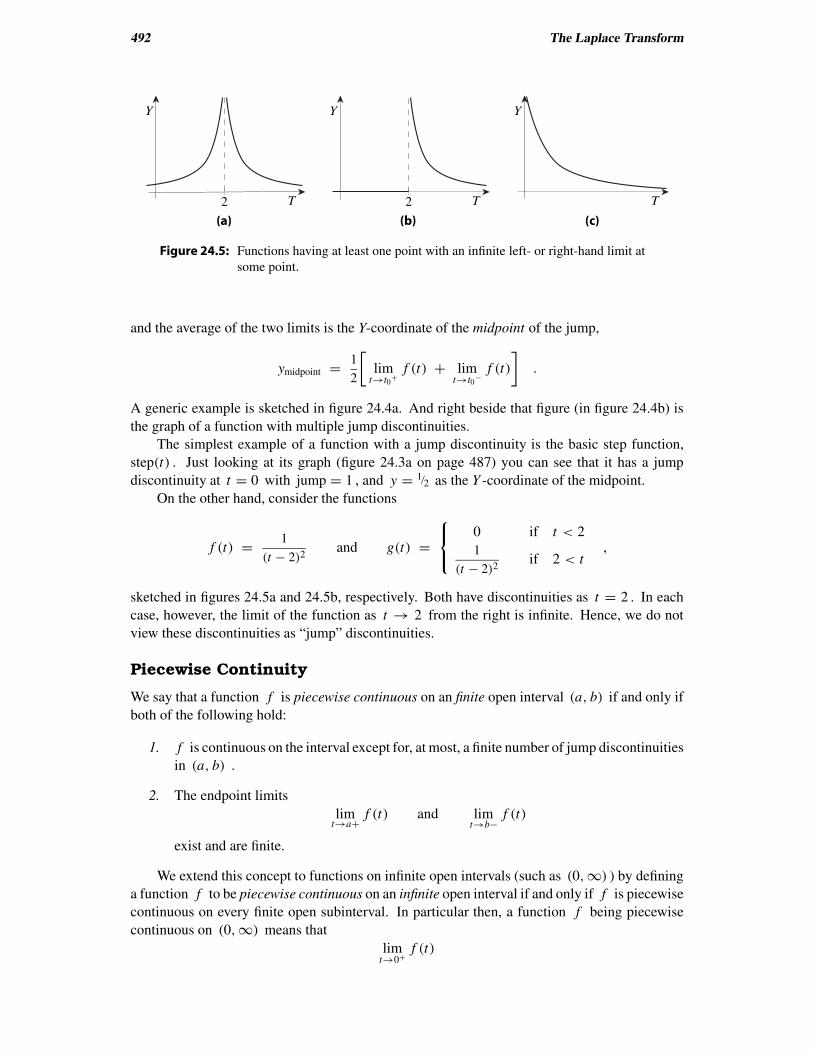
Figure 24.5: Functions having at least one point with an infinite left- or right-hand limit at

some point.

and the average of the two limits is the Y-coordinate of the midpoint of the jump,

ymidpoint = 1

2

[

limt→t0

+f (t) + lim

t→t0−

f (t)

]

.

A generic example is sketched in figure 24.4a. And right beside that figure (in figure 24.4b) is

the graph of a function with multiple jump discontinuities.

The simplest example of a function with a jump discontinuity is the basic step function,

step(t) . Just looking at its graph (figure 24.3a on page 487) you can see that it has a jump

discontinuity at t = 0 with jump = 1 , and y = 1/2 as the Y -coordinate of the midpoint.

On the other hand, consider the functions

f (t) = 1

(t − 2)2and g(t) =

0 if t < 2

1

(t − 2)2if 2 < t

,

sketched in figures 24.5a and 24.5b, respectively. Both have discontinuities as t = 2 . In each

case, however, the limit of the function as t → 2 from the right is infinite. Hence, we do not

view these discontinuities as “jump” discontinuities.

Piecewise Continuity

We say that a function f is piecewise continuous on an finite open interval (a, b) if and only if

both of the following hold:

1. f is continuous on the interval except for, at most, a finite number of jump discontinuities

in (a, b) .

2. The endpoint limits

limt→a+

f (t) and limt→b−

f (t)

exist and are finite.

We extend this concept to functions on infinite open intervals (such as (0,∞) ) by defining

a function f to be piecewise continuous on an infinite open interval if and only if f is piecewise

continuous on every finite open subinterval. In particular then, a function f being piecewise

continuous on (0,∞) means that

limt→0+

f (t)


is a finite value, and that, for every finite, positive value T , f (t) has at most a finite number of

discontinuities on the interval (0, T ) , with each of those being a jump discontinuity.

For some of our discussions, we will only need our function f to be piecewise continuous

on (0,∞) . Strictly speaking, this says nothing about the possible value of f (t) when t = 0 .

If, however, we are dealing with initial-value problems, then we may require our function f to

be piecewise continuous on [0,∞) , which simply means f is piecewise continuous on (0,∞) ,

defined at t = 0 , and

f (0) = limt→0+

f (t) .

Keep in mind that “a finite number” of jump discontinuities can be zero, in which case

f has no discontinuities and is, in fact, continuous on that interval. What is important is that

a piecewise continuous function cannot ‘blow up’ at any (finite) point in or at the ends of the

interval. At worst, it has only ‘a few’ jump discontinuities in each finite subinterval.

The functions sketched in figure 24.4 are piecewise continuous, at least over the intervals in

the figures. And any step function is piecewise continuous on (0,∞) . On the other hand, the

functions sketched in figures 24.5a and 24.5b, are not piecewise continuous on (0,∞) because

they both “blow up” at t = 2 . Consider even the function

f (t) = 1

t,

sketched in figure 24.5c. Even though this function is continuous on the interval (0,∞) , we do

not consider it to be piecewise continuous on (0,∞) because

limt→0+

1

t= ∞ .

Two simple observations will soon be important to us:

1. If f is piecewise continuous on (0,∞) , and T is any positive finite value, then the

integral∫ T

0

f (t) dt

is well defined and evaluates to a finite number. Remember, geometrically, this integral

is the “net area” between the graph of f and the T –axis over the interval (0, T ) . The

piecewise continuity of f assures us that f does not “blow up” at any point in (0, T ) ,

and that we can divide the graph of f over (0, T ) into a finite number of fairly nicely

behaved ‘pieces’ (see figure 24.4b) with each piece enclosing finite area.

2. The product of any two piecewise continuous functions f and g on (0,∞) will, itself,

be piecewise continuous on (0,∞) . You can easily verify this yourself using the fact

that

limt→t0

±f (t)g(t) = lim

t→t0±

f (t) × limt→t0

±g(t) .

Combining the above two observations with the obvious fact that, for any real value of s ,

g(t) = e−st is a piecewise continuous function of t on (0,∞) gives us:


Lemma 24.3

Let f be a piecewise continuous function on (0,∞) , and let T be any finite positive number.

Then the integral∫ T

0

f (t)e−st dt

is a well-defined finite number for each real value s .

Because of our interest in the Laplace transform, we will want to ensure that the above

integral converges to a finite number as T → ∞ . That is the next issue we will address.

Exponential Order∗

Let f be a function on (0,∞) , and let s0 be some real number. We say that f is of exponential

order s0 if and only if there are finite constants M and T such that

| f (t)| ≤ Mes0t whenever T ≤ t . (24.21)

Often, the precise value of s0 is not particularly important. In these cases we may just say that

f is of exponential order to indicate that it is of exponential order s0 for some value s0 .

Saying that f is of exponential order is just saying that the graph of | f (t)| is bounded

above by the graph of some constant multiple of some exponential function on some interval of

the form [T,∞) . Note that, if this is the case and s is any real number, then∣∣ f (t)e−st

∣∣ = | f (t)| e−st ≤ Mes0t e−st = Me−(s−s0)t whenever T ≤ t .

Moreover, if s > s0 , then s − s0 is positive, and∣∣ f (t)e−st

∣∣ ≤ Me−(s−s0)t → 0 as t → ∞ . (24.22)

Thus, in the future, we will automatically know that

limt→∞

f (t)e−st = 0

whenever f is of exponential order s0 and s > s0 .

Transforms of Piecewise Continuous Functions ofExponential Order

Now, suppose f is a piecewise continuous function of exponential order s0 on the interval

(0,∞) . As already observed, the piecewise continuity of f assures us that

∫ T

0

f (t)e−st dt

is a well-defined finite number for each T > 0 . And if s > s0 , then inequality (24.22), above,

tells us that f (t)e−st is shrinking to 0 as t → ∞ at least as fast as a constant multiple of some

decreasing exponential. It is easy to verify that this is fast enough to ensure that

limT →∞

∫ T

0

f (t)e−st dt

∗ More precisely: Exponential Order as t → ∞ . One can have “exponential order as t → −∞ ” and even “as

t → 3 ”). However, we are not interested in those cases, and it is silly to keep repeating “as t → ∞ ”.


converges to some finite value. And that gives us the following theorem on conditions ensuring

the existence of Laplace transforms.

Theorem 24.4

If f is both piecewise continuous on (0,∞) and of exponential order s0 , then

F(s) = L[ f (t)]|s =∫ ∞

0

f (t)e−st dt

is a well-defined function for s > s0 .

In the next several chapters, we will often assume that our functions of t are both piecewise

continuous on (0,∞) and of exponential order. Mind you, not all Laplace transformable func-

tions satisfy these conditions. For example, we’ve already seen that tα with −1 < α is Laplace

transformable. But

limt→0+

tα = ∞ if α < 0 .

So those functions given by tα with −1 < α < 0 (such as 1/√t ) are not not piecewise continuous

on (0,∞) , even though they are certainly Laplace transformable. Still, all the other functions on

the left side of table 24.1 on page 484 are piecewise continuous on (0,∞) and are of exponential

order. More importantly, the functions that naturally arise in applications in which the Laplace

transform may be useful are usually piecewise continuous on (0,∞) and of exponential order.

By the way, since you’ve probably just glanced at table 24.1 on page 484, go back at look

at the functions on the right side of the table. Observe that

1. these functions have no discontinuities in the intervals on which they are defined,

and

2. they all shrink to 0 as s → ∞ .

It turns out that you can extend the work used to obtain the above theorem to show that the above

observations hold much more generally. More precisely, the above theorem can be extended to:

Theorem 24.5

If f is both piecewise continuous on (0,∞) and of exponential order s0 , then

F(s) = L[ f (t)]|s =∫ ∞

0

f (t)e−st dt

is a continuous function on (s0,∞) and

lims→∞

F(s) = 0 .

We will verify this theorem at the end of the next section.


24.6 Further Notes on Piecewise Continuous andExponentially Bounded Functions

Issues Regarding Piecewise Continuous Functions on (0, ∞)

In the next several chapters, we will be concerned mainly with functions that are piecewise

continuous on (0,∞) . There are a few small technical issues regarding these functions that

could become significant later if we don’t deal with them now. These issues concern the values

of such functions at jumps.

On the Value of a Function at a Jump

Take a look at figure 24.4b on page 491. Call the function sketched there f , and consider

evaluating, say,∫ t2

0

f (t)e−st dt .

The obvious approach is to break up the integral into three pieces,

∫ t2

0

f (t)e−st dt =∫ t0

0

f (t)e−st dt +∫ t1

t0

f (t)e−st dt +∫ t2

t1

f (t)e−st dt ,

and use values/formulas for f over the intervals (0, t0) , (t0, t1) and (t1, t2) to compute the

individual integrals in the above sum. What you would not worry about would be the actual

values of f at the points of discontinuity, t0 , t1 and t2 . In particular, it would not matter if

f (t0) = limt→t0

−f (t) or f (t0) = lim

t→t0+

f (t)

or

f (t0) = the Y-coordinate of the midpoint of the jump .

This extends an observation made when we computed the Laplace transform of the shifted

step function. There, we found that the precise value of stepα(t) at t = α was irrelevant to the

computation of L[

stepα(t)]

. And the pseudo-computations in the previous paragraph point out

that, in general, the value of any piecewise continuous function at a point of discontinuity will

be irrelevant to the integral computations we will be doing with these functions.

Parallel to these observations are the observations of how we use functions with jump

discontinuities in applications. Typically, a function with a jump discontinuity at t = t0 is

modeling something that changes so quickly around t = t0 that we might as well pretend the

change is instantaneous. Consider, for example, the output of a one-lumen incandescent light

bulb switched on at t = 2 : Until is is switched on, the bulb’s light output is 0 lumen. For a

brief period around t = 2 the filament is warming up and the light output increases from 0 to

1 lumen, and remains at 1 lumen thereafter. In practice, however, the warm-up time is so brief

that we don’t notice it, and are content to describe the light output by

light output at time t =

{

0 lumen if t < 2

1 lumen if 2 < t

}

= step2(t) lumen

Notes on Piecewise Continuous and Exponentially Bounded Functions 497

without giving any real thought as to the value of the light output the very instant we are turning

on the bulb.4

What all this is getting to is that, for our work involving piecewise continuous functions on

(0,∞) ,

the value of a function f at any point of discontinuity t0 in (0,∞) is irrelevant.

What is important is not f (t0) but the one-sided limits

limt→t0

−f (t) and lim

t→t0+

f (t) .

Because of this, we will not normally specify the value of a function at a discontinuity, at

least not while developing Laplace transforms. If this disturbs you, go ahead and assume that,

unless otherwise indicated, the value of a function at each jump discontinuity is given by the

Y -coordinate of the jump’s midpoint. It’s as good as any other value.

Equality of Piecewise Continuous Functions

Because of the irrelevance of the value of a function at a discontinuity, we need to slightly modify

what it means to say “ f = g on some interval”. Henceforth, let us say that

f = g on some interval (as piecewise continuous functions)

means

f (t) = g(t)

for every t in the interval at which f and g are continuous. We will not insist that f and g

be equal at the relatively few points of discontinuity in the functions. But do note that we will

still have

limt→t0

±f (t) = lim

t→t0±

g(t)

for every t0 in the interval. Consequently, the graphs of f and g will have the same ‘jumps’

in the interval.

By the way, the phrase “as piecewise continuous functions” in the above definition is rec-

ommended, but is often forgotten.

!◮Example 24.10: The functions

step2(t) , f (t) =

{

0 if t ≤ 2

1 if 2 < tand g(t) =

{

0 if t < 2

1 if 2 ≤ t

all satisfy

step2(t) = f (t) = g(t)

for all values of t in (0,∞) except t = 2 , at which each has a jump. So, as piecewise

continuous functions,

step2 = f = g on (0,∞) .

4 On the other hand, “What is the light output of a one-lumen light bulb the very instant the light is turned on?” is a

nice question to meditate upon if you are studying Zen.


Conversely, if we know h = step2 on (0,∞) (as piecewise continuous functions), then

we know

h(t) =

{

0 if 0 < t < 2

1 if 2 < t.

We do not know (nor do we care about) the value of h(t) when t = 2 (or when t < 0 ).

Testing for Exponential Order

Before deriving this test for exponential order, it should be noted that the “order” is not unique.

After all, if

| f (t)| ≤ Mes0t whenever T ≤ t ,

and s0 ≤ s1 , then

| f (t)| ≤ Mes0t ≤ Mes1t whenever T ≤ t ,

proving the following little lemma:

Lemma 24.6

If f is of exponential order s0 , then f is of exponential order s1 for every s1 ≥ s0 .

Now here is the test:

Lemma 24.7 (test for exponential order)

Let f be a function on (0,∞) .

1. If there is a real value s0 such that

limt→∞

f (t)e−s0t = 0 ,

then f is of exponential order s0 .

2. If

limt→∞

f (t)e−st

does not converge to 0 for any real value s , then f is not of exponential order.

PROOF: First, assume

limt→∞

f (t)e−s0t = 0

for some real value s0 , and let M be any finite positive number you wish (it could be 1 , 1/2 ,

827 , whatever). By the definition of “limits”, the above assures us that, if t is large enough, then

f (t)e−s0t is within M of 0 . Letting T be any single “large enough” value of t , we then must

have

t ≥ T H⇒∣∣ f (t)e−s0t − 0

∣∣ ≤ M .

By elementary algebra, we can rewrite this as

| f (t)| ≤ Mes0t whenever T ≤ t ,


which is exactly what we mean when we say “ f is of exponential order s0 ”. That confirms the

first part of the lemma.

To verify the second part of the lemma, assume

limt→∞

f (t)e−st

does not converge to 0 for any real value s . If f were of exponential order, then it is of

exponential order s0 for some finite real number s0 , and, as noted in the discussion of expression

(24.22) on page 494, we would then have that

limt→∞

f (t)e−st = 0 for s > s0 .

But we’ve assumed this is not possible; thus, it is not possible for f to be of exponential order.

Proving Theorem 24.5The Theorem and a Bad Proof

The basic premise of theorem 24.5 is that we have a piecewise continuous function f on (0,∞)

which is also of exponential order s0 . From the previous theorem, we know

F(s) = L[ f (t)]|s =∫ ∞

0

f (t)e−st dt

is a well-defined function on (s0,∞) . Theorem 24.5 further claims that

1. F(s) = L[ f (t)]|s is continuous on (s0,∞) . That is,

lims→s1

F(s) = F(s1) for each s1 > s0 .

and

2. lims→∞

F(s) = 0 .

In a naive attempt to verify these claims, you might try

lims→s1

F(s) = lims→s1

∫ ∞

0

f (t)e−st dt

=∫ ∞

0

lims→s1

f (t)e−st dt =∫ ∞

0

f (t)e−s1t dt = F(s1) ,

and

lims→∞

F(s) = lims→∞

∫ ∞

0

f (t)e−st dt

=∫ ∞

0

lims→∞

f (t)e−st dt =∫ ∞

0

f (t) · 0 dt = 0 .

Unfortunately, these computations assume

lims→α

∫ ∞

0

g(t, s) dt =∫ ∞

0

lims→α

g(t, s) dt

which is NOT always true. Admittedly, it often is true. But there are exceptions. And because

there are exceptions, we cannot rely on this sort of “switching of limits with integrals” to prove

our claims.


Preliminaries

There are two small observations that will prove helpful here and elsewhere.

The first concerns any function f which is piecewise continuous on (0,∞) and satisfies

| f (t)| ≤ MT es0t whenever T ≤ t ,

for two positive values MT and T . For convenience, let

g(t) = f (t)e−s0t for t > 0 .

This is another piecewise continuous function on (0,∞) , but it satisfies

|g(t)| =∣∣ f (t)e−s0t

∣∣ = | f (t)| e−s0t ≤ Mes0te−s0t = M for T < t ,

On the other hand, the piecewise continuity of g on (0,∞) means that g does not “blow up”

anywhere in or at the endpoints of (0, T ) . So it is easy to see (and to prove) that there is a

constant B such that

|g(t)| ≤ B for 0 < t < T .

Letting M0 be the larger of B and MT , we now have that

|g(t)| ≤ M0 if 0 < t < T or T ≤ t .

So,

| f (t)| e−s0t =∣∣ f (t)e−s0t

∣∣ = |g(t)| ≤ M0 for 0 < t .

Multiply through by the exponential, and you’ve got:

Lemma 24.8

Assume f is a piecewise continuous function on (0,∞) which is also of exponential order s0 .

Then there is a constant M0 such that

| f (t)| ≤ M0es0t for 0 < t .

The above lemma will let us use the exponential bound M0es0t over all of (0,∞) , and not

just (MT ,∞) . The next lemma is one you should either already be acquainted with, or can

easily confirm on your own.

Lemma 24.9

If g is an integrable function on the interval (a, b) , then

∣∣∣∣

∫ b

a

g(t) dt

∣∣∣∣

≤∫ b

a

|g(t)| dt .


The Proof of Theorem 24.5

Now we will prove the two claims of theorem 24.5. Keep in mind that f is a piecewise continuous

function on (0,∞) of exponential order s0 , and that

F(s) =∫ ∞

0

f (t)e−st dt for s > s0 .

We will make repeated use of the fact, stated in lemma 24.8 just above, that there is a constant

M0 such that

| f (t)| ≤ M0es0t for 0 < t . (24.23)

Since the second claim is a little easier to verify, we will start with that.

Proof of the Second Claim

The second claim is that

lims→∞

F(s) = 0 ,

which, of course, can be proven by showing

lims→∞

|F(s)| ≤ 0 .

Now let s > s0 . Using inequality (24.23) with the integral inequality form lemma 24.9, we

have

|F(s)| =∣∣∣∣

∫ ∞

0

f (t)e−st dt

∣∣∣∣

≤∫ ∞

0

∣∣ f (t)e−st

∣∣ dt

=∫ ∞

0

| f (t)| e−st dt

≤∫ ∞

0

M0es0t e−st dt = M0L[

es0t]∣∣s

= M0

s − s0

.

Thus,

lims→∞

|F(s)| ≤ lims→∞

M0

s − s0

= 0 ,

confirming the claim.

Proof of the First Claim

The first claim is that F is continuous on (s0,∞) . To prove this, we need to show that, for each

s1 > s0 ,

lims→s1

F(s) = F(s1) .

Note that this limit can be verified by showing

lims→s1

|F(s) − F(s1)| ≤ 0 .


Now let s and s1 be two different points in (s0,∞) . Again using inequality (24.23) with

the integral inequality from lemma 24.9,

|F(s) − F(s1)| =∣∣∣∣

∫ ∞

0

f (t)e−st dt −∫ ∞

0

f (t)e−s1t dt

∣∣∣∣

=∣∣∣∣

∫ ∞

0

f (t)[

e−st − e−s1t]

dt

∣∣∣∣

≤∫ ∞

0

| f (t)|∣∣e−st − e−s1t

∣∣ dt ≤

∫ ∞

0

M0es0t∣∣e−st − e−s1t

∣∣ dt

Observe that

∣∣e−st − e−s1t

∣∣ =

{

+[

e−st − e−s1t]

if s < s1

−[

e−st − e−s1t]

if s1 < s

}

= ±[

e−st − e−s1t]

with the sign chosen appropriately. Using this with the preceding sequence of inequalities, we

get

|F(s) − F(s1)| ≤∫ ∞

0

M0es0t∣∣e−st − e−s1t

∣∣ dt

≤ ±M0

∫ ∞

0

M0es0t[

e−st − e−s1t]

dt

≤ ±M0

[∫ ∞

0

es0t e−st dt −∫ ∞

0

es0t e−s1t dt

]

≤ ±M0

[

L[

es0t]∣∣s− L

[

es0t]∣∣s1

]

≤ ±M0

[

1

s0 − s− 1

s0 − s1

]

.

Thus,

lims→s1

|F(s) − F(s1)| ≤ lims→s1

±M0

[

1

s0 − s− 1

s0 − s1

]

= ±M0

[

1

s0 − s1

− 1

s0 − s1

]

= 0 ,

which is all we needed to show to confirm the first claim.

Additional Exercises

24.6. Sketch the graph of each of the following choices of f (t) , and then find that function’s

Laplace transform by direct application of the definition, formula (24.1) on page 475

(i.e., compute the integral). Also, if there is a restriction on the values of s for which

the formula of the transform is valid, state that restriction.

a. f (t) = 4 b. f (t) = 3e2t

c. f (t) =

{

2 if t ≤ 3

0 if 3 < td. f (t) =

{

0 if t ≤ 3

2 if 3 < t

Additional Exercises 503

e. f (t) =

{

e2t if t ≤ 4

0 if 4 < tf. f (t) =

{

e2t if 1 < t ≤ 4

0 otherwise

g. f (t) =

{

t if 0 < t ≤ 1

0 otherwiseh. f (t) =

{

0 if 0 < t ≤ 1

t otherwise

24.7. Find the Laplace transform of each, using either formula (24.7) on page 480, formula

(24.9) on page 481 or formula (24.4) on page 481, as appropriate:

a. t4 b. t9 c. e7t d. e−7t e. ei7t

24.8. Find the Laplace transform of each of the following, using table 24.1 on page 484

(Transforms of Common Functions) and the linearity of the Laplace transform:

a. sin(3t) b. cos(3t) c. 7

d. cosh(3t) e. sinh(4t) f. 3t2 − 8t + 47

g. 6e2t + 8e−3t h. 3 cos(2t) + 4 sin(6t) i. 3 cos(2t) − 4 sin(2t)

24.9. Compute the following Laplace transforms:

a. t3/2 b. t

5/2 c. t−1/3 d.4√

t e. step2(t)

24.10. For the following, let

f (t) =

{

1 if t < 2

0 if 2 ≤ t.

a. Verify that f (t) = 1 − step2(t) , and using this and linearity,

b. compute L[ f (t)]|s .

24.11. Find the Laplace transform of each of the following, using table 24.1 on page 484

(Transforms of Common Functions) and the first translation identity:

a. te4t b. t4et c. e2t sin(3t)

d. e2t cos(3t) e. e3t√

t f. e3t step2(t)

24.12. Verify each of the following using table 24.1 on page 484 (Transforms of Common

Functions) and the first translation identity (assume α and ω are real-valued constants

and n is a positive integer):

a. L[

tneαt]∣∣s

= n!(s − α)n+1

for s > α

b. L[

eαt sin(ωt)]∣∣s

= ω

(s − α)2 + ω2for s > α

c. L[

eαt cos(ωt)]∣∣s

= s − α

(s − α)2 + ω2for s > α

d. L[

eαt stepω(t)]∣∣s

= 1

s − αe−ω(s−α) for s > α and ω ≥ 0


24.13. The following problems all concern the Gamma function,

Ŵ(σ) =∫ ∞

0

e−uuσ−1 du .

a. Using integration by parts, show that Ŵ(σ + 1) = σŴ(σ) whenever σ > 0 .

b i. By using an appropriate change of variables and symmetry, verify that

Ŵ(

1

2

)

=∫ ∞

−∞e−τ 2

dτ .

ii. Starting with the observation that, by the above,

Ŵ(

1

2

)

Ŵ(

1

2

)

=(∫ ∞

−∞e−x2

dx

)(∫ ∞

−∞e−y2

dy

)

=∫ ∞

−∞

∫ ∞

−∞e−x2−y2

dx dy ,

show that

Ŵ(

1

2

)

=√

π .

(Hint: Use polar coordinates to integrate the double integral.)

24.14. Several functions are given below. Sketch the graph of each over an appropriate interval,

and decided whether each is or is not piecewise continuous on (0,∞) .

a. f (t) = 2 step3(t) b. g(t) = step2(t) − step3(t)

c. sin(t) d.sin(t

t

e. tan(t) f.√

t

g.1

√t

h. t2 − 1

i.1

t2 − 1j.

1

t2 + 1

k. The “ever increasing stair” function,

stair(t) =

0 if t < 0

1 if 0 < t < 1

2 if 2 < t < 3

3 if 3 < t < 4

4 if 4 < t < 5

......

24.15. Assume f and g are two piecewise continuous functions on an interval (a, b) con-

taining the point t0 . Assume further that f has a jump discontinuity at t0 while g is

continuous at t0 . Verify that the jump in the product f g at t0 is given by

“the jump in f at t0 ” × g(t0) .

Additional Exercises 505

24.16. Using the test for exponential order (lemma 24.7 on page 498), determine which of

the following are of exponential order, and, for each which is of exponential order,

determine the possible values for the order.

a. e3t b. t2 c. te3t

d. et2

e. sin(t)

24.17. For the following, let α and σ be any two positive numbers.

a. Using basic calculus, show that tαe−σ t has a maximum value Mα,σ on the interval

[0,∞) . Also, find both where this maximum occurs and the value of Mα,σ .

b. Explain why this confirms that

i. tα ≤ Mα,σ eσ t whenever t > 0 , and that

ii. tα is of exponential order σ for any σ > 0 .

24.18. Assume f is a piecewise continuous function on (0,∞) of exponential order s0 , and

let α and σ be any two positive numbers. Using the results of the last exercise, show

that tα f (t) is piecewise continuous on (0,∞) and of exponential order s0 + σ .

Documents

The Laplace Transform (Intro)howellkb.uah.edu/public_html/DEtext/Part4/Laplace1.pdf · The Laplace Transform (Intro) The Laplace transform is a mathematical tool based on integration