The kinks of financial journalism∗

Diego Garcıa†

Kenan-Flagler Business School

University of North Carolina at Chapel Hill

June 18, 2015

ABSTRACT

This paper studies the content of financial news as a function of past market returns. As

a proxy for media content we use positive and negative word counts from general financial

news columns from the Wall Street Journal and the New York Times. Our empirical analysis

allows us to discriminate between theories that predict hyping good stock performance to

those that emphasize negative news. The evidence is conclusive: negative market returns

taint the ink of typewriters, while positive returns barely do. Given how pervasive our

estimates are across multiple time periods, subject to different competitive pressures in the

market for news, we interpret our results as driven by demand preferences of investors.

JEL classification: G01, G14.

Keywords: media content, stock returns, journalism.

∗I would like to thank Paolo Fulghieri, David Hirshleifer, Camelia Kuhnen, Geoff Tate and seminar participantsat UNC at Chapel Hill, the University of Utah, the University of Luxembourg, Cheung Kong Graduate School ofBusiness, the Shanghai Advanced Institute of Finance, the University of California at Irvine, the Tuck School ofBusiness, and the UC Davis Symposium on information and asset prices for comments on an early draft.†Kenan-Flagler Business School, University of North Carolina at Chapel Hill, McColl Building, C.B. 3490,

Chapel Hill, NC, 27599-3490. Tel: 1-919-962-8404; Fax: 1-919-962-2068; Email:diego garcia@unc.edu; Webpage: http://www.unc.edu/∼garciadi

1 Introduction

Financial markets have permeated investors’ daily lives since the advent of newspapers.

Columns with business news, with commodity and stock price movements and commentary

around them, have been a staple in journalism virtually since the invention of the printing

press.1 This paper studies the content of a large set of columns on general finance news from

the New York Times and the Wall Street Journal for the time period 1905–2005. These columns

covered general financial news, from general stock market trends, to macroeconomic events and

discussions on individual companies. They were published every day throughout our sample,

generating a textual corpus that is quite homogeneous, and, as such, it is a nice laboratory

where to study how journalists colored different economic events for their readers.

Our empirical approach models media content by the fraction of positive and negative words

used by journalists (Tetlock, 2007) as a function of market returns over the recent past. Clearly,

DJIA returns are excellent predictors of journalists’ word choices in our columns: higher market

returns lead to journalists using more positive words, and less negative words. A parsimonious

model with only lagged market returns can explain more than 30% of the variation in media

content. More importantly, the effect is highly non-linear: positive returns have a much smaller

impact on content than negative returns. This effect is even more pronounced for lagged returns

that occurred days before the writing of the article: past returns only influence media content

when they are negative.

Our results suggest that the “hyping” in Shiller (2000) cannot generally be associated with

high market performance. On the contrary, it is the negative domain that seems to excite the

imagination of journalists. The evidence is consistent with models of human behavior where the

domain of gains and losses trigger different reactions by agents. This asymmetry corroborates

one of the main tenants of behavioral economics, the loss-aversion of Kahneman and Tversky

(1979)’s prospect theory, as well as laboratory studies on the different perceived stimuli in the

1For example, the “Notizie scritte,” first published by the government of Venezia in 1556, or “Relation,” releasedin 1605, both included economic news. Daily newspapers, very close to what we have today, were published widelyin the United Kingdom and continental Europe by the 18th century. The Economist was founded in 1843, whereasThe Financial Times and The Wall Street Journal were founded in 1888 and 1889 respectively.

1

domain of gains versus losses (Kuhnen, 2014).

The competition in the market for financial news was quite limited during most of the

20th century. Most investors only had access to a few sources for information on Wall Street,

among them the two leading newspapers we study. But our sample includes the period starting

in the 1980s, where CNN, followed by CNBC, and later the Internet cut into the turf of the

more traditional print media. Thus, we can exploit time-series variation in the supply side

of the market to see how competition affected the way journalists slanted financial news for

investors. We show the non-linearities we uncover are pervasive throughout our sample period.

The evidence from the later 25 years of our sample (1980–2005), where the supply of information

increased significantly, exhibits the same pattern as in the 1920s (or the 1950s). Furthermore,

even when conditioning on the author of the column under consideration, we find consistent

emphasis on negative news. Given the larger changes in the media landscape that occurred

throughout sample, and the idiosyncrasies of authors’ writing styles,2 we conclude that our

results are more likely to be driven by demand-side considerations (Mullainathan and Shleifer,

2005).

One can consider our empirical study a nice laboratory where to look at impulse-response “in

the field.” In contrast to other type of news (i.e., politics), the sources of discussion in our articles

(stock price movements, earnings, macroeconomic announcements) are easily measurable, and

by and large, they are continuous variables, i.e. DJIA returns. The columns we study are colored

around such variables, which gives us a particularly sharp test of the impulse response function

from stimuli (market conditions) to the printed page. The sources we include in our analysis

were the leading media providers of financial news in the United States for the majority of our

sample period, and, as such, provide a particularly nice setting in which to study how journalists

chose to slant the facts from financial markets for their readers.

Most of the literature studying the media in economics has focused on political news, and in

particular their bias towards Republicans or Democrats.3 For example, Gentzkow and Shapiro

2Dougal, Engelberg, Garcıa, and Parsons (2012) document large differences in writing style, in terms of words-per-sentence, complexity of the text, as well as unconditional pessimism.

3See DellaVigna and Gentzkow (2010) for a survey on empirical studies on persuasive communication, whichdiscusses literature from marketing, psychology and sociology as well. The survey by Prat and Stromberg (2011)

2

(2010) construct a metric of media slant based on the language used by media outlets, and

argue that reader’s preferences in the political spectrum are the key drivers of the newspapers’

slant.4 Our paper contributes to this literature by considering a very different type of slanting,

in which journalists have a continuous (multi-dimensional) variable to convey to their readers,

rather than a dichotomous (left-right) choice. As in politics, our evidence suggests demand-side

considerations are more important than supply-side variation.

Starting with Shiller (2000), financial economists have studied the effect of the media on

equilibrium outcomes. The focus of these papers is on the effect of the media on asset prices

(Tetlock, 2007; Fang and Peress, 2009), trading behavior (Barber and Odean, 2008; Engelberg

and Parsons, 2011), corporate governance (Dyck, Volchkova, and Zingales, 2008), merger nego-

tiations (Ahern and Sosyura, 2014), and IPO returns (Hanley and Hoberg, 2012; Loughran and

McDonald, 2013).5 In contrast, our paper focuses on the drivers of the media content itself, i.e.,

on the effect of asset prices and corporate events on what journalists choose to write about. A

subset of these papers study predictors of media content mostly in order to create instruments to

argue causality in a second stage.6 Finally, there is another literature that argues how advertis-

ing revenues can affect the slant and coverage of the media. For example, Reuter and Zitzewitz

(2006) show how past advertising influences mutual fund recommendations in personal finance

publications. Ellman and Germano (2009) study how such economic ties can generate biases

even in the presence of competition.

In the journalism literature, there are several studies of content as a function of economic

variables. Bow (1980) argues that there were no predictive signs in the media prior to the 1929

stock market crash, while Griggs (1963) gives a similar account in the context of the 1957–1958

also discusses theoretical contributions to the literature.4The literature is rapidly growing, see Groseclose and Milyo (2005), Gentzkow and Shapiro (2006, 2008, 2011),

Gentzkow, Shapiro, and Sinkinson (2011), Baum and Groeling (2008), Iyengar and Hahn (2009), Enikolopov,Petrova, and Zhuravskaya (2011), Larcinese, Puglisi, and Jr. (2011), Chiang and Knight (2011) for some recentexamples.

5See Cutler, Poterba, and Summers (1989), Klibanoff, Lamont, and Wizman (1998), Chan (2003), Dyck andZingales (2003), Gaa (2008), Tetlock (2010), Tetlock, Saar-Tsechansky, and Macskassy (2008), Engelberg (2008),Solomon (2012), Bhattacharya, Galpin, Yu, and Ray (2009), Tetlock (2010), Griffin, Hirschey, and Kelly (2011),Garcıa (2013), Hillert, Jacobs, and Muller (2014) for other research on the effect of media.

6For example, Engelberg and Parsons (2011) and Gurun and Butler (2012) use geography to predict content,Dougal, Engelberg, Garcıa, and Parsons (2012) use author’s identity, Peress (2014) uses newspapers strikes foridentification.

3

recession. Neilson (1973) discusses the state of journalism during the bulk of our sample. Norris

and Bockelmann (2000) and Roush (2006) also have extensive discussions as to the role of the

media since the beginning of the 20th century.

The rest of the paper is structured as follows. In Section 2 we introduce the data we use

in our empirical analysis. Section 3 discusses our main results, while Section 4 looks at author

fixed effects, different time periods, lower-frequency returns, as well as other indexes. Section 5

concludes.

2 The data

The paper uses several sources of data. The first is stock return information. For the

majority of our analysis, we use the Dow Jones Industrial Average from Williamson (2008).7

The Dow Jones Industrial index goes back to the turn of the 20th century, and thus allows us

to have a metric of US stock returns prior to the coverage in the more standard Center for

Research in Security Prices (CRSP), which started in 1926. We let Rt denote the log-return

on the DJIA index on date t. Business cycle information is obtained from the NBER website

http://www.nber.org/cycles.html. The last source of data is the media content of three

different columns of financial news, which we describe next.

The media content measures are constructed starting from the Historical New York Times

Archive and the Historical Wall Street Journal Archive. The former goes back to the origins of

the newspaper in 1851, while the latter starts in 1889. These datasets were built by scanning the

full content of the newspaper, cropping columns separately. In order to have a consistent set of

articles that cover financial news, we focus on three columns that were published daily during this

period. From the New York Times we use the “Financial Markets” column, and the “Topics in

Wall-Street” column (Garcıa, 2013), and from the Wall Street Journal we use the “Abreast of the

market” column (Tetlock, 2007). The “Topics in Wall-Street” column ran daily under different

7Historical data is available from http://www.djaverages.com/, including the total return for the Dow JonesIndustrial Average, but this source does not include Saturday data. For this reason, we use the data on the DJIAfrom Williamson (2008), see http://www.measuringworth.org/DJA/. Exclusion of the Saturday data does notaffect any of our results.

4

titles (i.e. “Sidelights from Wall-Street”, “Financial and Business Sidelights of the Day,” “Market

Place”) until the end of our sample period. The “Financial Markets” column stopped being

published with such a heading in the 1950s, although the New York Times obviously continued

to publish a column with the financial news for the day, which we use in our analysis. The

“Abreast of the Market” column was published daily virtually uninterrupted from 1926–2007,

see Tetlock (2007) for details. The paper studies 76,537 pdf files from the Historical Archives

that were associated with either of these columns from January 1, 1905 through December 31,

2005.8 A total of 55,168 of the columns in our sample were from the New York Times, while

the other 21,369 are from the Wall Street Journal.

The columns under study were essentially summaries of the events in Wall Street during

the previous trading day. The average article had around 800 words. The articles discussed

anything from particular companies or industries to commodities and general market conditions.

The topics included in the columns were of a business nature, with a focus on financial matters.

Tetlock (2007) and Garcıa (2013) give more detailed accounts of the data sources.

To construct the media content measures, we transform the scanned images available from

the New York Times Historical Archive into text documents. This is referred to in the computer

science literature as “optical character recognition” (OCR). We use ABBYY software, the leading

package in OCR processing, to convert the images into text files. Although the quality of the

transcription of the articles is high, it is important to notice that the accuracy of OCR processing

may be low for some files. The quality of the scanned images in the NYT Historical Archive is

particularly low prior to 1905, thus our choice of starting date.9 We note that this approach to

reading text only adds random noise to our media content measures, and thus it will not bias

our conclusions.

In order to quantify the content of the New York Times articles, this paper takes a “dictionary

approach.”10 For each column i written on date t, we count the number of positive words, git,

8We exclude news from the period in 1914 when the NYSE was closed (up to December 12th, 1912).9The OCR software will try to interpret anything in the original image, from spots to actual text. Different

margins, multiple columns, and page formatting issues in general present a challenge for the character recognitionprocess.

10Non-dictionary approaches have gained much popularity in recent research on text content analysis, in whichnot just the words, but the order and their role in a sentence is taken into account (i.e. the Diction software used

5

and negative words, bit, using the word dictionaries provided by Bill McDonald.11 As argued in

Loughran and McDonald (2011), standard dictionaries fail to account for the nuances of Finance

jargon, thus the categorization we use has particular merits for processing articles on financial

events. We let wit denote the total number of words in an article. We construct these media

measures dating them to the day t in which they were written, with the understanding that they

are published in the morning of day t + 1. The rationale is that the information contained in

these columns clearly belongs to date t. The writing process for each article started at 2:30-3:00

pm, typically just as the market was about to close, and the final copy was turned in to be

edited and typeset at around 5-6 pm.

We aggregate the media content measures to create a time-series that matches the Dow Jones

index return data available. In particular, we first combine all news printed between two trading

dates, in order to be conservative with our standard errors, and also reduce noise stemming from

particular idiosyncrasies from each column. In essence, we are trying to measure the content

of the financial news on investors’ desks prior to the opening of the market, and model its

relationship to previous market events. We will also study cross-sectional variation with respect

to each column, since the Sunday and Monday columns are likely rather different, both in terms

of circulation and material on which to write about, from the other weekday columns.

In order to aggregate the news, we average the measures of positive/negative content from

articles that were written since the market closed until the market next opens. When the

market is open on consecutive days, t and t+ 1, we define our daily measure of positive media

content as Gt =∑

i git/∑

iwit, where the summation is over all articles written in date t

(given our news selection, there are two such articles for the majority of days in our sample).

Similarly, we construct our daily measure of negative media content as Bt =∑

i bit/∑

iwit.

In essence, we count the number of positive and negative words in the financial news under

consideration, and normalize them by the total number of words. For non-consecutive market

days we follow a similar approach, including all articles published from close to open. To

in Demers and Vega, 2008). Given the OCR processing issues discussed above, these types of language processingalgorithms are not appropriate for our study.

11See http://www.nd.edu/∼mcdonald/Word Lists.html for details.

6

be precise, consider two trading days t and t + h + 1 such that h > 0 and the market was

closed h days, from t + 1 through t + h. We define the positive media content measure as

Gt =∑s=t+h

i,s=t gis/∑s=t+h

i,s=t wsh. We proceed analogously for the negative media content variable

and define Bt =∑s=t+h

i,s=t bis/∑s=t+h

i,s=t wsh. We define the pessimism factor as the difference

between the negative and positive media content measures, i.e. Pt = Bt −Gt.

For consecutive trading dates, our media measures Gt and Bt are constructed using infor-

mation that was available as of the end of date t when the market is open on date t + 1 (the

bulk of our sample). It is less clear whether market prices on date t reflected the information

available to the journalists writing the columns, as the deadline for turning in the article to the

editor was not until roughly 5-6pm, while the NYSE closed at 3–4pm. We further remark that

for non-consecutive trading dates, we use articles that may have been written on days after date

t, but prior to the market opening (i.e., in the case of holidays).

Table 1 presents summary statistics on our media measures. The average number of positive

and negative words, averaged over all articles, are 1.27% and 2.08% respectively. The articles

from the Wall Street Journal use slightly higher fraction of positive words, 1.42 versus 1.21,

but the fraction of negative words are virtually identical, 2.08 versus 2.09. We remark how

our time-series aggregate, which adds all articles between trading dates, have similar means,

as expected, since they just weight the different articles by their word length. The standard

deviation of this time series aggregate is significantly less noisy. For example, positive content

has a standard deviation from 0.36 when aggregated, versus 0.63 when looking at individual

articles. The media content variable, which simple subtracts negative from positive frequencies,

inherits the properties just discussed for their individual components.

For the rest of the paper we normalize our sentiment measures so they have zero mean

and unit variance. This will allow us to interpret the regression coefficients in terms of one-

standard deviation shocks to the sentiment measures, thus making it easier to gauge the economic

magnitude of our results.

7

3 Media content and DJIA returns

We start by estimating a parsimonious time-series model of media content. In particular, we

assume the following econometric specification:

Mt = β0Rt + βL(Rt) + ρL(Mt) + ηXt + εt; (1)

where Mt denotes the media content written between trading dates t and t + 1 (for articles

written after the market closed on date t by prior to opening on date t+ 1), and Rt denotes the

log-return on the DJIA on date t (from close on date t− 1 to close on date t). We truncate Rt

at −3% from below and +3% from above in the analysis that follows. The set of explanatory

variables Xt includes day-of-the-week dummies and a cubic function of time.

Table 2 presents estimates of (1). The first set of columns (“Only L(Rt)”) present estimates

under the constraint ρ = 0, while the second set of columns (“Only L(Mt)”) present estimates

under the constraint β = 0. The last two columns present the unconstrained estimates. The

t-statistics reported in the table use Newey-West corrections with ten lags.

The most important determinant of media content is the last trading day returns, as ex-

pected. A one-standard deviation shock to returns moves media content by one-half of a stan-

dard deviation, a large effect in economic terms. The statistical significance is also very large,

due to the large sample we are studying, and the strong correlation between Mt and Rt. Perhaps

more surprising is the fact that lagged returns, even nine days into the past, have significant

predictive power. The economic magnitudes decline quickly with the distance between the re-

turn date and the writing date, but the aggregate effect of returns lagged 5–9 days is non-trivial.

Overall, lagged returns explain 34.6% of the variation in media content.

The second column presents the estimates ignoring lagged returns, but including lagged

media content. The autocorrelation structure given in columns 4-5 of Table 2 shows that Mt is

a fairly persistent process. But lags of media content can only explain 22.4% of the variation

in media content itself. The last two columns give the unconstrained model. We highlight how

the introduction of lagged media content does increase the R2 of the regression, from 34.6% to

8

42.3%. The autocorrelation of media content is 0.141 in this specification, which suggests there

is a persistent component, but it is not very large. This persistence can be easily explained by

author fixed effects, for example, as the same journalists would write the columns at hand during

different periods of time, each with their own style (Dougal, Engelberg, Garcıa, and Parsons,

2012).

It is important to note that the coefficient on Rt is still virtually unchanged, 0.478 versus

0.470. Furthermore, the impulse response of Mt to Rt−k is also not different from that implied by

the first set of columns to the last set. For example, the impulse response to Rt−1 is β1 = 0.149

in the first specification, and β1 + ρ1β0 = 0.143 in the last. The impulse response to Rt−2 is

β2 = 0.082 in the first specification, and β2 + ρ1β1 + ρ21β0 + ρ2β0 = 0.076 in the last.

Our main specification to capture non-linearities will consist of a model of media content of

the form:

Mt = f(Rt;α, β) + ηXt + εt; (2)

where Mt denotes the media content written between trading dates t and t + 1 (for articles

written after the market closed on date t by prior to opening on date t + 1), and Rt denotes

the log-return on the DJIA (from close of date t− 1 to close of date t), truncated at −3% from

below and +3% from above. The set of explanatory variables Xt includes 10 lags of Rt and Mt,

as well as day-of-the-week dummies and a cubic function of time.

Since our main interest is on potential non-linearities between the outcome variable, media

content, and economic variables, we propose a parsimonious, yet flexible function f(Rt;α, β).

In particular, we assume that f is of the form

f(Rt;α, β) =

4∑i=1

(αi + βiRt)1Rt∈Si (3)

where the sets Si are: S1 = (−3,−1), S2 = (−1, 0), S3 = (0, 1), and S4 = (1, 3).

We also estimate a model with “smooth” non-linearities, which we use in our plots. While

such a model cannot estimate the jump at zero, it does corroborate our main parametric con-

9

clusions.12 The choice of the set of intervals Si is actually motivated by the fit of a model based

on splines. The fact that we impose a linearity restriction for each interval makes hypothesis

testing and the interpretation of coefficients simply more transparent.

Table 3 presents the estimates of the model in (2). We focus first on the slope coefficients,

βi, given in the right. Not surprisingly, the content of financial news is in large part determined

by the market returns during the last trading day (proxied by the DJIA). All parameters βi,

i = 1, . . . , 4, are significant at standard levels of significance. Two differences stand out: (1)

the slope in the negative “normal” range (−1, 0) is β2 = 0.656, whereas that in the “normal”

positive range (0, 1) is only β1 = 0.528. While both are significantly higher than the slopes at

“tail” market returns (above 1% or below −1%), the slope on the negative domain is significantly

higher than on the positive domain. The test on Panel B yields a Newey-West adjusted test

with a p-value well below 1%.13

When the DJIA rose by more than 1%, the news content becomes significantly less sensitive

to market returns. The point estimate of β4 = 0.057 is statistically significant, but small in

economic terms. Moving DJIA returns from +1% to +3% changes the content of financial news

by little more than 1/10th of a standard deviation. In contrast, in the negative “tail” domain,

the coefficient β1 = 0.203 tells us a similar market move would change media content by 4/10ths

of a standard deviation. As the test in the last row of Panel B documents, the difference is

significant.

The tests of the slopes just discussed, both around zero and for larger market moves, shed

some light on the differences in writing on the domain of gains and losses. We have rejected

the null hypothesis of a function that is smooth in first derivatives at the reference point of 0%

market returns. Our last test in this section studies whether there is a jump in the news content

itself, that is, whether the function f is discontinuous at zero.

Given our parametric specification, we can test for such a jump simply by comparing the

intercept coefficients α2 and α3. Their difference is 0.152, which is non-trivial in economic terms,

12Estimating the model with splines that allow for a discontinuity at zero only reinforces our findings withrespect to a jump at zero.

13All statistics reported use Newey-West corrections with ten lags.

10

and highly statistically significant, as reported in Panel B. We conclude that there is indeed a

difference between reporting very small positive returns, versus reporting very small negative

returns. The boundary of the domain of gains and losses acts as a reference point for journalists.

In our next set of tests, we augment the specification in (2) by adding non-linear functions

of DJIA returns two to four days before the publishing of the papers (measured on trading days

time). This is a nice test of our previous results, since both Tetlock (2007) and Garcıa (2013)

document that media content is influenced by lags going back at least four trading periods.14

While there is little reason to suspect that the returns 2–4 days ago would have much of an

effect as a “reference point,” the point estimates on the slope coefficients act as an alternative

test of the “kinks” documented in Table 3 and Figure 1.

In particular, we estimate the model

Mt = f1(Rt;α1, β1) + f2(Rt−1;α2, β2) + f3(Rt−2;α3, β3) + f4(Rt−3;α4, β4) + ηXt + εt;

where Mt denotes the media content written between trading dates t and t+1 (for articles written

after the market closed on date t by prior to opening on date t+ 1), Rt denotes the log-return

on the DJIA (truncated at −3% from below and +3% from above). The set of explanatory

variables Xt includes day-of-the-week dummies and a cubic function of time.15 The functions

fj(Rt;α, β) are assumed to be of the form

fj(Rt−j ;αj , βj) =4∑

i=1

(αji + βjiRt−j)1Rt−j∈Si (4)

where the sets Si are: S1 = (−3,−1), S2 = (−1, 0), S3 = (0, 1), and S4 = (1, 3). In essence, we

reproduce the results from the main specification allowing for non-linearities for all lagged returns

Rt through Rt−3. As before, all statistics reported in the table use Newey-West corrections with

14Other low-frequency variables, such as GDP, also influence the writing, but at the daily frequency we areworking with, their influence is both economically and statistically small (the increase in explanatory power fromthose variables, compared to recent lagged market returns, is negligible).

15We do not include L(Mt) in (3) in order to avoid computing impulse response functions using our non-linearspecification, a non-trivial task. The results in Table 2, discussed at the beginning of this section, suggest suchomission should not bias our conclusions.

11

ten lags.

Panel A.1 in Table 4 mimics the first panel in Table 3, the relationship between media content

and the previous day DJIA returns, controlling for non-linearities with respect to lagged returns

Rt−2 through Rt−4. The estimates are virtually identical. In particular, the difference between

the intercepts around zero is actually slightly larger (0.156 versus 0.154), and the differences

between the slopes in the positive and negative domain are also larger (0.656 versus 0.528

before, 0.699 and 0.516 now, around zero; 0.240 and 0.027 now, 0.203 and 0.057 before). Thus

the previous results are not affected by a slightly difference econometric specification.

Panel A.2 in table 4 studies potential non-linearities with respect to the returns two trading

days before publication. Looking at the “Intercepts” column, we see that there is no difference

in the intercepts α22 and α23, i.e. there is no “jump at zero” with respect to the return two days

ago. In fact, all the intercepts around zero are very close to each other (−0.051 and −0.053,

0.009 and −0.006, −0.003 and 0.040), in contrast with the results for the returns the previous

trading day.

Looking at the slope coefficients in Panel A.2, we see that media content increases with

stock returns two trading days ago, but most notably in the negative domain (the sets S1 and

S2). Remarkably, this result, which showed strongly in Table 3, comes out as strong in the

regressions with the DJIA returns lagged two through four days. This is apparent in Panel A.2,

where the point estimates for the slopes around zero are 0.248 (negative domain) and 0.109

(positive domain), compared to 0.699 and 0.516 for the one-day lag. While they are smaller, as

expected, their difference is large in economic terms. The same pattern emerges for 3-days and

4-days lagged returns, the slopes around zero are 0.155 and 0.099 (negative domain) and 0.047

and 0.006 (positive domain).

While the statistical power at the “tails” is smaller, Panel A.2 of Table 4 documents very

strong differences in the intervals (−3,−1) and (1, 3) for the returns from two days ago. The

slope coefficient in the negative domain is 0.185, versus only 0.025 in the positive domain. The

slopes at the “tails” for the returns three and four days before writing exhibit a similar pattern:

the slope in the negative domain is positive and statistically different from zero at standard

12

levels of confidence, whereas the slope in the positive domain is actually negative.

Panel B of Table 4 reports formal F -tests of one-dimensional restrictions, as in Table 3.

All claims in the previous discussion hold. With respect to slope tests, all of them are highly

significant with the exception of the tests with returns four days ago (highest p-value 2%). With

respect to the intercept tests the only highly significant is the one that includes the last trading

day, which is the only natural reference point.

4 Cross-sectional variation

In the previous section we established that the response of media content to lagged market

returns was more pronounced in the negative domain than in the positive domain. In this

section, we explore what may drive the kinks reported in section 3. We first look at variation of

the authorship of columns, and also analyze to what extent the evidence provided in Table 3 is

stable throughout our sample period. We also extend our analysis by looking at other indexes:

instead of the DJIA, which comprises at most thirty companies, we use a value-weighted index,

as well as indexes of small and large firms.16 The last set of tests ask whether the asymmetries

may have a time-series component that varies with the business cycle, and we estimate our

main specification in recessions and expansions. We also study to what extent the parametric

assumptions, in particular the functional form (3), affect our inferences.

We start by studying to what extent the particular type of slanting we uncovered in Section 3

varies with the author of the column. Dougal, Engelberg, Garcıa, and Parsons (2012) document

significant variation among authors regarding writing style, so there are reasons to suspect that

who writes (supplies) the news will matter for the coloring of financial events. We use the

authorship data from Dougal, Engelberg, Garcıa, and Parsons (2012), which covers the 1970-

2005 period, in our next set of tests.17 Table 5 presents estimates of the main specification in (2),

estimated separately for the ten most prolific authors of the “Abreast-of-the-market” column

from the Wall Street Journal.

16The indexes are from Ken French’s data library.17Journalists started signing their articles in the published versions of the Wall Street Journal and the New

York Times starting around 1970.

13

The point estimates for Hillery, who wrote over 2,413 columns in our dataset, are given in

the first row. Compared to the evidence in Table 3, it is clear that Hillery was not very different

from the average column throughout our sample: the slopes over the negative domain are

β1 = 0.333 and β2 = 0.871, significantly higher than those over the positive domain, β4 = 0.113

and β3 = 0.636. Comparing the magnitudes across the ten authors, we see that β2 is larger

than β3 in eight out of ten cases, While the effects in the tails, β1 and β4, are estimated with

much more noise, it is worthwhile highlighting how six out of the ten β4 estimates are actually

negative, which lines up with the previous evidence of the small effect of large positive returns

on the slanting of the journalists.

Table 6 replicates the analysis in Table 3, for four different time periods. If our findings

were driven by supply side considerations (i.e. journalists peculiarities, competition among me-

dia providers), we should find different estimates through our sample period. We note that

both the editor of the financial section, as well as the team of journalists writing the stories,

changed multiple times during our sample.18 Furthermore, as discussed in the introduction, the

competitive landscape changed dramatically with the proliferation of cable TV in the 1980s, and

the Internet in the 1990s.

The evidence in Table 6 suggests that the non-linearities previously reported are prevalent

throughout our sample period. The estimates for β1, for example, which measures the slope in

the left-tail of market returns, are 0.241, 0.255, 0.286, and 0.236, whereas those in the right-tail,

measured by β4, are 0.024, 0.067, 0.094, and 0.116, for the time periods 1905–1930, 1931–1955,

1956–1980, and 1981–2005 respectively. It is rather remarkable how stable the non-linearities

from Table 3 are: in all four time periods we have that β1 > β4, and that β2 > β3, i.e. the

reaction of news to market returns are significantly higher in the negative domain.

Table 7 replicates the analysis in Table 3, using three different indexes. Our previous results

are virtually unchanged, if anything slightly larger in magnitude. The models all detect a jump

at zero. Furthermore, the tail slopes on the positive domain are all below 0.06, and statistically

18See Dougal, Engelberg, Garcıa, and Parsons (2012) for a study of the role of journalists in financial news. Inparticular, they document significant variation in the rotations of journalists writing the “Abreast-of-the-market”column that we study.

14

insignificant. This is in contrast to the point estimates on the negative domain, which are all

large, from 0.14 to 0.28, and statistically significant. There is evidence that large stocks matter

more in terms of media content, as expected, but small stocks returns also help predict media

content, with similar kinks to those reported in Table 3.

Our next set of tests asks whether the impulse responses we have documented vary along

the business cycle. There are reasons to suspect that this may be the case, from marginal utility

arguments to theories based on psychology and mood during good and bad times (Garcıa, 2013).

Table 8 estimates two different non-linear functions, with the parametric representation in (3),

one during expansions, one during recessions, using NBER definitions. Columns 2–3 in Table

8 present the results on expansions, whereas columns 4–5 include those for recessions. The

non-linear fit from our main specification in Table 3 almost gets copied across the two sets of

columns: There is little reaction to large positive returns, in contrast to large negative returns.

Even the magnitudes are very similar in economic terms. We conclude that the kinks that this

paper documents are a general pattern that does not hinge on particular market states.19

There were three tests conducted in Table 3: two tests regarding behavior in the “middle”

(α2 = α3 and β2 = β3), and one on slopes at the tails (β1 = β4). We mimic the analysis next

by extending the number of linear splines. In particular, assume that the function f(Rt;α, β) is

of the form

f(Rt;α, β) =8∑

i=1

(αi + βiRt)1Rt∈Si (5)

where the sets Si are: S1 = (−3,−2), S2 = (−2,−1), S3 = (−1,−0.5), S4 = (−0.5, 0), S5 =

(0, 0.5), S6 = (0.5, 1), S7 = (1, 2) and S8 = (2, 3).

We start discussing the tests on the tails of market returns. Looking at the columns labelled

“Slopes,” we find even stronger evidence of asymmetries in Table 9, compared to Table 3. Both

β1 and β2 are positive, and significantly different than zero. On the other hand, β7 is barely

positive, and β8 is actually negative. The fact that there is no “hyping” of large positive returns

is very robust, as is the fact that large negative returns do influence journalists’ word choices.

19The NBER business cycle dummies are a good proxy for most other “market downturn” proxies one canempirically develop. In unreported results we find the non-linearities we document in Table 3 in time-seriessubsets sorted by lagged market returns and market volatility.

15

Turning to the behavior around zero market returns, we find that, in contrast with the results

in Table 3, the slope around zero is slightly higher in the domain of gains than that of losses,

β5 > β4, albeit the difference is not statistically significant (p-value 0.271). There is also no

slope difference in the (−1,−0.5) and the (0.5, 1) ranges. In contrast, the model still detects a

significant jump at zero.

These findings hold across a large set of non-linear models. The slope on the positive domain

just above the zero market returns point is rather steep (see also Figure 1). Inferences just around

zero on slopes are mixed. But starting at −0.5 and +0.5 these differences start to be noticeable,

and they become more pronounced as we move out in the gains and losses domains. The

differences between the behavior in the right tail and the left tail, for any reasonable definition

of tails, are both statistically and economically significant. At the same time, the jump at zero

is surprisingly robust: only when tests are very narrow, on the range (−0.10, 0.10), does the

F -test become insignificant.

5 Conclusion

This paper has established a strong non-linearity between lagged market returns and the

content of financial news. The shape of the relationship is present in all subsamples we have

studied, and holds not just for the last trading day, but for returns 2–5 days before publication.

The evidence is very stable throughout our sample period, both in terms of the actual decade

when the news were written, or the economic conditions (recessions/expansions), as well as

who actually wrote the news. We conclude that a demand-driven theory is a more plausible

description of our data: investors want the journalists to color the financial news emphasizing

the negative domain.

16

References

Ahern, K. R., and D. Sosyura, 2014, “Who writes the news? Corporate press releases duringmerger negotiations,” The Journal of Finance, 69(1), 241–291.

Barber, B., and T. Odean, 2008, “All that glitters: the effect of attention and news on thebuying behavior of individual and institutional investors,” Review of Financial Studies, 21(2),785–818.

Baum, M. A., and T. Groeling, 2008, “New media and the polarization of American politicaldiscourse,” Political Communication, 25(4), 345–365.

Bhattacharya, U., N. Galpin, X. Yu, and R. Ray, 2009, “The role of the media in the internetIPO bubble,” Journal of Financial and Quantitative Analysis, 44, 657–682.

Bow, J., 1980, “The “Times’s” Financial Markets column in the period around the 1929 crash,”Journalism Quarterly, 57, 447–450.

Chan, W. S., 2003, “Stock price reaction to news and no-news: drift and reversal after headlines,”Journal of Financial Economics, 70, 223–260.

Chiang, C.-F., and B. Knight, 2011, “Media bias and influence: Evidence from newspaperendorsements,” The Review of Economic Studies, p. rdq037.

Cutler, D. M., J. M. Poterba, and L. H. Summers, 1989, “What Moves Stock Prices?,” Journalof Portfolio Management, 15, 4–12.

DellaVigna, S., and M. Gentzkow, 2010, “Persuasion: Empirical Evidence,” Annual Review ofEconomics, 2(1), 643–669.

Demers, E. A., and C. Vega, 2008, “Soft Information in Earnings Announcements: News orNoise?,” working paper, INSEAD.

Dougal, C., J. Engelberg, D. Garcıa, and C. Parsons, 2012, “Journalists and the stock market,”Review of Financial Studies, 25(4), 639–679.

Dyck, A., N. Volchkova, and L. Zingales, 2008, “The corporate governance role of the media:Evidence from Russia,” The Journal of Finance, 63(3), 1093–1135.

Dyck, A., and L. Zingales, 2003, “The Media and Asset Prices,” working paper, University ofChicago.

Ellman, M., and F. Germano, 2009, “What do the papers sell? a model of advertising and mediabias,” The Economic Journal, 119(537), 680–704.

Engelberg, J., 2008, “Costly information processing: evidence from earnings announcements,”working paper, University of North Carolina.

Engelberg, J., and C. Parsons, 2011, “The causal impact of media in financial markets,” Journalof Finance, 66(1), 67–97.

17

Enikolopov, R., M. Petrova, and E. Zhuravskaya, 2011, “Media and political persuasion: Evi-dence from Russia,” American Economic Review, 101(7), 3253–3285.

Fang, L. H., and J. Peress, 2009, “Media coverage and the cross-section of stock returns,” Journalof Finance, 64(5), 2023–2052.

Gaa, C., 2008, “Good news is no news: asymmetric inattention and the neglected firm effect,”working paper, University of British Columbia.

Garcıa, D., 2013, “Sentiment during recessions,” Journal of Finance, 68(3), 1267–1300.

Gentzkow, M., and J. M. Shapiro, 2006, “Media bias and reputation,” Journal of PoliticalEconomy, 114(2), 380–316.

, 2008, “Competition and truth in the market for news,” Journal of Economic Perspec-tives, 22, 133–150.

, 2010, “What drives media slant? Evidence from U.S. daily newspapers,” Econometrica,78(1), 35–71.

, 2011, “Ideological Segregation Online and Offline,” The Quarterly Journal of Eco-nomics, 126(4), 1799–1839.

Gentzkow, M., J. M. Shapiro, and M. Sinkinson, 2011, “The Effect of Newspaper Entry andExit on Electoral Politics,” The American Economic Review, 101(7), 2980–3018.

Griffin, J. M., N. H. Hirschey, and P. J. Kelly, 2011, “How important is the financial media inglobal markets?,” Review of Financial Studies, pp. 3941–3992.

Griggs, H., 1963, “Newspaper performance in recession coverage,” Journalism Quarterly, 40,559–564.

Groseclose, T., and J. Milyo, 2005, “A measure of media bias,” The Quarterly Journal of Eco-nomics, pp. 1191–1237.

Gurun, U. G., and A. W. Butler, 2012, “Don’t believe the hype: local media slant, local adver-tising, and firm value,” Journal of Finance, 67, 561–597.

Hanley, K. W., and G. Hoberg, 2012, “Litigation risk, strategic disclosure and the underpricingof initial public offerings,” Journal of Financial Economics, 103, 235–254.

Hillert, A., H. Jacobs, and S. Muller, 2014, “Media makes momentum,” Review of FinancialStudies, p. forthcoming.

Iyengar, S., and K. S. Hahn, 2009, “Red media, blue media: Evidence of ideological selectivityin media use,” Journal of Communication, 59(1), 19–39.

Kahneman, D., and A. Tversky, 1979, “Prospect theory: an analysis of decision under risk,”Econometrica, 47, 263–292.

Klibanoff, P., O. Lamont, and T. Wizman, 1998, “Investor reaction to salient news in closed-endcountry funds,” Journal of Finance, 53(2), 673–699.

18

Kuhnen, C. M., 2014, “Asymmetric learning from financial information,” The Journal of Fi-nance, p. forthcoming.

Larcinese, V., R. Puglisi, and J. M. S. Jr., 2011, “Partisan Bias in Economic News: Evidenceon the Agenda-Setting Behavior of U.S. Newspapers,” Journal of Public Economics, 95(9),1178–1189.

Loughran, T., and B. McDonald, 2011, “When is a liability not a liability? Textual analysis,dictionaries, and 10-Ks,” Journal of Finance, 66, 35–65.

, 2013, “IPO first-day returns, offer price revisions, volatility, and form S-1 language,”Journal of Financial Economics, 109, 307–326.

Mullainathan, S., and A. Shleifer, 2005, “The market for news,” American Economic Review,pp. 1031–1053.

Neilson, W., 1973, What’s News – Dow Jones. Clinton Book Company, Radnor, PA.

Norris, F., and C. Bockelmann, 2000, The New York Times — Century of Business. McGraw-Hill, New York City, New York.

Peress, J., 2014, “The media and the diffusion of information in financial markets: Evidencefrom newspaper strikes,” The Journal of Finance, 69(5), 2007–2043.

Prat, A., and D. Stromberg, 2011, “The Political Economy of Mass Media,” CEPR DiscussionPapers 8246, C.E.P.R. Discussion Papers.

Reuter, J., and E. Zitzewitz, 2006, “Do Ads Influence Editors? Advertising and Bias in theFinancial Media,” Quarterly Journal of Economics, 121(1), 197–227.

Roush, C., 2006, Profits and Losses. Marion Street Press, Oak Park, Illinois.

Shiller, R. J., 2000, Irrational Exuberance. Princeton University Press, Princeton.

Solomon, D., 2012, “Selective publicity and stock prices,” Journal of Finance, 67(2), 599–637.

Tetlock, P. C., 2007, “Giving content to investor sentiment: the role of media in the stockmarket,” Journal of Finance, 62(3), 1139–1168.

, 2010, “Does public financial news resolve asymmetric information?,” Review of Finan-cial Studies, 23(9), 3520–3557.

Tetlock, P. C., M. Saar-Tsechansky, and S. Macskassy, 2008, “More than words: quantifyinglanguage to measure firms’ fundamentals,” Journal of Finance, 63(3), 1437–1467.

Williamson, S. H., 2008, “Daily Closing Values of the DJA in the United States, 1885 to Present,”working paper, MeasuringWorth.

19

Table 1Summary statistics

The table reports sample statistics for the media content measures used in the paper. These measures areconstructed from the columns “Financial Markets” and “Topics in Wall-Street” published in the New York Times,as well as “Abreast of the market,” from the Wall Street Journal, in the period 1905–2005. We construct the“Positive” and “Negative” measures by counting the number of positive and negative words and normalizing itby the total number of words of each article, using the Loughran and McDonald (2011) dictionaries. The “Mediacontent” variable is simply the difference between the “Positive” and “Negative” measures. All numbers are givenin percentages.

Positive words (%) Negative words (%) Media contentMean Median SD Mean Median SD Mean Median SD

All articles 1.27 1.18 0.63 2.08 1.96 0.94 −0.82 −0.72 1.15NYT articles 1.21 1.11 0.65 2.08 1.96 0.95 −0.87 −0.79 1.16WSJ articles 1.42 1.35 0.57 2.09 1.96 0.93 −0.67 −0.54 1.12Time-series aggregate 1.26 1.23 0.36 2.03 1.97 0.63 −0.77 −0.70 0.79

20

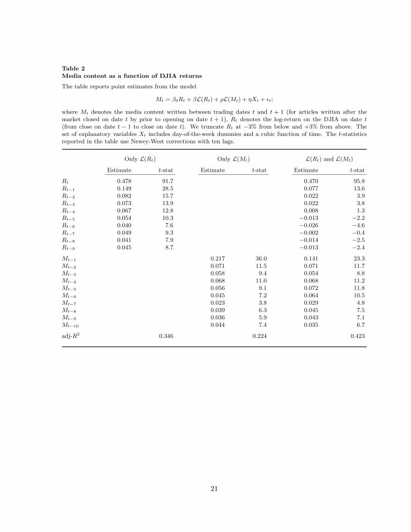
Table 2Media content as a function of DJIA returns

The table reports point estimates from the model

Mt = β0Rt + βL(Rt) + ρL(Mt) + ηXt + εt;

where Mt denotes the media content written between trading dates t and t + 1 (for articles written after themarket closed on date t by prior to opening on date t + 1), Rt denotes the log-return on the DJIA on date t(from close on date t − 1 to close on date t). We truncate Rt at −3% from below and +3% from above. Theset of explanatory variables Xt includes day-of-the-week dummies and a cubic function of time. The t-statisticsreported in the table use Newey-West corrections with ten lags.

Only L(Rt) Only L(Mt) L(Rt) and L(Mt)

Estimate t-stat Estimate t-stat Estimate t-stat

Rt 0.478 91.7 0.470 95.8Rt−1 0.149 28.5 0.077 13.6Rt−2 0.082 15.7 0.022 3.9Rt−3 0.073 13.9 0.022 3.8Rt−4 0.067 12.8 0.008 1.3Rt−5 0.054 10.3 −0.013 −2.2Rt−6 0.040 7.6 −0.026 −4.6Rt−7 0.049 9.3 −0.002 −0.4Rt−8 0.041 7.9 −0.014 −2.5Rt−9 0.045 8.7 −0.013 −2.4

Mt−1 0.217 36.0 0.141 23.3Mt−2 0.071 11.5 0.071 11.7Mt−3 0.058 9.4 0.054 8.8Mt−4 0.068 11.0 0.068 11.2Mt−5 0.056 9.1 0.072 11.8Mt−6 0.045 7.2 0.064 10.5Mt−7 0.023 3.8 0.029 4.8Mt−8 0.039 6.3 0.045 7.5Mt−9 0.036 5.9 0.043 7.1Mt−10 0.044 7.4 0.035 6.7

adj-R2 0.346 0.224 0.423

21

Table 3Media content as a non-linear function of last DJIA return

The table reports point estimates from the model

Mt = f(Rt;α, β) + ηXt + εt;

where Mt denotes the media content written between trading dates t and t + 1 (for articles written after themarket closed on date t by prior to opening on date t+ 1), Rt denotes the log-return on the DJIA (truncated at−3% from below and +3% from above). The set of explanatory variables Xt includes 10 lags of Rt and Mt, aswell as day-of-the-week dummies and a cubic function of time. The function f(Rt;α, β) is assumed to be of theform

f(Rt;α, β) =

4∑i=1

(αi + βiRt)1Rt∈Si (6)

where the sets Si are: S1 = (−3,−1), S2 = (−1, 0), S3 = (0, 1), and S4 = (1, 3). All statistics reported in thetable use Newey-West corrections with ten lags. The time period goes from January 3, 1905 through December31, 2005, for a total of 27,448 trading days.

A. Point estimates Intercepts Slopesαi t-stat βi t-stat

S1 = (−3,−1) −0.452 −6.1 0.203 8.6S2 = (−1, 0) 0.007 0.1 0.656 22.5S3 = (0, 1) 0.161 2.6 0.528 21.0S4 = (1, 3) 0.577 7.8 0.057 2.5

B. TestsF -stat p-value

α2 = α3 75.1 0.000β2 = β3 11.3 0.001β1 = β4 20.0 0.000

22

Table 4Media content as a function of multiple DJIA lagged returns

The table reports point estimates from the model

Mt = f1(Rt;α1, β1) + f2(Rt−1;α2, β2) + f3(Rt−2;α3, β3) + f4(Rt−3;α4, β4) + ηXt + εt;

where Mt denotes the media content written between trading dates t and t + 1 (for articles written after themarket closed on date t by prior to opening on date t+ 1), Rt denotes the log-return on the DJIA (truncated at−3% from below and +3% from above). The set of explanatory variables Xt includes day-of-the-week dummiesand a cubic function of time. The function fj(Rt;α, β) is assumed to be of the form

fj(Rt−j ;αj , βj) =

4∑i=1

(αji + βjiRt−i)1Rt−i∈Si (7)

where the sets Si are: S1 = (−3,−1), S2 = (−1, 0), S3 = (0, 1), and S4 = (1, 3). All statistics reported in thetable use Newey-West corrections with ten lags. The time period goes from January 3, 1905 through December31, 2005, for a total of 27,448 trading days.

A. Point estimates Intercepts Slopesαji t-stat βji t-stat

1. Return last trading day.S1 = (−3,−1) −0.469 −5.9 0.240 9.3S2 = (−1, 0) −0.002 0.0 0.699 22.5S3 = (0, 1) 0.154 2.3 0.516 19.4S4 = (1, 3) 0.573 7.4 0.027 1.1

2. Return two-days ago.S1 = (−3,−1) −0.114 −1.5 0.185 7.9S2 = (−1, 0) −0.051 −0.8 0.248 8.6S3 = (0, 1) −0.053 −0.8 0.109 4.0S4 = (1, 3) −0.010 −0.1 0.025 1.0

3. Return three-days ago.S1 = (−3,−1) −0.052 −0.7 0.113 4.7S2 = (−1, 0) 0.009 0.1 0.155 5.1S3 = (0, 1) −0.006 −0.1 0.047 1.7S4 = (1, 3) 0.092 1.2 −0.057 −2.2

4. Return four-days ago.S1 = (−3,−1) −0.010 −0.1 0.094 3.7S2 = (−1, 0) −0.003 −0.1 0.099 3.3S3 = (0, 1) 0.040 0.6 0.006 0.2S4 = (1, 3) 0.035 0.4 −0.008 −0.3

23

Table 4 continued.

B. TestsF -stat p-value

1. Return last trading day.α2 = α3 67.7 0.000β2 = β3 20.5 0.000β1 = β4 35.4 0.000

2. Return two-days ago.α2 = α3 0.1 0.903β2 = β3 12.1 0.001β1 = β4 21.7 0.000

3. Return three-days ago.α2 = α3 0.6 0.444β2 = β3 6.9 0.009β1 = β4 23.7 0.000

4. Return four-days ago.α2 = α3 4.9 0.027β2 = β3 5.4 0.020β1 = β4 8.0 0.005

24

Table 5Media content response for different authors

The table reports point estimates from the model

Mt = f(Rt;α, β) + ηXt + εt;

where Mt denotes the media content written between trading dates t and t + 1 (for articles written after themarket closed on date t by prior to opening on date t + 1), Rt denotes the log-return on a given stock index(truncated at −3% from below and +3% from above). The regression is run independently for each of the listedten authors of the column “Abreast-of-the-market,” published in the Wall Street Journal. The column labelledN presents the number of articles for each author. The set of explanatory variables Xt includes 5 lags of Rt andMt, as well as day-of-the-week dummies and a cubic function of time. The function f(Rt;α, β) is assumed to beof the form

f(Rt;α, β) =

4∑i=1

(αi + βiRt)1Rt∈Si (8)

where the sets Si are: S1 = (−3,−1), S2 = (−1, 0), S3 = (0, 1), and S4 = (1, 3). The time period is 1970–2005.All statistics reported in the table use Newey-West corrections with ten lags.

β1 β2 β3 β4

N Estimate t-stat Estimate t-stat Estimate t-stat Estimate t-stat

Hillery 2413 0.333 3.3 0.871 9.3 0.636 6.5 0.113 1.3Obrien 1215 0.533 3.5 1.169 5.1 1.069 5.2 0.218 1.5Talley 915 −0.025 −0.1 1.111 5.4 1.097 5.3 −0.258 −1.3Marcial 625 0.899 2.3 0.430 1.5 0.830 2.8 −0.169 −0.5Garcia 588 0.289 1.4 1.469 6.1 0.597 2.7 −0.112 −0.7Smith 302 −0.246 −0.6 1.124 3.7 0.945 3.0 −0.078 −0.3Wilson 251 0.037 0.1 0.988 2.9 0.656 2.4 0.397 1.3Browning 250 0.592 1.6 0.156 0.4 0.198 0.5 −0.066 −0.2Pettit 222 0.307 0.4 1.313 3.6 0.218 0.5 −0.587 −0.4Sease 157 0.624 1.8 0.735 1.6 −0.017 −0.0 0.648 0.8

25

Table 6Media content in different time periods

The table reports point estimates from the model

Mt = f(Rt;α, β) + ηXt + εt;

where Mt denotes the media content written between trading dates t and t + 1 (for articles written after themarket closed on date t by prior to opening on date t + 1), Rt denotes the log-return on a given stock index(truncated at −3% from below and +3% from above). The set of explanatory variables Xt includes 5 lags of Rt

and Mt, as well as day-of-the-week dummies and a cubic function of time. The function f(Rt;α, β) is assumedto be of the form

f(Rt;α, β) =

4∑i=1

(αi + βiRt)1Rt∈Si (9)

where the sets Si are: S1 = (−3,−1), S2 = (−1, 0), S3 = (0, 1), and S4 = (1, 3). Each column presents the pointestimates for different subsamples: 1905–1930, 1931–1955, 1956–1980, 1981–2005. All statistics reported in thetable use Newey-West corrections with ten lags.

A. Point estimates

1905–1930 1931–1955 1956–1980 1981–2005

Estimate t-stat Estimate t-stat Estimate t-stat Estimate t-stat

β1 0.241 5.7 0.255 7.3 0.286 4.2 0.236 3.9β2 0.459 8.2 0.652 13.0 0.770 14.7 0.794 11.8β3 0.375 8.4 0.497 11.8 0.602 12.6 0.604 9.2β4 0.024 0.6 0.067 2.1 0.094 1.5 0.116 2.2

α1 -0.094 -0.8 -0.311 -2.3 -0.716 -4.7 -0.484 -2.3α2 0.196 2.1 -0.050 -0.4 -0.219 -1.9 0.122 0.7α3 0.319 3.4 0.030 0.3 -0.039 -0.3 0.397 2.1α4 0.647 5.5 0.371 2.9 0.355 2.4 0.860 4.2

B. Tests

F -stat p-value F -stat p-value F -stat p-value F -stat p-value

α2 = α3 12.9 0.000 8.4 0.004 28.1 0.000 34.1 0.000β2 = β3 1.3 0.249 5.9 0.015 5.6 0.018 4.1 0.043β1 = β4 12.4 0.000 15.1 0.000 4.2 0.039 2.3 0.129

26

Table 7Media content as a non-linear function of other indexes

The table reports point estimates from the model

Mt = f(Rt;α, β) + ηXt + εt;

where Mt denotes the media content written between trading dates t and t + 1 (for articles written after themarket closed on date t by prior to opening on date t + 1), Rt denotes the log-return on a given stock index(truncated at −3% from below and +3% from above). The set of explanatory variables Xt includes 5 lags of Rt

and Mt, as well as day-of-the-week dummies and a cubic function of time. The function f(Rt;α, β) is assumedto be of the form

f(Rt;α, β) =

4∑i=1

(αi + βiRt)1Rt∈Si (10)

where the sets Si are: S1 = (−3,−1), S2 = (−1, 0), S3 = (0, 1), and S4 = (1, 3). Return information is fromKen French’s website. In the column labelled “VW index” we use his value-weighted index, whereas in the otherswe use the largest and smallest quintile portfolios in size. All statistics reported in the table use Newey-Westcorrections with ten lags. The time period goes from July 1st of 1963 through December 31st of 2005, for a totalof 12958 trading days.

A. Point estimates

VW index Large stocks Small stocks

Estimate t-stat Estimate t-stat Estimate t-stat

β1 0.209 4.3 0.281 5.9 0.140 2.5β2 0.826 18.6 0.815 18.1 0.874 17.2β3 0.682 16.3 0.661 15.5 0.702 15.8β4 0.005 0.1 0.055 1.3 0.036 0.6

α1 −0.580 −4.8 −0.352 −2.8 −0.692 −5.0α2 −0.028 −0.3 0.067 0.7 −0.077 −0.7α3 0.152 1.7 0.199 2.0 0.084 0.8α4 0.685 6.0 0.658 5.5 0.558 3.9

B. Tests

F -stat p-value F -stat p-value F -stat p-value

α2 = α3 41.2 0.000 20.9 0.000 29.8 0.000β2 = β3 5.7 0.017 6.3 0.012 6.6 0.010β1 = β4 9.2 0.002 12.4 0.000 1.5 0.216

27

Table 8Media content and DJIA returns along the business cycle

The table reports point estimates from the model

Mt = DtfR(Rt;α, β) + (1−Dt)fE(Rt;α, β) + ηXt + εt;

where Mt denotes the media content written between trading dates t and t + 1 (for articles written after themarket closed on date t by prior to opening on date t + 1), Dt is a dummy variable that equals 1 if date t is ina recession (using NBER definitions), Rt denotes the log-return on the DJIA (truncated at −3% from below and+3% from above). The set of explanatory variables Xt includes 10 lags of Rt and Mt, as well as day-of-the-weekdummies and a cubic function of time. The function fk(Rt;α, β) is assumed to be of the form

fk(Rt;α, β) =

4∑i=1

(αki + βkiRt)1Rt∈Si (11)

where the sets Si are: S1 = (−3,−1), S2 = (−1, 0), S3 = (0, 1), and S4 = (1, 3), and k = R,E. All statisticsreported in the table use Newey-West corrections with ten lags. The time period goes from January 3, 1905through December 31, 2005, for a total of 27,448 trading days.

A. Point estimates

Expansions Recessions

Estimate t-stat Estimate t-stat

βk1 0.236 7.0 0.242 7.4βk2 0.694 20.6 0.560 9.7βk3 0.559 19.2 0.404 7.7βk4 0.050 1.7 0.065 1.8

αk1 −0.503 −5.6 −0.206 −1.4αk2 −0.021 −0.3 0.092 0.7αk3 0.139 1.9 0.215 1.7αk4 0.585 6.7 0.529 3.6

B. Tests

F -stat p-value F -stat p-value

αk2 = αk3 60.8 0.000 11.2 0.001βk2 = βk3 9.6 0.002 4.0 0.046βk2 = βk3 16.7 0.000 13.0 0.000

28

Table 9Media content as a function of last day’s DJIA return, eight intervals

The table reports point estimates from the model

Mt = f(Rt;α, β) + ηXt + εt;

where Mt denotes the media content written between trading dates t and t + 1 (for articles written after themarket closed on date t by prior to opening on date t+ 1), Rt denotes the log-return on the DJIA (truncated at−3% from below and +3% from above). The set of explanatory variables Xt includes 10 lags of Rt and Mt, aswell as day-of-the-week dummies and a cubic function of time. The function f(Rt;α, β) is assumed to be of theform

f(Rt;α, β) =

8∑i=1

(αi + βiRt)1Rt∈Si (12)

where the sets Si are: S1 = (−3,−2), S2 = (−2,−1), S3 = (−1,−0.5), S4 = (−0.5, 0), S5 = (0, 0.5), S6 = (0.5, 1),S7 = (1, 2) and S8 = (2, 3). All statistics reported in the table use Newey-West corrections with ten lags. Thetime period goes from January 3, 1905 through December 31, 2005, for a total of 27,448 trading days.

A. Point estimates Intercepts Slopesαi t-stat βi t-stat

S1 = (−3,−2) −0.263 −1.2 0.266 3.3S2 = (−2,−1) −0.316 −3.0 0.309 4.9S3 = (−1,−0.5) −0.142 −1.5 0.455 4.7S4 = (−0.5, 0) 0.021 0.3 0.711 11.3S5 = (0, 0.5) 0.102 1.6 0.806 13.3S6 = (0.5, 1) 0.280 3.3 0.346 4.4S7 = (1, 2) 0.543 5.4 0.079 1.4S8 = (2, 3) 0.996 4.8 −0.100 −1.3

B. TestsF -stat p-value

α4 = α5 11.6 0.001β4 = β5 1.2 0.271β3 = β6 0.7 0.387β2 = β7 7.5 0.006β1 = β8 11.3 0.001

29

−3 −2 −1 0 1 2 3

−1.

0−

0.5

0.0

0.5

1.0

Media content and stock returns

Previous trading day DJIA returns

Pos

itive

− N

egat

ive

wor

ds (

%)

Figure 1The graph presents three estimates of the relationship between media content and lagged DJIA returns. Thecrosses denote the average unconditional media content for intervals of 2 basis points on the range of returns(−3, 3). The solid smooth black line presents a spline estimator, with 95% confidence intervals as dashed lines.The straight lines are OLS estimates using piece-wise linear functions over the intervals (−3,−1), (−1, 0), (0, 1)and (1, 3). The rug in the x-axis presents the density of the right-hand side variable.

30

−3 −2 −1 0 1 2 3

−1.

0−

0.5

0.0

0.5

1.0

Media content and stock returns previous four trading days

Previous trading day DJIA returns

Pos

itive

− N

egat

ive

wor

ds (

%)

Figure 2The graph presents four estimates. They measure the relationship between media content and: (1) one-day laggedDJIA returns (solid line), (2) two-day lagged DJIA returns (dashed line), (3) three-day lagged DJIA returns, and(4) four-day lagged DJIA returns. The lines in the graphs represent the OLS estimates using piece-wise linearfunctions over the intervals (−3,−1), (−1, 0), (0, 1) and (1, 3) of the specification in Table 4. The rug in the x-axispresents the density of the right-hand side variable.

31