THE KINEMATICS OF BREAKING

WAVES IN THE SURF ZONE.

Alfred James 01 sen

NAVAL POSTGRADUATE SCHOOL

Monterey, California

THESISTHE KINEMATICS OF BREAKING WAVES

IN THE SURF ZONE

by

Alfred James 01 sen

September 1977

Thesis Advisor: Edward B. Thornton

Approved for public release; distribution unlimited.

T181457

SECURITY CL ASSIFICATION OF THIS PAGE (Whan Data Knfrod,

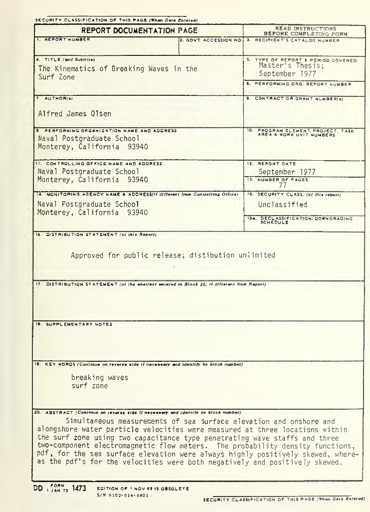
REPORT DOCUMENTATION PAGE READ INSTRUCTIONSBEFORE COMPLETING FORM

T. REPORT NUMBER 2. GOVT ACCESSION NO 3. RECIPIENT'S CATALOG NUMBER

4. TITLE (and Submit)

The Kinematics of Breaking Waves in the

Surf Zone

3. TYPE OF REPORT * PERIOO COVEREDMaster's Thesis;September 1977

6. PERFORMING ORG. REPORT NUMBER

7. AuTHORr*; 8. CONTRACT OR GRANT NUMBERf*;

Alfred James 01 sen

9. PERFORMING ORGANIZATION NAME AND AOORESS

Naval Postgraduate SchoolMonterey, California 93940

10. PROGRAM ELEMENT. PROJECT TASKAREA b WORK UNIT NUMBERS

II. CONTROLLING OFFICE NAME AND ADORESS

Naval Postgraduate SchoolMonterey, California 93940

12. REPORT DATE

September 197713. NUMBER OF PAGES

77TT MONITORING AGENCY NAME a AOORESSf// dlllarant from Controlling Olllca)

Naval Postgraduate SchoolMonterey, California 93940

15. SECURITY CLASS, (ol thta riporl)

Unclassified

IS*. DECLASSIFICATION/ DOWNGRADINGSCHEDULE

16. DISTRIBUTION STATEMENT (ol ihl* Raport)

Approved for public release; distibution unlimited

17. DISTRIBUTION STATEMENT (ol tha abatraet antarad In Block 20, II dlttarant from Raport)

18. SUPPLEMENTARY NOTES

19. KEY WORDS (Continue on ravaraa alda It nacaaaary and Idantity by block numbar)

breaking wavessurf zone

20. ABSTRACT (Contlnua on ravaraa alda II nacaaaary and Idantity by block numbar)

Simultaneous measurements of sea surface elevation and onshore andalongshore water particle velocities were measured at three locations withinthe surf zone using two capacitance type penetrating wave staffs and threetwo-component electromagnetic flow meters. The probability density functions,pdf , for the sea surface elevation were always highly positively skewed, where-as the pdf s for the velocities were both negatively and positively skewed.

do ,;"STt. 1473 EDITION OF I NOV 88 IS OBSOLETES/N 0102-014- 6601

I

SECURITY CLASSIFICATION OF THIS PAOe (Whan Data Mntarad)

Approved for public release; distribution unlimited

The Kinematics of Breaking Waves

in the Surf Zone

by

Alfred James 01 sen

Lieutenant, United States Navy

B.S., United States Naval Academy, 1972

Submitted in partial fulfillment of therequirements for the degree of

MASTER OF SCIENCE IN OCEANOGRAPHY

from the

NAVAL POSTGRADUATE SCHOOLSeptember 1977

ABSTRACT

Simultaneous measurements of sea surface elevation and onshore and

alongshore water particle velocities were measured at three locations

within the surf zone using two capacitance type pentrating wave staffs

and three two-component electromagnetic flow meters. The probability

density functions, pdf, for the sea surface elevation were always highly

positively skewed, whereas the pdf's for the velocities were both nega-

tively and positively skewed. Mean values of the onshore and alongshore

components of flow reflected the influence of a rip current frequently

observed just south of the instrument locations. Strong harmonics in

the spectra of sea surface fluctuations and particle velocities infer

nonlinear conditions. Coherence values between waves and onshore flow

were high, ranging above 0.9. The coherence between waves and onshore

flow was used to separate the turbulence and wave-induced velocity

components. Over the range of collapsing to spilling breakers a rea-

sonable value for the ratio of turbulent to wave-induced velocity was

determined to be approximately 0.75. Saturation regions were found in

the wave and velocity energy-density spectra at higher frequencies as

evidenced by -5 and -3 slopes, respectively.

TABLE OF CONTENTS

I. INTRODUCTION 9

A. HISTORICAL PERSPECTIVE 9

B. OBJECTIVES - 10

II. MEASUREMENTS 12

A. EXPERIMENT - 12

B. INSTRUMENTATION 14

III. ANALYSIS OF DATA 21

IV. RESULTS 25

A. QUALITATIVE DESCRIPTION 25

B. MEAN VALUES 25

C. PROBABILITY DENSITY FUNCTIONS 27

1. Gaussian and Gram-Charl ier Frequency Distributions 27

2. Skewness and Kurtosis 28

D. SPECTRAL ANALYSIS 31

1. Sea Surface Elevation and water particle velocity 31

2. Onshore flow and alongshore flow 34

E. TURBULENT VELOCITY INTENSITY AND WAVE-INDUCED VELOCITYINTENSITY 36

F. SATURATION REGION IN THE SPECTRUM OF BREAKING WAVES 42

V. CONCLUSIONS 48

APPENDIX A - BEACH PROFILES 50

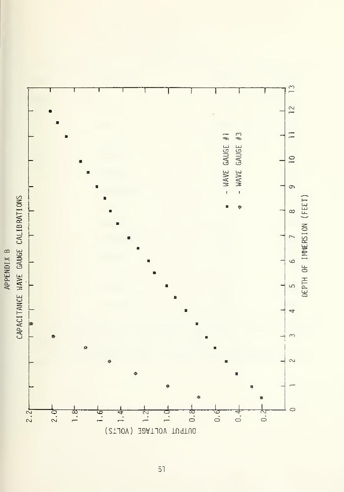
APPENDIX B - CAPACITANCE WAVE GAUGE CALIBRATIONS 51

APPENDIX C - CALIBRATION FACTORS 52

APPENDIX D - PROBABILITY DENSITY FUNCTIONS 53

APPENDIX E - POWER, COHERENCE AND PHASE SPECTRA 6 7

5

LIST OF TABLES

I. Beach and Wave Characteristics 15

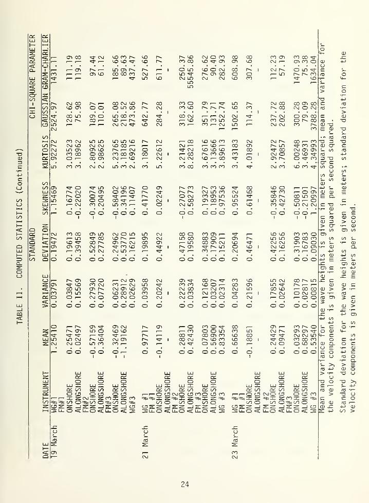
II. Computed Statistics 23

III. Ratio of Coherences of short crested waves tolong crested waves 41

LIST OF FIGURES

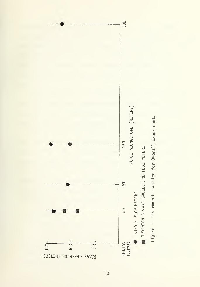
1. Instrument Location for Overall Experiment 13

2. Typical Beach Profile and Instrument Location

at Torrey Pines Beach on 19 March 1 6

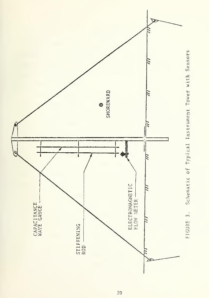
3. Schematic of Typical Instrument Tower with Sensors 20

4. Typical Analog Record of Waves and Onshore Velocitiesfrom Torrey Pines Beach 26

5. Frequency Distribution of the Sea Surface Elevationat Wave Gauge #1 on 23 March 1977 29

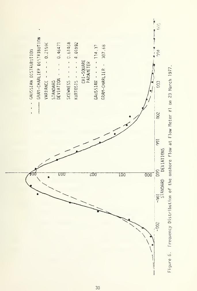
6. Frequency Distribution of the onshore flow at FlowMeter #1 on 23 March 1977 30

7. Power, Coherence and Phase Spectra for the onshore flowof Flow Meter #1 and Wave Gauge #1 on 23 March 32

8. Power, Coherence and Phase Spectra for the onshore andalongshore components of flow at Flow Meter #3 on 23 March 35

9. Ratio of turbulent to wave-induced velocity intensities 38

10. Sea Surface Elevation Spectra at Wave Gauge #1 44

11. Sea Surface Elevation Spectra at Wave Gauge #3 45

12. Onshore Water Particle Velocity Spectra at Flow Meter #1 46

13. Onshore Water Particle Velocity Spectra at Flow Meter #3 47

ACKNOWLEDGEMENTS

I would like to express my deep appreciation to Dr. Edward B.

Thornton for his understanding, knowledge and assistance without

which this project would not even have started, much less reach fruition

I would also like to thank my wife, Dana, for her patience and typing.

Of particular assistance was the Computer Center "night crew."

I. INTRODUCTION

A. HISTORICAL PERSPECTIVE

The surf zone is an area bounded on the seaward side by the point

where waves first begin to break, and on the landward side by the point

of maximum run-up on the beach slope. Although beach profiles and waves

within the surf zone have been studied by many, the kinematics of wave

forms and water particle velocities in the zone have remained something

of a mystery.

The problems encountered have been practical as well as theoretical.

Wave theories developed for deep water waves do not correctly characterize

the motion which occurs as the waves break. Direct measurements of break-

ing waves appear to be the most viable means of approaching the problem.

However, this has been hampered by the surf zone's hostile environment,

which is difficult to reproduce in the laboratory, and by inadequate

instrument design. Improvements in the latter area has resulted in sturdy,

sensitive, but expensive measuring devices which have rapid response times.

The earliest study of significant importance was conducted by

Iversen (1953) in which he used photographic techniques to obtain a

Lagrangian description of water particle motion under breaking waves.

The laboratory channel limited the wave type to plunging and surging

breakers.

Inman (1956) was one of the first to make sophisticated field

measurements, measuring the drag force on a canti levered sphere to infer

water particle motion. Miller and Zeigler (1964) measured in situ

particle motions using acoustic and electromagnetic current meters,

then compared their findings with higher order wave theory and found

some qualitative agreement. Walker (1969) made similar measurements

using propeller type flow meters. Meadows (1976) used ducted impeller

flow meters at equally spaced vertical positions in order to measure

longshore components of flow. Huntley (1976) utilized a single two-

component electromagnetic flow meter in an effort to obtain a value

of the friction coefficient. Bowen and Huntley (1974) made measure-

ments of the nearshore velocity fields using as many as three two-

component electromagnetic flow meters. Fuhrbdter and Busching (1974)

measured simultaneous orbital velocities and water levels using a two-

component current meter and two pressure type wave meters. Thornton

(1969), Steer (1972), Thornton and Richardson (1973), Bub (1974) and

Galvin (1975) used pressure meters, capacitace wave gauges and electro-

magnetic current meters to compute particle velocities and surface profiles

within the surf zone. The work presented herein is an extension of these

latter studies.

B. OBJECTIVE

The objective of this research is to study the kinematics of water

particles within breaking waves and within the surf zone. In particular,

the experiment was performed on a flat beach in order to measure the

characteristics of spilling breakers. Simultaneous measurements were

made of the instaneous sea surface elevation and two orthogonal water

particle velocities, onshore and alongshore, at three fixed locations

in the surf zone. Estimates of the probability density functions and

10

power spectra of the wave heights and particle velocities are made. The

suitability of using linear wave theory as a spectral transfer function

in determining velocity spectral components from the power spectrum of

the waves is measured. Computed velocity spectra are compared with

actually measured velocity spectra. Coherence between waves and onshore

flow is used to separate the turbulence and wave-induced velocity com-

ponents in order to determine the ratio of turbulent to wave-induced

velocity. Spectral estimates are analyzed to ascertain the slope of

the saturation region at higher frequencies.

11

II. MEASUREMENTS

A. EXPERIMENT

The experimental site is just north of La Jolla, California. Data

presented in this study was taken as part of a larger scale experiment

conducted from 15 February to 30 March 1977 in the Southern California

bight area. The over-all purpose of the experiment was to test and

evaluate the instrumentation package which was selected for use aboard

SEASAT. The apparatus, which will measure waves, winds, and sea surface

temperature, was being flown on board NASA airplanes. A major ground

truth program was concurrently being conducted at Torrey Pines Beach.

Measurements of waves, currents, and sediment transport at Torrey

Pines Beach were made using the following equipment. A five element

linear array of pressure sensors was positioned offshore along the ten

meter contour to measure wave energy and direction. Located in the surf

zone inshore of the array were three support towers in a line perpendi-

cular to the beach. A surface piercing capacitance wave gauge and a two-

component electromagnetic flow meter were mounted on each tower. A

nephelometer was installed on the middle support tower. To the north

of the three towers was an array of four flow meters which was used to

delineate the area! and temporal variation in alongshore currents.

Figure 1 shows instrument locations. Resistance-wire run-up meters were

installed in the swash zone at four locations. All instrumentation

was battery operated.

The offshore pressure sensor outputs were telemetered directly to

the shore processes lab at Scripps Institute of Oceanography, which is

12

oen

<*un

<b- 4U">

(SH1L3W) BUOHSJJO 39NVH

ooq:UJf- .— -«->s E

UJcc £

O)n: Q.oo XCO UJo 2:

LO .

—

^—1 on ,

—

<cUJ

<T3

5-UJ 1— 0)

UJ

_lU_

>OS-

<+-

CO•t—4->o 03

CT>

<J->

00UJ

OO_l

cc <=C 4->

UJ Ch- O)UJ LU cr

21 >< 3O 3: 3 +->

LO to_J (/) cu_

2:1—

1

on O 1

— 1— r—<=c -ziM r>s

<DO S-O1—

=3

2: s: • u_

=C»—

4

>-O T^25 «=c>—

1

13

located one mile to the south. All data from the other instruments

were cabled to one of two transmitting terminals on the beach where it was

then telemetered to the shore processes lab and recorded. All the equip-

ment except the nephelometer were in position prior to high tide on 9

March. The nepholometer was installed on 14 and 15 March. Data was

accumulated during high tide on 9, 10, 11, 16, 17, 18, 19, 21 and 23

March.

Several other smaller scale experiments were conducted at the same

time. At an elevation of approximately 300 feet on a cliff overlooking

Torrey Pines Beach a radar installation was established. The radar

images of waves were then photographed and analyzed.

Sediment transport experiments were conducted on 11, 21, and 23

March. Bed load transport was measured using the methods described by

Inman and Komar (1970) to trace the movement of fluorescent dyed sand.

Suspended sediments were measured in situ by swimmers using a mechanical

water sampling devide. These samples were taken along with nepholometer

readings in order to compare methods. During these sediment transport

investigations, Lagrangian floats made from wine bottles weighted by

sand were used to determine average long-shore current speeds.

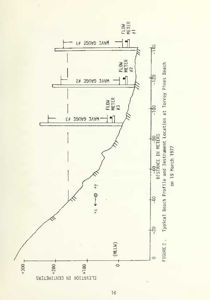
B. INSTRUMENTATION.

The manner in which waves break depends wery much on the character-

istics of the beach and near shore bottom slope. (Table I) Spilling breakers

occurred most frequently at the Torrey Pines Beach site. Figure 2 shows

a typical beach profile and the location of the instruments which provided

the data for this paper.

14

TABLE I. BEACH AND WAVE CHARACTERISTICS

LOCATION

DATE

BEACH SLOPE

SAND TYPE

SAND MEDIAN GRAIN SIZE

BREAKER TYPE

WAVE PERIOD

WAVE HEIGHT

TORREY PINES BEACH

9-23 MARCH 1977

FIGURE 2 and APPENDIX A

QUARTZ

1.2 MILLIMETERS

SPILLING

11.9 to 15.9 SECONDS

UP TO 1.5 METERS

15

3 LUO h-I LU i

—

u_ 2: =*t

+ +

SH313WI1N30 MI N0UVA313

16

1 . Wave Gauge

The wave gauges were of the capacitance type fashioned from

3/8 inch outside diameter stainless steel rod. The rod was tightly

covered with 1/16 inch wall thickness polypropylene tubing. This li-

near, highly sensitive instrument has proven to be sufficiently sturdy

to withstand the rigors of the unfriendly surf zone. The gauges operate

on the principle that a change in the plate dimension of the capacitor

changes its capacitance and consequently the circuitry output voltage.

In these gauges, the insulated steel rod and sea water act as the plates

and the insulation functions as the dielectric. As the water level fluc-

tuated, the capacitance changed. Fluctuations were sensed by a transis-

torized circuit powered from the beach. The circuit was designed by

McGoldrick (1969). The electronics packaged was housed in a watertight

brass case which was mounted on the tower. This allowed the connecting

leads to be relatively short, hence minimizing wire-to-wire capacitance.

All gauges were statically calibrated in the laboratory prior to the ex-

periment. Accuracy was estimated to be -.005m. The calibration plots

are shown in Appendix B.

17

2. Flow Meter

The flow meters were Marsh-McBirney model 511 electromagnetic

water current meters. Operation of the meter is based on Faraday's prin-

ciple of electromagnetic induction. The meter measures water particle

velocity in two orthogonal directions through a range of zero to three

m/sec with a maximum output error of two percent of full scale reading.

The sensor has a variable time constant, a setting of 0.2 sec. was used.

The flow meters were dynamically calibrated using the method of

Thornton and Krapohl (1974). This procedure involves utilizing an os-

cillating platform driven by a variable speed motor geared to an eccen-

tric throw arm. This technique was employed in order to determine the

meter's characteristics. Measurement accuracy was determined to be

±.005 m/sec. The only difficulty encountered in their utilization oc-

curred when Flow Meter #1 was buried on 19 March due to the heavy sedi-

ment transport.

The measuring instruments were attached to a 3.6m high tower con-

structed of steel pipe with an outside diameter of 6. 3cm. A 0.5m diameter

base plate was placed about 0.6m from the bottom of the tower. This

configuration allowed the tower to be sunk approximately 0.7m into the

sand. The towers were also supported by steel guy wires fastened to

blade anchors driven into the sand. Thus, tower movement and vibration

were negl igible.

The towers were placed on a line perpendicular to the shore at

specified distances, and were erected during low tide when the beach

was more accessible. As indicated earlier, measurements were taken at

18

high tide. Instruments were arranged so as to be in the same vertical

plane. A carpenter's level was used to establish axis alignment with an

estimated error of -2 degrees. A typical tower and instrument arrangement

is shown in Figure 3.

19

k.

oen

C<u

GO

oH»J

C

E

>-.

C

urH

O

O•r-(

+->

e

u00

ft!

o

20

III. ANALYSIS OF DATA

The data were digitized at a rate of four samples per second,

corresponding to a sample interval of 0.25 seconds. This resulted in a

Nyquist frequence of 2.0 He. The sampling rate was considered suffi-

ciently high enough to avoid aliasing of energy into the portion of the

spectra which was of interest.

Continuous time series records of all measurements were taken for

roughly 2-1/2 hours each day. Record lengths of 24 minutes from each

data set were subjected to analysis. Criteria which determined record

lengths included economy of computer usage and resolution over the fre-

quency range of interest.

A maximum lag time was chosen as 5% of the record length. This re-

sulted in a spectral band width resolution of 0.007 He and each spectral

estimate having 40 degrees of freedom. The ninety percent confidence

limits for 40 degrees of freedom using a chi-square distribution are found

to be between 0.72 and 1.51 of the measured power spectral estimates.

A mean value was computed for all data sets and the data was linearly

detrended to remove tidal effects. Variance, standard deviation and

average period were calculated. The average period was determined by

calculating the time between zero upcrossings. The calculated average

periods are lower than the visually observed periods due to a number of

perturbations, such as noise and capillary waves, increasing the zero

upcrossing occurrences. A probability density function for each data set

was calculated and plotted. Comparisons were made with Gaussian and Gram-

Charlier distributions using the chi-square goodness-of-fit test. Variance,

21

standard deviation, skewness and kurtosis of the distributions were

computed and are summarized in Table II.

For each data set an auto-covariance function was determined and then

smoothed with a Parzen window. Applying a Fourier transform to the smoothed

auto-covariance function resulted in the power spectrum. An examination of

the power spectrum shows the regions of greatest potential or kinetic

energies and their respective frequencies.

Cross-spectra were computed by calculating a cross-covariance between

data sets, smoothing it with a Parzen window and applying a Fourier trans-

form. Coherence and phase were then determined from the cross-spectrum.

A coherence and phase versus frequency plot will indicate the regions

and degree of linear relationship and phase between two data sets.

22

Od QL

o

ooC_)

OOI—

I

I—<cI—oo

Q

oC_5

UJ_lCO

oo

OOoC£XD

OOOO

oo

Q OCC •—

I

=C I—Q =£z: >—

<

<c >UJ

OO Q

c_>

X)cr:

00

<

r^» l*>. r^ CO CNJ r^ ud r^ O uo CO r-~ ud CO OO CNJ O 1

—

CNJ CO UD r>1— uo ud CTl CO 10 '

—

i^> UD UD CDO ud OO r-^ '

—

O r— OO <3- m OO CTl

r^ CNJ IT) CO , •^f uo LT) , CNJ ,— 00 , r^. ,— 00 r^. 00 00 1

r^ CO CNJ r-^ UD CO r

—

r^ O OO in CNJ CNJ UD CNJ 00 UD 1

—

OO 1

—

"S3- LO UDCNJ

*d- OOCNJ

O

10 LO LO «3" ud en CNJ CNJ O ^_ UD CO «* m UD CO CO 00 O en _ ^rUD '

—

r^ O r^- UD UD r-^ UD CO ^r uo CO UO Cn 00 CO '

—

<— UD <—

O OO »3- CNJ O CD UD UD , 00 <=j- 00 >^- •3- OO «^r CO CO , , U3ro 1

—

O ^r CO CO 1

—

1— *d- cn 1

—

UO CNJ CNJ CNJ CNJ ro c UD 1

—

00 CMUD 1 1 r>« ' O

UO" CNJ "~

' UOuo

1 CNJ 1 r— en

cn OO . . CNJ ud «=3- uo cn O "=3- ** CNJ OO UD uo r^ UD CO UD p^ CTl r^(— cn CO r^ CNJ CO ro ^r cn OO <a- UD r^ 1

— O r— r— ^~ ^— UD UDCO CO r— CNJ 1

—

UD CO ud 00 OO ud r-«. CO uo r— CNJ r

—

Cn CTl CNJ CNJ•"» O 1— «a- r^ !-- CO 1 CTl CTl LT) "vT «3- r-» <^r 1 CNJ UD UO CO «3" 1^ ^rLO O UD CNJ UD O "" O O UO ^f- r- «5f m 1 CO CT» OO 1

— r^. ""

CNJ CO CO

o o

CO CO CO CO uo 00 CO 00 00 CNJ CO UD CO <^- CNJ CNJ

o o o o o o o o o o o o o o

3-

COCOCO

11879 09757

UD

COCOCNJ

CNJ

COCO 04116 58692

1 1 1

UJen

UJ

OUJ

oi r ujx uj zncc m cc 00 cz 00OC3 OO O C3 00-r-ZZCMXZOOIZ^fe% % l/l O =* W O * C/) Oozzjsz-jzzjo3u_o<a:u_o«=Cu_o><2

r^ CNJ 1

—

CNJ 1

—

en enUD CO ^~ UO en r— UDCNJ «sf p»» CO UD ^~ COUD UD CNJ CNJ 1

—

1— 1

CNJ «* CNJ CNJ 1

—

l— 1—

1

O

UJ

O

UJon

O1 1

UJ

UJ 3: UJ zc UJ acCZ 00 or 00 or: 00

CDr— 1

—

X ^ CNJ :n ^ 00 :r z: 00^ I* OO =*fc 00 =tte 00 O =»=O 2 s _1 s z _l SI ^ _1 O2 tLO< u_ <: u_ O < 2

OO CO «^-

r— UO cn r>~ ; ,

—

en CO UD CO r^ «vT -3- ,

—

UO r^ ro ,

—

,

—

,

—

CNJ UDCO CO UD r^ cn t— en r— r— ^~ UD 1

—

en UD uo uo 00 CNJ CO CNJ 00r^ UD CO CO CO uo CO CO UD r— CO en uo r-% <^- CNJ «a- *a- cn UO uor— 00 I

s- <3- r— uo CO 1 CNJ CO 1

—

CO CNJ ^1- uo 1 "5t co CNJ CNJ UO <d- CO uoCNJ 1

— '^~1— '— r— CO 1

— O

—

CNJ UD CNJ CNJ <— O — CNJ

O O1

O1

O O1

•— O1 1

O O1

- O O O O1

UO UO r-^ O OO CO O uo UO CNJ UO CO O <3" -Sj- cn cm UD CO *cr

cn CO ^~ UD CNJ -* r^ CNJ CNJ r— cn CO Bf CO r»» r— CNJ cn O uo UDCNJ ^r cn CNJ r-. UD r^ =a- UD CNJ en CNJ «* «* O <ct- 1— CO ^f UD 1

—

1

—

UD r— 1

—

CO CO cn 1 uo cn 1

—

CO en ro O 11

—

CO UD r™~ CO 1^. *tCNJ «^- CNJ CO •"" •=3" •— CNJ *d- CNJ «3-

1— uo CNJ CNJ uo CNJ <3" r— ,^- CNJ 1

—O O O O O O O O O O O

UO en co CO CO r~^ cn CNJ m ud CO CO CO >— ^1- ud r>» ud cn CO UD UDCO CO CO «* UO CO 1^. r^» cn CO CO ^~ cm r«. 1— UD MXJOuo UD CO CO 00 O cn •vl- O UD ud en CO .

—

UD r^ cn cn uo <3" CNJ O«d- r— «3" CO 1— cn co 1 UD <=r "vr CO CO co «d" 1 <i- CO UD UD CO CNJ <3" CNJO CNJ O r— O 1— O O CNJ O r- O CNJ O 00 r— CNJ O O

000

CNJ

COUDCNJCO

94626 49211 34363 70356 11006 22176

"—1 1

UJ UJcn

UJ

uITS

C£L OO Oi OO CH OOr^i— OOCNJOC3COOC3CO

OOO OOO OO ooszjzzjsz jo3u_o<=cu_o<=i:u_o<:s

UD CO

23

qc

QC<Q_

QC

OcrCO

i

CD

£Z

+->

cooCOo

OOI—

I

oo

Q

OO

OQC

Q

CO

CO

qc

qc

ZZ

O

COCOZD<cOCOI—

I

COoi—QC=>i*c

cooo

oI—

I

I—

I—CO

CO^1-

P-.CTi

CM

(XI

CM1^CMCM

LO

CTi

CO

LO

CM

cn

o

<3"

CM

CTi CO

r— CTi

*Zt CM•S3- r-

co co r-^co co -=3-

coco

r»- coco CO

cm o coCO <=f CTi

COCTi

COCO

CO CTi COCO *C\J i— CTi CO O

CM COCO CTi

f-» r—CTi CO

r^ i

—

O O

co CTi r-».

CO CO coi— *3"

C0 CM COO CO CO

CMLO co

COCM

O LOLO <vj-

CM LOLOLO

CO OCO CO

CO O CMr-- en coCM CM

CT> i— «^fr». r^ r>-

co l**o oco co

COCO CO

cm r^i— CO

CM COr--. CO

CO cocm r^

co CMCM COLO CTiCO COO i—

CTi OCO >—

LO LOCM CMCTi COO COCO CT>

CO CO COco i— r^»CM CM <=T

LO LO COCO CO r—r^ i— cmCO CO CTiCM i— CO

CM

cocoCM

O COCO CM•— CvJ

CO CMr— COCO i

—

r— COCM r—^ CM•— COCM CM

i— r— CMLO CO LOCO i— CM

CO CO COr— CO r—CO CO COr^ co entO r— CO

CMOLO

COCO

CO<3-

COCO CVJ CM LOCOCM CO LO CO CO CO CO CO CO

CMCTi

CO

o

l->» CMCO OCM CM

cm r-^r»«. lo<a- COCM O

<s- or^ cmr»- oCO CMi— CM

"vT LOr^ cnO ^rO OCO CM

cm co r^ocno"^i- 1— <^rco «^J- —LO CO i

—

O CTi

r^ cmi— CM I

«3- o

r^ co

O CMr*. coCM LO

rvco coCM LO COCO CTi LOcn co r--r— r— CTi

CMLOLOCTi

i— OO OO OOO O O OOO

COCO<=T

co

o

CO o<3- COco r-.LO CMCO ^T

CO COi LOco «d-CT> CTii— CO

CTi LO«3" COco r^cm r-»LO CM

CM O LOCONi

—

CT> r^ CM^j" CO COCM CO i

—

COCTi

COCTi

CMCMCTi

CO oLO 00f— LOr-^ <Ti53- t—

CO CTi i

—

CO O i—CO CTi CM•^- r->. loCO i— i

—

<3-

CTi

COoCM

co l

CO COLO LOCM CMCM CO^J" r—

O O O O OOO O O OOO

•

—

r-N cn o o r— CM CTi CO CM cn «=r CO r^ <vi- CO COCTi <3- CO CO CM CO r— CM LO ^J" CO CO COOr- CO CTir*» CO LO CTi r-. CM CTi CO CTi CM CM CO i— CM CO CM LOCO CO LO r^ r^ CO CO CM CO O 1 CM CO CM CO CM <tf- ^—o o •— CM O O CM O O CM CM O r- O O o CM

LO CMLO <^"

CO COI^s. CMr— O

OO OO OOO o O O OOO

o .—r*. cn=3- ^rLO CMCM O

CT. «*LO Or- ^fr-- coLO CO

CTi CMCO CO^- r—CM CTi

CO i

—

r~- CTi

r~- i

—

i^- -=3-

CTi i—

i— o o o o o .— Ol

1

—

o CO o «d" CO ,

—

CTi i

—

1

—

CO o o LO CO LO CM r-«»

co "vT CO CT CO CO CO «3- <=i-

CO CM r^ CO CO CO CO 1«3- CTi

CM «3- o LO CO CO •— CM Oo o o o o o o

1

O O

QCO O!_1

cco QCoLlJ

QCO QCOQC CO QC CO QC COO O O O O O

<— >— nr zwizcniz co^fe^JfcCO 0=tteCOO=teCOO =«te

02:2: JZZJZZJO3U.O cCLL,Od:Li_0<C 3

QC CO QC OO QC CO1— 1—OOCMOOCOOO CO=tt= ;«=3z s ::*fea: ^=«:rc z: =«=

CO O CO O CO osli_o=3:ll.oc3:li_0'=c s

us-

Ocnt1^. r^ co

CO CTi COCM O CM

O CTio r^CO

CO 1—^f COCM CTiO COO "Sf

o4-

QJ

Ucrot—

S_

>

to

03 •

0> T3E <D

S_fOZ3CTco

cm co co co «sr

1— oCO LOO r—LO CM

OO O O 1—

CO COO COcn r^r— coCO 1—

OO OOO

co r^ lor^ .— 1

—

-— CO COO CM O.— 00

OO OOO

rorv oCT> CT> «3"

CM CM LOCO 00 COO CO LO

CTi

CM

OOO

LU UJ LUQC QC QCOOO

UJ 3Z LU DZ LU ZZQC CO QC CO QC CO

1— 1—O O CMO O O O CO^tfc^fczc^^fezz zrozz =«=

OO O OO 0=**=00 Oc5sz-isz jzzjc33llo< llo <:li_o<: s

os-03

COCM

"OOJs-n33 T3CT Cco O

Uco OJS_ co<D4-> i-O) O)E D_

c -or- <V

S-C (13

<D 3> crp- tocn

coco S_r- 0)

10 o;

DC •!- 4->

r- •- OJ O)CD J= EJZ C

O)O) >> -I-

(O cn

CO<1J -r-

JZ4-J CO

+->

QJ

COo_

oo

s- >>(O 4->

> -I-

ofo oc: 1

—

(T3 O)>

cfO O)CD JZ

24

IV. RESULTS

A. QUALITATIVE DESCRIPTION

Observation of various breaker types which occur on different beaches

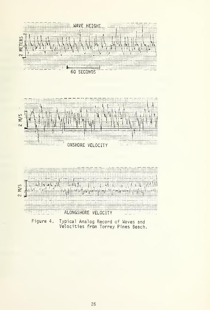
has resulted in a number of similarities being noted. A typical analog

record of waves and onshore velocities obtained at Torrey Pines Beach is

shown in Figure 4. In general, a sawtooth shaped profile is created when

there is a quick drawdown of water just before the breaker arrives, fol-

lowed by a steep, vertical leading edge, and a sloping profile toward

the trailing edge. On the trailing edge, secondary waves are often ob-

served. Secondary waves are harmonics of the primary wave frequency and

denote strongly nonlinear waves. At Torrey Pines Beach the breaking

waves are generally of the spilling variety which spill rapidly at the

crest and move down the wave.

B. MEAN VALUES

A mean value was computed for all data sets and linearly detrended

to remove tidal effects. The sea surface elevation mean values ranged

from 0.67 to 1.33. Wave heights increased till the 18th and then de-

creased during the remaining period data was taken, reflecting well the

actual environment.

Analysis of the mean values for both the onshore and alongshore

components of flow was complicated by an apparent rip current. A rip

current was frequently observed located just south of the array of wave

gauges and flow meters. The on-offshore flow for the five days under

consideration at Flow Meter #1 was always directed offshore at about 0.1

25

(E HEIGHI_

60 SECONDS

t n Ft^

5 -S-: g :;.^£e:see=

ONSHORE VELOCITY

ALONGSHORE VELOCITY

Figure 4. Typical Analog Record of Waves andVelocities from Torrey Pines Beach.

26

m/sec. At Flow Meter #2 the horizontal water particle velocity was di-

rected onshore at roughly 0.25 m/sec. The flow at Flow Meter #3 was

away from the coast on 16, 17, and 18 March at slow speeds and towards

the shore on 21 and 23 March moving yery slowly. Concurrently, the long-

shore flow at Flow Meters #1, #2 and #3 was generally moving downcoast

with the peak velocity varying from flow meter to flow meter from day to

day. Similar results were reported by Huntley and Bowen (1974) for a

nearshore circulation cell which they attributed to a rip current.

C. PROBABILITY DENSITY FUNCTIONS

1.

• Gaussian and Gram-Charlier Frequency Distributions

The computed probability density function was compared to the

Gaussian and Gram-Charlier distributions and tested for comparison using

the chi-square goodness-of-fit test. The closer the chi-square fit

parameter is to zero, the better the fit (Table II).

The Gaussian probability density function is given by

PGaW = -J e-(x-u)W

(1)

a /Fir

where a is the standard deviation and u is the mean. The Gaussian

distribution is completely described by the mean and variance, and has

zero skewness and a kurtosis equal to three. This approximates the

sea surface in deep water conditions. However, nonlinearities found in

the surf zone introduce skewness and kurtosis values that deviate from

Gaussian and result in a distribution more closely approximated by the

27

Gram-Charl ier distribution. This is to be expected in that the Gram-

Charlier pdf is calculated using the assigned parameters from the data,

and includes moments higher than the second. The frequency distribution

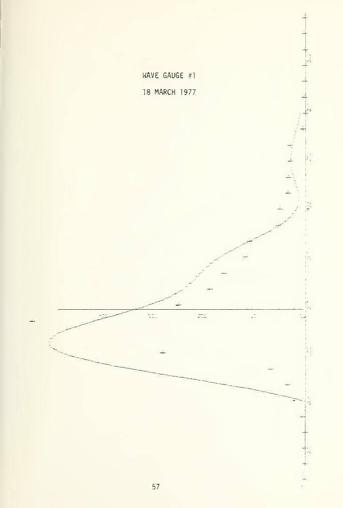
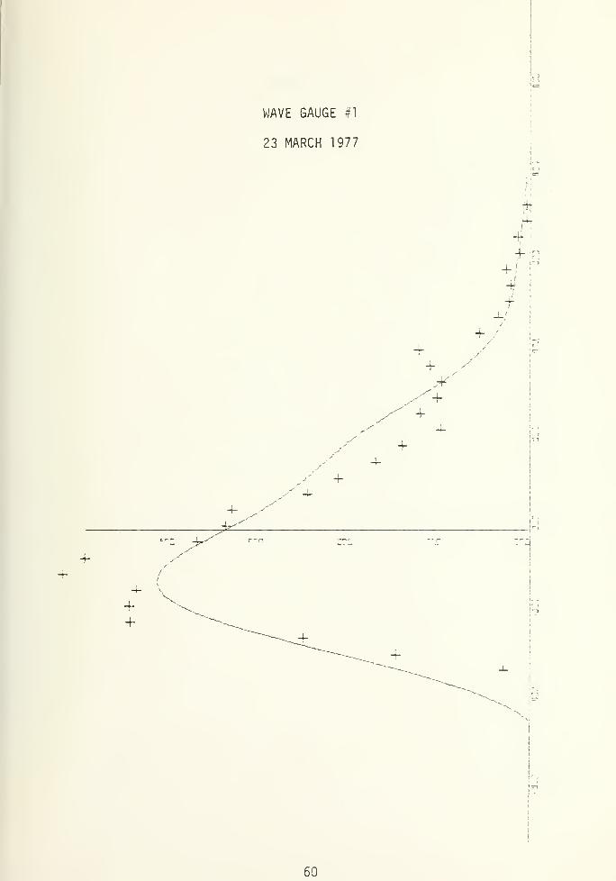
of Wave Gauge #1 on 23 March is shown in Figure 5. Appendix D contains

distributions calculated for other data sets.

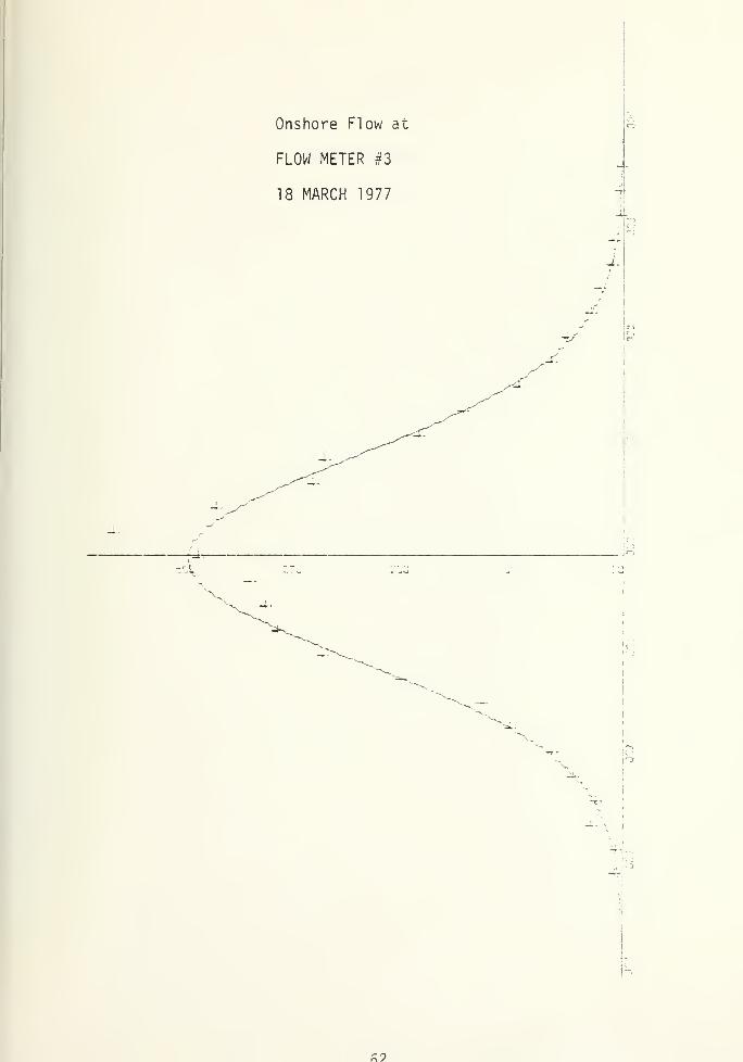
Distributions for all flow velocities are either unimodal or have

less pronounced secondary peaks compared to the distributions of wave

heights. The distribution of the onshore flow of Flow Meter #1 on 23

March is shown in Figure 6. As noted in Table II, this results in nearly

equal fit parameters with the Gram-Charl ier distribution being generally

smaller and thus a better fit. Fit parameters for velocity components

are much closer to zero than are the values calculated for wave components

since the flow meters do not experience the surface irregularities to

the same degree as do the wave gauges.

2. Skewness and Kurtosis

The sea surface distribution was found to be positively skewed.

This means that positive values are large, but less frequent than negative

values which are more frequent, but smaller, indicating a greater amount

of time below the mean water level. In other words, the crests are steeper

and more peaked, whereas the troughs are elongated and flatter which is

how waves in shallow water theoretically appear.

It should follow that the wave-induced particle velocities would

have distribution similar to the waves. However, of the 34 cases listed

in Table II, 17 had positive skewness and 17 had negative skewness with no

readily apparent pattern. Skewness of the onshore flow at Flow Meter #1

28

CT>

oi

—

o~> *rf •"=7 m if)

00 o~ r-j oc u3 co-»» CO CNJ a:i u"» 1

—

CT>

o .—

,

<3- o ui r»"i (VI

cc O rsj en «=T CD CO1

—

i~ . U> Oo o C3 rM U_J r— vO

a.1 .—

,

n: LXCi i «t U_l i

ex; 1 i i =3 1

—

1

cz i Cr _J ccr-> L_J 1 i i L/1 J- 4 UJ

,—

,

,—

t

i 1 ct *—/—

•

1 1 i i p—

*

Qi t —

1

C^ z X <t OHz <x. U-l Q o o~> uO o Cu 2£ <f.

•a: (_> CX •— 0A *—« <£ Xt_l 2» < f— UJ oo »~

<

CJu-> 1 <3. Q <c z- O uO 1

i/i s: —

•

2T >— 3 i

—

(£ 2C:z> «j' or <£ >» U_i ex: X ell

«-c a: <C (— U_l ^-' o < ex<_D CJ r> oO o on ^c CD L0

x:oto

O =w=Oaten=3IT3

cu>

C\J (TDO 3O-t->

Co+->

>O)

r— i

—

o UJo0)z <_>o <T3

1—

I

l»-

h— U<c 31—-t uo>UJ ra

cr Q (Vo ino Q cu

CX _c<£ 4->Q̂

4-<C Oh-oo C

o#— • 1—

o -(->o 31 J2)

C\J >.o c_>o cz1 CD

zz

crCDS_

i_=3en

4.0

C".o

cr

r^.r^cr.1—-Cm uO s_O fa

•z.

roC\J

co

,

—

=«=OJo s_c aj

+->

aj2:

son~u_

<

—

cr -Mcr fO

u~> 2z OO ^—4-

»—<£ at

s_

^> oLU JOO Q (/)

O co o

o CD

a; JO< +J

a4-

S: oi— |

—

C c/i cO oI

•r-4->

3-O

oo uc

cr

CD

cn

30

was always positive. Alongshore flow at the same location had negative

skewness in three of four cases. Onshore water particle velocity at

Flow Meter #2 had negative skewness for all six days. The skewness of

alongshore flow at the same point was positive in five of six cases.

The onshore component of flow at Flow Meter #3 had a positive skewness

for 16, 17, and 18 March and a negative skewness for the following three

days on which data was taken. Skewness of the alongshore flow at Flow

Meter #3 was positive for four of the six days. The reason for this

disparity is not known. Similar anomalous results have been found by

Thornton and Galvin (1975).

Kurtosis indicates the peakedness of each parameter. Just prior

to breaking the waves achieve the greatest degrees of peakedness. Visual

observations indicated that most of the waves were breaking at or near

Wave Gauge #1 on 17, 18, and 19 March; this correlates with their high

kurtosis values on these days. Values of kurtosis for all flow veloci-

ties again had no apparent pattern with values ranging from 2.6 to 8.6.

The reason for this is not known.

D. SPECTRAL ANALYSIS

1 . Sea Surface Elevation and Water Particle Velocity

The power, coherence, and phase spectra of Wave Gauge #1 and the

onshore component of the flow of Flow Meter #1 on 23 March are shown in

Figure 7. The spectrum of the wave surface elevation, which is char-

acteristic of all the records, show a narrow banded peak at a frequency

of 0.07 Hz, corresponding to a period of 14.3 sec. Also evident are

31

N

...I

CD «

LU

, n T

.MEASURED VELOCITY

.THEORETICAL VELOCITY

21L

LJ

Figure 7. Power, Coherence and Phase Spectra for the onshore flow of

Flow Meter #1 and Wave Gauge #1 on 23 March

32

peaks at 0.14 and 0.21 Hz which appear to be harmonics of the primary

peak at 0.07 Hz. These harmonics appear to be physical as was observed

from the strip chart earlier. The harmonics probably have some energy

contribution due to the Fourier computational technique. Appendix E

contains spectra calculated for all other wave and onshore flow data sets.

The coherence values were high, ranging to greater than 0.9 in

the maximum energy portion of the wave. Coherence begins to fall off

at about 0.5 Hz except on the 17th and 18th of March, the two days on

which short-crested waves were noted. On these days the coherence begins

to decrease at about 0.3 Hz. The decrease in coherence is probably due

to the relative increase in turbulence, the general decrease in energy

level, and wave energy spreading. The decrease in coherence due to wave

energy spreading is discussed in Section E.

The phase angle, which according to linear theory should be zero,

had an average value of less than 20 degrees over the highly coherent

band of prominent wave energy. The phase angle tends to increase slightly

over the coherent band and becomes random for the noncoherent region of

the spectrum.

In order to compare waves and flow velocity, the wave profile

spectrum was converted to a theoretical velocity spectrum for comparison

with the measured flow velocity spectrum using the linear transfer function

such that2

n

The transfer function is given from linear wave theory

V f) =l

H ( f H S~

(f) (2)

33

H(f) = 2 Trf coshk(h+z) (3)sinh kh

where

k is the wave number,

h is the mean water depth, and

z is the depth of flow meter below the mean depth (m)

Quantitatively, the results showed that linear theory overestimated

wave-induced velocity spectral components by about 50%; in previous

studies by Thornton et aj_ (1976) where the waves were long crested and

arrived at near normal incidence, the opposite was true, in that linear

theory underestimated the magnitude of the wave spectrum. The difference

in results is probably due to wave directionality, since when the wave

approaches at any angle other than normal the flow meter measures only a

component of the actual flow.

2. Onshore and Alongshore Flow

The cross-spectra between the onshore and alongshore components

of flow were calculated with the intent of finding the relation between these

two parameters. Power, coherence, and phase spectra of the onshore and

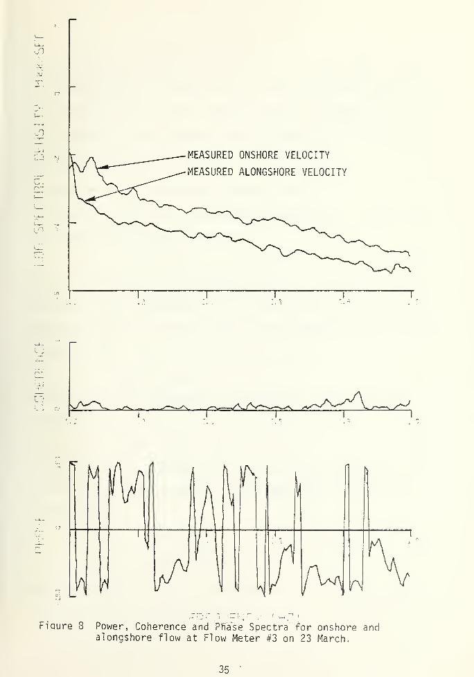
alongshore flows at Flow Meter #3 on 23 March are shown in Figure 8.

The spectra, which are representative of all the records, shows very

little coherence between velocity components. The phase angle is ran-

dom over the noncoherent band.

The reason for the lack of coherence between the two orthogonal

flow components is believed to be due to wave directionality. As was

seen earlier the onshore component of flow appears highly wave-induced;

34

v

JJMEASURED ONSHORE VELOCITY

MEASURED ALONGSHORE VELOCITY

Lj

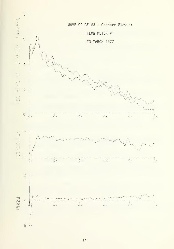
Fiqure 3 Power, Coherence and Pinase Spectra for onshore andalongshore flow at Flow Meter #3 on 23 March.

35

concomitantly, the alongshore flow component is at near normal incidence

to the wave direction and thus has only a small wave-induced contribution.

The variance of the alongshore component of flow is significantly less than

the on-offshore component except at zero frequency, which reflects the

mean longshore current variation.

E. TURBULENT VELOCITY VERSUS WAVE-INDUCED VELOCITY

The total velocity can be separated into components of a mean, plus

wave-induced, plus turbulent velocity

u = u + U + u1

. (4)

The wave-induced and turbulent velocity spectral components are assumed

to be statistically independent. For unidirectional waves aligned with

the measured velocity component, the co-spectra between waves and velocity

is then given by

V f >= W f) - (5)

Assuming statistical independence, the horizontal velocity spectrum

is obtained from

Su(f) = S

u,(f) + SjjCf). (6)

A further assumption is made that the waves and wave-induced velocities

are given by a constant parameter linear process where the coherence

is equal to unity

SU77(f)

*U f) = 1. (7)

VWf)Substituting (5), (6), and (7) into the definition of coherence between

the total horizontal velocity and waves results in

36

y (f)i fV(f)

SU (f)

l -1

= Mils (f) (8)

Increasing lack of coherence is due to an increasing high ratio of turbu-

lence. The coherence values indicate the percent of total velocity

which is associated with the wave velocity.

Wave-induced velocity can be determined using (8)

Sii(f) =y 2„>, (f)s„(f).

'U U77(9)

The wave-induced velocity spectral component calculated in this way

should be less than the actual value, the reason for this being that

the linear coherence between waves and velocities will always be under-

predicted due to nonl inearities which are always large in a breaking

wave and also as a result of directional spreading of the incident

wave energy (Battjes (1974) ).

The turbulent velocity spectrum is derived by subtracting the cal-

culated velocity spectrum from the measured velocity spectrum,

S.(f) = S„(f) - S„(f). (10)

The ratio of the turbulent velocity intensity to the wave-induced

velocities intensity is shown in Figure 9. The data used for collapsing

and plunging breakers, denoted by squares, was measured during earlier

studies by Thornton et al_ (1976). The collapsing and plunging breakers

were measured on beaches where the waves were long crested and arrived

at near normal incidence. The stars represent data collected during this

experiment. A value of the velocity intensity is given by taking the

37

iCVJ

1/1

ca;

oo

>

<UO

c7CD

en >03

a;

3-OS-3

14-

O

4->

<T3

a:

en

a-s-

3

38

square root of the variance which is computed by integrating the

velocity spectrum, S (f), across all frequency bands

The measurements show a small spread of values for the ratio of turbulent

to wave-induced velocity intensities. The average ratio calculated is

approximately 0.82. This would indicate that, to a first approximation,

the wave-induced kinetic energy is approximately 1.2 times the turbulent

kinetic energy. Thus the velocities in the surf zone on the average are

highly wave-induced.

If waves are not unidirectional, and generally they are not, it is

necessary to account for directional spreading. The wave angle striking

the wave staff and the type of wave, long or short crested, must be con-

sidered. In general, short crested waves predominated at Torrey Pines

Beach. On the 17th and 18th of March they were particularly noticeable.

The coherence between surface elevation and velocity components of short

crested waves is less than that of long crested waves due to directional

spreading. Using the wave train model developed by Yefimov and Khristoforov

(1971) the ratio of coherence between waves and onshore flow for the short

crested waves to that for long crested waves is given by

(12)

y2

utf>0s)(1 + V3ctn

2

£ o+ 4S

u,(f)/3S

u(f) )

_1

y^f.fli) (

i

+ su,(f)/s

u(f)[i/cos^ ] r 1

The model describes long crested waves using a train of two-dimensional,

planar random waves traveling in directionQ

. This corresponds to a

bivariate spectrum given by

39

^ (f,01) = Sn(f)6(<9-<9 ) , (13)

where 6(0-6o ) is the Dirac delta function.

Short crested waves appear as a train of three-dimensional waves

whose average direction of spectral components is assumed to be of the form

* (f,0s

)= { <

2/*> V f) cos2(0-*o) ,

n( for| - 0o\> tt II , (14)

Neglecting turbulence in order to examine the effect of directionality,

the ratio of the coherence between waves and wave-induced velocities for

short crested waves to that of long crested waves becomes

(15)

yltf,$s )+ l/3ctn

2^o)

_1

As an example, when 9 equals an angle of 30°, the ratio equals 0.9.

Conversely, the influence of turbulence on the ratio of coherence

between waves and velocities for short crested waves to that of long

crested waves can be examined by disregarding the directionality and

letting #o =0. The ratio is given by

rlMJs) - ( 1+ 4S ,(f)/3S

u(f) r 1

f-" y r . (16)

KrffW (] + s

u'(f ) /su

(f) )

A summary of the ratios considering the turbulence and/or direction-

ality factors at various angles is tabulated in Table III. The turbulence

factor, S /f )/Sy(f ) , is assumed for comparison purposes to be equal to

0.75, the average value for the measured data in Figure 9 as denoted by

the squares.

40

Table III

9 W^s'/'VV r>s>/ MV U?7 s UT) 1

(Equation 15) (Equation 16) (Equation 12)

0.875 0.875

5 0.997 0.877

10 0.990 0.882

15 0.977 0.891

20 0.957 0.905

25 0.932 0.923

30 0.9 0.947

The coherence between waves and velocities was used to calculate the

wave-induced velocity (equation 11). This method under-predicts the actual

wave-induced velocity because of nonlinearities and wave energy spreading.

Since the turbulent velocity is computed by subtracting the calculated

wave-induced velocity spectrum from the measured velocity spectrum

(equation 12) the smaller wave-induced velocity value makes the turbulent

velocity value larger. The average ratio of the turbulent velocity

intensity to the wave-induced velocity intensity was calculated to be

0.825. In order to correct for the directional spreading it is necessary

2 2

to multiply by the ratio 7 (f, B e )/y (f.0-,). As an example, the

ratio of the coherences for an angle of 15° is equal to 0.891. Multiplying

this value by the average ratio results in a turbulence to wave-induced

ratio of 0.75, which is equal to the earlier measured mean value. Hence

41

over the range of collapsing to spilling breakers a reasonable value for

a ' /a is approximately 0.75.

F. SATURATION REGION IN THE SPECTRUM OF BREAKING WAVES

Waves on Torrey Pines Beach characteristically broke as spilling

breakers with the crest sliding down the face of the wave. When the

fluid particles at the free surface move forward at a greater speed

than the wave speed, c, breaking occurs. Strong harmonics observed

in the wave and velocity spectra (Figure 7) are indicative of energy

being transferred from low to higher frequencies. The energy is even-

tually dissipated by viscosity at the highest frequencies. When the

transfer of energy is not rapid enough to balance the increase in energy

density of the waves during shoaling, breaking occurs. The waves are

said to be "saturated" with energy. Hence, a region of saturation

would be expected through which energy is transferred from the low to

higher frequencies. During shoaling and breaking of waves on a beach,

the waves become saturated at low frequencies first imposing a bound

on the peak energy density.

Spectra of waves at breaking, or just inshore of breaking, are

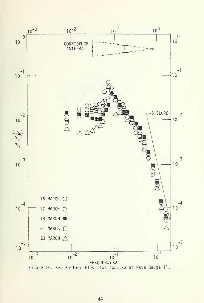
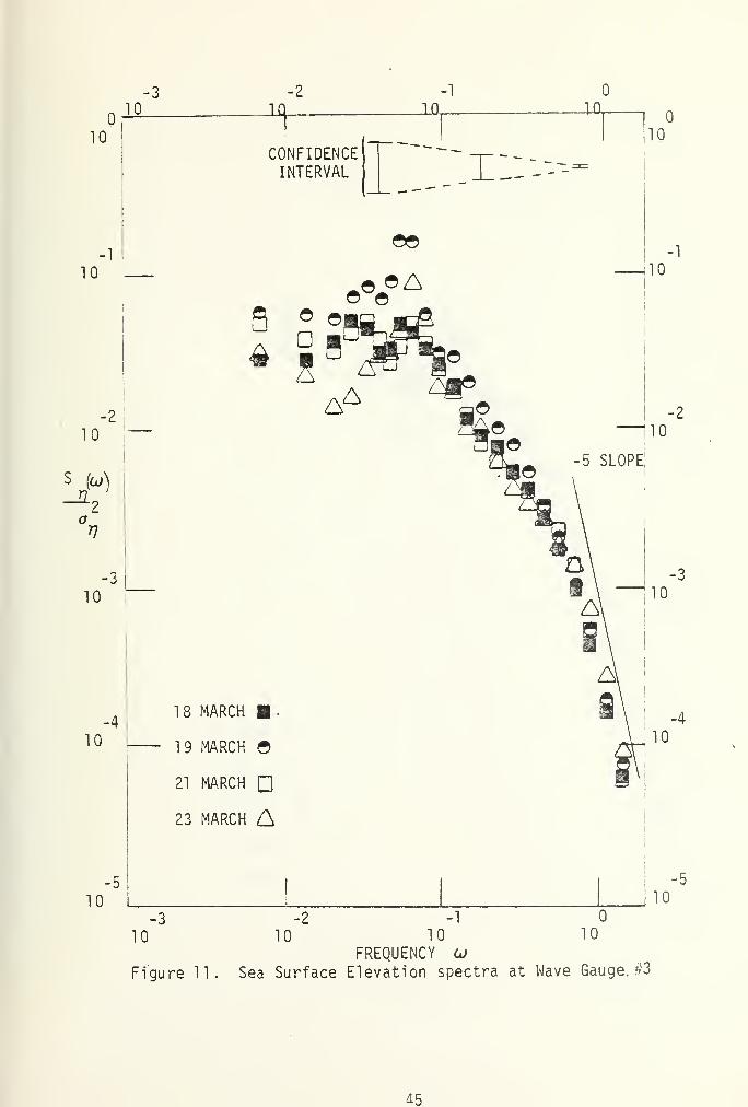
shown in Figures 10 and 11 plotted on a log-log scale. The spectral

estimates have been normalized by dividing by the total variance in an

effort to bring the high end of the spectra to a single line. The

spectral estimates have been block-averaged over frequency bands such

that the log-energy values are linearly distributed on the log-frequency

axis. The confidence intervals decrease with increasing frequency

because of the increasing number of frequency bands averaged over. The

42

confidence interval is noted on the figures. The slopes of the log-log

spectra at high frequencies for Wave Gauges #1 and Wave Gauges #3 can

be approximated by a -5 slope. This is indicative of a saturation or

equilibrium region for wind generated waves in deep water. This was a

surprise, as a -3 slope was expected for the waves measured in shallow

water, Thornton (1976). A possible explanation is that most of the waves

measured were waves inside the initial break point and would be classified

as spilling breakers or reformed waves. It may be that these types of

waves do not reach saturation condition as found for the more intense

plunging and collapsing breakers.

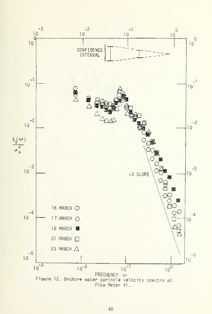
The normalized velocity spectra are given in Figures 12 and 13. The

slopes of the velocity spectra at higher frequencies at Flow Meter #1 and

Flow Meter #3 are both closely approximated by a -3 slope. A -3 slope

is expected for the equilibrium region in both deep and shallow water

and is consistent with the wave slopes.

43

10-3

10

-1

10

-2

10

*£

-3

10

-4

10-2

10-1

10l

CONFIDENCEINTERVAL i:~-----

A

10

-5

10

16 MARCH O17 MARCH O18 MARCH

21 MARCH Q23 MARCH A

-5 SLOPE

A

10

-1

10

-2

10

-3

10

10

-5

10^ ~1 A 1F

~10 10 10 10

FREQUENCY uFigure 10. Sea Surface Elevation spectra at Wave Gauge #1

.

44

10

-3

10

-1

10

-2

10

S (u)n

2

-3

10

-4

10

5-1

oa ao

CONFIDENCEINTERVAL

10

i::---

e©

-5

10

1

8

MARCH .

19 MARCH ©

21 MARCH

23 MARCH A

-1

10

-5

10

-3 -2 -1

10 10 10 10

FREQUENCY uFigure 11. Sea Surface Elevation spectra at Wave Gauge. #3

45

10Or

-2

10

-1

10

10

S (w)

-3

-4

10

-5

10

10-1

10 10

CONFIDENCEINTERVAL

10

~_i::-----

A iA

16 MARCH O1 7 MARCH O18 MARCH

21 MARCH

23 MARCH A

10

~3~,-2

10-

10

FREQUENCY uFigure 12. Onshore water particle velocity spectra at

Flow Meter #1 .

46

-3 -2

10

10

-1

10

-2

10

S Hu

7T

-3

10

10

CONFIDENCEINTERVAL

-4

10

-5

16 MARCH O

17 MARCH O

18 MARCH

21 MARCH D23 MARCH A

10

10-3 m" 2 10"

FREQUENCY uFigure 13. Onshore water particle velocity spectra at

Flow Meter #3.

47

V. CONCLUSIONS

The values of the pdf's of sea surface elevation were positively

skewed verifying the asymmetrical shape of the waves in the breaker zone.

On the other hand, the skewness of the velocity components were both

positive and negative and presented no readily apparent pattern.

The mean values of the onshore and alongshore components of flow indi-

cated the presence of a nearshore circulation cell probably associated with

the rip current which was frequently observed to the south of the instru-

ments.

The values of the velocity energy-density spectral components calculated

from wave spectra using linear theory indicate a qualitative, but not

quantitative, relationship. In general, linear theory overestimated the

magnitude of the velocity spectra because of wave directionality.

The high coherence between waves and onshore flow indicated that most

of the motion in the breaking wave is wave-induced. The coherence between

waves and onshore flow was used to separate the turbulence to wave-induced

velocity components. The measurements showed that over the range of col-

lapsing to spilling breakers a reasonable value for the ratio of turbulent

to wave-induced velocity is approximately 0.75.

The waves lead the onshore flow in spectral phase on the average

by less than 20 degrees, implying that the "curling" crest of the wave

arrives prior to maximum water particle velocity.

The wave and velocity energy-density spectra at higher frequencies

exhibited slopes of -5 and -3, respectively. This is indicative of deep

48

water wave conditions. A possible explanation for the surprising spectral

slope is that most of the waves measured were either spilling breakers or

reformed waves. It may be that the measured waves did not attain satura-

tion conditions during breaking, as do plunging and collapsing breakers.

49

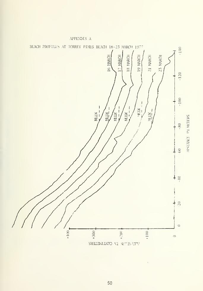
APPENDIX A

BEACH PROFILES AT TORREY PINES BEACH 16-23 MARCH 1977

c_j/ c_; U (J

o

SHHI3WIIN3D \'I NOIIVAHT?

50

oI—

I

I—

CD

<C_)

QQ LU

X Z3•— <

Q- << 3:

<Q-

/— CO=*fc =8=

<_3 CDZD ID

LU

-» <*>

C\J

CTi

CO

a:LU

U3

LO q_LUQ

-| ro

i- Jr 4 LC\J

CM

oCSJ

U3

(snoA) 39VH0A indino

T2T

o

51

APPENDIX C

CALIBRATION FACTORS

DATE INSTRUMENT

MARCH16,21,23 WG #1

17,19 WG #1

18 WG #1

ALL FM #1

DATESONSHORE

ALONGSHORE

FM #2

ONSHORE

ALONGSHORE

WG #3

FM #3

ONSHORE

ALONGSHORE

CALA* CALM**

-1 .154

-1 .284

-1 .453

.009

- .006

+ .131

- .084

- .2798

.007

.006

.00474

.00503

.00520

.00764

.00747

.00911

.00818

.00156

.00820

.00763

Calibration Additive Factor for wave heights is given in meters;CALA for flow is given in meters per second.

**Cali brat ion Multiplication Factor for wave heights is given in

meters per bit; CALM for flows is given in meters per second per bit.

52

APPENDIX D

PROBABILITY DENSITY FUNCTIONS VS

GRAM-CHARLIER DISTRIBUTIONS

f

7

rco

^fc 1

—

1^.

LU CTl

C3 r—ZD< IECD o

QiLU -<

v£>

_l.

+

i'

j-

53

Onshore Flow at

FLOW METER #1

16 MARCH 1977 r

i+:

/

+,

\ +4-

4----.

4*

A!

H\f

I

¥?

54

WAVE GAUGE #1

17 MARCH 1977

Onshore Flow at

FLOW METER #1

17 MARCH 1977

j

56

WAVE GAUGE #1

18 MARCH 1977

^

-+•

57

Onshore Flow at

FLOW METER #1

18 MARCH 1977

HP

-I-

f

H.

<£-

:-4

^x_

WAVE GAUGE #1

21 MARCH 1977

4

-/

4-

-i-

cu

!

59

WAVE GAUGE #1

23 MARCH 1977

tt

4f

4-

4l

4-:

4

+ .

y+^

4-

• 4-

/

+ /

4^4-

+

+

r-

60

WAVE GAUGE #3

18 MARCH 1977

1'i

-A.

f

"I\n

4-

-I

ll

61

Onshore Flow at

FLOW METER #3

18 MARCH 1977

T

'4-

*r

(-.

fi?

WAVE GAUGE #3

21 MARCH 1977

-k

-te

^'.

4-/ !

:

:

^

-A :

4-1

4-«

i

1"

63

I

1Onshore Flow at

FLOW METER #3

21 MARCH 1977

64

WAVE GAUGE #3

23 MARCH 1977 4

i4

ift

f+i

+!

65

Onshore Flow at

FLOW METER #3

23 MARCH 1977

4

/ i

66

\ \

APPENDIX E

POWER COHERENCE AND PHASE SPECTRA

WAVE GAUGE #1 - Onshore Flow at

FLOW METER #1

16 MARCH 1977

I \

\v v

\

v v

\A

\.-' Vj

Is- .*-

^V> , /V

nr

-1-^

i

67

J_

WAVE GAUGE #1 - Onshore Flow at

FLOW METER #1

17 MARCH 1977

,££>-,

'

68

WAVE GAUGE #1 - Onshore Flow at

FLOW METER #1

18 MARCH 1977

!

i /

.'i

;

69

/ 1

1 ,v. A

1 \

A

\ .

-\ -

w ><"»"S

WAVE GAUGE #1 - Onshore Flow at

FLOW METER #1

21 MARCH 1977

« r

i \

->a

i\

70

WAVE GAUGE #3 - Onshore Flow at

FLOW METER #3

18 MARCH 1977

;..'

c.

t

71

-x

r-

L2\

_J

rr

WAVE GAUGE #3 - Onshore Flow at

FLOW METER #3

21 MARCH 1977

% —^\i '/"-\.

^v ^y

*^Vv

'. 2 '. }

f/

-. /*\ /\j~ ^-*~1 / ^^- "v-—.—WW

! .

;

„ j' "V

h"

72

in

in

WAVE GAUGE #3 - Onshore Flow at

FLOW METER #1

23 MARCH 1977

HA

jj

">

vn^ \

^A

^

I. 3

"7"

i :T

lxy

r-J

V- .^" A

:.^

\)r-~ _. -

73

BIBLIOGRAPHY

Battjes, J., "Surf Similarity, 11

Proceedings of the Fourteenth Conferenceon Coastal Engineering , pp. 466-479, ASCE, 1974.

Bowen, A.J. and Huntley, D.A., "Field Measurements of Nearshore Velocities,Proceedings of the Fourteenth Conference on Coastal Engineering , pp.538-557, ASCE, 1974.

Bub, F.L., Surf Zone Wave Kinematics , M.S. Thesis, Naval PostgraduateSchool , Monterey, California, 1974.

Fuhrbbter, A., and Busching, F., "Wave Measuring Instrumentation forField Investigations on Breakers," Proceedings of the InternationalSymposium on Ocean Wave Measurements and Analysis , ASCE, 1974.

Galvin, C.J., "Wave Breaking in Shallow Water," Waves on Beaches andResulting Sediment Transport , pp. 413-456, Academic Press, Inc., 1972.

Galvin, J.J., Kinematics of Surf Zone Breaking Waves: Measurement and

Analysis , M.S. Thesis, Naval Postgraduate School, Monterey, California,1975.

Huntley, D.H., "Lateral and Bottom Forces on Longshore Currents," Pro-

ceedings of the Fifteenth Conference on Coastal Engineering , pp. 645-

659, ASCE, 1976.

Inman, D.L., and Nasu, N., Orbital Velocity Associated with Wave Actionnear the Breaker Zone , Technical Memorandum No. 79, U.S. Army Corpsof Engineers, Beach Erosion Board, March 1956.

Inman, D.L. and Kamar, P.D., "Longshore Sand Transport on Beaches,"Journal of Geophysical Research , V. 75, No. 30, October, 1971

Iverson, H.W., "Waves and Breakers in Shoaling Water," Proceedings of

the Third Conference on Coastal Engineering, Council on Wave Research ,

pp. 1-12, ASCE, 1952.

Khristoforov, G.N. and Yefimov, V.V., "Spectra and Statistical Relationsbetween the Velocity Fluctuations in the Upper Layer of the Sea and

Surface Waves," Atmospheric and Oceanic Physics , V. 7, No. 12, pp.

1290-1310, 1971.

McGoldrick, L.F., A System for the Generation and Measurement of Capillary-Gravity Waves , Technical Report No. 3, University of Chicago, Depart-

ment of the Geophysical Sciences, August, 1969.

74

Meadows, G.A., "Time Dependent Fluctuations in Longshore Currents,"Proceedings of the Fifteenth Conference on Coastal Engineering ,

pp. 660-680, ASCE, 1976.

Miller, R.L., and Ziegler, J.M., "The Internal Velocity Field in BreakingWaves," Proceedings of the Ninth Conference on Coastal Engineering , pp.

103-122, ASCE, 1964.

Steer, R. , Kinematics of Water Particle Motion within the Surf Zone ,

M.S. Thesis, Naval Postgraduate School, Monterey, California, 1972.

Thornton, E.B., "A Field Investigation of Sand Transport in the Surf Zone,'

Proceedings of the Eleventh Conference on Coastal Engineering , pp.335-351, ASCE, 1968.

Thornton, E.B., and Krapohl , R. F., "Water Particle Velocities Measuredunder Ocean Waves," Journal of Geophysical Research , v. 79, pp.847-852, 20 February 1974.

Thornton, E.B., and Richardson, D. P., The Kinematics of Water ParticleVelocities of Breaking Waves within the Surf Zone , Technical ReportNPS-58T 7401 1A, Naval Postgraduate School, Monterey, California,January 1974.

Thornton, E.B., "Review of Status of Energetics and Momentum Fluxes in

the Surf Zone: Field Data," Proceedings of the Workshop on CoastalSediment Transport Processes , University of Delaware, 2-4 December1976.

Thornton, E.B., Galvin, J.J., Bub, F.L. and Richardson, D. P. , "Kinematicsof Breaking Waves within the Surf Zone," Proceedings of the FifteenthConference on Coastal Engineering , pp. 461-476, ASCE, 1976.

Walker, J.R., Estimation of Ocean Wave-Induced Particle Velocities fromthe Time History of a Bottom Mounted Pressure Transducer , M.S. Thesis,University of Hawaii, 1969.

75

INITIAL DISTRIBUTION LIST

No. Copies

1. Defense Documentation Center 2

Cameron StationAlexandria, Virginia 22314

2. Library, Code 0142 2

Naval Postgraduate SchoolMonterey, California 93940

3. Department Chairman, Code 68 3

Department of OceanographyNaval Postgraduate SchoolMonterey, California 93940

4. Associate Professor E. B. Thornton, Code 68Tm 5

Department of OceanographyNaval Postgraduate SchoolMonterey, California 93940

5. LT A. J. Olsen 3

5806 N. 19th St.

Arlington, Virginia 22205

6. Oceanographer of the Navy 1

Hoffman Building No. 2

200 Stovall StreetAlexandria, Virginia 22332

7. Office of Naval Research 1

Code 410N0RDANSTL, Station, MS 39529

8. Dr. Robert E. Stevenson 1

Scientific Liaison Office, ONRScripps Institution of OceanographyLa Jolla, CA 92037

9. Library, Code 3330 1

Naval Oceanoqraphic OfficeWashington, D.C. 20373

10. SIO Library 1

University of California, San DiegoP. 0. Box 2367La Jolla, CA 92037

11. Department of Oceanography Library 1

University of WashingtonSeattle, WA 98105

7£

12. Department of Oceanography Library 1

Oregon State UniversityCorvallis, Oregon 97331

13. Director 1

Naval Oceanography and MeteorologyNational Space Technology LaboratoriesMSTL Station, MS 39529

14. NORDA 1

NSTL Station, MS 39529

15. Commanding Officer 1

Fleet Numerical Weather CentralMonterey, CA 93940

16. Commanding Officer 1

Naval Environmental Prediction Research FacilityMonterey, CA 93940

17. Department of the Navy 1

Commander Oceanographic System PacificBox 1390FPO San Francisco 96610

77

mtf

o^ie4^

\C5\o

Thesis0475

c.l

7272701 sen

The kinematics of

breaki ng waves i n

the surf zone.

thes0475

The kinematics of breaking waves in the

li

3 2768 001 97499 1

DUDLEY KNOX LIBRARY