The Jordan Econometric Macro Model (JEMM)

23 Jan 2013

This publication was produced for review by the United States Agency for International Development. It was prepared by DAI.

The Jordan Econometric Macro Model (JEMM) Jordan Macro Model (Revised Draft) 23 Jan 2013

i

The Jordan Econometric Macro Model (JEMM) Jordan Macro Model (Revised Draft)

2013-01-23

Program Title: Jordan Fiscal Reform II Project

Sponsoring USAID Office: USAID/Jordan Economic Growth Office

Contract Number: EEM-I-00-07-00009-00 Order No. EEM-I-08-07-00009-00

Contractor: DAI

Date of Publication: 23 Jan 2013

Author: Janusz Szyrmer

DISCLAIMER

The authors’ views expressed in this publication do not necessarily reflect the views of the United States Agency for International Development or the United States Government.

USAID-funded Fiscal Reform II Project, Jordan Macro Model Jan-2013 ii

CONTENTS

1. INTRODUCTION ............................................................................................... 1

2. MODEL CONCEPT ........................................................................................... 1

3. THEORY ............................................................................................................ 2

4. DATA ................................................................................................................. 2

5. EQUATIONS ..................................................................................................... 5

6. MODEL .............................................................................................................. 7

7. CONCLUSION ................................................................................................... 7

APPENDIX 1: MODEL SPREADSHEETS AND PROCEDURES ............................ 9

APPENDIX 2: MODEL VARIABLES ..................................................................... 12

APPENDIX 3: PROBLEMS WITH FOREIGN TRADE DATA ............................... 17

APPENDIX 4: PROBLEMS WITH GDP DATA ...................................................... 18

APPENDIX 5: RESULTS OF STATIONARITY TESTS OF THE VARIABLES USED IN REGRESSION EQUATIONS ............................................................................ 19

APPENDIX 6: TESTS FOR VIOLATIONS OF SELECTED OLS ASSUMPTIONS RELATED TO RESIDUALS OF REGRESSION EQUATIONS .............................. 21

APPENDIX 7: RESULTS OF TESTS FOR VIOLATIONS OF OLS ASSUMPTIONS22

APPENDIX 8: FLOW CHART PRESENTING THE RELATIONSHIPS AMONG MODEL’S BLOCS AND VARIABLES ................................................................... 23

APPENDIX 9: LISTING OF JEMM RELATIONSHIPS ........................................... 24

USAID-funded Fiscal Reform II Project, Jordan Macro Model Jan-2013 1

1. INTRODUCTION The Jordan Econometric Macro Model (JEMM) is intended to provide an initial simple structure to be used for macroeconomic forecasts as well as for impact simulations and policy analysis assessments for the Jordanian economy. It is based on quarterly data for 2000q1 – 2012q2 and generates forecasts for 2012q3 – 2014q4. The consecutive sections of this paper provide a brief overview of data used in the model and procedures for model creation: Concept, Theory, Data, Equations, Model, and Conclusion. More detailed technical information is provided in nine appendices, which document Model procedures, Variables, Data problems, Results of tests run on variables and regression residuals, and Relationships forming model’s equations. Appendix 8 contains a flow chart which presents the overall structure of the model. JEMM data and model’s results are contained in an Excel file “Jordan macro data 2013-01-22”. Regression equation and the model are generated by EViews 6: Eviews workfile : “Jordan macro model 2013-01-22”.

2. MODEL CONCEPT As indicated above, JEMM is intended to provide an initial simple structure to be used for macroeconomic forecasts as well as for impact simulations and policy analysis assessments for the Jordanian economy. Since concrete applications of the model are yet to be specified, JEMM is made as a “generic” construct, which will have to be adapted in order to become able to serve for more narrowly defined specific purposes of its future uses. While constructing JEMM, several standard model construction commandments were observed such: - Observe the Occam’s razor rule: keep the model parsimonious and avoid unnecessary

complications (the model contains simple OLS linear equations and simple identity/balance equations)

- Avoid data mining by as much as possible/feasible (theory-derived considerations support each equation included in the model)

- Avoid arbitrary interventions (such as the use of add-factors) and make the model as objective/neutral as possible

- Provide detailed documentation of the model to secure its verifiability/replicability and adaptability for diverse uses (this paper is intended to deliver such documentation)

The consecutive spreadsheets in the file “Jordan macro data 2013-01-22” (See Appendix 1), beginning with the sheet “Time Vars”, document the steps involved in the creation of JEMM (once its concept and theoretical foundations are defined): o “Time Vars”: “time” variables and dummies used in the model o “Mod Data”: Macroeconomic variables used in the model o “Mod Corr”: Pair-wise correlation coefficients among macroeconomic variables o “Mod Eqs”: Model equations o “Mod Res”: Model results, quarterly, for the entire model period, 2000q1 – 2014q4 o “ Mod Pred”: Model predictions, annual, for 2007-2014


3. THEORY Before a model is specified, one needs to formulate theoretical assumptions guiding its creation. JEMM is not based on any specific standard economic theory. As such it is somewhat eclectic. Overall, it follows a Keynesian school of thought: it is demand driven. The changes in aggregate demand, both internal and external, generate changes in aggregate output/ supply. Its underlying assumptions reflect general economic considerations for a widely open market economy, constrained primarily by governmental interventions which are limited mostly to price controls of currency (dollar-to-dinar exchange rate) and of prices of selected goods. Due to a relatively small size and the high level of openness of the Jordanian economy (which could be classified as an advanced emerging market economy), the external factors play a significant role in shaping up macroeconomic relationships and trends, and appear to be much more important than those in large advanced market economies. E.g., in the US there seems to be a much faster and stronger transmission of monetary policy instruments, such the effects of the changes of interest rates defined by the Federal Reserve. Also fiscal policy (tax collections and budget expenditure) seem to make a stronger impact on the domestic economy than fiscal policy in Jordan. The model could be extended/augmented by additional equations/modules to provide answers to more detailed questions (impact analyses of alternative policy scenarios).

4. DATA Data used in JEMM are derived from an Excel file “Jordan macro data 2013-01-22” (the sheets: E, G, M, P, R, and Time Vars). All together 55 quarterly macroeconomic variables, i.e., macroeconomic time series, are extracted, and defined in the model as either endogenous (49 variables), covering the period of 2000q1 – 2012q2, or as exogenous (6 variables), covering the period 2000q1 – 2014q4 (Appendix 2). Moreover 49 auxiliary variables were transferred from the Excel file (the sheet “Time Vars”) into EViews workfile, covering the period 2001q1-2014q4: “time” variable and 48 dummy variables. JEMM incorporates six “Rest of the world” (exogenously pre-determined) variables, which values are assumed to be independent from the trends occurring in the domestic Jordanian economy (Bloc 1). Also, there are 24 other External sector endogenous variables that remain under strong influence of the exogenous variables (Bloc 2). External sector’s closure requirements stipulate inclusion in the model of all main components of Balance of payments (Current account and its subcomponents, Financial account and its subcomponents, Capital account, and Errors & omissions) in order to satisfy the balance of payment requirements. Moreover, there are three domestic bloc data: Real sector and domestic prices (Bloc 3); Government (Bloc 4); and Banking (Bloc 5). These blocs are represented by much smaller numbers of variables. The role of domestic variables is not as big as the one in large advanced market economies. A number of factors are responsible for this. As emphasized above, the small size of the Jordanian economy and its emerging market status can partly provide explanation for this situation. Furthermore, the fix dinar-dollar peg reduces the effectiveness of instruments of the domestic monetary policy (such the interest rate). Similarly price subsidies and price controls diminish the role of domestic market signals sent to market participants by price changes. In addition, a number of noneconomic factors play an important role (Iraq war, “Arab Spring”, fiscal policy changes, etc.) affecting the economic causality relationships. This problem might be at least partially addressed by future modeling efforts. Yet another factor weakening economic relationships is data quality and availability. In particular, GDP quarterly data must be viewed as only rough approximations. Quarterly data and constant price data for Consumption, Investment, Employee compensation, Operating surplus, etc., are not


available and had to be estimated, which affects the reliability of model results. Import price indexes are incomplete (see Appendices 3 and 4). Due to a number of problems labor market data are not incorporated into the model (the data are incomplete and most of them provide annual figures only). More efforts are needed before they could be used in the model. The following variables are included in model’s blocs: Bloc 1: Rest of the world is represented by 6 exogenously pre-defined “E” variables: o Global economy, for which GDP of the USA is used as a proxy o Regional economy, represented by the average growth index of GDP of five Arab countries --

the main trading partners of Jordan: Egypt, Iraq, Saudi Arabia, Syria, and UAE o World market prices, approximated by two price indexes of crude oil and potash (statistical

tests have confirmed that these two variables had the strongest effect, direct and indirect, on Jordan’s export and domestic economy)

o Exchange rates, for which the JD-to-Euro exchange rate is used as a proxy o Capital account of the balance of payments (this is a relatively insignificant variable, needed to

be included for data consistency, i.e., for securing a perfect balance; for the prediction period it was assumed to be null)

Bloc 2: External sector consists of 24 “E” variables and 2 “P” variables: o Balance of payments (except Capital account), including Errors and omissions o Current account and its components o Financial account and its components o Real effective exchange rate: REER (no information is available how the rate is calculated;

there are two different time series for this variable and one of them was selected for JEMM) o Price indexes of goods: Export and Import Bloc 3: Real sector and domestic prices contains 6 “R” variables and 2 “P” variables: o GDP, Consumption, Investment o Employee compensation o Operating surplus (includes incomes of self-employed owners of small businesses) o Domestic price indexes: GDP deflator and Consumer price index Bloc 4: Government is represented by 11 “G” variables (only central government budget data are used as proxies for the consolidated budget of the public sector, since for the latter no quarterly data are available): o Revenue: Domestic revenue and Foreign grants (for the prediction period Foreign grants are

assumed to be equal to 10% of Jordan’s GDP) o Expenditure: Current and Capital o Budget balance: Before grants and After grants o Debt: Domestic and Foreign Bloc 5: The banking sector is composed of 4 “M” variables: o Interest rates (CBJ rediscount rate is used as a proxy) o Domestic time deposits o Domestic loans to private sector


o Domestic loans to public sector Additionally, a few annual variables are derived within the National balance bloc, which combines some External sector figures with Real sector figures, in order to calculate National disposable income, National savings, and National balance. Moreover in the model several auxiliary variables are used (imported from the sheet “Time Vars” in the data file), in particular: o “time“ variable:

time = 1, for 2001q1 time = 2, for 2001q2 Etc.

o 48 “Y” dummy variables: Outlier dummies specified for quarters with outlier observations

y1q1 = 1 for 2001q1, zero otherwise y1q2 = 1 for 2001q2, zero otherwise Etc.

Dummies identifying actual and predicted values of variables: yqact =1, for 2001q1, …, 2012q2, zero otherwise yqpred = 1, for 2012q3, …, 2014q4, zero otherwise

In the model, all variables which are expressed in the Jordanian dinars (JD m) are calculated in constant/fixed prices. The constant price variables are created by application of appropriate price indexes to their current/nominal price values, with the prices for the first year of the series (year =2000) used as their basis. The names of all constant price value variables are ending with the suffix “c”. The names of the variables consisting of time indexes (2000=100) are ending with the suffix “i”. Since almost all of the macroeconomic level variables are not stationary, i.e., they possess the “unit root” (time-varying parameters), it was decided to estimate the model directly on the first order difference values. Consequently, the values of the variables used in the model are first-order differences between the observations for a particular quarter and corresponding observations for the same quarter of a previous year. E.g., in the model, the constant price difference variable for GDP (r_gdpc) for 2001q1 was the difference between the constant price level value of GDP for 2001q1 and that for 2000q1: 91.32 = 1626.77 – 1535.45 (see sheet “Mod Data”, row 56 in the file “Jordan macro data 2013-01-22”) The differencing operation while reducing the number of observations for each variable by four (causing the loss of four degrees of freedom) generates the first-order differential time series with two convenient characteristics:

- The variables become de-trended, so the role of time trends driving the variables is greatly diminished. Only in a few cases the difference variables are still subject to a significant time trend. In these cases the second order differentials have to be derived (Appendix 5). E.g., the first order differential for dinar-euro exchange rate (exrate_euro) fails the stationarity test (at 10% significance level), but its second order differential (d(exrate_euro)) passes the test (at 1% significance level). All of variables, except one (Import prices) become stationary when second order differentials are applied.

- The effects of seasonality are completely removed from the data. No seasonal patterns were spotted in any time series used in JEMM.


5. EQUATIONS The model is composed of three kinds of equations: o 29 regression equations predicting the endogenous variables by applying regression

coefficients estimated by simple linear OLS specifications:

• Dependent variable = F(constant term and one or more independent variables)

• E.g.: Import of goods = F(Constant term, Export of goods, Private consumption, Investment, Time)

• In EViews: eim_goodstc c eex_goodstc r_consprivc r_investc time o 23 simple (additive) identities (balance equations) derived from definitions of the variables:

• Dependent variable = Sum of independent variables

• E.g., GDP = Sum of (Consumption, Investment, Net export)

• In EViews: r_gdpc = r_consprivc + r_consgovc + r_investc + enex_c o 3 conditional/behavioral identities reflecting model underlying assumptions:

Change in the stock of predicted foreign currency reserves is assumed to be equal to a product of the number of months of imports

• In EViews: eres_derc = eres_derc * yqact + yqpred * eres_monthsc * (-eim_c / 3)

• eres_derc = foreign currency reserves

• yqact = dummy: yqact = 1 for y1q1, …, y12q2, zero otherwise

• yqpred = dummy: yqpred = 1 for y12q3, …, y14q4, zero otherwise eres_months = reserve months (number of months of imports covered by foreign currency reserves)

• eim_c = value of imports of goods and services during one quarter (3 months) Number of predicted reserve months (in 2012q3 – 2014q4) is assumed to be growing by

two units every quarter, beginning the third quarter of 2012 In EViews: eres_monthsc = eres_monthsc * yqact + yqpred * 2 Foreign grants to budget during the prediction period are assumed to be equal to 10% of

GDP In EViews: grev_grantsc = grev_grantsc * yqact + yqpred * r_gdpc * 0.1

These assumptions are enforced in order to (1) maintain foreign currency reserves at a level assumed to be safe while keeping foreign debt at an adequate level; and (2) secure a greater inflow of foreign grants to budget (otherwise, the forecast, based on the trends during the last decade, would deliver a much lower level of the grants). Construction of regression equations involves unavoidable (sometimes highly arbitrary) decisions concerning:

- Selection of independent variables (predictors)

- Specification of lags for independent variables - Inclusion/exclusion of lagged dependent variables

- Inclusion of “time” variable and outlier dummies


- Differentiating one or more variables: first order differentials versus second order differentials (in JEMM all variables are either the former or the latter)

In making all these decisions one must consider performance of the regression equations according to different criteria (frequently conflicting one another), so in most cases several tradeoffs have to be addressed:

- Consistence with theory, which is not a simple “yes/no” consideration, especially, in dealing with direct relationships versus indirect relationships

• Say, when variable X depends on variable Y and variable Y depends on variable Z, the former relationship might be preferred to be included in the model over the latter relationship. However, when data suggest that the latter is more significant, then the model builder may prefer to include it into the equation. The question becomes by how much the latter relationship must be stronger than the former one in order for making this choice.

• For instance, in the economy, Domestic debt is directly related to Budget deficit, and only indirectly to Budget revenue, however in JEMM the latter is used as a predictor of Debt, because it generates better statistics, such as goodness of fit, significance of regression coefficients, etc.

- Simplicity

• The question is whether a simpler regression specification with one or two independent variables is better than another one with a much larger number of predictors. The former might be “cleaner” (more transparent) while the latter specification might be more cumbersome and weaker in terms of its econometric properties, e.g., suffering from multi-collinearity. However, larger number of predictors might significantly improve the goodness of fit and accuracy of predictions.

- Degrees of freedom

• This parameter is affected by numbers of observations and variables included in the equation. In general, the larger the number of the degrees the better, generating more robust estimates which are less affected by outliers (some of which might simply be data errors). Nevertheless other considerations, such as the need for using difference observations in order to make the series stationary, may lead to reduction of degrees of freedom, as it happens in JEMM.

- Period used for prediction

• In some situations, changing the period for equation estimation may generate more robust results and improve econometric properties of equations. This is especially the case, when the pattern of relationship significantly changes over time, and opting for specifying a shorter period which is free of unusual/unstable behavior of the variable might improve predicting capabilities of the equation.

- R-squared, F-stat, t-stats, and p-stats

• In general, specifications with high R-squared, high t-stats, low F-stats and low p-stats should be selected. However, other considerations may lead to different selections. E.g., one might be willing to include in an equation a variable with low a t-stat and high p-stat when no better predictors which are consistent with theory are available. For instance, in JEMM, in the equation predicting Government consumption, Budget revenue variable is included despite its low significance. The reason for this is the fact that in the equation Revenue is the only predictor linking the dependent variable to the rest of the economy.

• r_consgovc c grev_c(-1) r_consgovc(-1) - Violations of the OLS assumptions

• Removal of one violation may sometimes result in emergence of another violation. One has to decide which of the two violations is “less bad” (for instance, re-specifying an equation may get


rid of serial autocorrelation while making the residuals heteroskedastic). Also removal of a violation might greatly reduce the indicators of significance/goodness of fit or even almost completely “destroy” an equation and one may opt for tolerating the violation since generation of distorted estimates might still be viewed as a better choice than generation of no estimates. In construction of JEMM the equations were adjusted based on results of three tests of properties of residuals (Appendices 6 and 7).

- Problems with multi-collinearity

• This problem is especially acute when inclusion/exclusion of an independent variable leads to a large change of coefficient of another independent variable or even causes a change of sign of the coefficient (from plus to minus or from minus to plus) while both variables remain highly significant. One has to decide whether it is appropriate to keep both variables in the equation.

6. MODEL In EViews, “Model” is an “object” that generates solution to a system of simultaneous behavioral equations and identities. There are as many equations as unknowns for which the system is solved. All parameters incorporated in the simultaneous equations must be known (estimated from regressions runs prior to running Model). A large number of alternative specifications of JEMM’s equations have been tested, while the criteria of performance of equations and multiple tradeoffs have been considered and evaluated. Figure 1 (Appendix 8) presents the structure of the final model, being an outcome of these tests and considerations. In the figure the relationships among the variables are represented by two kinds of arrows: (1) thick arrows which show the inter-bloc relationships, i.e., those between the variables belonging to one bloc, defined as independent variables, and those belonging to a different bloc being defined as dependent variables; and (2) thin arrows which show intra-bloc relationships between the variables within each bloc. The relationships defining JEMM equations are presented in Appendix 9.

7. CONCLUSION Well in accordance with the Occam’s razor principle, it is good to begin policy research with a relatively simple model which later on can be extended for the needs of different concrete applications. Unlike some of previous macro modeling efforts, the Jordan Econometric Macro Model (JEMM) is intended to follow the Occam’s rule. It is relatively small and simple. As such it is not ready to be used to address concrete detailed policymaking issues. For these applications more work with data and model will be necessary. However, it has already provided some help in several areas, in particular: - Help in identifying data problems - Help in reconciling data and removing inconsistencies - Generating/estimating several important data series (especially GDP/Expenditure and

GDP/Income quarterly series, both in current prices and in constant prices that aren’t available in Jordan despite being of fundamental importance to economic policies in all advanced market economies)

- Providing a potentially useful learning tool about the Jordanian economy - Help in identifying and measuring selected important relationships, especially linear cause-

effect links and feedbacks, and in tracing effects of impacts, especially some longer term indirect relationships that are often intuitively not obvious, e.g., a very strong positive


relationship between loans delivered by banks to private sector and CBJ reference interest rate (there is a highly significant Granger causality between the CBJ rate and the loans)

- Generated initial forecasts to be considered in macroeconomic policy research, including warning signals for policymakers showing that according to JEMM’s predictions, based on 2000q1-2012q2 time series, in 2014 the current account deficit and budget deficit might become larger than currently, the national savings rate may shrink, loans to private sector may be crowded out by those to public sector, and both domestic and external debt may grow (these are obviously just initial results which are a econometric/mechanical extrapolation of the trends in the last decade and will require a further thorough scrutiny however they shouldn’t be ignored by policy experts)

Further work on data and modeling could enable the model to play an important role in policy analysis: - Potentially it may be used as a tax policy tool for estimating impacts of alternative tax reform initiatives.

- It may contribute to cost-benefit analysis of large investment projects.

- Also it may help in making comprehensive forecasts, both “warning” forecasts (what-if?) and ex-ante predictions.

Overall these kinds of macro models can help in capacity building in governmental organizations and NGOs. They can provide quantitative support for policy advocacy and transform policy debates from opinion-based (relying on intuition and conviction of debate participants) to facts-based. Efforts to quantify policymaking make policies less arbitrary, more transparent -- task oriented and evidence-based. As such they may help in reducing the influence of vested interests on policymaking and reduce opportunities for corruption. They may facilitate strengthening of fiscal and strategic planning (Medium term budget frameworks). They may become an important instrument for design and implementation of structural reforms; identification, measurement, and formulation of policies aimed at reducing macroeconomic distortions. They also provide useful instruments for a consistent policy benchmarking, continuous policy monitoring and evaluation. Last but not least, widely published good economic forecasts make the economy more transparent and more predictable, enhance “international image” of the country and may help its international ratings (such as investment ratings generated by Standard & Poor's, Moody, and Fitch) which in turn could help reduce the cost of credit and encourage domestic and foreign investors to spend money in Jordan. However to make all these accomplishments much more efforts must be spent on improving data, models, and strengthening their applications. International experience has demonstrated that the cost for practicing wrong macroeconomic policies is very high in political, social and economic terms as well as has confirmed the importance of proficient policy expertise and advice relying upon good macroeconomic statistics and strong analytical capabilities, including the area of model building covering diverse policymaking issues. In today’s globalized world, it would be difficult, if possible at all, to build a solid advanced market economy without developing these capacities.


APPENDIX 1: MODEL SPREADSHEETS AND PROCEDURES

Sheets “Time Vars” and “Mod Data” incorporate input data used for the model. In order to transfer the data into EViews the following steps are needed: In Excel (Sheet: Time Vars): o Highlight rows 2 through 50 and hit Ctrl-C

In EViews: o Select QUICK/EMPTY GROUP/TRANSPOSE (to create a group of time series organized by

the rows) o Click on < at the lower left corner of the sheet o Locate cursor in the top cell of the second column from the left (obs) o Copy data into EViews, as a group: Ctrl-V o You may use NAME to give a name to this group, e.g., “__time_dummies” o Quit group by hitting ‘x’ in the upper right corner

The sheet “Mod Data” contains macroeconomic time series selected for the model. There are 55 macroeconomic variables and 13 auxiliary variables used to check internal consistency of the data. E.g., checking consisting of GDP generates the following result: GDP – Consumption – Investment – Net exports = 0 This means that GDP values are consistent with the GDP/Expenditure definition. “Mod Data” is composed of the following data blocs: Columns H – S contain actual annual level observations of all macroeconomic variables, 2000-

11 Columns T – V contain predicted annual level observations for six exogenous variables, 2012-

14 Columns X – CE contain quarterly actual and predicted (exogenous) level observations,

2000q1 – 2014q4 The data used by the model are quarterly difference observations, for 2001q1 – 2014q4,

located in column CH (variable names) and columns CI – EL (variable values); each observation is equal to the difference between level observation for a particular quarter and level observation for the same quarter of previous year, so for each variable:

• Yiqj (difference) = yiqj(level) – yi-1qj(level), i = 2001, …, 2014; j = 1, 2, 3, 4 In order to transfer the data from Excel (sheet “Mod Data”) into EViews the following steps are needed: In Excel (Sheet: “Time Vars”):

o Highlight rows 4 through 58 for columns CH – EL and hit Ctrl-C In EViews:

o Select QUICK/EMPTY GROUP/TRANSPOSE (to create a group of time series organized by rows)

o Click on < at the lower left corner of the sheet o Locate cursor in the top cell of the second column from the left (obs) o Copy data into EViews, as a group: Ctrl-V o Use NAME to give a name to this group, e.g., “__data” o Quit group by hitting ‘x’ in the upper right corner


The sheet “Mod Corr” displays a matrix of pair-wise correlation coefficients between the 55 macroeconomic difference variables used by the model. These coefficients provide some suggestions as to which variables could potentially make good predictors for which time series, based just on numbers without accounting for theoretical considerations. These are purely “mechanical” indicators, nevertheless they are helpful in constructing model equations. The sheet “Mod Eqs” is a copy from “EViews MODEL/Equations” display. It incorporates both regression equations denoted as “Eqn” in column B of the sheet and identities denoted as “Text” in column B. The equations are listed in the alphabetic order of variable names. The sheet “Mod Res” contains model results. In EViews “Model” is a collection of equations, both regression equations and identities. “Model” doesn’t do any changes to the equation estimates (regression coefficients and other parameters). It simply solves an equation or a system of equations for the unknowns, e.g.: for the following equation it provides values for “y”:

y = c(1) + c(2)*x1 + c(3)*x2 + c(4)*x3 • where c(1), c(2), c(3), c(4), x1, x2, and x3 are known: x1, x2, and x3 are predictors; c(1), c(2),

c(3), and c(4) are coefficients estimated by a corresponding regression equation; and y is an unknown (dependent variable) to be predicted by this equation (for which this equation is solved).

Once all the equations are run and incorporated into the model, the model is ready to be run. When running the current specification of JEMM, Scenario 1 was selected and “Solution sample” was specified as 2012q3 – 2014q4 (forecast period). Model results were generated as new series with an extension “1”. Next all these variables were assembled in a “Group” named “__pred_1”. In order to copy them to Excel one should do the following: In EViews:

o Open group “__pred_1” o Press ‘Transpose’ o Press Ctrl-A and Ctrl-C, accept the default (‘Unformatted – Copy numbers at highest

precision’), and click on ‘Include header information’ In Excel (sheet “Mod Res”)

o Locate cursor in row 3/column G o Press Ctrl-V

• In the sheet “Mod Res” column G displays variable names and columns H – BK display variable observations, actual difference values for 2001q1 – 2012q2 and predicted difference values for 2012q3 – 2014q4 for all 55 variables. In columns BN – DV the actual values for level observations are derived from the difference values for the entire model period 2000q1 – 2014q4. Finally in columns DY – GH the level observations are calculated for current price values for all variables expressed in JD, by application of appropriate price indexes (actual and predicted, respectively).

In the sheet “Mod Pred” final results of the model are presented. In rows 4 – 70 the annual level observations are displayed: actual for 2007-2011 and predictions for 2012-14. They are organized into several blocs: Columns G – N: level observations in constant prices Columns Q – W: annual changes of constant price variables Columns Z – AG: level observations in current prices Columns AJ – AQ: current price variables expressed in JDs as ratios to GDP


Columns AS – AZ: consistency checks of observations for 2007-11, verifying that the final annual current price data (derived from constant price difference observations copied over back from EViews) are identical to the original numbers

In rows 74 – 87 National disposable income is derived from Real sector’s observations and External sector’s observations. Also National savings are calculated. These data are used to compile National balance in order to make sure that the data deliver a successful closure of the model by satisfying the balance conditions.


APPENDIX 2: MODEL VARIABLES

Variable Variable name Unit Predictors Comments EXTERNAL SECTOR 1 Balance of

payments E_bopc JD m Sum of:

Current account Financial account Capital account Errors & omissions

2 Current account ECA_c JD m Sum of: Export, goods & services, net Foreign factor income, net Foreign transfers, net

3 Export, goods & services, net

ENEX_c JD m Sum of: Export, goods & services Import, goods & services

Foreign trade balance

4 Export, goods & services

EEX_c JD m Sum of: Export, goods Export, services

5 Import, goods & services

EIM_c JD m Sum of: Import, goods Import, services

6 Export, goods, net ENEX_goodstc JD m Sum of: Export, goods Import, goods

7 Export, goods EEX_goodstc JD m Function of: World market prices, crude oil World market prices, potash Price index, export (-)

8 Import, goods EIM_goodstc JD m Function of: Export, goods (-) Consumption, private (-) Capital formation (Investment) (-)

Import takes on negative values, e.g., import of +100 becomes in the model -100. Predictors: aggregate demand variables

9 Export, services, net

ENEX_servc JD m Sum of: Export, services Import, services

10 Export, services EEX_servc JD m Function of: Export, goods Price index, export (-)

Export of services is negatively correlated with: Dinar appreciation: Exchange rate Real effective exchange rate Domestic price inflation: Price index: CPI Price index, GDP deflator

11 Import, services EIM_servc JD m Function of: Real effective exchange rate (-) Price index, import Import, goods Consumption, private (-)

See comment above for “Import, goods”.

12 Foreign factor income, net

EFFI_c JD m Function of: Credits to private sector GDP

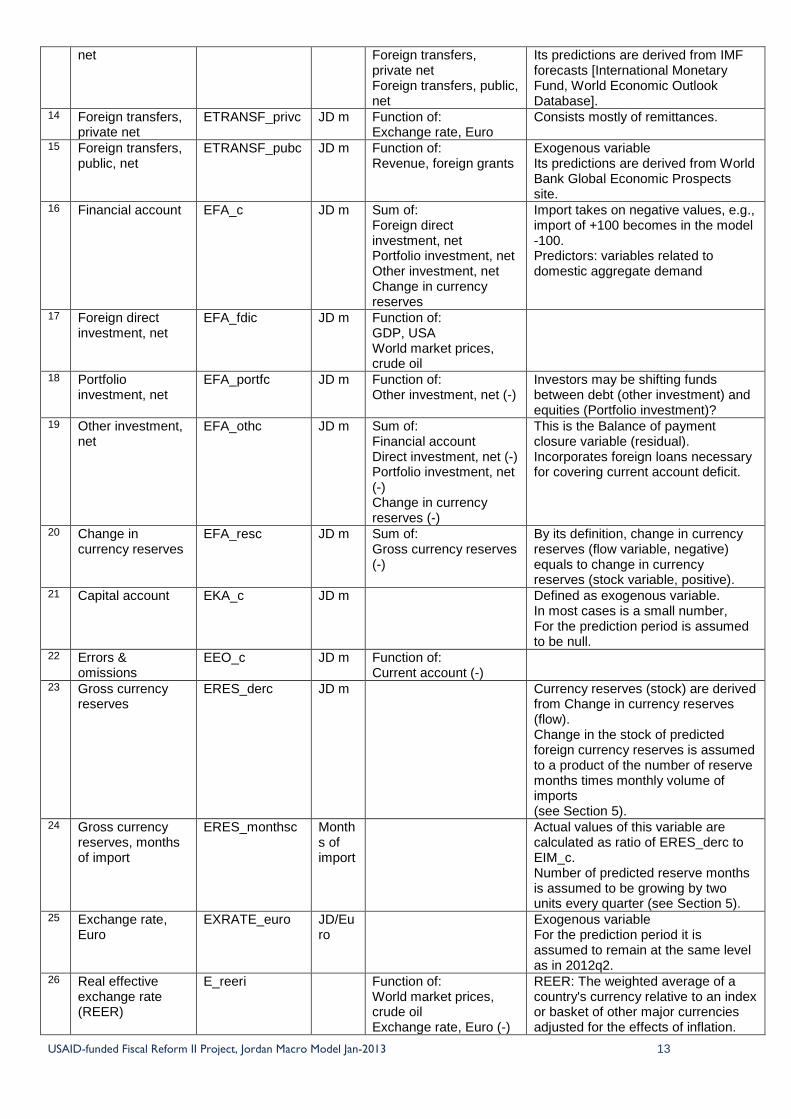
13 Foreign transfers, ETRANSF_c JD m Sum of: Exogenous variable


net Foreign transfers, private net Foreign transfers, public, net

Its predictions are derived from IMF forecasts [International Monetary Fund, World Economic Outlook Database].

14 Foreign transfers, private net

ETRANSF_privc JD m Function of: Exchange rate, Euro

Consists mostly of remittances.

15 Foreign transfers, public, net

ETRANSF_pubc JD m Function of: Revenue, foreign grants

Exogenous variable Its predictions are derived from World Bank Global Economic Prospects site.

16 Financial account EFA_c JD m Sum of: Foreign direct investment, net Portfolio investment, net Other investment, net Change in currency reserves

Import takes on negative values, e.g., import of +100 becomes in the model -100. Predictors: variables related to domestic aggregate demand

17 Foreign direct investment, net

EFA_fdic JD m Function of: GDP, USA World market prices, crude oil

18 Portfolio investment, net

EFA_portfc JD m Function of: Other investment, net (-)

Investors may be shifting funds between debt (other investment) and equities (Portfolio investment)?

19 Other investment, net

EFA_othc JD m Sum of: Financial account Direct investment, net (-) Portfolio investment, net (-) Change in currency reserves (-)

This is the Balance of payment closure variable (residual). Incorporates foreign loans necessary for covering current account deficit.

20 Change in currency reserves

EFA_resc JD m Sum of: Gross currency reserves (-)

By its definition, change in currency reserves (flow variable, negative) equals to change in currency reserves (stock variable, positive).

21

Capital account EKA_c JD m Defined as exogenous variable. In most cases is a small number, For the prediction period is assumed to be null.

22 Errors & omissions

EEO_c JD m Function of: Current account (-)

23 Gross currency reserves

ERES_derc JD m Currency reserves (stock) are derived from Change in currency reserves (flow). Change in the stock of predicted foreign currency reserves is assumed to a product of the number of reserve months times monthly volume of imports (see Section 5).

24 Gross currency reserves, months of import

ERES_monthsc Months of import

Actual values of this variable are calculated as ratio of ERES_derc to EIM_c. Number of predicted reserve months is assumed to be growing by two units every quarter (see Section 5).

25 Exchange rate, Euro

EXRATE_euro JD/Euro

Exogenous variable For the prediction period it is assumed to remain at the same level as in 2012q2.

26 Real effective exchange rate (REER)

E_reeri Function of: World market prices, crude oil Exchange rate, Euro (-)

REER: The weighted average of a country's currency relative to an index or basket of other major currencies adjusted for the effects of inflation.


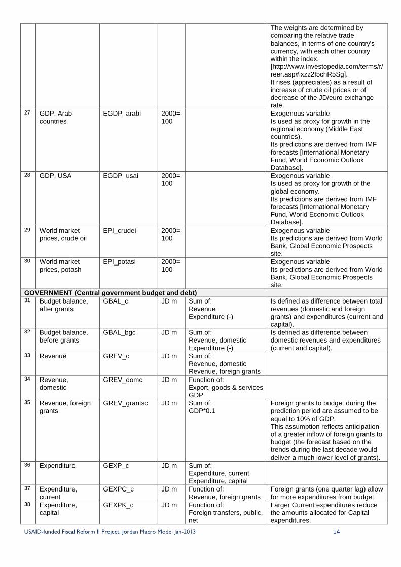
The weights are determined by comparing the relative trade balances, in terms of one country's currency, with each other country within the index. [http://www.investopedia.com/terms/r/reer.asp#ixzz2I5chR5Sg]. It rises (appreciates) as a result of increase of crude oil prices or of decrease of the JD/euro exchange rate.

27 GDP, Arab countries

EGDP_arabi 2000=100

Exogenous variable Is used as proxy for growth in the regional economy (Middle East countries). Its predictions are derived from IMF forecasts [International Monetary Fund, World Economic Outlook Database].

28 GDP, USA EGDP_usai 2000=100

Exogenous variable Is used as proxy for growth of the global economy. Its predictions are derived from IMF forecasts [International Monetary Fund, World Economic Outlook Database].

29 World market prices, crude oil

EPI_crudei 2000=100

Exogenous variable Its predictions are derived from World Bank, Global Economic Prospects site.

30 World market prices, potash

EPI_potasi 2000=100

Exogenous variable Its predictions are derived from World Bank, Global Economic Prospects site.

GOVERNMENT (Central government budget and debt) 31 Budget balance,

after grants GBAL_c JD m Sum of:

Revenue Expenditure (-)

Is defined as difference between total revenues (domestic and foreign grants) and expenditures (current and capital).

32 Budget balance, before grants

GBAL_bgc JD m Sum of: Revenue, domestic Expenditure (-)

Is defined as difference between domestic revenues and expenditures (current and capital).

33 Revenue GREV_c JD m Sum of: Revenue, domestic Revenue, foreign grants

34

Revenue, domestic

GREV_domc JD m Function of: Export, goods & services GDP

35 Revenue, foreign grants

GREV_grantsc JD m Sum of: GDP*0.1

Foreign grants to budget during the prediction period are assumed to be equal to 10% of GDP. This assumption reflects anticipation of a greater inflow of foreign grants to budget (the forecast based on the trends during the last decade would deliver a much lower level of grants).

36 Expenditure GEXP_c JD m Sum of: Expenditure, current Expenditure, capital

37 Expenditure, current

GEXPC_c JD m Function of: Revenue, foreign grants

Foreign grants (one quarter lag) allow for more expenditures from budget.

38 Expenditure, capital

GEXPK_c JD m Function of: Foreign transfers, public, net

Larger Current expenditures reduce the amounts allocated for Capital expenditures.


Expenditure, current (-) 39 Debt, gross GDEBT_gc JD m Sum of:

Debt, gross, domestic Debt, gross, external

40 Debt, gross, domestic

GDEBT_gdomc JD m Function of: Revenue, domestic (-) Credits to public sector Expenditure

Increased Revenue reduces Debt. Increased Expenditures augment Debt. Increased Public sector credits result in a higher Debt.

41 Debt, gross, external

GDEBT_gextc JD m Function of: Currency reserves Budget balance, after grants (-)

It is growing together with rising currency reserves. It is declining when budget deficit is shrinking.

MONEY AND BANKING 42 CBJ re-discount

rate MIR_cbj % Function of:

Foreign direct investment Domestic time deposits (-)

Here the direction of causality is unclear. Are the changes in the CBJ rate a reaction to increased FDIs and declining deposits or are the cause-effect relationships working in the opposite direction? Granger causality tests confirm causations in both directions expect the causation: Deposits=>CBJ rate.

43 Domestic time deposits

ML_timec JD m Function of: Price index: CPI(-) Compensation of employees

Growing inflation reduces real interest rates so it’s not surprising that the growing CPI is reducing the increases (or brings about decreases) in the deposits.

44 Credits to private sector

MA_privc JD m Function of: Domestic time deposits CBJ re-discount rate

As expected, Credits to private sector grow together with Time deposits (long term deposits). A solid positive relationship between the interest rate and credits might be explained by a growing eagerness of banks to provide loans when the rate is higher.

45 Credits to public sector

MA_pubc JD m Function of: Revenue, foreign grants(-) Expenditure, current Debt, gross, external(-)

Increased Foreign grants to budget and a growing Foreign currency debt allow for reductions of Domestic bank loans to government. Growing Budget expenditures contribute to Governmental domestic debt increases.

PRICES 46 Price index: GDP

deflator P_i 2000=

100 Function of: Price index, export Price index, import Consumption, government

The positive regression coefficients confirm that domestic price inflation in Jordan is predominantly “imported”.

47 Price index: CPI P_cpi 2000=100

Function of: Price index, GDP deflator Price index, export Price index, import World market prices, crude oil

See comment for “Price index, GDP deflator”.

48 Price index: export PE_exporti 2000=100

Function of: Price index, import

49 Price index: import PE_importi 2000=100

Function of: World market prices, crude oil GDP, USA

Increased oil prices and growth of the global economy stimulate increases of import prices.


REAL SECTOR 50 GDP R_gdpc JD m Sum of:

Consumption, private Consumption, government Capital formation (Investment) Export, goods & services Import, goods & services

GDP/Expenditure is calculated by its standard formula (as sum of final demand categories).

51 Consumption, private

R_consprivc JD m Function of: GDP Compensation of employees GDP, USA

Growing incomes of households enable Increases in Private consumption. A growing global economy (for which US GDP id used as a proxy) also has a positive impact on private consumption expenditure.

52 Consumption, government

R_consgovc JD m Function of: Revenue

Consumption of government does not enter into a significant relationship with any variable. Its relationship with Budget revenue is barely significant.

53 Capital formation (Investment)

R_investc JD m Function of: GDP, Arab countries Foreign factor income, net Foreign transfers, public, net Change in currency reserves Foreign direct investment, net Credits to private sector Price index, export

Changes in constant price Investment are derived from a regression equation. Changes in current price Investment are derived as a residual form an identity: Investment = GDP – Consumption – Net export Their nominal values behave erratically due to due to a lack of consistency in the actual GDP/Expenditure data.

54 Compensation of employees

R_compc JD m Function of: Function of: GDP Price index: CPI (-) Operating surplus (-)

Increasing price inflation tends to reduce real (constant price) labor income. A similar relationship occurs between the operating surplus (the “capital income”) and the compensation of employees (the labor income). This might be a manifestation of the labor-capital substitution.

55 Operating surplus R_surpc JD m Function of: Export, goods Price index, export GDP

Operating surplus tends to grow together with Export, Export prices, and GDP.


APPENDIX 3: PROBLEMS WITH FOREIGN TRADE DATA

There are three categories of exports: 1. Export of goods and services 2. Export of goods: domestic and re-exports 3. Export of goods: domestic There are three categories of imports: 1. Import of goods and services 2. Import of goods, including import by non-residents 3. Import of goods, excluding import by non-residents In our data only “Export of goods: domestic” and “Import of goods, including import by non-residents” are broken down into different commodity groups, so we have to use these two categories whenever we disaggregate Export and Import by commodities. Each combination of different categories of exports and imports gives different results when used for calculation of trends and modeling. The next problem is the derivation of export and import in constant prices from current/nominal price figures, which among other things enables us to analyze changes in the structure of the “real” economy, free of price change effects. The deflators for total export and total import published by DOS do not agree with the deflators derived from the sums of commodity groups in our database, deflated by group-specific price indexes. This creates some inconsistencies. In the data used for JEMM, the total Export/Import constant price values are produced by deflating the nominal price values with the price indexes derived from our macro database. This made our data internally consistent but inconsistent with the DOS indexes. Our new indexes for 2011 (218.0 for exports and 223.1 for imports) are significantly different from DOS indexes (233.9 and 296.6, respectively). Especially the large difference in import indexes may be a cause of concern. Furthermore there are several categories of export and import for which we don’t have price indexes, including:

• Other export • Other import • Re-export • Import by non-residents • Export and import by country • Export and import of services For services we could use either the GDP deflator or respective average price indexes (for total export and total import), or some other indexes. Depending on what we use we get (sometimes significantly) different results. Expanding our database will allow for securing a full consistency of trade data (it’s possible that more price indexes are available from DOS which would help in our data work).


APPENDIX 4: PROBLEMS WITH GDP DATA GDP data provide a cornerstone for a macroeconomic analysis and modeling. For the needs of JEMM, the GDP data published by DOS are used. Current problems with GDP include: 1. GDP/VA quarterly data display an unusual regularity and don’t correlate well with a number of

other important macroeconomic aggregates which are believed to be “hard data” (budget data, foreign trade, foreign investment, etc.); also their pattern significantly differs from the patterns of a number of other countries.

2. GDP/Expenditure are the most important macro aggregates: a. They aren’t consistent with GDP/VA for 2000-02. b. They aren’t up to date (we’ve got the data only through 2009 and even the 2009 data are

just preliminary). c. They are nominal only (in current prices); when we try to generate time series in constant

prices by applying available (corresponding) price indexes we aren’t getting reasonable results.

d. Government consumption data poorly correlate with the data on current expenditures of budgets of government agencies (central government, municipalities, government units, etc.); in fact they don’t significantly correlate with any other time series used for JEMM.

e. Investment data poorly correlate with other available investment time series (output of construction sector, public sector investment, foreign investment, donors’ projects, and imports of investment goods)

f. No quarterly data are available

3. There are similar problems with GDP-Income. GDP-Expenditure categories (household consumption, government consumption, private and government investments) are standard international macro statistics used widely by international organizations and are incorporated in all standard international data systems. Such indicators as changes in real household/private consumption, real investment, etc. are important data used in international economic/business reports and studies. It would be very useful to begin producing these data and keep them up to date by as much as possible.


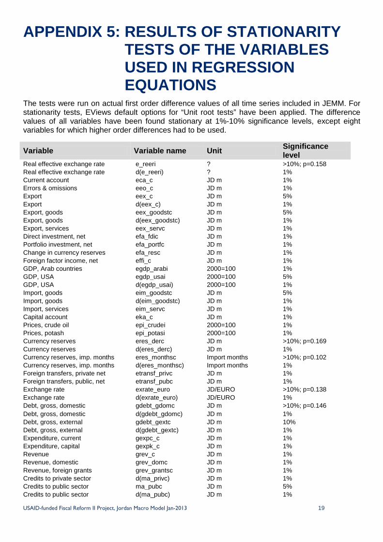
APPENDIX 5: RESULTS OF STATIONARITY TESTS OF THE VARIABLES USED IN REGRESSION EQUATIONS

The tests were run on actual first order difference values of all time series included in JEMM. For stationarity tests, EViews default options for “Unit root tests” have been applied. The difference values of all variables have been found stationary at 1%-10% significance levels, except eight variables for which higher order differences had to be used.

Variable Variable name Unit Significance level

Real effective exchange rate e_reeri ? >10%; p=0.158 Real effective exchange rate d(e_reeri) ? 1% Current account eca_c JD m 1% Errors & omissions eeo_c JD m 1% Export eex_c JD m 5% Export d(eex_c) JD m 1% Export, goods eex_goodstc JD m 5% Export, goods d(eex_goodstc) JD m 1% Export, services eex_servc JD m 1% Direct investment, net efa_fdic JD m 1% Portfolio investment, net efa_portfc JD m 1% Change in currency reserves efa_resc JD m 1% Foreign factor income, net effi_c JD m 1% GDP, Arab countries egdp_arabi 2000=100 1% GDP, USA egdp_usai 2000=100 5% GDP, USA d(egdp_usai) 2000=100 1% Import, goods eim_goodstc JD m 5% Import, goods d(eim_goodstc) JD m 1% Import, services eim_servc JD m 1% Capital account eka_c JD m 1% Prices, crude oil epi_crudei 2000=100 1% Prices, potash epi_potasi 2000=100 1% Currency reserves eres_derc JD m >10%; p=0.169 Currency reserves d(eres_derc) JD m 1% Currency reserves, imp. months eres_monthsc Import months >10%; p=0.102 Currency reserves, imp. months d(eres_monthsc) Import months 1% Foreign transfers, private net etransf_privc JD m 1% Foreign transfers, public, net etransf_pubc JD m 1% Exchange rate exrate_euro JD/EURO >10%; p=0.138 Exchange rate d(exrate_euro) JD/EURO 1% Debt, gross, domestic gdebt_gdomc JD m >10%; p=0.146 Debt, gross, domestic d(gdebt_gdomc) JD m 1% Debt, gross, external gdebt_gextc JD m 10% Debt, gross, external d(gdebt_gextc) JD m 1% Expenditure, current gexpc_c JD m 1% Expenditure, capital gexpk_c JD m 1% Revenue grev_c JD m 1% Revenue, domestic grev_domc JD m 1% Revenue, foreign grants grev_grantsc JD m 1% Credits to private sector d(ma_privc) JD m 1% Credits to public sector ma_pubc JD m 5% Credits to public sector d(ma_pubc) JD m 1%


Variable Variable name Unit Significance level

CBJ re-discount rate mir_cbj % 1% Domestic time deposits ml_timec JD m 1% Price index: CPI p_cpi 2000=100 1% Price index, GDP deflator p_i 2000=100 10% Price index, GDP deflator d(p_i) 2000=100 1% Price index, export pe_exporti 2000=100 1% Price index, import pe_importi 2000=100 >10%; p=0.441 Price index, import d(pe_importi) 2000=100 >10%; p=0.359 Price index, import d(pe_importi,2) 2000=100 1% Compensation of employees r_compc JD m 5% Compensation of employees d(r_compc) JD m 1% Consumption, government r_consgovc JD m >10%; p=0.480 Consumption, private r_consprivc JD m 1% GDP r_gdpc JD m >10%; p=0.196 GDP d(r_gdpc) JD m 1% Capital formation r_investc JD m 5% Capital formation d(r_investc) JD m 1% Operating surplus r_surpc JD m 5% Operating surplus d(r_surpc) JD m 1%


APPENDIX 6: TESTS FOR VIOLATIONS OF SELECTED OLS ASSUMPTIONS RELATED TO RESIDUALS OF REGRESSION EQUATIONS

*/ In order to try to fix the problems one may decide to re-specify the regression equations in the ways suggested in the column “Regression equation re-specification” of the table.

Violation of standard OLS assumption

Null hypothesis of test

EViews procedure

Result Comment Regression equation re-specification

Non-normality => the residuals are NOT normally distributed

H0: normal distribution of residuals

Run equation; View/Residual Tests/Histogram – Normality Test

In order to accept the NULL, p-stat has to be HIGH (0.1 or higher)

p-stat = the probability that a Jarque-Bera statistic ( its absolute value) exceeds the observed value under the null hypothesis; a small probability value leads to rejection of the null hypothesis

Try introducing outlier dummies for the highest/lowest residuals

Autocorrelation (serial correlation) => correlation of a variable with itself over successive time intervals

H0: no serial correlation of residuals => the dependent variable is NOT correlated with itself

Run equation; View/Residual Tests/Serial Correlation LM Test…./OK

In order to accept the NULL, p-stats for the F-test and/or for the Chi-Square test must be HIGH (0.1 or higher)

In EViews the default test for autocorrelation is the Breusch Godfrey Serial Lagrange Multiplier test

Try inserting into equation lagged dependent variable, quarterly and/or outlier dummies; replace dependent level variable with its first order or higher differencials

Heteroskedasticity => the residuals don’t have a constant variance

H0: Residuals are homoskedastic (possess a constant variance)

Run equation; View/Residual Tests/Heteroskedasticity Tests/OK

In order to accept the NULL, p-stats for the F-test and/or for the Chi-Square test must be HIGH (0.1 or higher)

In EViews the default test for Heteroskedasticity is the Breusch-Pagan-Godfrey test

See above


APPENDIX 7: RESULTS OF TESTS FOR VIOLATIONS OF OLS ASSUMPTIONS

The results of tests checking for violations of standard OLS assumptions concerning regression residuals: non-normality, serial correlation, and heteroskedasticity (see Appendix 6 for EViews procedures used for applications and the tests).

Regression equation Dependent variable Non-normality Serial

correlation Hetero-skedasticity

_e_reeri Real effective exchange rate No No No _eeo_c Errors & omissions No No Yes _eex_goodstc Export, goods No No No _eex_servc Export, services No No No _efa_fdic Foreign direct investment, net Yes Yes No _efa_portfc Portfolio investment, net No No No _efa_resc Change in currency reserves No No No _effi_c Foreign factor income, net No No No _eim_goodstc Import, goods No No No _eim_servc Import, services No No No _etransf_privc Foreign transfers, private net No No No _etransf_pubc Foreign transfers, public, net No No No _gdebt_gdomc Debt, gross, domestic No No No _gdebt_gextc Debt, gross, external No No No _gexpc_c Expenditure, current No No No _gexpk_c Expenditure, capital No No No _grev_domc Revenue, domestic No No No _ma_privc Credits to private sector No No No _ma_pubc Credits to public sector No No No _mir_cbj CBJ re-discount rate No Yes No _ml_timec Domestic time deposits No No No _p_cpi Price index: CPI No No No _p_i Price index, GDP deflator No No Yes _pe_exporti Price index, export Yes Yes Yes _pe_importi Price index, import No No No _r_compc Compensation of employees No Yes Yes _r_consgovc Consumption, government No No No _r_consprivc Consumption, private No No No _r_investc Capital formation No No No _r_surpc Operating surplus No No No


APPENDIX 8: FLOW CHART PRESENTING THE RELATIONSHIPS AMONG MODEL’S BLOCS AND VARIABLES

1. REST OF THE WORLD (EXOGEOUS VARIABLES)

Exchange rates

(Euro)

Global economy (USA)

Capital account

World market prices

Regional economy (Arab

countries)

2. EXTERNAL SECTOR

Real effective exchange rate

Foreign investment Foreign debt

Currency reserves

Export Import

Foreign factor income

Foreign transfers

Prices of goods: Export Import

Bal. of payments Errors &

Omissions

Current account

3. REAL SECTOR AND DOMESTIC PRICES

GDP deflator CPI

Operating surplus

Employee compensation

GDP Consumption Investment

4. BUDGET (CENTRAL GOVERNMENT) Domestic debt Foreign debt

Budget balance (deficit)

Budget expenditure

Budget revenue

5. DOMESTIC MONEY & BANKING

Public sector domestic loans

Private sector domestic loans

Bank domestic time deposits

Interest rates (CBJ)

Financial account


APPENDIX 9: LISTING OF JEMM RELATIONSHIPS Inter-bloc relationships

1. Rest of the world bloc’s variables are used as predictors for External sector variables and Real sector variables: o Index for World market price of crude oil is used as a predictor for REER, Export of goods,

FDI, Import prices, and CPI. o Euro exchange rate is contributing to predictions of REER and Private transfers

(remittances). o Potash price index contributes to predictions of Export of goods. o GDP of USA (a proxy for the performance of the global economy) serves as a predictor of

FDI, Prices of import of goods, and Private consumption. o GDP of the Arab countries serves as predictor of Investment (Capital formation).

2. External sector variables help make predictions of Real sector and domestic prices and Government sector: o Prices of export of goods and/or import of goods are used as predictors for Domestic prices

and Operating surplus. o Net export of goods and services is used for the derivation of GDP. o FDI, Foreign factor income, are Foreign public transfers are included in the equation

predicting Investment in Real sector. o Operating surplus is predicted by Export of goods and Export prices.

3. The variables of Real sector and domestic prices help predictions of External sector variables

and Government sector variables: o GDP serves as a predictor of Foreign factor income. o Private consumption and/or Investment are main predictors for Import of goods and Import

of services. o GDP is used as a predictor for Budget domestic revenue, and also as a base for deriving

Foreign grants to budget. 4. Budget variables are not highly correlated with other JEMM variables. They help predict only

two model variables (one from Real sector and one from Banking sector): o Real sector’s Government consumption is predicted by Budget revenue, although the

relationship is very weak. o As expected, Public sector bank loans are predicted by Budget expenditure, Foreign grants,

and Public external debt. 5. Domestic money and banking also plays a less significant role than in most other market

economies. It provides one independent variable for Government and another one for Real sector: o Domestic debt (stock) is predicted by Public loans (flow). o Private sector loans contribute to prediction of Investment.

Intra-bloc relationships

1. Rest of the world sector:


o Since all variables belonging to this bloc are exogenous they enter the model with pre-determined values and no relationships among them are accounted for.

2. External sector: o Errors and omissions are predicted by Current account values (under an assumption that

the former should change roughly proportionally to the latter). o Equations predicting Export of goods and Export of services include among their predictors

Export price index. o Export of goods serves as one of predictors for Export of services. o Foreign portfolio investment is predicted by Other foreign investment (mostly foreign loans). o Equation for Import of goods confirms the causality between Goods export and Goods

import, since production of exported goods calls for both domestic inputs and inputs from imports.

o In turn Import of services is dependent on Imports of goods (which have to be transported, insured, and serviced at least partly by foreign service providers), the exchange rate (REER) and Import prices.

3. Real sector and domestic prices: o GDP serves as a predictor for Compensation of employees, Private consumption, and

Operating surplus. o Compensation of employees (labor income) and Operating surplus (predominantly capital

income) enter a negative relationship (labor-capital substitution: the greater the Surplus the smaller the Compensation).

o An increased Compensation allows for increased Private consumption. o GDP deflator serves as a predictor for CPI. o CPI contributes to predictions of Compensation of employees.

4. Government: o Budget balances are derived from Revenue and Expenditures. o While Current expenditures depend on Revenues, Capital expenditures is negatively

related to Current expenditures (the higher the latter expenditures the lower the former expenditures).

o Domestic debt is related negatively to Revenue and positively to Expenditures. o Foreign debt in turn is negatively related to Budget balance after grants.

5. Banking: o As expected, Private sector loans are a function of Interest rates and Time (longer-term)

saving deposits (although somewhat unexpectedly, in the equation higher interest rates support the growth of the loans).

o Interest rates are negatively related with Time deposits (lower deposits on bank accounts are assumed to stimulate CBJ to increase the interest rate). However this relationship is not confirmed by a Granger causality test results.

Fiscal Reform II Project (FRP II)

Mecca Street, Nawfan Saoud Al Udwan St.

Abu Al Dahab Complex, Bldg 22- 4th floor

840126 Amman, 11181 Jordan

Phone: + (962 6) 592 2819

Documents

The Jordan Econometric Macro Model (JEMM)