Journal of Geophysical ResearchAccepted for publication, 1996

The Joint Gravity Model 3

B. D. Tapley, M. M. Watkins,1 J. C. Ries, G. W. Davis,2 R. J. Eanes,S. R. Poole, H. J. Rim, B. E. Schutz, and C. K. ShumCenter for Space Research, University of Texas at Austin

R. S. Nerem,3 F. J. Lerch, and J. A. MarshallSpace Geodesy Branch, NASA Goddard Space Flight Center, Greenbelt, Maryland

S. M. Klosko, N. K. Pavlis, and R. G. WilliamsonHughes STX Corporation, Lanham, Maryland

Abstract. An improved Earth geopotential model, complete to spherical harmonic degree and order 70, hasbeen determined by combining the Joint Gravity Model 1 (JGM 1) geopotential coefficients, and theirassociated error covariance, with new information from SLR, DORIS, and GPS tracking ofTOPEX/Poseidon, laser tracking of LAGEOS 1, LAGEOS 2, and Stella, and additional DORIS tracking ofSPOT 2. The resulting field, JGM 3, which has been adopted for the TOPEX/Poseidon altimeter datarerelease, yields improved orbit accuracies as demonstrated by better fits to withheld tracking data andsubstantially reduced geographically correlated orbit error. Methods for analyzing the performance of thegravity field using high-precision tracking station positioning were applied. Geodetic results, includingstation coordinates and Earth orientation parameters, are significantly improved with the JGM 3 model. Seasurface topography solutions from TOPEX/Poseidon altimetry indicate that the ocean geoid has beenimproved. Subset solutions performed by withholding either the GPS data or the SLR/DORIS data werecomputed to demonstrate the effect of these particular data sets on the gravity model used forTOPEX/Poseidon orbit determination.

Introduction

An Earth geopotential model, which has both high accuracy and spatial resolution, is arequirement for a number of contemporary studies in geophysics and oceanography. There hasbeen significant recent improvement in the accuracy of the Earth’s geopotential model, driven byoceanographic requirements for reduced errors both in the orbit of altimeter satellites and in thegeoid over the ocean basins [Tapley et al., 1994a]. The TOPEX/Poseidon (T/P) mission, whichwas launched in August 1992 as a joint project of NASA and the French space agency CentreNational d’Etudes Spatiales (CNES), contained the stringent requirement that the radial orbitaccuracy must be less than 13 cm RMS [Stewart et al., 1986]. Although the T/P satellite wasplaced in an orbit at an altitude of 1335 km to minimize the effects of atmospheric drag andgravity model errors, the prelaunch radial orbit error budget was dominated by a 10-cm root-mean-square (RMS) contribution from gravity field uncertainty [Tapley et al., 1990], and a majoreffort to improve the existing gravity models was initiated in 1983 as a joint effort between theNASA Goddard Space Flight Center Space Geodesy Branch (GSFC) and the University of TexasCenter for Space Research (CSR). This effort consisted of an iterative reprocessing of historicaltracking data from a number of satellites covering a range of orbit configurations in combinationwith new data from the satellite laser ranging (SLR) and Doppler orbitography andradiopositioning integrated by satellite (DORIS) tracking networks. The results of this effort ledto the Goddard Earth Model (GEM)-Tn and University of Texas Earth gravitational model(TEG)-n series of fields, detailed by Marsh et al. [1988, 1990], Tapley et al. [1989], Shum et al.[1990], and Lerch et al. [1994]. In addition, a group at the Ohio State University continued toexpand and improve the surface gravity database as described in Rapp and Pavlis [1990], Pavlisand Rapp [1990], and Rapp et al. [1991]. CNES provided data from the DORIS tracking system

1

carried on SPOT 2. The individual gravity model efforts were combined to develop the prelaunchgravity model for the T/P mission. The model, referred to as the Joint Gravity Model 1 (JGM 1)[Nerem et al., 1994], and based upon an accurately calibrated covariance [Lerch et al., 1981,1991], predicted a radial orbit error of 6 cm RMS. This value is well below the mission budgetallocation of 10 cm RMS and represents an order of magnitude improvement over gravity modelsavailable at the mission initiation, which predicted radial orbit errors exceeding 60 cm RMS. TheJGM 1 model represents a major improvement in the model for the Earth’s gravity field. Theachievement was possible only after extensive improvements in both the software and the modelsand in the tracking and surface gravity data. The model’s performance is evidence of the successof the efforts in these areas.

With JGM 1 as a starting point, information from the tracking of the T/P satellite itself wasused to improve the estimates of the linear combinations of coefficients to which the T/P satelliteis most sensitive. The complement of high precision tracking systems carried by T/P includes aretroreflector array for SLR [Degnan, 1985], a DORIS receiver [Nouel et al., 1988], and anexperimental Global Positioning System (GPS) receiver [Yunck et al., 1994; Melbourne et al.,1994], which provide both exceptional coverage and redundancy. This postlaunch modelimprovement, which led to the JGM 2 model, used only the SLR and DORIS data collected byT/P during a portion of the initial 6-month calibration/evaluation period [Nerem et al., 1994].

The radial orbit accuracy obtained for operational T/P precision orbit determination, using theJGM 2 gravity model, is in the range of 3 to 4 cm [Tapley et al., 1994a]. While this orbitaccuracy is considerably better than the JGM 1 orbit accuracy, there is evidence of gravity modelerror in the JGM 2 orbits. This conclusion follows from comparisons with high-precision orbitsdetermined with the GPS tracking of T/P [Bertiger et al., 1994]. Thus incorporation of the GPSdata can be expected to improve the gravity model further and reduce the T/P orbit errors,particularly those that are correlated geographically and are not reduced with temporal averaging[Tapley and Rosborough, 1985; Schrama, 1992].

Further evidence of error in the JGM 2 model is found by analyzing geodetic results from theLAGEOS-type satellites. The joint NASA/Italian Space Agency (ASI) LAGEOS 2 satellite, whichis a replica of LAGEOS 1, was launched in October 1992 into a 52.6˚ inclination orbit. The forceand measurement modeling errors for the two satellites should be very similar. However, whenseparate solutions for station position and geocenter (the absolute position of the SLR stationnetwork relative to the Earth’s center of mass) are performed by using JGM 2, there aredifferences in the results which are an order of magnitude larger than the expected errors.Combined satellite solutions for polar motion also display biases relative to the series determinedfrom each satellite alone. To achieve consistent results, it is necessary that selected geopotentialcoefficients be estimated as part of the multisatellite geodetic solutions, but the resulting solutionis not consistent with the original JGM 2 geopotential model. Similar results were noted in theDORIS station solutions obtained from SPOT 2 tracking data [Watkins et al., 1992; 1994]. Bothof these results indicate that there is significant gravity model error remaining in the JGM 2model.

New Satellite Tracking Data

The goal of this study was to combine several new data sets with the information in the JGM 1solution to determine an improved model for the Earth’s geopotential. This effort involved, first,the identification of tests accurate enough to distinguish improvements in the gravity field and,second, the use of these tests to define a strategy for combining the new data sets. JGM 1 wasadopted as the starting field rather than JGM 2 since this investigation processed a more extensiveset of SLR and DORIS data which was not available at the time JGM 2 was produced. TheJGM 1 and JGM 2 models differ only by the inclusion of SLR and DORIS tracking of T/P. Inaddition, to investigate the specific contribution of the T/P GPS data described below, it wasnecessary to start with a gravity model that did not contain a contribution from T/P.

2

The new data sets include the GPS data collected by the T/P GPS receiver, additional SLR andDORIS tracking of T/P, new SLR tracking of LAGEOS 2 and Stella, and additional SLR trackingof LAGEOS 1 and DORIS tracking of SPOT 2. Stella is a passive geodetic satellite designed tobe tracked by SLR for studies of the solid Earth. The high-inclination, nearly circular orbit andthe small area-to-mass ratio make the Stella data an important additional source of information forgravity model improvement. Additional details of these data sets are summarized in the followingdiscussion.

TOPEX/Poseidon

The T/P satellite consists of a large bus and a 28 m2 solar panel, with a total mass of 2500 kg.It occupies a nearly circular orbit with a 1330 km altitude and a 66˚ inclination. It carries twohighly precise radar altimeters and a microwave radiometer, in addition to supporting three precisetracking types [Fu et al., 1994; Tapley et al., 1994a]. A laser retroreflector array supports SLR asthe primary tracking system. The satellite is tracked by more than 30 sites around the world, withprecisions ranging from 5 to 50 mm. A DORIS receiver provided by CNES allows the satellite tobe tracked with Doppler range rate precisions that approach 0.5 mm/s from a well-distributedground network of more than 50 beacons. An experimental GPS receiver provides carrier phasemeasurements with 5 mm precision and pseudorange measurements with approximately 500 mmprecision, in the absence of antispoofing (AS). Because GPS tracking provides nearly continuous,high-precision, three-dimensional position information, it can be expected that the T/P GPS datawill provide considerable information for improving the low orders of the gravity model. Theground tracking network for these systems is illustrated in Figure 1. These data provide the firstopportunity for using the nearly continuous high-precision tracking provided by the constellationof 24 GPS satellites for precision orbit determination and gravity model improvement [Bertiger etal., 1994; Schutz et al., 1994; Tapley et al., 1995].

LAGEOS 2

LAGEOS 2 is a spherical spacecraft and a near-identical replica of the U.S.-launchedLAGEOS 1 satellite, with a mass of 407 kg and a diameter of 0.60 m. As a part of the jointNASA-ASI LAGEOS 2 mission the satellite was launched in October 1992 into an orbit with asemimajor axis of 5900 km, an eccentricity of 0.02, and an inclination of 52.6˚. The spacecraft’shigh altitude and low area-to-mass ratio attenuate the effects of the short wavelengths of thegravity field and surface forces. LAGEOS 2 is tracked by a global network of laser rangingstations. The single-shot precision of the best stations is a few millimeters. These stations havebeen used to obtain centimeter-level orbit accuracies for geodetic and geodynamic studies.

The motivation for including LAGEOS 2 in the new gravity field solution includes theimprovement of the estimates of the linear combinations of coefficients to which LAGEOS 2 isparticularly sensitive. These are dominated by the low degree and order coefficients for thisspacecraft. Furthermore, the geodetic parameters determined by analyses of LAGEOS 1 and 2depend upon the gravity coefficients for both improved orbit modeling and reference framedefinition. For polar motion solutions a linear combination of order 1 coefficients determines themeans of the resulting series. Thus, if the data from both LAGEOS 1 and LAGEOS 2 can beused to produce a gravity field with order 1 terms that are consistent for both satellites, then thepolar motion series determined by each of the individual satellites will have a consistent mean. Inaddition to the polar motion solutions, both the order one and resonance terms can also affect thedetermination of the tracking network origin with respect to the Earth’s center of mass, orgeocenter. Although the terms that define the mass center are actually of degree 1 and are nottraditionally adjusted, we have found that because of nonuniform tracking station distribution,some aliasing from low-degree order 1 terms, as well as resonance terms, is possible. Thecomputation of a gravity field model, which removes the problems described above, is aprerequisite for using LAGEOS 1 and 2 to determine accurate combined solutions for geodetic

3

parameters.

Stella

The Stella satellite was launched by CNES on September 23, 1993. The satellite wasconstructed as a copy of the Starlette satellite launched by CNES in 1975, but since it waslaunched concurrently with the SPOT 3, it is in an orbit very similar to that of both SPOT 2 andSPOT 3. Stella’s orbit has a semimajor axis of 7181 km, an eccentricity of 0.001, and aninclination of 98.7˚. The satellite has a depleted uranium core to decrease its area-to-mass ratioand, consequently, the effects of atmospheric perturbations at the 800 km altitude. Stella playstwo roles in the gravity model solution. As a withheld data set, it provides an excellent externaltest of the performance of existing fields, measuring primarily the treatment of the SPOT 2DORIS data, since it is in an almost identical orbit. As an easy-to-model spacecraft withoutmaneuvers, attitude uncertainty, or solar panels, it provides unique information for additionalgravity improvement. It is noted that, as with all Sun-synchronous orbits, errors in some of thesolar tides, particularly S 2, will be aliased into the estimates of the zonal coefficients. Since thetide model employed is based on a determination from a number of satellites without thisproblem, the aliasing effect will be small relative to the errors in the current zonal coefficients,and the resulting gravity solution will be an improvement.

Evaluation of Existing Gravity Fields

As a necessary condition for any improved Earth’s gravity field model, the orbit accuracyachieved for all satellites must be improved over the special models that have been developed forindividual satellites. The objective of the JGM model development effort, while directed to theparticular needs of the T/P mission, was to obtain a model that would yield the best accuracy onall satellites and, to the extent possible, improve the geoid. To a large measure, the long-wavelength components for the JGM 1 and 2 models [Nerem et al., 1994] represented the bestmodel for the majority of the existing satellites. However, as noted in the previous discussion,there are areas where these models require improvement.

Several tests can be applied to evaluate the accuracy of a given gravity field model. One testfor evaluating the model accuracy is the fit to tracking data on a specific satellite. The nature ofthe geographically correlated orbit error is another orbit performance test. A second test criterionis based on the stability and accuracy of the estimates of geodetic parameters, such as trackingstation coordinates and Earth orientation parameters, with tracking data from different satellitesusing a given gravity model. Results obtained with data not included in the gravity modelsolution lead to a more rigid test using either of these criteria. Finally, the accuracy of the geoidrepresents a third test. The evaluation of JGM 1 and 2 by these tests is described in thesubsequent discussion.

Tracking Data Residuals

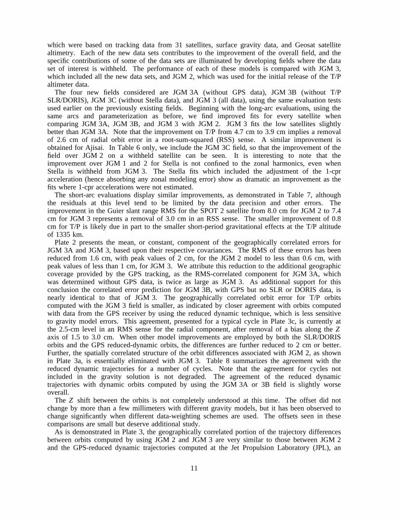
To obtain an accurate evaluation of the performance of a specific gravity field model on aspecific satellite, data spans of 3 to 5 days’ length with robust tracking and modest surface forceconditions were used. Generally, only the initial position and velocity, along with a dragcoefficient or a constant along-track acceleration parameter to account for unmodeled along-trackaccelerations, are estimated to ensure that the mismodeled zonal gravitational signal is notabsorbed. An exception to this philosophy was adopted for T/P. For this satellite, 10-day arclengths were used, and in addition to the parameters used for the shorter arcs, the coefficients fordaily once-per-revolution along-track and cross-track acceleration components were adjusted[Tapley et al., 1994a]. The data from these arcs have been processed by using the JGM 1 andJGM 2 gravity fields, and the results are presented in Table 1. This table is based on the SLRdata from a number of satellites in orbits with varying inclinations and altitudes. Data from the

4

Stella satellite are not included in either field, but the Stella orbit is very similar to that ofSPOT 2, which was included. With the exception of T/P and Stella, JGM 1 and JGM 2 yield thesame results. The improved performance on T/P with JGM 2 is expected, since the T/P data usedin the JGM 2 solution were not included in JGM 1. In Table 1, it can be seen that an additionaltest where one set of accelerations of 1 cycle per revolution (cpr) was included in the estimationprocess for Stella results in a significant reduction in the data fits. The 1-cpr parameters accountfor sinusoidal along-track and cross-track accelerations with a period equal to the orbital period(i.e., 1 cpr). These parameters effectively remove most of the secular and long-period orbit errordue to the error in the even and odd zonal harmonic coefficients and allow an accurate evaluationof the remaining portion of the gravity model. It can be seen that the fits for Stella areconsiderably poorer than those for any other satellite and that a significant contribution to theoverall RMS error can be attributed to errors in the zonal harmonics.

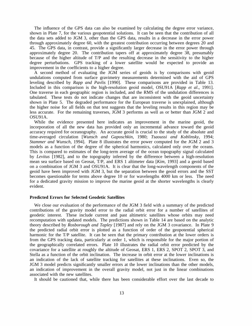
In addition to the longer arcs evaluated above, 8-hour arcs have also been assessed for the T/Pand SPOT 2 satellites by using the dense temporal coverage provided by the DORIS trackingsystem. The shorter arcs are less sensitive to the surface force effects and the long-periodgravitational perturbations, such as resonances. Consequently, they provide a means of evaluatingthe short-period gravity model errors. GPS tracking is the only other data source that wouldsupport such short arcs. For T/P an orbit determined by using the dense DORIS tracking data isalso evaluated by using SLR data for an estimate of the orbit error, while for SPOT 2, since thereis only DORIS tracking, a measure of the error is computed by using the Guier plane analysis ofGuier and Newton [1965]. In Table 2 it is shown that the short arcs for T/P are improved byusing JGM 2 compared to JGM 1, while the same level of accuracy is retained for SPOT 2.Table 2 also demonstrates that geopotential errors at this low level can be difficult to quantifystrictly on the basis of the data fits, since the changes in the RMS are in the second or thirdsignificant digit.

Geographically Correlated Orbit Error

The solution for the gravity field model contains both an estimate of the model parameters anda covariance matrix that describes the errors in the model. This error matrix can be used to maperrors in the gravity field model, as characterized by the error covariance, into uncertainties in thespacecraft orbit as a function of geographical location [Tapley and Rosborough, 1985; Schrama,1992]. The geographically correlated orbit error is a feature of all fields, although both themagnitude and the spatial structure will vary with the field. Furthermore, the structure willdepend on the specific satellite of interest. For dynamically consistent orbit determinationprocedures it is a particularly insidious error source, since this class of orbit error goes directlyinto the long-wavelength components of the sea surface topography derived from satellite altimeterdata and can be eliminated only by improving the gravity model. Plate 1 shows thegeographically correlated errors for JGM 1 and JGM 2 for T/P. The 2.5 cm mean amplitude ofthe geographically correlated error for JGM 1 has been reduced to 1.6 cm for the JGM 2 model.This improvement is attributable largely to the excellent geographical coverage of the DORIStracking system on the T/P satellite.

Geodetic Parameter Tests

One of the original requirements for accurate orbits resides in the need to determine accuratecoordinates of a set of globally distributed tracking stations. The determination of such points onthe Earth’s surface is also a requirement for tectonic plate motion studies. The accuracy oftracking site coordinates determined from analyses of satellite data has reached the centimeterlevel in recent years [Ray et al., 1991; Watkins et al., 1994; Himwich et al., 1993]. This accuracyallows the site coordinates to be used as sensitive diagnostics of parts of the gravity model.Specifically, the site coordinates are sensitive to the values of the terms of low degree and order,especially order 1, because of the dominant diurnal orbit signal associated with these terms. The

5

method used to evaluate a specific gravity field solution is to adjust the entire tracking network ina minimally constrained solution (typically a single longitude is fixed) by using observations froma single satellite. The results from this solution can be compared with the solutions generated bylong time series of SLR, very long baseline interferometry (VLBI), GPS, or the combination ofthese data sets. The approach is to fit a Helmert, or seven-parameter transformation, to the twonetwork solutions to determine the relative translations, rotations, and scale differences. Sinceeach satellite orbits the center of mass of the Earth, the translation parameters represent theconsistency in the determination of the center of the tracking network. The mass center of theEarth is known with a centimeter-level accuracy from analysis of LAGEOS 1 data. The rotationterms are essentially arbitrary. The scale differences are generally negligible when an accuratevalue for the gravitational mass (GM) of the Earth is adopted and the same tropospheric mappingfunctions are used in all solutions [Himwich et al., 1993]. The residual differences after theremoval of the common parameters are a measure of the relative positioning accuracy.

LAGEOS Station Comparisons

In this section the performance of the existing JGM 1 and JGM 2 fields is assessed bydetermining the effects on the relative station positioning and geocenter (i.e., translational errors inthe terrestrial reference frame) from LAGEOS 1 and 2. All station positions were computed byusing 3-day orbital arcs, 3-day Earth orientation parameter adjustments, and the adjustment ofrange or clock biases when necessary [Tapley et al., 1993]. The results demonstrate theinconsistency of the geocenters due to order 1 and resonance error in the JGM models.

Table 3 gives a comparison of LAGEOS 2 derived station positions to those obtained fromLAGEOS 1, using the JGM 1 and JGM 2 fields. Note particularly the geocenter offsets, which atup to 36 mm in the X coordinate, for example, are about 10 times larger than the expected levelof uncertainty. As mentioned earlier, this discrepancy is likely due to errors in the order 1 linearcombination for LAGEOS 2, which was not included in either of these fields. Table 1demonstrates that the performance of JGM 2 on the LAGEOS satellites is identical to that ofJGM 1 in terms of data fit and that orbit fits alone are an incomplete test of the gravity model atthis level of accuracy.

Table 3 also presents a comparison of the geocenter offsets obtained, for LAGEOS 1 only, byusing the JGM 1 field and another gravity model, the University of Texas Earth Geopotentialmodel (TEG) 2B [Tapley et al., 1991]. The primary difference is a 20 mm shift in the Xcomponent of the geocenter, which we interpret as being due to insufficient separation ofgeocenter and biases from the order 1 and resonance terms in the gravity model. This shift wasfirst recognized in early 1993, and consequently, the CSR 1993 laser ranging station solution(CSR93L01) was performed simultaneously with a selected gravity field adjustment [Eanes andWatkins, 1993]. The resulting solution indicated that both JGM 1 and TEG 2B had differences inlinear combinations of the geopotential coefficients that led to 10–15 mm errors in the Xgeocenter components. To remove the problem of geocenter error in the new field, additionalLAGEOS 1 data were combined with new LAGEOS 2 data, and partial derivatives for thegeocenter offsets and station-dependent biases were added to the estimated parameter array.

SPOT 2 Station Coordinates

Recent studies have shown that the positioning capability of the DORIS tracking system on theSPOT 2 spacecraft is at the few-centimeter level [Watkins et al., 1992, 1994a; Cazenave et al.,1992; Soudarin and Cazenave, 1995]. Thus the quality of the adjusted station coordinates can beused to discern the orbit errors due to the geopotential for this low-altitude satellite. In Table 4we present a summary of the relative differences between the estimated DORIS beaconcoordinates and a set of high-precision SLR and VLBI positions described by Watkins et al.[1994b]. The model, JGM 2*, in Table 4 is obtained by adjusting selected geopotentialcoefficients for each order between 0 and 29. This method gives a quick approximation of the

6

performance of a tuned field. The positions estimated with the DORIS data are significantlyimproved when the gravity model is allowed to adjust, even though very short arcs (8 hours) wereused in the station solution process in order to reduce the contribution of force modeling errors.On the basis of the results in Table 4 a reprocessing of the SPOT 2 data sets is warranted.

Description of New Information Equations

The techniques for creating the JGM 1 information arrays are summarized by Nerem et al.[1994]. The approach for combining the new information with the JGM 1 information isdescribed by Tapley et al. [1989] and Yuan [1991]. The standards and models used to process thenew tracking data are described by Tapley et al. [1994a] and are in large part consistent with theInternational Earth Rotation Service (IERS) standards of McCarthy [1992]. Specific detailspertinent to the individual data sets are given in the following.

LAGEOS 1 and LAGEOS 2

The information equations for the LAGEOS satellites were created by using arc lengths of 6days. The 6-day arc length was used to capture the 2.2-day period of the primary resonance forLAGEOS 1 and most of the 8-day resonance for LAGEOS 2. The nominal site positions andvelocities and Earth orientation series were from the CSR93L01 solutions. Within each 6-day arc,initial conditions and a constant tangential acceleration were adjusted. Partial derivatives for asingle adjustment of the gravity coefficients and geocenter were written. Solar reflectivitycoefficients were held fixed to values determined from previous long-arc solutions [Tapley et al.,1993]. The typical RMS for the reference orbits was 2.5 cm. The predicted RMS for this data setafter the geopotential adjustment was 1.9 cm. The data span was November 1987 through August1993 for LAGEOS 1 and October 1992 through August 1993 for LAGEOS 2.

Stella

All of the Stella data available at the time of the solution were used. They consisted of 30 daysof SLR tracking data from approximately 20 ground sites. The data were processed by using three10-day arcs in order to retain sensitivity to long-period resonance and secular zonal terms in thegravity field. Since such a limited data set was available and the primary goal was to improve thezonal harmonics, only a selected subset of the geopotential coefficients was adjusted with this dataset. This set included all coefficients up to degree and order 36, plus the resonance at order 43.Daily drag coefficients was estimated along with the initial position and velocity. The empirical1-cpr acceleration parameters was not estimated in order to avoid absorbing the secular and long-period signals from the errors in the zonal geopotential coefficients, since it was expected that thelow area-to-mass ratio of Stella would prevent the surface force modeling errors from being aserious limitation. The solar reflectivity is poorly separated from gravity coefficients because ofthe short data span, and this parameter was fixed to the value determined from multiyear Starlettesolutions. The site positions and velocities and Earth orientation series were fixed to theCSR93L01 values. The predicted RMS for this data set was 6 cm.

TOPEX/Poseidon GPS

The GPS data used for the gravity field adjustment consisted of cycles 10, 15, 17, and 19. Forcycles 10, 17, and 19, double-differenced measurements were formed by using two GPSspacecraft, one ground site, and the T/P spacecraft. For cycle 15 only, double-differenced phasedata between two GPS spacecraft and two ground sites were used in addition to the data formedfor the other three cycles. A 14-site subset of the 21-site GPS tracking network was used. Alldata were preprocessed at CSR, including editing and formation of double differences. Thedynamic and measurement models used are described by Schutz et al. [1994] and are generallyconsistent with the IERS standards for GPS. Selective availability (SA) was on during most of

7

the data collection intervals, although AS was off. The information equations were created byusing 3.3-day arcs for both T/P and the GPS spacecraft. Longer arcs produced degraded GPSspacecraft orbit accuracy, even with the adjustment of many dynamic parameters as well as thelarge parameter set resulting from the rigorous treatment of the ambiguities. The 3.3-day arcs,while short enough to allow good dynamic modeling, are long enough to capture the long-periodresonance effects. Daily 1-cpr empirical accelerations in the along-track and cross-track directionswere adjusted for both T/P and GPS.

The nominal T/P force and measurement models were derived from the T/P standards andincluded the macromodel of Marshall et al. [1994]. The measurement model used the dual-frequency GPS-derived ionosphere correction, and troposphere zenith delays were adjusted foreach site every 2.5 hours. Double-difference phase ambiguities were adjusted. Antenna phasecenter variations in azimuth and elevation for both T/P and the Rogue and TurboRogue groundsites using the choke ring antenna were modeled. In addition, the phase windup due to antennamotion was included [Wu et al., 1993], as well as the Doppler phase bias described by Bertiger etal. [1994]. The nominal Earth orientation series was CSR93L01, and all but one of the stationpositions were estimated. Finally, since preliminary comparisons of GPS- and SLR-derived orbitsfor TOPEX/Poseidon indicated an error of approximately 6 cm in the measured spacecraft centerof mass to GPS antenna offset in the spacecraft-centered Z coordinate (the radial component),partial derivatives for this parameter were also written. The typical predicted fit RMS for each3.3-day arc was 1 cm. Further details on the GPS data and its processing are given by Tapley etal. [1996].

TOPEX/Poseidon SLR/DORIS

Twenty repeat cycles of 10 days each were processed by using SLR and DORIS tracking data.The cycles spanned the period from cycle 1 through cycle 23, with cycles 10 and 11 omittedbecause of weak tracking. Other than a few minor exceptions, the force and measurement modelsadhered to the T/P standards described by Tapley et al. [1994a]. Ten-day arc lengths were usedfor the long-arc information equations including SLR and DORIS tracking. Daily tangentialaccelerations and 1-cpr along-track and cross-track accelerations were adjusted. The nominal SLRpositions and Earth orientation parameters were from the CSR93L01 solution, and the nominalDORIS site positions were based upon the SPOT 2 coordinates of Watkins et al. [1992]. Thepredicted SLR RMS was approximately 3.7 cm, while the predicted DORIS RMS was 0.51 mm/s.

SPOT 2

Two sets of SPOT 2 DORIS data have been processed at CSR for use in site positioning, orbitdetermination, and gravity field solutions. The first set consisted of 3 months of data covering theperiod from March 31, 1990, to July 5, 1990, and is characterized by numerous data gaps due tosatellite maneuvers and receiver interrupts. Only the uninterrupted 26-day span from May 3 toMay 29 was used for this solution. The data was processed in ten 2.6-day arcs, chosen to cover asignificant resonance. The drag coefficient was adjusted every 6 hours, and a single solarradiation reflectivity for the spacecraft body was adjusted for each arc. The nominal surface forcemodel assumed perfect yaw steering with main body areas of 6.5, 3.5, and 9.0 m2 in the roll,pitch, and yaw axes, respectively. The panel area used was 18.5 m2. Because of the reduced drageffects due to lower solar activity during this particular period, it appeared that estimating theempirical 1-cpr acceleration parameters could be avoided, and hence the zonal gravity informationwas retained.

The second set of DORIS data for SPOT 2 was 80 days of data collected during the so-calledAsymptotic Campaign from January 2 through March 23, 1992. Although this data set had fewerdata gaps than the 1990 set, it suffered from greater drag effects due to increased solar activity,despite its being temporally farther from the solar maximum. Consequently, it was necessary toadjust daily empirical 1-cpr accelerations in the transverse direction, in addition to the 6-hour drag

8

coefficients for the 2.6-day arcs. This same data set was also processed in the short arcs describedearlier, by using 8-hour arcs, with 4-hour drag coefficients, and a single 1-cpr along-trackacceleration. In addition, the pass-dependent wet troposphere zenith corrections and frequencyoffsets for the Doppler tracking were adjusted for both data sets.

Combination of New Data

In developing the new model the question of determining the proper relative weight of the newdata to the gravity field information arrays from the JGM 1 solution must be addressed. In thecomputation of JGM 2 a readjustment of all the relative weights for the information equations inthe JGM 1 model along with the weights for new T/P data were required. These weights,however, changed little from their values in the JGM 1 model [Nerem et al., 1994].Consequently, in our adjustment of JGM 1, the relative weights were fixed to the values assignedto the information arrays in the JGM 1 solution, and the relative weights of the new data sets weredetermined with respect to the JGM 1 solution. This procedure is equivalent to using the JGM 1coefficients and their associated error covariance matrix. This procedure differs from that used inthe computation of JGM 2 only when there are significant changes in the relative weights of theJGM 1 solution.

Effective Data Weight

In previous comprehensive gravity solutions performed at GSFC and CSR, relative satelliteweighting was performed by using algorithms for selecting the optimal values for the weights asdescribed by Yuan [1991] and Lerch [1991]. These approaches were not used in thisinvestigation, because software and methodology differences prevented incorporating the full set ofJGM 1 information equations. As an alternative, a parametric search for the optimal weights wasperformed by using a single data set. This weight was used for each new information equation.This parametric search was carried out by using information equations for SLR and DORIStracking of T/P, and gravity solutions were created by using various weights relative to JGM 1.The resulting fields were evaluated by using withheld arcs of tracking data for T/P and othersatellites as described in previous sections. The results of these tests indicate the need to weightthe data well below the weight implied by either the data precision or the data fits.

To understand this conclusion, some background on satellite data weighting is appropriate.When the data weight used in the creation of the information equations is correctly chosen, andthe residuals are purely Gaussian noise (with the data weight being equal to the inverse square ofthe standard deviation), the data set can be said to be correctly weighted, in the sense that thecovariance for the adjusted parameters will be statistically consistent with their errors. However,in the typical satellite problem the residuals are not Gaussian but are dominated by systematicerrors due primarily to gravity model errors, nongravitational surface force errors, andmeasurement model errors. Therefore the data noise variance is increased (the data weight isdecreased), so that the computed covariance will provide a realistic error estimate. This scalinginflates the noise-only covariance to approximate the effect of the various unknown modelingerrors. Although the magnitude of this increase depends to some extent on the satellite, for recent,well-tracked geodetic satellites the scaled data standard deviation is typically 10 to 50 times largerthan the random noise in the tracking data. This is also roughly 5 to 25 times the fit RMS. Forexample, SLR tracking of LAGEOS 1 was assigned an effective standard deviation of 1.12 m inJGM 1, when the RMS SLR noise, averaged over 1980–1988 (the span used in JGM 1), isapproximately 2–3 cm, and the RMS fit to the tracking data is better than 5 cm.

Returning to the description of our parametric search for appropriate weights, we note that, ifthe data noise used in the generation of the information equations reflects only the randomcomponent of the residuals, the optimal weighting scale factor should be between (1⁄50)2 = 0.0004and (1⁄5)2 = 0.04. The upper bound of this range agrees with our observation that the solutionsthat used weighting scale factors of 0.01 and 0.04 performed best. An additional solution was

9

also performed with a weight of 0.005, and the field was almost indistinguishable from fields withweights of 0.01 and 0.04. Therefore, while the optimal weights have not been determined in anyrigorous sense, the optimal weight is in a fairly "flat" region in the weighting space, and thesolution is not particularly sensitive to small changes in the weights. As a consequence of theseobservations an effective standard deviation approximately 30 times the data noise was used foreach satellite. The effective standard deviations are summarized in Table 5. The only exceptionsare the DORIS and GPS data, whose fits are much closer to the random noise because of the largenumber of measurement model parameters included in the solution. The standard deviations forthese data sets are increased by a factor of 15. It is reiterated that the weight of the JGM 1information array was fixed at 1.0; that is, the covariance of JGM 1 was assumed to be calibratedcorrectly. Comparisons of the differences between JGM 1 orbits and orbits computed with theimproved gravity models have verified that the JGM 1 covariance was in fact well calibrated.

Arc Length Philosophy

The perturbations on a satellite due to the geopotential can be classified as one of four basictypes: secular, long-period and resonance, m -daily or medium period, and short period [Kaula,1966]. The perturbations with periods longer than 1 day are the secular, long-period, andresonance perturbations. The resonance perturbations can often have periods of several days to afew weeks. The secular and long-period terms are due to the zonal harmonics (of even and oddparity, respectively), while the resonances are satellite dependent and generally occur at thesectoral terms for orders equal to a small integer times the number of revolutions per day. Theseterms cause the largest amplitude perturbations; however, they are actually small in number whencompared to the total number of geopotential perturbations. Most of the perturbations haveperiods that are less than 1 day, and the majority have periods less than 1 revolution. In contrastto the long-period perturbations, these short-period perturbations cannot be removed by adjustmentof satellite initial conditions when the arc length exceeds a few revolutions.

The improvement in the RMS fit to the tracking data as the arc length is shortened has beendemonstrated in Tables 1 and 2. The SLR range data for T/P using JGM 2 has an RMS residualof 4.7 cm for 10-day arcs, but a residual of 3.1 cm is obtained by using 8-hour arcs. In addition,as shown in Table 5, the determination of station positions on the Earth’s surface using DORISdata collected by SPOT 2, a satellite sensitive to short-wavelength gravity perturbations, improvedsignificantly when gravity coefficients were adjusted, even though an arc length of only 8 hourswas being used.

To achieve maximum sensitivity to short-period gravity perturbations, arc lengths of only a fewrevolutions are a logical option. There is the additional advantage that the effects of mismodelingthe nongravitational forces are substantially reduced by the frequent adjustment of the initialconditions, since surface force effects tend to build up secularly with time. However, short arcs ofa few hours’ length seriously degrade the observability of the large long-period, resonance, andm -daily terms for the lower orders. The accurate determination of these terms requires arcs of afew days’ duration. To address these two conflicting requirements, we have chosen the approachof using two information equations for the satellites with tracking dense enough to allow short-arcsolutions. One set of information equations is written by using arcs of a few days’ length todetermine the long-period terms, while another set with 8-hour arc lengths was used to increasethe signal-to-noise ratio for the short-period terms. Only DORIS and GPS provide the densetracking needed for the short-arc information arrays, and hence this approach could be used onlyfor SPOT 2 and T/P. However, the relatively high altitude of the T/P satellite attenuates theshort-period gravity signals, and hence short arcs were used only for the SPOT 2 spacecraft.

Evaluation of New Gravity Fields

On the basis of the previous discussion, new data from LAGEOS 1, LAGEOS 2,TOPEX/Poseidon, SPOT 2, and Stella have been combined with the JGM 1 information arrays,

10

which were based on tracking data from 31 satellites, surface gravity data, and Geosat satellitealtimetry. Each of the new data sets contributes to the improvement of the overall field, and thespecific contributions of some of the data sets are illuminated by developing fields where the dataset of interest is withheld. The performance of each of these models is compared with JGM 3,which included all the new data sets, and JGM 2, which was used for the initial release of the T/Paltimeter data.

The four new fields considered are JGM 3A (without GPS data), JGM 3B (without T/PSLR/DORIS), JGM 3C (without Stella data), and JGM 3 (all data), using the same evaluation testsused earlier on the previously existing fields. Beginning with the long-arc evaluations, using thesame arcs and parameterization as before, we find improved fits for every satellite whencomparing JGM 3A, JGM 3B, and JGM 3 with JGM 2. JGM 3 fits the low satellites slightlybetter than JGM 3A. Note that the improvement on T/P from 4.7 cm to 3.9 cm implies a removalof 2.6 cm of radial orbit error in a root-sum-squared (RSS) sense. A similar improvement isobtained for Ajisai. In Table 6 only, we include the JGM 3C field, so that the improvement of thefield over JGM 2 on a withheld satellite can be seen. It is interesting to note that theimprovement over JGM 1 and 2 for Stella is not confined to the zonal harmonics, even whenStella is withheld from JGM 3. The Stella fits which included the adjustment of the 1-cpracceleration (hence absorbing any zonal modeling error) show as dramatic an improvement as thefits where 1-cpr accelerations were not estimated.

The short-arc evaluations display similar improvements, as demonstrated in Table 7, althoughthe residuals at this level tend to be limited by the data precision and other errors. Theimprovement in the Guier slant range RMS for the SPOT 2 satellite from 8.0 cm for JGM 2 to 7.4cm for JGM 3 represents a removal of 3.0 cm in an RSS sense. The smaller improvement of 0.8cm for T/P is likely due in part to the smaller short-period gravitational effects at the T/P altitudeof 1335 km.

Plate 2 presents the mean, or constant, component of the geographically correlated errors forJGM 3A and JGM 3, based upon their respective covariances. The RMS of these errors has beenreduced from 1.6 cm, with peak values of 2 cm, for the JGM 2 model to less than 0.6 cm, withpeak values of less than 1 cm, for JGM 3. We attribute this reduction to the additional geographiccoverage provided by the GPS tracking, as the RMS-correlated component for JGM 3A, whichwas determined without GPS data, is twice as large as JGM 3. As additional support for thisconclusion the correlated error prediction for JGM 3B, with GPS but no SLR or DORIS data, isnearly identical to that of JGM 3. The geographically correlated orbit error for T/P orbitscomputed with the JGM 3 field is smaller, as indicated by closer agreement with orbits computedwith data from the GPS receiver by using the reduced dynamic technique, which is less sensitiveto gravity model errors. This agreement, presented for a typical cycle in Plate 3c, is currently atthe 2.5-cm level in an RMS sense for the radial component, after removal of a bias along the Zaxis of 1.5 to 3.0 cm. When other model improvements are employed by both the SLR/DORISorbits and the GPS reduced-dynamic orbits, the differences are further reduced to 2 cm or better.Further, the spatially correlated structure of the orbit differences associated with JGM 2, as shownin Plate 3a, is essentially eliminated with JGM 3. Table 8 summarizes the agreement with thereduced dynamic trajectories for a number of cycles. Note that the agreement for cycles notincluded in the gravity solution is not degraded. The agreement of the reduced dynamictrajectories with dynamic orbits computed by using the JGM 3A or 3B field is slightly worseoverall.

The Z shift between the orbits is not completely understood at this time. The offset did notchange by more than a few millimeters with different gravity models, but it has been observed tochange significantly when different data-weighting schemes are used. The offsets seen in thesecomparisons are small but deserve additional study.

As is demonstrated in Plate 3, the geographically correlated portion of the trajectory differencesbetween orbits computed by using JGM 2 and JGM 3 are very similar to those between JGM 2and the GPS-reduced dynamic trajectories computed at the Jet Propulsion Laboratory (JPL), an

11

indication that both the reduced dynamic solution and the new gravity field model remove most ofthe gravity model error in JGM 2, although through substantially different approaches. This is apowerful argument supporting both the improvement of the gravity model and the capability ofreduced dynamic filtering. Currently, since the errors from each technique are expected to be atthe 2.0 to 3.0 cm level, it is unclear whether this agreement can be improved significantly [Yuncket al., 1994; Tapley et al., 1994a].

To test the consistency of the linear combinations for LAGEOS 1 and 2, we repeat thecomparison for the independent site coordinate solutions from each satellite. Recall that thegeocenter differences are determined as the mean of the coordinates of approximately 50 SLRtracking stations, whose coordinates are determined by using LAGEOS 1 and LAGEOS 2 trackingdata to obtain two independent solutions. It is clear from Table 9 that the geocenter agreement isnow at the few-millimeter level in all three components, and at the 1 standard deviation level. Inaddition, the relative positioning is substantially improved, from the 10 to 20 mm level to lessthan 10 mm in each coordinate. The performances of JGM 3A and JGM 3 are virtually identical.

Table 10 demonstrates the improved performance of the new geopotential model on thepositioning for SPOT 2. By comparing Table 10 to Table 4 it can be seen that JGM 3outperforms the tuned JGM 2, for which selected geopotential coefficients were adjusted by usingSPOT 2 data. The performance of JGM 3A and JGM 3B was found to be nearly identical to thatof JGM 3.

The JGM 3 Geoid

In addition to the accuracy of the gravity model at satellite altitudes, the accuracy at sea level,as manifested in the determination of the marine geoid, is a topic of crucial interest for the area ofsatellite oceanography. The differences of the JGM 3 and JGM 3A geoids with respect to thegeoid of JGM 2 are presented in Table 11. The geoid difference between JGM 2 and JGM 3 isalso presented graphically in Plate 4. This figure demonstrates that the differences are largely overland, particularly over eastern Eurasia and South America, where the surface gravity data aresparse. The predicted errors in JGM 3, presented in Plate 5, indicate that the uncertainties are alsolargest at these locations. Table 11 shows that the addition of the GPS data changes the geoidover land at the 13 cm level, although over the ocean the change is approximately half that value.The predicted commission errors in the JGM 2 oceanic geoid (through degree 70) are at the 25-cmlevel, so the differences found in this study are reasonable.

While the changes in the geoid appear reasonable, it is difficult to assess whether they representan actual improvement over other models. We currently have evidence from two sources thatsuggest geoid improvement. The first is comparison of the satellite altimeter determined quasi-stationary sea surface topography (SST), derived by using the JGM 3 geoid, with the SSTdetermined from long-term in situ measurements such as those of Levitus [1982], which measuresprimarily the longer wavelength portion of the geoid. As described by Tapley et al. [1994b],SSTs from T/P referenced to the JGM 3 geoid are generally in better agreement with Levitus thanthose referenced to the JGM 1 or JGM 2 geoids. Table 12 demonstrates the results of acomparison for a 2-year mean SST determined with T/P altimeter measurements smoothed todegree and order 25. Data below −50˚ latitude are not compared because of errors in the Levitussurface due to lack of data. In addition to an overall reduction in RMS difference, specificfeatures in the SST referenced to the JGM 3 geoid appear to more accurately represent knownoceanographic features, such as the North Equatorial Countercurrent [Wyrtki, 1974; Tapley et al.,1994b]. This finding is demonstrated in Plate 6, where the 2-year mean SST inferred from theT/P altimetry is shown in relation to the JGM 2 and JGM 3 geoids. The "trough" that should beapparent in the equatorial Pacific region, due to the equatorial currents, is more distinct when theJGM 3 geoid is used. In Figure 2, the difference between the JGM 3 geoid and the geoidscalculated with JGM 3A and JGM 3B is presented. It can be seen that the GPS tracking data isthe primary contributor to the better definition of the geoid features in the equatorial region.

12

The influence of the GPS data can also be examined by calculating the degree error variance,shown in Plate 7, for the various geopotential solutions. It can be seen that the contribution of allthe data sets added to JGM 3, other than the GPS data, results in a decrease in the error powerthrough approximately degree 60, with the greatest contribution occurring between degrees 20 and45. The GPS data, in contrast, provide a significantly larger decrease in the error power throughapproximately degree 20. The contribution tapers off at approximately degree 38, presumablybecause of the higher altitude of T/P and the resulting decrease in the sensitivity to the higherdegree perturbations. GPS tracking of a lower satellite would be expected to provide animprovement in the coefficients to a higher degree.

A second method of evaluating the JGM series of geoids is by comparisons with geoidundulations computed from surface gravimetry measurements determined with the aid of GPSleveling described by Rapp and Pavlis [1990]. These comparisons are provided in Table 13.Included in this comparison is the high-resolution geoid model, OSU91A [Rapp et al., 1991].One traverse in each geographic region is included, and the RMS of the undulation differences istabulated. These tests do not indicate changes that are inconsistent with the geoid uncertaintyshown in Plate 5. The degraded performance for the European traverse is unexplained, althoughthe higher noise for all fields on that test suggests that the leveling results in this region may beless accurate. For the remaining traverses, JGM 3 performs as well as or better than JGM 2 andOSU91A.

While the evidence presented here indicates an improvement in the marine geoid, theincorporation of all the new data has provided only an incremental advance toward the geoidaccuracy required for oceanography. An accurate geoid is crucial to the study of the absolute andtime-averaged circulation [Wunsch and Gaposchkin, 1980; Tsaoussi and Koblinsky, 1994;Stammer and Wunsch, 1994]. Plate 8 illustrates the error power computed for the JGM 2 and 3models as a function of the degree of the spherical harmonics, calculated only over the oceans.This is compared to estimates of the long-term average of the ocean topography signal calculatedby Levitus [1982], and to the topography inferred by the difference between a high-resolutionmean sea surface based on Geosat, T/P, and ERS 1 altimeter data [Kim, 1993] and a geoid basedon a combination of JGM 3 and OSU91A. It is clear that the long-wavelength components of thegeoid have been improved with JGM 3, but the separation between the geoid errors and the SSTbecomes questionable for terms above degree 10 or for wavelengths 4000 km or less. The needfor a dedicated gravity mission to improve the marine geoid at the shorter wavelengths is clearlyevident.

Predicted Errors for Selected Geodetic Satellites

We close our evaluation of the performance of the JGM 3 field with a summary of the predictedcontributions of the gravity model error to the radial orbit error for a number of satellites ofgeodetic interest. These include current and past altimetric satellites whose orbits may needrecomputation with updated models. The predictions shown in Table 14 are based on the analytictheory described by Rosborough and Tapley [1987] and rely on the JGM 3 covariance. In Plate 9the predicted radial orbit error is plotted as a function of order of the geopotential sphericalharmonic for the T/P satellite. It can be seen that the primary contribution at the lower orders isfrom the GPS tracking data, particularly at order 1, which is responsible for the major portion ofthe geographically correlated errors. Plate 10 illustrates the radial orbit error predicted by thecovariance for a satellite at roughly the altitude of Geosat, ERS 1, ERS 2, SPOT 2, SPOT 3, andStella as a function of the orbit inclination. The increase in orbit error at the lower inclinations isan indication of the lack of satellite tracking for satellites at these inclinations. Even so, theJGM 3 model predicts significantly smaller errors at the lower inclinations than the other models,an indication of improvement in the overall gravity model, not just in the linear combinationsassociated with the new satellites.

It should be cautioned that, while there has been considerable effort over the last decade to

13

develop reliable estimates of the error covariance for the geopotential solutions leading up to andincluding the JGM series, the errors cannot be assumed to be Gaussian, and the error estimate forany particular coefficient may not be correct. Past experience, however, has demonstrated that thecovariance is quite accurate in predicting orbit errors for satellites not in the solution, such as theT/P error predictions using the JGM 1 covariance [Nerem et al., 1994].

Other Results

As was noted above, several parameters other than gravitational coefficients were adjustedglobally in the JGM 3 solution. These included geocenter adjustments to the CSR93L01 values,GPS site coordinates, and the GPS antenna center-of-mass offset in the spacecraft centered Z axisfor T/P.

The ground site coordinates for the GPS network were adjusted in a common fiducial freesolution simultaneously with the JGM 3 solution. The relative positions disagree with thenominal IGN93C02 coordinates at the level of 19 mm RMS. This result is obtained after theremoval of several sites whose coordinates indicate clear shifts from the nominal positions,primarily the site at Usuda, Japan, whose adjustment was near the meter level. Further, thetranslation parameters with respect to SLR-derived geocenter were at the centimeter level, afinding better than the agreement obtained by observing only the GPS satellites. Similar resultsare reported by Malla et al. [1993].

The JGM 3 solution for the T/P GPS antenna to center-of-mass offset correction was −5.3 cmwith an uncertainty at the millimeter level. This uncertainty is determined in the presence of afixed value for GM of the Earth of 398600.4415 [Ries et al., 1992]. The uncertainty in the valueof GM of about 2 parts per billion limits the true uncertainty of the observed radial antenna tocenter-of-mass offset to about 1 cm. The value observed was remarkably stable under a widevariety of changes in weighting and site coordinate adjustment.

Conclusions

A new model for the Earth’s geopotential, JGM 3, has been computed by combining theinformation from the JGM 1 solution with new and robust tracking of T/P, LAGEOS 2, andStella. In addition, some weaknesses of the JGM 1 and 2 models have been removed by theaddition of more data for LAGEOS 1 and SPOT 2. The new field provides significantimprovements in orbit accuracy as evaluated by tracking data fits and geodetic parameter recovery.In addition, the GPS tracking of T/P has significantly reduced the geographically correlated errorsin the gravity model. The JGM 3 model has been adopted for the rerelease of theTOPEX/Poseidon altimeter data, and the radial orbit error for the typical 10-day repeat period isreduced to approximately 2.8 cm RMS, with the geographically correlated orbit error reduced to 6mm RMS. We find that the T/P GPS data efficiently sense the gravity signal, with only four 10-day repeat cycles used to obtain gravity model improvement, comparable to 20 repeat cycles ofSLR and DORIS tracking. The geoid differences between the JGM 2 and JGM 3 models arewithin the expected uncertainties and are due primarily to the introduction of the GPS data. Theimproved geoid associated with the JGM 3 model yields more realistic ocean surface topographysolutions from T/P satellite altimeter data. Further, the continuous coverage provided by the GPStracking data improves the observability of nonresonant short-period gravity terms, which affectthe geoid but have little effect on the fit to tracking data and are thus difficult to assess. While webelieve that the geoid differences represent significant improvement, further study of this issue isrequired.

Acknowledgments. We gratefully acknowledge the support and contributions of the gravitymodeling and precise orbit determination teams at the University of Texas Center for SpaceResearch and the NASA Goddard Space Flight Center Space Geodesy Branch. We also thank theCentre National d’Etudes Spatiales and the Institut Geographique National for providing the

14

DORIS data and the associated station survey ties, and we thank the GPS demonstration receiverteam at the Jet Propulsion Laboratory for providing their GPS-based orbits. This research wassupported by NASA/JPL contracts 956689, 958122, and 958862.

References

Bertiger, W. I., et al., GPS precise tracking of TOPEX/Poseidon: Results and implications, J.Geophys. Res., 99(C12), 24449–24464, 1994.

Cazenave, A., J. J. Valette, and C. Boucher, Positioning results with DORIS on SPOT 2 after firstyear of mission, J. Geophys. Res., 97(B5), 7109–7119, 1992.

Degnan, J. J., Satellite laser ranging: Current status and future prospects, IEEE Trans. Geosci.Remote Sens., GE-32, 398–413, 1985.

Eanes, R. J., and M. M. Watkins, The CSR93L01 solution, in IERS Annual Report for 1992, Int.Earth Rotation Serv.,Obs. de Paris, 1993.

Fu, L.-L., E. J. Christensen, C. A. Yamarone Jr., M. Lefebvre, Y. Menard, M. Dorrer, and P.Escudier, TOPEX/Poseidon mission overview, J. Geophys. Res., 99(C12), 24369–24381, 1994.

Guier, W. H., and R. R. Newton, The Earth’s gravity field as deduced from the Doppler trackingof five satellites, J. Geophys. Res., 70(18), 4613–4626, 1965.

Himwich, W. E., M. M. Watkins, D. S. MacMillan, C. Ma, J. W. Ryan, T. A. Clark, R. J. Eanes,B. E. Schutz, and B. D. Tapley, The consistency of the scale of the terrestrial reference framesestimated from SLR and VLBI data, in Contributions of Space Geodesy to Geodynamics:Earth Dynamics, Geodyn. Ser., vol. 24, edited by D. E. Smith and D. L. Turcotte, pp. 113–120,AGU, Washington, D. C., 1993.

Kaula, W. M., Theory of Satellite Geodesy, Blaisdell, Waltham, Mass., 1966.Kim, M. C., Determination of high resolution mean sea surface and marine gravity field using

satellite altimetry, CSR Rep. 93-2, Cent. for Space Res., Univ. of Tex. at Austin, 1993.Lerch, F. J., Optimum data weighting and error calibration for estimation of gravitational

parameters, Bull. Geod., 65, 44–52, 1991.Lerch, F. J., C. A. Wagner, S. M. Klosko, and B. H. Putney, Goddard Earth models for

oceanographic applications (GEM 10B and 10C), Mar. Geod., 5(2), 243, 1981.Lerch, F. J., J. G. Marsh, S. M. Klosko, G. B. Patel, D. S. Chinn, E. C. Pavlis, and C. A. Wagner,

An improved error assessment for the GEM-T1 gravitational model, J. Geophys. Res., 96(B12),20023–20040, 1991.

Lerch, F. J., et al., A geopotential model for the Earth from satellite tracking, altimeter, andsurface gravity observations: GEM-T3, J. Geophys. Res., 99, 2815–2839, 1994.

Levitus, S., Climatological atlas of the world ocean, NOAA Prof. Pap. 13, U.S. Govt. Print. Off.,Washington, D. C., 1982.

Malla, R. P., S. C. Wu, S. M. Lichten, and Y. Vigue, Breaking the delta-Z barrier in geocenterestimation (abstract), Eos Trans. AGU, 74(43), Fall Meet. Suppl., 182, 1993.

Marsh, J. G., et al., A new gravitational model for the Earth from satellite tracking data: GEM-T1,J. Geophys. Res., 93(B6), 6169–6215, 1988.

Marsh, J. G., et al., The GEM-T2 gravitational model, J. Geophys. Res., 95(B13), 22043–22071,1990.

Marshall, J. A., S. B. Luthcke, P. G. Antreasian, and G. W. Rosborough, Modeling radiationforces acting on TOPEX/Poseidon for precision orbit determination, J. Spacecr. Rockets, 31(1),89–105, 1994.

McCarthy, D. (Ed.), IERS Standards (1992), IERS Tech. Note 13, Int. Earth Rotation Serv., Obs.de Paris, July 1992.

Melbourne, W. G., B. D. Tapley, and T. P. Yunck, The GPS flight experiment onTOPEX/Poseidon, Geophys. Res. Lett., 21, 2171–2174, 1994.

15

Nerem, R. S., et al., Gravity model development for TOPEX/Poseidon: Joint Gravity Model 1and 2, J. Geophys. Res., 99(C12), 24421–24447, 1994.

Nouel, F., J. Bardina, C. Jayles, Y. Labrune, and B. Troung, DORIS: A precise satellitepositioning Doppler system, in Astrodynamics 1987, edited by J. K. Solder et al., Adv. Astron.Sci., 65, 311–320, 1988.

Pavlis, N. K., and R. H. Rapp, The development of an isostatic gravitational model to degree 360and its use in global gravity modeling, Geophys. J. Int., 100, 369–378, 1990.

Rapp, R. H., and N. K. Pavlis, The development and analysis of geopotential coefficient models tospherical harmonic degree 360, J. Geophys. Res., 95(B13), 21885–21911, 1990.

Rapp, R. H., Y. M. Wang, and N. K. Pavlis, The Ohio State 1991 geopotential and sea surfacetopography harmonic coefficient models, Rep. 410, Dep. of Geod. Sci. and Surv., Ohio StateUniv., Columbus, 1991.

Ray, J. R., C. Ma, J. W. Ryan, T. A. Clark, R. J. Eanes, M. M. Watkins, B. E. Schutz, M. M.Watkins, B. E. Schutz, and B. D. Tapley, Comparison of VLBI and SLR geocentric sitecoordinates, Geophys. Res. Lett., 18(2), 231–234, 1991.

Ries, J. C., R. J. Eanes, C. K. Shum, and M. M. Watkins, Progress in the determination of thegravitational coefficient of the Earth, Geophys. Res. Lett., 19(6), 529–531, 1992.

Rosborough, G. W., and B. D. Tapley, Radial, transverse and normal satellite positionperturbations due to the geopotential, Celestial Mech., 40, 409–421, 1987.

Schrama, E. J. O., Some remarks on several definitions of geographically correlated orbit errors:Consequences for satellite altimetry, Manuscr. Geod., 17, 282-294, 1992.

Schutz, B. E., B. D. Tapley, P. A. M. Abusali, and H. J. Rim, Dynamic orbit determination usingGPS measurements from TOPEX/Poseidon, Geophys. Res. Lett., 21(19), 2179–2182, 1994.

Shum, C. K., B. D. Tapley, D. N. Yuan, J. C. Ries, and B. E. Schutz, An improved model for theEarth’s gravity field, in Gravity, Gradiometry and Gravimetry, pp. 97–108, Springer-Verlag,New York, 1990.

Soudarin, L., and A. Cazenave, Large-scale tectonic plate motions measured with the DORISspace geodesy system, Geophys. Res. Lett., 22(4), 469–472, 1995.

Stammer, D., and C. Wunsch, Preliminary assessment of the accuracy and precision ofTOPEX/Poseidon altimeter data with respect to the large-scale ocean circulation, J. Geophys.Res., 99(C12), 24584–24604, 1994.

Stewart, R. H., L. L. Fu, and M. Lefebvre, Science opportunities from the TOPEX/Poseidonmission, JPL Publ. 86-18, 1986.

Tapley, B. D., and G. W. Rosborough, Geographically correlated orbit error and its effect onsatellite altimetry missions, J. Geophys. Res., 90(C6), 11817–11831, 1985.

Tapley, B. D., C. K. Shum, D. N. Yuan, J. C. Ries, and B. E. Schutz, An improved model for theEarth’s gravity field, in Determination of the Earth’s Gravity Field, Rep. 397, pp. 8–11, Dep.of Geod. Sci. Surv., Ohio State Univ., Columbus, June 1989.

Tapley, B. D., B. E. Schutz, J. C. Ries, and C. K. Shum, Precision orbit determination forTOPEX, Adv. Space Res., 10(3-4), 239–247, 1990.

Tapley, B. D., C. K. Shum, D. N. Yuan, J. C. Ries, R. J. Eanes, M. M. Watkins, and B. E.Schutz, The University of Texas Earth gravitational model, paper presented at XX GeneralAssembly, Int. Union of Geod. and Geophys., Vienna, Austria, Aug. 1991.

Tapley, B. D., B. E. Schutz, R. J. Eanes, J. C. Ries, and M. M. Watkins, LAGEOS laser rangingcontributions to geodynamics, geodesy, and orbital dynamics, in Contributions of SpaceGeodesy to Geodynamics: Earth Dynamics, Geodyn. Ser., vol. 24, edited by D. E. Smith andD. L. Turcotte, pp. 147–173, AGU, Washington, D. C., 1993.

Tapley, B. D., et al., Precision orbit determination for TOPEX/Poseidon, J. Geophys. Res.,99(C12), 24383–24404, 1994a.

Tapley, B. D., D. P . Chambers, C. K. Shum, R. J. Eanes, J. C. Ries, and R. H. Stewart, Accuracyassessment to the large-scale dynamic ocean topography from TOPEX/Poseidon altimetry, J.Geophys. Res., 99(C12), 24605–24617, 1994b.

16

Tapley, B. D., H. J. Rim, J. C. Ries, B. E. Schutz, and C. K. Shum, The use of GPS data forglobal gravity field determination, in Global Gravity Field and Its Temporal Variations, Symp.Ser., vol. 116, edited by R. H. Rapp, A. Cazenave, and R. S. Nerem, pp. 42–49, Springer, NewYork, 1996.

Tsaoussi, L., and C. Koblinsky, An error covariance model for sea surface topography andvelocity observed from TOPEX/Poseidon altimetry, J. Geophys. Res., 99(C12), 24669–24683,1994.

Watkins, M. M., J. C. Ries and G. W. Davis, Absolute positioning using DORIS tracking of theSPOT 2 satellite, Geophys. Res. Lett., 19(20), 2039–2042, 1992.

Watkins, M. M., G. W. Davis, and J. C. Ries, Precise station coordinate determination fromDORIS tracking of the TOPEX/Poseidon satellite, in Astrodynamics 1993, vol. 85, edited by A.K. Misra et al., pp. 171–181, Univelt, San Diego, Calif., 1994a.

Watkins, M. M., R. J. Eanes, and C. Ma, Comparison of terrestrial reference frame velocitiesdetermined from SLR and VLBI, Geophys. Res. Lett., 21(3), 169–172, 1994b.

Wu, J. T., S. C. Wu, G. A. Hajj, and W. I. Bertiger, Effects of antenna orientation on GPS carrierphase, Manuscr. Geod., 18(2), 91–98, 1993.

Wunsch, C., and E. M. Gaposchkin, On using satellite altimetry to determine the generalcirculation of the oceans with applications to geoid improvements, Rev. Geophys., 18(4),725–745, 1980.

Wyrtki, K., Sea level and the seasonal fluctuations of the equatorial currents in the western PacificOcean, J. Phys. Oceanogr., 4, 91–103, 1974.

Yuan, D. N., The determination and error assessment of the Earth’s gravity field model, Ph.D.diss., Univ. of Tex. at Austin, 1991.

Yunck, T. P., W. I Bertiger, S. C. Wu, Y. Bar-Sever, E. J. Christensen, B. J. Haines, S. M.Lichten, R. J. Muellerschoen, Y. Vigue, and P. Willis, First assessment of GPS-based reduceddynamic orbit determination on TOPEX/Poseidon, Geophys. Res. Lett., 21, 541–544, 1994.

17

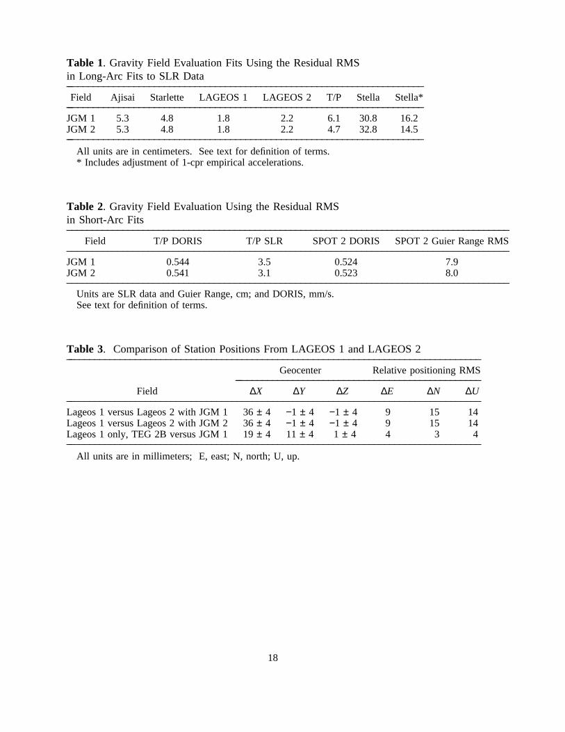
Table 1. Gravity Field Evaluation Fits Using the Residual RMSin Long-Arc Fits to SLR Data_ ______________________________________________________________________Field Ajisai Starlette LAGEOS 1 LAGEOS 2 T/P Stella Stella*_ ______________________________________________________________________

JGM 1 5.3 4.8 1.8 2.2 6.1 30.8 16.2JGM 2 5.3 4.8 1.8 2.2 4.7 32.8 14.5_ ______________________________________________________________________

All units are in centimeters. See text for definition of terms.* Includes adjustment of 1-cpr empirical accelerations.

Table 2. Gravity Field Evaluation Using the Residual RMSin Short-Arc Fits_______________________________________________________________________________________

Field T/P DORIS T/P SLR SPOT 2 DORIS SPOT 2 Guier Range RMS_______________________________________________________________________________________JGM 1 0.544 3.5 0.524 7.9JGM 2 0.541 3.1 0.523 8.0_______________________________________________________________________________________

Units are SLR data and Guier Range, cm; and DORIS, mm/s.See text for definition of terms.

Table 3. Comparison of Station Positions From LAGEOS 1 and LAGEOS 2_ _________________________________________________________________________________Geocenter Relative positioning RMS_ ________________________________________________

Field ∆X ∆Y ∆Z ∆E ∆N ∆U_ _________________________________________________________________________________Lageos 1 versus Lageos 2 with JGM 1 36 ± 4 −1 ± 4 −1 ± 4 9 15 14Lageos 1 versus Lageos 2 with JGM 2 36 ± 4 −1 ± 4 −1 ± 4 9 15 14Lageos 1 only, TEG 2B versus JGM 1 19 ± 4 11 ± 4 1 ± 4 4 3 4_ _________________________________________________________________________________

All units are in millimeters; E, east; N, north; U, up.

18

Table 4. Comparison of Station Positions forSPOT 2 versus SLR/VLBI_ _____________________________________________________________

Relative Positioning RMS_ ________________________________________Field ∆E ∆N ∆U_ _____________________________________________________________

JGM 1 72 36 40JGM 2 53 35 41JGM 2* 33 22 25_ _____________________________________________________________

All units are in millimeters. See text for definition of terms..*Included estimating selected gravity coefficients.

Table 5. Effective Data Standard Deviations in JGM 3 Solution_ _____________________________________________________________

Data Set Effective Standard Deviation_ _____________________________________________________________

T/P (DORIS) 6 mm/sT/P (GPS) 13 cmLAGEOS 2 (SLR) 30 cmLAGEOS 1 (SLR) 30 cmStella (SLR) 30 cmSPOT 2 (DORIS) 6 mm/s_ _____________________________________________________________

See text for definition of terms..

Table 6. Gravity Field Evaluation Fits Using the Residual RMS in Long-Arc Fits_ _________________________________________________________________________________________Field Ajisai Starlette LAGEOS 1 LAGEOS 2 T/P (SLR) T/P (DORIS) Stella Stella*_ _________________________________________________________________________________________

JGM 1 5.3 4.8 1.8 2.2 6.1 0.60 30.8 16.2JGM 2 5.3 4.8 1.8 2.2 4.7 0.54 32.8 14.5JGM 3A 5.1 4.8 1.7 1.9 4.0 0.53 7.0 4.2JGM 3B 5.0 4.8 1.7 1.9 4.2 0.53 7.3 4.6JGM 3C 5.2 4.8 1.7 1.9 3.9 0.53 10.9 8.5JGM 3 5.0 4.8 1.7 1.9 3.9 0.53 6.7 4.1_ _________________________________________________________________________________________

All units are centimeters or millimeters per second.* Include adjustment of 1-cpr acceleration parameters.

19

Table 7. Gravity Field Evaluation Using the Residual RMS in Short-Arc Fits_ ___________________________________________________________________________________Field T/P DORIS T/P SLR SPOT 2 DORIS SPOT 2 Guier Range RMS_ ___________________________________________________________________________________

JGM 1 0.544 3.5 0.524 7.9JGM 2 0.541 3.1 0.523 8.0JGM 3A 0.539 3.0 0.516 7.4JGM 3B 0.538 3.0 0.516 7.4JGM 3 0.539 3.0 0.516 7.4_ ___________________________________________________________________________________

Units are SLR data and Guier Range, cm; DORIS, mm/s.

Table 8. SLR/DORIS Orbit Comparisons With GPS Reduced DynamicTrajectories for TOPEX/Poseidon_ _______________________________________________________________________________

Radial RMS_ __________________________________________________________Cycle JGM 2 JGM 3 JGM 3A JGM 3B Z shift_ _______________________________________________________________________________14 30 21 23 24 −1615* 31 23 23 27 −2617* 30 26 25 28 −2318 27 24 24 24 −2319* 29 26 28 26 −3220 30 22 24 24 −3021 27 21 23 22 −2732 29 20 23 22 −22

Average 29 23 24 25 -25_ _______________________________________________________________________________All units are millimeters.*Indicates GPS tracking from this cycle used in gravity solution.

Table 9. Comparison of Station Positions for LAGEOS 1versus LAGEOS 2_ ___________________________________________________________________________

Geocenter Relative positioning RMS_ ________________________________________________________________Field ∆X ∆Y ∆Z ∆E ∆N ∆U_ ___________________________________________________________________________

JGM 2 36 ± 4 −1 ± 4 −1 ± 4 9 15 14JGM 3 4 ± 4 3 ± 4 6 ± 4 6 8 9_ ___________________________________________________________________________

All units are millimeters.

20

Table 10. Comparison of Station Positions for SPOT 2versus SLR/VLBI_ __________________________________________________________

Relative Positioning RMS_ _______________________________________Field ∆E ∆N ∆U_ __________________________________________________________

JGM 2 53 35 41JGM 3 33 22 25_ __________________________________________________________

All units are millimeters.

Table 11. Geoid Undulation Differences_ __________________________________________________Fields Total RMS Land RMS Ocean RMS_ __________________________________________________

JGM 2 JGM 3 20 30 14JGM 2 JGM 3A 17 25 12JGM 3 JGM 3A 9 13 6_ __________________________________________________

All units are centimeters.

Table 12. Three-Year Mean SST Derived From T/PCompared With Levitus Topography_ __________________________________________________

Geoid RMS of Difference_ __________________________________________________OSU91A 18JGM 2 16JGM 3 15_ __________________________________________________

All units are centimeters.

21

Table 13. Geoid Comparison to GPS/Leveling_ _____________________________________________________Field Europe Canada Australia United States_ _____________________________________________________

OSU91A 33 31 35 21JGM 2 38 28 27 19JGM 3A 47 29 27 20JGM 3 47 28 26 19_ _____________________________________________________

All units are centimeters.

Table 14. Predicted Radial Orbit Errors Due to GravityModeling Errors_ __________________________________________________

Satellite JGM 1 JGM 2 JGM 3_ __________________________________________________TOPEX/Poseidon 3.4 2.2 0.9Geosat 7.4 6.7 5.1ERS 1/ERS 2 7.8 7.2 3.7_ __________________________________________________

All units are centimeters.

22