Embed Size (px)
Citation preview

INTERNATIONAL JOURNAL FOR NUMERICAL METHODS IN ENGINEERINGInt. J. Numer. Meth. Engng 2008; 75:43–57Published online 16 November 2007 in Wiley InterScience (www.interscience.wiley.com). DOI: 10.1002/nme.2244
The iterated sinh transformation
David Elliott1 and Peter R. Johnston2,∗,†
1School of Mathematics and Physics, University of Tasmania, Private Bag 37, Hobart, Tasmania 7001, Australia2School of Biomolecular and Physical Sciences, Griffith University, Nathan, Qld. 4111, Australia
SUMMARY
A sinh transformation has recently been proposed to improve the numerical accuracy of evaluating nearlysingular integrals using Gauss–Legendre quadrature. It was shown that the transformation could improvethe accuracy of evaluating such integrals, which arise in the boundary element method, by several ordersof magnitude. Here, this transformation is extended in an iterative fashion to allow the accurate evaluationof similar types of integrals that have more spiked integrands.
Results show that one iteration of this sinh transformation is preferred for nearly weakly singularintegrals, whereas two iterations lead to several orders of magnitude improvement in the evaluation ofnearly strongly singular integrals. The same observation applies when considering integrals of derivativesof the two-dimensional boundary element kernel. However, for these integrals, more iterations are requiredas the distance from the source point to the boundary element decreases. Copyright q 2007 John Wiley& Sons, Ltd.
Received 23 May 2007; Revised 13 September 2007; Accepted 10 October 2007
KEY WORDS: non-linear co-ordinate transformation; boundary element method; nearly singular integrals;numerical integration; sinh function
1. INTRODUCTION
Implementation of the boundary element method requires the accurate numerical evaluation ofintegrals of the form
I =∫ 1
−1g(x) f ((x−a0)
2+b20)dx (1)
where it is assumed that −1<a0<1 and 0<b0�1. The function f is assumed to have somesingularity (i.e. pole or branch point) when its argument is zero, that is, f has singularities atpoints z0 and z̄0 where z0=a0+ ib0. Although the integral I is not singular, since we are assuming
∗Correspondence to: Peter R. Johnston, School of Biomolecular and Physical Sciences, Griffith University, Nathan,Qld. 4111, Australia.
†E-mail: [email protected]
Copyright q 2007 John Wiley & Sons, Ltd.

44 D. ELLIOTT AND P. R. JOHNSTON
that 0<b0�1, it is said to be a ‘nearly singular’ integral. The function g is assumed to be ‘wellbehaved’. Here, three particular forms of the function f will be considered, say
f1(r)= lnr, f2(r)= 1
r, f3(r)= 1
r�(2)
where r2=(x−a0)2+b20 and �>0 is not necessarily an integer.Numerical evaluation of integrals of the above forms has received considerable attention over
many years [1–7]. These studies are all based on Gauss–Legendre quadrature, but either usea polynomial transformation of the Gauss–Legendre integration points or split the interval ofintegration at the ‘nearly singular point’, a0, and apply transformations in each subinterval.
Recently a transformation, based on the sinh function, was introduced to evaluate nearly singularintegrals [8]. One advantage of this new transformation is that it automatically incorporates theposition of the nearly singular point a0 into the transformation as well as the distance b0 fromthe source point to the element. It was also demonstrated that the sinh transformation provided asignificant improvement over the untransformed use of Gauss–Legendre quadrature and could beapplied to a wide variety of problems.
It was also mentioned in [8] that the sinh transformation performed better on ‘nearly weaklysingular integrals’ than it did with ‘nearly strongly singular integrals’. In the context of thispaper, a ‘nearly weakly/strongly singular integral’ is defined as an integral that would in fact beweakly/strongly singular if the source point was on the element over which the integration wasbeing performed. These integrals are characterized by integrands that are continuous over the rangeof integration, but which exhibit a high narrow spike around the nearly singular point a0.
With the above considerations in mind, this paper introduces an iterated sinh transformation,which is applicable to nearly strongly singular integrals. It is shown that the iterated sinh transfor-mation can further reduce relative errors in the numerical evaluation of nearly strongly singularintegrals by several orders of magnitude.
In the following section the iterated sinh transformation is introduced and several of its propertiesare discussed. Section 3 then considers several examples where zero, one and two iterations ofthe sinh transformation are used, as well as two existing transformations, and compares theirrelative errors. Finally, Section 4 makes some recommendations as to the use of the iterated sinhtransformation.
2. THE ITERATED SINH TRANSFORMATION
For the integral I of (1), the sinh transformation has been defined previously [8] asx=a0+b0 sinh(�0u−�0) (3)
It then follows that
dx=b0�0 cosh(�0u−�0)du (4)
and
(x−a0)2+b20 =b20 cosh
2(�0u−�0) (5)
Copyright q 2007 John Wiley & Sons, Ltd. Int. J. Numer. Meth. Engng 2008; 75:43–57DOI: 10.1002/nme

THE ITERATED SINH TRANSFORMATION 45
Upon choosing
�0= 1
2
{arcsinh
(1+a0b0
)+arcsinh
(1−a0b0
)}(6)
and
�0= 1
2
{arcsinh
(1+a0b0
)−arcsinh
(1−a0b0
)}(7)
it turns out that −1�x�1 maps into −1�u�1 so that, from (1),
I =b0�0
∫ 1
−1g(x(u))cosh(�0u−�0) f (b
20 cosh
2(�0u−�0))du (8)
For appropriate forms of the function f , the integrand will have singularities where
cosh(�0u−�0)=0 (9)
In the complex plane, there are an infinite number of solutions to this equation, but the nearestsingularities to the interval (−1,1) are at z1 and z̄1, say, where
z1 :=a1+ ib1 (10)
with
a1= �0�0
and b1= �
2�0(11)
It has been shown [9, Theorem 3.4] that the points z1 and z̄1 are ‘further away’ from the interval(−1,1) than are the original points z0 and z̄0 so that applying the same n-point Gauss–Legendrequadrature rule is likely to lead to smaller truncation errors than for the original integral.
It would therefore appear reasonable to apply this approach again and define an iterated sinhtransformation by letting
u=a1+b1 sinh(�1v−�1) (12)
where
�1= 1
2
{arcsinh
(1+a1b1
)+arcsinh
(1−a1b1
)}(13)
and
�1= 1
2
{arcsinh
(1+a1b1
)−arcsinh
(1−a1b1
)}(14)
The Jacobian of this transformation is now
du=b1�1 cosh(�1v−�1)dv (15)
Copyright q 2007 John Wiley & Sons, Ltd. Int. J. Numer. Meth. Engng 2008; 75:43–57DOI: 10.1002/nme

46 D. ELLIOTT AND P. R. JOHNSTON
-1
-0.8
-0.6
-0.4
-0.2
0
0.2
0.4
0.6
0.8
1
-1 -0.8 -0.6 -0.4 -0.2 0 0.2 0.4 0.6 0.8 1
Tran
sfor
med
x-c
oord
inat
e
Original x-coordinate
Iteration 0Iteration 1Iteration 2
Figure 1. Effects of zero, one and two iterations of the sinh transformation on the Gauss–Legendrequadrature points with a0=0.25 and b0=0.01 for 20 integration points. The two horizontal lines indicate
how the integration points are clustered around the nearly singular point at x=0.25.
and, from (8), the integral I becomes
I = �b0�12
∫ 1
−1g(x(u(v)))cosh(�1v−�1)cosh(�sinh(�1v−�1)/2)
× f (b20 cosh2(�sinh(�1v−�1)/2))dv (16)
since, from (11), �0a1−�0=0 and �0b1=�/2. The singularities of appropriate forms of thefunction f will now be even further removed from the interval of integration (−1,1) than before,so that n-point Gauss–Legendre quadrature should be even better.
The idea behind a transformation technique for evaluating nearly singular integrals is to shiftthe integration points to regions where the integrand exhibits a spike. As discussed previously in[8], the sinh transformation automatically accounts for the nearly singular point and its distancefrom the interval of integration. Figure 1 shows the effect that the transformations (3) and (12)have on the original Gauss–Legendre nodes points (Iteration 0) with a0=0.25 and b0=0.01, for20 integration points. Such a transformation would be applicable when the function f has a nearsingularity at x=0.25. Note that the original Gauss–Legendre quadrature points are clusteredtowards the ends of the interval of integration and there are few near the point of interest atx=0.25. It can be seen that the first iteration (Iteration 1) clusters the integration points around thenearly singular point. A second iteration of the transformation clusters the integration points evenmore strongly around x=0.25. Hence, for an integral that is nearly strongly singular, it would beexpected that the second iteration of the sinh transformation would more accurately evaluate theintegral but, as we shall see in the following section, this is not always the case.
Copyright q 2007 John Wiley & Sons, Ltd. Int. J. Numer. Meth. Engng 2008; 75:43–57DOI: 10.1002/nme

THE ITERATED SINH TRANSFORMATION 47
3. RESULTS AND DISCUSSION
To demonstrate the accuracy of the above transformations, several prototype integrals will beevaluated. The numerical values obtained will be compared with exact values in terms of therelative error defined by
Relative error= |Inumerical− Iexact||Iexact| (17)
where Inumerical is the value obtained for the integral using the indicated numerical method andIexact is the exact value of the integral. The integrals in Sections 3.1 and 3.2 can be obtainedanalytically using the tables of integrals [10, 11]. Their values are given in Table I. ‘Exact’ valuesfor the examples in Section 3.3 were obtained numerically using the quadl routine in MATLABto a tolerance of 10−15.
Results are also compared with the transformation methods of Telles and Oliveira [2] and of Maand Kamiya [7]. Comparisons are made with the Telles and Oliveira transformation only for theintegrals with lnr , r−1, r−2 and r−3 type kernels, as these were the integrals for which the originaltransformation was designed. Also, comparisons are made only for b0=0.1 and b0=0.01 sinceparameter values used in the transformation are available only for these distances. In comparisonwith the transformation of Ma and Kamiya, it should be noted that this transformation splitsthe interval of integration into two subintervals at the point a0; hence in order to achieve a faircomparison in terms of computational load, only half the indicated number of nodes are used ineach subinterval, giving the same total number of function evaluations for all methods. However,in Table II, when 15 and 25 integration points are used for the Telles and Oliveira and iteratedsinh transformations, 8 and 13 integration points, respectively, were used on each subinterval inthe Ma and Kamiya transformation so that in both cases there is an additional function evaluation.
3.1. Nearly weakly singular integrals
Consider the numerical evaluation of the integrals
I1=∫ 1
−1(1−x2) ln
((x− 1
4
)2
+b20
)dx (18)
and
I2=∫ 1
−1
1−x2√(x− 1
4 )2+b20
dx (19)
The integral I1 is nearly weakly singular in the sense of the definition given in Section 1. However,although the integral I2 with b0=0 is actually a Hadamard finite-part integral, in this context itwill be considered to be nearly weakly singular in the sense that transformation (3) removes thenearly singular, or spiked, behaviour of the integrand.
The integral I1 represents an integral over a straight boundary element with the logarithmickernel and a basis function g(x)=1−x2. The nearly singular point is at x= 1
4 and the distancefrom the source point to the element is given by b0. The integral I2 also represents integration over
Copyright q 2007 John Wiley & Sons, Ltd. Int. J. Numer. Meth. Engng 2008; 75:43–57DOI: 10.1002/nme

48 D. ELLIOTT AND P. R. JOHNSTON
TableI.Exact
values
oftheintegralsI j,forj=
1,..
.,5,
fordifferentdistancesfrom
thesource
pointto
theelem
ent,b 0.
b 0I 1
I 2I 3
I 4I 5
0.1
−1.377
2802
1397
9331
×100
4.77
2986
5708
0824
3×1
002.60
0687
7822
9154
1×1
011.82
6962
4641
6369
3×1
021.45
8421
6641
2563
4×1
03
0.01
−1.624
8246
9087
8743
×100
9.06
1860
1394
1195
2×1
002.90
8109
8831
3288
9×1
021.87
4060
1134
8466
8×1
041.47
2465
9936
8396
5×1
06
0.00
1−1
.651
1475
6418
5811
×100
1.33
7869
4750
0417
2×1
012.94
1501
6656
2793
1×1
031.87
4985
9960
6591
3×1
061.47
2619
9870
9092
5×1
09
0.00
01−1
.653
7964
3046
2390
×100
1.76
9603
4395
4842
8×1
012.94
4868
6854
3602
9×1
041.87
4999
8139
0896
7×1
081.47
2621
5406
6376
9×1
012
0.00
001
−1.654
0614
8380
7876
×100
2.20
1338
1348
0133
2×1
012.94
5205
6671
8270
8×1
051.87
4999
9976
7857
3×1
0101.47
2621
5562
1313
8×1
015
0.00
0001
−1.654
0879
9081
0535
×100
2.63
3072
8396
1808
5×1
012.94
5239
3681
5638
5×1
061.87
4999
9999
7218
1×1
0121.47
2621
5563
6864
8×1
018
Copyright q 2007 John Wiley & Sons, Ltd. Int. J. Numer. Meth. Engng 2008; 75:43–57DOI: 10.1002/nme
THE ITERATED SINH TRANSFORMATION 49
Table II. Relative errors for the evaluation of the integral I1 using the Telles and Oliveira self-adaptivetransformation [2], the Ma and Kamiya transformation [7] and zero, one and two iterations of the sinhtransformation. The integral is evaluated at different distances from the source point to the element, b0,
and for different numbers of integration points, n.
Telles and Ma andb0 n Oliveira [2] Kamiya [7] Iteration 0 Iteration 1 Iteration 2
0.1 10 9.7541×10⁻⁶ 3.2956×10⁻³ 1.0901×10⁻² 3.2615×10⁻⁸ 1.8485×10⁻⁴
15 4.5780×10⁻⁷ 2.6141×10⁻⁶ 8.0194×10⁻⁴ 8.8914×10⁻¹⁰ 5.2305×10⁻⁸
20 2.7726×10⁻¹⁰ 8.2077×10⁻⁸ 1.0714×10⁻³ 5.0884×10⁻¹² 3.6081×10⁻¹²
25 1.9357×10⁻¹¹ 1.3131×10⁻⁹ 4.2946×10⁻⁴ 1.7089×10⁻¹⁴ 1.6122×10⁻¹⁶
30 9.0847×10⁻¹³ 7.3463×10⁻¹¹ 1.1551×10⁻⁴ 1.6122×10⁻¹⁶ 3.2244×10⁻¹⁶
0.01 10 7.2515×10⁻⁴ 1.6406×10⁻² 7.4987×10⁻² 5.0077×10⁻⁵ 1.0180×10⁻²
15 8.7817×10⁻⁴ 7.0521×10⁻⁵ 2.0494×10⁻² 4.0451×10⁻⁸ 1.0266×10⁻⁴
20 2.7006×10⁻⁴ 7.7545×10⁻⁷ 1.9754×10⁻² 2.2183×10⁻⁹ 2.3364×10⁻⁷
25 2.0660×10⁻⁶ 5.0644×10⁻⁹ 5.1374×10⁻² 1.7689×10⁻¹⁰ 2.0456×10⁻¹⁰
30 3.9710×10⁻⁵ 2.1282×10⁻⁹ 3.8063×10⁻² 8.8656×10⁻¹² 8.8828×10⁻¹⁴
0.001 10 3.4543×10⁻² 8.8599×10⁻² 1.1121×10⁻³ 3.3658×10⁻²
15 7.2079×10⁻⁴ 3.3347×10⁻² 5.5480×10⁻⁷ 2.6674×10⁻³
20 1.3380×10⁻⁵ 1.1849×10⁻² 1.2093×10⁻⁸ 3.9696×10⁻⁵
25 1.3571×10⁻⁸ 7.8515×10⁻² 4.3573×10⁻¹⁰ 2.2625×10⁻⁷
30 5.0562×10⁻¹⁰ 6.9897×10⁻² 1.6341×10⁻¹⁰ 6.3635×10⁻¹⁰
0.0001 10 4.3489×10⁻² 9.0047×10⁻² 5.6818×10⁻³ 2.0285×10⁻²
15 3.0377×10⁻³ 3.4868×10⁻² 6.8412×10⁻⁶ 1.3398×10⁻²
20 1.2173×10⁻⁴ 1.0319×10⁻² 3.0321×10⁻⁸ 6.8031×10⁻⁴
25 2.6266×10⁻⁷ 7.7676×10⁻² 2.2324×10⁻⁹ 1.3165×10⁻⁵
30 6.1648×10⁻¹⁰ 6.9458×10⁻² 2.4556×10⁻¹¹ 1.2695×10⁻⁷
0.00001 10 3.4423×10⁻² 9.0196×10⁻² 1.4792×10⁻² 5.6625×10⁻²
15 7.8961×10⁻³ 3.5022×10⁻² 6.8335×10⁻⁵ 3.0057×10⁻²
20 5.5849×10⁻⁴ 1.0159×10⁻² 3.8002×10⁻⁹ 3.7642×10⁻³
25 2.8437×10⁻⁶ 7.7512×10⁻² 2.7269×10⁻⁹ 1.7440×10⁻⁴
30 4.0656×10⁻⁸ 6.9302×10⁻² 3.2817×10⁻¹⁰ 4.0813×10⁻⁶
0.000001 10 5.2536×10⁻³ 9.0207×10⁻² 2.6561×10⁻² 1.7803×10⁻¹
15 1.5154×10⁻² 3.5037×10⁻² 3.4808×10⁻⁴ 4.1221×10⁻²
20 1.6824×10⁻³ 1.0142×10⁻² 3.9536×10⁻⁷ 1.1036×10⁻²
25 1.7525×10⁻⁵ 7.7499×10⁻² 1.4228×10⁻⁹ 9.8925×10⁻⁴
30 4.0501×10⁻⁷ 6.9283×10⁻² 2.5204×10⁻¹⁰ 4.5316×10⁻⁵
a straight element, this time with a 1/r type integrand and the same basis function. This integralhas been considered previously in [8].
Table II shows the relative errors for numerical evaluation of the integral I1 with the nearlysingular point at x= 1
4 for various values of b0 and various numbers of integration points, n.
Copyright q 2007 John Wiley & Sons, Ltd. Int. J. Numer. Meth. Engng 2008; 75:43–57DOI: 10.1002/nme
50 D. ELLIOTT AND P. R. JOHNSTON
It can be seen from the table that in all cases one iteration of the transformation leads to aconsiderable improvement in the accuracy of the numerical calculation over using straightforwardGauss–Legendre quadrature (no iterations). Also, the transformations of Telles and Oliveira andMa and Kamiya are an improvement over standard Gauss–Legendre quadrature but are not asaccurate as one iteration of the sinh transformation. For the largest b0 value considered, the Tellesand Oliveira transformation is more accurate than the Ma and Kamiya transformation.
Note that in most cases a second iteration of the transformation yields less accurate results,especially at small b0 values. One possible explanation is that the second iteration unnecessarilypushes too many integration points towards the nearly singular point, resulting in insufficientevaluation of the integrand away from this point. From another point of view, one iteration of thesinh transformation results in the integral
I1=2b0�0
∫ 1
−1(1−x2(u))cosh(�0u−�0) ln(b0 cosh(�0u−�0))du (20)
where �0 and �0 are given by (6) and (7), respectively, with a0= 14 . The integral now contains an
integrand that has had its spike removed. In this case, one iteration of the sinh transformation issufficient.
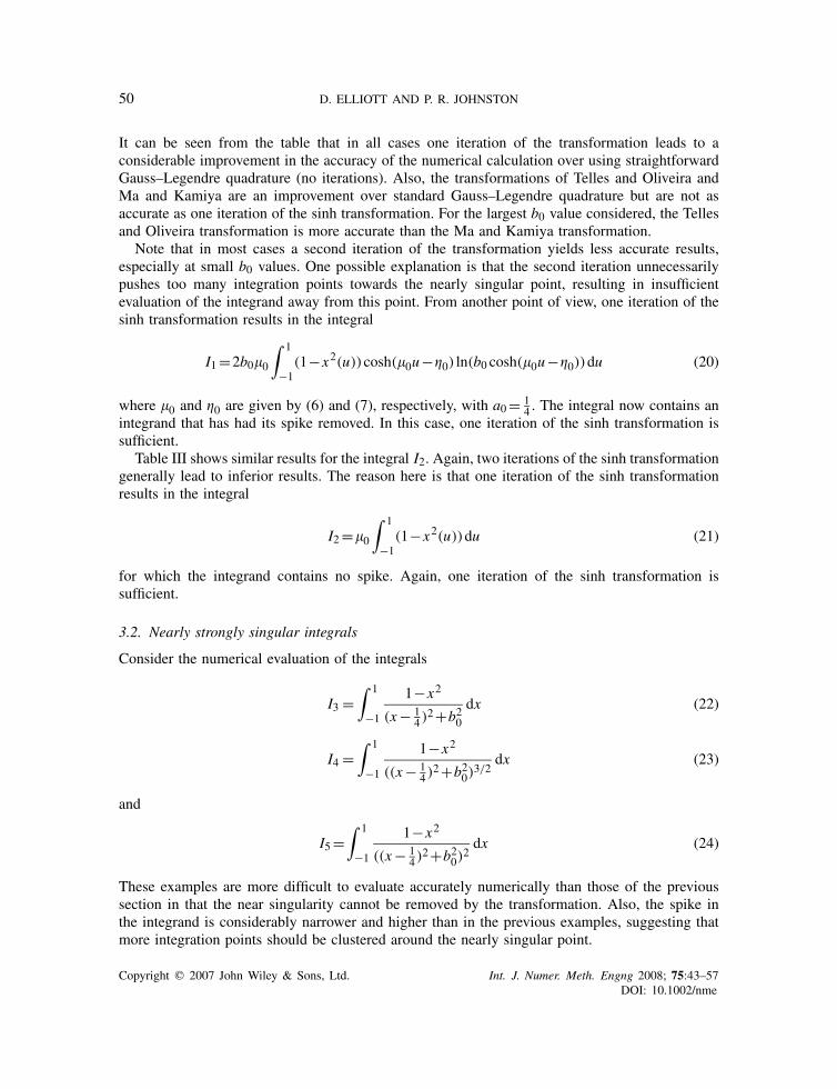
Table III shows similar results for the integral I2. Again, two iterations of the sinh transformationgenerally lead to inferior results. The reason here is that one iteration of the sinh transformationresults in the integral
I2=�0
∫ 1
−1(1−x2(u))du (21)
for which the integrand contains no spike. Again, one iteration of the sinh transformation issufficient.
3.2. Nearly strongly singular integrals
Consider the numerical evaluation of the integrals
I3 =∫ 1
−1
1−x2
(x− 14 )
2+b20dx (22)
I4 =∫ 1
−1
1−x2
((x− 14 )
2+b20)3/2
dx (23)
and
I5=∫ 1
−1
1−x2
((x− 14 )
2+b20)2dx (24)
These examples are more difficult to evaluate accurately numerically than those of the previoussection in that the near singularity cannot be removed by the transformation. Also, the spike inthe integrand is considerably narrower and higher than in the previous examples, suggesting thatmore integration points should be clustered around the nearly singular point.
Copyright q 2007 John Wiley & Sons, Ltd. Int. J. Numer. Meth. Engng 2008; 75:43–57DOI: 10.1002/nme
THE ITERATED SINH TRANSFORMATION 51
Table III. Relative errors for the evaluation of the integral I2 using the Telles and Oliveira self-adaptivetransformation [2], the Ma and Kamiya transformation [7] and zero, one and two iterations of the sinh
transformation. The format is the same as that for Table II.
Telles and Ma andb0 n Oliveira [2] Kamiya [7] Iteration 0 Iteration 1 Iteration 2
0.1 10 6.1011×10⁻⁵ 6.1774×10⁻⁴ 3.7637×10⁻² 1.8346×10⁻¹¹ 2.2359×10⁻⁶
15 6.8701×10⁻⁷ 8.5247×10⁻⁶ 2.3361×10⁻³ 3.7218×10⁻¹⁶ 8.9212×10⁻¹¹
20 7.5213×10⁻⁹ 4.7085×10⁻⁷ 4.7742×10⁻³ 1.8608×10⁻¹⁶ 1.1165×10⁻¹⁵
25 1.2932×10⁻¹⁰ 4.1281×10⁻⁹ 2.1978×10⁻³ 0.0000×10+00 1.8608×10⁻¹⁶
30 9.1405×10⁻¹³ 3.0609×10⁻¹¹ 6.5785×10⁻⁴ 1.8608×10⁻¹⁶ 1.8608×10⁻¹⁶
0.01 10 4.5881×10⁻³ 2.2767×10⁻³ 3.8395×10⁻¹ 3.8039×10⁻⁸ 2.9066×10⁻⁴
15 2.9275×10⁻³ 2.9661×10⁻⁵ 2.0792×10⁻¹ 3.5284×10⁻¹⁵ 3.6078×10⁻⁷
20 3.3319×10⁻⁴ 1.5771×10⁻⁵ 6.1187×10⁻² 1.9603×10⁻¹⁶ 1.4686×10⁻¹⁰
25 5.7075×10⁻⁶ 4.7182×10⁻⁷ 5.1925×10⁻¹ 3.9205×10⁻¹⁶ 2.7640×10⁻¹⁴
30 6.6224×10⁻⁶ 8.2593×10⁻⁸ 4.3270×10⁻¹ 1.9603×10⁻¹⁶ 3.9205×10⁻¹⁶
0.001 10 1.2572×10⁻³ 5.8154×10⁻¹ 1.8163×10⁻⁶ 2.2667×10⁻³
15 1.2005×10⁻⁵ 4.5735×10⁻¹ 5.0103×10⁻¹² 1.7418×10⁻⁵
20 6.6160×10⁻⁵ 2.3937×10⁻¹ 1.3278×10⁻¹⁵ 4.5133×10⁻⁸
25 5.3701×10⁻⁶ 6.6515×10⁻¹ 1.3278×10⁻¹⁶ 5.3712×10⁻¹¹
30 1.0856×10⁻⁶ 8.0725×10⁻¹ 6.6388×10⁻¹⁶ 3.5850×10⁻¹⁴
0.0001 10 1.0352×10⁻² 6.8360×10⁻¹ 1.8068×10⁻⁵ 6.3398×10⁻³
15 7.7421×10⁻⁴ 5.8968×10⁻¹ 4.6118×10⁻¹⁰ 1.5597×10⁻⁴
20 1.9258×10⁻⁴ 4.2458×10⁻¹ 9.2348×10⁻¹⁵ 1.3522×10⁻⁶
25 1.8807×10⁻⁵ 2.7226×10⁻¹ 4.4168×10⁻¹⁵ 5.4925×10⁻⁹
30 5.2761×10⁻⁶ 3.9159×10⁻¹ 7.4282×10⁻¹⁵ 1.2327×10⁻¹¹
0.00001 10 1.2214×10⁻² 7.4568×10⁻¹ 8.0392×10⁻⁵ 1.0995×10⁻²
15 3.5478×10⁻⁴ 6.7018×10⁻¹ 1.0336×10⁻⁸ 6.0799×10⁻⁴
20 2.2635×10⁻⁵ 5.3745×10⁻¹ 1.5025×10⁻¹³ 1.2472×10⁻⁵
25 4.8423×10⁻⁵ 2.2850×10⁻² 6.9399×10⁻¹⁴ 1.2325×10⁻⁷
30 1.2031×10⁻⁵ 1.1888×10⁻¹ 2.8405×10⁻¹⁴ 6.8290×10⁻¹⁰
0.000001 10 8.4724×10⁻³ 7.8737×10⁻¹ 2.2492×10⁻⁴ 1.4802×10⁻²
15 1.7007×10⁻³ 7.2425×10⁻¹ 9.8501×10⁻⁸ 1.4835×10⁻³
20 5.4050×10⁻⁴ 6.1328×10⁻¹ 2.9194×10⁻¹² 5.8035×10⁻⁵
25 9.2354×10⁻⁶ 1.4486×10⁻¹ 5.3591×10⁻¹³ 1.1300×10⁻⁶
30 2.2429×10⁻⁶ 6.4579×10⁻² 2.5582×10⁻¹³ 1.2571×10⁻⁸
Table IV shows the relative errors for the numerical evaluation of the integral I3 with the nearlysingular point at x= 1
4 and various values of b0. This table shows that while one iteration ofthe sinh transformation remarkably improves the numerical evaluation of the integral (by severalorders of magnitude in many cases), a second iteration improves the numerical evaluation again(also by several orders of magnitude). The improvement is often more dramatic at smaller values
Copyright q 2007 John Wiley & Sons, Ltd. Int. J. Numer. Meth. Engng 2008; 75:43–57DOI: 10.1002/nme

52 D. ELLIOTT AND P. R. JOHNSTON
Table IV. Relative errors for the evaluation of the integral I3 using the Telles and Oliveira self-adaptivetransformation [2], the Ma and Kamiya transformation [7] and zero, one and two iterations of the sinh
transformation. The format is the same as that for Table II.
Telles and Ma andb0 n Oliveira [2] Kamiya [7] Iteration 0 Iteration 1 Iteration 2
0.1 10 9.1284×10⁻⁴ 2.3659×10⁻³ 1.4086×10⁻¹ 3.3754×10⁻⁶ 4.1270×10⁻⁹
15 6.0822×10⁻⁶ 2.6471×10⁻⁵ 6.6559×10⁻³ 4.2570×10⁻⁷ 3.9451×10⁻¹³
20 1.5644×10⁻⁶ 6.8471×10⁻⁷ 2.2522×10⁻² 3.9566×10⁻⁹ 0.0000×10+00
25 7.8967×10⁻⁹ 2.7174×10⁻⁸ 1.1760×10⁻² 1.9286×10⁻¹¹ 4.0981×10⁻¹⁶
30 1.8558×10⁻⁹ 3.8993×10⁻⁹ 3.8824×10⁻³ 2.2404×10⁻¹⁴ 1.3661×10⁻¹⁶
0.01 10 1.2143×10⁻³ 1.5566×10⁻² 8.7050×10⁻¹ 4.6976×10⁻³ 8.6692×10⁻⁷
15 1.5905×10⁻² 9.7852×10⁻⁴ 6.8866×10⁻¹ 5.8798×10⁻⁵ 6.5672×10⁻¹⁰
20 4.0328×10⁻³ 8.0676×10⁻⁵ 1.1916×10⁻¹ 7.5193×10⁻⁶ 3.0414×10⁻¹³
25 1.6650×10⁻⁴ 8.0485×10⁻⁶ 1.8837×10+0 8.7249×10⁻⁷ 5.8639×10⁻¹⁶
30 3.0927×10⁻⁶ 1.1947×10⁻⁷ 1.7297×10+0 6.1325×10⁻⁸ 1.9546×10⁻¹⁶
0.001 10 4.4340×10⁻² 9.8708×10⁻¹ 4.0194×10⁻² 8.7829×10⁻⁶
15 4.0768×10⁻³ 9.6811×10⁻¹ 3.4693×10⁻³ 1.5891×10⁻⁸
20 6.1359×10⁻⁵ 8.9668×10⁻¹ 1.8263×10⁻⁴ 2.2940×10⁻¹¹
25 5.9407×10⁻⁶ 3.2903×10⁻³ 1.2371×10⁻⁵ 3.5094×10⁻¹⁴
30 1.6861×10⁻⁵ 4.1652×10⁻¹ 5.9330×10⁻⁶ 4.1741×10⁻¹⁵
0.0001 10 6.7915×10⁻² 9.9872×10⁻¹ 1.2006×10⁻¹ 3.0635×10⁻⁵
15 1.7393×10⁻³ 9.9682×10⁻¹ 2.0564×10⁻² 9.9393×10⁻⁸
20 2.0854×10⁻³ 9.8965×10⁻¹ 3.0042×10⁻³ 2.8017×10⁻¹⁰
25 2.0573×10⁻⁵ 8.9783×10⁻¹ 3.2494×10⁻⁴ 8.0360×10⁻¹³
30 6.0341×10⁻⁵ 8.5206×10⁻¹ 2.9834×10⁻⁶ 4.2002×10⁻¹⁵
0.00001 10 2.3184×10⁻² 9.9986×10⁻¹ 2.2969×10⁻¹ 7.2012×10⁻⁵
15 2.1627×10⁻² 9.9969×10⁻¹ 5.9347×10⁻² 3.5441×10⁻⁷
20 5.8159×10⁻³ 9.9898×10⁻¹ 1.3426×10⁻² 1.5373×10⁻⁹
25 8.3287×10⁻⁴ 9.8978×10⁻¹ 2.7432×10⁻³ 6.1096×10⁻¹²
30 2.8763×10⁻⁴ 9.8519×10⁻¹ 4.6221×10⁻⁴ 1.5574×10⁻¹³
0.000001 10 1.4089×10⁻¹ 9.9999×10⁻¹ 3.4904×10⁻¹ 1.4501×10⁻⁴
15 2.3148×10⁻² 9.9995×10⁻¹ 1.2101×10⁻¹ 9.3782×10⁻⁷
20 7.5537×10⁻³ 9.9988×10⁻¹ 3.5335×10⁻² 5.3646×10⁻⁹
25 1.7200×10⁻³ 9.9897×10⁻¹ 9.9618×10⁻³ 3.1284×10⁻¹¹
30 5.7267×10⁻⁴ 9.9853×10⁻¹ 2.5951×10⁻³ 1.6732×10⁻¹²
of b0. Also at small b0 values, the transformation of Ma and Kamiya is generally superior to oneiteration of the sinh transformation.
Similar results are shown in Tables V and VI for the numerical evaluation of the integrals I4and I5, respectively. In both cases, applications of one and two iterations of the sinh transfor-mation lead to similar levels of improvement to that shown for the numerical evaluation of theintegral I3.
Copyright q 2007 John Wiley & Sons, Ltd. Int. J. Numer. Meth. Engng 2008; 75:43–57DOI: 10.1002/nme
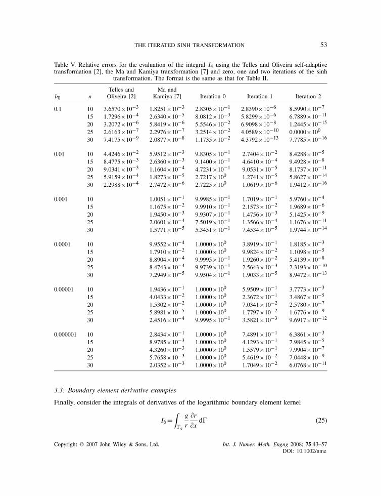
THE ITERATED SINH TRANSFORMATION 53
Table V. Relative errors for the evaluation of the integral I4 using the Telles and Oliveira self-adaptivetransformation [2], the Ma and Kamiya transformation [7] and zero, one and two iterations of the sinh
transformation. The format is the same as that for Table II.
Telles and Ma andb0 n Oliveira [2] Kamiya [7] Iteration 0 Iteration 1 Iteration 2
0.1 10 3.6570×10⁻³ 1.8251×10⁻³ 2.8305×10⁻¹ 2.8390×10⁻⁶ 8.5990×10⁻⁷
15 1.7296×10⁻⁴ 2.6340×10⁻⁵ 8.0812×10⁻³ 5.8299×10⁻⁶ 6.7889×10⁻¹¹
20 3.2072×10⁻⁶ 5.8419×10⁻⁶ 5.5546×10⁻² 6.9098×10⁻⁸ 1.2445×10⁻¹⁵
25 2.6163×10⁻⁷ 2.2976×10⁻⁷ 3.2514×10⁻² 4.0589×10⁻¹⁰ 0.0000×100
30 7.4175×10⁻⁹ 2.0877×10⁻⁸ 1.1735×10⁻² 4.3792×10⁻¹³ 7.7785×10⁻¹⁶
0.01 10 4.4246×10⁻² 5.9512×10⁻³ 9.8305×10⁻¹ 2.7404×10⁻² 8.4288×10⁻⁵
15 8.4775×10⁻³ 2.6360×10⁻³ 9.1400×10⁻¹ 4.6410×10⁻⁴ 9.4928×10⁻⁸
20 9.0341×10⁻³ 1.1604×10⁻⁴ 4.7231×10⁻¹ 9.0531×10⁻⁵ 8.1737×10⁻¹¹
25 5.9159×10⁻⁴ 1.8273×10⁻⁵ 2.7217×100 1.2741×10⁻⁵ 5.8627×10⁻¹⁴
30 2.2988×10⁻⁴ 2.7472×10⁻⁶ 2.7225×100 1.0619×10⁻⁶ 1.9412×10⁻¹⁶
0.001 10 1.0051×10⁻¹ 9.9985×10⁻¹ 1.7019×10⁻¹ 5.9760×10⁻⁴
15 1.1675×10⁻² 9.9910×10⁻¹ 2.1573×10⁻² 1.9689×10⁻⁶
20 1.9450×10⁻³ 9.9307×10⁻¹ 1.4756×10⁻³ 5.1425×10⁻⁹
25 2.0601×10⁻⁴ 7.5019×10⁻¹ 1.3566×10⁻⁴ 1.1676×10⁻¹¹
30 1.5771×10⁻⁵ 5.3451×10⁻¹ 7.4534×10⁻⁵ 1.9744×10⁻¹⁴
0.0001 10 9.9552×10⁻⁴ 1.0000×100 3.8919×10⁻¹ 1.8185×10⁻³
15 1.7910×10⁻² 1.0000×100 9.9824×10⁻² 1.1098×10⁻⁵
20 8.8904×10⁻⁴ 9.9995×10⁻¹ 1.9260×10⁻² 5.4139×10⁻⁸
25 8.4743×10⁻⁴ 9.9739×10⁻¹ 2.5643×10⁻³ 2.3193×10⁻¹⁰
30 7.2949×10⁻⁵ 9.9504×10⁻¹ 1.9033×10⁻⁵ 8.9472×10⁻¹³
0.00001 10 1.9436×10⁻¹ 1.0000×100 5.9509×10⁻¹ 3.7773×10⁻³
15 4.0433×10⁻² 1.0000×100 2.3672×10⁻¹ 3.4867×10⁻⁵
20 1.5302×10⁻² 1.0000×100 7.0341×10⁻² 2.5780×10⁻⁷
25 5.8981×10⁻⁵ 1.0000×100 1.7797×10⁻² 1.6776×10⁻⁹
30 2.4516×10⁻⁴ 9.9995×10⁻¹ 3.5821×10⁻³ 9.6917×10⁻¹²
0.000001 10 2.8434×10⁻¹ 1.0000×100 7.4891×10⁻¹ 6.3861×10⁻³
15 8.9785×10⁻³ 1.0000×100 4.1293×10⁻¹ 7.9845×10⁻⁵
20 4.3260×10⁻³ 1.0000×100 1.5579×10⁻¹ 7.9904×10⁻⁷
25 5.7658×10⁻³ 1.0000×100 5.4619×10⁻² 7.0448×10⁻⁹
30 2.0352×10⁻³ 1.0000×100 1.7049×10⁻² 6.0768×10⁻¹¹
3.3. Boundary element derivative examples
Finally, consider the integrals of derivatives of the logarithmic boundary element kernel
I6=∫
�e
g
r
�r�x
d� (25)
Copyright q 2007 John Wiley & Sons, Ltd. Int. J. Numer. Meth. Engng 2008; 75:43–57DOI: 10.1002/nme

54 D. ELLIOTT AND P. R. JOHNSTON
Table VI. Relative errors for the evaluation of the integral I5 using the Ma and Kamiya transformation [7]and zero, one and two iterations of the sinh transformation. The format is the same as that for Table II.
b0 n Ma and Kamiya [7] Iteration 0 Iteration 1 Iteration 2
0.1 10 3.3393×10⁻³ 4.2689×10⁻¹ 1.3534×10⁻⁴ 1.3009×10⁻⁵
15 2.1193×10⁻⁴ 2.4647×10⁻³ 3.5894×10⁻⁵ 1.9830×10⁻⁹
20 2.2729×10⁻⁵ 1.0012×10⁻¹ 5.3986×10⁻⁷ 3.3519×10⁻¹⁴
25 5.7890×10⁻⁷ 6.4980×10⁻² 3.8052×10⁻⁹ 4.6771×10⁻¹⁶
30 4.0351×10⁻⁸ 2.5427×10⁻² 3.4854×10⁻¹² 3.1181×10⁻¹⁶
0.01 10 2.8079×10⁻² 9.9799×10⁻¹ 7.1323×10⁻² 9.4067×10⁻⁴
15 2.2557×10⁻³ 9.7870×10⁻¹ 1.5706×10⁻³ 2.1828×10⁻⁶
20 7.4214×10⁻⁴ 7.2681×10⁻¹ 4.5570×10⁻⁴ 3.1804×10⁻⁹
25 1.6764×10⁻⁶ 3.0298×100 7.7516×10⁻⁵ 3.4008×10⁻¹²
30 9.7214×10⁻⁶ 3.2860×100 7.6328×10⁻⁶ 2.5300×10⁻¹⁵
0.001 10 9.3078×10⁻² 9.9999×10⁻¹ 3.3447×10⁻¹ 5.3456×10⁻³
15 1.1270×10⁻² 9.9999×10⁻¹ 5.8250×10⁻² 3.6574×10⁻⁵
20 4.8958×10⁻³ 9.9958×10⁻¹ 5.0624×10⁻³ 1.6288×10⁻⁷
25 5.8331×10⁻⁴ 9.4885×10⁻¹ 6.1383×10⁻⁴ 5.6285×10⁻¹⁰
30 6.9074×10⁻⁵ 8.7511×10⁻¹ 3.8666×10⁻⁴ 1.6310×10⁻¹²
0.0001 10 1.2071×10⁻¹ 9.9999×10⁻¹ 6.2146×10⁻¹ 1.3933×10⁻²
15 4.1020×10⁻² 9.9999×10⁻¹ 2.1796×10⁻¹ 1.7675×10⁻⁴
20 9.7563×10⁻³ 9.9999×10⁻¹ 5.3374×10⁻² 1.4724×10⁻⁶
25 2.1840×10⁻³ 9.9992×10⁻¹ 8.5575×10⁻³ 9.6162×10⁻⁹
30 5.4143×10⁻⁴ 9.9985×10⁻¹ 4.4257×10⁻⁵ 5.3450×10⁻¹¹
0.00001 10 2.7789×10⁻¹ 9.9999×10⁻¹ 8.1406×10⁻¹ 2.5823×10⁻²
15 2.1870×10⁻² 9.9999×10⁻¹ 4.4521×10⁻¹ 4.9425×10⁻⁴
20 1.2612×10⁻² 9.9999×10⁻¹ 1.6346×10⁻¹ 6.2366×10⁻⁶
25 3.5280×10⁻³ 9.9999×10⁻¹ 4.9615×10⁻² 6.1922×10⁻⁸
30 8.7575×10⁻⁴ 9.9999×10⁻¹ 1.1762×10⁻² 5.2512×10⁻¹⁰
0.000001 10 2.6287×10⁻¹ 9.9999×10⁻¹ 9.1633×10⁻¹ 3.9917×10⁻²
15 6.8564×10⁻² 9.9999×10⁻¹ 7.0072×10⁻¹ 1.0305×10⁻³
20 3.0842×10⁻² 9.9999×10⁻¹ 3.1372×10⁻¹ 1.7582×10⁻⁵
25 5.8948×10⁻³ 9.9999×10⁻¹ 1.3143×10⁻¹ 2.3645×10⁻⁷
30 2.1127×10⁻³ 9.9999×10⁻¹ 4.8158×10⁻² 2.7290×10⁻⁹
and
I7=∫
�e
g��x
(1
r
�r�x
)d� (26)
where �e is the arc of a unit circle subtending an angle of 10◦ and r2=(x−x0)2+(y− y0)2 with(x0, y0) being the coordinate of the source point and (x, y) the coordinates of general points alongthe element �e. The integrals are transformed so that they are mapped onto the interval [−1,1]
Copyright q 2007 John Wiley & Sons, Ltd. Int. J. Numer. Meth. Engng 2008; 75:43–57DOI: 10.1002/nme

THE ITERATED SINH TRANSFORMATION 55
1e-16
1e-14
1e-12
1e-10
1e-08
1e-06
0.0001
0.01
1
0.0001 0.001 0.01 0.1 1
Rel
ativ
e E
rror
Distance to Element (b)
Iteration 0 (40)Iteration 1 (40)Iteration 2 (40)
Ma and Kamiya (40)
Figure 2. Relative errors for the numerical evaluation of the integral I6 as a function of distance from thesource point to the element, b, using various numbers of iterations of the sinh transformation as well asthe transformation of Ma and Kamiya [7] with a=0.2. Here 40 Gauss–Legendre quadrature points wereused in each of the sinh transformation iterations and 20 Gauss–Legendre quadrature points were used in
each half of the Ma and Kamiya transformation.
in terms of some intrinsic coordinate � along the element. After the transformation, r becomes√(�−a)2+b2 where a is the position of the nearly singular point and b the distance to the element.
Using the quadratic basis function g(�)=1−�2, the integrals become (using the ideas describedin [8])
I6=∫ 1
−1
(1−�2)(�−a)
(�−a)2+b2
√4(cos
�
36−1)2
�2+sin2�
36d� (27)
and
I7=∫ 1
−1
(1−�2)(b2−(�−a)2)
((�−a)2+b2)2
√4(cos
�
36−1)2
�2+sin2�
36d� (28)
Accurate evaluation of these integrals requires a larger number of integration points (even withthe transformations) due to the oscillations present in the integrands.
Figure 2 shows the relative errors for the evaluation of the integral I6 using 40 integration pointsfor a=0.2 and various values of b. It can be seen that at the smallest values of b, two iterationsof the sinh transformation produce an order of magnitude improvement over one iteration. Atintermediate values of b, say 0.005�b�0.05, both one and two iterations give similar results;thus, in this region one iteration would be sufficient. For b�0.05, the sinh transformation is notrequired at all. This example indicates that more transformations should be taken as the value of bdecreases. For all but the largest values of b, both one and two iterations of the sinh transformationgive superior results compared with the transformation of Ma and Kamiya, which in turn is asignificant improvement over standard Gauss–Legendre quadrature.
Copyright q 2007 John Wiley & Sons, Ltd. Int. J. Numer. Meth. Engng 2008; 75:43–57DOI: 10.1002/nme
56 D. ELLIOTT AND P. R. JOHNSTON
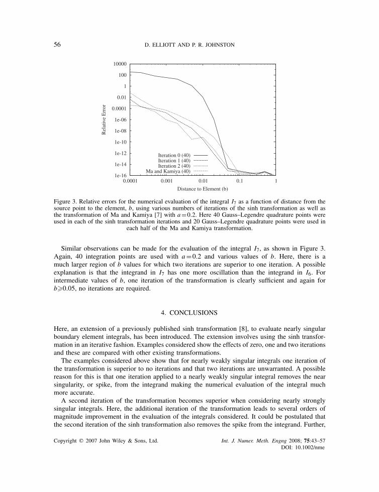
Figure 3. Relative errors for the numerical evaluation of the integral I7 as a function of distance from thesource point to the element, b, using various numbers of iterations of the sinh transformation as well asthe transformation of Ma and Kamiya [7] with a=0.2. Here 40 Gauss–Legendre quadrature points wereused in each of the sinh transformation iterations and 20 Gauss–Legendre quadrature points were used in
each half of the Ma and Kamiya transformation.
Similar observations can be made for the evaluation of the integral I7, as shown in Figure 3.Again, 40 integration points are used with a=0.2 and various values of b. Here, there is amuch larger region of b values for which two iterations are superior to one iteration. A possibleexplanation is that the integrand in I7 has one more oscillation than the integrand in I6. Forintermediate values of b, one iteration of the transformation is clearly sufficient and again forb�0.05, no iterations are required.
4. CONCLUSIONS
Here, an extension of a previously published sinh transformation [8], to evaluate nearly singularboundary element integrals, has been introduced. The extension involves using the sinh transfor-mation in an iterative fashion. Examples considered show the effects of zero, one and two iterationsand these are compared with other existing transformations.
The examples considered above show that for nearly weakly singular integrals one iteration ofthe transformation is superior to no iterations and that two iterations are unwarranted. A possiblereason for this is that one iteration applied to a nearly weakly singular integral removes the nearsingularity, or spike, from the integrand making the numerical evaluation of the integral muchmore accurate.
A second iteration of the transformation becomes superior when considering nearly stronglysingular integrals. Here, the additional iteration of the transformation leads to several orders ofmagnitude improvement in the evaluation of the integrals considered. It could be postulated thatthe second iteration of the sinh transformation also removes the spike from the integrand. Further,
Copyright q 2007 John Wiley & Sons, Ltd. Int. J. Numer. Meth. Engng 2008; 75:43–57DOI: 10.1002/nme

THE ITERATED SINH TRANSFORMATION 57
more strongly singular integrals could be evaluated more accurately with further iterations of thesinh transformation.
The final examples show that, firstly, more integration points are required when consideringderivatives of the logarithmic kernel in the boundary element method, which is due to the oscillatorynature of the integrand, and, secondly, that the number of iterations is more closely related to thedistance from the source point to the element b than the height of the spike caused by the nearsingularity. In other words, there is a range of values of b where no iteration is required, anotherwhere one iteration would suffice and others where more iterations are required.
Finally, it has been shown previously in [8] that splitting the interval of integration at the nearlysingular point can improve the accuracy of the numerical evaluation of the integral. This was notconsidered here, but it would be expected that a combination of splitting the integral and iterationsof the sinh transformation would further improve the accuracy.
REFERENCES
1. Telles JCF. A self-adaptive co-ordinate transformation for efficient numerical evaluation of general boundaryelement integrals. International Journal for Numerical Methods in Engineering 1987; 24:959–973.
2. Telles JCF, Oliveira RF. Third degree polynomial transformation for boundary element integrals: furtherimprovements. Engineering Analysis with Boundary Elements 1994; 13:135–141.
3. Johnston PR. Application of sigmoidal transformations to weakly singular and near-singular boundary elementintegrals. International Journal for Numerical Methods in Engineering 1999; 45(10):1333–1348.
4. Zhang D, Rizzo FJ, Rudolphi YJ. Stress intensity sensitivities via hypersingular boundary element integralequations. Computational Mechanics 1999; 23:389–396.
5. Sladek N, Sladek J, Tanaka M. Regularization of hypersingular and nearly singular integrals in the potentialtheory and elasticity. International Journal for Numerical Methods in Engineering 1993; 36:1609–1628.
6. Sladek V, Sladek J, Tanaka M. Numerical integration of logarithmic and nearly logarithmic singularity in BEMs.Applied Mathematical Modelling 2001; 25:901–922.
7. Ma H, Kamiya N. Distance transformation for the numerical evaluation of near singular boundary integrals withvarious kernels in boundary element method. Engineering Analysis with Boundary Elements 2002; 26:329–339.
8. Johnston PR, Elliott D. A sinh transformation for evaluating nearly singular boundary element integrals.International Journal for Numerical Methods in Engineering 2005; 62(4):564–578.
9. Elliott D, Johnston PR. Error analysis for a sinh transformation used in evaluating nearly singular boundaryelement integrals. Journal of Computational and Applied Mathematics 2007; 203(1):103–124.
10. Spiegel MR. Mathematical Handbook of Formulas and Tables (International edn). Schaum’s Outline Series.McGraw-Hill: New York, 1990.
11. Gradshteyn IS, Ryzhik IM. Table of Integrals, Series and Products (5th edn). Academic Press: Boston, 1994.
Copyright q 2007 John Wiley & Sons, Ltd. Int. J. Numer. Meth. Engng 2008; 75:43–57DOI: 10.1002/nme