J Stat Phys (2011) 145:549–590DOI 10.1007/s10955-011-0212-0

The Ising Susceptibility Scaling Function

Y. Chan · A.J. Guttmann · B.G. Nickel · J.H.H. Perk

Received: 10 March 2011 / Accepted: 25 April 2011 / Published online: 21 May 2011© Springer Science+Business Media, LLC 2011

Abstract We have dramatically extended the zero field susceptibility series at both highand low temperature of the Ising model on the triangular and honeycomb lattices, and usedthese data and newly available further terms for the square lattice to calculate a number ofterms in the scaling function expansion around both the ferromagnetic and, for the squareand honeycomb lattices, the antiferromagnetic critical point.

Keywords Ising model · Susceptibility · Triangular lattice · Honeycomb lattice · Seriesexpansion · Corrections to scaling

Cyril Domb was a pioneer in the application of series expansions to the study of criticalphenomena [1, 2]. He encouraged many colleagues to develop this approach and headeda group, the “Kings College group,” who applied his ideas to investigate the behaviour ofco-operative assemblies and percolation processes with considerable success. Domb’s un-selfish and generous attitude in urging people to follow up and develop the series approachwas an important factor in the subsequent evolution of research in these areas. It is there-fore with considerable pleasure that we dedicate this paper to Cyril Domb, on the occasionof his 90th birthday. In it we show just how powerful the series approach can be, as we

Y. Chan · A.J. GuttmannDepartment of Mathematics and Statistics, The University of Melbourne, Parkville, Victoria 3052,Australia

B.G. NickelDepartment of Physics, University of Guelph, Guelph, Ontario, Canada N1G 2W1

J.H.H. Perk (�)Department of Physics, Oklahoma State University, Stillwater, OK 74078-3072, USAe-mail: perk@okstate.edu

J.H.H. PerkDepartment of Theoretical Physics (RSPE) and Centre for Mathematics and its Applications (CMA),Australian National University, Canberra, ACT 2600, Australia

550 Y. Chan et al.

present an analysis based on hundreds, and in some cases thousands of terms in the expan-sion of the susceptibility of the two-dimensional Ising model. It would be fair to say that nomethod other than the series method provides anything remotely approaching this level ofinformation about the susceptibility.

1 Introduction

A decade ago a number of the current authors reported on a substantial extension of thesquare lattice Ising susceptibility series to some 300 terms [3, 4]. We found breakdown ofthe simple scaling picture that assumes the absence of irrelevant scaling fields. The firstbreakdown, which was identified with the breakdown of rotational symmetry of the squarelattice, occurred at O(τ 4), with τ to leading order proportional to the temperature deviationfrom critical, T −Tc. A second breakdown was identified at O(τ 6), ascribed to an additionalirrelevant variable. At the time it was foreshadowed that the corresponding calculation forthe triangular and honeycomb lattices would be necessary in order to distinguish betweenlattice effects and more fundamental breakdowns intrinsic to the model.

In this study we report on the derivation and analysis of triangular and honeycomb latticeseries to more than 300 terms, followed by a calculation of the corresponding scaling func-tions. Our numerical work is of sufficient accuracy that we can unambiguously identify thesame irrational constant, that appeared at O(τ 6) in the square lattice scaling function andwas ascribed to a second irrelevant variable, as a contribution to O(τ 6) in both triangularand honeycomb lattices. Furthermore, we find another irrational constant common to all lat-tices at O(τ 10) which can be ascribed to yet another (third) irrelevant variable. These resultsclearly indicate aspects of universality in the susceptibility beyond those found at leadingorder.

A limited selection of our results which are the basis for these remarks on universalityare given in the immediately following text while the very extensive complete listing can befound in the Appendices A–C. In subsequent sections we elaborate on the results below andgive details of how they were obtained. Specifically, in Sect. 2 we put our results in the con-text of scaling theory and speculate on the identification of our correction to scaling termswith the operators of the conformal field theory that describes the Ising model. Section 3describes how the series expansions were obtained from the quadratic recurrence relationsfor the Z-invariant Ising model specialised to the triangular/honeycomb system. In Sect. 4we describe some of the series analysis details, in particular those aspects that differ fromwhat was done in [4].

Our numerical work indicates that the reduced susceptibility on any lattice near the fer-romagnetic critical point (for T > Tc or T < Tc) is given by1

χ lattice± ≡ kBT χlattice

± = Clattice0± |τ |−7/4F lattice

± + Blattice, (1)

where B is the contribution of the “short-distance” terms and includes an analytic back-ground. It is of the form

B =∞∑

q=0

�√q�∑

p=0

b(p,q)(log |τ |)pτ q (2)

1The notation here differs from that in [4] and the earlier literature in that for a common treatment of all

lattices it is convenient to absorb a factor (2Kc√

2)7/4 into the definition of C0±, cf. (6) vs. the appendixin [4].

The Ising Susceptibility Scaling Function 551

with the b(p,q) the same above and below Tc but, of course, different for each lattice. Thetemperature variable τ is simply related to the low-temperature elliptic parameter k (≡ k<)by the same expressions

τ = 1

2

(√k − 1√

k

), k = (τ +

√1 + τ 2)2 (3)

for every lattice. The elliptic parameter k depends on the lattice; we have, with K = J/kBT ,

ksq = 1/s2, s = sinh 2Ksq, square,

ktr = 4u3/2

(1 − u)3/2√

1 + 3u, u = exp (−4Ktr), triangular, (4)

khc = 4z3/2√

1 − z + z2

(1 − z)3(1 + z), z = exp (−2Khc), honeycomb.

Duality relates the high-temperature elliptic parameter k> to the low-temperature one byk> = 1/k< or, what is equivalent, by the replacement τ → −τ . Furthermore, since the hon-eycomb lattice is the dual of the triangular lattice and is also related by a star-triangle trans-formation, we can take ktr = khc as a common elliptic parameter k< with the u (triangle) andz (honeycomb) then connected by

u = z

1 − z + z2, z = 2u

1 + u + √(1 − u)(1 + 3u)

. (5)

The C0± constants in (1) for the different lattices are related as follows. First, we defineC0± as the values for the square lattice, that is2

C0+ ≡ Csq0+ = 1.00081526044021264711947636304721023693753492559778\

92751083189882604491051665192385157187485052515870678√

2,

C0− ≡ Csq0− = 1.0009603287252621894809349551720973205725059517701173\

61531948595158755619871466228353934981038826872108√

2/(12π).

(6)

Then

C tr0± = 4C0±/

√27, Chc

0± = 8C0±/√

27, (7)

as follows from lattice-lattice scaling [11, 12] or Z-invariance [13]. The scaling functionsthrough O(τ 10) are

Fsq± = k1/4

[1 + τ 2

2− τ 4

12+

(647

15360− 7C6±

5

)τ 6 −

(296813

11059200− 4973C6±

3600

)τ 8

+(

23723921

1238630400− 100261C6±

115200− 793C10±

210

)τ 10

],

2For the calculation of C0± see the footnote on page 3904 in [5]. Here we have used predictor-correctors oforder as high as 25. This approach uses the Painlevé III equation of [6–8]. Alternatively, one can also use thePainlevé V formulation [9, 10].

552 Y. Chan et al.

F tr± = k1/4

[1 + τ 2

2− 21τ 4

256+

(85

2048− 3C6±

2

)τ 6 −

(43361

1638400− 1209C6±

800

)τ 8

(8)

+(

1734121

91750400− 261C6±

200− 51C10±

70

)τ 10

],

F hc± = k1/4

[1 + τ 2

2− 21τ 4

256+

(85

2048− C6±

2

)τ 6 −

(43361

1638400− 409C6±

800

)τ 8

+(

1734121

91750400− 61C6±

200− 121C10±

70

)τ 10

],

where

C6− = 4.54530659737804996885745146127924976519048127125911619\2274173103880744339809,

C6+ = 0.118322588863244285519212856456397718968975725227410541191067925,

C10− = 0.464207706785944087396503330097938832697360392193891710489569762,

C10+ = 0.0123440983021588166317669811773152519959150566201343. (9)

We have not yet been able to identify these constants but expect them to be of a similarstatus to the constants C0± in (6) which are related to solutions of the Painlevé III [6–8]or Painlevé V equation [9, 10]. We note that the constants must relate to the expansioncoefficients in (2.27) of [14], which have to satisfy a Painlevé V hierarchy of differentialequations and should lead to further coefficients C12,±, C14,±, etc. We also note that in (8)we have split off a factor k1/4, leaving only even powers of τ in the expansions of F/k1/4.

The staggered susceptibility at the ferromagnetic point of a bipartite lattice, or what isequivalent, the susceptibility for an antiferromagnet, is given by an expression of the sameform as (1). For the square lattice the F±|af vanishes; there is only a background Baf as foundin [4]. On the other hand the Fisher [15] relation

χhc± |af = 2χ tr

± − χhc± (10)

together with (7) and (8) implies that if we define

Chc0±|af = 8C0±/

√27 (11)

then

F hc± |af = F tr

± − F hc± = k1/4

[−C6±τ 6 + C6±τ 8 − (C6± − C10±)τ 10 + O(τ 12)]. (12)

Also,

Bhc|af = 2B tr − Bhc. (13)

Equations (12) and (13) have provided significant tests confirming the correctness and ac-curacy of our numerical analyses.

To the constants C6± in (9) one could add the same rational above and below Tc and,on absorbing this change in other rationals in (8), leave those equations unchanged in form.A corresponding replacement C10± → C10± + rational × C6±+ rational with similar conse-quences is possible. This non-uniqueness in (8) has been removed by arbitrarily adopting

The Ising Susceptibility Scaling Function 553

the particularly simple form for F hc± |af in (12). Note however that any such redefinitions cannever eliminate the irrationals from (8) or (12) and we conclude that this is evidence forat least two irrelevant scaling fields beyond the one breaking rotational invariance and con-tributing first at O(τ 4) to the square lattice susceptibility. Furthermore, the presence of thesame irrationals in the scaling functions in (8) is evidence for a universality in terms beyondthe leading order. We will elaborate on this in Sect. 2 where, among other things, we makecomparisons with the Aharony and Fisher [16, 17] scaling functions.

It is also possible, based on existing results, to derive the reduced susceptibility of theIsing model on the kagomé lattice. This is given by [18, (2.1)], in terms of the reducedsusceptibility of the model on the honeycomb lattice. Further aspects of this connection canbe found in [19]. With Q = J/kBT for the kagomé lattice and z = 2/(e4Q +1), this equationcan be written as

χka = 3

2(1 − z2)χhc + 1

2

((1 + z2) − (1 − z2)〈σiσj 〉hc

nn

). (14)

We note that the z variable is the same variable as in (4), pertaining to the interactionstrength on the honeycomb lattice that results from reversing the star-triangle and decorationtransformations on the kagomé lattice. We can also associate with the kagomé lattice theelliptic parameter and temperature variable associated with the honeycomb lattice, as givenin (3) and (4). The average 〈σiσj 〉hc

nn in (14) is the nearest-neighbour correlation function ofthe honeycomb lattice, which is a simple multiple of the internal energy. It is given explicitlyby (27) below.

As the second term in (14) is a “short-distance” term, it does not contribute to the scalingfunction F ka± , which is thus entirely derived from the first term in (14). By absorbing an extranormalising factor associated with 1 − z2 into the constant term, we derive

Cka0± = (−9 + 6

√3)Chc

0±,

F ka± = 1 − z2

1 − z2c

F hc±

=(

1 +(

−1 +√

3

2

)τ +

(1 − 5

√3

8

)τ 2 +

(−11

16+ 13

√3

32

)τ 3 + · · ·

)F hc

± ,

Bka = 3

2(1 − z2)Bhc + 1

2

((1 + z2) − (1 − z2)〈σiσj 〉hc

nn

),

(15)

where F hc± is given in (8) and zc = 2 − √3. The two leading terms of χka near Tc were

studied before in connection with generalised extended lattice-lattice scaling [13, 18, 19].

2 Scaling Theory and CFT Predictions

2.1 Scaling Theory

The singular part of the dimensionless free energy3 of the two-dimensional Ising modelsatisfies the following scaling Ansatz:

fsing(gt , gh, {guj}) = −g2

t log |gt | · Y±(gh/|gt |yh/yt , {guj/|gt |yj /yt })

3In the following, we shall use the notation f = log z = −β� , with z the partition function per site and �

the usual free energy per site.

554 Y. Chan et al.

+ g2t · Y±(gh/|gt |yh/yt , {guj

/|gt |yj /yt }). (16)

Here gt , gh, gujare nonlinear scaling fields associated, respectively, with the thermal field τ ,

the magnetic field h and the irrelevant fields uj .4 The exponent yt is the thermal exponent,and takes the value 1 for the two-dimensional Ising model, while yh is the magnetic exponentand takes the value 15/8. The irrelevant exponents yj are all negative. In the language ofconformal field theory (CFT), this scaling Ansatz assumes only a single resonance betweenthe identity and the energy. That the dimensions are integers implies that there might bemultiple resonances which give rise to higher powers of log τ as observed. We have notincluded such terms in the scaling Ansatz above, as there are no g2

t (log |gt |)n terms withn > 1. Following our earlier analysis [4], Caselle et al. [21] discussed the scaling theory ofthe two-dimensional Ising model in considerable depth, in particular the conclusions thatcould be drawn about the irrelevant operators. We discuss this further below.

The nonlinear scaling fields have power series expansions with coefficients which aresmooth functions of τ and the irrelevant variables u ≡ {uj }. In particular one has

gt =∑

n≥0

a2n(τ, u) · h2n, a0(0, u) = 0,

gh =∑

n≥0

b2n+1(τ, u) · h2n+1, (17)

guj=

∑

n≥0

c2n(τ, u) · h2n.

In the absence of irrelevant fields, Y± and Y± depend only on the single variablegh/|gt |yh/yt and the known zero-field free energy imposes the equalities Y+(0) = Y−(0) andY+(0) = Y−(0). Furthermore, the known solution for the magnetisation, which contains nologarithms, and the known (but not proved) absence of logarithmic terms in the divergentpart of the susceptibility impose the constraints that the first and second derivatives of Y±(0)

also vanish. That is to say, Y′±(0) = Y

′′±(0) = 0. Aharony and Fisher [16] have argued, al-

most certainly correctly, that there are no logarithms multiplying the leading power lawdivergence of all higher order field derivatives, not just the first two, as discussed. In thatcase it follows that Y± are constants, and further the analyticity on the critical isotherm forh �= 0 requires high-low temperature equality, Y+ = Y−. Collecting all this information, wehave, for the zeroth, first and second field derivatives of the free energy,

f (τ,h = 0) = −A(a0(τ ))2 log |a0(τ )| + A0(τ ),

M(τ < 0, h = 0) = Bb1(τ )|a0(τ )|β, (18)

kBT χ±(τ, h = 0) = C±(b1(τ ))2|a0(τ )|−γ − Ea2(τ )a0(τ ) log |a0(τ )| + D(τ),

where A, B , C± and E are constants, the background term A0(τ ) is a power series in τ ,and the critical exponents are β = 1/8 and γ = 7/4. The free energy and magnetisationdetermine the scaling field coefficients a0(τ ) and b1(τ ) which, given our freedom in choiceof A and B , can be normalised to a0(τ ) = τ + O(τ 2) and b1(τ ) = 1 + O(τ ). The presence

4The scaling function Y±(x, {0}), without the effects of irrelevant fields, has been studied recently to highprecision, see [20] and references cited therein.

The Ising Susceptibility Scaling Function 555

of any irrelevant scaling fields will manifest themselves as deviations in the predicted formof the susceptibility in (18).5

To get an explicit expression for the predicted susceptibility in the absence of irrelevantfields we start with the zero field magnetisation which is known to be the same function

M = (1 − k2)1/8 = 21/4k1/8(1 + τ 2)1/16(−τ)1/8 (19)

for all three (square, triangular and honeycomb) lattices. The second equality in (19) followsfrom our temperature definition (3) and if we use this to solve for b1(τ ) in (18) we can reducethe zero field susceptibility in (18) to

kBT χ± = C±|τ |−7/4F± − Ea2(τ )a0(τ ) log |a0(τ )| + D(τ), (20)

where

F± = k1/4(1 + τ 2)1/8(τ/a0(τ ))2. (21)

It only remains to determine a0(τ ) from the singular part of the zero field free energy foreach lattice to complete the calculation of F± which we henceforth denote as the Aharonyand Fisher scaling function F±(A&F).

It will turn out to be useful6 to define the following integral, in terms of which the internalenergy is defined:

I (τ ) = 2

π

∫ π/2

0

dθ√τ 2 + sin2 θ

= 2

π√

1 + τ 2K

(1√

1 + τ 2

)= 4

√k

π(1 + k)K

(2√

k

1 + k

), (22)

where K is the complete elliptic integral of the first kind. This function is invariant under thehigh-low temperature change k → 1/k. Useful forms at both high and low temperatures areobtainable from the Landen transformation,

K

(2√

k

1 + k

)= (1 + k)K(k) =

(1 + 1

k

)K

(1

k

). (23)

For the subsequent scaling analysis we will require the singular part of I (τ ), which is

I (τ )sing = − 2

π√

1 + τ 2log |τ | · K

(τ√

1 + τ 2

)

= − log |τ |√1 + τ 2

· 2F1

(1

2,

1

2;1; τ 2

1 + τ 2

)= − log |τ | · 2F1

(1

2,

1

2;1;−τ 2

). (24)

We next write the internal energy, per site, in terms of the above integral (22): For the squarelattice,

∂f

∂K

∣∣∣∣sq

= 2〈σiσj 〉nn = coth(2Ksq)(1 − τI (τ )), (25)

5According to (2), the background contribution D(τ) contains terms with arbitrary powers of log |τ |, whichhave not yet been interpreted within the context of scaling theory.6Identities used can be found in [22], see (2.597.1), (8.112.3), (8.113.1), (8.113.3), (8.126.3) and (9.131.1).

556 Y. Chan et al.

where f = −β� with � the free energy per site. For the triangular lattice,

∂f

∂K

∣∣∣∣tr

= 3〈σiσj 〉nn = 1 + u

1 − u

(1 − 3u − 1

2[u3(1 − u)3(1 + 3u)]1/4I (τ )

). (26)

For the honeycomb lattice,

∂f

∂K

∣∣∣∣hc

= 3

2〈σiσj 〉nn = 1 + z2

1 − z2

(1 −

(1 + z

1 − z

)3/2 4z − 1 − z2

8[z3(1 − z + z2)]1/4I (τ )

). (27)

We can calculate the zero-field free energy by integrating these expressions. In fact we areonly interested in the singular part of the free energy, which we normalise by the requirementthat it vanishes at Tc. With that normalisation, we can write

fsing = − log |τ |∫ τ

0dτ

dK

dτCI · 2F1

(1

2,

1

2;1;−τ 2

)(28)

which is to be compared to fsing = −Aa0(τ )2 log |τ | in (18). The CI in (28) is the coefficientof I (τ ) in (25)–(27) for the appropriate lattice; the dK/dτ is also to be evaluated with K

for the appropriate lattice.For the square lattice we determine 2(dKsq/dτ)CI = τ/

√1 + τ 2 so that the integrand in

(28) is seen to be explicitly odd in τ and we can identify Asq = 1/4 and the even function

a0(τ )2∣∣sq

= τ 2

(1 − 3

8τ 2 + 41

192τ 4 − 147

1024τ 6 + 8649

81920τ 8 − 10769

131072τ 10 + O(τ 12)

). (29)

Equation (29) combined with (21) gives

F±(A&F)sq = k1/4

[1 + 1

2τ 2 − 31

384τ 4 + 125

3072τ 6 − 38147

1474560τ 8 + 108713

5898240τ 10 + O(τ 12)

]

(30)

which extends the result in [4] to higher order.For the triangular lattice we find 8(dKtr/dτ)CI /

√27 = τ − τ 3/2 + 97τ 5/256 + · · · =∑

cnτ2n+1 with the cn satisfying the three term recursion (n2 + n + 2/9)cn + (2n2 −

11/18)cn−1 + (n2 − n − 11/18 − 15/(144(n2 − n)))cn−2 = 0. The integrand in (28) is againodd in τ and we can identify Atr = √

27/16. For the honeycomb lattice Ahc = √27/32;

otherwise the integrand is the same. The scaling functions are

a0(τ )2|tr,hc = τ 2

(1 − 3

8τ 2 + 55

256τ 4 − 149

1024τ 6 + 17667

163840τ 8 − 44321

524288τ 10 + O(τ 12)

)

(31)and

F±(A&F)tr,hc = k1/4

[1 + 1

2τ 2 − 21

256τ 4 + 85

2048τ 6 − 8669

327680τ 8 + 49507

2621440τ 10

+ O(τ 12)

]. (32)

The Ising Susceptibility Scaling Function 557

We can now compare these scaling functions based on the assumption of no correctionsto scaling with the observed functions given in (8). Define �F± = F± − F±(A&F); then

�Fsq± = k1/4

[− τ 4

384+

(11

7680− 7C6±

5

)τ 6 −

(21421

22118400− 4973C6±

3600

)τ 8

+(

894191

1238630400− 100261C6±

115200− 793C10±

210

)τ 10 + O(τ 12)

],

�F tr± = k1/4

[−3C6±

2τ 6 −

(1

102400− 1209C6±

800

)τ 8

(33)

+(

43

2867200− 261C6±

200− 51C10±

70

)τ 10 + O(τ 12)

],

�F hc± = k1/4

[−C6±

2τ 6 −

(1

102400− 409C6±

800

)τ 8

+(

43

2867200− 61C6±

200− 121C10±

70

)τ 10 + O(τ 12)

].

The absence of a correction at O(τ 4) in F tr± and F hc± is expected since the operator that breaksrotational invariance on the square lattice is not present on these lattices. On the other handCaselle et al. also suggested that because the operator that breaks rotational invariance onthe triangular lattice first contributes at O(τ 8) there might not be any O(τ 6) correction. Theclear evidence in (33) of such a correction on the triangular lattice, and indeed on all threelattices, shows that there are corrections to scaling operators in the Ising model that arenot associated just with the breaking of rotational invariance. We elaborate on this in thefollowing section.

In a similar manner, we can derive the Aharony and Fisher scaling function for thekagomé lattice. The extra 1−z2 term in χka arises because the magnetisation for the kagomélattice is given by [23, (95)]

M =√

1 − z2(1 − k2)1/8, (34)

which replaces (19). This introduces an extra√

1 − z2 factor into b1(τ ) and (21) becomes

F± = 1 − z2

1 − z2c

k1/4(1 + τ 2)1/8(τ/a0(τ ))2, (35)

where the denominator in the first term is a normalising factor with zc = 2 − √3 the critical

value on the honeycomb lattice. The remainder of the derivation of the A&F scaling functionis unchanged, resulting in the relation

F±(A&F)ka = 1 − z2

1 − z2c

F±(A&F)hc. (36)

In view of (15) and (36), we also know that the deviation of the kagomé lattice scalingfunction from the corresponding A&F scaling function is identical to that of the honeycombup to a factor,

�F ka± = 1 − z2

1 − z2c

�F hc± . (37)

558 Y. Chan et al.

2.2 Scaling from Conformal Field Theory

This section draws extensively on the paper by Caselle et al. [21] which was written afterthe appearance of [4]. We adopt the usual notation within CFT. At the critical point, theIsing model is describable by the unitary minimal CFT with central charge c = 1/2. Thespectrum can be divided into three conformal families. They are the identity, spin and en-ergy families, commonly denoted [I ], [σ ], and [ε] respectively. Each family characterises adifferent transformation property under the dual and Z2 symmetries. T denotes the energy-momentum tensor, so T T is a spin-zero irrelevant operator. Each family contains one pri-mary field and a number of secondary fields. The conformal weights of the primary fieldsare hI = 0, hσ = 1/16, and hε = 1/2, and all primary fields are relevant.

The secondary fields are derived from the primary fields by applying the generators L−i

and L−i of an appropriate Virasoro algebra. L−1 plays a particular role, being the generatorof translations on the lattice, and so gives zero acting on any translationally invariant ob-servable. Another important concept is that of a quasi-primary operator. A quasi-primaryfield |Q〉 is a secondary field satisfying L1|Q〉 = 0. This condition eliminates all secondaryfields generated by L−1. As quasi-primary operators are the only ones which can appear intranslationally invariant quantities, they played a central role in the analysis of Caselle etal. [21], and also in our current analysis, as they are the natural candidates for irrelevantoperators.

To make the connection between the scaling Ansatz given in (16) and the discussion interms of CFT, we first, for simplicity, set yt to its numerical value, 1, and replace the scalingfield gt by its leading term τ. Then the terms Y± and Y± in (16) can be easily expanded.They will involve terms of the form

∏

i

(gi

|τ |yi

)pi

=∏

i∈σ

(gσi

|τ |yσi

)pi

·∏

i∈I

(gIi

|τ |yIi

)pi

·∏

i∈ε

(gεi

|τ |yεi

)pi

. (38)

As the susceptibility is the second field derivative of the free energy, we must retain termswith exactly two factors in the first of the three products above, that is, terms of the form

gσ1 · gσ2

|τ |yσ1 · |τ |yσ2·∏

i∈I

(gIi

|τ |yIi

)pi

·∏

i∈ε

(gεi

|τ |yεi

)pi

. (39)

Recall the prefactor g2t ∼ τ 2 before the terms Y± and Y± in (16). Including this prefactor,

it is clear that all terms of order τN in the susceptibility are given by all terms in (39)satisfying

N = 2 −(yσ1 + yσ2 +

∑piyIi +

∑piyεi

). (40)

The leading term in the susceptibility occurs when there are no ε or I fields and yσ1 = yσ2 =yh = 15/8, giving N = 2 − 15/8 − 15/8 = −7/4, which is the well-known susceptibilityexponent. Exponents for other terms in the table rely on eigenvalue exponents given byCaselle et al. [21], which we summarise in Table 1.

Caselle et al. [21] have produced a list of irrelevant operators and we reproduce com-binations of these operators that contribute to χ sq and χ tr together with the primary spinoperator σ in Table 2. Power counting as described in [21] and above and leading to rela-tion (40), determines when each combination first contributes. Because corrections at O(τ 2)in both F

sq± and F tr± are not observed and similarly corrections at O(τ 4) in F tr± are absent, we

The Ising Susceptibility Scaling Function 559

Table 1 Eigenvalues of variousoperator combinations thatcontribute to the susceptibility.The spin-zero and spin-12operators (unlabelled) contributeto both square and triangularlattices. The spin-4 and spin-8operators contribute only to thesquare lattice (labelled (sq)),while the spin-6 operators,labelled (tr), contribute only tothe triangular lattice

Eigenvalue Term Term

−2 QI2QI

2 = T T QI4 + QI

4 (sq)

−3 Qε4 + Qε

4 (sq)

−4 QI6 + QI

6 (tr)

−5 Qε6 + Qε

6 (tr)

−6 QI4QI

4 QI8 + QI

8 (sq)

−7 Qε4Qε

4 Qε8 + Qε

8 (sq)

−8

−10 QI12 + QI

12 QI6QI

6−4 1

8 Qσ3 Qσ

3 Qσ6 + Qσ

6 (tr)

−6 18 Qσ

8 + Qσ8 (sq)

−8 18 Qσ

5 Qσ5 Qσ

3 Qσ7 + Qσ

7 Qσ3 (sq)

Table 2 Operator combinationscontributing to the susceptibility.The N values in the first columnspecify the leading contribution|τ |−7/4+N to χsq and χ tr or|τ |N to F

sq± and F tr± of the

corresponding entries in thesecond and third columns

N Square Triangular

0 σ 2 σ 2

2 – –

4 σ 2(QI4 + QI

4)2 –

6 σ 2(Qε4 + Qε

4)2 σ 2(QI4QI

4)

σ 2(QI4QI

4) σ (Qσ3 Qσ

3 )

σ (Qσ3 Qσ

3 )

8 σ 2(QI4 + QI

4)4 σ 2(QI6 + QI

6)2

10 σ 2(QI4 + QI

4)2(Qε4 + Qε

4)2 σ 2(Qε6 + Qε

6)2

σ 2(QI4 + QI

4)2(QI4QI

4) σ 2(QI6QI

6)

σ 2(QI6QI

6) σ (Qσ5 Qσ

5 )

σ (QI4 + QI

4)2(Qσ3 Qσ

3 )

σ (Qσ5 Qσ

5 )

12 σ 2OI Oε (many terms) σ 2OI Oε (many terms)σ(Qε

4 + Qε4)2(Qσ

3 Qσ3 ) σ (Qσ

3 Qσ3 )(QI

4QI4)

σ (Qσ3 Qσ

3 )(QI4QI

4) σ (Qσ6 Qσ

6 )

σ (Qσ6 Qσ

6 ) (Qσ6 + Qσ

6 )2

(Qσ3 Qσ

3 )2 (Qσ3 Qσ

3 )2

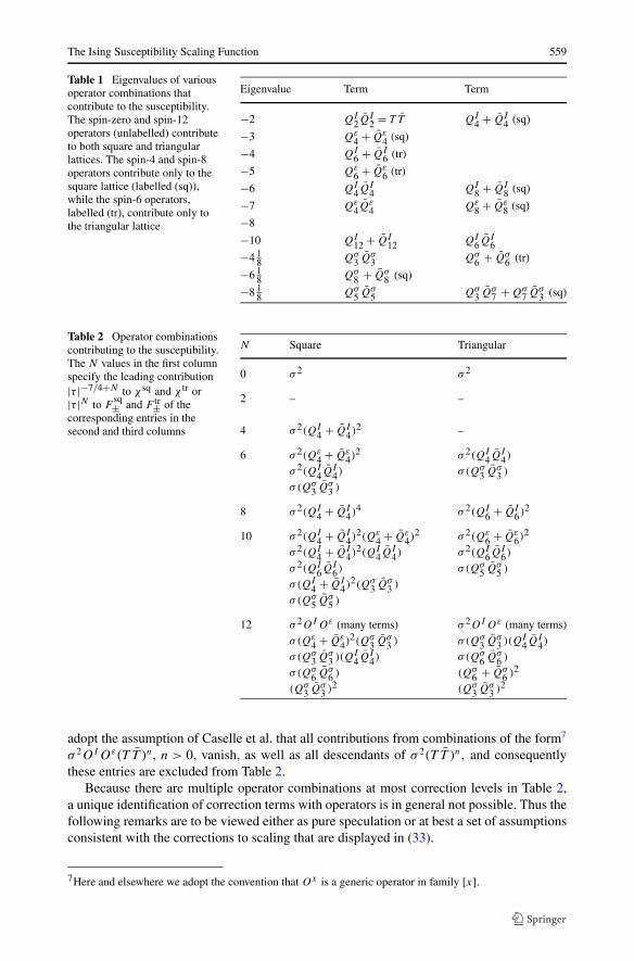
adopt the assumption of Caselle et al. that all contributions from combinations of the form7

σ 2OIOε(T T )n, n > 0, vanish, as well as all descendants of σ 2(T T )n, and consequentlythese entries are excluded from Table 2.

Because there are multiple operator combinations at most correction levels in Table 2,a unique identification of correction terms with operators is in general not possible. Thus thefollowing remarks are to be viewed either as pure speculation or at best a set of assumptionsconsistent with the corrections to scaling that are displayed in (33).

7Here and elsewhere we adopt the convention that Ox is a generic operator in family [x].

560 Y. Chan et al.

1. The corrections observed in (33) are consistent with the conjecture that all operator com-binations of the form Oσ OI , Oσ Oε or Oσ OIOε are rational multiples of the leading or-der contribution of Oσ . Furthermore these multipliers are the same above and below Tc.This makes these contributions particularly hard to distinguish from the scaling fields as-sociated with the leading contribution. For example, the rational coefficient 11/7680 of τ 6

in �Fsq± in (33) is very likely a combination of a direct contribution from σ 2(Qε

4 + Qε4)

2

and a scaling field correction from the σ 2(QI4 + QI

4)2 term, whose leading contribution

is at order τ 4.2. We identify all irrational corrections with σ -field operators. Specifically, contributions

proportional to C6± with σ(Qσ3 Qσ

3 ) and those proportional to C10± with σ(Qσ5 Qσ

5 ). Theambiguity in C6± and C10± as discussed following (8)–(12) is relevant in the presentcontext. A part of C6± might be a rational number associated with σ 2(QI

4QI4) and this

would further complicate the interpretation of the 11/7680 coefficient of τ 6 described initem 1.

3. The coefficients of C6± in (33) on the different lattices are, after dividing out the leadingτ 6 term, 1 − 4973τ 2/5040 + · · · (square), 1 − 403τ 2/400 + · · · (triangular) and 1 −409τ 2/400 + · · · (honeycomb). Because these are all different, we must conclude thatthe scaling function associated with σ(Qσ

3 Qσ3 ) is lattice dependent. An analogy is the

difference seen in the F± scaling function on the kagomé lattice as seen in (36). It is theequality of F± on the square, triangular and honeycomb lattices to O(τ 3) that is to beconsidered as “accidental” and not generic.

4. The very particular structure of the short-distance terms, given in (2) is not explicitlypredicted by CFT. Rather, since the primary logarithm, responsible for the specific heatbehaviour, is due to a resonance between the thermal and identity operator [21], we mightexpect additional multiple resonances, giving rise to higher powers of logarithms. Theseare indeed observed, but it does not appear to be possible to associate particular operatorswith these terms—at least not by our naive method of just power counting.

5. Table 2 shows two new distinct σ -field operators at order τ 12. If, as we have conjecturedin item 2, each is associated with a new irrational C± then we can no longer make anyunique identifications as we did for C6± and C10±. For all terms in F± beyond τ 10 we areleft only with the numerical coefficients tabulated in Appendix A.

3 Generation of Series

3.1 Quadratic Recurrences and Z-Invariance

The algorithm deriving the susceptibility series for the isotropic square lattice Isingmodel [4], with k = sinh2(2βJ ), was rather simple using [24]8

k[C(M,N)2 − C(M,N − 1)C(M,N + 1)]+ [C∗(M,N)2 − C∗(M − 1,N)C∗(M + 1,N)] = 0,

k[C(M,N)2 − C(M − 1,N)C(M + 1,N)]+ [C∗(M,N)2 − C∗(M,N − 1)C∗(M,N + 1)] = 0,

(41)

8For the uniform rectangular Ising model, using the methods of their lattice-Painlevé III paper [25], McCoy

and Wu [26] have generalised (41) to the so-called λ-extended version, in which the coefficient of λj inC(M,N;λ) is the j -particle contribution to the pair correlation function C(M,N). Equations like (41) alsoexist for n-point correlation functions [27].

The Ising Susceptibility Scaling Function 561

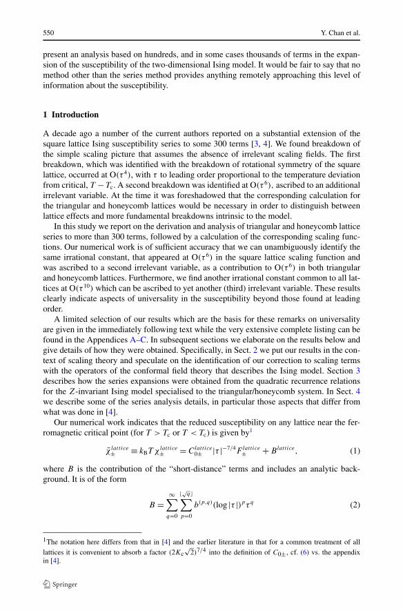
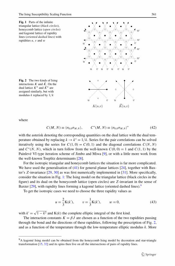
Fig. 1 Parts of the infinitetriangular lattice (black circles),honeycomb lattice (open circles)and kagomé lattice of rapiditylines (oriented dashed lines) withrapidities u, v and w

Fig. 2 The two kinds of Isinginteractions K and K . On thedual lattice K∗ and K∗ areassigned similarly, but withmodulus k replaced by 1/k

where

C(M,N) ≡ 〈σ0,0σM,N 〉, C∗(M,N) ≡ 〈σ0,0σM,N 〉∗ (42)

with the asterisk denoting the corresponding quantities on the dual lattice with the dual tem-perature obtained by replacing k → k∗ = 1/k. Series for the pair correlations can be solvediteratively using the series for C(1,0) = C(0,1) and the diagonal correlations C(N,N)

and C∗(N,N), which in turn follow from the well-known C(0,0) = 1 and C(1,1) by thePainlevé VI type iteration scheme of Jimbo and Miwa [9], or with a little more work fromthe well-known Toeplitz determinants [28].

For the isotropic triangular and honeycomb lattices the situation is far more complicated.We have used the generalisation of (41) for general planar lattices [24], together with Bax-ter’s Z-invariance [29, 30] as was first numerically implemented in [31]. More specifically,consider the situation in Fig. 1: The Ising model on the triangular lattice (black circles in thefigure) and its dual on the honeycomb lattice (open circles) are Z-invariant in the sense ofBaxter [29], with rapidity lines forming a kagomé lattice (oriented dashed lines).9

To get the isotropic cases we need to choose the three rapidity values as

u = 2

3K(k′), v = 1

3K(k′), w = 0, (43)

with k′ = √1 − k2 and K(k) the complete elliptic integral of the first kind.

The interaction constants K = βJ are chosen as a function of the two rapidities passingthrough the bond and the directions of these rapidities, following the prescription of Fig. 2,and as a function of the temperature through the low-temperature elliptic modulus k. More

9A kagomé Ising model can be obtained from the honeycomb Ising model by decoration and star-triangletransformation [15, 32] and its spins then live on all the intersections of pairs of rapidity lines.

562 Y. Chan et al.

precisely,

sinh(2K(u,v)

) = sc(u − v, k′) = k−1cs(K(k′) − u + v, k′), (44)

sinh(2K(u, v)

) = k−1cs(u − v, k′) = sc(K(k′) − u + v, k′), (45)

where sc(v, k) = sn(v, k)/cn(v, k) = 1/cs(v, k). For the dual lattice with k∗ = 1/k beingthe high-temperature elliptic modulus and sinh(2K∗) sinh(2K) = 1, we have

sinh(2K∗(u, v)

) = k sc(u − v, k′) = cs(K(k′) − u + v, k′), (46)

sinh(2K∗(u, v)

) = cs(u − v, k′) = k sc(K(k′) − u + v, k′). (47)

For the triangular lattice we have (44) with u − v = K(k′)/3 or (45) with u − v = 2K(k′)/3,whereas for the honeycomb lattice (44) with u−v = 2K(k′)/3 or (45) with u−v = K(k′)/3.Therefore, it is easy to see that the resulting interactions are isotropic for both lattices.

As the correlation functions only depend on differences of the rapidities, we can add anarbitrary common constant to all of them [29]. Changing the direction of a rapidity line isequivalent to adding ±K(k′) to its rapidity [30]. Together with (43), these two propertiesshow that we have invariance under a rotation by 60° for the rapidity lattice, implying therequired rotation invariance over 60° for the pair correlations on the triangular lattice (orover 120° for the honeycomb lattice). In addition we have several reflection properties.

Most importantly, Baxter’s Z-invariance implies that the pair correlation functions, apartfrom their dependence on the modulus k, only depend on the rapidities that pass between thetwo spins [29], where we have to make all rapidities pass in the same direction by addingthe above ±K(k′) to a rapidity that passes in the opposite direction [30]. Thus we onlyneed to determine universal functions g(u1, . . . , u2m; k) and g∗(u1, . . . , u2m; k) giving thepair correlations on the lattice (T < Tc) and the dual lattice (T > Tc).10 These functions areinvariant under any permutation, or under simultaneous translation by a same amount, of allrapidities [29]. As the rapidities uj can only take the three values (43), we find it convenientto introduce the abbreviations [31]

g[Nu,Nv,Nw] ≡ g(u1, . . . , u2m; k) = g[Nw,Nv,Nu],g∗[Nu,Nv,Nw] ≡ g∗(u1, . . . , u2m; k) = g∗[Nw,Nv,Nu],

(48)

where

Nu = #{uj |uj = u}, Nv = #{uj |uj = v}, Nw = #{uj |uj = w}, (49)

counting the number of uj ’s equal u, v, and w. The symmetry under the interchange of Nu

and Nw in (48) corresponds to a reflection symmetry that holds in the isotropic case (43).Another reflection symmetry gives

g[M,N,0] = g[N,M,0] = g[0,M,N ] = g[0,N,M],g[M,0,N ] = g[N,0,M], (50)

g[N,0,0] = g[0,N,0] = g[0,0,N ],and similar relations hold for g∗; these are also reflection symmetries for the uniformanisotropic square lattice case represented in Fig. 3.

10Compared to [10] we have interchanged g and g∗ through this convention.

The Ising Susceptibility Scaling Function 563

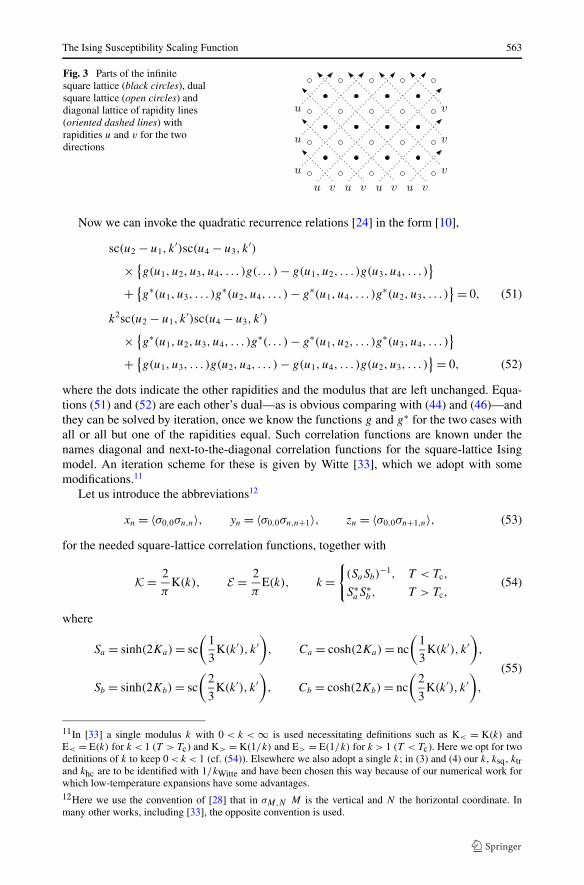
Fig. 3 Parts of the infinitesquare lattice (black circles), dualsquare lattice (open circles) anddiagonal lattice of rapidity lines(oriented dashed lines) withrapidities u and v for the twodirections

Now we can invoke the quadratic recurrence relations [24] in the form [10],

sc(u2 − u1, k′)sc(u4 − u3, k

′)

× {g(u1, u2, u3, u4, . . . )g(. . . ) − g(u1, u2, . . . )g(u3, u4, . . . )

}

+ {g∗(u1, u3, . . . )g

∗(u2, u4, . . . ) − g∗(u1, u4, . . . )g∗(u2, u3, . . . )

} = 0, (51)

k2sc(u2 − u1, k′)sc(u4 − u3, k

′)

× {g∗(u1, u2, u3, u4, . . . )g

∗(. . . ) − g∗(u1, u2, . . . )g∗(u3, u4, . . . )

}

+ {g(u1, u3, . . . )g(u2, u4, . . . ) − g(u1, u4, . . . )g(u2, u3, . . . )

} = 0, (52)

where the dots indicate the other rapidities and the modulus that are left unchanged. Equa-tions (51) and (52) are each other’s dual—as is obvious comparing with (44) and (46)—andthey can be solved by iteration, once we know the functions g and g∗ for the two cases withall or all but one of the rapidities equal. Such correlation functions are known under thenames diagonal and next-to-the-diagonal correlation functions for the square-lattice Isingmodel. An iteration scheme for these is given by Witte [33], which we adopt with somemodifications.11

Let us introduce the abbreviations12

xn = 〈σ0,0σn,n〉, yn = 〈σ0,0σn,n+1〉, zn = 〈σ0,0σn+1,n〉, (53)

for the needed square-lattice correlation functions, together with

K = 2

πK(k), E = 2

πE(k), k =

{(SaSb)

−1, T < Tc,

S∗aS

∗b , T > Tc,

(54)

where

Sa = sinh(2Ka) = sc

(1

3K(k′), k′

), Ca = cosh(2Ka) = nc

(1

3K(k′), k′

),

Sb = sinh(2Kb) = sc

(2

3K(k′), k′

), Cb = cosh(2Kb) = nc

(2

3K(k′), k′

),

(55)

11In [33] a single modulus k with 0 < k < ∞ is used necessitating definitions such as K< = K(k) andE< = E(k) for k < 1 (T > Tc) and K> = K(1/k) and E> = E(1/k) for k > 1 (T < Tc). Here we opt for twodefinitions of k to keep 0 < k < 1 (cf. (54)). Elsewhere we also adopt a single k; in (3) and (4) our k, ksq, ktrand khc are to be identified with 1/kWitte and have been chosen this way because of our numerical work forwhich low-temperature expansions have some advantages.12Here we use the convention of [28] that in σM,N M is the vertical and N the horizontal coordinate. Inmany other works, including [33], the opposite convention is used.

564 Y. Chan et al.

for T < Tc, and

S∗a = sinh(2Ka) = cs

(2

3K(k′), k′

), C∗

a = cosh(2Ka) = ns

(2

3K(k′), k′

),

S∗b = sinh(2Kb) = cs

(1

3K(k′), k′

), C∗

b = cosh(2Kb) = ns

(1

3K(k′), k′

),

(56)

for T > Tc. Equations (54)–(56) define the rescaled complete elliptic integrals and the hy-perbolic sines and cosines of twice the horizontal and vertical reduced interaction constantsin terms of elliptic modulus k. Here Ka is also the reduced interaction energy Ktr of thetriangular lattice and Kb is the Khc of the honeycomb lattice. Duality between low- andhigh-temperature phases is described by the replacements

k∗ = 1/k, K∗ = kK, E ∗ = k−1(

E − (1 − k2)K), (57)

S∗a = 1

Sb

, S∗b = 1

Sa

, C∗a = Cb

Sb

, C∗b = Ca

Sa

. (58)

It is easy to check that the dual of the dual gives the original quantities back (X∗∗ = X).In general, the nearest-neighbour correlations of the square lattice involve the complete

elliptic integral of the third kind �1(n, k) [28, 30, 31, 33],13

y0 = 2

π

Cb

S2aSb

[C2

a�1(1/S2b , k) − K(k)

], (59)

z0 = 2

π

Ca

SaS2b

[C2

b�1(1/S2a , k) − K(k)

], (60)

for T < Tc, and14

y∗0 = 2

π

C∗b

S∗a

[C∗2

a �1(S∗2a , k) − K(k)

], (61)

z∗0 = 2

π

C∗a

S∗b

[C∗2

b �1(S∗2b , k) − K(k)

], (62)

for T > Tc. However, because we have Ka = Ktr, Kb = Khc and the dual/star-triangle rela-tion (5) or equivalently

Cb = Ca

Ca − Sa

= Ca(Ca + Sa), (63)

these correlations y0 and z0 (and also y∗0 and z∗

0) are also the nearest-neighbour correlationsof the isotropic triangular and honeycomb lattices. This in turn means they only involve thecomplete elliptic integral of the first kind [34–36].

To make this more explicit, use [37]

�1

(−k2sn2(a, k), k) = K(k)

[1 + sn(a, k)

cn(a, k)dn(a, k)Z(a, k)

], (64)

13See (4.3a) and (4.3b) of Chap. 8 of [28], correcting a minor misprint, or (52) of [33], identifying �1(n, k) =�(−n, k).14Here, as in (56), the asterisk indicates that the RHS is the high-temperature expression.

The Ising Susceptibility Scaling Function 565

where

Z(a, k) = �′(a, k)

�(a, k)(65)

is Jacobi’s Zeta function and [38]

�(u, k) = θ4(z, q) =∞∑

n=−∞(−1)nqn2

e2inz,

z = πu

2K(k), q ≡ e−πK(k′)/K(k). (66)

When a is a rational multiple of iK(k′), say a = miK(k′)/n, then Z(a, k) can be expandedin powers of q1/n. It can even be calculated in terms of K(k), Sa and Sb using the additionformula [37, 38]

Z(u + a, k) = Z(u, k) + Z(a, k) − k2 sn(u, k) sn(a, k) sn(u + a, k), (67)

and

Z(2iK(k′), k) = − π i

K(k), Z

(1

2iK(k′), k

)= 1

2i(1 + k) − π i

4K(k). (68)

Setting u = 2a = 4A, u = a = 2A or u = a = A ≡ iK(k′)/3 in (67), we find

Z(A, k) = − π i

6K(k)− 1

6k2sn3(2A,k) + 1

2k2sn2(A, k) sn(2A,k),

Z(2A,k) = − π i

3K(k)− 1

3k2sn3(2A,k), A ≡ 1

3iK(k′).

(69)

Here, using Jacobi’s imaginary transformation [38],

sn(A, k) = i sc

(1

3iK(k′), k′

)= iSa = i

kSb

, (70)

sn(2A,k) = i sc

(2

3iK(k′), k′

)= iSb = i

kSa

. (71)

Therefore,

y0 = 1

3

Ca

Sa

+[

Cb

Sb

+ 1

2

Ca

SaSb

− 1

6

SbCa

S 3a

]K,

z0 = 2

3

Cb

Sb

+[

Ca

Sa

− 1

3

Cb

S 2a

]K, for T < Tc,

(72)

and

y∗0 = 1

3Cb +

[Ca

SaSb

+ 1

2

Cb

Sb

− 1

6

SbCb

S 2a

]K,

z∗0 = 2

3Ca +

[Cb

SaSb

− 1

3

SbCa

S 2a

]K, for T > Tc.

(73)

Results (72) and (73) differ by duality as defined in (57) and (58).

566 Y. Chan et al.

We next rewrite (72) and (73) using (63) or alternatively using Ka = Ktr and Kb = Khc

with the explicit connections to u and z given in (4) and (5).15 With the latter we obtain

y0 = 1 + u

3(1 − u)

[1 + 2(1 − 3u)√

(1 − u)3(1 + 3u)K

], (74)

z0 = 1 + z2

3(1 − z2)

[2 + (1 + z)(1 − 4z + z2)

(1 − z)3K

], (75)

which can be compared directly with the internal energy results in Table I of Houtap-pel [34].16 These results are also the basis for our (26) and (27); the equality follows by using(22) and the low-temperature Landen transformation from (23) to yield I (τ ) = 2

√k K.

We can also rewrite (44) and (54) of [33]. Then the first few square-lattice correlations inthe low-temperature phase are

x0 = 1, x1 = E , (76)

y0 = Ca

3Sa

(1 − (Ca − 2Sa)(Ca + Sa)

2 K∗), (77)

z0 = Cb

3Sb

(2 + (Cb − 2)(Cb + 1)2

S3b

K)

, (78)

y1 =(

E − Sb

Sa

E ∗)

y0 + Cb

Sa

E E ∗, (79)

z1 =(

E − Sa

Sb

E ∗)

z0 + Ca

Sb

E E ∗, (80)

whereas the corresponding quantities in the high-temperature phase are

x∗0 = 1, x∗

1 = E ∗, (81)

y∗0 = 1

3Cb

(1 − (Cb − 2)(Cb + 1)2

S3b

K)

, (82)

z∗0 = 1

3Ca

(2 + (Ca − 2Sa)(Ca + Sa)

2 K∗), (83)

y∗1 =

(E ∗ − Sb

Sa

E)

y∗0 + SbCa

Sa

E E ∗, (84)

z∗1 =

(E ∗ − Sa

Sb

E)

z∗0 + SaCb

Sb

E E ∗. (85)

These results are fully consistent with duality defined in (57) and (58). In addition, we havez∗

0 = Ca − Say0 and y∗0 = Cb − Sbz0, in agreement with (11) in [24].

15Cf. also (106) and (107) in the following section.16The results of Wannier [35] and Newell [36] differ by Landen transformations [38]

kNewell = 2√

k

1 + k, kWannier = − 1 − k′

1 + k′ .

The Ising Susceptibility Scaling Function 567

Witte’s initial conditions, (40) and (42) in [33], can be rewritten as

r0 = 1, r0 = 1, (86)

r1 = −2k

3+ E ∗

3E, r1 = E ∗

E, (87)

and

r∗0 = 1, r∗

0 = 1, (88)

r∗1 = − 2

3k+ E

3E ∗ , r∗1 = E

E ∗ . (89)

Then further quantities can be found systematically using

(2j + 3)(1 − rj rj )rj+1 = 2j(k + k−1 + (2j − 1)rj rj−1

)rj

− (2j − 3)(1 + (2j − 1)rj rj

)rj−1, (90)

(2j + 1)(1 − rj rj )rj+1 = 2j(k + k−1 − (2j − 3)rj rj−1

)rj

− (2j − 1)(1 − (2j + 1)rj rj

)rj−1, (91)

and the identical equations for r∗j and r∗

j , see (38) and (39) in [33]. The further diagonal andnext-to-the-diagonal correlations follow using

xj+1 = x2j

xj−1(1 − rj rj ), (92)

yj+1 = xj+1

xj

(1 − rj+1

rj

Sb

Sa

)yj + x2

j+1

x2j

rj+1

rj

Sb

Sa

yj−1, (93)

zj+1 = xj+1

xj

(1 − rj+1

rj

Sa

Sb

)zj + x2

j+1

x2j

rj+1

rj

Sa

Sb

zj−1, (94)

and their dual versions obtained by replacing all quantities by their ∗ versions. These lastfew equations can be found combining (31), (36), (59), (63) and (64) of [33]. For the currentpurpose one only needs zn and z∗

n for n = 0.We have now all equations from the square-lattice Ising model needed to generate g and

g∗ with all or all but one of the rapidities equal in a form that makes the lattice symmetriesand duality manifest. Thus we can now construct a “polynomial-time” algorithm for thehigh- and low-temperature series coefficients for the susceptibility of the isotropic Isingmodel on triangular, honeycomb (and kagomé) lattices. For efficiency of the algorithm, wedesire series with only integer coefficients. Series in the low-temperature u = exp(−4Ktr)

are certainly acceptable; because the coefficients in these series can be reduced to latticecounts, they are necessarily integer. A useful alternative in the square lattice case [4] wasthe elliptic parameter k. The corresponding alternative here suggested by the ktr(u) relation(4) is an expansion in the variable k = (k2/16)1/3. Inversion of ktr(u) results in the series

u = k − 2k3 + 8

3k4 + 3k5 − 16k6 + 152

9k7 + 40k8 − 161k9 + 11200

81k10 + · · · (95)

and although the rationals in (95) can be eliminated by the change k → k/3 the coefficientsin any correlation function series in k will grow unacceptably rapidly. A third alternative is

568 Y. Chan et al.

expansion in q1/3 where q is the elliptic nome. This is suggested by k = (k2/16)1/3 and theknown expansion k2/16 = q − 8q2 + · · · .

All our elliptic functions have natural expansions in terms of the elliptic nome

q = exp

(−πK(k′)

K(k)

), (96)

using Jacobi theta functions, i.e. [38]

k =[

θ2(0, q)

θ3(0, q)

]2

, k′ =[

θ4(0, q)

θ3(0, q)

]2

, (97)

K = [θ3(0, q)

]2, E = [

θ3(0, q)]2 − θ ′′

4 (0, q)

θ4(0, q)[θ3(0, q)]2. (98)

Also, from (55),

Sa = −i sn

(1

3i K(k′), k

), Ca = cn

(1

3i K(k′), k

),

Sb = −i sn

(2

3i K(k′), k

), Cb = cn

(2

3i K(k′), k

),

(99)

using Jacobi’s imaginary transformation. In terms of theta functions,

Sa,b = −i√k

θ1(za,b, q)

θ4(za,b, q), Ca,b =

√k′

k

θ2(za,b, q)

θ4(za,b, q), (100)

with

za = π

2K(k)

i K(k′)3

, zb = 2za, eiza = q1/6, eizb = q1/3. (101)

From the above we expect to end up with expansions in the nome

q = exp

(−πK(k′)

3K(k)

)= q1/3 (102)

and this is the good expansion variable that we used.17

For expansions in terms of the nome it is also advantageous to break the symmetry defin-ing

rj = (−k)jρj , rj = (−k)−j ρj , (103)

and similar for r∗j and r∗

j , in order to avoid square roots of the nome.

17There are many other cases where series in the nome are advantageous. Whenever all rapidity differences

are of the form mK(k′)/n with fixed integer n, we can expand the susceptibility in powers of q = q1/n, seethe text following (66).

The Ising Susceptibility Scaling Function 569

3.2 Alternative Expressions

The functions sc( 13 K(k′), k′) and sc( 2

3 K(k′), k′) have an algebraic representation in k whichone can obtain by expanding identities such as cs( 1

3 K(k) + 13 K(k) + 1

3 K(k), k) = 0 usingstandard addition formulae and then solving the resulting quartic equation for sc( 1

3 K(k), k).One finds

sc

(1

3K(k′), k′

)= 1√

Rk, sc

(2

3K(k′), k′

)=

√R

k, (104)

where

R = X +√

3 − X2 + (k−1 + k)/X, X =√

1 + ((k−1 − k)2/4

)1/3. (105)

Note that R is self-dual, i.e. invariant under the replacement k → 1/k, whilesc( 1

3 K(k′), k′) ↔ cs( 23 K(k′), k′). If we take k = ktr, the low-temperature elliptic parame-

ter (4), then one can verify

1√Rk

= 1 − u

2√

u≡ sinh(2Ktr) (106)

and√

R

k=

√(1 − u)(1 + 3u)

2u= 1 − z2

2z≡ sinh(2Khc), (107)

where in (107) we have used (5) for u(z). In this way we confirm directly from (104)–(107)and the definitions (55) that Ka = Ktr and Kb = Khc.

The expansions in the (cube root) nome q = exp(−πK′/3K) described in the precedingsection can be applied to (Ca − Sa)

2 to give directly u = u(q). We obtain the formula

u = q

( ∞∑

n=0

(q4n − q8n+2)/(1 − q12n+6)

)2/( ∞∑

n=0

q3n(n+1)

)4

= q − 2q3 + 3q5 − 4q7 + 7q9 − 12q11 + 17q13 − 24q15 + · · · , (108)

which explicitly shows u(q) is an integer series. Whether correlation function series in u

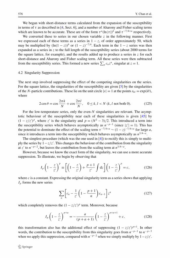
or q will show the slowest growth in the magnitude of the series coefficients depends onthe singularity structure of the correlation functions. Now the correlation functions as se-ries in u have radius of convergence 1/3 governed both by the ferromagnetic singularity atu = 1/3 and an unphysical singularity at u = −1/3. There are other more distant complexsingularities and what we have found numerically and describe in Sect. 4.2 is that there is aclose analogy with the singularities on the square lattice. Indeed we conjecture that |ktr| = 1is dense with singularities and part18 of a natural boundary for the triangular lattice. Nowthe circle |ktr| = 1 maps to arcs in the q-plane with distance to the origin bounded belowby exp(−π/3) = 0.3509 . . . and it is this distance that fixes the radius of convergence ofthe q series. It implies that asymptotically in N we have terms of magnitude ∼ 2.85N qN

compared to ∼ 3NuN . As an example of what we observe in practice, the coefficients in theseries expansion of the low-temperature triangular lattice susceptibility are, at the largest

18For the complete natural boundary see Fig. 5 in Sect. 4.2.

570 Y. Chan et al.

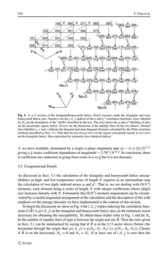
Fig. 4 A π/3 section of the triangular/honeycomb lattice. Small triangles mark the triangular and evenhoneycomb lattice sites. Numbers are the i, k, j indices of the g and g∗ correlation functions. Lines labelledby Ns are the boundaries of the “shells” described in the text. The inset shows the g and g∗ labelling of siteson the anisotropic square lattice. Vectors are the directions of the rapidity lines on the two lattices. Dashedlines labelled x, y and z indicate the diagonal and near diagonal elements calculated by the Witte recursionrelations described in Sect. 3.1. Note that the two lowest rows on the square correspond exactly to two rowson the triangular lattice. Sites equivalent by symmetry have identical indices

N we have available, dominated by a single u-plane singularity pair (u − (1 ± 2i)/5)13/2

giving a q series coefficient dependence of magnitude ∼ 2.78N/N15/2. In conclusion, thereis coefficient size reduction in going from series in u to q but it is not dramatic.

3.3 Computational Details

As discussed in Sect. 3.1 the calculation of the triangular and honeycomb lattice suscep-tibilities as high- and low-temperature series of length N requires as an intermediate stepthe calculation of two triply indexed arrays g and g∗. That is, we are dealing with O(N3)

elements, each element being a series of length N with integer coefficients whose (digit)size increases linearly with N . Fortunately this O(N5) memory requirement can be circum-vented by a careful sequential arrangement of the calculation and the description of this withemphasis on the storage structure we have implemented is the content of this section.

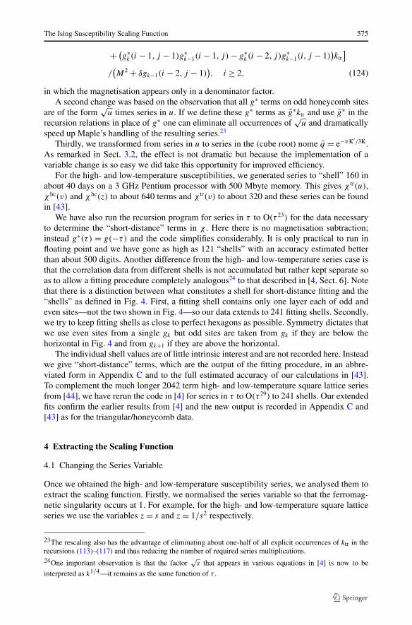
To begin the discussion we show in Fig. 4 the i, k, j triples indexing the correlation func-tions C( �R) ≡ g(i, k, j) at the triangular and honeycomb lattice sites on the minimum sectornecessary for obtaining the susceptibility. To obtain these triples refer to Fig. 1 and let Nα

be the number of rapidity lines of type α between the origin and site �R. Then the rules givenin Sect. 3.1 can be summarised by saying that if �R is in the π/3 sector above (below) thehorizontal through the origin then g(i, k, j) = g(Nw,Nv,Nu) (= g(Nw,Nu,Nv)). Clearlyif �R is on the horizontal, Nw = 0 and Nu = Nv . If at least one of i, k, j is zero then the

The Ising Susceptibility Scaling Function 571

corresponding g is also a correlation function on the anisotropic square lattice. For exam-ple, if i = 0, then in g(0, k, j) we can identify j = nx and k = ny where nx and ny arethe Cartesian coordinates of sites in the first quadrant of the square lattice obtained by ro-tating that shown in Fig. 4 clockwise by π/4. In the fourth quadrant of this rotated latticeg(i,0, j) = g(−ny,0, nx). With the exception of g(1,0,1) only elements g(0, ny, nx) areneeded as initial conditions for the recursion relations for the general C( �R) on the triangularand honeycomb lattices.

It is worth remarking that the correlations g(0, n,n) on the triangular lattice diagonal canbe calculated as Toeplitz determinants [39] and we have used this as an important checkof our computations. We also note that of the symmetries (48) and (50) satisfied by theg(i, k, j), two in particular that we use below are g(i, k, j) = g(j, k, i) and g(0, k, j) =g(0, j, k).

One observes in Fig. 4 that within each “shell” Ns , that is, sites between lines Ns − 1and Ns , the central k index is either 2Ns − 2 or 2Ns − 1. It turns out that with a few ex-ceptions, an array at fixed k can be computed from elements in an array with index k − 1.Proceeding sequentially through “shells”, or equivalently k, reduces the memory require-ment from O(N5) to O(N4). It also has the advantage of allowing the calculation to bestopped and restarted if necessary at convenient intervals and makes calculation with an N

of several hundred to a thousand practical.We take the array19 g(i, k, j) ≡ gk(i, j) indexed—using Maple notation—in the dou-

ble sequence seq(seq(gk(i,i+2*j),j=0...Ns-i),i=0...Ns) for even k =2Ns − 2 as constituting “shell” Ns(a). The array g(i, k, j) ≡ gk(i, j) with odd k = 2Ns − 1and indexed as seq(seq(gk(i,i+2*j+1),j=0...Ns-i),i=0...Ns) constitutes“shell” Ns(b). The indexing for both arrays is such that j ≥ i, i + j ≤ k + 2, and satisfiesthe requirement that i + k + j be even. As a specific example of this indexing, the Ns = 3case is illustrated as (109)

(g4) 040

↑︷︸︸︷042

⇑︷︸︸︷044 046

↑︷︸︸︷141

⇑︷︸︸︷143

↑︷︸︸︷145

⇑︷︸︸︷242

↑︷︸︸︷244

↑︷︸︸︷343 (3a)

(109)

(g5) 051

↑︷︸︸︷053

⇑︷︸︸︷055 057

↑︷︸︸︷152

⇑︷︸︸︷154

↑︷︸︸︷156

⇑︷︸︸︷253

↑︷︸︸︷255

↑︷︸︸︷354 (3b)

with gk label on the left and “shell” label on the right. Both Ns(a) and Ns(b) arrays areof length L = (Ns + 1)(Ns + 2)/2 and we introduce a third notation, namely the singleindexed gk(�), � = 1 . . .L. The physical elements on the lattice are only a subset of 3Ns − 1elements in each array. Specifically, the triangular and even honeycomb sites are at locations� = L−1−n(n+1)/2, n = 1 . . .Ns and are indicated by the double arrows in (109). The oddhoneycomb sites below the horizontal in Fig. 4 are at � = L − n(n + 1)/2, n = 0 . . .Ns − 1while those above are at � = L − 2 − n(n + 1)/2, n = 2 . . .Ns . Both sets are indicated bysingle arrows in (109).

We also require linear arrays which for identification purposes we will denote as dk withthe even and odd k arrays being distinct. The array d0 is initialised by elements from theanisotropic square lattice array x described in Sect. 3.1; d1 by the corresponding elementsfrom y. In subsequent calculations, dk−2 will be renamed dk and certain elements changedby an in-place replacement determined by the quadratic recursion formulae. Details will

19While we only refer to an array g here, there is a strictly parallel dual array g∗ . It is to be understood thatsuch convention applies throughout this section.

572 Y. Chan et al.

be described below; for now it is enough to know that the changes will maintain dk(1) =g(0, k + 2, k mod 2), dk(2) = g(0, k, k + 2) and dk(3) = g(0, k, k + 4). The dk(n), n >

Ns + 1 remain unchanged from the initialisations

(d0) 020 002 004 006 008 . . . (g0)

⇑︷︸︸︷000 002

↑︷︸︸︷101 (1a)

(110)

(d1) 031 013 015 017 019 . . . (g1)

⇑︷︸︸︷011 013

↑︷︸︸︷112 (1b)

where arrows indicate physical site elements as in (109). The underlines indicate elementsthat have been copied, specifically d0(n) = xn−1 and d1(n) = yn−1 for n > 1. Also, the ele-ments in g0 are x0, x1 and z0 while the first two in g1 are y0 and y1. A special remark is inorder for elements d0(1) and d1(1)—these are equal respectively to d0(2) and d1(2) becauseof the symmetry gk(0, j) = gj (0, k). The third element in g1 is given by

g(1,1,2) = g(0,1,1)g(1,0,1) + g∗(0,1,1)(g∗(1,0,1) − g∗(0,0,2))ktr (111)

which is a special case of the recursion equation (116). Note that the dual of (111) requiresboth g ↔ g∗ and ktr → 1/ktr.

This completes the initialisation except for combining the physical site elements in (110),with appropriate multiplicity factors, into (summed) correlation functions from which sus-ceptibilities will be determined as a very last step. These functions are chosen to distinguishbetween even and odd sites; given the initialisation (110) we set

Ce = δg0(1) + 6δg1(1), Co = 3δg0(3) + 6δg1(3),

C∗e = g∗

0(1) + 6g∗1(1), C∗

o = 3g∗0(3) + 6g∗

1(3).(112)

Each δg in (112) is the magnetisation subtracted g − M2 which applies only to the low-temperature variables and not the high-temperature duals.

The recursion in which new gk are calculated starts with k = 2 and Ns = 2. In the gen-eral case the first element of gk is initialised by copying from dk−2, specifically gk(1) =dk−2(1) = g(0, k, k mod 2). We then proceed sequentially from the gk(2) to the finalgk(L),L = (Ns + 1)(Ns + 2)/2, using the quadratic recursion relations for each. Unlessforced otherwise, we use only elements from gk and gk−1 to minimise what is kept in mem-ory and this requires that different forms of the recursion relations be used depending on thei, j combination in gk(i, j). In the order used, these are20

gk(0, j) = [gk−1(0, j − 1)2 + (g∗k−1(0, j − 1)2

− g∗k (0, j − 2)g∗

k−2(0, j))Rktr]/gk−2(0, j − 2), 1 < j ≤ k, (113)

gk(0, k + 2) = [gk−1(0, k + 1)2 + (g∗k−1(0, k + 1)2

− g∗k (0, k)d∗

k−2(3))Rktr]/gk−2(0, k), (114)

gk(1,1) = [gk−1(0,1)2 − (g∗k−1(0,1)2

− g∗k (0,0)g∗

k−2(1,1))Rktr]/gk−2(0,0), (115)

20As noted in the context of (109) each equation is to be understood as a pair. Here the second member isobtained by the interchange gk ↔ g∗

kand replacements d∗ → d and ktr → 1/ktr.

The Ising Susceptibility Scaling Function 573

gk(1, j) = [gk(0, j − 1)gk−1(1, j − 1)

+ (g∗k (0, j − 1)g∗

k−1(1, j − 1) − g∗k (1, j − 2)g∗

k−1(0, j))ktr]/gk−1(0, j − 2), j > 1, (116)

gk(i, j) = [gk(i − 1, j − 1)gk−1(i − 1, j)

+ (g∗k (i − 1, j − 1)g∗

k−1(i − 1, j) − g∗k (i − 2, j)g∗

k−1(i, j − 1))ktr]/gk−1(i − 2, j − 1), i ≥ 2, (117)

where the (self-dual) multiplier R is given in (105) or, more simply, as R = Sb/Sa by com-bining (106) and (107). The j index in these recursion equations increments in steps of twoto maintain i + j + k even, a condition that also eliminates (115) unless k is even. Indexingfunctions are easily established which relate the location of the right hand side elements in(113)–(117) to those on the left; this is a coding detail that we do not give here except toremark that the symmetry gk(i, j) = gk(j, i) may have to be invoked to locate an element.The special element d∗

k−2(3) in (114) is g∗(0, k − 2, k + 2) which in our construction of thegk−2 array was explicitly excluded from being one of the elements. As an observation onmemory requirements, only the first Ns elements of array gk−2 are required for implement-ing (113)–(115) so that most of the memory used by gk−2 could be released before the gk

calculation is started. For all further calculations in (116) and (117) only gk−1 need be main-tained in memory. In fact with a small location offset of 2Ns + 1 the replacement gk−1 → gk

could be done in-place and thus reduce memory requirements even further. On completionof the gk calculation in (113)–(117) the gk elements corresponding to physical lattice sitesare accumulated into the C and C∗ as in (112) with appropriate attention to multiplicity.

We must also update the dk−2 array that has just been used in (114) in preparation forsubsequent iterations in k. The dk , and for completeness the relevant gk , are shown in (118)

(d0) 020 002 004 006 008 . . . (g0)

⇑︷︸︸︷000 002

↑︷︸︸︷101 (1a)

(d1) 031 013 015 017 019 . . . (g1)

⇑︷︸︸︷011 013

↑︷︸︸︷112 (1b)

(g2)

↑︷︸︸︷020

⇑︷︸︸︷022 024

⇑︷︸︸︷121

↑︷︸︸︷123

↑︷︸︸︷222 (2a)

(d2) 040 024 026 006 . . .

(g3)

↑︷︸︸︷031

⇑︷︸︸︷033 035

⇑︷︸︸︷132

↑︷︸︸︷134

↑︷︸︸︷233 (2b)

(d3) 051 035 037 017 . . .

(g4) 040

↑︷︸︸︷042

⇑︷︸︸︷044 046

↑︷︸︸︷141

⇑︷︸︸︷143

↑︷︸︸︷145

⇑︷︸︸︷242

↑︷︸︸︷244

↑︷︸︸︷343 (3a)

(d4) 060 046 048 028 008 . . .

(g5) 051

↑︷︸︸︷053

⇑︷︸︸︷055 057

↑︷︸︸︷152

⇑︷︸︸︷154

↑︷︸︸︷156

⇑︷︸︸︷253

↑︷︸︸︷255

↑︷︸︸︷354 (3b)

(d5) 071 057 059 039 019 . . .

(g6) 060 062

↑︷︸︸︷064

⇑︷︸︸︷066 068 161

↑︷︸︸︷163

⇑︷︸︸︷165

↑︷︸︸︷167

↑︷︸︸︷262

⇑︷︸︸︷264

↑︷︸︸︷266

⇑︷︸︸︷363

↑︷︸︸︷365

↑︷︸︸︷464 (4a)

(118)

574 Y. Chan et al.

to illustrate the changes in the dk as one proceeds through to the completion of “shell” 3 andinto “shell” 4. The notation in (118) is as in (109) and (110). Of special note are the under-lined elements in dk, k ≥ 2, and the fact that all changes are made in-place. Specifically thismeans that we first rename dk−2 to dk . Then we copy dk(Ns + 1) to dk(1) since it is neededboth in its original location where it will be overwritten and in a subsequent gk+2 calcula-tion.21 The second copy is from the just completed gk(Ns + 1) to dk(2). The transformationof dk is then completed by a sequence of in-place quadratic recursion transformations ofelements dk(n) starting at n = Ns + 1 and decrementing to n = 3. Each recursion is givenby22

dk(n) = [dk−1(n)2 + (d∗k−1(n)2 − d∗

k (n − 1)d∗k (n + 1))Rktr]/dk(n) (119)

which is in a form identical to (113) including R from (105)–(107). All operations in “loop”k have now been completed and we can restart the overall cycle begun following (112) afterincrementing k → k + 1 and, if the new k is even, Ns → Ns + 1.

On completion of all recursions, high- and low-temperature susceptibility series are gen-erated from the C and C∗ as follows. The triangular lattice susceptibility for T < Tc is givendirectly as

kBT χ tr−(u) = Ce(u) (120)

while that for the honeycomb follows from the duality/star-triangle transformation (5) andis

kBT χhc− (z) = Ce

(u = z/(1 − z + z2)

) ± Co(u = z/(1 − z + z2)

). (121)

Note that both odd and even sites contribute in (121) with the sum for the ferromagnet; thedifference for the antiferromagnet. The results for T > Tc follow by duality and are

kBT χ tr+(v) = C∗

e

(u = v/(1 − v + v2)

), (122)

kBT χhc+ (v) = C∗

e

(u = v2

) + C∗o

(u = v2

), (123)

where v = tanh(K) is the conventional high-temperature variable and K is Ktr or Khc asappropriate. All of these susceptibilities agree with the earlier work by Sykes et al. [40–42].

In our implementation of the above procedure we made full use of Maple’s automaticseries multiplication routines in full integer arithmetic. This is similar to what was donein [4] for the square lattice and allowed us to reach series of adequate length. Howeverwe did introduce several modifications to improve efficiency. First, as also in [4], whengenerating high- and low-temperature series the recursions were set up to deal directly withthe much smaller residuals δg = g − M2. As an example of this change, the recursion (117)becomes

δgk(i, j) = δgk(i − 1, j − 1) + δgk−1(i − 1, j) − δgk−1(i − 2, j − 1)

× [(δgk(i − 1, j − 1) − δgk−1(i − 2, j − 1)

)

× (δgk−1(i − 1, j) − δgk−1(i − 2, j − 1)

)

21There are in general other elements that could be saved for gk+2m, m > 1, but we have opted instead for asmall amount of redundancy in our calculation.22Once again there is a second member obtained by d ↔ d∗ and ktr → 1/ktr which must be done before n isdecremented.

The Ising Susceptibility Scaling Function 575

+ (g∗

k (i − 1, j − 1)g∗k−1(i − 1, j) − g∗

k (i − 2, j)g∗k−1(i, j − 1)

)ktr

]

/(M2 + δgk−1(i − 2, j − 1)

), i ≥ 2, (124)

in which the magnetisation appears only in a denominator factor.A second change was based on the observation that all g∗ terms on odd honeycomb sites

are of the form√

u times series in u. If we define these g∗ terms as g∗ktr and use g∗ in therecursion relations in place of g∗ one can eliminate all occurrences of

√u and dramatically

speed up Maple’s handling of the resulting series.23

Thirdly, we transformed from series in u to series in the (cube root) nome q = e−πK′/3K.As remarked in Sect. 3.2, the effect is not dramatic but because the implementation of avariable change is so easy we did take this opportunity for improved efficiency.

For the high- and low-temperature susceptibilities, we generated series to “shell” 160 inabout 40 days on a 3 GHz Pentium processor with 500 Mbyte memory. This gives χ tr(u),χhc(v) and χhc(z) to about 640 terms and χ tr(v) to about 320 and these series can be foundin [43].

We have also run the recursion program for series in τ to O(τ 23) for the data necessaryto determine the “short-distance” terms in χ . Here there is no magnetisation subtraction;instead g∗(τ ) = g(−τ) and the code simplifies considerably. It is only practical to run infloating point and we have gone as high as 121 “shells” with an accuracy estimated betterthan about 500 digits. Another difference from the high- and low-temperature series case isthat the correlation data from different shells is not accumulated but rather kept separate soas to allow a fitting procedure completely analogous24 to that described in [4, Sect. 6]. Notethat there is a distinction between what constitutes a shell for short-distance fitting and the“shells” as defined in Fig. 4. First, a fitting shell contains only one layer each of odd andeven sites—not the two shown in Fig. 4—so our data extends to 241 fitting shells. Secondly,we try to keep fitting shells as close to perfect hexagons as possible. Symmetry dictates thatwe use even sites from a single gk but odd sites are taken from gk if they are below thehorizontal in Fig. 4 and from gk+1 if they are above the horizontal.

The individual shell values are of little intrinsic interest and are not recorded here. Insteadwe give “short-distance” terms, which are the output of the fitting procedure, in an abbre-viated form in Appendix C and to the full estimated accuracy of our calculations in [43].To complement the much longer 2042 term high- and low-temperature square lattice seriesfrom [44], we have rerun the code in [4] for series in τ to O(τ 29) to 241 shells. Our extendedfits confirm the earlier results from [4] and the new output is recorded in Appendix C and[43] as for the triangular/honeycomb data.

4 Extracting the Scaling Function

4.1 Changing the Series Variable

Once we obtained the high- and low-temperature susceptibility series, we analysed them toextract the scaling function. Firstly, we normalised the series variable so that the ferromag-netic singularity occurs at 1. For example, for the high- and low-temperature square latticeseries we use the variables z = s and z = 1/s2 respectively.

23The rescaling also has the advantage of eliminating about one-half of all explicit occurrences of ktr in therecursions (113)–(117) and thus reducing the number of required series multiplications.24One important observation is that the factor

√s that appears in various equations in [4] is now to be

interpreted as k1/4—it remains as the same function of τ .

576 Y. Chan et al.

We began with short-distance terms calculated from the expansion of the susceptibilityin terms of τ as described in [4, Sect. 6], and a number of Aharony and Fisher scaling termswhich are known to be accurate. These are of the form τ a(ln |τ |)b and τ−7/4+a respectively.

We converted these to series in our chosen variable z in the following manner. Firstwe expressed each of these terms as a series in 1 − z, of order approximately 50, whichmay be multiplied by (ln(1 − z))b or (1 − z)−7/4. Each term in the 1 − z series was thenexpanded as a series in z to the full length of the susceptibility series (about 2000 terms forthe square lattice, for example), and the results added up to produce a series in z for eachshort-distance and Aharony and Fisher scaling term. All these series were then subtractedfrom the susceptibility series. This formed a new series

∑n cnz

n, singular at z = 1.

4.2 Singularity Suppression

The next step involved suppressing the effect of the competing singularities on the series.For the square lattice, the singularities of the susceptibility are given [5] by the singularitiesof the N -particle contributions. These lie on the unit circle |s| = 1 at the points skl = exp(iθ),where

2 cos θ = cos2πk

N+ cos

2πl

N, 0 ≤ k, l < N (k, l not both 0). (125)

For the low-temperature series, only the even-N singularities are relevant. The asymp-totic behaviour of the susceptibility near each of these singularities is given [45] by(1 − z/z′)p , where z′ is the singularity and p = (N2 − 3)/2. This introduced a term intothe susceptibility series which behaves asymptotically as n−p−1 (since |z′| = 1). This hasthe potential to dominate the effect of the scaling term τ−7/4+a ∼ (1 − z)−7/4+a for large a,since it introduces a term into the susceptibility which behaves asymptotically as n3/4−a .

The simplest procedure (which was the one used in [4]) to rectify this is simply to multi-ply the series by 1−z/z′. This changes the behaviour of the contribution from the singularityat z′ to n−p−2, but leaves the contribution from the scaling term at n3/4−a .

However, because we know the exact form of the singularity, we can use a more accuratesuppression. To illustrate, we begin by observing that

Ip

(1 − z

z′

)p

≡[(

1 − z

z′

)+ p + 1

z′

∫dz

](1 − z

z′

)p

= c, (126)

where c is a constant. Expressing the original singularity term as a series shows that applyingIp forms the new series

∑

n

[cn − 1

z′

(1 − p + 1

n

)cn−1

]zn (127)

which completely removes the (1 − z/z′)p term. Moreover, because

Ip

(1 − z

z′

)p+a

= − a

(p + a + 1)

(1 − z

z′

)p+a+1

+ c, (128)

this transformation also has the additional effect of suppressing (1 − z/z′)p+1. In otherwords, the contribution to the susceptibility from this singularity goes from n−p−1 to n−p−3

when we apply this suppression, compared with n−p−2 when we simply multiply by 1−z/z′.

The Ising Susceptibility Scaling Function 577

In addition, applying the integral operator to scaling terms gives

Ip (1 − z)−7/4+a =(

1 − z

z′

)(1 − z)−7/4+a − p + 1

z′(−7/4 + a + 1)(1 − z)−3/4+a, (129)

which still contributes n3/4−a to the asymptotic behaviour of the susceptibility series. So thisoperator suppresses the competing singularity while not asymptotically affecting the scalingterm.

An unfortunate consequence of applying Ip for a complex singularity is that the seriesresulting from (127) has complex coefficients. This can be avoided by observing that sincethe susceptibility is real, for every singularity z′ there is a corresponding singularity of thesame order at z′. Sequentially applying the suppression to both of these singularities resultsin the series

∑

n

[cn − 2 Re z′

|z′|2(

1 − p + 1

n

)cn−1 + 1

|z′|2(

1 − p + 1

n

)(1 − p + 1

n − 1

)cn−2

]zn, (130)

which can be seen to have real coefficients. As all we are doing is applying formula (127)twice for two different singularities, the effects on the singularity and scaling terms that weobserved above still hold.

In practice, we also suppress the higher-order terms (1 − z/z′)p+a for a = 2,4, . . . , usingthe above suppression formula (with p replaced by p + a) for each a. The maximum a thatwe use varies for each singularity and is determined empirically as described below.

For high-temperature series, only the odd-N singularities are relevant. The asymp-totic behaviour of the susceptibility near each of these singularities is given [5] by (1 −z/z′)p ln(1 − z/z′), where p = (N2 − 3)/2. These terms can also be suppressed by the sameformula (127). This can be seen to be true because applying the same integral operator re-sults in an analytic term for integer p (which is true for odd N ). Again, we suppress anumber of higher powers.

In order to determine which singularities should be suppressed and by how much, weapply a Fast Fourier Transform diagnostic, as described in [44, Sect. 7]. We first do a pre-liminary fit of the series to our functions, as described in Sect. 4.3 below, and subtract thefit from the series. The dominant unsuppressed singularity in the remainder is expressed byperiodic behaviour of period 2π/θ , for a singularity located at exp(iθ). By applying FFT tothe remainder, we can observe the periods of the dominant unsuppressed singularities, matchthese to the known singularities, and increase the suppression on these singularities (by sup-pressing more higher-order terms). This is repeated until the remainder has a satisfactorilysmall amplitude.

The analysis of the triangular and honeycomb series is almost identical, though we mustsuppress the appropriate singularities (see [46]). For these lattices, it is conjectured that thesingularities lie on the curve of Matveev and Shrock [47],

1 + 3u2 − 2u(1 − u)x = 0, −3

2≤ x ≤ 3. (131)

We further conjecture that the singularities are given implicitly by this equation when x

takes the values

xklm = cos2πk

N+ cos

2πl

N+ cos

2πm

N, k + l + m ≡ 0 mod N (k, l, m not all 0). (132)

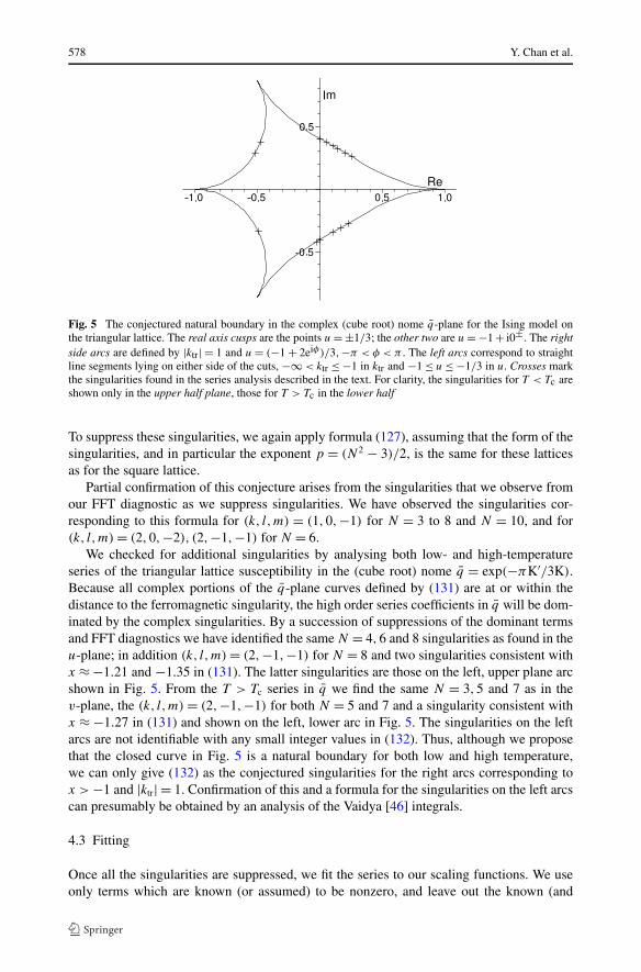
578 Y. Chan et al.

Fig. 5 The conjectured natural boundary in the complex (cube root) nome q-plane for the Ising model onthe triangular lattice. The real axis cusps are the points u = ±1/3; the other two are u = −1 + i0± . The rightside arcs are defined by |ktr| = 1 and u = (−1 + 2eiφ)/3,−π < φ < π . The left arcs correspond to straightline segments lying on either side of the cuts, −∞ < ktr ≤ −1 in ktr and −1 ≤ u ≤ −1/3 in u. Crosses markthe singularities found in the series analysis described in the text. For clarity, the singularities for T < Tc areshown only in the upper half plane, those for T > Tc in the lower half

To suppress these singularities, we again apply formula (127), assuming that the form of thesingularities, and in particular the exponent p = (N2 − 3)/2, is the same for these latticesas for the square lattice.

Partial confirmation of this conjecture arises from the singularities that we observe fromour FFT diagnostic as we suppress singularities. We have observed the singularities cor-responding to this formula for (k, l,m) = (1,0,−1) for N = 3 to 8 and N = 10, and for(k, l,m) = (2,0,−2), (2,−1,−1) for N = 6.

We checked for additional singularities by analysing both low- and high-temperatureseries of the triangular lattice susceptibility in the (cube root) nome q = exp(−πK′/3K).Because all complex portions of the q-plane curves defined by (131) are at or within thedistance to the ferromagnetic singularity, the high order series coefficients in q will be dom-inated by the complex singularities. By a succession of suppressions of the dominant termsand FFT diagnostics we have identified the same N = 4,6 and 8 singularities as found in theu-plane; in addition (k, l,m) = (2,−1,−1) for N = 8 and two singularities consistent withx ≈ −1.21 and −1.35 in (131). The latter singularities are those on the left, upper plane arcshown in Fig. 5. From the T > Tc series in q we find the same N = 3,5 and 7 as in thev-plane, the (k, l,m) = (2,−1,−1) for both N = 5 and 7 and a singularity consistent withx ≈ −1.27 in (131) and shown on the left, lower arc in Fig. 5. The singularities on the leftarcs are not identifiable with any small integer values in (132). Thus, although we proposethat the closed curve in Fig. 5 is a natural boundary for both low and high temperature,we can only give (132) as the conjectured singularities for the right arcs corresponding tox > −1 and |ktr| = 1. Confirmation of this and a formula for the singularities on the left arcscan presumably be obtained by an analysis of the Vaidya [46] integrals.

4.3 Fitting

Once all the singularities are suppressed, we fit the series to our scaling functions. We useonly terms which are known (or assumed) to be nonzero, and leave out the known (and

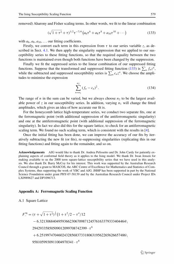
The Ising Susceptibility Scaling Function 579

removed) Aharony and Fisher scaling terms. In other words, we fit to the linear combination

(√

1 + τ 2 + τ)1/2τ−7/4(a6τ

6 + a8τ8 + a10τ

10 + · · · ) (133)

with a6, a8, a10, . . . our fitting coefficients.Firstly, we convert each term in this expression from τ to our series variable z, as de-

scribed in Sect. 4.1. We then apply the singularity suppression that we applied to our sus-ceptibility series to these fitting functions, so that the required equality between the twofunctions is maintained even though both functions have been changed by the suppression.

Finally we fit the suppressed series to the linear combination of our suppressed fittingfunctions. Suppose that the transformed and suppressed fitting function (133) is

∑n fnz

n,while the subtracted and suppressed susceptibility series is

∑n cnz

n. We choose the ampli-tudes to minimise the expression

n2∑

n=n1

(fn − cn)2 . (134)

The range of n in the sum can be varied, but we always choose n2 to be the largest avail-able power of z in our susceptibility series. In addition, varying n1 will change the fittedamplitudes, which gives an idea of how accurate our fit is.

For the honeycomb lattice high-temperature series, we conduct two separate fits, one atthe ferromagnetic point (with additional suppression of the antiferromagnetic singularity)and one at the antiferromagnetic point (with additional suppression of the ferromagneticsingularity). In fact we also did this for the square lattice, to check for an antiferromagneticscaling term. We found no such scaling term, which is consistent with the results in [4].

Once the initial fitting has been done, we can improve the accuracy of our fits by iter-atively subtracting the new fit (or fits), re-suppressing singularities (replicating this in ourfitting functions) and fitting again to the remainder, and so on.

Acknowledgements AJG would like to thank Dr. Andrea Pelissetto and Dr. John Cardy for patiently ex-plaining aspects of conformal field theory as it applies to the Ising model. We thank Dr. Iwan Jensen formaking available to us the 2000 term square-lattice susceptibility series that we have used in this analy-sis. We also thank Dr. Barry McCoy for his interest. This work was supported by the Australian ResearchCouncil through a grant to MASCOS, the ARC Centre of Excellence for Mathematics and Statistics of Com-plex Systems, thus supporting the work of YBC and AJG. JHHP has been supported in part by the NationalScience Foundation under grant PHY-07-58139 and by the Australian Research Council under Project IDsLX0989627 and DP1096713.

Appendix A: Ferromagnetic Scaling Function

A.1 Square Lattice

Fsq− = (τ +

√1 + τ 2)

12(1 + τ 2/2 − τ 4/12

− 6.3213068404959366230670987124576163379333404464\29429335850509012099708742399 · τ 6

+ 6.2519974704602432856837331806319562265626657486\9581059930911004970341 · τ 8

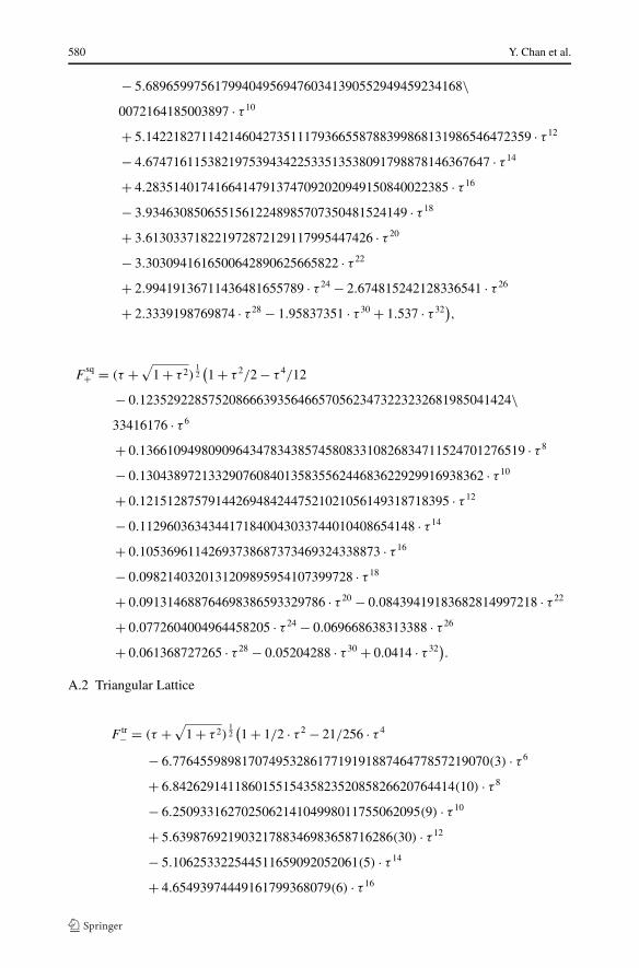
580 Y. Chan et al.

− 5.6896599756179940495694760341390552949459234168\0072164185003897 · τ 10

+ 5.14221827114214604273511179366558788399868131986546472359 · τ 12

− 4.67471611538219753943422533513538091798878146367647 · τ 14

+ 4.28351401741664147913747092020949150840022385 · τ 16

− 3.93463085065515612248985707350481524149 · τ 18

+ 3.613033718221972872129117995447426 · τ 20

− 3.3030941616500642890625665822 · τ 22

+ 2.99419136711436481655789 · τ 24 − 2.674815242128336541 · τ 26

+ 2.3339198769874 · τ 28 − 1.95837351 · τ 30 + 1.537 · τ 32),

Fsq+ = (τ +

√1 + τ 2)

12(1 + τ 2/2 − τ 4/12

− 0.123529228575208666393564665705623473223232681985041424\33416176 · τ 6

+ 0.13661094980909643478343857458083310826834711524701276519 · τ 8

− 0.13043897213329076084013583556244683622929916938362 · τ 10

+ 0.121512875791442694842447521021056149318718395 · τ 12

− 0.1129603634344171840043033744010408654148 · τ 14

+ 0.10536961142693738687373469324338873 · τ 16

− 0.0982140320131209895954107399728 · τ 18

+ 0.091314688764698386593329786 · τ 20 − 0.08439419183682814997218 · τ 22

+ 0.0772604004964458205 · τ 24 − 0.069668638313388 · τ 26

+ 0.061368727265 · τ 28 − 0.05204288 · τ 30 + 0.0414 · τ 32).

A.2 Triangular Lattice

F tr− = (τ +

√1 + τ 2)

12(1 + 1/2 · τ 2 − 21/256 · τ 4

− 6.7764559898170749532861771919188746477857219070(3) · τ 6

+ 6.84262914118601551543582352085826620764414(10) · τ 8

− 6.250933162702506214104998011755062095(9) · τ 10

+ 5.63987692190321788346983658716286(30) · τ 12

− 5.106253322544511659092052061(5) · τ 14

+ 4.65493974449161799368079(6) · τ 16

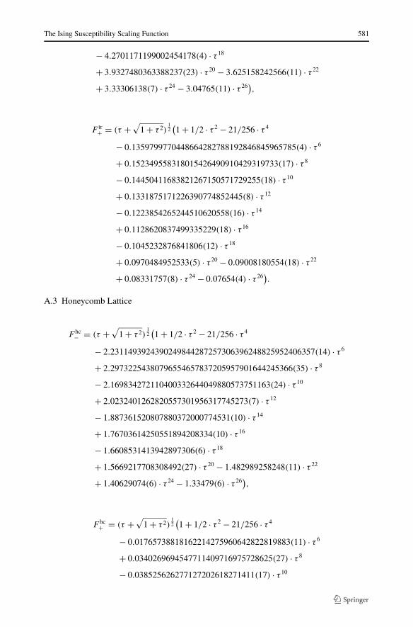
The Ising Susceptibility Scaling Function 581

− 4.2701171199002454178(4) · τ 18

+ 3.9327480363388237(23) · τ 20 − 3.625158242566(11) · τ 22

+ 3.33306138(7) · τ 24 − 3.04765(11) · τ 26),

F tr+ = (τ +

√1 + τ 2)

12(1 + 1/2 · τ 2 − 21/256 · τ 4

− 0.1359799770448664282788192846845965785(4) · τ 6

+ 0.152349558318015426490910429319733(17) · τ 8

− 0.14450411683821267150571729255(18) · τ 10

+ 0.1331875171226390774852445(8) · τ 12

− 0.1223854265244510620558(16) · τ 14

+ 0.1128620837499335229(18) · τ 16

− 0.1045232876841806(12) · τ 18

+ 0.0970484952533(5) · τ 20 − 0.09008180554(18) · τ 22

+ 0.08331757(8) · τ 24 − 0.07654(4) · τ 26).

A.3 Honeycomb Lattice

F hc− = (τ +

√1 + τ 2)

12(1 + 1/2 · τ 2 − 21/256 · τ 4

− 2.2311493924390249844287257306396248825952406357(14) · τ 6

+ 2.29732254380796554657837205957901644245366(35) · τ 8

− 2.169834272110400332644049880573751163(24) · τ 10

+ 2.0232401262820557301956317745273(7) · τ 12

− 1.887361520807880372000774531(10) · τ 14

+ 1.76703614250551894208334(10) · τ 16

− 1.6608531413942897306(6) · τ 18

+ 1.5669217708308492(27) · τ 20 − 1.482989258248(11) · τ 22

+ 1.40629074(6) · τ 24 − 1.33479(6) · τ 26),

F hc+ = (τ +

√1 + τ 2)

12(1 + 1/2 · τ 2 − 21/256 · τ 4

− 0.01765738818162214275960642822819883(11) · τ 6

+ 0.0340269694547711409716975728625(27) · τ 8

− 0.038525626277127202618271411(17) · τ 10

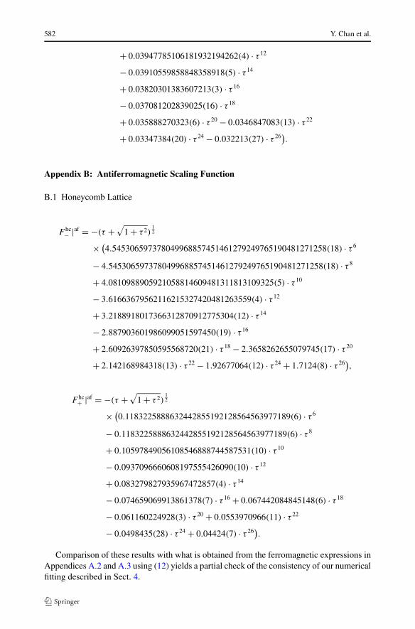
582 Y. Chan et al.

+ 0.03947785106181932194262(4) · τ 12

− 0.03910559858848358918(5) · τ 14

+ 0.03820301383607213(3) · τ 16

− 0.037081202839025(16) · τ 18

+ 0.035888270323(6) · τ 20 − 0.0346847083(13) · τ 22

+ 0.03347384(20) · τ 24 − 0.032213(27) · τ 26).

Appendix B: Antiferromagnetic Scaling Function

B.1 Honeycomb Lattice

F hc− |af = −(τ +

√1 + τ 2)

12

× (4.545306597378049968857451461279249765190481271258(18) · τ 6

− 4.545306597378049968857451461279249765190481271258(18) · τ 8

+ 4.0810988905921058814609481311813109325(5) · τ 10

− 3.61663679562116215327420481263559(4) · τ 12

+ 3.2188918017366312870912775304(12) · τ 14

− 2.887903601986099051597450(19) · τ 16

+ 2.60926397850595568720(21) · τ 18 − 2.3658262655079745(17) · τ 20

+ 2.142168984318(13) · τ 22 − 1.92677064(12) · τ 24 + 1.7124(8) · τ 26),

F hc+ |af = −(τ +

√1 + τ 2)

12

× (0.1183225888632442855192128564563977189(6) · τ 6

− 0.1183225888632442855192128564563977189(6) · τ 8

+ 0.10597849056108546888744587531(10) · τ 10

− 0.0937096660608197555426090(10) · τ 12

+ 0.083279827935967472857(4) · τ 14

− 0.074659069913861378(7) · τ 16 + 0.067442084845148(6) · τ 18

− 0.061160224928(3) · τ 20 + 0.0553970966(11) · τ 22

− 0.0498435(28) · τ 24 + 0.04424(7) · τ 26).

Comparison of these results with what is obtained from the ferromagnetic expressions inAppendices A.2 and A.3 using (12) yields a partial check of the consistency of our numericalfitting described in Sect. 4.

The Ising Susceptibility Scaling Function 583

Appendix C: Short-Distance Terms

Here we give the short-distance “regular” background terms of the form

B =∞∑

q=0

�√q�∑

p=0

b(p,q)(log |τ |)pτ q

rounded to 15 places. Our complete results are available in [43].

C.1 Ferromagnetic Square Lattice

Bsq = (τ +√

1 + τ 2)1/2

× [−.104133245093831 − .074368869753207 τ − .008144713909120 τ 2

+ .004504107712232 τ 3 + .239618794254722 τ 4 − .002539950595339 τ 5

− .235288909669962 τ 6 + .001915707531701 τ 7 + .214340096611538 τ 8

− .000883215706003 τ 9 − .194220628407196 τ 10 + .000007233509777 τ 11

+ .177102037555467 τ 12 + .000688811096268 τ 13 − .162792536489746 τ 14

− .001236572355315 τ 15 + .150013412064378 τ 16 + .001671694059110 τ 17

− .138208109106217 τ 18 − .002022002972782 τ 19 + .126799277310505 τ 20

+ .002308285588780 τ 21 − .115396441906289 τ 22 − .002545765264414 τ 23

+ .103574086263807 τ 24 + .002745532102527 τ 25 − .090922989554413 τ 26

− .002916073299270 τ 27 + .076954225263348 τ 28 + .003063568441388 τ 29

+ (ln |τ |)× (+.032352268477309 τ − .005775529379688 τ 3 + .059074961290345 τ 4

+ .003058491575856 τ 5 − .059166272208841 τ 6 − .002067088393167 τ 7

+ .054246930704214 τ 8 + .001060102531550 τ 9 − .049300253157083 τ 10

− .000268300641612 τ 11 + .045027052571957 τ 12 − .000343326832572 τ 13

− .041428586463053 τ 14 + .000819393297118 τ 15 + .038202673904453 τ 16

− .001196464684146 τ 17 − .035217475800642 τ 18 + .001500680711946 τ 19

+ .032331741680806 τ 20 − .001750700134389 τ 21 − .029449221445927 τ 22

+ .001959866123653 τ 23 + .026464090269923 τ 24 − .002137779981361 τ 25

− .023274239921560 τ 26 + .002291702790868 τ 27 + .019757464449312 τ 28

− .002426942629382 τ 29)

+ (ln |τ |)2

× (+.009391569871146 τ 4 − .008695925462879 τ 6 + .007669481493105 τ 8

584 Y. Chan et al.

+ .000154284382979 τ 9 − .006805407688144 τ 10 − .000310520937481 τ 11

+ .006113866432195 τ 12 + .000444606198236 τ 13 − .005557100215116 τ 14

− .000554418149346 τ 15 + .005078042485427 τ 16 + .000643607994970 τ 17

− .004649202184071 τ 18 − .000716232782651 τ 19 + .004246382079429 τ 20

+ .000775832889819 τ 21 − .003853404958387 τ 22 − .000825213786325 τ 23

+ .003454329481031 τ 24 + .000866512510954 τ 25 − .003034537504706 τ 26

− .000901440561715 τ 27 + .002577451310655 τ 28 + .000931250046525 τ 29)

+ (ln |τ |)3

× (−.000015771569138 τ 9 + .000034428206621 τ 11 − .000052442717749 τ 13

+ .000068823835730 τ 15 − .000002084325090 τ 16 − .000083482363640 τ 17

+ .000006458964601 τ 18 + .000096589603855 τ 19 − .000013639281329 τ 20

− .000108385585447 τ 21 + .000023853448397 τ 22 + .000119105615864 τ 23

− .000037600547029 τ 24 − .000128947973257 τ 25 + .000055460969100 τ 26

+ .000138099034068 τ 27 − .000078321412692 τ 28 − .000146701272364 τ 29)

+(ln |τ |)4

× (−.000000145427323 τ 16 + .000000452982068 τ 18 − .000000959267146 τ 20

+ .000001683186013 τ 22 − .000002660926741 τ 24 − .000000003368087 τ 25

+ .000003934622630 τ 26 + .000000009693809 τ 27 − .000005565949306 τ 28

− .000000023894457 τ 29)

+ (ln |τ |)5

× (+.000000000141953 τ 25 − .000000000441519 τ 27

+ .000000001224727 τ 29)]

.

C.2 Antiferromagnetic Square Lattice

Bafsq = (τ +

√1 + τ 2)1/2

× [+.158866522960947 + .149566836938536 τ + .010712225879833 τ 2

+ .012753018839962 τ 3 − .011741188869656 τ 4 − .014066040875666 τ 5

+ .013106454615626 τ 6 + .012239696625538 τ 7 − .011840194045411 τ 8

− .010585409302312 τ 9 + .010151560037724 τ 10 + .009080004112331 τ 11

− .008542012228790 τ 12 − .007717026940132 τ 13 + .007123677682511 τ 14

+ .006508646391366 τ 15 − .005912245104109 τ 16 − .005467010793273 τ 17

+ .004900133679335 τ 18 + .004597213578999 τ 19 − .004074131287647 τ 20

The Ising Susceptibility Scaling Function 585

− .003893839411793 τ 21 + .003417128190380 τ 22 + .003339548120697 τ 23

− .002905973440848 τ 24 − .002906261172134 τ 25 + .002510579952576 τ 26

+ .002559795034096 τ 27 − .002197017191525 τ 28 − .002268131101616 τ 29

+ (ln |τ |)× (−.155317190158011 τ + .032067148145870 τ 3 − .007716887572462 τ 4

− .015675211573817 τ 5 − .000285542451537 τ 6 + .009607254502732 τ 7

+ .004835406420625 τ 8 − .006064990344481 τ 9 − .007340015041447 τ 10

+ .003910356521404 τ 11 + .008708427445682 τ 12 − .002697783010885 τ 13

− .009405623038077 τ 14 + .002161267525775 τ 15 + .009683424894714 τ 16

− .002106502189570 τ 17 − .009696425760611 τ 18 + .002374179655585 τ 19

+ .009556527066075 τ 20 − .002827702235523 τ 21 − .009355445823856 τ 22

+ .003353500098021 τ 23 + .009167728425385 τ 24 − .003868501274293 τ 25

− .009041887308405 τ 26 + .004329857870148 τ 27 + .008988699114041 τ 28

− .004740651061453 τ 29)

+ (ln |τ |)2

× (+.011533714378823 τ 4 − .011311734920692 τ 6 + .010045768711199 τ 8

− .000475698571097 τ 9 − .008783972022287 τ 10 + .001157180172964 τ 11

+ .007680651109513 τ 12 − .001865091261620 τ 13 − .006744701894515 τ 14

+ .002491836298308 τ 15 + .005964068368078 τ 16 − .002972695839442 τ 17

− .005327647984236 τ 18 + .003273731192324 τ 19 + .004822634345908 τ 20

− .003388237983845 τ 21 − .004425467442049 τ 22 + .003335544654325 τ 23

+ .004094631068058 τ 24 − .003157926493823 τ 25 − .003772517361799 τ 26

+ .002912409430061 τ 27 + .003402363586667 τ 28 − .002655520057041 τ 29)

+ (ln |τ |)3

× (+.000057899719476 τ 9 − .000169915088240 τ 11 + .000326648846875 τ 13

− .000517190858645 τ 15 − .000001422188017 τ 16 + .000729027463661 τ 17

+ .000009170599968 τ 18 − .000948102082432 τ 19 − .000032108584334 τ 20

+ .001159641637018 τ 21 + .000080604994072 τ 22 − .001349862803424 τ 23

− .000160502424863 τ 24 + .001508463556122 τ 25 + .000264448046627 τ 26

− .001631439353298 τ 27 − .000364294406680 τ 28 + .001722930696448 τ 29)

+ (ln |τ |)4

× (−.000000160856746 τ 16 + .000000456983407 τ 18 − .000000040918655 τ 20

586 Y. Chan et al.

− .000003417322708 τ 22 + .000013997416073 τ 24 − .000000009021984 τ 25

− .000036813182410 τ 26 + .000000125169178 τ 27 + .000075735555538 τ 28

− .000000779435552 τ 29)

+ (ln |τ |)5

× (−.000000001286222 τ 25 + .000000004385050 τ 27

+ .000000027799861 τ 29)]

.

C.3 Ferromagnetic Triangular Lattice

Btr = (τ +√

1 + τ 2)1/2

× [−.049561116521763 − .029358763163227 τ − .003802085786368 τ 2

+ .006390376143904 τ 3 + .194331491416170 τ 4 − .004659659320547 τ 5

− .195488838278358 τ 6 + .003651173504528 τ 7 + .178621656686715 τ 8

− .002895748949957 τ 9 − .161336242614720 τ 10 + .002311455809247 τ 11

+ .146284971711630 τ 12 − .001842503338574 τ 13 − .133577942096403 τ 14

+ .001456977882233 τ 15 + .122753362974429 τ 16 − .001134805649081 τ 17

− .113263489337451 τ 18 + .000862240813452 τ 19 + .104601807098273 τ 20

− .000629270080307 τ 21 − .096359884476827 τ 22 + .000428320304385 τ 23

+ (ln |τ |)× (−.005374288589598 τ + .001021325616916 τ 3 + .049253501657254 τ 4

− .000006005387528 τ 5 − .050675128993180 τ 6 − .000277768605459 τ 7

+ .046680337431830 τ 8 + .000300252836069 τ 9 − .042334826787302 τ 10

− .000227268452048 τ 11 + .038476859060257 τ 12 + .000114673447726 τ 13

− .035187926212720 τ 14 + .000011949942590 τ 15 + .032370727904288 τ 16

− .000140047340708 τ 17 − .029894415736149 τ 18 + .000263535279625 τ 19

+ .027634040948919 τ 20 − .000379722086737 τ 21 − .025487516010638 τ 22

+ .000487692500440 τ 23)

+ (ln |τ |)2

× (+.008301571737990 τ 4 − .007863822472801 τ 6 + .006940825976817 τ 8

+ .000004920887586 τ 9 − .006124967722414 τ 10 − .000008028657674 τ 11

+ .005459215424842 τ 12 + .000010897860945 τ 13 − .004918734820641 τ 14

− .000014290481783 τ 15 + .004471830270400 τ 16 + .000018331038938 τ 17

− .004090720207698 τ 18 − .000022918919968 τ 19 + .003752754837032 τ 20

The Ising Susceptibility Scaling Function 587

+ .000027921194209 τ 21 − .003440642618124 τ 22 − .000033228452894 τ 23)

+ (ln |τ |)3

× (−.000008243826432 τ 9 + .000019339918959 τ 11 − .000030791103742 τ 13

+ .000041558105858 τ 15 − .000000289107374 τ 16 − .000051264920936 τ 17

+ .000001306093325 τ 18 + .000059839322918 τ 19 − .000003538519413 τ 20

− .000067344361243 τ 21 + .000007394079439 τ 22 + .000073895527830 τ 23)

+ (ln |τ |)4

× (−.000000023041822 τ 16 + .000000103665399 τ 18 − .000000280140679 τ 20

+ .000000584762202 τ 22)]

.

The leading term in Btr above confirms the estimate in (26) of [20] after adding a factor 2needed because of a difference in conventions.

C.4 Ferromagnetic Honeycomb Lattice

Bhc = (τ +√

1 + τ 2)1/2

× [−.221526277068482 − .170518806873542 τ − .019236029093417 τ 2

− .000240258087320 τ 3 + .140112831065240 τ 4 + .002715126912573 τ 5

− .139853710977321 τ 6 − .002422123613147 τ 7 + .130966255841349 τ 8

+ .002478441994620 τ 9 − .121767984156181 τ 10 − .002593394970413 τ 11

+ .113507041635338 τ 12 + .002697199234761 τ 13 − .106296857456039 τ 14

− .002778848577189 τ 15 + .099986481192228 τ 16 + .002840749390802 τ 17

− .094433287150951 τ 18 − .002887196461298 τ 19 + .089489266542983 τ 20

+ .002921915790808 τ 21 − .084984336381365 τ 22 − .002947776518703 τ 23

+ (ln |τ |)× (+.110304596706594 τ − .017367191250168 τ 3 + .032554394731493 τ 4

+ .007749610093406 τ 5 − .033370773266168 τ 6 − .004545306065368 τ 7

+ .031517394252347 τ 8 + .002697183732340 τ 9 − .029438657077664 τ 10

− .001512880972029 τ 11 + .027527821013048 τ 12 + .000704802950233 τ 13

− .025841562449391 τ 14 − .000126907282155 τ 15 + .024355378143637 τ 16

− .000302184134792 τ 17 − .023041033316250 τ 18 + .000630617459438 τ 19

+ .021866143676416 τ 20 − .000888340903130 τ 21 − .020791271125817 τ 22

+ .001094822052575 τ 23)

+ (ln |τ |)2

588 Y. Chan et al.

× (+.004328421950579 τ 4 − .004173174221495 τ 6 + .003864856815018 τ 8

+ .000098594831882 τ 9 − .003581293629898 τ 10 − .000203109598421 τ 11

+ .003336710555165 τ 12 + .000293321457772 τ 13 − .003126961910309 τ 14

− .000367344803112 τ 15 + .002944831872355 τ 16 + .000427433155150 τ 17

− .002785081058367 τ 18 − .000476286169756 τ 19 + .002642924163304 τ 20

+ .000516221811618 τ 21 − .002513107496440 τ 22 − .000549081268363 τ 23)

+ (ln |τ |)3

× (−.000008459084030 τ 9 + .000018328291997 τ 11 − .000027731894823 τ 13

+ .000036311733546 τ 15 − .000000100196269 τ 16 − .000044084313016 τ 17

+ .000000291941736 τ 18 + .000051136242275 τ 19 − .000000616104491 τ 20

− .000057556878974 τ 21 + .000001226160802 τ 22 + .000063427686583 τ 23)

+ (ln |τ |)4

× (−.000000008316207 τ 16 + .000000024195538 τ 18 − .000000049128873 τ 20

+ .000000092415863 τ 22)]

.

C.5 Antiferromagnetic Honeycomb Lattice

Bafhc = (τ +

√1 + τ 2)1/2

[.122404044024957 + .111801280547087 τ + · · ·

+ (ln |τ |)(−.121053173885789 τ + · · · ) + · · · ],as given more fully by (13) and Appendices C.3 and C.4.

References

1. Domb, C.: Order-disorder statistics. II. A two-dimensional model. Proc. R. Soc. Lond. A 199, 199–221(1949)

2. Domb, C., Green, M.S. (eds.) Series Expansions for Lattice Models. Phase Transitions and CriticalPhenomena, vol. 3. Academic Press, London (1974)

3. Orrick, W.P., Nickel, B.G., Guttmann, A.J., Perk, J.H.H.: Critical behavior of the two-dimensional Isingsusceptibility. Phys. Rev. Lett. 86, 4120–4123 (2001). arXiv:cond-mat/0009059

4. Orrick, W.P., Nickel, B., Guttmann, A.J., Perk, J.H.H.: The susceptibility of the square lattice Isingmodel: new developments. J. Stat. Phys. 102, 795–841 (2001). arXiv:cond-mat/0103074. For the com-plete set of series coefficients, see http://www.ms.unimelb.edu.au/~tonyg

5. Nickel, B.: On the singularity structure of the 2D Ising model susceptibility. J. Phys. A, Math. Gen. 32,3889–3906 (1999)

6. Wu, T.T., McCoy, B.M., Tracy, C.A., Barouch, E.: Spin-spin correlation functions for the two dimen-sional Ising model: exact theory in the scaling region. Phys. Rev. B 13, 315–374 (1976)

7. Barouch, E., McCoy, B.M., Wu, T.T.: Zero-field susceptibility of the two-dimensional Ising modelnear Tc . Phys. Rev. Lett. 31, 1409–1411 (1973)

8. Tracy, C.A., McCoy, B.M.: Neutron scattering and the correlation functions of the two-dimensional Isingmodel near Tc . Phys. Rev. Lett. 31, 1500–1504 (1973)

9. Jimbo, M., Miwa, T.: Studies on holonomic quantum fields. XVII. Proc. Jpn. Acad. A 56, 405–410(1980). Errata: Proc. Japan Acad. A 57, 347 (1981)

The Ising Susceptibility Scaling Function 589

10. Au-Yang, H., Perk, J.H.H.: Correlation functions and susceptibility in the Z-invariant Ising model. In:Kashiwara, M., Miwa, T. (eds.) MathPhys Odyssey 2001: Integrable Models and Beyond, pp. 23–48.Birkhäuser, Boston (2002). Preprint at http://physics.okstate.edu/perk/papers/kyoto/ziising.pdf

11. Guttmann, A.J.: Susceptibility amplitudes for the two-dimensional Ising model. Phys. Rev. B 9, 4991–4992 (1974). Errata: Phys. Rev. B 12, 1991 (1975)

12. Ritchie, D.S., Betts, D.D.: Extended universality of the Ising model. Phys. Rev. B 11, 2559–2563 (1975)13. Au-Yang, H., Perk, J.H.H.: Susceptibility calculations in periodic and quasiperiodic planar Ising models.

Physica A 321, 81–89 (2003)14. Kong, X.P.: Wave vector dependent susceptibility of the two dimensional Ising model. Ph.D. Thesis,

State University of New York at Stony Brook (1987)15. Fisher, M.E.: Transformations of Ising models. Phys. Rev. 113, 969–981 (1959)16. Aharony, A., Fisher, M.E.: Nonlinear scaling fields and corrections to scaling near criticality. Phys. Rev.

B 27, 4394–4400 (1983)17. Aharony, A., Fisher, M.E.: Universality in analytic corrections to scaling for planar Ising models. Phys.

Rev. Lett. 45, 679–682 (1980)18. Guttmann, A.J.: Ising model amplitudes and extended lattice-lattice scaling. J. Phys. A, Math. Gen. 10,

1911–1916 (1977)19. Gaunt, D.S., Guttmann, A.J.: A generalised form of extended lattice-lattice scaling. J. Phys. A, Math.

Gen. 11, 1381–1397 (1978)20. Mangazeev, V.V., Dudalev, M.Yu., Bazhanov, V.V., Batchelor, M.T.: Scaling and universality in the two-

dimensional Ising model with a magnetic field. Phys. Rev. E 81, 060103(R) (2010). arXiv:1002.423421. Caselle, M., Hasenbusch, M., Pelissetto, A., Vicari, E.: Irrelevant operators in the two-dimensional Ising

model. J. Phys. A, Math. Theor. 35, 4861–4888 (2002). arXiv:cond-mat/010637222. Gradshteyn, I.S., Ryzhik, I.M.: Table of Integrals, Series, and Products, 4th edn. Academic Press, New

York (1980)23. Syozi, I.: Transformation of Ising Models. In: Domb, C., Green, M.S. (eds.) Exact Results. Phase Tran-

sitions and Critical Phenomena, vol. 1. Academic Press, London (1972)24. Perk, J.H.H.: Quadratic identities for Ising model correlations. Phys. Lett. A 79, 3–5 (1980)25. McCoy, B.M., Wu, T.T.: Nonlinear partial difference equations for the two-dimensional Ising model.

Phys. Rev. Lett. 45, 675–678 (1980)26. McCoy, B.M., Wu, T.T.: Nonlinear partial difference equations for the two-spin correlation function of

the two-dimensional Ising model. Nucl. Phys. B 180[FS2], 89–115 (1980)27. McCoy, B.M., Perk, J.H.H., Wu, T.T.: Ising field theory: quadratic difference equations for the n-point

Green’s functions on the square lattice. Phys. Rev. Lett. 46, 757–760 (1981)28. McCoy, B.M., Wu, T.T.: The Two-Dimensional Ising Model. Harvard University Press, Cambridge

(1973)29. Baxter, R.J.: Solvable eight-vertex model on an arbitrary planar lattice. Philos. Trans. R. Soc. Lond. A

289, 315–346 (1978)30. Au-Yang, H., Perk, J.H.H.: Critical correlations in a Z-invariant inhomogeneous Ising model. Physica A

144, 44–104 (1987)31. Au-Yang, H., Perk, J.H.H.: Wavevector-dependent susceptibility in aperiodic planar Ising models. In:

Kashiwara, M., Miwa, T. (eds.) MathPhys Odyssey 2001: Integrable Models and Beyond, pp. 1–21.Birkhäuser, Boston (2002). Preprint at http://physics.okstate.edu/perk/papers/kyoto/triquasi.pdf

32. Naya, S.: On the spontaneous magnetizations of honeycomb and kagomé Ising lattices. Prog. Theor.Phys. 11, 53–62 (1954)

33. Witte, N.S.: Isomonodromic deformation theory and the next-to-diagonal correlations of the anisotropicsquare lattice Ising model. J. Phys. A, Math. Theor. 40, F491–F501 (2007). arXiv:0705.0557

34. Houtappel, R.M.F.: Order-disorder in hexagonal lattices. Physica 16, 425–455 (1950)35. Wannier, G.H.: Antiferromagnetism. The triangular Ising net. Phys. Rev. 79, 357–364 (1950). Errata:

Phys. Rev. B 7, 5017 (1973)36. Newell, G.F.: Crystal statistics of a two-dimensional triangular Ising lattice. Phys. Rev. 79, 876–882

(1950)37. Hancock, H.: Lectures on the Theory of Elliptic Functions, arts. 251, 357–360. Dover Publications,

New York (1958)38. Whittaker, E.T., Watson, G.N.: A Course of Modern Analysis, 4th edn. Cambridge University Press,

Cambridge (1927). Chaps. 21 and 2239. Stephenson, J.: Ising model spin correlations on the triangular lattice. J. Math. Phys. 5, 1009–1024

(1964)40. Sykes, M.F., Gaunt, D.S., Martin, J.L., Mattingly, S.R., Essam, J.W.: Derivation of low-temperature ex-

pansions for Ising model. IV. Two-dimensional lattices: temperature grouping. J. Math. Phys. 14, 1071–1074 (1973)

590 Y. Chan et al.

41. Sykes, M.F., Gaunt, D.S., Roberts, P.D., Wyles, J.A.: High temperature series for the susceptibility of theIsing model. I. Two dimensional lattices. J. Phys. A 5, 624–639 (1972)

42. Sykes, M.F., Watts, M.G., Gaunt, D.S.: Derivation of low-temperature expansions for Ising model. VIII.Ferromagnetic and antiferromagnetic polynomials for the honeycomb-triangular system. J. Phys. A,Math. Gen. 8, 1448–1460 (1975)

43. Chan, Y., Guttmann, A.J., Nickel, B.G., Perk, J.H.H.: Additional material added to the source files ofarXiv:1012.5272

44. Boukraa, S., Guttmann, A.J., Hassani, S., Jensen, I., Maillard, J.-M., Nickel, B., Zenine, N.: Experimentalmathematics on the magnetic susceptibility of the square lattice Ising model. J. Phys. A, Math. Theor.41, 455202 (2008). arXiv:0808.0763. See http://www.ms.unimelb.edu.au/~iwan/ising/Ising_ser.html forthe series coefficients

45. Nickel, B.: Addendum to ‘On the singularity structure of the 2D Ising model susceptibility’. J. Phys. A,Math. Gen. 33, 1693–1711 (2000)

46. Vaidya, H.G.: The spin-spin correlation functions and susceptibility amplitudes for the two-dimensionalIsing model: triangular lattice. Phys. Lett. A 57, 1–4 (1976)

47. Matveev, V., Shrock, R.: Complex-temperature singularities in the d = 2 Ising model: triangularand honeycomb lattices. J. Phys. A, Math. Gen. 29, 803–823 (1996). arXiv:hep-lat/9411023 andarXiv:hep-lat/9412076