Embed Size (px)
Citation preview
THE IONOSPHERIC Z RAY RETURN MECHANISM
by
'J.l.. \~>I' v.j\. .
t>'il' c.l J.W.Hudspeth,B.Sc.(Hons.)
submitted in fulfilment
of the·requirements for the degree of
Doctor of Philosophy
UNIVERSITY OF TASMANIA
HOBART
MARCH 1982 lc,r..,·,_ ¥- r~- eJ ~V\cvr c.l,.. l q ~ 3
This thesis contains no material which
has been accepted for the award of any
other degree or diploma in any university.
To the best of my knowledge and belief,
the thesis contains no copy or paraphrase of
material preTiously published or written by
another person, except where due reference
is made in the text.
ACKNOWLEDGEMENTS
SUMMARY
CHAPTER 1: INTRODUCTION
CONTENTS
•
CHAPTER 2: BACKGROUND THEORY • •
2.1 Introduction
2.2 The Appleton-Hartree Formula
2.3 The Booker Quartic Equation
•
2.4 Poeverlein's Graphical Construction
CHAPTER 3: REVIEW OF Z MODE THEORY •
~ ..
12
13
19
29
3.1 Introduction 34
3.2 Z Mode Generation Mechanism 34
3.3 Return Of The Z Ray - Backscatter 42
3.4 Critical Discussion 47
3.5 Return Of The Z Ray - Bowman 57
3.6 Critical Discussion 66
3.7 Return Of The Z Ray - Papagiannis 75
3.8 Critical Discussion 79
3.9 Return Of The Z Ray - Papagiannis And Miller 92
3.10 Critical Discussion 101
3.11 Ray Tracing 114
3.12 Summary And Proposals For Experimental Tests 120
CHAPTER 4: OBSERVATIONAL TECHNIQUE
4.1 Introduction 127
4.2 The Instruments 128
7
• 12
• 34
.127
4.3 Observing Programme
4o4 Analysis
CHAPTER FIVEg RESULTS
5.1 Angle Of Arrival - Z Echoes
5o2 Angle Of Arrival - 0 And X Echoes
5.3 Scattering Patterns On h'f Ionograms
5.4 Fast Runs
5.5 Z Splitting
CHAPTER 6: DISCUSSION ;
6.1 Introduction
6.2 Solar Zenith Angle Tilt Theory
603 ~ackscatter Theory
6 .4 Tilt Theory
6.5 Conclusions
CHAPTER 7: THE Z DUCT RETURN MECHANISM
? .1 Introduction
7.2 The Z Duct Model
7o3 Computer Ray Tracing
7.4 Ionospheric Ducts
7.5 Z Splitting
7.6 Discussion
7.7 Direct Evidence
CHAPTER 8: CONCLUSIONS
8.1 Summary
8.2 Recommendations For Future Research
SELECTED BIBLIOGRAPHY
134
135
140
142
161
161
175
176
176
177
177
179
181
181
184
196
201
203
210
213
214
217
• 140
• 176
181
.213

ACKNOWLEDGEMENTS
This research was conducted over several years, part time
and without financial assistance. I therefore thank not only
the many people who assisted in various ways with the research
work but also those assisting with part time and temporary full
time employment.
In particular I thank the following people and
organisations
- my supervisor Prof.G.R.A.Ellis for encouragement, for
stimulating discussions and for critical evaluation of
my work.
- Mr.G.T.Goldstone, OIC of the Hobart Ionospheric Station,
for assistance with electronics, logistics, ionospheric
records and scaling.
- the staff and students of the Physics Dept. (especially
Mr.B.T.Wilson).
- the University Computing Centre 0 the University Library,
the University Photographic and Printing Sections.
- the Ionospheric Prediction Service (especially
Dr.L.McNamara).
- my friends, my parents 9 my wife's parents and especially
my wife for their willing support.
SUfJMARY
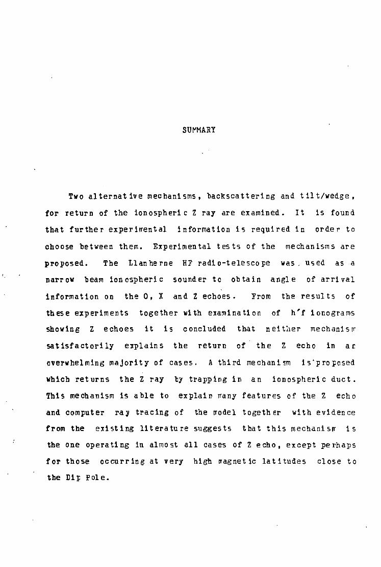
Two alternative mechanisms, backscattering and tilt/wedge,
for return of the ion osph eri c Z ray are examined. It is found
that further experirrental information is required in order to
choose between them. Experimental tests of the mechanisms are
proposed. The Llanherne HF radio-telescope was. used as a
narrow beam ionospheric sounder to obtain angle of arrival
information on the 0, X and Z echoes. From the results of
these experiments together with examination of h'f ionograms
showing Z echoes it is concluded that neiti.1er mechanisrr
satisfactorily e::xplains the return of the Z echo in ar.
overwhelming majority of cases. A tbird mechani~m is'pro:pased
which returns the Z ray by trapping in an ionospheric duct.
This mechanism is able to explain ~any features of the Z echo
and computer ra1 tracing of the rrodel together with evidence
from the existing literature suggests that this mechanisrr is
the one operating in almost all cases of Z echo, except perhaps
for those occurring at very high rragnetic latitudes close to
t be Di i: P ol e •
7
CHAPTER ONE
INTRODUCTION
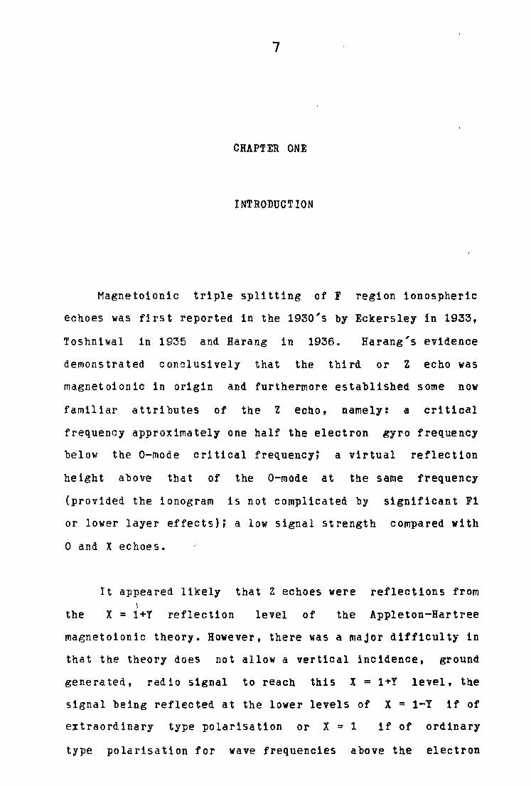
Magnetoionic triple splitting of F region ionospheric
echoes was first reported in the 1930's by Eckersley in 1933,
Toshniwal in 1935 and Harang in 1936. Harang's evidence
demonstrated conclusively that the third or Z echo was
magnetoionic in origin and furthermore established some now
familiar attributes of the Z echo, namely: a critical
frequency approximately one half the electron gyro frequency
below the 0-mode critical frequency; a virtual reflection
height above that of the 0-mode at the same frequency
(provided the ionogram is not complicated by significant Fl
or lower layer effects); a low signal strength compared with
0 and X echoes.
It appeared likely that Z echoes were reflections from \
the X = 1+Y reflection level of the Appleton-Hartree
magnetoionic theory. However, there was a major difficulty in
that the theory does not allow a vertical incidence, ground
generated, radio signal to reach this X = l+Y level, the
signal being reflected at the lower levels of X = 1-Y if of
extraordinary type polarisation or X = 1 if of ordinary
type polarisation for wave frequencies above the electron
gyro frequency.
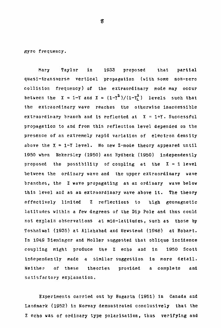
Mary Taylor in 1933 proposed that partial
quasi-transverse vertical propagation (with some non-zero
collision frequency) of the extraordinary mode may occur
between the a 2 x = 1-Y and x = (1-Y )/(1-YL) levels such that
the extraordinary wave reaches the otherwise inaccessible
extraordinary branch and is reflected at X = l+Y. Successful
propagation to and from this reflection level depended on the
presence of an extremely rapid variation of electron density
above the X = 1-Y level. No new Z-mode theory appeared until
1950 when Eckersley (1950) ann Rydbeck (1950) independently
proposed the possibility of coupling at the X = 1 level
between the ordinary wave and the upper extraordinary wave
branches, the Z wave propagating as an ordinary wave below
this level and as an extraordinary wave above it. The theory
effectively limited Z reflections to high geomagnetic
latitudes within a few degrees of the Dip Pole and thus could
not explain observations at mid-latitudes, such as those by
Toshniwal (1935) at Allahabad and Newstead (1948) at Hobart.
In 1949 Dieminger and Moller suggested that oblique incidence
coupling might produce tne Z echo and in 1950 Scott
independently made a similar suggestion in more detail.
Neither of these theories provided a complete and
satisfactory explanation.
Experiments carried out by Hogarth (1951) in Canada and
Landmark (1952) in Norway demonstrated conclusively that the
Z echo was of ordinary type polarisation, thus verifying and
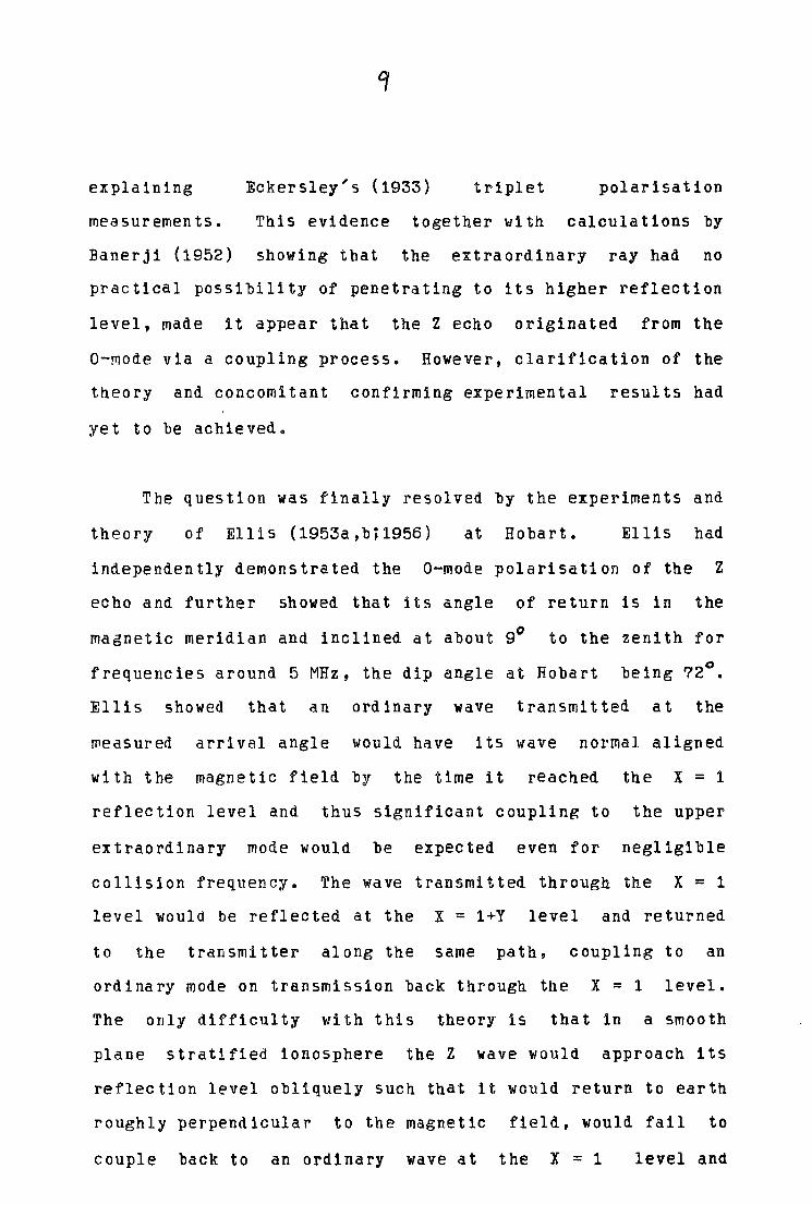
explaining
measurements.
Eckersley's (1933) triplet polarisation
This evidence together with calculations by
Banerji (1952) showing that the extraordinary ray had no
practical possibility of penetrating to its higher reflection
level, made it appear that the Z echo originated from the
0-mode via a coupling process. However, clarification of the
tneory and concomitant confirming experimental results had
yet to be achieved.
The question was finally resolved by the experiments and
theory of El 1 is (1953a,b;1956) at Hobart. Ellis had
independently demonstrated the 0-mode polarisation of the z
echo and further showed that its angle of return is in the
magnetic meridian and inclined at about gO to the zenith for
frequencies around 5 MHz, the dip angle at Hobart being 72°.
Ellis showed that an ordinary wave transmitted at the
measured arrival angle would have its wave normal aligned
with the magnetic field by the time it reached the X = 1
reflection level and thus significant coupling to the upper
extraordinary mode would be expected even for negligible
collision frequency. The wave transmitted through the X = 1
level would be reflected at the X = l+Y level and returned
to the transmitter along the same path, coupling to an
ordinary mode on transmission back through the X = 1 level.
The only difficulty with this theory is that in a smooth
plane stratified ionosphere the Z wave would approach its
reflection level obliquely such that it would return to eartn
roughly perpendicular to the magnetic field, would fail to
couple back to an ordinary wave at the X = 1 level and
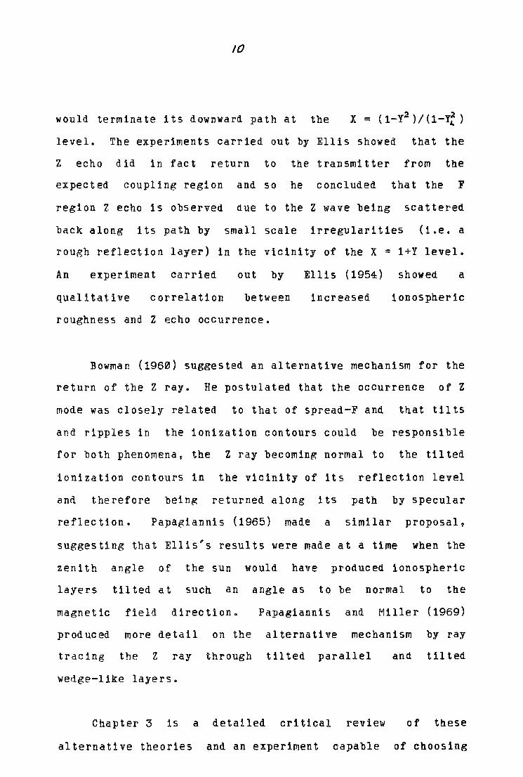
10
would terminate its downward path at the X = ( 1-Y2 ) I ( 1 -Y~ )
level. The experiments carried out by Ellis showed that the
Z echo did in fact return to the transmitter from the
expected coupling region and so he concluded that the F
region Z echo is observed due to the Z wave being scattered
back along its path by small scale irregularities (i.e. a
rough reflection layer) in the vicinity of the X = l+Y level.
An experiment carried out by Ellis (1954) showed a
qualitative correlation between increased ionospheric
roughness and Z echo occurrence.
Bowman (1960) suggested an alternative mechanism for the
return of the Z ray. He postulated that the occurrence of Z
mode was closely related to that of spread-F and that tilts
and ripples in the ionization contours could be responsible
for both phenomena, the Z ray becoming normal to the tilted
ionization contours in the vicinity of its reflection level
and therefore bein~ returned along its path by specular
reflection. Papagiannis (1965) made a similar proposal,
suggesting that Ellis's results were made at a time when the
zenith angle of the sun would have produced ionospheric
layers tilted at such an angle as to be normal to the
magnetic field direction. Papagiannis and Miller (1969)
produced more detail on the
tracing the Z ray through
wedge-like layers.
alternative mechanism
tilted parallel and
by ray
tilted
Chapter 3 is a detailed critical review of these
alternative theories and an experiment capable of choosing
II
between them is proposed. The following chapters give an
account of an investigation carried out to determine the
mechanism(s) appropriate to the return of the Z ray.
Chapter 2 provides a brief description of background theory
relevant to the problem.
2.1 Introduction
12.
CHAPTER TWO
BACKGROUND THEORY
The following sections comprise brief descriptions of the
Appleton-Hartree formula, the Booker quartic equation and the
graphical method of Poeverlein. The content of these sections
is mainly draw~ directly from the works of Ratcliffe (1962) and
Budden (1961,1964) and the original papers by
B~oker (1936,1938) and Poeverlein (1948,1949,1950). No attempt
is made to describe the general features of the magnetoionic
theory or wave propagation in the ionosphere and formulae are I I
quoted without derivation. Interested readers are referred to
the treatises by Ratcliffe and Budden.
The following notation has been adopted and is employed
throughout this and the subsequent chapters.
c = free space velocity of electromagnetic waves
e = charge on electron (when numerical values are inserted
this will be negative)
H0 = magnitude of the imposed Magnetic field
k = angular wave number (=2rr/~)
m = mass of electron
n = complex refractive index (;tt-iX)
N = number density of electrons
13
W = angular wave frequency
jJ- = refractive index (=real part of n)
X = absorption coefficient
X = Kc/w = absorption index = negative imaginary part of n
~0 = magnetic permittivity of free space
€0 = electric permittivity of free space
e = angle the wave normal makes with the vertical (z direct
-ion)
9 = angle the wave normal k makes with the magnetic field H
V = frequency of collisions of electrons with heavy
particles
(.JH = j'oHo I e I /m
X = W02 /1,,J2.
Y = <.Jn/ <.J
z = V/W
U = 1-iZ
YT='( £in 9
Y,_ = Y cos®
!. = j<o~e/mW 11 ,m 1 ,n1 = direction cosines of vector Y (anti-parallel to H0 -
since e is negative)
2.2 The Appleton-Hartr~e Formula
The refractive index of a medium containing free
14-
electrons, with a superimposed steady magnetic field is given
by
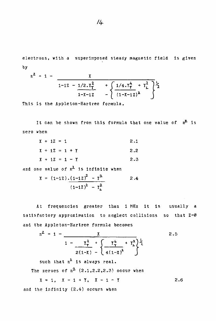
n2. = 1 - x
1-iZ - 1/2.Yi
1-X-iZ {
4. + 1/4.YT +
- (1-X-1Z)2.
This is the Appleton-Hartree formula.
y'- 2 2 }~
It can be shown from this formula that one value of n~ is
zero when
x + iZ = 1 2.1
x + iZ = 1 + y 2.2
x + iZ = 1 - y 2.3
and one value of nl. is infinite when
x = ( 1 - i z ) . ( 1 - i z )2. - y1- 2.4
(1-iZ)1 - yl. ,_
At frequencies greater than 1 MHz it is usually a
satisfactory approxi~ation to neglect collisions so that Z=0
and the Appleton-Hartree formula becomes
nz. = 1 -
1 - y2 T
2 ( 1-X)
x
such that n1 is always real.
The zeroes of n~ (2.1,2.2,2.3) occur when
X = 1, X = 1 + Y, X = 1 - Y
and the infinity (2.4) occurs when
2.5
2.6

x = 1 - Y2
1 - Yf
15
2.7
Furthermore, when X=l, one of the values of n2 is unity.
The F-region gyro frequency at Hobart is about 1.4 MHz at
ionospheric heights and as radio sounding of the Hobart F-layer
rarely drops below this frequency we shall consider only the
case for Y < 1. For a medium such as the ionosphere, the
generally most useful way to consider refractive index )
variation is to plot curves showing the dependence/of na upon
X, Y being relatively constant at a given location. If the
wave normal is parallel or anti-parallel to the earth's
magnetic field, Y = 0 and we have purely longitudinal
propagation, the variation of n4 with X being shown in Fig.2.1.
If the wave normal is perpendicular to the earth's magnetic
field, Y = 0 and we have purely transverse propagation as
shown in Fig.2.2. The variation of n2 with X for the case when
the angle between the earth's magnetic field and the ·wave
normal is intermediate between the purely transverse and purely
longitudinal cases is shown by the shaded regions of Fig.2.3,
the thick lines representing typical curves. The dotted lines
show the limiting positions for purely transverse and purely
longitudinal propagation and together with the line X = 1 form
the boundaries within which t~e curves for an intermediate case
must always lie. For the intermediate case n2 has an infinity
w~en X is given by 2.7 and this infinity lies between 1-Yi and
1 •
:?IG.2.1
~IG.2.2
"F TG • 2 .3
Variation of n' with X for purely longitudinal propagation, when Y < I •
. r 1l2
r n2
Variation of n1 with X for purely transverse propagation when Y < 1.
-1
.·:·.-.... . . · ···:):·:· .... , .. , ....
··· ....
Vari3tion of 11• with X for intenncdi,11c inclin.ition of the 1·arth's magnetic field, when Y <I. Electron colh~ion~ a1c ncglcct(;d.
( F iG' s • t: . 1 t o 6 • 3 o f Bu d rl e r , 1 ~; ( i 1 )
17
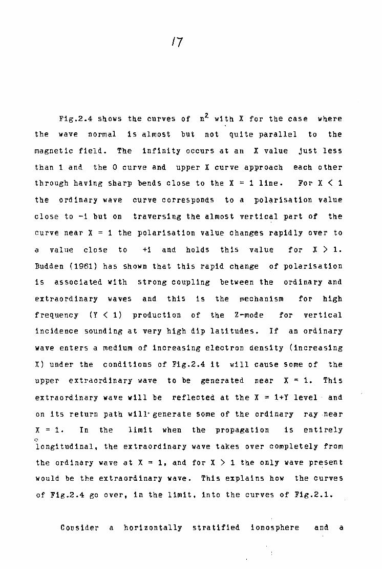
Fig.2.4 shows the curves of nz with X for the case where
the wave normal is almost but not quite parallel to the
magnetic field. The infinity occurs at an X value just less
than 1 and the O curve and upper X curve approach each other
through having sharp bends close to the X = 1 line. For X < 1
the ordinary wave curve corresponds to a polarisation value
close to -i but on traversing the almost vertical part of the
curve near X = 1 the polarisation value changes rapidly over to
a value close to +1 and holds this value for X > 1.
Budden (1961) has shown that this rapid change of polarisation
is associated with strong coupling between the ordinary and
extraordinary waves and this is the mechanism for high
frequency (Y < 1) production of the Z-mode for vertical
incidence sounding at very high dip latitudes. If an ordinary
wave enters a medium of increasing electron density (increasing
X) under the conditions of Fig.2.4 it will cause some of the
upper extraordinary wave to be generated near X = 1. This
extraordinary wave will be reflected at the X = l+Y level · and
on its return path will• generate some of the ordinary ray near
x = 1. In the limit when the propagation is entirely Q
longitudinal, the extraordinary wave takes over completely from
the ordinary wave at X = 1, and for X > 1 the only wave pr~sent
would be the extraordinary wave. This explains how the curves
of Fig.2.4 go over, in the limit, into the curves of Fig.2.1.
Consider a horizontally stratified ionosphere and a
18
linearly polarised radiowave normally incident from below. As
the ionosphere is a birefringent medium, there will be two
transmitted waves and the quantities which refer to them will
be distinguished by subscripts a and b respectively. The two
waves will have polarisations ptA. and fb and
n~ and nb given by the Appleton-Hartree
refractive indices
formula. Since the
wave normal of the incident wave is initially vertical,
Snell's law shows that the wave normals of both the ordinary
and extrordinary waves in the ionosphere are, and remain,
normal (though this is not generally true of the ray
direction). It is therefore possible to determine the
propagation paths of the waves through the layers and to
calculate the reflection and transmission coefficients at each
boundary.
However the case for oblique incidence raises some
difficulties. Consider a plane wave incident upon the
ionosphere from below with its wave normal at an angle 81 to
the vertical and let for the two transmitted waves the
refractive indices be n~ and nb and the wave normal angles to
the vertical be f)o.- and l}~ respectively. As Snell's law applies
for both waves
2.8
If n~ and nb were known then the unknown angles 6~ and ~b could
be determined but the values of n~ and nb depend upon YL, Y;
which in turn depend upon 9~ and gb • Equation 2.8 therefore
cannot be used directly to find e~ and ob and herein lies the
1q
problem of determining propagation paths at oblique incidence.
The Booker quartic equation, as described in the following
section, is normally used to overcome this obstacle.
2.3 The Booker Quartic Equation
Consider again a wave incident upon the ionosphere from
below and consider one transmitted component only, as the
following applies equally to both. As before, from Snell's law
sin&? = n.sin e where n and e are both unknown but n.sin9 is known and we may
define the quantity q, first introduced into magnetoionic
theory by Booker (1936,1939), as
q = n.cos9
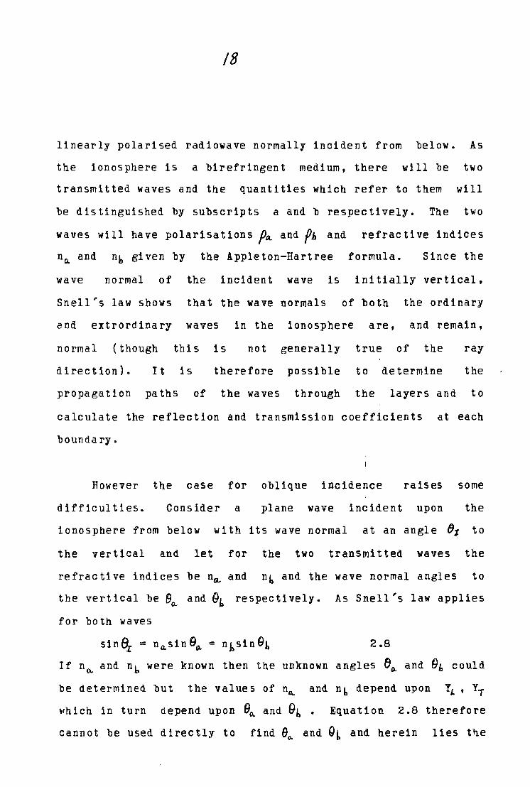
If we treat the refractive index n as though it were a vector
inclined at an angle e to the vertical then q is its v~rtical
component and sinB1 its horizontal component (Fig.2.5). If q
is known, n and e follow from the relations
nz = q2 + siniel tanG = sinS1 /q
q is the root of the quartic equation known as the Booker
quartic. The following argument is a more general case which
reduces to the preceding argument when S2=0.
Consider a wave incident obliquely from below upon a
horizontally stratified, slowly varying ionosphere sue~ that in
free space below the plasma its wave normal has direction
1
( :F ii;. f. .1- of Jud den, 1S61)
' " ' ' ' ... ' ...
' ' ' '\ ' '
FIG.2.4
" ' \ ·~, • , - L '
I ( _;', J'~. '. 1
''' ~~- -.
' ,·,· ,' r ' ~ ' . :' '
Variation of n1 with X when the propagation is almost longitudinal and Y < 1.
FIG.2.5
(Fig.E.11 of J:udden, 1 S61)
I .....: ......... ,
...... ' ' ...
q
sin fJ 1
Relation between the refract!\ e index n, the variable q, and the angle 0 bet\\ een che wave-normal and the vertical.
' \ \
\ \
' o~~~~~~~·r~\'--~~~~4R~~-+N
o i.-------N-'r'~,-------:c*'----N :A\ I
I I ,
1NA NB I
I
FIG.2.6
\
' ' \ ' ' \
' ' q2 as a function of N, ycrtical
incidence. FIG. 2.? q as a function of N, vertical
incidence.
O' i gs . 5 a r: d 6 o f B o o k e r , 1 g cB )
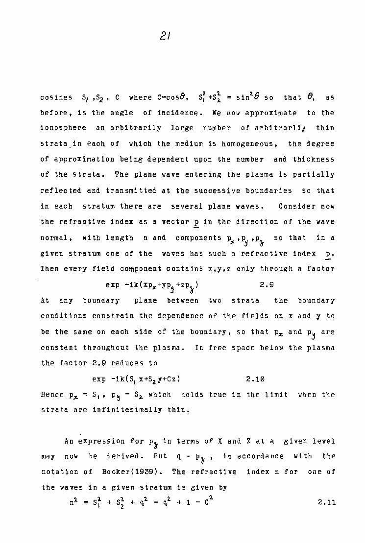
21
cosines s1 ,s2 , C where C=cosfJ, that e, as
before, is the angle of incidence. We now approximate to the
ionosphere an arbitrarily large number of arbitrarliy thin
strata in each of which the medium is homogeneous, the degree
of approximation being dependent upon the number and thickness
of the strata. The plane wave entering the plasma is partially
reflected and transmitted at the successive boundaries so that
in each stratum there are several plane waves. Consider now
the refractive index as a vector p in the direction of the wave
normal, with length n and components p ,p ,p~ :1- :J 0
so that in a
given stratum one of the waves has such a refractive index p.
Then every field component contains x,y,z only through a factor
2.9
At any boundary plane between two strata the boundary
conditions constrain the dependence of the fields on x and y to
be the same on each side of the boundary, so that p~ and pj are
constant throughout the plasma. In free space below the plasma
the factor 2.9 reduces to
2.10
Hence P;ir. = S1 , p~ = S2. which tlolds true in the limit when the
strata are infinitesimally thin.
An expression for p) in terms of X and Z at a given level
may now be derived. Put in accordance with the
notation of Booker(1939). The refractive index n for one of
the waves in a given stratum is given by
n'- = s~ + s~ + q1 == q1 + 1 - c'2. 2.11
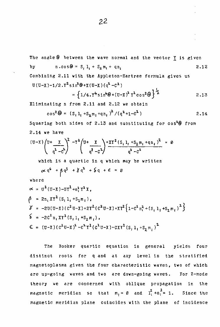
22
The angle 9 bet ween the wave normal and the vector Y is given
by
Combining 2.11 with the Appleton-Hartree formula gives us
u ( u -x ) -1I2 • Y 2 s i n1 9 + x ( u -x ) ( q2 -c 2 )
= { 1/4. y't-sin4B + (U-X )2 y2 co sa®} \
Eliminating n from 2.11 and 2.12 we obtain
cos2 ® = ( S1 11 +S 4 m1 +qn1 )2 /(q2 +1-C1)
Squaring both sides of 2.13 and substituting for cos1 9 from
2.14 we have
(U-X)(U+ 2-\2 -Y
1(U+ ~ \+XY 2 (s, 1, +S2m1 +qn, )
1 = 0
q1 -c1.} q1 -c 4/ qi -c1
which is a quartic in q which may be written
()I.. q" + r q3 + ~ q2. + ~ q + € = 0
where
~ = u 1 (U-X)-UY2 +n~Y1 X,
~ = 2n 1 XY 2 (S 1 11 +S1m1),
"I= -2U(U-X)(C2 U-X)+2Y2.(C2 U-X)+XY2 {1-c2 n~+(s, l,+s2m1 )1
}
~ = -2Cin. XY 2 (s, 1, +S2 m I),
£ = (U-X)(C1 U-X)1 -C').Y1 (C1.U-X)-CXY2 (s,1,+s2.ml )2
2.12
2.13
2.14
The Booker quartic equation in general yields four
distinct roots for q and at any level in the stratified
magnetoplasma gives the four characteristic waves, two of which
are up-going waves and two are down-going waves. For Z-mode
theory we are concerned with oblique propagation in the
magnetic meridian so that m = 0 and I Since the
magnetic meridian plane coincides with the plane of incidence
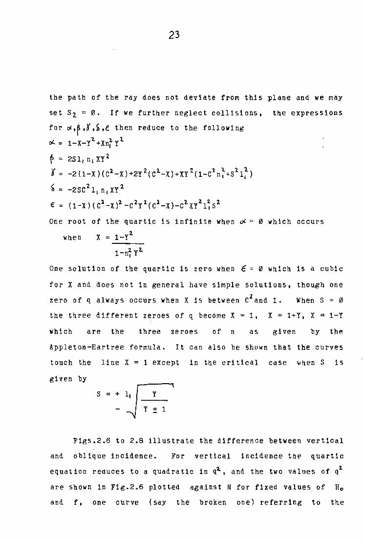
23
the path of the ray does not deviate from this plane and we may
set Sz = 0. If we further neglect collisions, the expressions
for ~,r,r,~,e then reduce to the following 'l. 'l. l.
ol.. = 1-X-Y +Xn1 Y
~ = 2S 1 1 n 1 XY 2
'f = -2(1-X)(c2 -X)+2Y 2 (c 1-X)+XY 2 (1-c1n;+s
11;)
t' 2 2 <1 = -2SC 1 1 n 1 XY
€ = (1-X) ( c 1 -X)1 -C 2 Y 1 (c 2 -X)-C1 XY1 1~ s2
One root of the quartic is infinite when o< = 0 which occurs
when X = 1-Y1
1-n2 Y2. I
One solution of the quartic is zero when e = 0 wh.ich is a cubic
for X and does not in general have simple solutions, though one 2 zero of q always occurs when X is between C and 1. When S = 0
the three different zeroes of q become X = 1, X = l+Y, X = 1-Y
which are the three zeroes of n as given by the
Appleton-Hartree formula. It can also be shown that the curves
touch the line X = 1 except in the critical case when S is
given by
s = + 11 y
y + 1
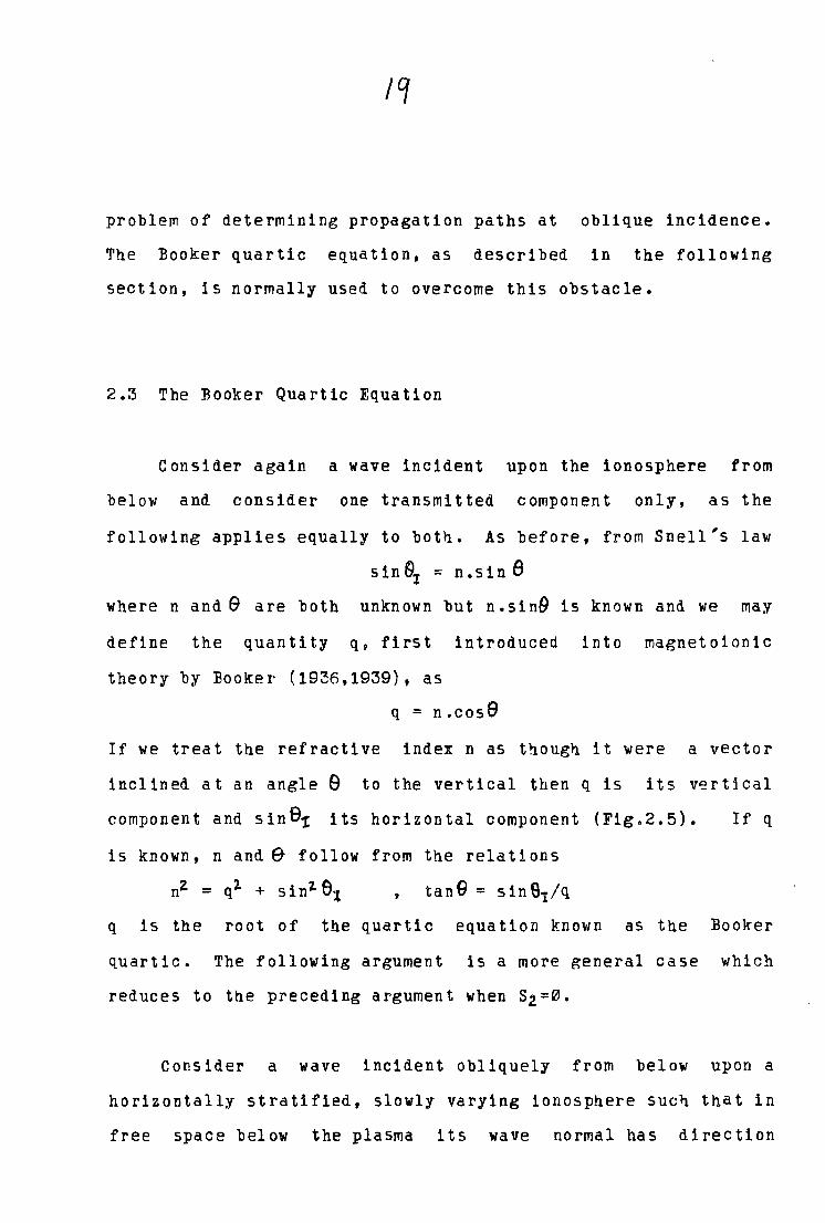
Figs.2.6 to 2.8 illustrate the difference between vertical
and oblique incidence. For vertical incidence the quartic
equation reduces to a quadratic in q'2., and the two values of q'1.
are shown in Fig.2.6 plotted against N for fixed values of H0
and f, one curve (say the broken one) referring to the
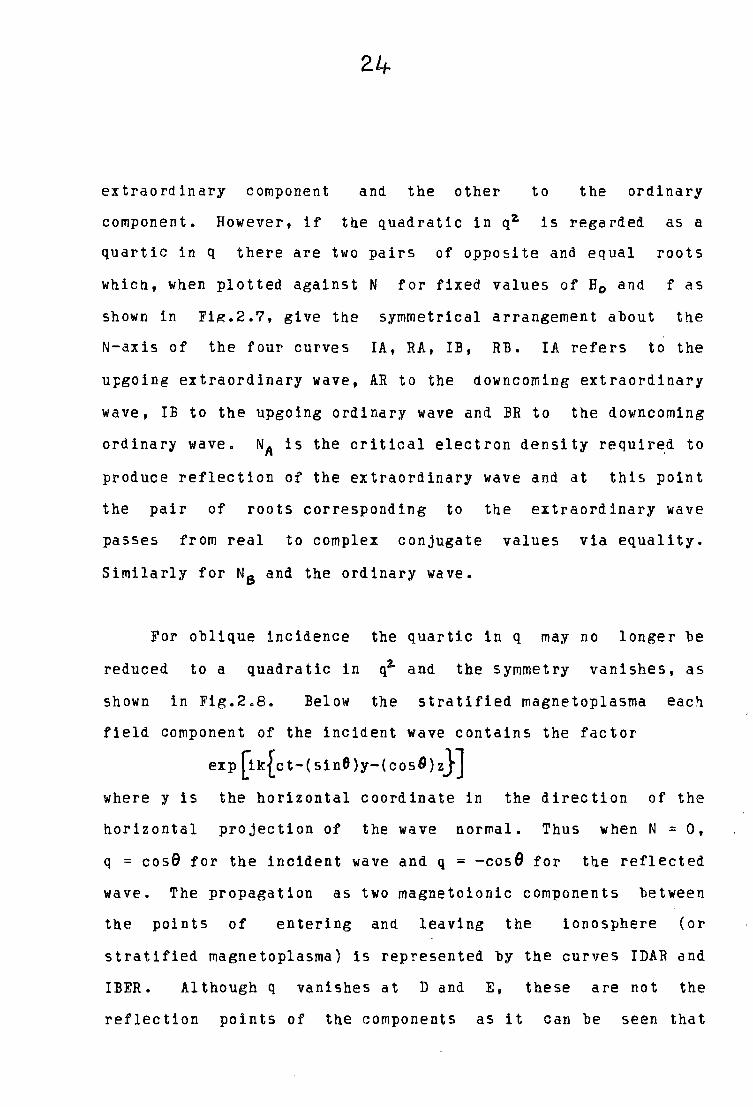
24
extraordinary component and the other to the ordinary
component. However, if the quadratic in q2 is regarded as a
quartic in q there are two pairs of opposite and equal roots
which, when plotted against N for fixed values of H0 and f as
shown in Fig.2.7, give the symmetrical arrangement about the
N-axis of the four curves IA, RA, IB, RB. IA refers to the
upgoing extraordinary wave, AR to the downcoming extraordinary
wave, IB to the upgoing ordinary wave and BR to the downcorning
ordinary wave. NA is the critical electron density requir~d to
produce reflection of the extraordinary wave and at this point
the pair of roots corresponding to the extraordinary wave
passes from real to complex conjugate values via equality.
Similarly for N8 and the ordinary wave.
For oblique incidence the quartic in q may no longer be
reduced to a quadratic in q~ and the symmetry vanishes, as
shown in Fig.2.8. Below the stratified magnetoplasma each
field component of the incident wave contains the factor
exp[ik{ct-(sin6)y-(cos9)z}]
where y is the horizontal coordinate in the direction of the
horizontal projection of the wave normal. Thus when N = 0,
q = case for the incident wave and q = -case for the reflected
wave. The propagation as two magnetoionic components between
the points of entering and leaving the ionosphere (or
stratified magnetoplasma) is represented by the curves !DAR and
!BER. Although q vanishes at D and E, these are not the
reflection points of the components as it can be seen that
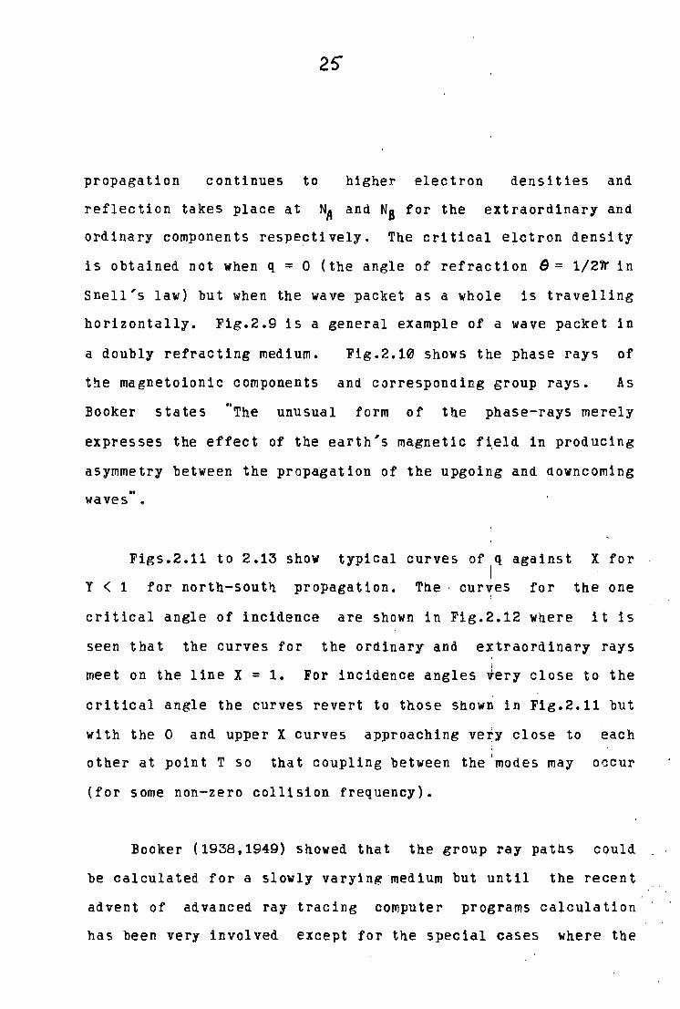
2~
propagation continues to higher electron densities and
reflection takes place at NA and N8 for the extraordinary and
ordinary components respectively. The critical elctron density '
is obtained not when q = 0 (the angle of refraction B = 1/2~ in
Snell's law) but when the wave packet as a whole is travelling
horizontally. Fig.2.9 is a general example of :a wave packet in
a doubly refracting medium. Fig.2.10 shows the phase rays of
the magnetoionic components and corresponding group rays. As
Booker states " The unusual form of tne phase-rays merely
expresses the effect of the earth's magnetic field in producing
asymmetry between the propagation of the upgoing and aowncoming
" waves •
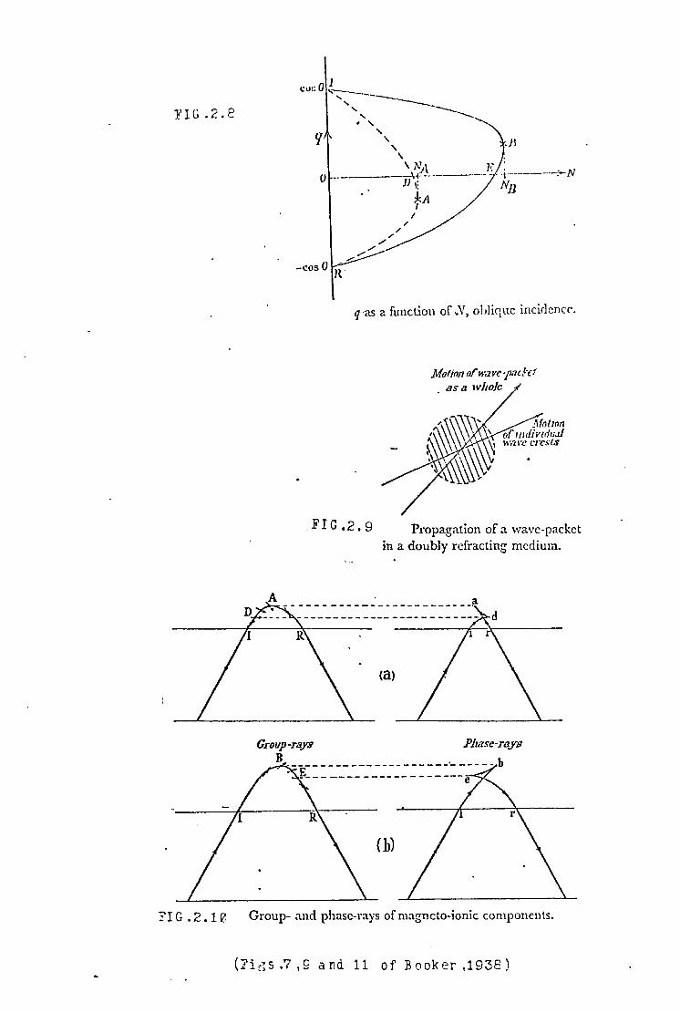
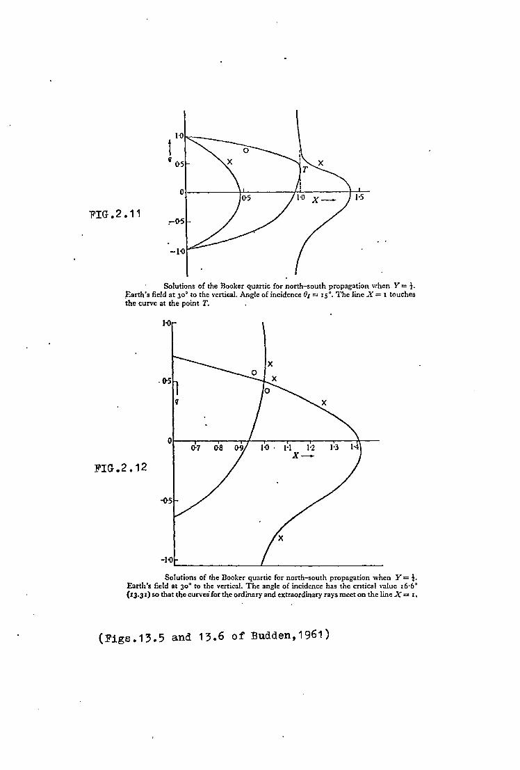
Figs.2.11 to 2.13 show typical curves of q against X for I
I Y < 1 for north-south propagation. Tne curves for the one
'
critical angle of incidence are shown in Fig.2.12 where it is
seen that the curves for the ordinary and extraordinary rays I
meet on the line X = 1. For incidence angles very close to the
critical angle the curves revert to those shown in Fig.2.11 but
with the 0 and upper X curves approaching ve~y close to each
other at point T so that coupling between the 'modes may occur
(for some non-zero collision frequency).
Booker (1938,1949) showed that the group ray paths could
be calculated for a slowly varying·medium but until the recent
advent of advanced ray tracing computer programs calculation
has been very involved except for the special cases where the
}'I G • 2. e
?IG.2.10
.•.. 0 1 cl .. , ____ _
' --'l '
''' ----------' ' ' ' ' .)3
\ 1'}\ ll ------------\~- ------
]) ,:
-cos 0 n.·
~A I
q ·as a function of .• V, oblique incidcnc<".
Motion t}Jw,zve-p.uh:t as a whole :<
- FIG • 2. 9 Propagation of a wave-packet
in a doubly refracting medium.
A - - - - - - - - - - - - - - - - - - - - - - - - _;:i.
Group-rli.)'9 Pl1ase-rays B
---------------------~-----b - E ____________________ e
(h)
Group- and phase-rays of magneto-ionic components.
( 7 i t; s • 7 , S a n d 11 o f B o o k er , 19 3 B )
1-0
t " 0-5
0 1-5
'FIG. 2. 11 :-0-5
Solutions of the Booker quartic for north-south propagation when Y = t. ,Earth's field at 30° to the vertical. Angle of incidence 01=15°. The line X = I touches the curve at the point T.
1-0
x . 0-5
"
(}7 0-8 1-0 . 1"l 1·2 x-
FIG.2 .12
-0-5
-1-0
Solutions of the Booker quartic for north-south propagation when Y = !. Earth's field at 30° to the vertical. The angle of incidence has the critical value 16·6° (13.31) so that the curves-for the ordinary and extraordinary rays meet on the line X = 1.
(Figs.13.5 and 13.6 of Budden,1961)
l·O
X-1·5
FIG.2.13 x
-1-0
· Solutions of the Booker quartic for north-south propagation when Y = !. Earth's field at 30' to the vertical. Angle of mcidcnce 01 = 45°. The right branch of the cur\'e for the extraordinary wa\'e touches the !me X = 1 at the point T as shown in the inset diagram with an expanded scale of X,
;;; ~ 'U t: <&: ti u
'O ·::i
c:: it 0 ~
J e
FIG.2 .14
Cross-section of refractive index surface by a plane containing the direction of the earth's magnetic field. CX and CA are the normal and tangent, respectively, at the point C. CB is perpendicular to OC.
(Figs.13.7 and 13.19 of Budden,1961)
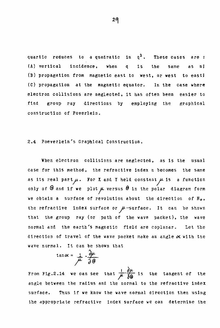
quartic reduces to a quadratic in q1 • These cases are :
(A) vertical incidence, when q is the same as n;
{B) propagation from magnetic east to west, or west to east;
(C) propagation at the magnetic equator. In the case where
electron collisions are neglected, it has often been easier to
find group ray directions by employing the graphical
construction of Poverlein.
2.4 Poeverlein's Graphical Construction.
When electron collisions are neglected, as is the usual
case for this method, the refractive index n becomes the same
as its real part.I'.
only of 8 and if we
For X and Y held constant~ is a function
plot,t-- versus 8 in the polar diagram form
we obtain a surface of revolution about the direction of Ha,
the refractive
that the group
index surface or /-surface.
ray {or path of the wave
It can be shown
packet), the wave
normal and the earth's magnetic field are coplanar. Let the
direction of travel of the wave packet make an angle()( with t~e
wave normal. It can be shown that
tan O< = .-1. • ...?e:.-f d@
From Fig.2.14 we can see that ~·ii is the tangent of the
angle between the radius and the normal to the refractive index
surface. Thus if we know the wave normal direction then using
the appropriate refractive index surface we can determine the
30
group ray direction by constructing the normal to that surface
at the point at which its radius vector is the wave normal
direction.
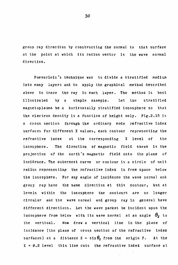
Poeverlein's technique was to divide a stratified medium
into many layers and to apply the graphical method described
above to trace the ray in each layer. The method is best
illustrated by a simple example. Let the stratified
magnetoplasma be a horizontally stratified ionosphere so that
the electron density is a function of height only. Fig.2.15 is
a cross section through the ordinary mode refractive index
surfaces for different X values, each contour representin~ the
refractive index at the corresponding X level of the
ionosphere. The direction of magnetic field shown is the
projection of the earth's magnetic field onto the plane of
incidence. The outermost curve or contour is a circle of unit
radius representing the refractive index in free space below
the ionosphere. For any angle of incidence the wave normal and
group ray have the same direction at this contour, but at
levels within the ionosphere the contours are no longer
circular and the wave normal and group ray in general have
different directions. Let the wave packet be incident upon the
ionosphere from below with its wave normal at an angle 8z to
the vertical. Now draw a vertical line in the plane of
incidence (the plane of cross section of the refractive index
surfaces) at a distance S = sin6r from the origin P. At the
X = 0.2 level this line cuts the refractive index surface at
OIAECTION OF /'1AGN£nc t VE.f{TICAL
FIELD
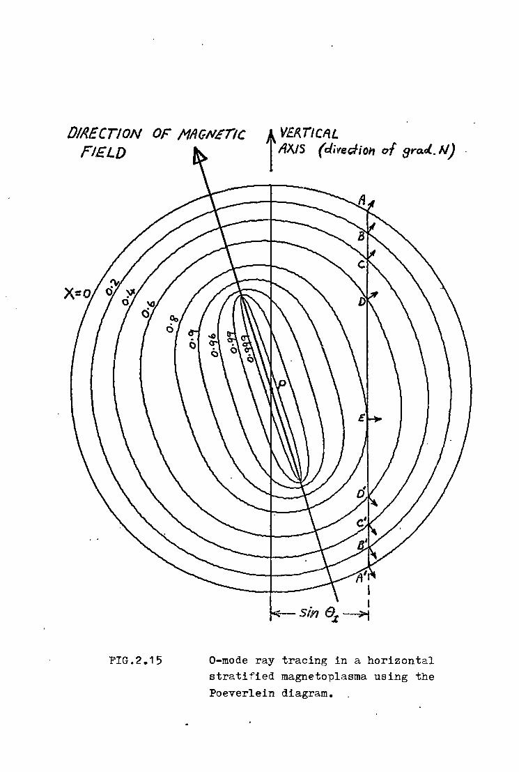
FIG.2.15
AXIS (d.i.,ediotr of 9ra.J.. N)
0-mode ray tracing in a horizontal stratified magnetoplasma using the
Poeverlein diagram.
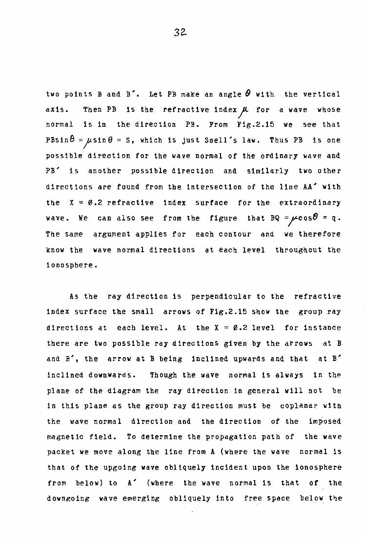
two points Band B'. Let PB make an angle B with the vertical
axis.
normal
Then PB
is in
is the refractive index~ for
the direction PB. From Fig.2.15
a wave whose
we see that
PBsin8 =~sine= s, which is just Snell's law. Thus PB is one
possible direction for the wave normal of the ordinary wave and
PB' is another possible direction and similarly two other
directions are found from the intersection of the line AA' with
the X = 0.2 refractive index surface for the extraordinary
wave. We can also see from the figure that BQ =~cos8 = q.
The same argument applies for each contour and we therefore
know the wave normal directions at each level throughout the
ionosphere.
As the ray direction is perpendicular to the refractive
index surface the small arrows of Fig.2.15 show the group ~ay
directions at each level. At the X = 0.2 level for instance
there are two possible ray directions given by the arrows ·at B
and B', the arrow at B being inclined upwards and that at B'
inclined downwards. Though the wave normal is always in the
plane of the diagram the ray direction in general will not be
in this plane as the group ray direction must be coplanar with
the wave normal direction and the direction of the imposed
magnetic field. To determine the propagation path of the wave
packet we move along the line from A (where the wave normal is
that of the upgoing wave obliquely incident upon the ionosphere
from below) to A' (where the wave normal is that of the
downRoing wave emerging obliquely into free space below the

33
ionosphere). The successive intersections
A,B,C,D,E,D',c',B',A' with the refractive index surfaces give
the successive directions of propagation in the appropriate
layers. The more refractive index surfaces utilised
(corresponding to thinner and more numerous strata) tne better
the approximation to the actual propagation path. Energy
propagates upwards through the ionosphere until the point E is
reached where the the line AA' is tangential to the refractive
index surface and here the group ray is horizontal and thus
reflection occurs. Along the line AA' beyond E the wave packet
is propagated downwards through the ionosphere. It should be
noted that a plot of the wave and group ray directions from
this diagram will lead to exactly the same result for the
ordinary wave as that shown in Fig.2.10(b) and using
Poeverlein's construction for tne extraordinary ray leads to
the same result as Fig.2.10(a).
3.1 Introduction
CHAPTER THREE
REVIEW OF Z MODE THEORY
Section 3.2 describes the accepted Z mode generation
mechanism in terms of the original explanation. Sections 3.3,
3.5, 3.7 and 3.9 detail various proposals for the mechanism
responsible for the return of the Z ray. Following directly
after each of these sections is a section of critical
Section 3.12 discussion of the material just presented.
summarises the conclusions drawn throughout the chapter.
3.2 Z Mode Generation Mechanism
Ellis (1953a) reported that measurements of angle of
arrival of Z echoes made at Hobart (dip 72°) on a frequency of
4.65 MHz gave a mean direction of 7.8° north of vertical in the
magnetic plane. In all cases the height of reflection of the Z
echoes was between 170 km and 210 km. Ellis noted that
according to the Quasi-longitudinal hypothesis of Z mode
(e.g.Scott,1950) a collision frequency of about 1.5 x 10~ per
second would be required to explain the observed angle, this
being inconsistent with previous estimates which put the
collision frequency at about 10~ per second at 200 km.
According to Scott the Z mode at a place of dip 72°
(e.g.Hobart) would be caused by quasi-longitudinal propagation
of the 0 mode in a narrow cone around the magnetic field
direction (i.e. 18° north of vertical in the magnetic
meridian), the width of the cone increasing with increasing
collision frequency. For a non-vertical magnetic field Scott
postulated that the Z mode would be seen when the ionosphere
was sufficiently rough to return the Z echo to the transmitter
- in Hobart's case an ionospheric reflecting cone of half angle 0 around 18 would be required.
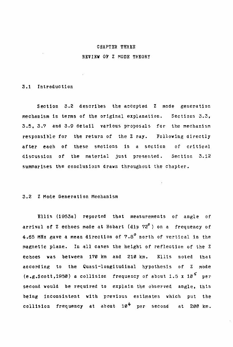
In the same year Ellis (1953b) published further
experimental details and the following explanation for Z mode
generation. For vertical incidence the transition from
transverse to longitudinal propagation ~ay be illustrated by
refractive index curves for different values of ® . The curves
for vertical magnetic field and very high dip magnetic field
are given by the curves of Figs.2.1 and 2.4. The transition
may be described in terms of the change in the shape of the
curves near the X = 1 line, as shown in Fig.3.1. Ellis (1953b)
pointed out that in the Z region there is no qualitative
difference between the transverse extraordinary mode and the
lon~itudinal ordinary mode.
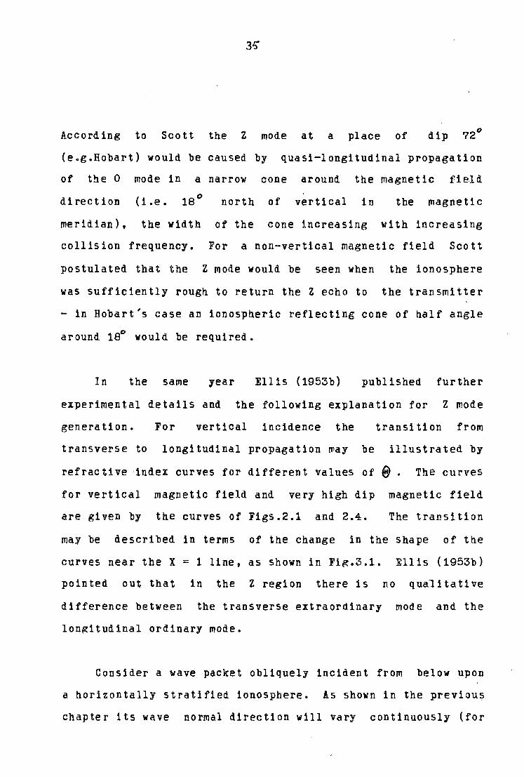
Consider a wave packet obliquely incident from below upon
a horizontally stratified ionosphere. As shown in the previou~
chapter its wave normal direction will vary continuously (for
infinitesimally thick strata) as it propagates upwards through
the ionosphere. For the critical angle of incidence (see
Fig.3.2) the wave normal becomes parallel to the magnetic field
at the ordinary reflection level and penetration of this level
may occur for zero collision frequency. The penetrating wave
propagates on upwards to the Z reflection level.
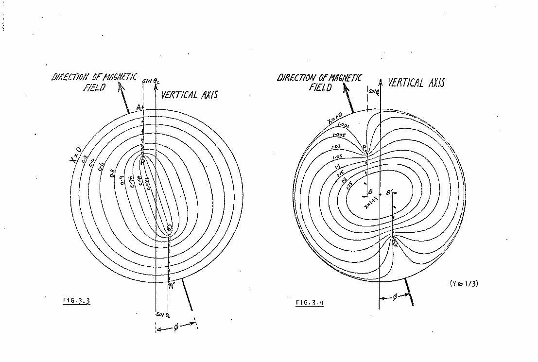
We shall now illustrate the wave propagation by means of
Poerverlein constructions. Fig.3.3 is a polar diagram of the
ordinary mode refractive index curves for the various electron
densities shown (as X values). Fig.3.4 is a polar diagram for
the upper extraordinary mode. The dip angle is 72° and the
wave frequency such that f = 3fH (f would be about 4.3 MHz for
Hobart). For an angle of incidence of 61 we draw the vertical
line a distance sin91 from the diagram origin. The common
value of the refractive index for X = 1, @ = 0 is denoted by P
and that f or X = 1 , 8 = 180 by Q • P and Q are the coupling
points. We choose our line so that it passes through P in
order that the incident wave reaches this coupling point. We
may then graphically determine Be, the necessary critical value
of 9i. Alternatively, since the angle of refraction of the
wave normal 9 at any level in a plane stratified magnetoplasma
is given by Snell's law
sin 9x = n.sin9
and the magnitude of the refractive index for
V = 0 is given by
9 = 0, x = 1,
FIG. 3 .1
(Fig.2 of Ellis,1953)
FIG.3.2
RefrMtivei index ClllTf'S nt the critienl n11g!P. ,,f inc.idcn<;o.
(Fig.1 of Ellis,1956)
~ ;
~ ;;; G ·~ ~ s ~ ~ +·
"" J
" FIG.3.5 q
J J I/ s 6' .?
Frel/11ency --~ M c/s
C1·itit•t1! nugl<'s of i11eitlf'1~l'O fut· Z 1<'fk,•t ion.
(Fig.5 of Ellis,1953)
/J/lf£{770i/ ~F HACllETIC S!ll9c.
11£LO ~ I !. t 1 VEl<TICAL AXIS
\
I ti,~\ l~'J' I I
OIRECT/011 OF 11AGNETIC FIELD VERTICAL AXIS
ISJ,_,4 I
(Y~ 1/3)
FIG.3.4
y
1 + y ' then sin ec = ~sin ¢ -y~
where¢ is the angle the earth's magnetic field makes with the
vertical.
The ordinary wave propagates upwards as showri by
traversing the line AP (Fig.3.3} from A to Po At the coupling
point P conversion to extraordinary mode takes place and we
transfer to point Pon the extraordinary diagram (Fig.3.4).
The wave is now a Z mode wave and continues upwards as
represented by traversing the line from P to B. B represents
the Z reflection point and as we require the wave to couple
again at the X = 1 level and return to the transmitter it is
necess~ry that it be reflected backwards along its incident
path. We therefore jump from point B to point B', this jump
representin~ reversal of both the wave normal and group ray
directions. Traversing the line from B' to Q represents the
reflected Z mode wave travelling back down its path to the
couplin.g point Q at the X = 1 level. Since the upward and
downward propagation paths are identically located in physical
space then P and Q are representative of the same physical
point in the ionosphere. The extraordinary wave at Q couples
back to an ordinary wave which propagates downwards to the
transmitter as represented by the Q to A' line of Fig.3.3.
Ellis (195E} noted that Poeverlein (1949} and Millington (1954)
had also pointed out the possibility of mode conversion at the
X = 1 level giving rise to the upper extraordinary mode at
oblique incidence.
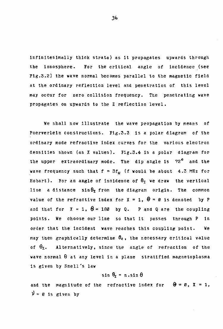
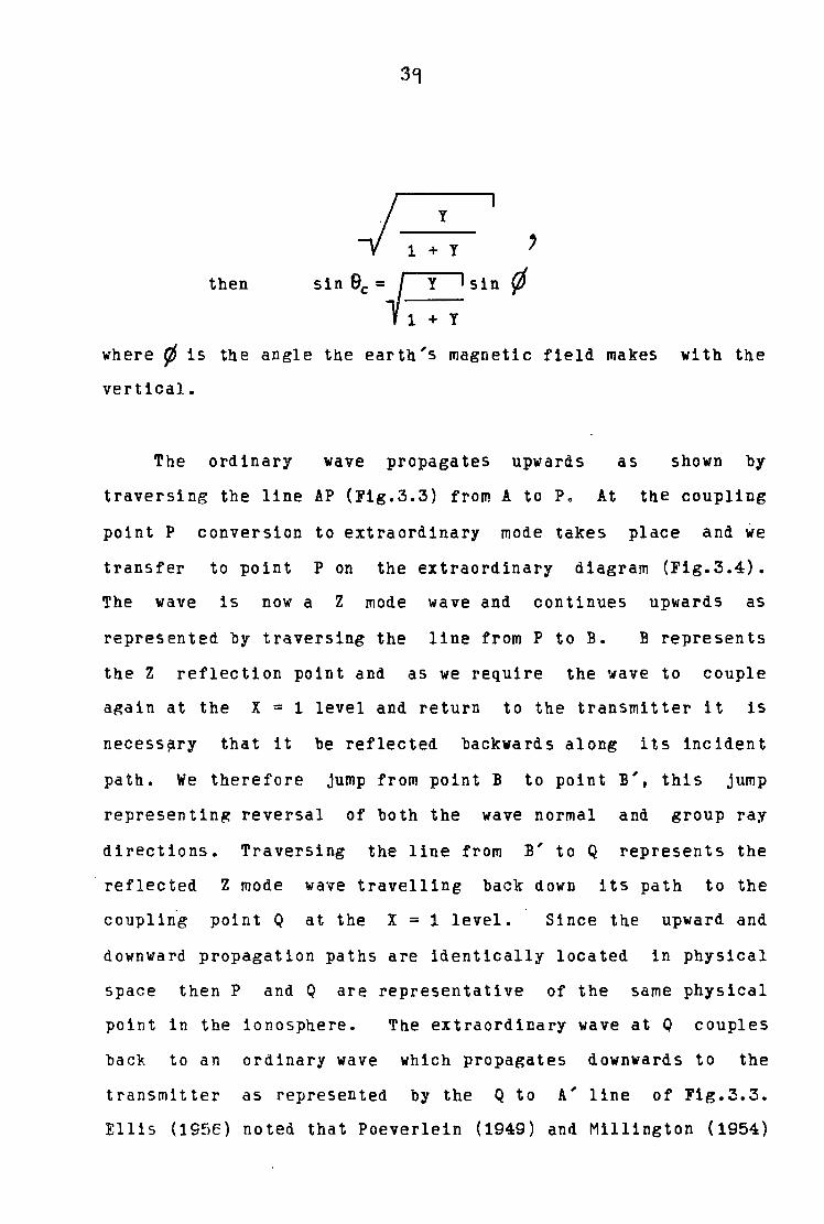
Ellis calculated the critical angle of incidence e, as a
function of frequency for different values of magnetic dip.
Fig.3.5 shows his results together with his observed directions
of arrival for Z echoes at Hobart. Fig.3.6 is a copy of one of
the records from Ellis's direction finder and it can be clearly
seen how closely the Z echo is confined to the magnetic
meridian plane.
So far collisions have been
non zero collision
propagation angle
frequency is
at which the
neglected. The effect
to increase from zero
transition from transverse
of a
the
to
longitudinal propagation occurs such that the X = 1 layer may
be penetrated by partial coupling of rays whose wave normals
make small angles with the magnetic field in the coupling
region. From an analysis of the distribution of Z echo angle
of arrival measurements, Ellis estimated the coupling cone to
be approximately circular and to have an angular half width of
a little under half a degree at 4.65 MHz wh~n the edges of the
cone are defined as the half power points. This further
confirmed the oblique incidence coupling theory of the Z mode
as the theory predicts that fixed relative to a single
radiating point on the ground there will be an effective "nole''
at the level X = 1 through which both the upward and downward Z
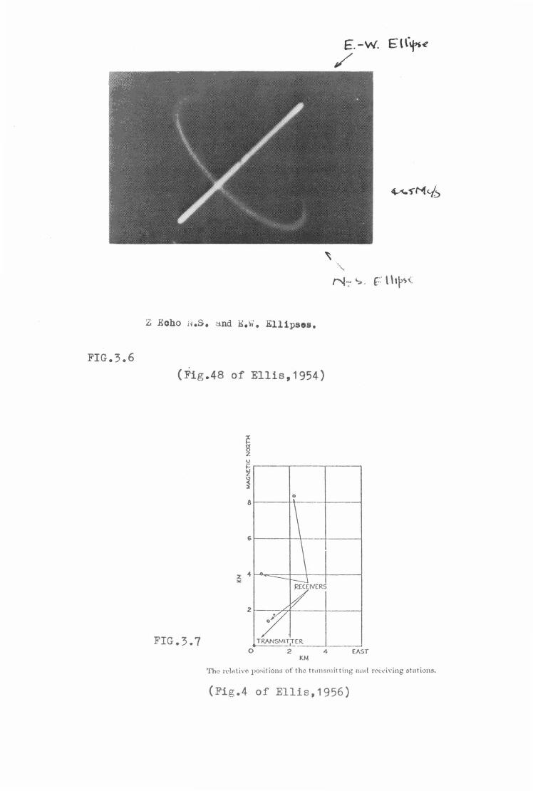
FIG.3.6
E. -w. E ( l"'f'~ /
., N-:- ~ . r · l \Ip~<.
Z Eoho H.S . 11nd }!;.~;. Ellipses.
(Fig.48 of Ellis,1954)
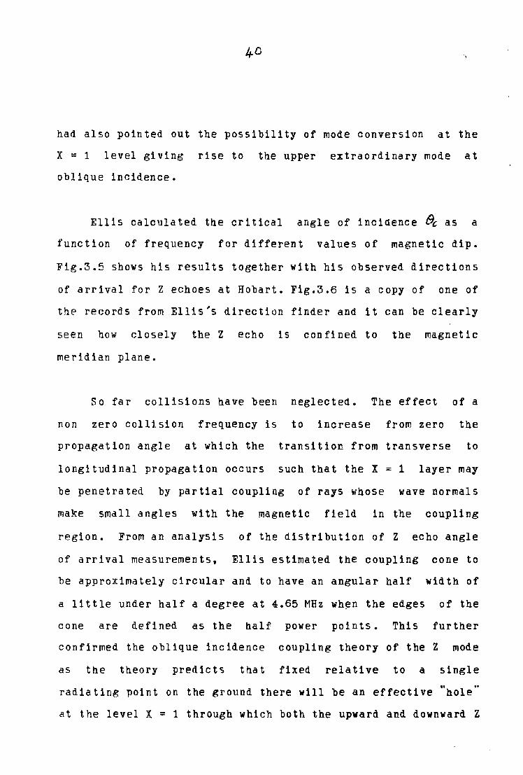
FIG.3.7
2
"'
~ 0 z v ~..--~~-,-~~-,-~~--, ., 7
~ 0
KM
Tho n•li\ti,•o po~itions of tho trnnsmit ting mul reel•i,·ing stations.
(Fig.4 of Ellis,1956)

rays must pass, downward rays not passing through this hole
being unable to reach the ground. Z echo amplitude will thus
fall quickly away from the transmitter and beyond a relatively·
short radius Z echoes will not be detectable. Ellis (1956)
provided experimental proof of this when he estimated the NS
angular ~idth of the Z hole by measuring the relative power of
simultaneous Z echoes at receivers spaced varying distances
from the transmitter. Fig.3.7 shows the location of the
receivers relative to the transmitter and Fig.3.8 shows the the
results achieved. The NS angular half width deduced from these
measurements is in good agreement with that deduced from the
angle of arrival measurements.
The oblique incidence coupling theory of the Z mode as
expounded by Ellis is widely accepted as tne correct
explanation of Z mode generation and the coupling region is
of ten referred to as the " " Ellis Window •
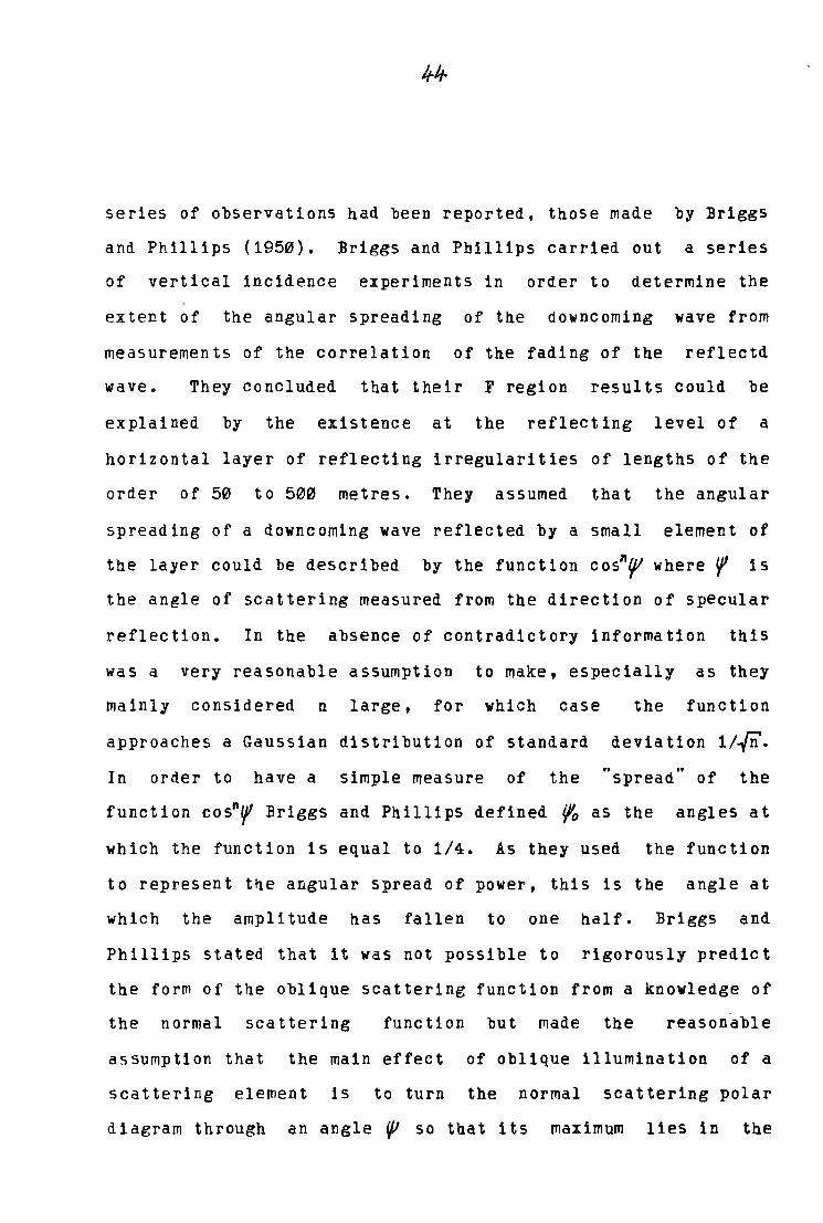
3o3 Return Of The Z Ray - Backscatter
Following a suggestion by Scott (1950), Ellis (1953b,1956)
proposed that the oblique incidence Z ray was returned to the
transmitter by backscatter from a rough ionospheric layer at
the reflection level. Fig.3.9 illustrates the return of the Z
ray. Ellis (1953b) examined · the a vai la ble · · evidence for
rou~hness in the ionospheric layer. At that time only one
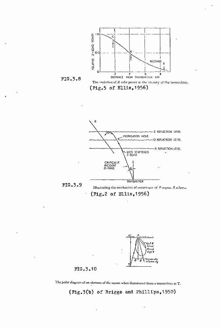
FIG.3.8
FIG.3.9
~- 10 LU
~ 0 :z: l!. I 05
N
I I o L.____ _ __ L_ _____ l __:-:_
2 4 b 8 DISTANCE FHOM iflANSM ITT EK Kt1
Tho ,-11riuti<1rt of Z crho powt'r m Ill<~ \"illllllf of tho trunsmittcr.
'(Fig.5 of Ellis,1956)
,......... f'ROPAGAT!m; HOLE ~-~--"'~--\- ~o REFLE<"TION LE'/El
CRITICALLT INCIDENT O·WAVE
TRANSMITTER
Illu:,trating the nwl'ha11i~m of occurrP11Ct' of f.'.rrg1on 7. cLhoc~.
(Fig.2 of Ellis,1956)
T
t'1.1rnc.:I
t~ ... j~ •n3r. e
FIG.3.10
The polar diagr<1m of an clement of the scrc~n when illuminated from a transmitter at T.
(Fig.3(b) of Briggs and Phillips,1950)
series of observations had been reported, those made by Briggs
and Phillips (1950). Briggs and Phillips carried out a series
of vertical incidence experiments in order to determine the
extent of the angular spreading of the downcoming wave from
measurements of the correlation of the fading of the reflectd
wave. They concluded that their F region results could be
explained by the existence at the reflecting level of a
horizontal layer of reflecting irregularities of lengths of the
order of 50 to 500 metres. They assumed that the angular
spreading of a downcoming wave reflected by a small element of
the layer could be described by the function cosnfjl where r is
the angle of scattering measured from the direction of specular
reflection. In the absence of contradictory information this
was a very reasonable assumption to make, especially as they
mainly considered n large, for which case the function
approaches a Gaussian distribution of standard deviation 1/...[Il.
In order to have a simple measure of the "spread" of the
function cosnr Briggs and Phillips defined ifo as the angles at
which the function is equal to 1/4. As they used the function
to represent t~e angular spread of power, this is the angle at
which the amplitude has fallen to one half. Briggs and
Phillips stated that it was not possible to rigorously predict
the form of the oblique scattering function from a knowledge of
the normal scattering function but made the reason'able
assumption that the main effect of oblique illumination of a
scattering element is to turn the normal scattering polar
diagram through an angle f/I so that its maximum lies in the
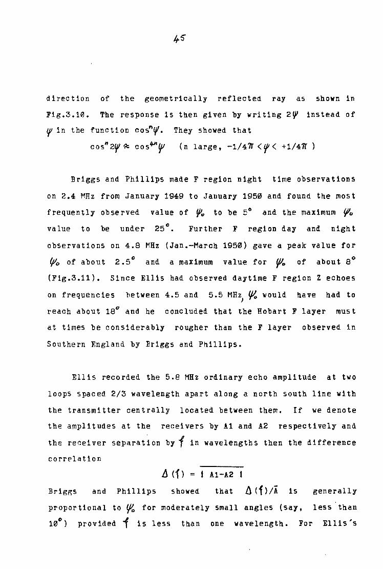
direction of the geometrically reflected ray as shown in
Fig.3.10. The response is then given by writing 2'/I instead of
'I' in the function cos"'f'. They showed that
cos11 2'f ~ co s"°"'f (n large, -1/47r <'f < +1/411' )
Briggs and Phillips made F region night time observations
on 2.4 MHz from January 1949 to January 1950 and found the most
frequently observed value of ¥'ci to be 5° and the maximum V'o value to be under 25°. Further F region day and night
observations on 4.8 MHz (Jan.-March 1950) gave a peak value for
(/lo of about 2 .5° and a maximum value for ¥'o of 0 about 8
(Fig.3.11). Since Ellis had observed daytime F region Z echoes
on frequencies between 4.5 and 5.5 MHz lJI,, would have had to )
reach about 18° and he concluded that the Hobart F layer must
at times be considerably rougher than the F layer observed in
Southern England by Eriggs and Phillips.
Ellis recorded the 5.8 MHz ordinary echo amplitude at two
loops spaced 2/3 wavelength apart along a north south line with
the transmitter centrally located between them. If we denote
the amplitudes at the receivers by Al and A2 respectively and
the receiver separatlon by f in wavelengths then the difference
correlation
/J Cf) = t A1-A2 I
Briggs and Phillips showed that /j ( f > ;i is generally
proportional to lfo for moderately small angles (say, less than
10°) provided -f is less than one wavelength. For Ellis 's
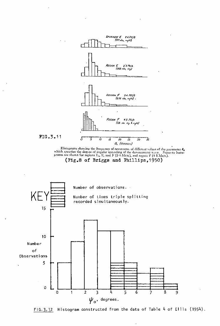
FIG.3.11
S.PoRA01c £ 2' Nels
a_rL..J.._....l.[~-L.L.l.-L_J__l==::J.(9-7'-o/,-•_· "J::'!=M=)===>- -
REGION £ Z 4 Meis
068 ""'· "'"!)
REGION F 2·4 Mc/s (233 oh1, ••7M) .
i, · __ R£c-1o_N_F __ 4_8_/o_1c-/s-----~~ (66 NI d7 & n'!At}
0 5 10 IS ZD 25 JO JS
()0 ( 0ECff.£'>)
Histograms shm,ing the fti:qu1·ncy of occurrencl of diffen·.1t \,1!ucs of the paiamctcr (J~ which spcc1tics the <lc1~1cc of angular spn·admg of the do\\ ncomin:: ".n c. S1•p:u 11<! h1sto· ~rams ar<! sho\1n for regions I·:,, E, :ind F (2·4 J\lc:s.), .md region F (·~ S :\lc/s.).
KEY~ 15 §
10
Number
of Observations
5
0 0
(Fig.8 of Briggs and Phillips,1950)
Number of observations. ·
Number of times triple splitting recorded simultaneously.
2 3 4
i/J degrees. To'
5 6 7 8 9
FIG.3. 12 Histogram constructed from the data of Table 4 of El 1 is (1954).

J;.1
experiment where f = 2/3 and Po was measured in degrees
Between the hours of 1300 and 1500 L.M.T. during the months of
July and August 1853, Ellis (1954) made measurements of A(f )/A
and thus obtained values for lfo. The results are shown in the
histogram of Fig.3.12 and superposed on it is a histogram of
the simultaneous occurrence of Z echoes on the h'f ionograms.
It can be seen that there is good qualitative agreement
between Z echo occurrence and increased values of the
'ionospheric roughness parameter lfo. Ellis concluded that
because of the very approximate nature of the roughness
measuring technique and because the theory did not take
possibly important secondary factors into account that an
attempt at a more detailed correlation of the occurrence of Z
echoes with ionospheric roughness was not warranted. Ellis had
observed an increase in Z echo amplitude near the critical
frequency and he suggested that en~anced scattering occurred at
this level and produced observable triple splitting at smaller
values of lfo than would otherwise be expected.
3.4 Critical Discussion
The term ,, ,, backscatter , when applied to contemporary
ionospheric sounding, usually means the return of radiowave
energy back along its incident path either by the process of
partial reflection or that of incoherent scatter. Partial
reflection occurs because the electrons have a distribution
that is irregular on a scale much greater than the distance
between them and much less than a radiowavelength; incoherent
or Thompson scatter occurs when energy is returned from
individual electrons, each scattering independently
(Ratcliffe,1972). Sounding techniques utilising these
backscatter processes require transmitters of very high power
and antennae of great sensitivity as the returned echoes are
very weak compared with the totally reflected waves detected by
traditional ionospheric sounding. Many workers, especially
before the advent of backscatter sounders, have employed the
term backscattering merely to denote that some radiowave energy
has been returned along an oblique incidence path by some small
irregularities near the reflection level. A particular
physical process has not always been specified and may not be
either of the partial reflection or incoherent scatter
processes but rather partial specular reflection in the
required direction. In this context I would suggest that the
term "small irregularities" means large enough to cause some
specular reflection at the irregularity yet small enough that
the ionosphere as a whole may still be considered as
essentially plane horizontally stratified. We may picture this
case as a flat ionosphere imbedded (at least in the vicinity of
the normal reflecting level of the sounding wave) with small
irregularities acting as tiny individual specular reflectors,
the direction of the reflected energy depending upon both the
direction of the incident energy and the orientation and shape
of the specular surface of the irregularity.
In the early and mid-1950's the available evidence all
pointed to backscattering from small irregularities at the
reflection level as being the most likely candidate for return
of the Z echo. Apart from the work of Briggs and
Phillips (1950), and the experiment of Ellis (1954) scattering
by small ionospheric irregularities was deemed resposible for
the results of many other experiments concerned with fading and
scintillations. Additionally Booker (1955), quoting previous
work, bad pointed out that not only might the scattered power
increase as the square of the mean ionization density (and the
greatest ionization density encountered is in the reflecting
stratum) but also that there existed the possibility of plasma
resonance of irregularities in or near the reflecting stratum.
He suggested scattering by irregularities in and near the
classical reflecting stratum to be nearly as important a
mechanism for returning energy as classical internal reflection
itself.
A greatly
reflection level
increased backscattering
would provide the required
effect at the
physical process
for the backscattering return mechanism of the Z ray. However
Pitteway (1958,1959) examined the scattered wave which
accompanies reflection from a stratified ionosphere in which
there are weak irregularities and considered the possibility of
enhanced scattering near the reflection level. He concluded
that any special resonance effect of tnis kind would be largely
destroyed by the collsional damping of the ionospheric
electrons. In 1958 Bowles carried out experiments at 41 MHz
verifying the existence of incoherent or semi-incoherent
scatter by free electrons in the ionosphere. As had been
expected, enormous sensitivity was required and Bowles used a
half megawatt (peak) transmitter feeding a 116 x 140 m antenna 0 of beam width 3.75 • His results showed a rise in noise level
peaking broadly at about 350 km. range but no noise peak
anywhere near the strength required to explain Z echoes in
terms of backscatter. Similar results are obtained by large
backscatter sounders which have since been constructed. The
requirement of great sensitivity in order to detect partial
reflection has also been confirmed by these sounders. It
becomes obvious then that in order to explain Z ray return by a
partial reflection or incoherent backscatter type mechanism a
reflection stratum resonance or similar enhancement phenomenon
must be invoked in order to amplify the Z echo to observed
levels. However in view of Pitteway's general findings it
appears highly likely that the suppression of such a phenomenon
under the Z mode conditions would be sufficient to prevent Z
echo signal levels reaching the strengths observed despite the
fact that the Z echo is usually observed as a relatively weak
signal.
51
We shall now examine the possibility of backscattering
from "small irregularities" of the type discussed in the first
paragraph. Of particular interest to this question are two
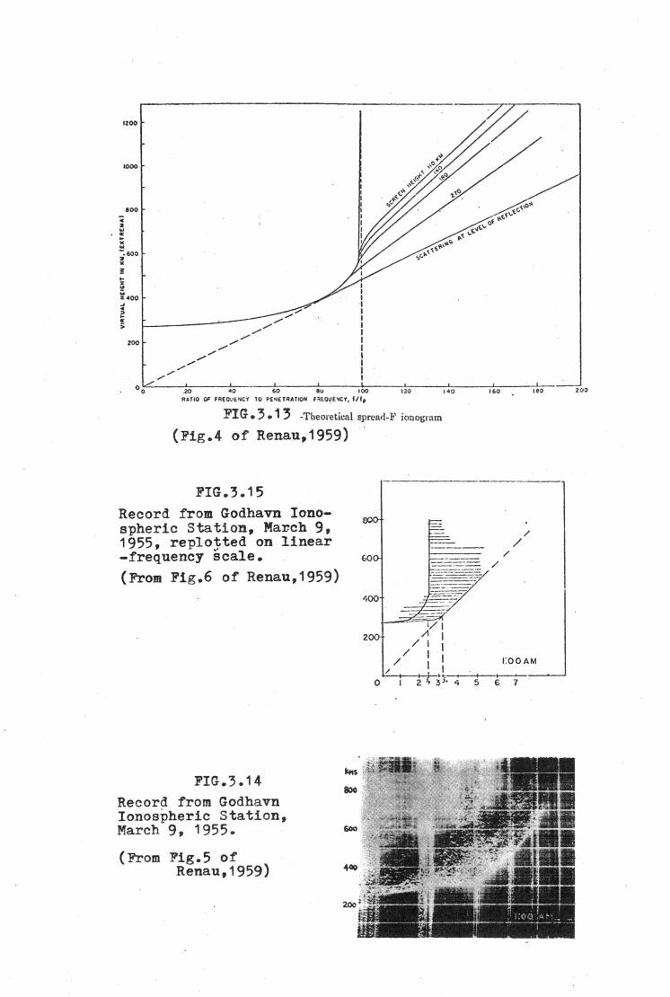
papers by Renau (1959,1960) in which he examined a theory of
spread-F based first on a scattering screen model and then on
aspect sensitive backscattered echoes. Renau (1959} based his
scattering screen model on a scattering mechanism of the type
discussed by Briggs and Phillips (1950}, referred to in the
previous section. This same scattering screen is thus of a
type which would be responsible for backscattered Z echoes.
The screen permits off vertical echoes to return to the sounder
and Renau made calculations of the virtual heights associated
with these oblique rays in order to establish the type of
ionogram that would result from such a model. He hoped that by
varying the height of the scattering screen he would obtain
some idea of the height principally responsible for spread-F
occurrences. Fig.3.13 shows the expected form of the ionograms
for various screen heights and included is the situation in
which
being
Ren au
the scattering
the situation
compared his
screen is at the level of reflection,
required for backscatter of Z echoes.
theoretical ionograms with actual
observations and found that the scattering screen theory could
satisfy a certain class of spread-F ionograms but not other
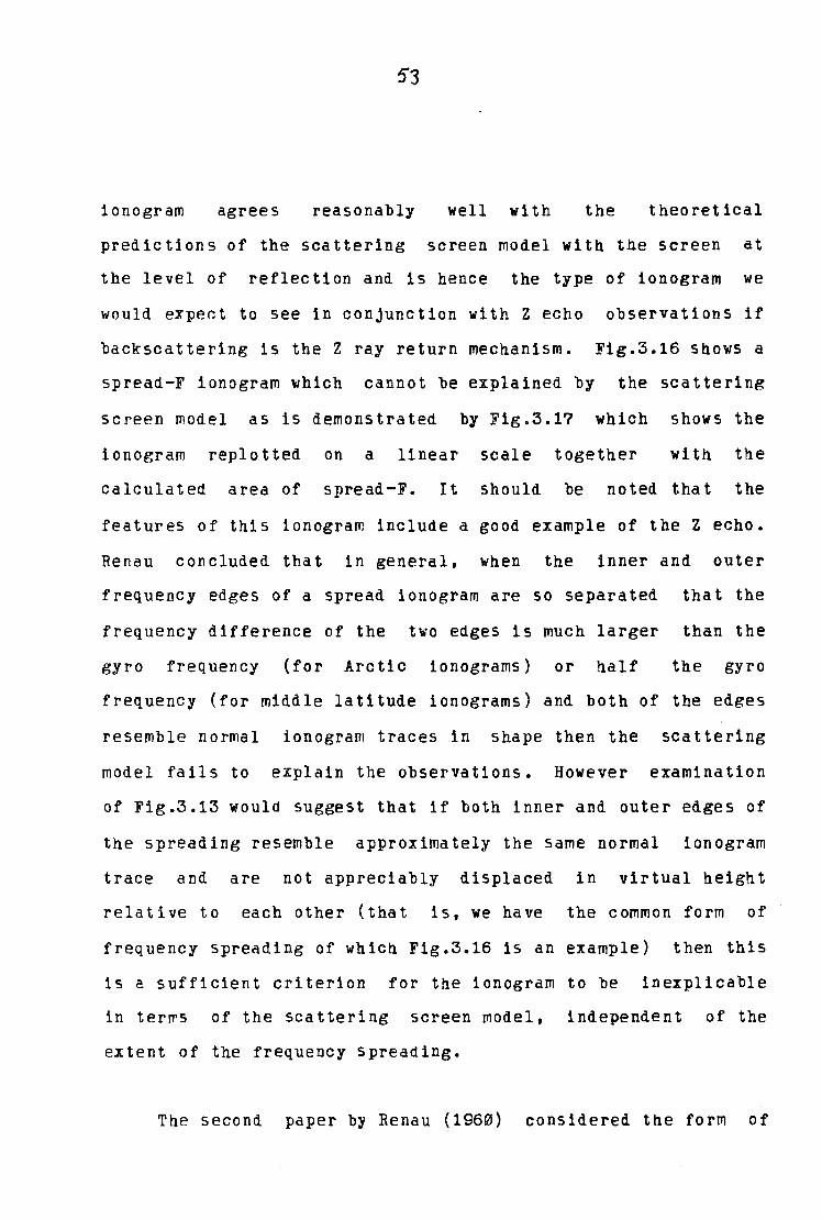
types. Fig.3.14 shows the spread-F phenomenon on a Godhavn
ionogram and Fig.3.15 shows it replotted on a linear scale
together ·with the
being indicated by
corresponding model, the observed spre~d
the horizontally shaded area. This spread
1200
1000
eoo c
" ... " ... " .. --IOO 2
" ! .. " .. ;;. :11:400 _, .. ;?
" > 200
"/
~------'-- ,,.,.,.,.,,.,,,,. /
,,,.,,,.
/ /
,,,.,,,.,,.,,,,.
a ~ ~ ~ 100
RATIO QI fAEOVE~CY 10 ° Pf.~£TAATtON fiflO~E~Y. flf, 120
FIG• 3 • 13 -Theoretical sprenrl-1" ionoi;ram
(Fig.4 of Renau,1959)
FIG.3.15
l•O 160
Record from Godhavn Ionospheric Station, Ma~ch 9, 1955, replojted on linear -frequency scale. (From Fig.6 of Renau,1959)
ljQO ,/
I/ I
/~ I 200
/ I I
/
/ /
uo
t:OOAM / I I 0 ,_/--+2-+,-31,-........ ,_.. ..... 5,__....,€r----7-----
FIG.3.14 Record from Godhavn Ionospheric Station, March 9, 1955.
(From Fig.5 of Renau,1959)
NO
53
ionogram agrees reasonably well with the theoretical
predictions of the scattering screen model with the screen at
the level of reflection and is hence the type of ionogram we
would exper.t to see in conjunction with Z echo observations if
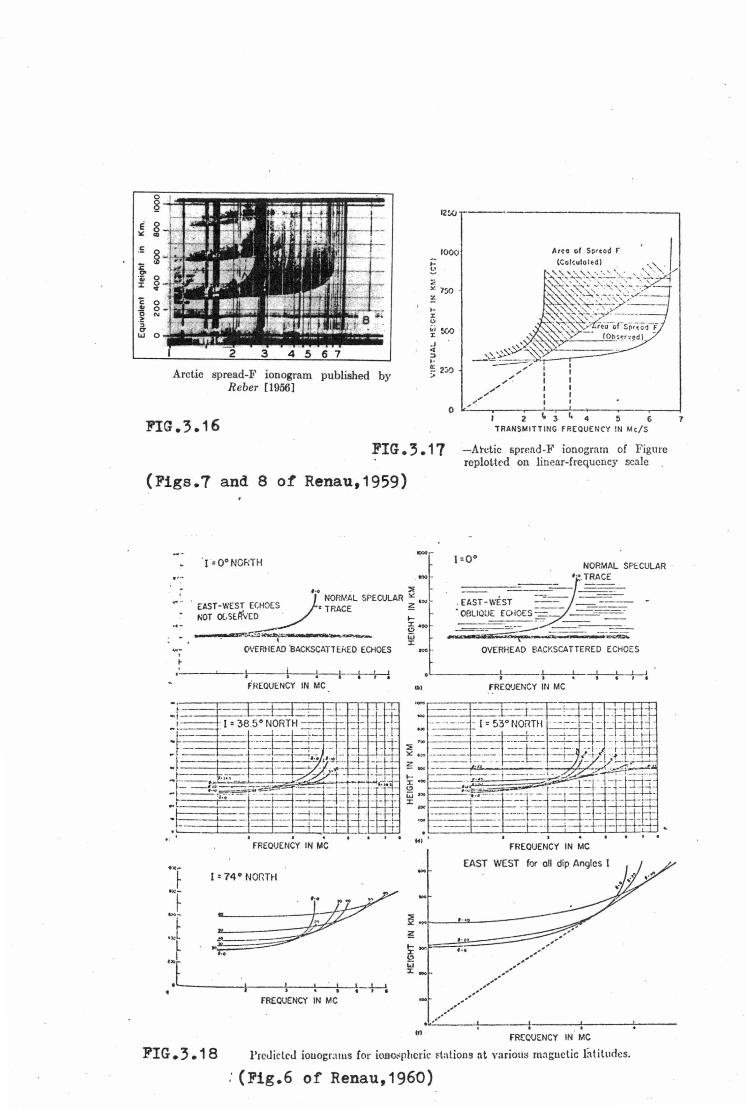
backscattering is the Z ray return mechanism. Fig.3.16 shows a
spread-F ionogram which cannot be explained by the scattering
screen model as is demonstrated by Fig.3.17 which shows the
ionogram replotted on a linear scale together with the
calculated area of spread-F. It should be noted that the
features of this ionogram include a good example of the Z echo.
Renau concluded that in general, when the inner and outer
frequency edges of a spread ionogram are so separated that the
frequency difference of the two edges is much larger than the
gyro frequency (for Arctic ionograms) or half the gyro
frequency (for middle latitude ionograms) and both of the edges
resemble normal ionogram traces in shape then the scattering
model fails to explain the observations. However examination
of Fig.3.13 would suggest that if both inner and outer edges of
the spreading resemble approximately the same normal ionogram
trace and are not appreciably displaced in virtual height
relative to each other (that is, we have the common form of
frequency spreading of which Fig.3.16 is an example) then this
is a sufficient criterion for the ionogram to be inexplicable
in ter~s of the scattering screen model, independent of the
extent of the frequency spreading.
The second paper by Renau (1960) considered the form of
0
~ 12!,() -------------------,
e 0 0
" CD
.!:
~
"' ·o; J:
c ... 0 > ·:; a UJ 0
... J:
1000
~ ~~ J
"' :> I ·
Arctic spread-F ionogram published by ~ 2~ Reber [1956]
0
Arco of Sprtod r
FIG.3.16 5 6
TRANSMITTING FREQUENCY IN Mc/S
FIG• 3 • 17 -Arctic sprcnd-F ionogrnm of Figure replotted on linear-frequency scale
(Figs.7 and 8 of Renau,1959)
.,_
.l ~~
] L
I =0°NORTH NORMAL SPECULAR · ... ... ~
-~ . ~NORMAL SPECULAR " , ..
EAST-WEST ECHOES TRACE ~ NOT OC..5ElfliEO 1-
6 400
~....:-~~..- w I J:
OVERHEAD BACKSCATTERED ECHOES
FREQUENCY IN MC
FREQUENCY IN MC
I= 74° NORTH
roo .
••• ~-----c}--------7,--7---~-!--~
fREQIJENCY Iii MC
• '----.....l.. __ ,__,_ _ _.. _ _.__.__.__.__._-7-"-7-'--'. 141 t
FREQUENCY IN MC
EAST WEST for oil dip Angles I
,,.I
.l ______ -l-----!--~--!---!~--f---1 FREQUENCY IN MC
FIG.3.18 l'rcJiclcJ iouoi;rams for iouo.~pl1cric Etalions :it various nrnguelic fatiludcs.
(Fig.6 of Renau,1960)
7
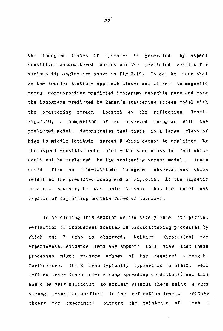
the ionogram traces if spread-F is
sensitive backscattered echoes and the
various dip angles are shown in Fig.3.18.
generated by aspect
predicted results for
It can be seen that
as the sounder stations approach closer and closer to magnetic
north, corresponding predicted ionograms resemble more and more
the ionograms predicted by Renau's scattering screen model with
the scattering screen located at the reflection level.
Fig.3.19, a comparison of an observed ionogram with the
predicted model, demonstrates tnat there is a large class of
high to middle latitude spread-F which cannot be explained by
the aspect sensitive echo model - the same class in fact which
could not be explained by the scattering screen model. Renau
could find no mid-latitude ionogram observations which
resembled the predicted ionograms of Fig.3.18. At the magnetic
equator, however, he was able to snow that the model was
capable of explaining certain forms of spread-F.
In concluding this section we can safely rule out partial
reflection or incoherent scatter as backscattering processes by
which the Z echo is observed. Neither theoretical nor
experi~ental evidence lend any support to a view that these
processes might produce echoes of the required strength.
Furthermore, the Z echo typically appears as a clean, well
defined trace (even under strong spreading conditions) and this
would be very difficult to explain without there being a very
strong resonance confined to the reflection level. Neither
theory nor experiment support the existence of such a
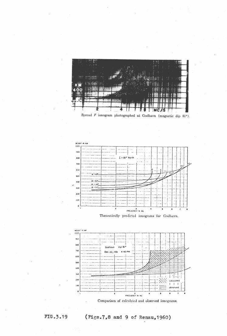
FIG.3 .19
Spread F ionogram photographed at Godhavn (magnetic dip 81°) .
• Ul Jl:(NCY 1-. MC •
Theorelically pre1Jictc1l ionograms for GoJha vn.
Comparison of calculult'J and obsen·cd ioncgrams.
(Figs.7,8 and 9 of Renau,1960)
57
resonance.
We are then left with the idea that Z echoes may be caused
by backscattering from the type of specularly reflecting
irregularities mentioned in the first paragraphs. This
conclusion is not entirely unexpected as Ellis (1954) used the
Briggs and Phillips (1950) two hundred metre estimate as an
indication of the expected average size of hi~ proposed F
region irregularities. Two hundred metres is several
wavelen~ths at the operating frequencies used by Ellis and thus
the irregularities are too large for the process of partial
reflection to operate satisfactorily. It can reasonably be
assumed that Renau's models also involve irregularities of this
type as he specifically references Briggs and Phillips when
introducing his scattering screen (Renau,1959).
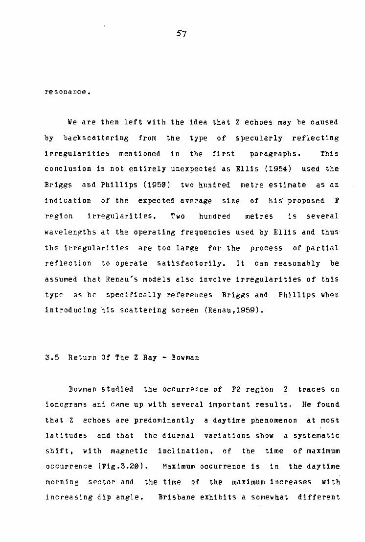
3.5 Return Of The Z Ray - Bowman
Bowman studied the occurrence of F2 region Z traces on
ionograms and came up with several important results. He found
that Z echoes are predominantly a daytime phenomenon at most
latitudes and that the diurnal variations show a systematic
shift, with magnetic inclination, of the time of maximum
occurrence (Fig.3.20). Maximum occurrence is in the daytime
morning sector and the time of the maximum increases with
increasing dip angle. Brisbane exhibits a somewhat different
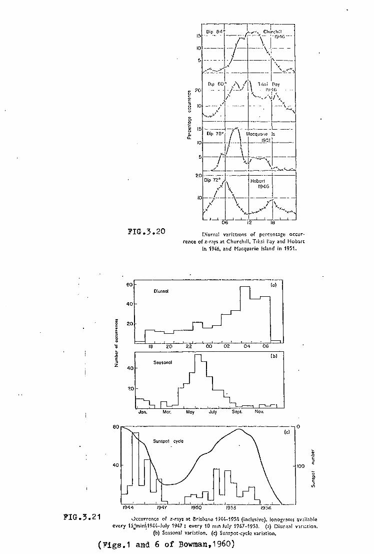
FIG.3.20
60 Diurnal
40
. .. 20 u c f .. " l: 0
0 .. u J)
E " z
40
Jon. Mar.
80
Sunspot
40
1944 1947
-r-Dip 04 ° , _ _,,,, Churchill
15 -- .... /.;}·----\- '"19'16 __ _
10 ----- --j-- ---\j --- --- -!) -- - - - ·,~/-- ---- -1'~-
..... Y .... ,.._,..,,.,. .... , '< .. -.-'1< ------- - -----.----- ,----.
Clip £10° 1\ !I\ l1~~i ,£la)' ?O I ~ I I' lf
10 ------,~-·/·-A -~·-~-~:~),~~\--/ ' X->(. ;x
~ -~~ . . g ---- ------+---___,
i 15 li;.-m·i T\ "~""':;;-,;--: _7~I1c-4=:;~--=
>..,, I ) .... "-""'"'-20 ______ _=-_.j ___ _i__ __ j_ ___ ,
Dip 7?/i\ 1 Hob1~~ 6 10 .!]-\~-- ----
-// x'x, '-"'"'x'j'" \,"-•,,.._, X-'<-'"'
_i__t-_ ---1 I . . 06 12 rs--'--'---'
Diurr.::! vari<:t1ons of percentage occurrence of z-rays at Churchill, Til:si l'0ay and Hoblrt
In 1946, and Macquarie Island in 1951.
22 ()() 02 04 06
May July
cycle
100
1950 19::>3 19~;n
~ ., n E ::> c
0 a. "' c ::>
VJ
FIG• 3 • 21 uccurrcncc of z-rays at ckisbanc 1·J44-19513 (inclusive). lonograms av.1il;ible every 15~min\1944-July 1947: every 10 min July 1947-1953. (a) Diurn:il vm~tion.
(b) Seasonal v:iriltion. (c) Sunspot-cycle vari.ltion.
(Figs.1 and 6 of Bowman,1960)
diurnal variation as Brisbane Z echoes occur mostly at night
although the maximum nevertheless occurs near dawn (Fig.3.21).
Seasonal variation revealed a winter maximum and a summer
minimu~ (Figs.3.22,3.21) and an inverse sunspot cycle
relationship was found to exist (Figs.3.23,3.21). A maximum Z
echo occurrence was found for magnetic dip angles of between
70° and 80° with a fairly quick fall off for lower and higher
dip angles (Fig.3.24). Eowman reported the presence of
spread-F in virtually every Z echo ionogram for Brisbane and 91
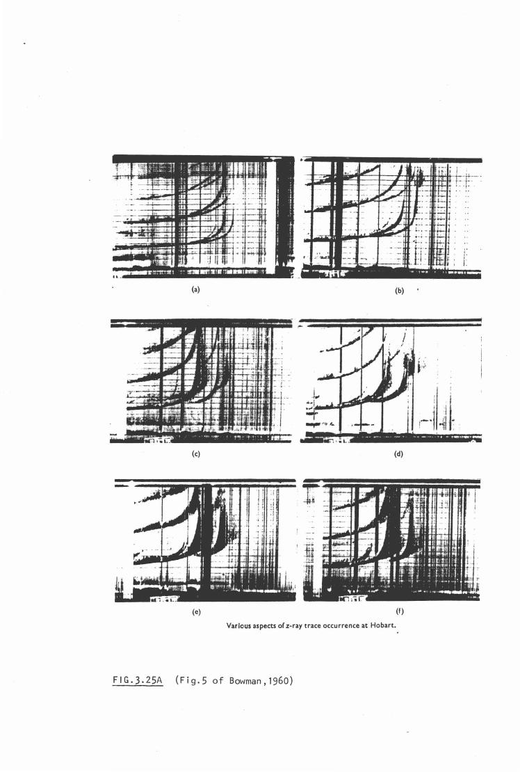
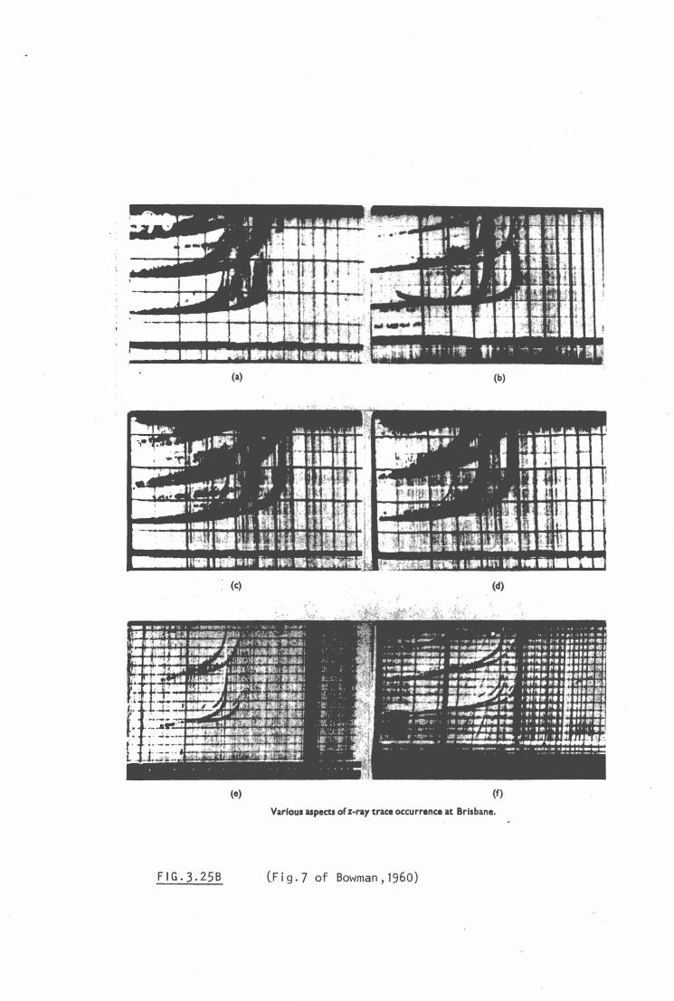
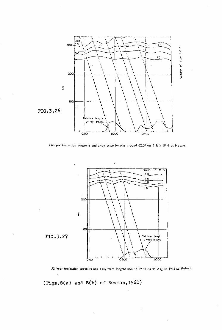
per cent of Hobart Z echo ionograms. He plotted contours of
equal ionization density for selected ionogram series by
calculating true heights and assuming all F2 layer reflections
to be vertical. On the same diagrams he also plotted the Z
ray trace lengths indicated by the ionograms and drew lines
along the positions of corresponding troughs or corresponding
crests and extended these lines to ground level as shown in
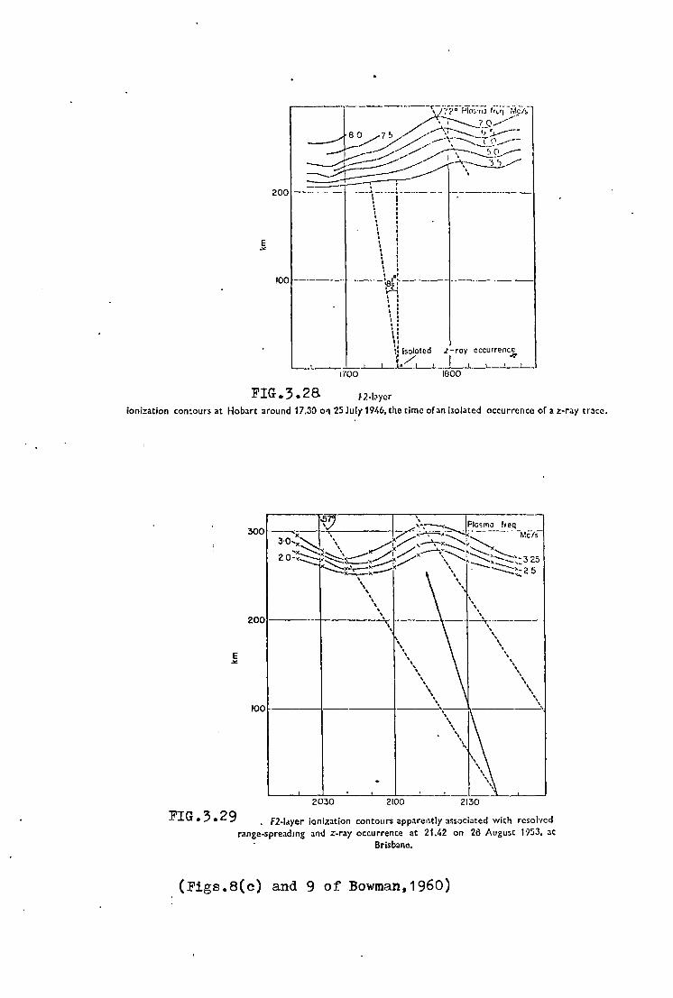
" Figs.3.2A and 3.2?. Bowman stated t~at an apparent
association between the upward slopes of ionization contours
and the occurrence of Z rays is revealed." Fig.3.28 is a thirn
diagram made by Bowman, this time for a single occurrence of a
Z echo at Hobart. Fig.3.29 shows ionization contours for a Z
echo occurrence at Brisbane.
Bowman found that the irregularities of his ionization
contours were the same sort of irregularities as those he
(Bowman,1960a) has suggested as being responsible for spread-F.
Fe noted that for Brisbane the diurnal,seasonal and sunspot
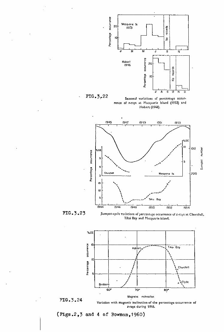
FIG.3.23
FIG.3.24
g ~
Macquarie Is a 20· 195'3 "' u 'O 0 ~
u .. ~ ,,, 0 10 0 c "' z ~ .. n. [-,-
_J..___j
J s N
"' u Hobarl r
1946 ~ ::>
"' u ~ " 0 0 u ..
10 ~ U> 0 0
~ z ~ ..
l-L Q.
J A s 0 N D
FIG.3,.22 Season:il variations of percentage occur-
.. u c
~
~ .. (.)' 0
c ., ~ .. Q.
re nee of z-rays at Macquarie Island (1953) and
Hobart (1946).
%GE
x'' 10 , , 100
"I.GE , , , I
' x 'x , , 9 ', ,.
', , , 5 ,x ', "
, .. 6 ',
' Ch"rctull
'x ... _ . 200 Macquarie Is 3 .__ ______ _
, 15 ',X ~I
' I \ , \ / \ ..c.----X'
\ ,'' ' " x,' T1k01 Bay ', /..-""' ----
10
5
.._~~~--i____J_~ L__
1944 l!HG 1948 1950 1952 1954
~ n E ::> c
0 l1.
"' c :>
V>
,Sunspot-cycle variations of percent«ze occurrence of z-r:i.1s at Churchill, Tiksi Bay and Macquarie Island.
"I.GE
t: 15 -----1----------t-·---,,~=~=,....--~---c Hobert , ........ -------........ x T1k~1 Boy
i }/' '\ 1011----~-----·---I -\-------i
I> I \ U> I \
~ I \ Churchill _, I \x
~ ,' \ ~ 51-----1--------.--, \
I ' / x \Cl)·dc
,,'' ', Brisbane '--l< I
60° 70° 80°
Mcgnehc 1nchnctiro
Vari.:tion with magnetic inclination of the percentage occurrence of z-rays during 1946.
(Fi~s.2,3 and 4 of Bowman,1960)
(a) (b)
(c) (d)
-
(e) (f)
Various aspects of z-ray trace occurrence at Hobart.
FIG.3.25A (Fig.5 of Bowman, 1960)
(a) (b)
(c) (d)
(e) (f)
Various aspects of z-ray trace occurrence at Brisbane.
FIG.3.25B (Fig.7 of Bowman,1960)
D.~= r · =-"":.-. ----;;;~=-~o --:I\ -:~~-o-~ ~\~-=r---~:- ---1 f~c~s \ i ' ' \ ----- ' ~----300 ~,... ~ \~-----.... --..::._- __.'.:..~
'\../" ---4__ ~ I _L_ \ \ · I -- --, 0 -, .....--;---l~I ' I --; :-' ~-------~ -7'"' \ ,, '
·' '~~ I~ ,__ ___ ,\ , ' I \ \ \_ ! ·-------~
\ \ \1 \ \ \{' . \ ' \ ' ' \ \ \ \ ' ', , ', \ I\ 200 ------ ---..... -------.. \--- --_\ ____ \: \, -----1~.\----·--· \ \ \ \ \ '. \ ·\ ', \ \ \ \ \ \ \ \ \ \ \ \ \\1 \ ' ' \ ' ' ' ' ' ' ' ' l \ \ \ \ \ \ \
100---·1·----\------\1-----.:\-, --\--\:1---\-. \ \ \ \' \
' ' \ ' ' ' ' ' ' ' ' \ ' I ' ' ' ' ' \ I \ \' \ \ \ \
Relative length \ I \ \ \ \ _ \ I r-roy troc~{><-~,~, \ \ \ /x x~, I ,.. } \ /~~--~. '\~_,
.__._ _____ __... __ _,,__,~_,·.._._ ,~! v~-~ , J
E .x:
FIG.3.26
0100 0200 0300
" •. ., r
~ " u u 0
'.. -'"' E :> ....
F2-la.ycr ionization contours and z-ray trace lengths around 02.CO on 4 July 1946 at Hobart.
E -X
FIG.3.27
-...L~-----~----Plo;:no - f rea M:/s
\ \ \ \ · 30 1
_.,__+..___" ~ ----2 5 ! ~ -;---_,.,.....---........_~ -----------~
\ \ \ ~ \ \ \ \ 15 \ ' ' ' \ \ \ ',
\ \ ' ' \ \ '\ \ 200 ~-j-----''r\ --.,- -L,--T----'"--\ -----
\ ' ' \·
100
0100
\ \ \ ' \ \ \ \ ' ' ' ' \ '. \ \
\ ' ' ' \ \ ' ' ' ' ' \ \ ' \
\ \ \ \ \ \ ' \
~---'L,-----\,-,-~~--~~-+--~I • . I • , ' ' ' ' ' ' \ ' \ 1 , ' Relol1ve lenglli
\, j\ \ \ z/-rO)' troces
' ' ' ' \I " I •
0300
Fl-layer ioni=ation cortours and z-ray trace lengths around 02.00 on 11 August 19-:6 :it Hobart.
(Figs.8(a) and 8(b) of Bowman,1960)
200
E ""'
100
----'('"--·-------- ------ - -, /?(' 0 Pl11:.·11•J f1«1 l~l_s:I>
/.:?"---__7__Q _......-' 7'> /~.......--'·~ 1,~
..r ' -:,,,,/ / ,..--·\--........ --, p --_/ .// _.,,/ \ --- ..------ / _..../ ~~~~-.....-
--:::.......--~ -\---:D-/ ~-- \ --------C- I
' I ----. -- - ---..J,-----i------- ---· --------- -
i I I . I I I I I I . \ I I . . •' ------ ----\a~:----,_...,
I I I I
I ' ~ : I: I I .. .. •• ,, \: Isololcd .z-roy occurrence •'/ I ~ _j_~~-L_L._,.;__,___... __ _..__..__,
1700 1800
FIG. 3. 2 8. f2·l~ycr ionization contours at Hobart around 17.3:> 0'1 25July1946, the time of an isolated occurrence of a z-ray trace.
E ""
FIG.3.29
2001-----+------>.,-i-
2030 2100 2130
. F2-1.i.yer ionization contours apparently associated with rcsol·(cd range-spreading and z-ray occurrence at 21.42 on 28 Augu5t 1953, at
Brisbane.
(Figs.8(c) and 9 of Bowman,1960)
cycle variations for Z echoes were very similar to those for
spread-F; for Hobart the seasonal variations were the same; and
for Macquarie Island the winter maximum and summer minimum of Z
echoes was the same as that found at high latitudes for
spread-F. Since very high latitude spread-F had been reported
to vary directly with sunspot activity, Bowman concluded that
the sunspot cycle variations for spread-F and Z echoes would be
dissimilar at stations such as Churchill and Tiksi Bay.
Bowman (1960a) had previously suggested that kinking of
the ionization contours of the F2 layer were responsible for
spread-Fat middle latitudes and as he had found such a strong
association between spread-F and Z echoes he made the further
suggestion that the return of the Z ray might result from the
same kinking. He postulated that the spread-F irregularities
could have extended fronts aligned perpendicularly to the
magnetic meridian such that t~e Z wave could possibly be
reflected back along its path, in the plane of the magnetic
~eridian, because of the sloping ionization contours of the
irregularity. The ionization contours may remain approximately
horizontal up to the normal 0 ray reflection level as the only
requirement is that the ionization contours above this level
should be so shaped that a ray which is longitudinal at the 0
reflection level and passes through the coupling cone will be
normal to tne ionization contours when it reaches the Z mode
reflection level.
Using the Poeverlein diagrams Figs.3 & 4 of Ellis (1953b)
Bowman traced ray paths in the two types of model ionization
distributions, one corresponding to a Figs.3.26 and 3.27 type
distribution ("spread-F irregularity") and the other
corresponding to Fig.3.28 ("sunset period"), and found
ionization distributions which satisfied the requirements that
the ray path allowed longitudinal propagation at the X = 1
level and normal incidence to the layers
level. The angle of incidence for the
was 8.5° and that for the "spread-F
(Figs.3.30,3.31).
3.6 Critical Discussion
at the Z reflection
" " sunset period model
irregularity", 0
14
Bowman's (1960) paper makes firstly sorne useful
contributions to knowledge of the morphology of the Z echo and
secondly proposes an alternative mechanism for the return of
the Z ray. On a cautionary note it should be remembered that
~uch of Bowman's information on the morphology of the Z mode
has been gathered from other papers and publications and there
has been no standardisation or cross comparison of the scaling
or ionosondes of the stations involved. The Z mode can be a
very difficult parameter to scale and high latitude ionograms
can be very hard to interpret. Variations in sounding
equipment may affect the relative occurrence on the ionograms
of weak phenomena such as the Z mode. In the past the Z mode
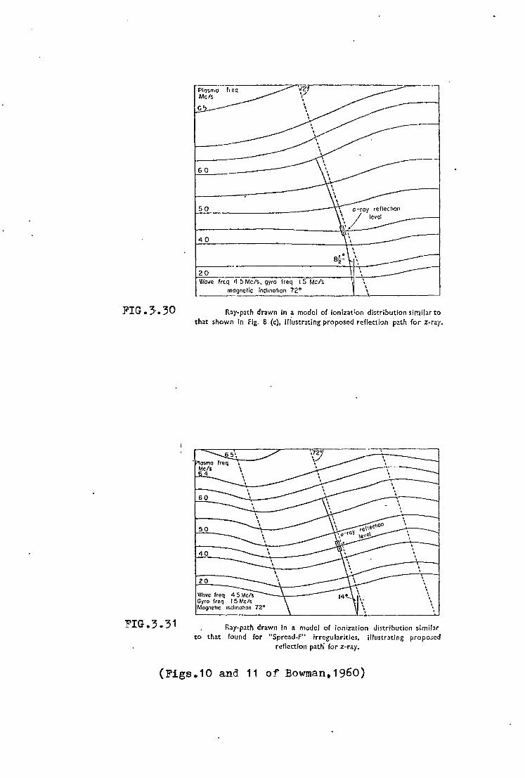
FIG.3·.30
FIG.3.31
Plosnio Meis
G'>
60
50
40
20
Ir cq ~·112· t/ I
' I ' ' ' '
Woo1e frtq <1 ~Meis, gyro freq I 5 Meis magnetic inclinot1on 72° ----
Ray-path drawn in a model of ionization distribution similar to that shown in Fig. 8 (c), ilfustrating proposed reflection p<!th for z-ray •
50
40
20
Wove freq
. ' I
\
\
' ' '
Gyro freq I 5 W.c/s Mag.iehc mcl1notton 72°
. . . . ', ' '. . ' . .
' \ \ . . .
Ray-path drawn in a model of ionization distribution sirnibr to that found for "Sprcad-F" irrcgubritics, illustrating propo;cd
reflection patli for z-r;;.)".
(Figs.10 and 11 of Bowrnan,1960)
68
has not always been correctly identified. Rivault (1950), for
instance, reports seeing the Z mode mainly on the second order
reflections but on examination of the ionograms illustrating
his paper it appears the Z mode is being confused with
satellite traces and is not in fact present.
Bowman's Z ray return mechanism is a sound alternative to
the backscatter mechanism. Probably its most important feature
is that return of the Z ray along its path at the upper X mode
reflection level takes place by the usual total reflection
process thereby avoiding t~e confusion over whether or not
backscattering will provide an echo of the observed strength.
Bowman takes note of Ellis's experimental evidence, suggesting
that most of the tilting would occur above the 0 ray reflection
level and noting that one of the two calculated angles of
arrival is larger than those observed by Ellis. Bowman links Z
mode occurence with that of spread-F and suggests that his
ionization contours would be responsible for both phenomena.
Strong backscattering, however, would also be expected to
produce spread-F. Tne tilt mechanism is a very worthwhile inea
as there seems to be no doubt that the Z ray would be returned
if the appropriate ionospheric configuration occurred.
The rnain problem with the tilt theory is that it is an
extremely restrictive model in that it must not only return the
oblique Z ray back along its path but it must also provide for
upgo1ng and downgoing Z rays to have their wave normals making
0 no more than 1/2 angle with the magnetic field at the O mode
reflection level. An important consequence of these conditions
is that the Z ray is for all practical purposes confined to the
magnetic meridian at least up to the coupling point. Bowman's
paper does not address. the question of whether or not the
special combination of tilts required might occur sufficiently
often to account for the observed frequency of Z mode. Tilts
unquestionably occur in the ionosphere (e.g. Munro,1953) and
relatively frequently but tilt observations indicate that the
larg~r tilts (such as the 18+ 0 required at the Z reflection
level) occur only rarely and the requirement that such tilts be
in the magnetic meridian may mean that the required conditions
occur much less frequently than the Z echo except at very high
latitudes where the tilt requirements are smaller and the Z
echo occurs less frequently according to Bowman (Fig.3.24). As
insufficient is known about the statistical occurrence af the
various ionization contour perturbations the answer to this
problem must be an experimental one. Bowman (1960) claimed to
have observations supporting his alternative. However there
are so~e serious objections to the method of analysis and these
are detailed as follows :
A) A multi-point (Schmerling 5 pt. and 10 pt. method)
method of estimating true heights has been used. These
methods are valuable for estimating the true height of a
particular event but great care must be exercised when
making true height versus time plots as these methods do not
usually provide the required accuracy. For example, subtle
changes in the underlying layers, especially if accompanied
by partial cusp development, may produce apparent variations
in the true heights of higher levels which do not
necessarily bear any resemblance to the real variations.
Reliable real height versus time plots of the type attempted
by Bowman require high repetition frequency of ionograms
(e.g. one per minute), first class ionograms showing very
little perturbation and appropriate high accuracy real
height reduction techniques. Unfortunately under quite
perturbed conditions such as those postulated for the
occurrence of Z mode the required accuracy is normally
unattainable. Errors in the multi-point height method will
tend to correspondingly raise or depress values at other
levels so that the shape correspondence of various
ionization contours is no valid check on the accuracy of the
result.
If Figs.3.26 to 3.28 are taken from i~nograms at 10
minute intervals (as would appear to be the case though I
was unable to obtain the original records) then we have only
four readings per ·quasi-periodic cycle of the ionization
contours and it is doubtful that peaks and trpughs could be I
seen to be aligned at a certain angle, given so little
information. If appropriate error bars were put on the
height points it might be hard to justify the positioning of
the peaks and troughs. In any case examination of the
contours as drawn reveal
fit very well
direction.
along
71
that the peaks and troughs
the dashed magnetic field
do not
line
These, however, are relatively minor quibbles compared
with the following objections.
B) Assuming that the real height analysis is correct,
no justification has been given for the unstated assumption
that what is being viewed is travelling wave motion in the
ionosphere and not simply bulk vertical motion of the whole
or part of the F2 region.
C) Assuming that the real height analysis is correct
and assuming that the results represent travelling
horizontal and not bulk vertical motions in the ionosphere
then no justification has been given for the again unstated
assumption that the travelling motion is not only along the
magnetic meridian but furthermore is in the correct
direction along that meridian. In addition, for successful
Z mode propagation there may be no east-west (magnetic)
tilts across the magnetic meridian below the X = 1 level in
order that the Z ray wave normal be parallel with the
magnetic field at this level. It could be argued that a
particular lateral vertical distribution of ionization could
allow significant east-west tilts yet still fulfill this
condition but in view of the already restrictive nature of

72
the tilt model in the magnetic meridian it would be such an
extremely unlikely possibility that it can be ignored. In
short, the tilt model will probably have difficulty
satisfying reasonable electron density distributions without
introducing unreasonable ones. Large east-west tilts above
the X = 1 level are more likely but nevertheless impose
further restrictions in that they must allow the Z ray to
retrace its path to the coupling region.
D) Assuming all the preceding objections to be
satisfied there will be O mode and X mode reflections from
a~proximately the same region of the ionosphere as that
producing t~e Z mode. Bowman has stated the assumption that
all F2 layer reflections are vertical and this is clearly
not a good assumption under the circumstances (there may or
may not be additional reflections from overhead deperiding
upon whether or not the overhead contours are horizontal).
For instance the 3 MHz 0 mode echo at 0155 hrs ,4/7/46HO
(Fig.3.26) would be coming from around the 0105 hrs region
and thus the "true heights" of such times/points are well
out. In other words, the results are found to invalidate
this assumption.
Assume all the preceding objections to be satisfied -
the following further objections apply :
E) The Z mode length graphs as drawn in Figs.3.26 and
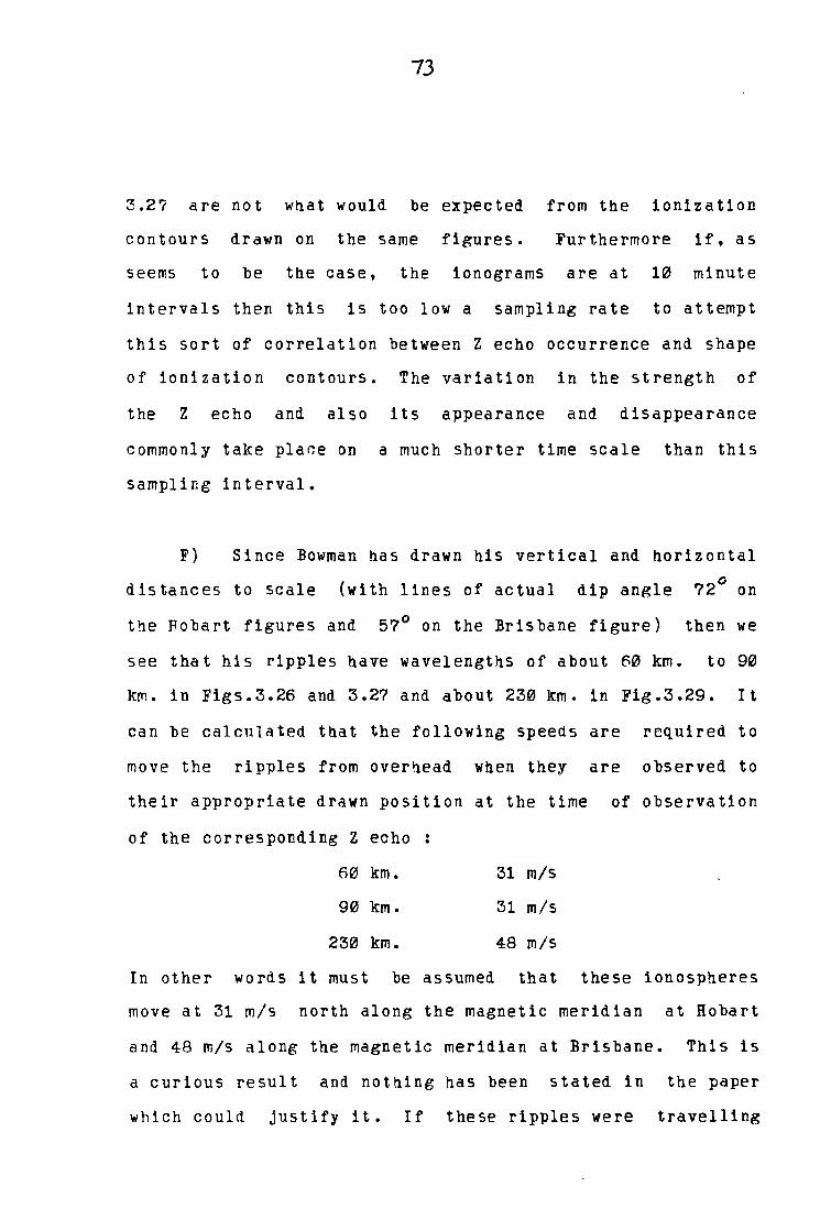
3.2? are not what would be expected from the ionization
contours drawn on the same figures. Furthermore if, as
seems to be the case, the ionograms are at 10 minute
intervals then this is too low a sampling rate to attempt
this sort of correlation between Z echo occurrence and shape
of ionization contours. The variation in the strength of
the Z echo and also its appearance and disappearance
commonly take place on a much shorter time scale than this
sampling interval.
F) Since Bowman has drawn his vertical and horizontal
distances to scale (with lines of actual dip angle 72° on
the Fobart figures and 57° on the Brisbane figure) then we
see that his ripples have wavelengths of about 60 km. to 90
km. in Figs.3.26 and 3.27 and about 230 km. in Fig.3.29. It
can be calculated that the following speeds are required to
move the ripples from overnead when they are observed to
their appropriate drawn position at the time of observation
of the corresponding Z echo
60 km.
90 km.
230 km.
31 m/s
31 m/s
48 m/s
In other words it must be assumed that these ionospheres
move at 31 m/s north along the magnetic meridian at Hobart
and 48 m/s along the magnetic meridian at Brisbane. This is
a curious result and nothing has been stated in the paper
which could justify it. If these ripples were travelling
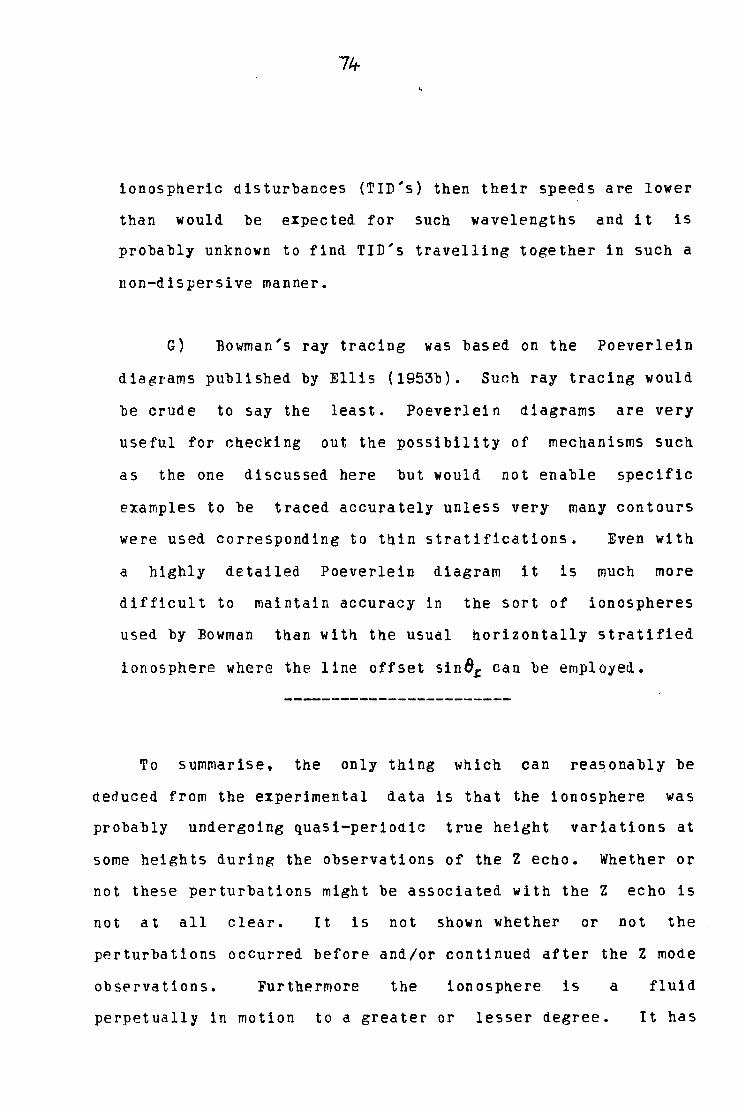
ionospheric disturbances (TID's) then their speeds are lower
than would be expected for such wavelengths and it is
probably unknown to find TID's travelling together in such a
non-dispersive manner.
G) Bowman's ray tracing was based on the Poeverlein
diagrams published by Ellis (1953b). Such ray tracing would
be crude to say the
useful for checking
least. Poeverlein diagrams are very
out the possibility of mechanisms such
as the one discussed here but would not enable specific
examples to be traced accurately unless very many contours
were used corresponding to thin stratifications. Even with
a highly detailed Poeverlein diagram it is much more
difficult to maintain accuracy in the sort of ionospheres
used by Bowman than with the usual horizontally stratified
ionosphere where the line offset sin8L can be employed.
To summarise, the only thing which can reasonably be
deduced from the experimental data is that the ionosphere was
probably undergoing quasi-periodic true height variations at
some heights during the observations of the Z echo. Whether or
not these perturbations might be associated with the Z echo is
not at all clear. It is not shown whether or not the
perturbations occurred before and/or continued after the Z mode
observations. Furthermore the ionosphere is a fluid
perpetually in motion to a greater or lesser degree. It has
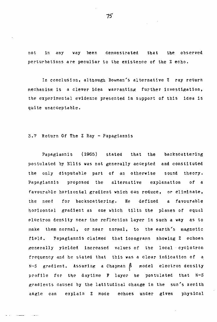
75'
not in any way been demonstrated that the observed
perturbations are peculiar to the existence of the Z echo.
In conclusion, although Bowman's alternative Z ray return
mechanism is a clever idea warranting further investigation,
the experimental eviden~e presented in support of this idea is
quite unacceptable.
3.? Return Of The Z Ray - Papagiannis
Papagiann is (1965) stated that the backscattering
postulated by Ellis was not generally accepted and constituted
the only disputable part of an otherwise sound theory.
Papagiannis proposed the alternative explanation of a
favourable horizontal gradient which can reduce, or eliminate,
the need for backscattering. He defined a favourable
horizontal gradient as one which tilts the planes of equal
electron density near the reflection layer in such a way as to
make them normal, or near normal, to the ~arth's magnetic
field. Papagiannis claimed that ionograrns showing Z echoes
Renerally yielded increased values of the local , cyclotron
frequency and he stated that this was a clear indication of a
N-S gradient. Assurring a Chapman ~ model electron density
profile for the daytime F layer he postulated that N-S
gradients caused by the latitudinal change in the sun's zenith
angle can explain Z mode echoes under given physical
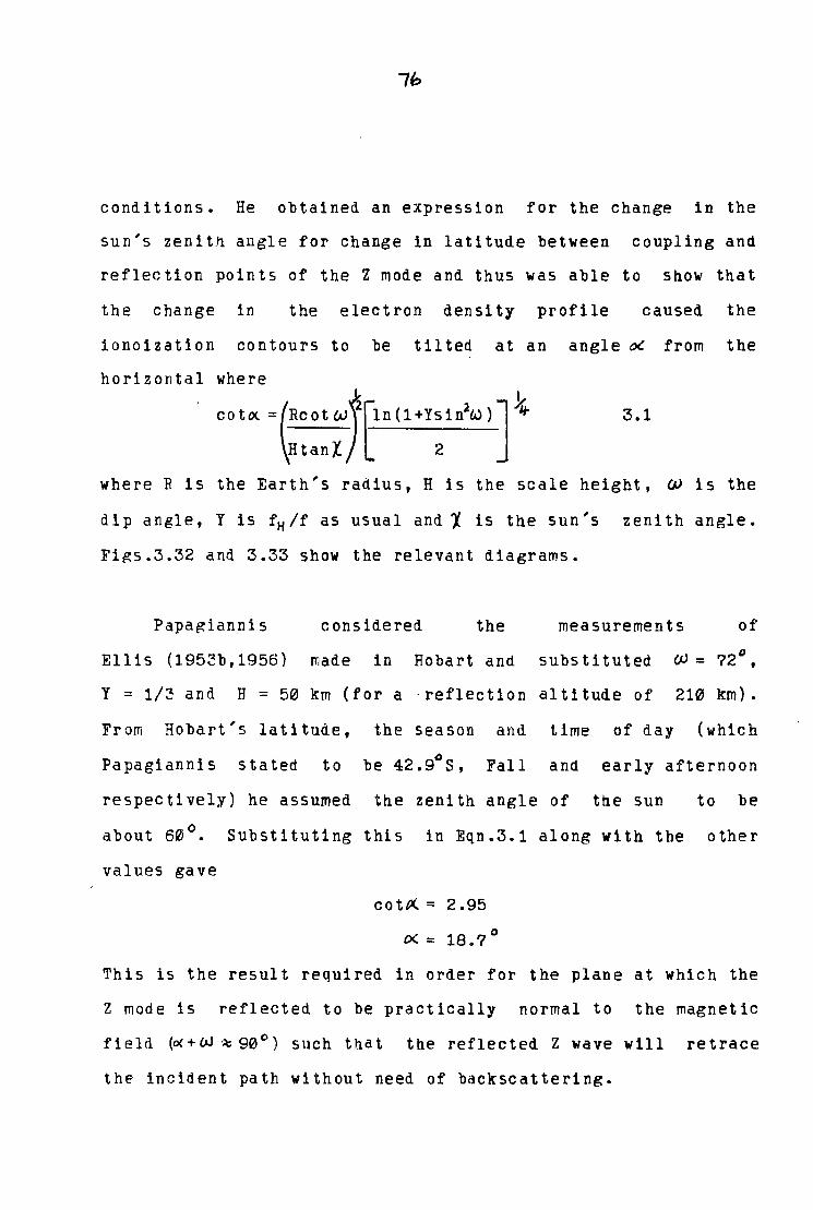
7h
conditions. He obtained an expression for the change in the
sun's zenith angle for change in latitude between coupling and
reflection points of the Z mode and thus was able to show that
the change in the electron density profile caused the
ionoization contours to be tilted at an angle oe from the
horizontal where
co toe. =(Re ot wJ[1n ( 1 +Ys in2w) J ~
HtanX L 2
3.1
where R is the Earth's radius, His the scale height, w is the
dip angle, Y is fH /f as usual and"/.. is the sun's zenith angle.
Fi~s.3.32 and 3.33 show the relevant diagrams.
Papa~ian.ni s considered the measurements of
Ellis (195~b,1956) made in Hobart and substituted (JJ = 72°,
Y = 1/~ and B = 50 km (for a -reflection altitude of 210 km).
From Hobart's latitude, the season and time of day (which
Papagiannis stated to 0 be 42. 9 S, Fall and early afternoon
respectively) he assumed the zenith angle of the sun to be
about 60°. Substituting this in Eqn.3.1 along with the other
values gave
cottX. = 2.95
{)(. = 18 0 7 ° This is the result required in order for the plane at which the
Z mode is reflected to be practically normal to the magnetic
fielcl (o<+W ~ 90°) such th.at the reflected Z wave will retrace
the incident path without need of backscattering.
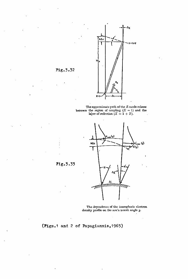
Fig.3.32
Fig.3.33
Htu --..( __
X=I
The approximate path of the Z-mode echoes between the region of coupliug (X = 1) and the
Ia;rcr of refirction (X = l + Y).
Hlu -......... ......... >---11.1 N'ma• <x'> N'lxl
Tho dopcnrlcnco of tho ionospheric electron density profile on the sun's zcnit..h nnglo X·
(Figs.1 and 2 of Papagiannis,1965)
7'6
Papagiannis allowed that the near perfect numerical
agreement obtained is undoubtedly beyond the general accuracy
of the computation presented but considered that the result
nonetheless is a convincing argument in favour of the proposed
theory. He stated that Equation 3.1 shows that at a given
location the angle ot. is a function of the angle l (i.e. a
function of the sun's zenith angle) and that this is in
agreement with Ellis's measurements which suggest that Z mode
echoes are observed during consecutive days at nearly the same
local time. He noted that Eqn.3.1 also shows that as we
advance towards the equator ttie angle IX aecreases whereas
(90-w) i~creases, making the a~pearance of Z mode echoes
progressively more difficult, which is also borne out by
observations.
Papagiannis obtained a simple relation between IX and W by
assuming that the sun's zenith angle X is approximately equal
to the geomagnetic latitude so that for a dipole magnetic field
the Eqn.3.1 reduces to
tanW ~ 10tano<. 3.2
Sine~ Eqn.3.2 clearly shows the previously mentioned latitude
effect he concluded that Eqn.3.1 is in basic agreement with the
available observational results. Papagiannis stated that
although one could try to derive a more precise expression for
the angleoc.., the horizontal gradients of electron density are
not always caused by the sun's varying zenith angle and thus
this refinement would not be very meaningful. He considered
that it would be more profitable .to try to verify the process
by ray tracing the Z mode using several electron density
profiles with chosen horizontal gradients at various magnetic
latitudes to yield the range and type of graaients required by
his proposed theory.
Papagiannis suggested that
experimentally by a system of
along the magnetic meridian and
his theory could be tested
ionospheric sounders located
measuring the N-S horizontal
gradient of electron density whenever Z echoes are observed.
He noted that the deflection of tne ordinary rays towards the
pole and of the extraordinary rays towards the equator can be
used very profitably in interlacing the system of ionospheric
sounders.
3.8 Critical Discussion
The idea proposed by Papagiannis explains the Z mode in
terms of solar radiation generated tilts in t~e ionosphere and
the resulting ionospheric model thus becomes a special case of
the Z ray return mechanism suggested ~y Bowman (1960).
Certainly, if the ionosphere at Hobart behaves as Papagiannis
has numerically predicted then it will be an ideal ionosphere
for return of the Z mode, the magnetic field being
perpendicular to the stratifications. But t~ere are some
objections and qualifications to Papagiannis's proposal,
80
detailed as follows
A) Perhaps somewhat surprisingly in view of all· t~e
qualifications to the assumptions of the Chapman Layer
Theory, the E and Fl layers behave approximately as
predicted. This is grapnically demonstrated by Figs.3.34
and 3.35. We are primarily concerned with Z mode occurrence
in the F2 region. Papagiannis has used a Chapman ~ model
electron density profile and while this is the better model
to use in the F2 region its predicted results are often at
variance with observations. To quote from Papagiannis
(19?2,p35) " •••.•• the F2-region is much more complex and a
simple theory, like the Chapman layer theory, cannot provide
a very adequate description." A Chapman p model could not
be expected to predict the profile of the ionosphere to
anywhere near the accuracy required to determine whether or
not the Z mode would be returned. Nevertheless it was
perhaps the best model to choose under the circumstances.
Whether or not the results are reasonable in terms of known
observations shall be examined later and for the moment the
model will be accepted.
~) In his derivation of Eqn.3.1 Papagiannis begins by
assuming that the Z ray is an oblique incidence ray. While
this is strictly true (except of course for a flat
ionosphere at the magnetic dip poles) it is incorrect to
apply the conditions of oblique incidence to tne Z ray when
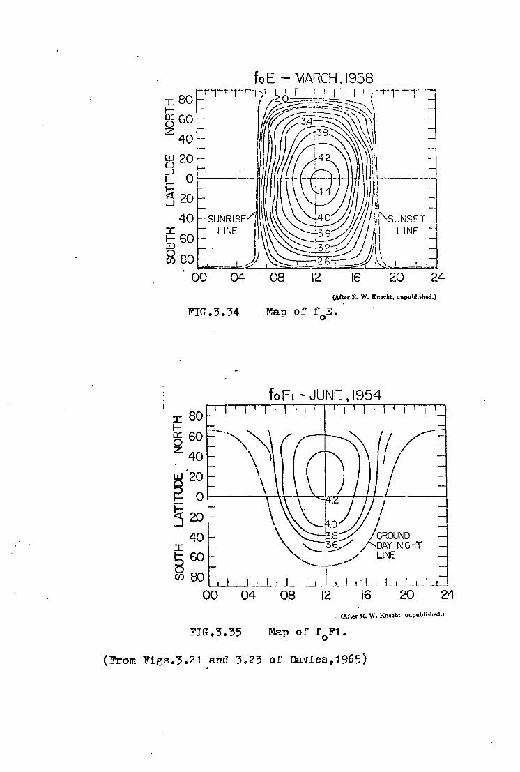
(After R. W. Knecht, unpublished.)
FIG.3.34
foF1 - JUNt., 1954
, (After R. W. Knecht, unpubli•hed.)
FIG.3.35 Map of :f0F1.
(From Figs.3.21 and 3.23 of Davies,1965) .
invoking the tilt model used by Papagiannis. For this model
the Z ray is a normally incident ray and should be treated
as such. Thus terms such as cos2 Bz and sin2 8z should be
omitted in the derivation, leading to the deletion of the
sin2W term from Eqn.3.1. When this is done and the
numerical example recalculated the "near-perfect numerical
agreement" comes even closer to perfection.
C) Papagiannis correctly states that Equation 3.1
" •••• shows that as we advance towards the equator, the angle
°"decreases whereas the angle (90-£tJ) increases. This makes
the appearance of the Z-mode echoes progressively more
" difficult, which is also borne out by observations. He
omits to point out that as we approach high latitudes the I I
angletx increases whereas the angle (90-w) decreases making
the appearance of Z-mode echoes progressively more
diffir.ult, which is not borne out by observations as the Z
echo is mainly a mid to high latitude phenomenon. For
instance, consider Macquarie Island which has a nigh
incidence of Z echoes and a dip angle of 78°. Substituting
this dip angle into Papagiannis's simple relation between°'
and W (Eqn.3.2) we obtain an value of around 25°, just
twice the required angle for Z ray return.
D) Papagiannis claimed that "ronograms which yield
values of the cyclotron frequency higher than those actually ..
present are a clear indication of d NS gradient..... and
"Ionograms in which tne Z mode appears (Meek,1948;
Newstead,1948) yield in general, increased values of the
local cyclotron frequency." Meek ann Newstead show only one
ionogram each. Meek makes no comment on the cyclotron
frequency. Newstead commented that he regularly found the Z
mode critical frequency to be higher than he expected. If
the gyro frequency is to be taken as the difference between
the X mode and Z mode critical frequencies, as is commonly
done, then it would appear from Newstead's expectations that
his ionograms yield decreased values of the gyro frequency.
Papagiannis suggests calculating the gyro frequency from the
0 and X mode critical frequencies but furnishes no evidence
or arguments to support his contention that Z mode ionograms
generally indicate N-S gradients.
Ellis (1957) has looked into this question with the
requisite thoroughness but as his calculations and theory
are based on his backscattering mechanism of return of the Z
ray his results may not be directly used as evidence for or
against the Papagiannis tilt model without reanalysis of the
observational data. We shall look at Ellis's (1957) results
more closely in Section 3.10.
E) The tilted layer ionosphere model of Papagiannis
takes into account the zenith angle of the sun but appears
to ignore the azimuth angle. However, since the Z ray must
(at least up to t~e coupling level) travel within the
magnetic meridian plane in all but the most exceptional and
unlikely circumstances, the azimuth angle of the the sun is
of crucial importance to the success or otherwise of this
model. Papagiannis has considered the N-S gradients caused
by the latitudinal change in the sun's zenith angle without
·taking into account the inseparably concomitant and
comparable magnitude E-W gradients caused by the
longitudinal change in the sun's zenith angle. Curiously
enough when discussing evidence for norizontal electron
density gradients, Papagiannis states "steep EW gradients
are almost always observed near sunrise and sunset at low
and mid-latitudes (HUGUENIN and PAPAGIANNIS,1965)." and near
sunrise is where Eowman (19B0) found the peak occurrence of
the Z echo at Hobart with a second smaller peak towards
sunset.
The tilt model proposed by Papagiannis will work only
when the sun's rays lie in the magnetic meridian plane.
Give that the declination at; Hobart is about 13°E and the
longitude 14?.5°E (time zone based on 150°Fi) one would
expect to see Z mode occurring most frequently on the 1100,
1115 and 1130 hrs. LMT ionograms if this theory is correct; (
not 1 in the afternoon as indicatea by Papagiannis when
applying his theory to Hobart. If we alter the time of day
to late morning we can assume the zenith angle of the sun to
be about 50° and substitution into Eqn.3.1 \
giv~s us an
·- ;/ £ _ _,:,./ ,..?:;..;--:,,/ .-~
b 15 5 0 0 ~ 5'0 answer of a out • rather than the required 18 ±1t1. • ,.
The time of day (early afternoon) chosen by Papagiannis when
substituting the parameters appropriate to Ellis's
observations into his equation is not the time of day when
Ellis reported recording Z echoes. Ellis (1953b) states "In
all cases tne observations were made bet~een 1500 and 1800
hours L.M.T. • • • 9 • • Ellis (1956) tabulates his results and
by weighting the observation times by the appropriate number
of observations we find that the average time of observation
is 1646 hours LMT, all observations occurring between 1500
and 1800 hours. An equinox zenith angle (although some
results are from winter months whicn would increase the
zenith angle) more appropriate to this time of day would be
about 80° and sustituting this into Eqn.3.1 we find thatoc: 0 now has a value of 31 which is far too large an answer. An
0 equinox zenith angle of 60 as used by Papagiannis
corresponds to about 1400 hours which is an hour earlier
than the earliest of Ellis's publisned observations.
It can be seen from the points raised that not only has
Papagiannis's tilt model been applied at a time other than when
the sun's rays lie in the magnetic meridian but also that the
"near perfect numerical agreement" vanishes when we substitute
a solar zenith angle more appropriate to the actual conditions
of Ellis's observations. Nevertheless, despite the
demonstrated snortcomings, it is an interesting idea and it is
worth examinin~ whether it mignt not have some relevance if
correctly applied. Ionospheric stations Hobart, Macquarie
Island and Brisbane are the locations wnich will be considered
for application of the solar zenith angle tilt model.
Transforming Eqn.3.1 we exp re s s i on f o r X
X = arc .tan[ R
H.tan3w
3.3
from which we can calculate the solar zenith angle required to
produce thee:< appropriate to the dip angle of tlie location in
question. Tabulating the required results for various Y
values at the three stations we have
STATION/(W) y = 1/6 1/3 1/2 2/3
MACQUARIE I./(78°) 1.. = 19° 25° 29° ~2 0
HOBART/ ( 72°) 'X = 51° 59° 63° 0
f'6
BRISBANE/(57°) J. = 85° 86° 87" 87°
We see that Z mode echoes at Brisbane would be expected
shortly after dawn and shortly before sunrise. As the
declination at Brisbane is about 10°E the sun's rays lie
nowhere near the magnetic meridian at these times and we would
not expect this mechanism to be responsible for any Z echoes at
Brisbane. An examination of world maps of magnetic dip and
declination show that this mechanism could not produce Z echoes
at any time of the day at any time of the yPar over quite a
large area of the earth including all locations of less than
30° geographic latitude. This automatically excludes the
. mechanism operating at all at many places where the Z moae is a
well known, if relatively infrequent, occurr~nce such as
Brisbane (Bowman,1960) and India (Toshniwal,1935; Banerji,1952;
Satyanarayana et al.,1959). Consider now high latitude
stations where the Z mode is a well known and relatively
frequent occurrence, such as Macquarie Island. Macquarie
Island's declination is 27°E and its minimum solar zenith angle 0 of 31 occurs at noon, summer solstice. The tabulated results
indicate that this mechanism could be responsible for Macquarie
Island Z echoes only at frequencies no higher than 2 MHz at mid
to late morning at summer solstice. Fig.3.36 is an excellent
example of Z echo at F2 frequencies at Macquarie Island.
Figs.3.20 and 3.22 show the 1951 diurnal and 1953 seasonal
variation of Macquarie Island Z echo. This mechanism is
clearly unable to account for Macquarie Island Z echo
occurrence. The Z echo also occurs relatively frequently at
Hobart whose latitude falls between that of Brisbane and
Macquarie Island. Papagiannis's solar zenith angle tilt
mechanism can probably provide Z echo at Hobart for about half
the year but only at one particular frequency on any ·given day
and only at about 1115 hours LMT. The approximate annual
variation of the allowed frequency is plotted in Fig.3.37.
Reference to Figs.3.20,3.22 and published Hobart ionograms
(e.g. Newstead,1948; Bowman,1960) will respectively show a
morpholo~y of the Hobart Z echoes and actual examples which
cannot be explained by this tilt mechanism.
Clearly then, even if this mechanism were to function
adequately in the F2 region (which is unlikely) it is of such
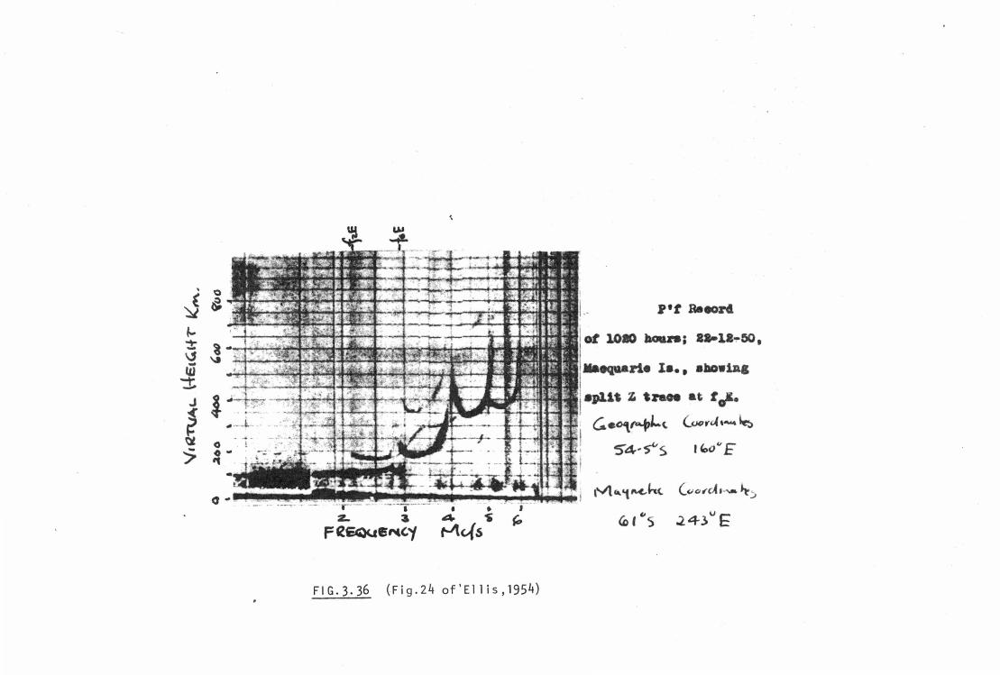
0 1 ~~~~~ 1r::t-t~-:-¥...,..;;.t-~~---~H-,l~~.uli
FI G. 3. 36 (Fi g . 2 4 of ' E 1 1 i s , 19 5 4)
R't a.eon
ot 10ao boun; aa-11,.50,
.lllaeqwaJi• la., abowiag
j •pll' Z 'n" at t~.
G.•04\~L(. (uor-d ,_ ~
I ~o" E
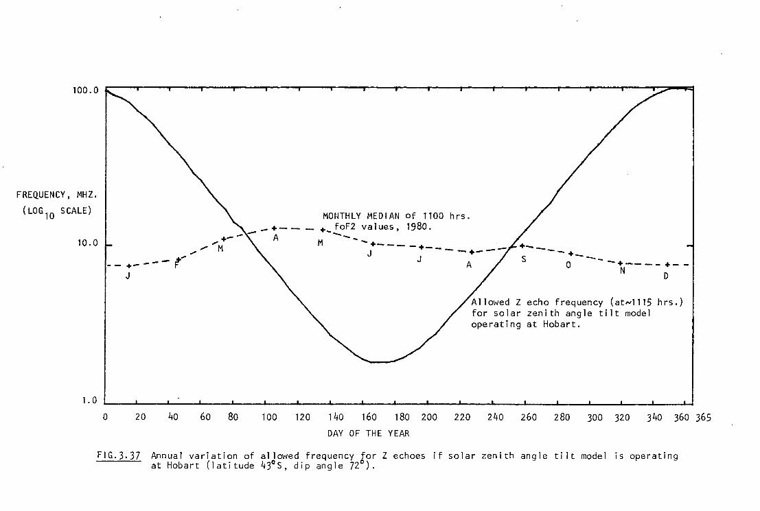
100.0
FREQUENCY, MHZ.
(LOG 10 SCALE)
10.0
1. 0
0
-+- -J
F ...
20 40
..... +
,,.,... ,....M
60 80
-+-- -A
100 120
MONTHLY MEDIAN of 1100 hrs. + foF2 values, 1980. .. _ M -- -+--- -+--
J - --+---J
A
140 160 180 200 220
DAY OF THE YEAR
0 -- -+---- +- -N
D
echo frequency (atN1115 hrs.) for solar zenith angle tilt model operating at Hobart.
240 260 280 300 320 340 360 365
FIG.3.37 Annual variation of al lowed frequency for Z echoes if solar zenith angle tilt model is operating at Hobart (latitude 43°5, dip angle 72°).
limited application that it would be a highly optimistic
estimate which would allow it to account for even one percent
of global Z echo occurrences. Since the electron density
profile model used by Papagiannis is known to be a generally
inadequate model for the F2 layer, it was thought worthwhile to
examine world FoF2 maps with a view to establishing wnet~er
favourable N-S tilts of the type proposed might be expected to
occur over Hobart, bearing in mintt that the
tilt would be required to be very small.
examined are shown in Figs.3.38 and 3.39.
magnetic east-west
Two of the maps
Upon superficial
examination a couple
suitable candidates
of regions
but a few
on the maps appeared to be
calculations based on the
separation and values of adjacent contour lines demonstrated
that there would need to be completely unrealistic variations
in height with latitude of t~e various plasma frequency levels
in order to provide the needed tilts.
Papagiannis's proposal for
theory by a system of sounders
experimental testing of his
located along the magnetic
meridian would have some problems in tnat in tae presence of
the Z echo returned by his tilt mechanism the sounders would no
longer be sounding overhead nor would his sounders remain
interlaced by deflection of 0 and X modes. T~e situation would
be practically the same as sounding a plane horizontally
stratified ionosphere at the dip pole with the main difference
being that the ground plane would,not be parallel to the
ionosphere. This difference does not alter in any way the
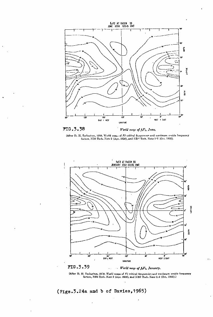
:' ;
lol'
~ !I" ~
;oo
:;:
60'
!AST I UST l(ST I UST lO•CllUll!
FIG.3.38 World map of foF:, June.
(Altrr D. II. Znch,.ri-cn, 1959, Worlcl mBJ;• of F2 criti<·nl fr.:<1m·n~1r• &.nd m:,.imum ll't•l.Jle lrcqucncy l:•ck.-. ~1!3S Ted•. ;\;otr 2 (Apr. 19.)9), and ~•Ii~ 'l'•ch. Note '.!.12 \O<t. 19C.O).
foF2 AT RASSN SO ..--~-.--~---.~~~~,.--J_A_NU~A_Rf~l2~CO...--r.o_u_~s~c_M_T~-.--~-.-~-..,,--~-.-~-,~·
ill'
JO'
o•
'llJ'
IO'L-~--L~~~~L,~~.1-.~-l~lu-,~---'~~-llLQ'~~...J,__~~LIO',...-~-'-~~Lt~~...L.-~~~'
[ISi ! IUI llSI j !AST LOICllUD!
FIG.3.39 · • World map of Jr;F., January.
E
0
(After D. JI, Zo.chariscn, 19;,9, Worl<I map• of F2 critic1<l frequcncic• and nio.•imum U•llbl• fr.-quenCJ' factor., NUS Tech. Note 2 (Apr. 19.59), and NBS T<..:h. Note :i,2 (Oct. 19l;()),)
(Figs.3.24a ~nd b of Davies,1·965)
results which would be obtained by a receiver/transmitter
ionosonde. A much simpler and less ambiguous test would be to
measure the angle of arrival of the Z echo. This is precisely
what Ellis did and as previously stated he found the angle of
arrival of the Z echo to be consistently about 9°N of zenith
and in the magnetic meridian. Ellis observed no angles of
arrival at or near 18°N of zenith, the angle predicted by
Pa~agiannis's solar zenith angle tilt model.
If a detailed global study of the occurrence of the Z echo
were undertaken it would be interesting to calculate the times,
days and frequencies for which Papagiannis's model would be
expected to work in the E and Fl regions at the various
locations and to see if any increased occurrence of Z echo
occurred under these conditions. The varied range of
declination and dip values found at a given geographic latitude
would facilitate the isolation of this effect.
3.9 Return Of The Z Ray - Papagiannis And Miller
Papagiannis and Miller (1969) discussed Ellis's postulate
of strong backscattering at the reflection level. Tney stated 0
PITTEWAY(1959) objects to this scheme on the grounds that
backscattering would not be sufficiently large at a level where
the i~dex of refraction is much smaller t~an unity" and
considered another difficulty with the backscatterin~ to be
•.•• the fact that Z-mode echoes are received over a fairly
wide range ( 1 MHz) of transmitted frequencies. Tnis implies
that conditions of strong backscattering also exist at lower
heights heights, while Z-mode echoes of higher frequencies
appear to propagate undisturbed in tbese regions." They then
proposed the alternative explanation of a favourable tilting of
t~e ionospheric layers, stating that "BOWMAN(1960), on a basis
of experimental observations, and PAPAGIANNIS(1965), on the
basis of a theoretical analysis have shown independently that
tnis could be the mechanism which allows the return of the
Z-mode echoes. Supporting evidence of this mechanism also
comes from the fact that ionograms containing Z-mode echoes
generally show a tilting of the ionospheric layers toward the
equator (MEEK,1948; NEWSTEAD,1948; ELLIS,1957)." They
considered that Ellis's (1957) analysis (for horizontal
gradients) of Z echo ionograms and implied that the presence of
measurable gradients supported the tilt theory.
Papagiannis and Miller then ray traced the
variety of tilted layer configurations of the
order to obtain actual supporting evidence
Z-mode in a
ionosphere in
for tne tilt
mechanism. As coupling regions are not a~enable to ray tracing
techniques they incorporated the qualitqtive effects of the
coupling cone by skipping the coupling zone in the ray tracing
and simply continuing the rays from the two boundaries of the
zone, using the chosen coupling angle f-'~ as the starting angle
~· They developed a method for choosing tne boundaries of the
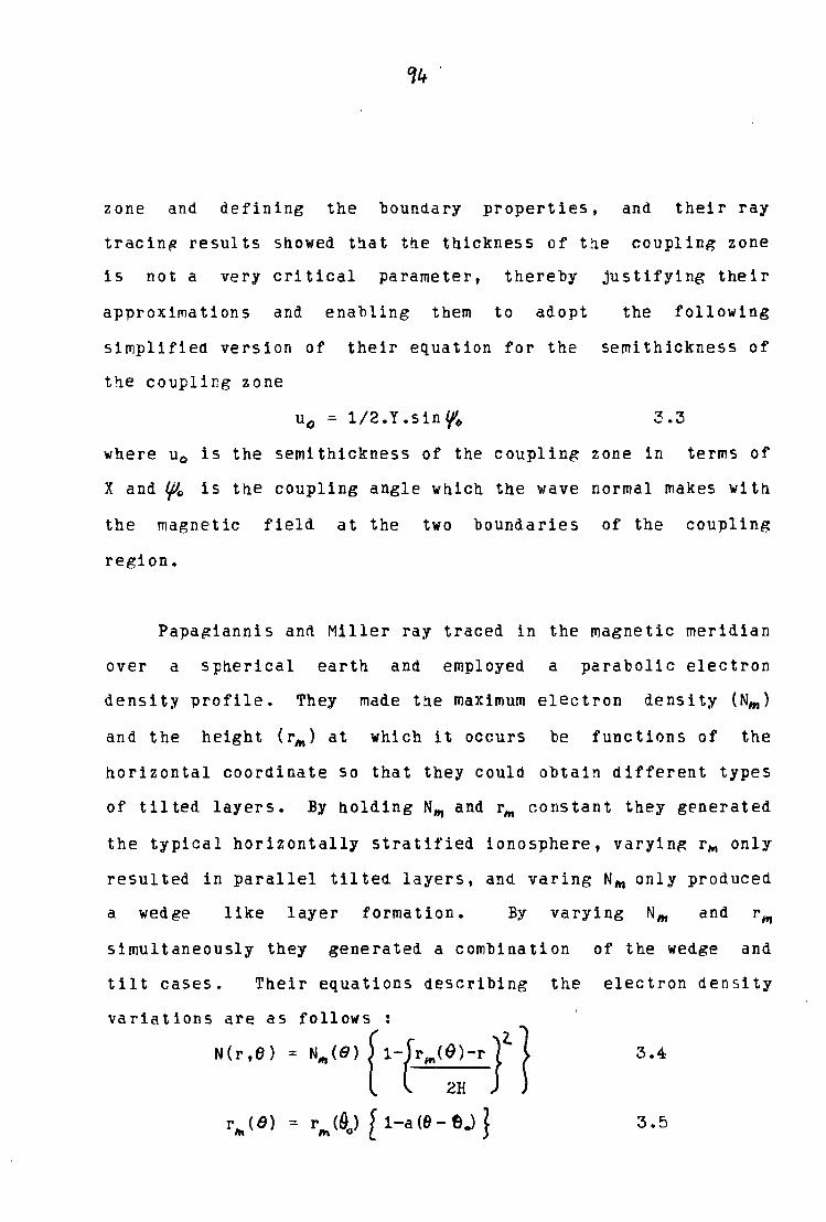
'll+ '
zone and defining the boundary properties, and their ray
tracin~ results showed that tne thickness of t~e coupling zone
is not a very critical parameter, thereby justifying their
approximations and enabling them to adopt the following
simplified version of their equation for the semithickness of
the coupling zone
3.3
where u0 is the semithickness of the coupling zone in terms of
X and f./1o is the coupling angle which the wave normal makes witn
the magnetic field at the two boundaries of the coupling
region.
Papa~iannis and Miller ray traced in the magnetic meridian
over a spherical earth and employed a parabolic electron
density profile. They made the maximum electron density (N~)
and the height (rm) at which it occurs be functions of the
horizontal coordinate so that they could obtain different types
of tilted layers. By holding N~ and rm constant they generated
the typical horizontally stratified ionosphere, varyin~ r~ only
resulted in parallel tilted layers, and varing NM only produced
a wedge like layer formation. By varying N,,,
simultaneously they generated a combination of the wedge and
tilt cases. Their equations describing the electron density
variations are as follows :
N ( r , B ) = N~ ( 6 ) f 1-r: r'" ( :~ -r r } 3.4
r"' (8) = rm a}0 ) [ 1-a (B- f>o) l 3.5
N,..(9) = N,,,( 90 ){ 1+b.r,,,( 60»(9-90 ) }
zhl(0)
The values they substituted in the above
R =6375km; 0
3.6
formulae were
e =33 "; ()
H=50km. For tne Earth's magneti~ field they used the standard
dipole approximation.
They ray traced from X = 1 with the wave normal parallel
to the magnetic field or from X = 1+u0 with the wave normal at
an angle (/10 to the magnetic field. They also traced the Z mode
downwards from X = 1 or X = 1-u 0 in order to establish the
location of the transmitter at the ground level. They adjusted
the ray tracing starting point along the X = 1 line in order to
make rays of all frequencies have a common transmitting point
at ground level.
Using a variety of values for the parameters a and b
(which define the tilting of the layers), Papagiannis and
Miller ray traced for possible Z mode returns. It is worth
quoting their results and conclusions as reported in their
paper.
"when a=b=0, no ray can return to the ground. When b=0
but a#0, i.e. in the case of paralell tilted layers. there is
-generally no ray of any frequency that can return to the
ground; however, in the particular case when the layers are
tilted at right angles to the magnetic field, i.e. when a=cotw,
where W is the aip angle of the magnetic field, the rays of
practically all the frequencies return to the ground
(Fig.3.40). This is almost identical to vertical propagation
with a vertical magnetic field in a horizontally stratified
ionosphere.
"on the other hand, when a=0, but b/0, i.e. in the case of
a wedge-like layer formation, if b is within reasonable limits,
there is a single ray, corresponding to a particular frequency,
that returns to the ground, but rays of adjacent frequencies do
not return (Fig.3.41). Actually one can obtain the return of a
very narrow spectrum of rays, instead of a single ray, if the
effect of the coupling cone at X = 1 is allowed for. In the
more realistic case of a10 and b~0, i.e. with layers that are
tilted both with respect to the horizontal and to each other,
we find that rays from a small range of frequencies ~0.1 MHz)
can return {Fig.3.42). When the effect of the coupling cone at
X = 1 is taken into consideration, the range of frequencies
over which rays may return to the ground is substantially
increased {Fig.3.43). In conclusion, when b tends to zero and
a to cotW the spectral range of the Z mode echoes becomes very
wide, whereas, when a tends to zero and b to some reasonable
value it becomes very narrow; one can, therefore, expect to
find some intermediate values of a and b which will allow the
return of Z-mode echoes over a given spectral range.
"This is very nicely demonstrated in the ionograms of
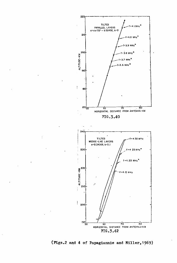
::.<; ::.:: I
w 0 ::> t-
5
210
~00
ct 190
180
230
:E 220 ~ I w 0 ::> t-
5 ct
210
200
TILTED PARALLEL LAYERS
o•cot72° • 0324192, b=O
60 70 BO
HORIZONTAL DISTANCE FROM ANTENNA-KM
FIG.3.40
TILTED WEOGE-LIKE LAYERS
o~0.24369, b=O.I
-t=4 30 Ml-lz
f•4.20 MHz,.
·-·f = 4 15 :VHz
r'
!9Q,_ _____ , ______ ,__ ____ 1 __ _
50 60 10 eo HORIZONTAL DISTANCE FRC'M ANTENN~-KM
FIG.3.42
(Figs.2 and 4 of Papagiannis and Miller,1~69)
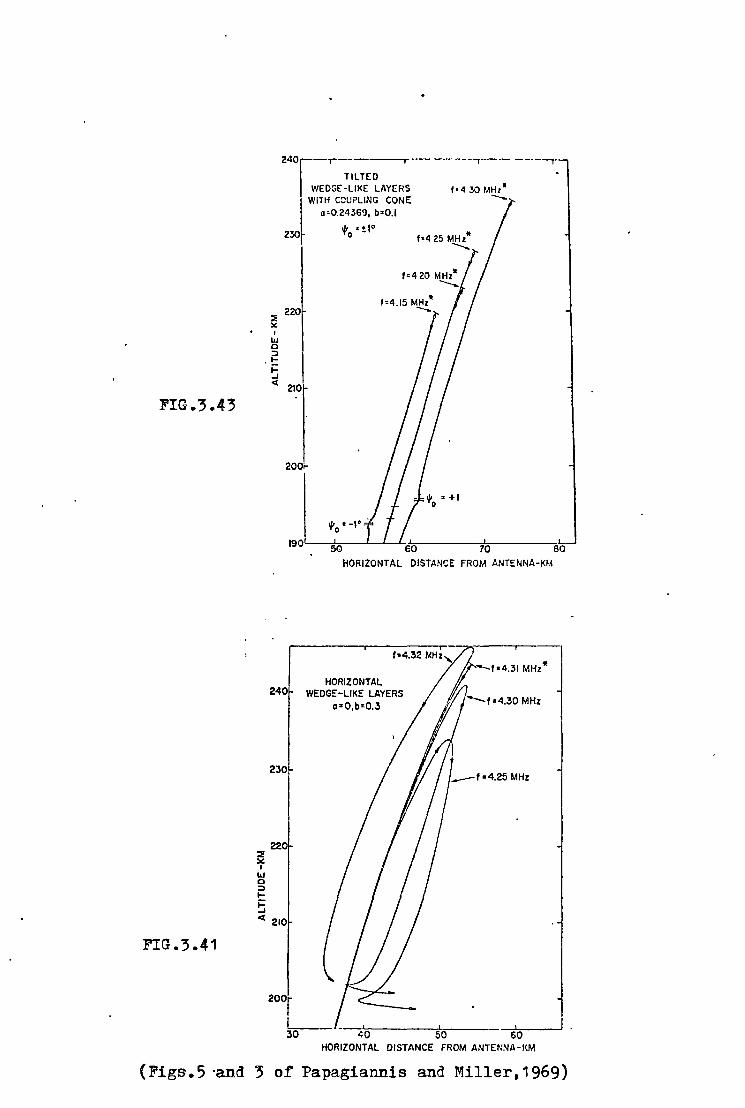
FIG.3.43
FIG.3.41
240 -.-------.--------,--·- -----,-
TILTED WEDGE-LIKE LAYERS
WITH COUPLING CONE a •0.24369, b•O.I
230 'fo •!lo
t/to • -1•
HORIZONTAL DISTANCE FROM ANTENNA-KM
-r•4.31 MHz* HORIZONTAL
240 WEDGE-LIKE LAYERS
a•O,b•0.3
230
220 ~ x I
Ill 0 :::> .... 5 <( 210
200
30 <O 50 60 HORIZONTAL DISTANCE FROM ANTEN:-.IA-KM
(Figs.5 ·and 3 of Papagiannis and Miller,1969)
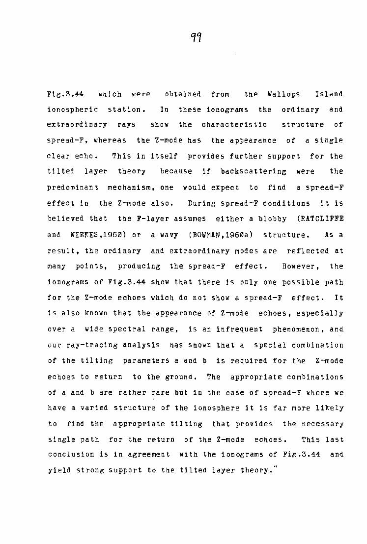
Fig.3.44 which were obtained from the Wallops Island
ionospheric station. In these ionograms the ordinary and
extraordinary rays show the characteristic structure of
spread-F, whereas the Z-mode has the appearance of a single
clear echo. This in itself provides further support frir the
tilted layer theory because if backscattering were the
predominant mechanism, one would expect to find a spread-F
effect in the Z-mode also. During spread-F conditions it is
believed that the F-layer assumes either a blobby (RATCLIFFE
and WEEKES,1960) or a wavy (BOWMAN,1960a) structure. As a
result, the ordinary and extraordinary modes are reflected at
many points, producing the spread-F effect. However, the
ionograms of Fig.3.44 show that there is only one possible path
for the Z-mode echoes which do not show a spread-F effect. It
is also known that the appearance of Z-mode echoes, especially
over a wide spectral range, is an infrequent phenomenon, and
our ray-tracing analysis has shown that a special combination
of the tilting parameters a and b is required for the Z-mode
echoes to return to the ground. The appropriate combinations
of a and b are rather rare but in the case of spread-F where we
have a varied structure of the ionosphere it is far more likely
to find the appropriate tilting that provides the necessary
single path for the return of tne Z-mode echoes. This last
conclusion is in agreement with the ionograms of Fig.3.44 and
yield strong support to the tilted layer theory.
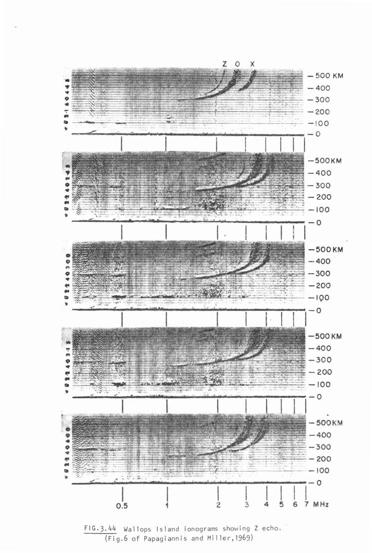
• •
.. .. ~
r.
• .. .. • • :... ~ .. • ~
• CJ ,, 9 .. ~
-500 KM
-400
-300
-200
-500KM
-400
-300
-200
-100
-500KM
-400
-300
-200
-100
-500KM
~~~•-400
I I 0.5 1
FIG.3.44 Wallops Island ionograms showing Z echo. (Fig.6 of Papagiannis and Miller, 1969)
-300
-5001\M
-400
/01
3.10 Critical Discussion
Papagiannis and Miller, through their ray tracing and
definition of appropriate electron density profiles, have
provided us with a satisfactory, well explored model for the
tilt mechanism of return of the Z ray. They have recognized
the need to confine the Z mode within the magnetic meridian
plane and have established the conditions under which a
reasonable range of Z mode frequencies would be returned. This
is the model by which the tilt mechanism should be judged. The
ray tracing method uses well accepted techniques (i.e.
numerical integration of Haselgrove differential ray equations)
and their clever, innovative method of skipping tne coupling
region appears from their reported results to be eminently
satisfactory for their particular application. Where
comparison is appropriate, the behaviour of their Z rays
appears to be in general agreement with the ray tracing of
Lockwood (1962). While there are no apparent difficulties with
their model and results, some objections could be raised when
considering their general discusion of the problem and the
conclusions drawn from their results. These are as follows
A) The
theoretical
experimental
results of
results of Bowman (1960)
Papaagiannis (1965) do
and
not
demonstrate that the tilt mechanism is a likely contender to
produce Z echoes, as has been shown by the discussion in
Sections 3.6 and 3.8. Although it has been shown to be a
/02
possible Z ray return mechanism it has not been established
that it is likely.
B) Pitteway (1959) did not specifically reference
Ellis's Z mode return mechanism and his work is not
exhaustive of backscattering possibilities, as discussed in
Section 3.4. Papagiannis and Miller's comment perhaps
follows the lead given by Ratcliffe (1959) in his discussion
of the Z mode. Ratcliffe states (p.129) "If, however, there
are irregularities in the electron distribution near the
level where X = l+Y, where )A' (real part of refractive index)
is small, there will be strongf backwards scattering and an
appreciable part of the energy will return along the
incident path." to which he adds the footnote '' tMore recent
work (Pitteway,1958) seems to indicate, however that
backscattering would not be
was small."
accentuatPd at a level w~ere/
Establishing that a proposed scattering resonance
(Booker,1955) would be suppressed because of the expected
collision frequency is quite another matter to establishing
that no backscattering mec~anism can give rise to the Z
echo. Ellis did not propose a scattering reso~ance and, as
discussed, if Briggs and Phillips (1950) scintillation
irregularities could produce spread-Fas postulated by Renau
then there is no reason why sufficient Z mode energy might
not be reflected back along the incident path.
/03
C) The claim that ionograms containing Z mode ecnoes
generally show a tilting of the ionospheric layers was made
previously by Papagiannis (1965) and has been discussed in
Section 3.8. Again no direct evidence or analysis of
ionograms is given in support of this contention.
and Miller claim that Ellis's (1957) results
tilt proposal and further claim that the 5
Papagiannis
support their
" examples out of 23 which do not support it •.• are propbably
the result of small {less than 1 per cent) reading errors of
the critical frequencies from the ionograms." They s~ow how
a small chanRe in the critical frequencies can alter a large
negative horizontal gradient to a positive gradient. They
do not state why the 18 cases of positive gradient should
not turn out to be large negative horizontal gradients as a
result of small reading errors of the critical frequencies.
As already pointed out in Section 3.8, Ellis (1957) analysed
the ionograms on the assumption that the Z echo was
occurring in an essentially flat ionosphereand his equations
must be radically altered if they are to be applied to the
tilt/wedRe model of Papagiannis and Miller. Until
Papagiannis and Miller reanalyse these or similar ionograms
taking tilts into account they cannot conclude whether or
not such ionograms support the tilt theory. As a matter of
interest, it is worth examining the ma~nitude of the tilts
which might be represented by the horizontal electron
density gradients deduced by Ellis. As a first
!Oft
approximation it shall be assumed that the peak height of
the layer is constant and that the electron density varies
parabolically as assumed by Papagiannis and Miller. The
expression for electron density is then
N(x,h) = N'"(x) { lt::h r} 3.7
Nm ( x ) = N"' ( x 0 ) + m * ( x -x 0 ) 3.8
where x is the horizontal coordinate in km., positive
towards the equator; h is the height in km. above the
Earth's surface; H is the scale height (=50km. as assumed by
Papagiannis and Miller); hm is the peak height as calculated
by Ellis; NM(x 0 ) is the overhead peak electron density as
calculated from the Z mode critical frequency of Ellis; m* _, is the horizontal electron density gradient in el/cc[km]
_, as calculated from the gradient m in c/s[km] deduced by
Ellis (m~ is positive for peak electron density increasing
towards the equator); p equals 2 or 3 for parabolic
ionospheres of semit~ickness 100 and 150 km. respectively;
x 0 is the horizontal coordinate of t~e Z mode reflection
point. We determine m~ from
milt = 2mf0
80.5
where f 0 is the 0 mode critical frequency, 1n MHz..
To determine the tilt of a layer of given electron
density Nx al:. a. given x coordinate
= canst.
we
Is
put N(x,h) = Nx
lo..f t:..l.<l. .a.:f t.d .f.to Yi'\ •
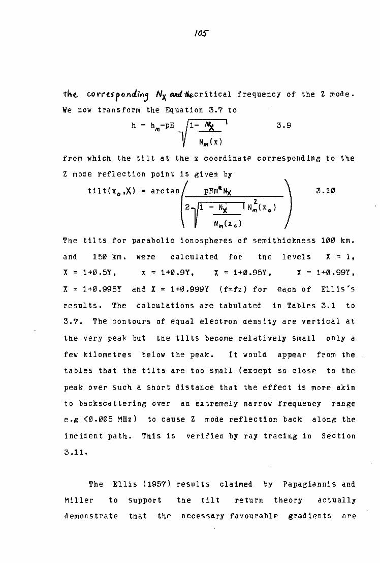
/OS
tht- C.OV't"tspon.cl.t"'j Nx "11ci-Hie.critical frequency of the Z mode.
We now transform the Equation 3.7 to
h = h111-pH-.~ v N1r1 ( x)
3.9
from which the tilt at the x coordinate corresponding to t~e
Z mode reflection point is given by
3.10
The tilts for parabolic ionospheres of semithickness 100 km.
and 150 km. were calculated for the levels x = 1,
X=1+0.5Y, x = 1+0.9Y, X = 1+0.95Y, X = 1+0.99Y,
X = 1+0.995Y and X = 1+0.999Y (f=fz) for each of Ellis's
results. The calculations are tabulated in Tables 3.1 to
3.7. The contours of equal electron density are vertical at
the very peak but tne tilts become relatively small only a
few kilometres below the peak. It would appear from the
tables that the tilts are too small (except so close to the
peak over such a Short distance that the effect is more akin
to backscattering over an extremely narrow frequency range
e.g (0.005 MHz) to cause Z mode reflection back along the
incident path. This is verifiea by ray tracing in Section
3 .11.
The Ellis (1957) results claimed by Papagiannis and
Miller to support the tilt return theory actuall~
demonstrate tnat the necessary favourable gradients are
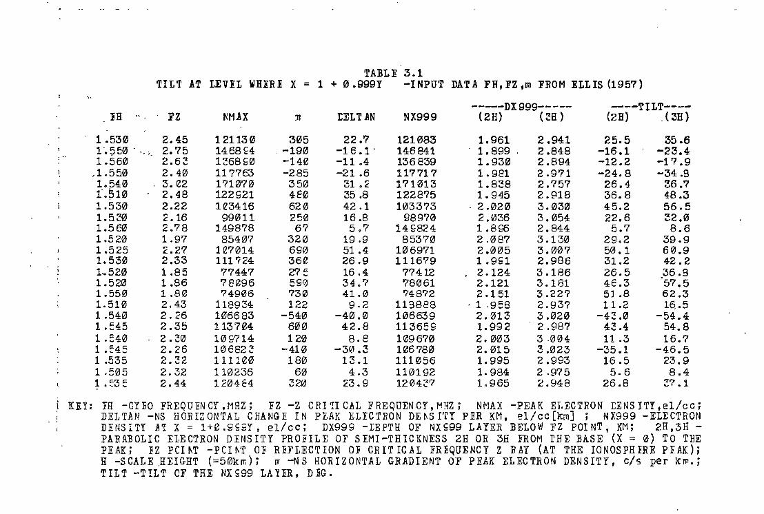
TA:BLE 3.1 TILT AT LEVEL WHER! X = 1 + 0.999Y -INPUT DATA FH,FZ,m FROM ELLIS (1957)
!H "' FZ
1 .530 1 ·• ~50 - ·- ;_ 1.560
.. 1.550 1 •. 540 f.~10 1.530 1.5~ 1.560 1.520 1.525 1.530 L520 1.520 1.550 1.510 1.540 1.:45 1 .!:40 1 .:45 1 .535 1 .505 1. ~3:
2.45 2. '75 2.6~ 2.40 3.e2 2.48 2 .22 2.16 2.78 1.97 2. 2'7 2.33 1.85 1.86 1.80 2.43 2.26 2.35 2. ::0 2.26 2. ::2 2.32 2.44
~MAX
121130 1468S4 1::68 S0 117763 171070 122921 1e3416
99011 149878
85407 1e7014 111'(24 77447 78096 74906
118934 106683 1137e4 109714 10682 ~ 1111e0 110236 1204E4
:n
305 '-190 -14~ -285 350 4E0 620 250 67
320 690 36e 275 590 ?30 122
-540 600 120
-410 180
60 320
tELTAN
22 .7 -1e.1· -11 .4 -21 .6
31 • 2 35.8 42.1 16.8 5.7
19.9 51 .4 26.9 16 .4 34.7 41.0 9-2
-40.0 42.8 8.8
-30 .3 13.1
4.3 23. g
NX999
121083 146841 136839 117717 171013 1228?5 103373
98970 14S824
85370 106971 1116?9
77412 78061 748?2
113888 106639 113659 109670 106780 111056 110192 1204~7
-----DX 999-- ---( 2 H) (~H)
1.961 1.899 1.930 1. 981 1.838 1. 945
. 2 .020 2 .036 1.896 2.087 2.005 1.9Sl 2.124 2.121 2 .151
, 1 -958 2.013 1.992 2. 003 2. 015 1.995 1. 984 1.965
2.941 2.848 2.894 2.971 2.757 2.918 3.030 3.054 2.844 3 .130 3 .007 2.986 3 .186 3 .181 3.227 2.937 3.020 2.987 3 .004 3.023 2.993 2 .975 2.948
---TILT----(2H) (3H)
25.5 -16.1 -12.2 -24.8 26.4 36.8 45.2 22.6 5.7
29.2 50. 1 31.2 26.5 4€.3 51 .8 11.2
-4:: .0 4:3.4 11 .3
-35.1 16.5 5.6
26.8
35.6 -2:3.4 -1? .9 -34 .s
36.'7 48.3 56.5 ~2.0 8.6
39.9 60.9 42 .2 36.9 ·57. 5 62.3 16. .5
-54.4 54.8 16.7
-46.5 23. 9 8.4
;:7 .1
KiY: IH -GYEO FREQUENCY.MHZ; IZ -z CRI~ICAL FREQUENCY,MHZ; NMAX -PEAK ELECTRON IENSITY,el/cc; DELTAN -NS HOBIZONTAL CHANGE IN PEAK ELECTRON DE~SITY PER KM, el/cc[km] ; NX999 -ELECTRON DENSITY AT x = 1+e.9SSY, el/cc; DX999 -rEPTH OF NXE99 LAYER BELOW FZ POINT, KM; 2H,3H -PARABOLIC ELECTRON DENSITY PROFILE OF SIMI-THICKNESS 2H OR 3H !ROM rHE BASE (X = 0) TO THE PEAK; :FZ PCI~T -PCI~T OJ REFLECTION OF CRITICAL FREQUENCY Z RAY (AT THE IONOSPHERE PF.AK); H -SCALE _HEIGHT (=50km); ~-NS HORIZONTAL GRADIENT OF PEAK ELECTRON DENSITY, c/s perk~.; TILT -TILT CF THE NXS99 LAYER, D:EG.
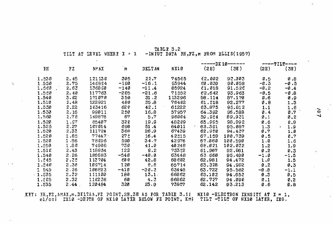
TA:BLE 3 .2 TILT AT LEVEL WHER:E x = 1 -INFUT DATA :FH,FZ,m FROM ELLIS(195?)
----DX 10------ ----TILT----!H FZ Nl"'AX m DELTAN NX10 (2H) ( 3H) (2H) ( 3H)
1.:30 2.45 121130 305 2:: .? ?45€5 E2.002 9~ .;:,03 0.5 0 .8 ', 1 .550 2.75 1468S4 -190 -16.1 S3944 e0 • 039 90.058 -0.3 -0 .5
1.5€0 2.6~ 1368 S0 -140 -11 .4 85924 El. 018 91.526 -0. 2 -0.4 1.550 2.40 117763 -285 -21 .6 71552 e2 .642 93 .963 -0.5 -0.8 1.540 3. !22 1?1070 350 31 .2 113296 58. 114 87 .170 0.6 0.9 1.510 ::.48 122921 480 35 .8 76402 61. =is 92.277 0.8 1.3 1.530 2.22 1e3416 62e. 42.1 61222 63.875 95. 812 1.1 1.6
' ....... 1.53il 2 .16 99011 250 16 .. 8 5795? 64.392 96.588 0.4 0.7 ()
1.500 L7E 149878 67 5.7 96004 59. 9=4 89. g ~1 0.1 0.2 --..l
1.520 1. S7 85407 32e 19.9 482e9 65.995 98.992 0.6 e.9 1.525 2.27 1!27014 690 51 .4 64011 63.391 95.08? 1.3 1.9 1.5~0 2.33 111724 360 26.9 67439 62.9E8 94.43? 0.7 1.0 1.!520 1.85 '7?447. 27= 16 .4 42515 6'7.159 100.739 0.5 e.7 1.520 1.86 78C/,96 590 34.? 42976 6? .060 100.590 1.0 1.6 1.!:50 1 .80 74906 '730 41.0 40248 6E. 0 21 102.032 1.2 1.9 1 .51 f: 2.43 118934 122 9.2 733!:2 61.907 92 .861 0.2 0.3 1.540 2.26 106683 -540 -40.0 63448 63.660 95 .490 -1.0 -1.5 1. !:45 - 2-~= 113 '(04 €00 42.8 68€02 62 .981 94.472 1-.0 1.5 1.!:40 2.30 109?14 120 8.8 65714 63. 328 94 .992 0.2 0.3 1 545 2-~6 106823 -410 -30.3 63448 63. 722 95. 582 -0 .8 -1.1
. 1. !:35 2.32 111100 180 13.1. 668€2 E3.102 94.653 0.3 0.5 1.!:C5 2.32 11e2~6 60 4.3 66862 62. 727 94.09ll 0.1 0.2 1.=35 2.44. 120484 320 23.9 ?39f:7 62 .142 93 .213 0.6 0.8
KIY: !H,FZ,h~AX,m,DILTA~,FZ POINT,2H,3H AS FOR TABLE 3.1; NX10 -ELECTRON IENSITY AT X = 1, el/cc; IX10 -DE FTH OF NX10 LAYER BELOW FZ POINT, KM; TILT -TILT OF NX10 LAYER, IEG.
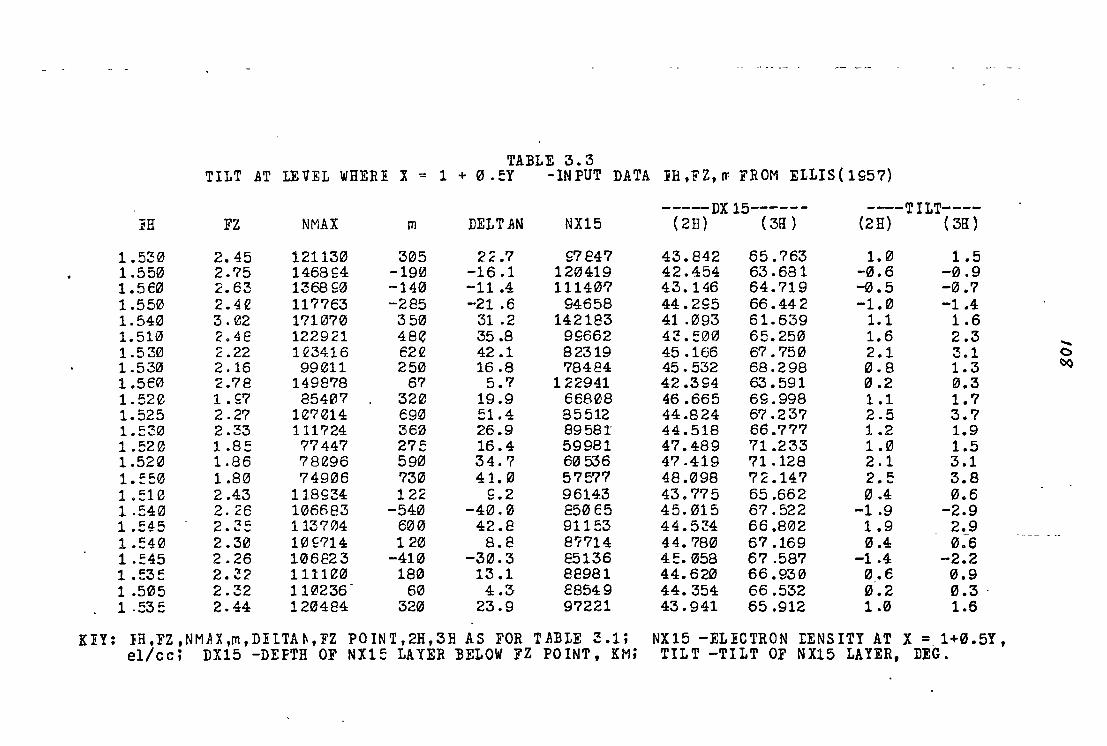
TABLE 3.3 TILT AT LEVEL WHER:E x = 1 + 0. eY -IN PUT DATA iH,FZ,~ FROM ELLIS{l957)
-----DX 15------ ---TILT----:rn FZ NMAX m DELT AN NX15 (2H) ( 3H) (2H) ( 3H)
1.5~0 2.45 121130 305 2;:. 7 S7S47 43.842 65.763 1.0 1.5 1.550 2.75 1468£4 -190 -16.1 120419 42.454 63. 681 -0.6 -0.9 1.5€0 2.63 1368 £0 -140 -11.4 11140'7 43.146 64.719 -0 .5 -0.7 1.550 2.4e 1177€3 -285 -21 .6 94658 44.2S5 66 .442 -1.0 -1.4 1.540 3. 02 171070 350 31 .2 142183 41 .093 61. 639 1.1 1.6 1.510 2.4E 122921 4Be 35.8 99662 4~.:00 65.250 1.6 2.3 -1.:130 2.22 1Q3416 62!2 42.1 82319 45 .166 67. 750 2.1 3.1 ()
1.530 2 .16 99011 250 16 .8 784E4 45. 532 68. 298 0.8 1.3 C)O
1.5€0 2.78 149878 67 5.7 122941 42 .3S4 63. 591 0.2 0.3 1.520 1. S7 85407 32'1l 19.9 66808 46 .665 69.998 1.1 1.7 1.525 2.27 1e7014 €90 !:1.4 85512 44 .824 67 .237 2.5 3.7 1. :'.30 2.33 111724 360 26.9 89581 44.518 66.777 1.2 1.9 1 .520 1 .BE 77447 275 16. 4 59981 47.489 71.233 1. 0 1.5 1.520 1.86 78e96 590 34.7 60536 47.419 71 .128 2.1 3.1 1.:50 1.80 74906 730 41. 0 57577 48.098 72.147 2.e 3.8 1.:10 2.43 118S34: 122 S.2 96143 43. 775 65.662 0 .4 0.6 1 .540 2.26 106683 -540 -40.0 E50e5 45.015 67. 522 -1.9 -2.9 1.!:45 2-~= 113704 600 42.8 91153 44. 5~4 66.802 1.9 2.9
---~- - --
1.!:40 2.30 10 S714 120 8.8 8?714 44. 780 67 .169 0.4 0.6 1 .!:45 2.26 106823 -410 -30.3 E5136 4!:. 058 67.587 -1.4 -2.2 1 .:3e 2.~2 l 11H~0 180 13.1 8S981 44. 620 66. 93 0 0,.€ 0.9 1 .505 2.32 110236 60 4.3 c8549 44.354 66.532 0.2 0.3 . 1 .535 2.44 120484 320 23.9 97221 43. 941 65.912 1.0 1.6
KIY: IH,FZ,NM~X,m,DilTA~,FZ POINT,2H,3H AS FOR TAELE ~.1; NX15 -ELICTRON IENSITY AT X =. 1+0.5Y, el/cci DX15 -DEFTH OF NX15 LAYER ~ELOW FZ POINT, KM; TILT -TILT OF NX15 LAYER, DEG.
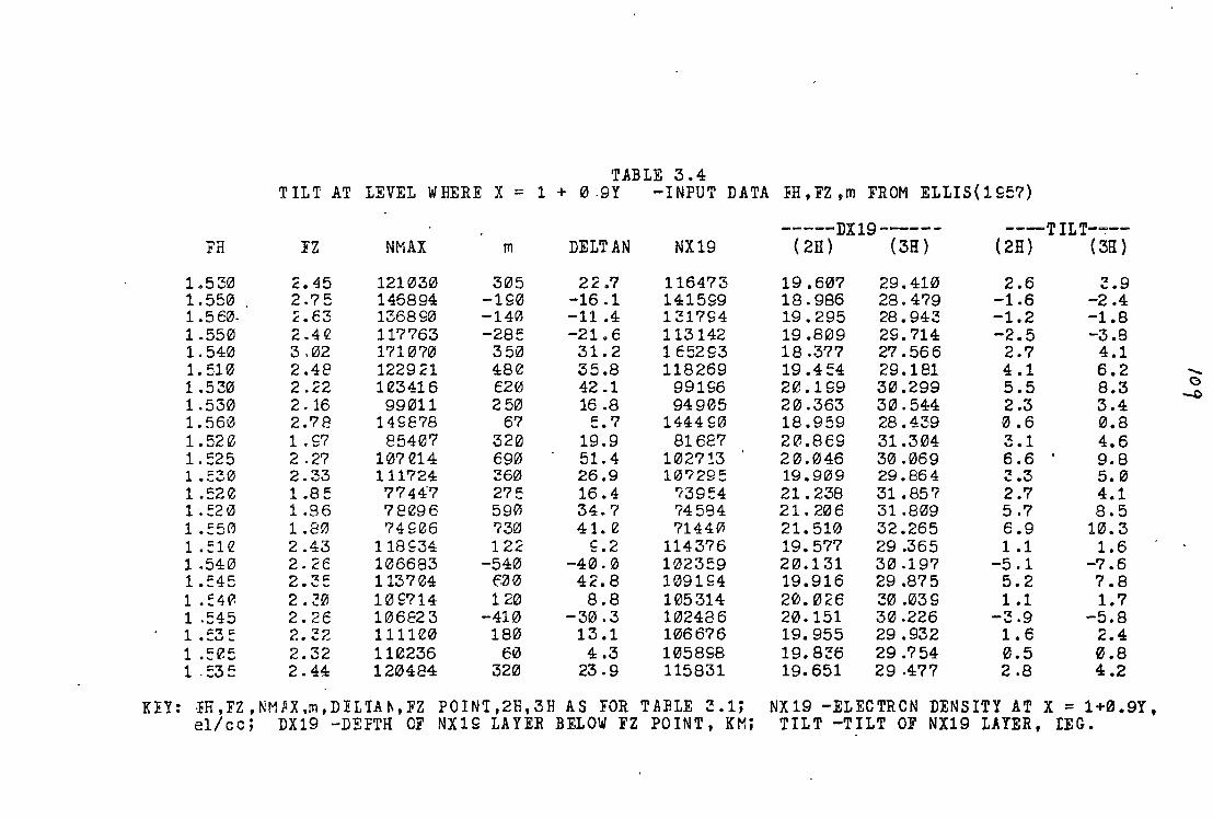
TABLE 3.4 T !LT AT LEVEL WHERE x = 1 + 0.9Y -INPUT DATA FH, FZ ,m FROM ELLIS{ 1 S57)
-----DX19------ ---T !LT--:'--FR rz NMAX m DELT AN NX19 (2H) (3H) (2H) (3H)
1.530 2.45 121030 305 22 .7 116473 19.607 29.410 2.6 ~.9 1.550 2.75 146894 -1S0 -16.1 141599 18. 986 28.479 -1.6 -2.4 1.5 E0- ~.€3 136890 -140 -11.4 131794 19. 295 28. 943 -1.2 -1.B 1.550 2 .4 e 117763 -28e -21. 6 113142 19.809 29.714 -2.5 -3.8 1.540 3.02 171070 350 31.2 1 €5293 18 .377 27. 566 2.7 4.1 1. 510 2.4E 122921 48e 35.8 118269 19 .4 !:4 29 .181 4.1 6.2 -1 .530 2.22 1e3415 €20 42.1 99196 20.199 30.299 5.5 8.3
<:)
-0 1.530 2 .16 99011 250 16 .8 94905 20 .363 30.544 2.3 3.4 1.560 2.7 e 14SE78 67 E.7 1444£0 18.959 28.439 0.6 0.8 1.52~ 1. S7 85407 320 19.9 81687 20.869 31.304 3.1 4.6 1.525 2 .27 107 e14 690 51.4 1027!3 20 .046 30 .069 6.6 . 9.8 1 . .:00 2.33 111724 360 26.9 107295 19. 909 29 .864 3.3 5.0 1 . 52 e 1 .8 = 7744·7 275 16. 4 '73954 21. 238 31. 857 2.7 4.1 1. :20 1 .86 781296 590 34.7 74584 21. 206 31.809 5.7 8.5 1 .:50 1.80 74Sl26 730 41. e 71440 21. 510 32.265 6.9 10.3 1 . : 1 e 2.43 118S34 122 f.2 114376 19.577 29 .365 1 .1 1.6 1.540 2.26 106683 -540 -40.0 1023!:9 20.131 30.197 -5.1 -7.6 1.:45 2.~: 1137e4 f.~0 42. 8 1091 S4 19.916 29 .875 5.2 7.8 1 . :40 2. 20 10 £714 120 8.8 105314 20.026 ~0 .039 1 .1 1.7 1 ,545 2.26 10682 3 -410 -30 .3 102486 20.151 30.226 -:3 .9 -5.8 1 .:3: 2. ::2 111Hrn 180 13.1 106676 19.955 29 .932 1.6 2.4 1 .:ee 2.32 110236 60 4.3 105898 19.8~6 29 .754 0.5 0.8 1 .:35 2.44 120484 320 23 .g 115831 19.651 29.477 2.8 4.2
K:EY: JH,FZ,NMflX,m,DliL~A~,FZ POIWI,2R,3H AS FOR TA]LE ~.1; NX19 -ELECTRCN DENSITY AT X = 1+0.9Y, el/cc; DX19 -DEFTH OF NX19 LAYER BELOW FZ POINT, KM; TILT -TILT OF NX19 LAYER, IEG.
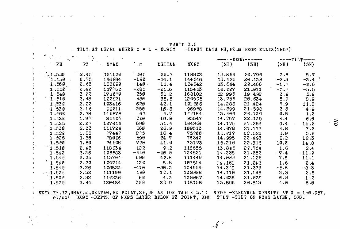
T A:BLE 3 .5 TILT. AT LEVEL WHERE X = 1 + 0.95Y -INPUT DATA FH,FZ,m FROM ELLIS(1957)
·' ; . ·.
----·-DX95----- ---TILT---FB FZ NMAX m DELTAN NX95 ( 2H) (3H) ( 2H) (3H)
.~:. 1-.530 2 .45 121130 . 30: 22.'7 118802 13 .864 20.796 3.8 5.7 ·" 1 ·• ·=50 2.75 146E94 -190 -16.1 144246 13.425 20 .138 -2.3 -3. 4:;
1 .E60 2. E3 136E90 -140. -11.4 134342 13.644 20.466 -1 .7 -2.6 1 -=5t 2.40 117?63 -285 -21.6 115453 14.007 21.011 -3.7 -5.5 1.E40 3.02 171€70 350 31.2 168182 12. 995 19 .492 3,9 :.9 1 .=10 2.48 122S21 480 35. 8 12059E 13. 756 20 .634 5.9 8.9
- 1 .::3 e 2.22 103416 620 42 .1 101206 14.283 21 .424 ?.9 11.8 1 .53 0 2 .1 e 99011 250 lp.8 96958 14. 399 21.598 ~-3 4.9 1 .::6e 2.78 149878 6'7 5.7 147184 13. 406 20 .109 0.8 1.2 1 .:2e 1.9? 8540? 320 19.9 83547 14. 757 22 .135 4.4 6.6 ....... 1 .!52!5 2.27 107014 690 51.4 1048€4 14.175 21 .262 9.4 14.0 -c 1 .!530 2.~3 111724 360 26.9 109510 14. 078 21.117 4.8 7.2 1 .e2e 1. 85 ?'7447 275 16.4 75700 1 =. 017 22 .526 3.9 5.9 1 .520 1. 86 780£6 590 34 .7 76340 14.995 22 ,493 e.2 12 .3 1.5!50 1.80 74 £06 7~0 41.0 73173 15.210 22.91!: 10.0 14.8
·- 1 .510 2.43 118£34 122 9.2 116655 13.843 2e .764 1.6 2.4 1 .540 2.26 106683 -5~0 -40 .0 104521 14 .235 21.352 -7.4 -11.0 1 .54 = 2.~5 113704 €00 4 '2 .8 111449 14. 08~ 21.12: 7.5 11.1 ,.
. 1. 540 2.~0 1e9?14 12e 8.8 107514 14 .161 21. 24-1 1.6 2.4 1.54: 2.26 Hrn823 -410 -30 .3 104654 14 .249 21. 373 -=.6 -8.3
:·• 1. 53: '-'.. 32 111100 180 1 ~ .1 1088E8 14. 110 21.165 2.3 2.5 1.50: 2.32 110236 60 4.3 108067 14. 026 21. 039 0.8 1.2 1.53: 2.44 120484 320 2~ ,g 118158 13 .895 20. 843 4.0 6.0
KEY-: FB,iZ,NMAX,~,DELTAN,FZ pc I f\ T '2 E I ~H AS FOR TA:ELE ~.1; NX9= -ELECTRCN DENSITY AT X = 1 +0 .95Y I
el/cc; DX9: -DEPTH OF NX95 LAYER ~ELOW FZ POINT, KM; TILT -TILT OF NX95 LAYER, DEG.
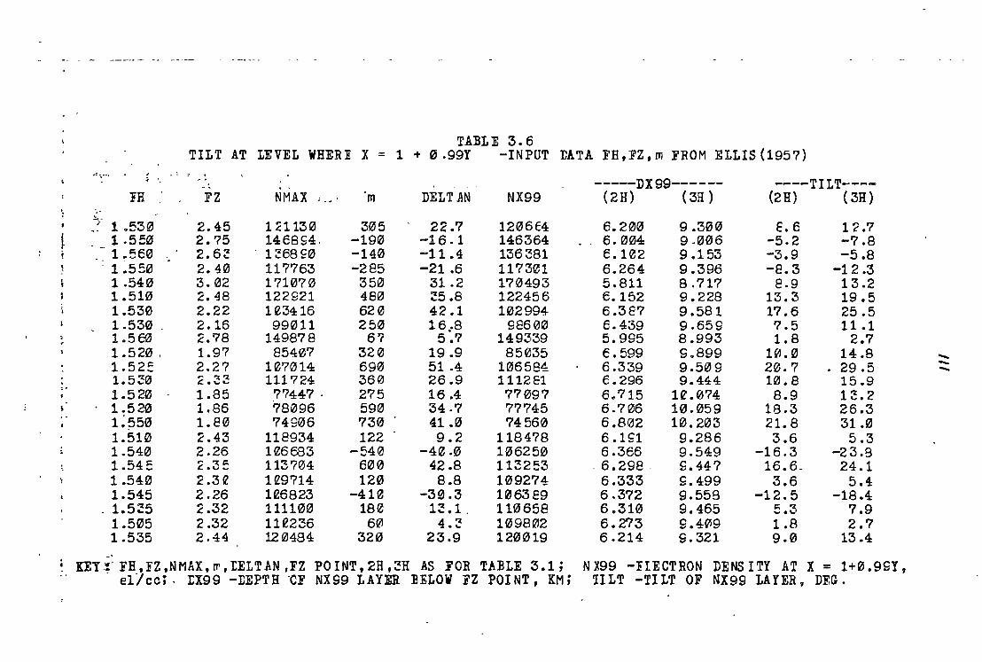
TABLE 3. 6 TILT AT LEVEL WEER I x = 1 + 0.99Y -INPUT tATA FB,FZ,m FROM ELLIS(1957)
~-= ••••· ' ' . 4 ·, -----DX99------ ----TILT----- ' ..
!H FZ NMAX .. , m DELT AN NX99 (2H) ( 3H) (2H) ( 3H)
. 1 .530 2.45 1 ~1130 305 22.7 1206€4 6.200 9.300 E.6 12 .7
i 1 .s=0 2.75 1468G4. -190 -16 .1 146364 6.004 9.006 -5.2 -7.8 1.560 ·. 2. 6~ 1 ~68 £0 -140 -11.4 136381 e.102 9 .153 -3.9 -5.8 1 .. 550 2. 40 117763 -285 -21 .6 117301 6.264 9.396 -8.3 -12 .3 1 .540 3. 02 171070 350 31.2 170493 5.811 8.717 e.g 13 .2 1.510 2. 48 122921 480 ~5.8 122456 6.152 9.228 13.3 19. 5 1.530 2.22 1'~34: 16 620 42.1 102994 6.3E7 9 .581 17.6 25.5 1.530 . 2.16 99011 250 16 .. 8 98600 6.439 9.659 '7. 5 11 .1 1.5E0 2.78 149878 6? 5.7 149339 5.995 8.993 1.8 2.7 1.520 . 1.97 85407 320 19.9 85035 e. 599 9.899 10.0 14.B -1.52e 2.27 107014 690 51.4 106584 6.339 9.509 20.7 29.5 --1.5~0 .. '2: '4
~ . ..., '- 111724 360 26.9 1112E1 e.296 9.444 10.8 15.9 ,. 1.520 1.85 _7'7447 . 275 • 16.4 77 097 6.715 1e.074 8.9 13. 2 1.520 1.86 78096 590 34.7 77745 6.706 10. 059 18.3 26.3 1~~50 i. e0 74906 730 41 .0 74560 6.802 10.203 21. 8 31.0 1.510 2.43 118934 122 9.2 118478 6.1£1 9.286 3.6 5.3 1.540 2.26 1e6683 -540 -4~ .0 106250 6.366 9.549 -16.3 -23.9 1.54:: 2 .3e 113704 600 42.8 113253 -6.298- 9.447 16.6- 24.1 1.540 2 .312 1fl9714 120 8.8 109274 6.333 9.499 3.6 5.4 1.545 2.26 1'~6823 -41~ -30 .3 1063E9 6.372 9.558 -12.5 -18.4
. 1.5~5 2.32 111100 180 1~.1 . 110658 6.310 9.465 5.3 7.9 1.505 2 .32 11e23s 60 4.~ 109802 6.273 9.409 1.8 2.7 1.535 2.44 120484 320 23.9 120019 6.214 9.321 9.0 13.4
_, i KEY!-FH,FZ,NMAX,~ 1 IELTAN,FZ POINT,2H,~H AS FOR TA]LE 3.1; N :X99 -I IE CT RON DENSITY AT X = 1+0.99Y, . . , el/cc;. tX99 -DEPTH ·cF NX99 LAYER :BELOW FZ POINT, KM; ULT -TILT OF NX99 LAYER, DEG •
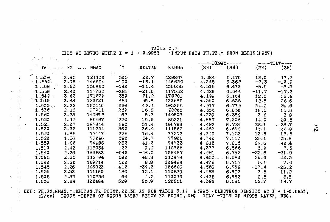
TA:SLE 3.7 'ULT AT LEVEL WHIRE X = 1 + 0.995! -INPUT DATA FH,FZ ,m FROM ELLIS(1957)
; .. ----DX995----- ----TILT----
l'H· .. ·- . FZ , .... ,..,. NMAX m DELTAN NX995 (2H) (3H) (2H) ( 3H)
~~ 1 .53 0 .
2.45 121130 305 22.7 120897 4. 384 6 .576 12.0 1?.7 ·-1.:5e. 2. 'f5 146894 -190 -16.1 146629 4.245 6.368 -7.3 -HJ .9
1 ._e60 .. · 2.63 136890 -140 -11.4 136635 4.315 6.472 -5.5 -8.2 -- 1 .~50 2.40 117763 -285 -21.6 117532 4.429 6.644 -11.7 -17.2
1 .542 . 3.02 171070 350 31.2 170?81 4.1e9 6.164 12.5 18.4 1 :1'510 2.48 122~21 480 35.8 122689 4.350 6.525 18.5 26.6
I 1. e30 ._. 2. 22 103416 620 41:: .1 103205 4. 517 6 .77: 24.2 ~4 .0 .. 1.530 2.16 99011 250 16 .• 8 E8805 4. 553 6 .830 10.5 15.6 1.560 2.78 14987 8 6'7 5.7 149608 4.239 6.359 2.6 3.8
!! 1.520 ~.97 85407 320 19.9 85221 4.667 7 .000 14.0 20 .5 1.52: 2.2? 1 f7014 690 51.4 106799 4.482 6 .724 28.1 38.7 -1.530 2.33 111724 360 26.9 111502 4. 452 6.678 1e.1 22 .0 -.N 1.520 1.85 77447. 275 16.4 772?2 4.749 7 .123 12.5 18.5 1.520 1.86 78096 e90 34.? 77921 4. '7 42 7.113 2::.1 35.0 1.550 1.80 74906 730 41 .0 74733 4.810 7.215 2£.6 40.4 1.510 2.43 118934 122 9. I: 118706 4.3?7 6.566 ::.0 ?.5 1.540 2.26 1e6683 -542 -40.0 106467 4. :01 6. '75 2 -22.6 -31 .9 1 ~545 2.35 113704 600 42.8 113479 4 .453._ - 6.680 22.9 32.3 1.540 2 .3e 1e.9714 120 8.8 109494 4 .478 6. 717 5.1 7.6 1.545 2 .26 1~6823 -412 -3e .3 1066e6 4 .506 6. 75 9 -17.4 -25 .2
. 1.-535 2.32 111100 180 1:!.1. 1108?9 4.462 6.693 7.5 11.2 1.505 2 .32 110236 60 4.~ 110019 4.435 6.653 2.5 3.8 1.5:35 2.44 12 e484 320 23.9 120251 4.394 6.591 12 .7 18.'7
KEY: FH,FZ,NMAX,rn,DELTAN,FZ POINT,2E,3H AS FOR TABLE 3.1; N :>:995 -ELECTRON DENSITY AT X = 1+0 .995Y, el/cc; IX99E -DEPTH OF NX995 LAYER BELOW FZ POINT, KM; TILT -TILT OF NX995 LAYER, DEG.
JI 3
absent during Z echo occurrence.
D) The best Z mode return tilt model proposed by
Papagiannis and Miller has a = 0.24369, b = 0.1. This
corresponds to a minimum tilt (at the bottom of the
ionosphere) of 13.7° and we would thus expect the angle of
incidence of the Z ray to be greater than this (Papagiannis
and Miller do not state what this angle is but our
expectation is verified by ray tracing in Section 3.11).
However, this does not agree with Ellis's observations which 0 0 put the Z echo angle of incidence at 8 to 9 for a dip angle
0 of 72 •
E) Papagiannis and Miller published tne ionograms
shown in Fig.3.44 in support of their proposal. The top
ionogram shows the Z mode occuring over a much wider
frequency range than provided by their "realistic" models.
All the ionograms show spread-F. Lack of spreading on the Z
trace does not imply lack of backscatter because as
Papagiannis and Miller correctly point out .. •••. there is
only one possible path for the z mode echoes ......
Papagiannis and Miller incorrectly state what the condition
of the ionosphere is believed to be in the presence of
spread-F. There have been almost as many spread-F theories
and variants of these theories as there have been research
groups studying this phenomenon. Furthermore, spread-F has
appeared to be different at different locations and at least
snows some form .of latitude dependence. Papagiannis and
Miller have picked a vague form of spread-F which suits the
tilt theory but have provided no evidence to demonstrate
that it is operating for these ionograms. Topside sounding
and intense equatorial studies have brought a degree of
clarification to the spread-F problem and field aligned
structures are currently thought to be responsible for much
more spread-F than "blobby" or ·"wavy" structure. In any
case Ratcliffe and Weekes (1960) did not say that the F
layer assumes a blobby structure during spread-F conditions
but they did say "There is evidence that the spread of the
ecno is caused by scattering in depth rather than by
scattering from irregularities at distances considerably
removed from the vertical reflection point". The presence
of spreading on the iongrams together with lack of spreading
on the Z trace does not yield support for the tilted layer
theory - it merely does not preclude it as it does not
preclude the existence of many other irregularities.
3.11 Ray Tracing
Using the Jones (19?5) ray tracing program, ordinary and
extraordinary type rays were traced in the Papagiannis/Miller
tilt/wedge ionosphere for a = 0.24369 and b = 0.1, with other
parameters as set by Papagiannis and Miller. Papagiannis and
Miller stated that for the Earth's magnetic field they used the
11'5'
standard dipole approximation but did not state what field
strength they assumed on the ground at the equator. However,
from Fig.~.43 it should be possible to determine the gyro
freQuency by calculating the electron densities at the coupling
regions and reflection
frequencies 4.15, 4.225
points. This was done for the
and 4.30 MHz for 9o placed at the
diagram origin but the results were inconsistent with the
requirements of these regions. It was found that wAen 80 was
shifted 39.75 km. equatorward of the diagram origin then self
consistency was achieved for a gyro frequency of 0.867 MHz. on
the ground at the equator. It is not known why B0 is not
coincident with tne diagram origin but it may be an indication
that it is not easy to construct a tilt model naving a
satisfactory frequency spread of returned Z echoes for
reasonable values of a and b. The 0 and X mode frequencies
corresponding to reflection from tne same ionospneric layer as
the Z mode 4.225 MHz ray were then found to be 4.865 and 5.602
MHz respectively. Fig.3.45 shows magnetic meridian ray
tracing, in this ionosphere, of the 4.865 MHz 0 mode for
various zenith angles at 2° intervals and FiR.3.46 is a similar
diagram for the X mode at 5.602 MHz. The 0 mode was also
traced in a similar fashion for 4.225 MHz to find the lower
half of the 4.225 MHz Z mode ray of Fig.3.43 and these traces
are shown in Fig.3.47. The 4.225 MHz 0 mode ray must have a
wave normal angle parallel to the magnetic field direction in
the coupling region in addition to returning to the transmitte~
and this condition was satisfied. To the nearest half degree
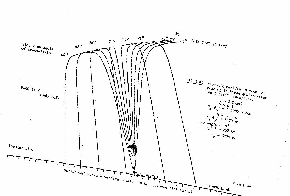
E le vat; on angle of transmission 6
60
FREQUENCY
4. 865 MHz.
Equator side
Horizontal scale ""
82°
~~~ 78° 80° 84° (PENETRATING RAYS)
Vert i ca 1 s c 1 ( 10
a e km. between tick marks)
Magnetic meridian 0 m d tra · • o e ray ''b c1ng in Papagi~nnis-11; I fer
est case'' ionosphere.
a == 0.24369 b == o. 1
Nm(B0 ) == 300000 el/cc
H == 50 km. r ( ~ ) == 662 O km m o ·
Dip an~Te "" 720
zm (0) == 250 km.
R0 "" 6370 km.
Pole side GROUND LEVfL
~
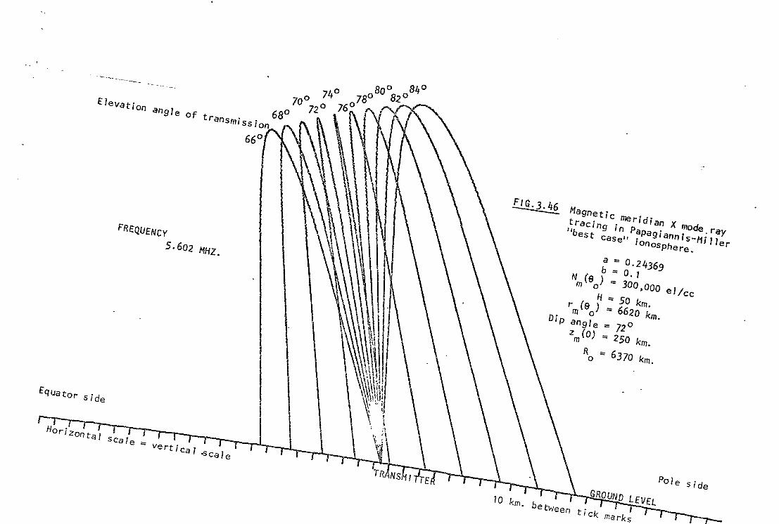
- - - ---- ----- ------- --
tlevatlon angle of transmission
66°
FREQUENCY
S.602 MHZ.
Equator side
Horiz~tol S~le • ••rtica1 ~Cole
~ Hagn~tic meridian X mode.ray tracing in Papagiannis-Hiller ''best case'' ionosphere.
a "' 0.24369 b = o. 1
Nm(e0 ) == 300,000 el/cc
H == 50 km. rm(e0 ) = 6620 km.
Dip angle == 12°
zm (o) == 250 km.
R0 === 6370 km.
GROUND LEVEL I 10 km. between tick marks
Pole Side
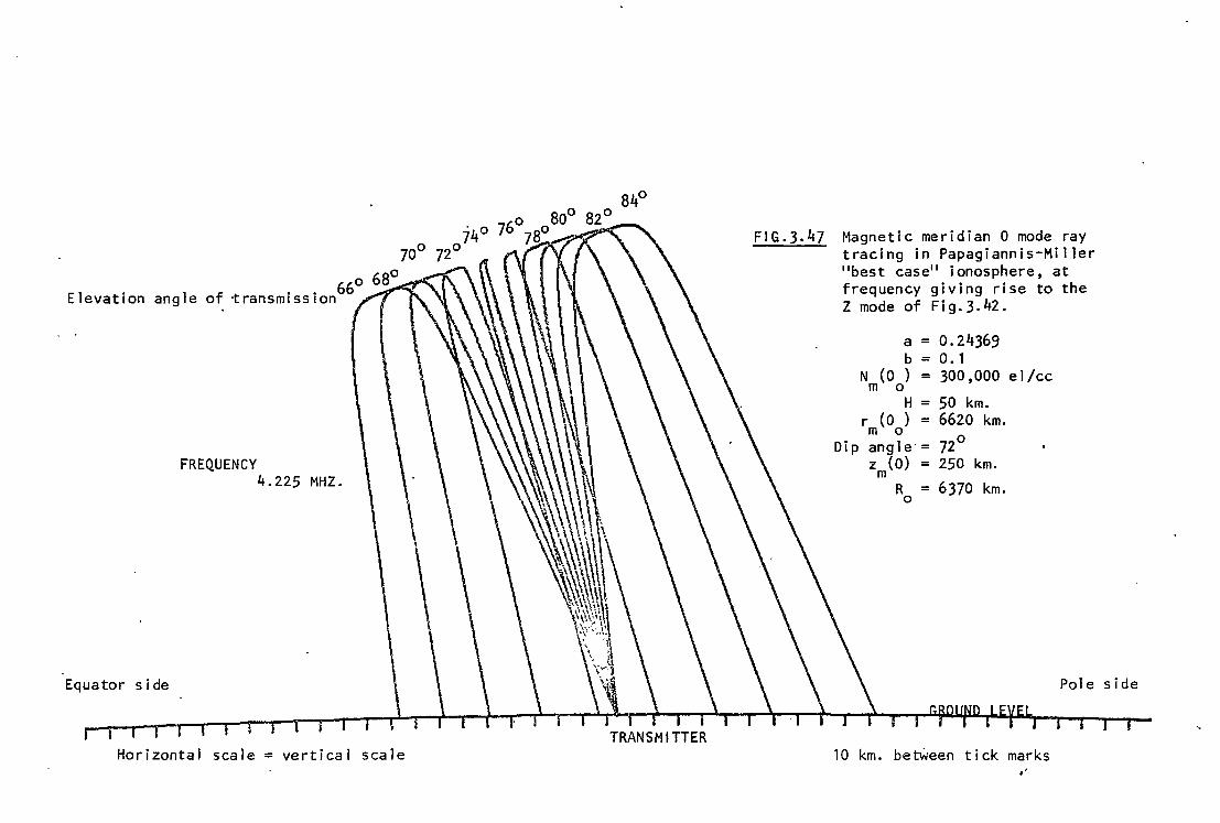
84°
. . 660 680 Elevation angle of transm1ss1on
FREQUENCY 4.225 MHZ.
Equator side
TRANSMIITER Horizontal scale= vertical scale
FIG.3.47 Magnetic meridian 0 mode ray tracing in Papagiannis-Miller 11 best case11 ionosphere, at frequency giving rise to the Z mode of Fig.3.42.
a = 0. 24369 b = 0. 1
N (0 ) m o
= 300,000 el/cc
H = 50 km. r (0 ) = 6620 km. m o
720 Dip angle·= z (0)
m = 250 km.
R 0 = 6370 km.
Pole side
10 km. between tick marks
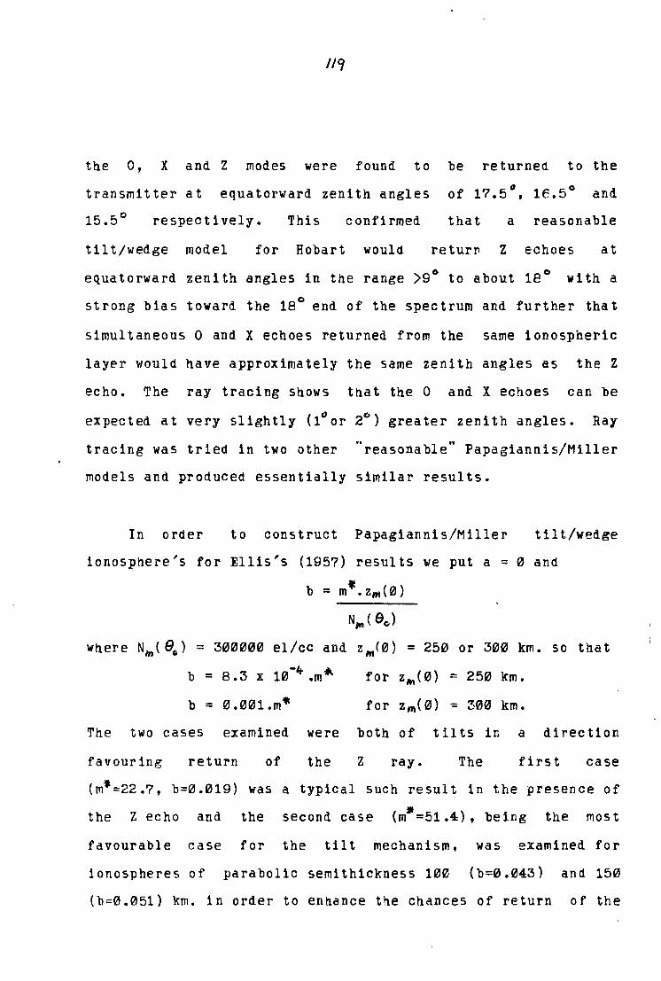
I/Cf
the O, X and Z modes were found to be returned to the
transmitter at equatorward zenith angles 0 0 of 17.5 , 16.5 and
15 .5° respectively. This confirmed that a reasonable
tilt/wedge model for Hobart would retur~ Z echoes at 0 0 equatorward zenith angles in the range )9 to about 18 with a
0 strong bias toward the 18 end of the spectrum and further that
simultaneous 0 and X echoes returned from the same ionospheric
layer would have approximately the same zenith angles as the Z
echo. The ray tracing shows that the 0 and X echoes can be
expected at very slightly (1°or 2°) greater zenith angles. Ray
tracing was tried in two other "reasonable" Papagiannis/Miller
models and produced essentially similar results.
In order to construct Papagiannis/Miller tilt/wedge
ionosphere's for Ellis's (1957) results we put a = 0 and
b = m'.z,,,(0)
N"'(90 )
wnere Nin( eG) = 300000 el/cc and z,,,(0) = 250 or 300 km. so that
b = 8.3 x 10-lt .m*- for zw.(0) = 250 km.
b = 0.001.m'* for Zm(0) ~ 300 km.
The two cases examined were both of tilts i~ a direction
favouring return of the Z ray. The first case
(m'=22.7, b=0.019) was a typical such result in the presence of
the Z echo and the second case (m•=51.4), being the most
favourable case for the tilt mechanism, was examined for
ionospheres of parabolic semithickness 100 (b=0.043) and 150
(b=0.051) km. in order to ennance the chances of return of the
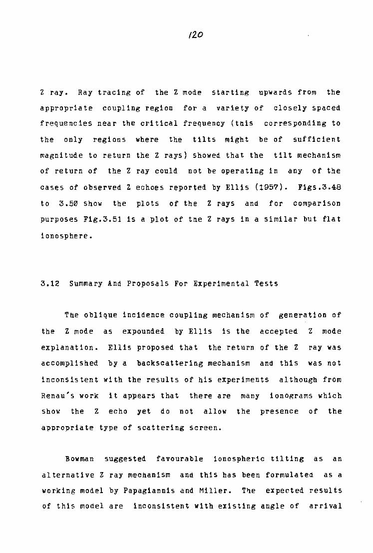
Z ray. Ray tracing of the Z mode starting upwards from the
appropriate coupling region for a variety of closely spaced
frequencies near the critical frequency (tnis corresponding to
the only regions where the tilts might be of sufficient
magnitude to return the Z rays) showed that the tilt mechanism
of return of the Z ray could not be operating in any of the
cases of observed Z echoes reported by Ellis (1957). Figs.3.48
to 3.50 show the plots of the Z rays and for comparison
purposes Fig.3.51 is a plot of tne Z rays in a similar but flat
ionosphere.
3.12 Summary And Proposals For Experimental Tests
The oblique incidence coupling mechanism of generation of
the Z mode as expounded by Ellis is the accepted Z mode
explanation. Ellis proposed that the return of the Z ray was
accomplished by a backscattering mechanism and this was not
although from inconsistent with the results of his experiments
Renau's work it appears that there are many
show the Z echo yet do not allow the
ionograms which
presence of the
appropriate type of scattering screen.
Bowman suggested favourable ionospheric tilting as an
alternative Z ray mechanism and this has been formulated as a
working model by Papagiannis and Miller. The expected results
of this model are inconsistent with existing angle of arrival
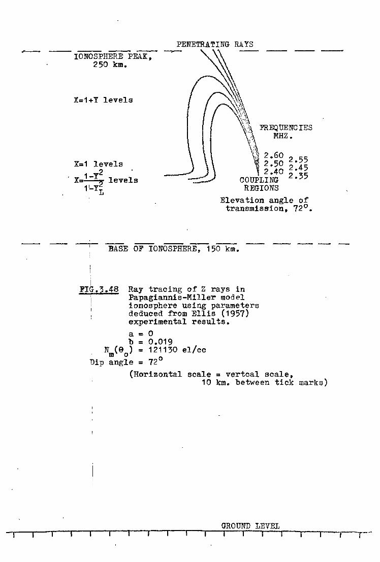
-
- I 1
IONOSPHERE PEAK, 250 km.
X=1+Y levels
X=1 levels 1-Y2 . x-~ levels
1~YL
PENETRATING RAYS
~ ---
~ ~ \'~ \~\
\'.\~ FREQUENCIES :·\ MHZ.
\:9 2 .60 2 55
~ ~:~g 2:45 COUPLING 2 •35
REGIONS Elevation angle of
transmission, 72°.
BASE OF IONOSPHERE, 150 km.
i FIG.3.48 Ray tracing of Z rays in
Papagiannis-Miller model ionosphere using parameters deduced from Ellis (1957)
I
! I
experimental results. a =- 0 b = 0.019
N (0 ) = 121130 el/cc m o 0 Dip angle = 72
(Horizontal scale = vertcal scale, 10 km. between tick marks)
GROUND LEVEL I I
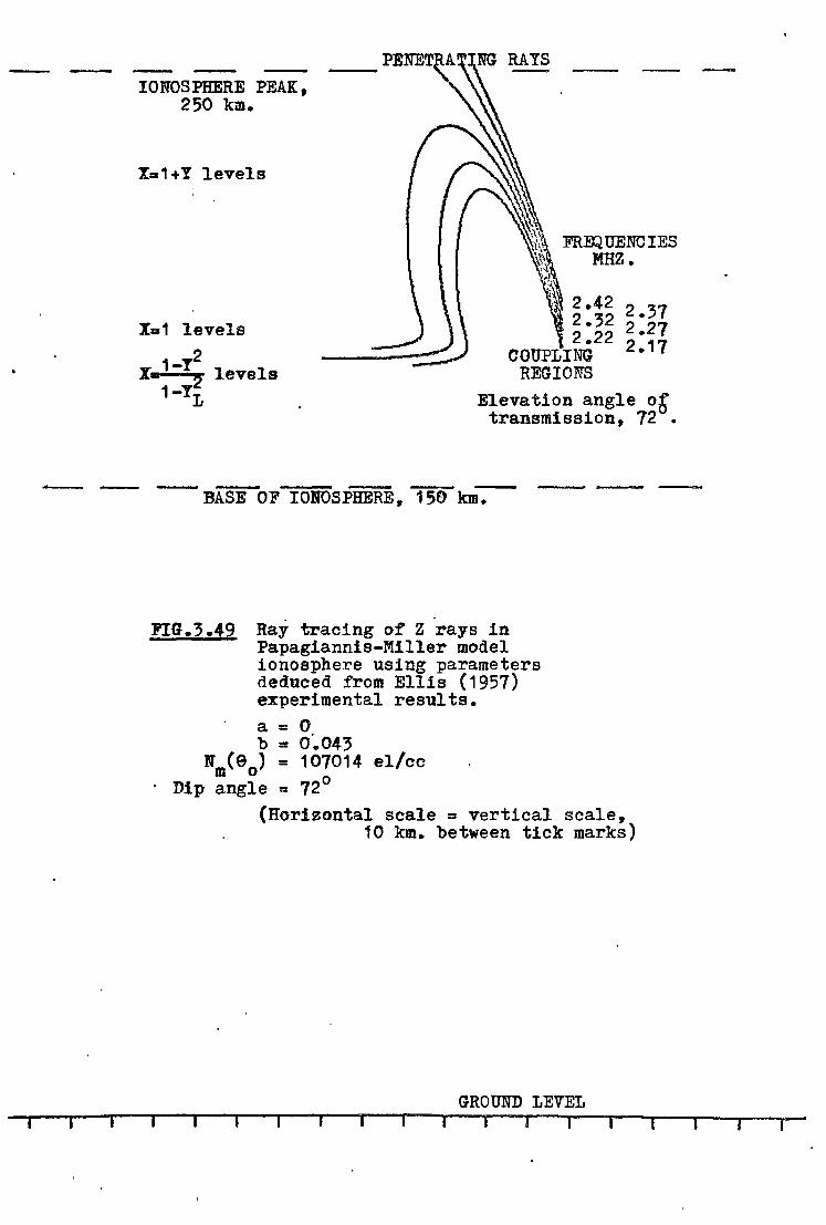
IONOSPHERE PEAK, 250 km.
Xa1+Y levels I .
Xn1 levels 2 x.1-Y levels
FR~UENCIES
1-Yi Elevation angle 06 transmission, 72 •
-- - BASE OF IONOSPHERE, 150 km-=--
FIG.3.49 Ray tracing of Z ·rays in Papagiannis-Miller model ionosphere using parameters deduced from Ellis (1957) experimental results. a= 0 b = o·.043
Nm(00
) = 107014 el/cc Dip angle = 72°
(Horizontal scale = vertical scale, 10 km. between tick marks)
GROUND LEVEL
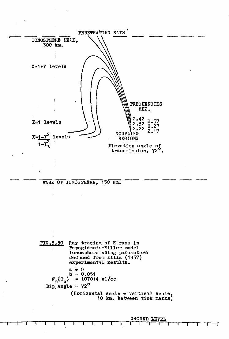
---IONOSPHERE PEAK, 300 km.
X1111+Y levels
X:s1 levels
X•1-Y2 levels 1-Tt .
PENETRATING RAYS
FREQUENCIES MHZ.
2.42 2 37 2.32 2·27 2 22 •
COUPLING 2 • 17
REGIONS Elevation angle o~
transmission, 72 •
BASE OF IONOSPHERE, 150 km. ----
FIG.,.50 Ray tracing of Z rays in Papagiannis-Miller model ionoaphere using parameters deduced from Ellis (1.957) experimental resu1ts. a• 0 b = 0.051
N (e ) • 1.07014 el/cc m o 0 Dip_ angle= 72
(Horizontal scale = vertical scalet 10 km. between tick markSJ
GROUND LEVEL I I I I I I --r-r

IONOSPHERE PEAK' - _PENETRATING RAYS ---2'50 km.
X•1+Y LEVELS
X•1 LEVELS
X=1-Y2 LEVELS 2
FR~UENCIES MHZ.
2.60 2 55 2 .. 50 2·45 2 40 •
COUPLING• 2 • 35 REGIONS
1- TL Elevation angle of transmission, 72°.
BASE OF IONOSPHERE, 150 km.
FIG.3.51 Ray tracing of Z rays 'in a flat ionosphere. (a=O,b=O)
Nm(90
) = 121130 el/cc Dip angle = 72°
(Horizontal scale = vertical scale, 10 km. between tick marks)
--- -
GROUND LEVEL
measurements. There is no satisfactory experimental evidence
in favour of this model.
Papagiannis suggested return of the Z ray by a special
solar zenith angle controlled case of the tilt model. There is
no satisfactory experimental evidence in favour of this model
and existing angle of arrival measurements are all strongly
against it.
Satisfactory physical processes have not been advanced by
the proponents of either the solar zenith angle return
mechanism or the backscatter mechanism. The tilt/wedge return
mechanism operates by means of well accepted physical processes
but its proponents have not explained how the very special
arrangement pf the ionospheric laters is to be generated.
The examination of Papagiannis and Miller's formulation of
the tilt/wedge model shows that the Z echo would have angles of
arrival centred around 14° to 17°N for Hobart with the X and 0
modes from the same ionospheric layer having similar angles of
arrival, the X echo angle of arrival being about a degree
further north and the 0 echo angle of arrival being about two
degrees further north. Simultaneous measurements of the
zenithal angles of arrival coincident witn angles of
transmission of the Z, O and X rays would thus provide two
unambiguous experimental tests of the operation of the
tilt/wedge return mechanism in t~e presence of the Z echo.
J2 {,
Such experiments would also conclusively test the solar zenith
angle return mechanism.
Widening of the returned O and X echo angular spectrum in
the presence of the Z echo would be expected if backscattering
were the operating return mechanism but it is not considered to
be a definitely conclusive test. On the other hand the
complete form of a wide beam h'f ionogram in the presence of
the Z echo can be used to determine the presence or absence of
a scattering screen at the reflection level.
4.1 Introduction
CHAPTER FOUR
OBSERVATIONAL TECHNIQUE
Tbe aim of the observations was to make narrow beam
soundin~s at 1° intervals along tne N-S meridian at fixed and
swept frequency in order to determine the distribution of
angles of arrival of the Z echo and the angular location of the
simultanP.ously occurring X and O echoes. It was also desirable
to make some observations of the Z echo at high repetition rate
in order to obtain information about its temporal behaviour.
From the results it was hoped to be able to decide whether or
not the tilt mechanism was operating.
Wnile narrow beam sounding provides some infor~ation
pertinent to the backscattering mechanism it is felt for
reasons previously outlined that wide beam swept frequency
sounding provides a better test of whether or not the mechanism
is operatin~. Wide beam soundings were provided by a separate
instru~ent.
Hobart is a place of relatively nigh Z echo occurrence.
Bowman used Hobart records to support nis tilt nypotnesis,
Papagiannis used Hobart as the location for his calculations
based on his solar zenith angle moael and Papagiannis and
128
Miller used Hobart values for· the key parameters when
developing tneir most likely tilt configuration. Ellis carried
out his experimental investigation into the Z echo at Hobart
and postulated a backscattering mechanism from his results.
The logical location to carry out further investigations was
therefore Eobart. Hobart's geographic coordinates 0
are 42. e s' 147.3°E and its geomagnetic coordinates are 51.7°5 and 224.3°E.
The declination is 13°E, the dip angle 72° and the total field
at the ground is 0.63· oersted.
Zenith angles equatorward of zenith are assigned a
positive sign and those poleward of zenith a negative sign. As
Hobart is in the southern hemisphere, a positive zenith angle
at Hobart will mean to the north of zenith and a negative
zenith angle to the south of zenith.
4.2 Tbe Instruments
The SOUTH LEA IONOSONDE near Hobart is a Type 4A feeding a
wide beam delta antenna and is operated by the Ionospheric
Prediction Service. Peak power is 5 KW, sweep range 1-22 MHz
in 12 seconds and the maximum repetition rate for h'f ionograms
is every 20 seconds. Under normal operating practices an
1onogram is made every 15 minutes.
The LLANHERNE HF RADIO TELESCOPE situated near Hobart and
12'}
about 18 km. NE of South Lea was used as the antenna of a
narrow beam ionospheric sounding syste~. The antenna was a
square array 609 m x 609 m consisting of 64 east-west rows each
of 32 broadband dipoles. The operating range was 2-18 Mhz, 0 0
~1th corresponding resolutions of 12.4 to 1.4 respectively as
a radiotelescope and 8.8° to 1.0° respectively as an
ionospheric sounder. The beam could be swept through the
meridian in 1° steps from 55° south of zenith to 55° north of
zenith at rates of up to 5° per second. The angular sweep
limits were indvidually adjustable and there was provision for
external control of the beam. Fig.4.1 shows the 5 Mhz profile
of the beam for receiving only at zenith, for sounding at
zenith and for sounding at 5° north of zenith. Fig.4.2 is an
aerial view of the array. The actual steering of the array was
done in terms of integral "beam number" and not in integral
values of declination, the relationship between the beam number
(B) and the zenith angle of the beam (z degrees) being
z = arcsin (B x 0.01745)
However the zenith angles of interest to -this investigation
were not large enough to make the difference between z and B
significant so the zenith angle may be taken as equivalent to
the beam number. Zenith angles north of zenith were defined as
positive and those soutn as negative. The general features of
the array were describ~d in greater detail by Ellis (1972).
At the time of the investigation the array was not in use,
was in inoperable condition and deteriorating at a fast rate.
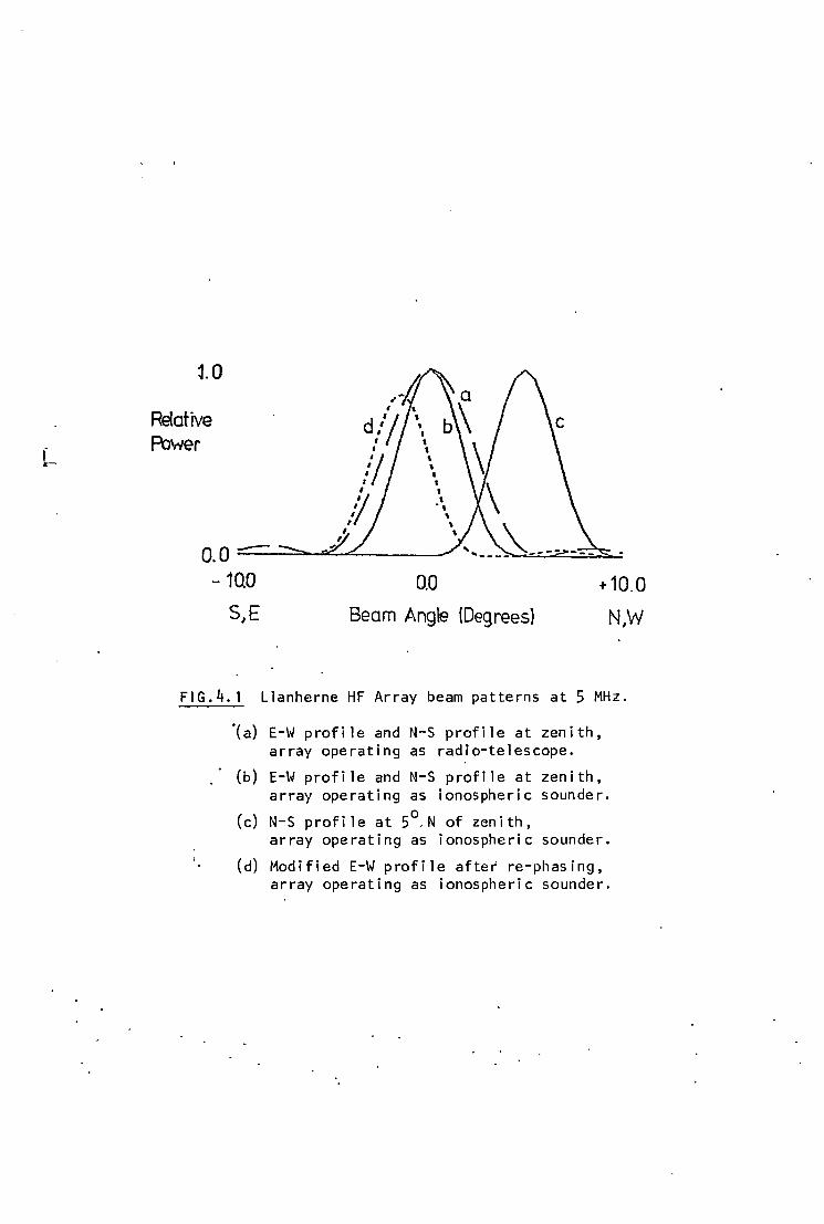
f r-
to
Relative Power
0. 0 ----~-=--==------ 1QO
S,E 0.0
Beam Angle (Degrees)
+10.0
N,W
FIG.4. 1 Llanherne HF Array beam patterns at 5 MHz.
'(a) E-W profile and N-S profile at zenith, array operating as radio-telescope.
(b) E-W profile and N-S profile at zenith, array operating as ionospheric sounder.
(c) N-S profile at 5°,N of zenith, array operating as ionospheric sounder.
(d) Modified E-W profile after re-phasing, array operating as ionospheric sounder.
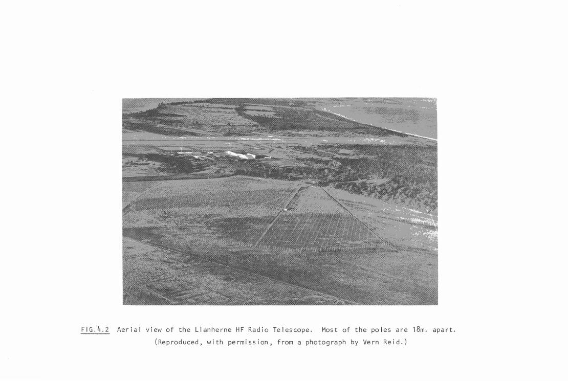
FIG.~.2 Aerial view of the Llanherne HF Radio Telescope. Most of the poles are 18m. apart.
(Reproduced, with permission, from a photograph by Vern Reid.)
Over a period of six months I carried out a massive repair
prograw which brougnt the array into satisfactory operating
condition. I es~imated that it would not be possible to hold
the array in this condition for more than six months. Within
this period the operating system was developed and some
observations made. Consequently it has not been possible to
make further observations following analysis of the data
obtained. Although further observations were desirable the
existing data has nevertheless proved sufficient for the
original purposes.
Each array row of 32 dipoles was connected by a "Christmas
Tree type feed. In order to pnase the array slightly off
zenith in the E-W direction each dipole row was separated into
an east half and a west half (each of 16 dipoles) and the
signal from one half was delayed relative to the other half to
achieve the desired effect. This also had a slight east-west
widening effect on the beam and the resultant modified
east-west profile is shown in Fig.4.1. The transmitted beam
could then be expected to become parallel to the magnetic field
at the 0 reflection level when the beam was pointing about 9°
north of zenith.
The ionosonde used in conjunction with the array was an
IPS Type IIIE modified to produce logarithmic sweep h'f
ionograms from 1.3 to ?.3 Mhz at a rate of four per minute
without loss of resolution or information (fxf2 generally being
133
below ?.5 Mhz at this time). The ionosonde was further
modified to provide two continuously variable receiver gains.
Switching between the two gains could be done either manually
or else automatically at the end of each b'f 1onogram. A
control was also added to allow automatic beam position
increment of one or three degrees at the en~ of each ionogram.
The 10 KW power was reduced to a few watts (about 8 watts,
initially) but as it was found that more power could be fed
into the array tnan had been anticipated the power was
increased to about 200 watts and most of the relevant
observations were made at this power.
In addition to the usual IIIE continuous photographic
record of intensity scan (for production of n'f or h't type
records) a video camera and recorder were set up to record the
A scans displayed on a monitor unit. A second channel on the
monitor unit was set up to offset the position of a marker in
proportion to beam position. The video system recorded at 50
frames per second, the ionosonde pulsed at 50 cycles per second
and the persistence of the CRO monitor unit was such that the
reflection train from each individual pulse could be separatel1
identified. The video tapes lasted about 40 minutes each but
the film ca~acity of the IIIE camera was equivalent to at least
8 hours continuous running. The automatic 3 degree increment
was found to be somewhat unreliable and as video tape could not
be spared for long 3 degree runs, beam position recording was
carried out in these cases bJ attaching a camera to the monitor
134
and displaying only a beam position dot. Such beam position
recording was limited to at most 3 hours duration by the low
film capacity of this camera.
4.3 Observing Programme
As the Z echo is a sporadic phenomenon it was not possible
to institute a programme of unattended recording. The
Llanherne array was visited as often as possible and initially
trial film recording was carried out followed by trial film and
video recording. These early records were made in September
and October of 19?? (Video records from mid-October). Few Z
echoes were seen on the films and none on the video tapes which
were wiped for re-recording. By early November it had become
possible to identify the presence of Z echoes by observing the
echoes on the various monitor units and so Llanherne was visted
more often but recording was commenced only if Z echoes were
identified as present. As South Lea is much closer to the
Physics Department than is Llanherne, the South Lea monitor was
also frequently checked but it was found that the half hour
travel time from South Lea to Llanherne was often sufficient
for the disappearance of the Z echo before recording could take
place.
The main Z echo results were obtained during November
1977. The film recording and video recoraing were normally
13/)'
carried out simultaneously though in many cases film recording
continued well after the video tapes were finished. Records
of h'f type were produced every 15 seconds and at the end of
each frame the beam position incremented by 1° and the gain
changed to the alternate setting. The beam scan limits vere
normally set at 10° S and 21° N ,the bias towards north angles
being because all theories predicted the Z echo to occur in the
approximate 0 range 9 N to 18°N. The two gains were Sl!t by
experience, one high to allow the Z echo to be detected and the
other low to avoid the saturated O and X echoes normally
obtained at high gain levels. Beam change limits of 4° N and
14° N, 20° Sand 20 °N, 25° Sand 25° N were used on occasions.
Some fixed frequency records were also made with the beam
scanning at 5° per second with manual gain chanRes. The scan
limits for this type of recording were 10°S and 21°N, 20°S and
20°N, 21°S and 21°N, 25°S and 25°N. The Z echoes were observed
at various times of the day and night.
4.4 Analysis
Films displaying Z echoes were scaled to provide angle of
arrival information and the 0 and X h'f traces were examined
for variation with angle which might indicate the presence of a
scattering screen. Wide beam ionograms from South Lea for the
same observing period were also examined for evidence of
scattering screens. The video records were analysed to provide
echo strength information at various angles and frequencies.
On the low gain records the noise was generally insignificant
com~ared with the O and X echoes but on the hign gain records
the noise was sufficiently strong compared with the Z echoes
for it to be worthwhile making an estimate of the noise
contribution. This was done by measuring the noise peaks wnich
occurred at about 50 km. greater virtual height than the Z
echo. This provides a reasonable estimate assuming that the
noise occurs independently of the transmitted pulses.
During fast scans tne beam stayed at a particular angle
for about 10 pulses. Examination of the video records showed
that the first one or two records of a particular beam position
displayed interference from the automatic process of re-phasing
the array to reposition the beam. These records were discarded
from the analysis. The remaining 8 or 9 recorQS were scaled
for either Z echo strength or else 0 and X echo strength as
appropriate. The values were squared to obtain relative power
and then averaged to provide a single power value for the
particular mode at each beam position. In the case of tne Z
mode the estimated effect of the noise was removed from the
result. In order to maintain uniformity the measurements were
expressed as a fraction of the voltage of the virtual heignt
rnark~rs. Comparison of the Z echo strength with that of the X
and 0 modes was possible through knowledge of the gains used
when recording. Analysing tne video tapes for amplitude
information was found to be extremely time consuming •. The time

137
taken to analyse the data was generally well over tnree hundred
times as long as the time taken to record it. Since the same
information was usually recorded on film there existed the
possibility of obtaining reasonably accurate amplitude
information by determining the density variations of the film.
T~e problems encountered with this sort of information
retrieval are the non-linear nature of the photographic
processes and the limited density range of the film.
Investigation of the process and some calibration tests using
the original equipment assisted in assessing t~e viability of
the method but the most conclusive test of its validity was
provided by comparing amplitude results made by the film reader
with those measured from the video records (Fig.4.3).
A film density reader was constructed and consisted mainly
of a phototransistor mounted on the x-travelling bar of an x-y
plotter. An image of the film was projected downwarns onto the
bed of the plotter and a ramp generator fed into the x
terminals moved the bar mounted detector smoothly across the
region of interest. Since the recording pen was also mounted
to tne bar (and travelled backwards and forwards along it as
the output from the detector varied) the x component of the
plot was automatically scaled no matter how irregular the x
motion might be. The direction of traverse was invariably in
the direction of the film's time axis. On the b'f records the
virtual height of the Z echo was determined and
X and O ~ode echoes at this virtual height
traversing the
for each angle
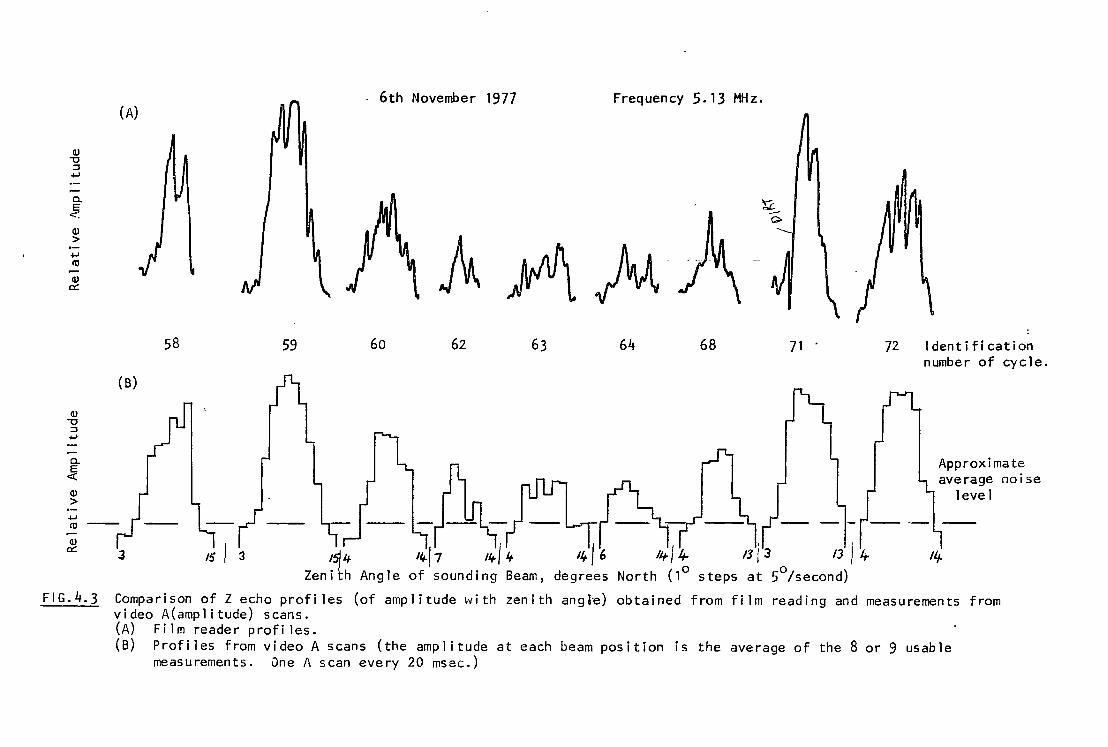
Q) "'C
::::J .µ
c. E < Q)
> .µ
ro Q) c::
Q) "'C
::::J ....,
c. E <(
Q)
> .µ cu Q) c::
FIG.4.3
(A)
58 59
( B)
3 is I 3
- 6th November 1977 Frequency 5 . 1 3 MHz.
60 62 64 68 71 . 72 Identification number of cycle.
-----MA- --1- --Approximate ave rage noise
level
,~ 4 14-/ 7 11,. / it- 14 / 6 It;. / ~ 13 i 3 13 I 4 '"-Zenith Angle of sounding Beam, degrees North (1 steps at 5°/second)
Comparison of Z echo profiles (of amplitude with zenith angle) obtained from film reading and measurements from video A(amplitude) scans. (A) Fi Im reader profi Jes. (B) Profiles from video A scans (the amplitude at each beam position is the average of the 8 or 9 usable
measurements. One A scan every 20 msac.)
provided the variation in echo strength with angle for these
modes. Choosing the same virtual height for the modes is
effectively choosing the same height region in the ionosphere
(for this region of interest) and in the case of the modes also
having the same angle of arrival we are looking at echoes from
the same part of the ionosphere (see sections 3.11 and 3.12).
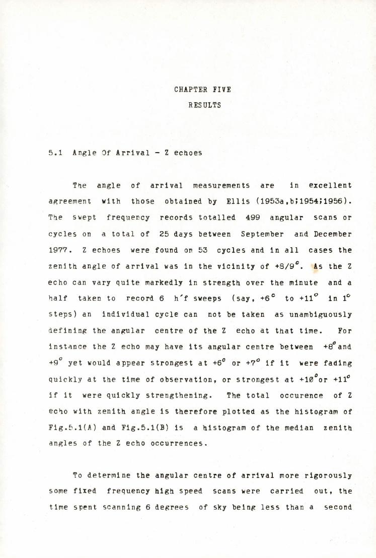
CHAPTER FIVE
RESULTS
5.1 Angle Of Arrival - Z echoes
The angle of arrival measurements are in excellent
aRreement with those obtained by Ellis (1953a,b;1954;1956).
The swept frequency records totalled 499 angular scans or
cycles on a total of 25 days between September and December
197?. Z echoes were found on 53 cycles and in all cases the
zenith angle of arrival was in the vicinity of +8/9°. As the Z
echo can vary quite markedly in strength over the minute and a
~alf taken to record 6 h'f sweeps (say, +6° to +11° in 1°
steps) an individual cycle can not be taken as unambiguously
defining the angular centre of the Z echo at that time. For
instnnce the Z echo may have its angular centre between 0 +8 and
+9° yet would appear strongest at +6° or +7° if it were fading
quickly at the time of observation, or strongest at +10°or +11°
if it were quickly strengthening. The total occurence of Z
ec~o with zenith angle is therefore plotted as the histogram of
Fig. 5 .l(A) and Fig.5.l(B) is a histogram of the median zenith
angles of the Z echo occurrences.
To determine the angular centre of arrival more rigorously
some fixed frequency high speed scans were carried out, tne
time spent scanning 6 degrees of sky being less than a second
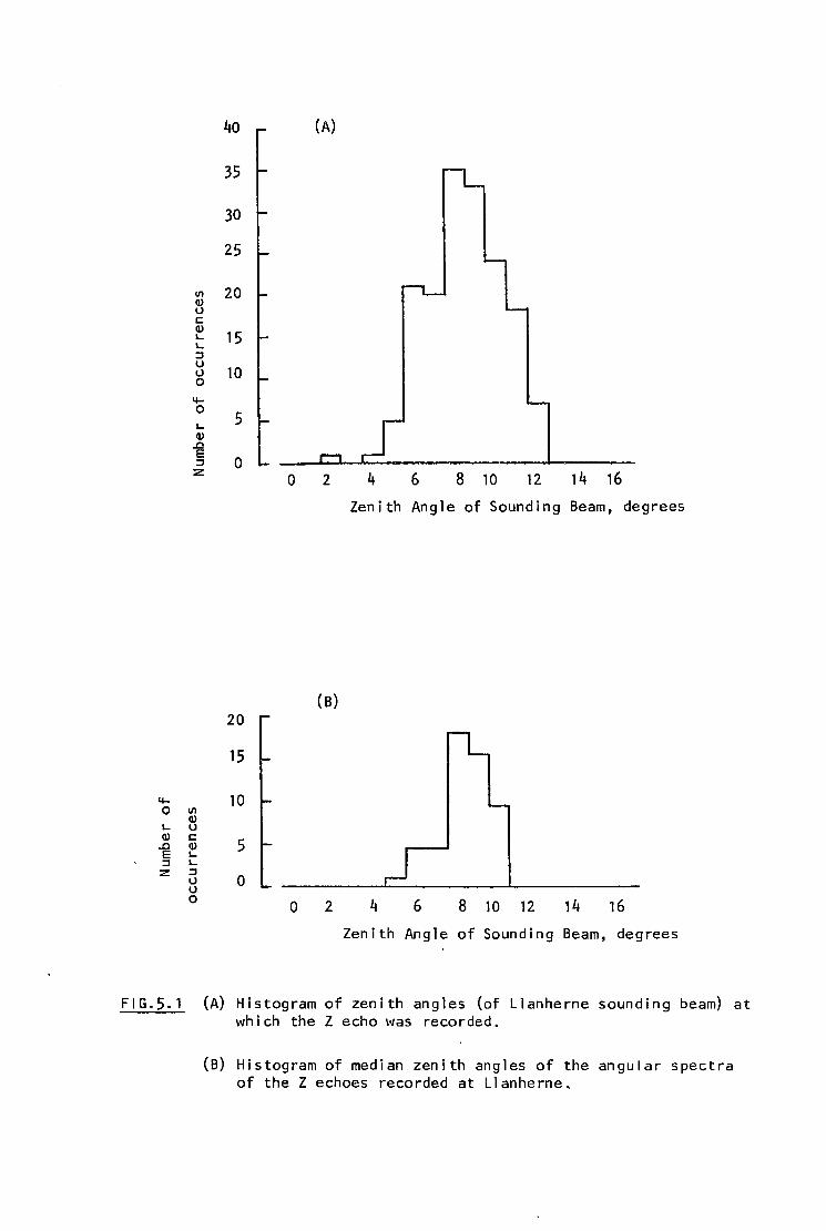
40 (A)
35
30
25
l/I 20 Q) u c: Q)
15 L.. L.. :I u
10 u 0
4-0
5 L.. Q)
..0 E
0 :I z
0 2 4 6 8 10 12 14 16
Zeni th Angle of Sounding Beam, degrees
( B) 20
15
4- 10 0 l/I
Q) L.. u Q) c:
5 ..0 Q) E L.. :I L.. z :I
0 u u 0 0 2 4 6 8 10 12 14 16
Zenith Angle of Sounding Beam, degrees
FIG.5.1 (A) Histogram of zenith angles (of Llanherne sounding beam) at which the Z echo was recorded.
(B) Histogram of median zenith angles of the angular spectra of the Z echoes recorded at Llanherne.
and a half. Examples of the records obtained are s~own in
Figs.5.2 to 5.4, 5.31 to 5.33 and 4.3. It can clearly be seen 0
from tne examples that the Z echo returns cluster around +8/9
and this is also true of those examples not shown here.
On no records were Z echoes found centred around angles
intermediate between 0 0
+11 and +18 • 0
seen in the vicinity of +18 •
5.2 Angle Of !rrival - 0 And X Echoes
No Z echo returns were
Figs.5.5 to 5.11 are typical examples of the angular
variation of the O and X echo strengths at the Z mode virtual
height in the presence of Z echoes. It can be seen that the
angular centre of the 0 and X echoes is sometimes negative,
sometimes positive but in only one case was it found to be
around +9°; that is, in the same direction as the Z echo
(Fig.5.12). The returned 0 and X beams were variable in width
during the presence of the Z echo but showed much the same sort
of variation during its absence. The angle of arrival of the
centre of the O and X beams appeared to be similarly unaffected
by the presence or absence of the Z echo. A relatively common
feature of the O and X echo distributions on cycles detecting Z
echoes, and often on cycles not detecting Z echoes but adjacent
to those displayin~ the Z trace, was a strengthening of the 0
and X echoes in tbe general angular region of the Z echo,
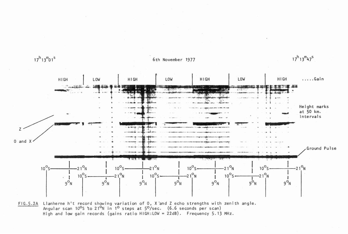
HIGH LOW
-
10°5 21°N I I 10°5
9°N
- 1· - - -------·
10°5 I I
I 21°N I
6th November 1977
LOW
• t
HIGH
-·· -- - ...... -.........--.-.. -- .... _ . '
=· ' -., -·-''"'"·.---.--------- __________ __.
; ~ --- .
__ __,._... ..........,._ __ .
21°N 10°5 21°N I
10°5 I 21°N I 10°5
9°N 9°N 9°N 9°N
LOW HIGH ..... Gain
. _..,. . ..... - . . . ~ --·
- -- --
I 9°N
• I
Cl . i
- 1
. . .
a
.
Height marks at 50 km. intervals
10°5 -----21°N I I
9°N
21°N
FIG.5.2A Llanherne h 1 t record showing variation of 0, X 'and Z echo strengths with zenith angle. Angular scan 10°5 'to 21°N in 1° steps at 5°/sec. (6.6 seconds per scan) High and low gain records (gains ratio HIGH:LOW = 22dB). Frequency 5. 13 MHz.
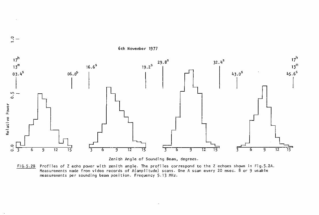
1.. Q)
3: 0
a.. Q)
> .µ re Q)
c::
0
6th November 1977
17h
13m 16.6s 29.as 32.4s
19.2s
03. 4s 06. OS· 43.os
I I I Lt'\-
0
0 . 0 9 12 15 9 12 9 3 9
Zenith Angle of Sounding Beam, degrees.
FIG.5.28 Profiles of Z echo power with zenith angle. The profiles correspond to the Z echoes shown in Fig.5.2A. Measurements made from video records of A(amplitude) scans. One A scan every 20 msec. 8 or 9 usable measurements per sounding beam position. Frequency 5. 13 MHz.
17h
13m
45.6s
I
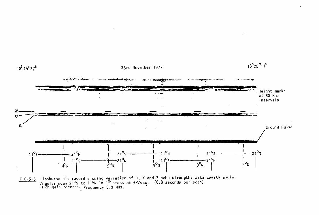
23rd November 1977
a ...
*'~ Height marks at 50 km. intervals
z--- -o--~:;;.;::::.:11 .. 11:111:===:::==-..:::::i•1:111:1 ...... ==;;:::~-==== ... ~1·1:m ...... 1m;=--::;-::::::11m1:: ........ :::.:::::::.=..;:c ...... .:=,~·-~= -~ Ground Pulse
----~ ...... --...... -....--........ --------/ I ] I ------
1--2 1°N l I 9°N
21°5 21°N I 21°5 J 21°N 21°5
2115 t_--21°t~ I 21°5 2 lrH 9°N 9° N 90N I 90N I FIG.5.3 Llanherne h 1 t record showing variation of 0, X and Z echo strengths with zenith angle.
Angular scan 21°5 to 21°N in 1<>- steps at 5°/sec. (8.8 seconds per scan) High gain records. Frequency 5.9 MHz. '
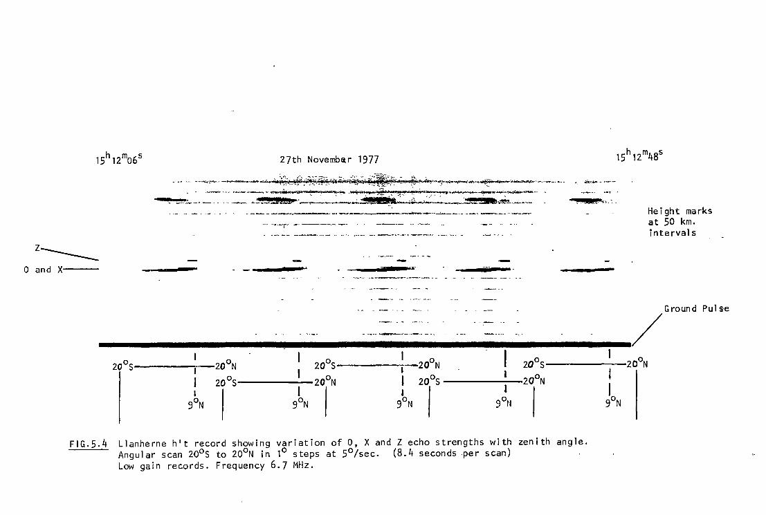
27th Novemba.r 1977
- """ ~- -~~--~~ ... ~r'?D ~.~:~i~1£i~~!~f:·[email protected]~1~fi~!~7"1 ~~-~--~~:..~·=--·L".__.,,. ••
.. .., .. .-.-:.- ... ~-' .... .-. .. -..-.-., ..... ~~ • ;~ 1, 1 -~*~,_7Jse!~ .. ·-~ ;'; *::".- ,--:-u-·~~..-.0....=7~·- ,.. _ .... - .• ~-- .. -· .... -·- 4 ____ £3§Zlw · ------~--~-.!!:lllh~-----------.• _ .. ___ .. ...._ _______ , --·----- ... -------
-- ----- --- ---~--- -- - - --.. - ..... ---'
z------0 and X---
--·~-
Height marks at 50 km. intervals
Ground Pulse
-----------··------------_.. ______ / 20°s~---~:,~20°N 20°s~-----!--20°N 20°s~---~-1 ---20°N
I 20°s-----1
-20°N l 20°s -----1-20°N I
l I I I I 9°N 9°N 9°N 9°N 9°N
FIG.5.4 Llanherne h't record showing variation of 0, X and Z echo strengths with zenith angle. Angular scan 20°s to 20°N in 1° steps at 5°/sec. (8.4 seconds .per scan) Low gain records. Frequency 6.7 MHz.
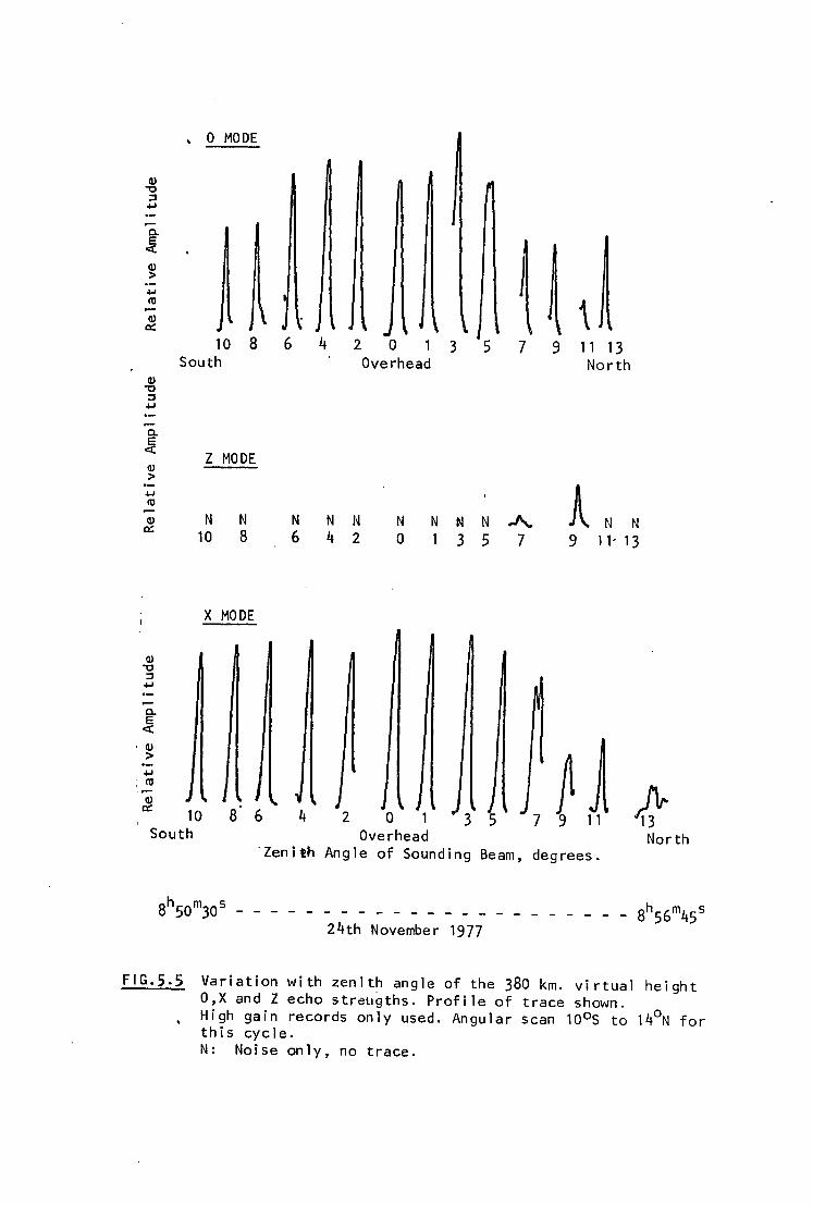
' 0 MODE
Q) -0 ::I +"
a. E
<(
Q) > +"
\ Ill
Q) ~
10 a 6 4 2 0 3 5 7 9 11 13 South Overhead North
Q) -0 ::I +"
a. E
c:( Z MODE
Q) >
A +" Ill
Q) N N N N N N N N N A N N ~ 10 a 6 4 2 0 1 3 5 7 9 11· 1 3
X MODE
Q) -0 ::I +"
a. E
c:(
ft 1 ' Q) > +"
: Ill
Q) ~ 10 a 6 4 2 0 3 5 7 9 11 f( South Overhead North
·zenith Angle of Sounding Beam, degrees.
ah m s 50 30 - - - - -24th November 1977
ah 6m s - - - - - - - - 5 45
FIG.5.5 Variation with zenith angle of the 3ao km. virtual height O,X and Z echo strc11gths. Profile of trace shown. High gain records only used. Angular scan 10°s to 14°N for this cycle. N: Noise only, no trace.
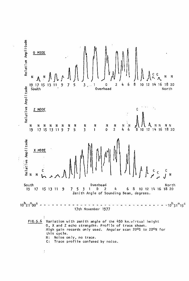
Q) "'C :I .....
0. 0 MODE
~J e ct Q)
> .....
fiRt A~ Ill
A Q)
)\ C C N a:: N A _N N
I\ .I\.
19 17 15 13 11 9 7 5 -3 ' -. 0 2 4 6 8 10 12 14 16 18 20 Q) sou.th Overhead North "'C :I .....
0. e ct Q)
Z MODE c > .....
~A~ N
Ill
Q) I a::
N N N N N N N N N N N N N '.N N N N 19 17 15 13 11 9 7 5 3 1 0 2 4 6 8 10 12 14 16 18 20
Q) -0 :::J .µ
X- M&D£ 0. e ct
• Q)
~fil\~ .> • .µ . Ill c
Q)
N N a:: ~
South Overhead North 19 17 15 13 11 9 7 5 3 1 0 2 4 6 8 10 12 14 16 18 20
Zenith Angle of Sounding Beam, degrees.
h m s 10 21 00 - - - - - - - - h m s - - - - - - - - - - - - - -10 31 15 17th November 1977
FIG.5.6 Variation with zenith angle of the 450 km.virtual height 0, X and Z echo strengths. Profile of trace shown. High gain records only used. Angular scan 20°s to 20°N for this cycle. N: Noise only, no trace. C: Trace profile confused by noise.
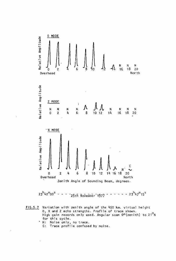
Q) 0 MODE
" ::J ,j..I
a.. E
J <x: Q)
> ,j..I
ra Q.l c:: 0 2 Overhead
Q.l
" ::J ,j..I
a.. Jf Q)
> ,j..I
ra Q) c::
Q.l
" ::J ,j..I
a.. Jf Q.l
> ,j..I
ra Q.l c::
Z HOOE
N N 0 2
--x MO-OE
0 Overhead
N 4
2 4
Zenith
6
N1 6·
6
Angle
~ 1 .{\ N N N 0 1_6_ 18 20
North
f\. )A N N N N 8 10 12 14 16 18 20
J A A fi c N' ~
8 10 12 14 16 18 20 North
of Sounding Beam, degrees.
23h
42m
00s _ _ _ h
4 m s
-25th November-1977 - - - - - - 23 7 15
FIG.5.7 Variation with zenith angle of the 450 km. virtual height 0, X and Z echo strengths. Profile of trace shown. High gain records only used. Angular scan o0 (zenith) to 21°N for th i s eye 1 e.
• N: Noise only, no trace. C: Trace profile confused by noise.
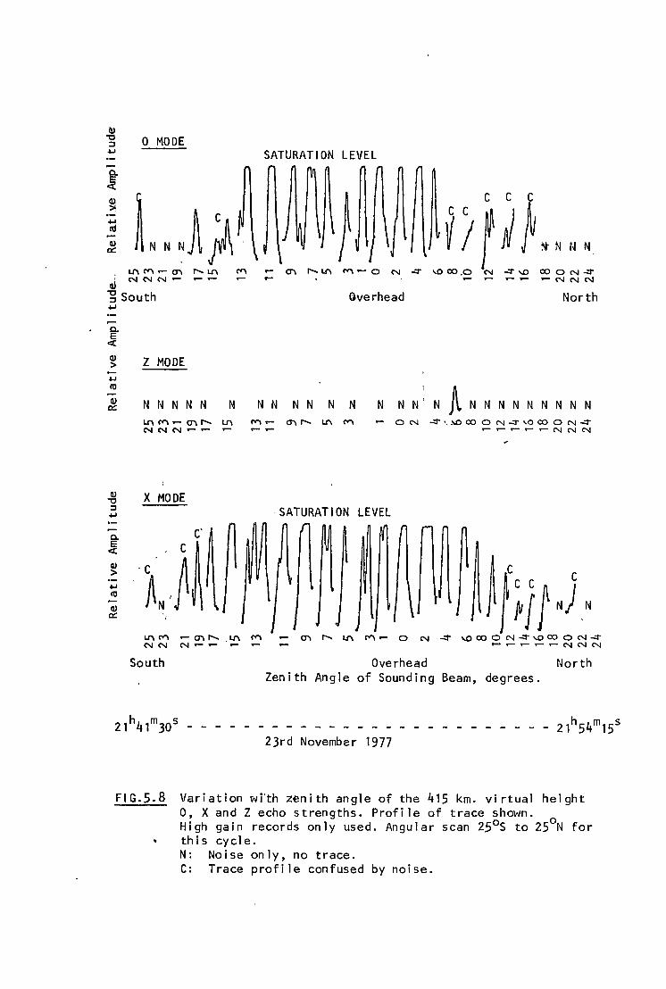
0 MODE SATURATION LEVEL
} Lt'\ M .- en ai NNN.-
r-.. Lt'\ ........ -g South Overhead North .....
0.. E <(
Q)
>
Q) "'O
:::J .....
a. ~ Q) > ..... rtl
Q) 0:::
Z MODE
N N N N N N N N N N N N N N N ' N ~ N N N N N N N N N Lt'\ M ..... en r-.. Lt'\ M ..... en r-.. Lt'\ M N N N ...- .-
0 N ~ '-~ CO 0 N ~ 'O CO 0 N ~ .....- ,...- ,-- r- ,.... N N N
X MODE
South
-SATURATION LEVEL
en r-.. Lt'\ M.- 0 N ~ \.OCOON~\.OCOON~ .-.--.....-...--NNN
Overhead North Zenith Angle of Sounding Beam, degrees.
h m s 21 41 30 - - - - - h 1.m s - - - - - - - - - - - 21 5~ 15 23rd November 1977
FIG.5.8 Variation wi'th zenith angle of the 415 km. virtual height 0, X and Z echo strengths. Profile of trace shown. High gain records only used. Angular scan 25°s to 25°N for this cycle. N: Noise only, no trace. C: Trace profile confused by noise.
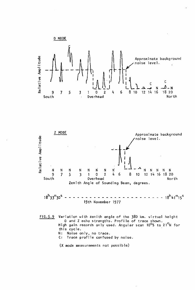
Q)
" ::J .µ
c. E <(
Q)
> .µ
"' Q) a::
Cl. E <(
Q)
> .µ
"' Q) a::
0 MODE
~ t--~ 9 7
South
Z MODE
N N 9 7
South
5
N 5
3
N 3
'f I I
I fl I I 1 ___ I
0 2 Overhead
N 1
N 0
Overhead
N 2
Approximate background /noise level .
\i_L)_ ~_; c N J_N
4 6 8 10 12 14 16 18 20 North
Approximate background
' N. !._1_ . .11.N N N N N
4 6 8 10 12 14 16 18 20 North
Zenith Angle of Sounding Beam, degrees.
ah m s 1 33 30 - - - -
h m s - - - - - - - - - - - - - - - - - 18 41 15 19th November 1977
FIG.5.9 Variation with zenith angle of the 380 km. virtual height 0 and Z echo strengths. Profile of trace shown.
High gain records only used. Angular scan 10°s to 21°N for this cycle. N: Noise only, no trace. C: Trace profile confused by noise.
(X mode measurements not possible)
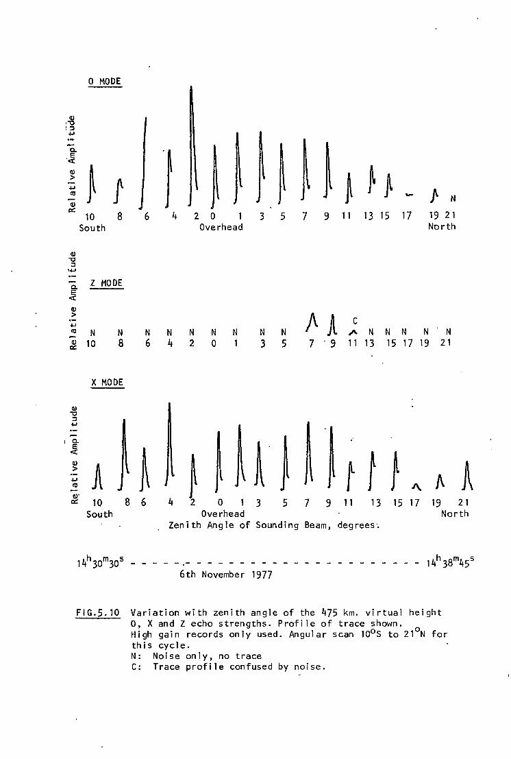
0 MODE
Q) •'"O : :I
""' a.
i E
•ct:
Q)
~ ~ ~ i >
f ""' f ltJ "'" Ii Q)
CIC 8 6 10 4 2 0 3 5 7 9 l l 13 15 17 19 21
South Overhead North
Q) '"O ::J
'""' a. Z MODE E
<(
Q)
> /\A ""' c
ltJ N N N N N N N N N """
N N N N . N Q) 10 8 6 4 2 0 1 3 5 7 . 9 11 13 15 17 19 2 1
CIC
X MODE
Q) '"O ::J
""' I 0.
A} .
E
~ ct:
~ f } Q)
A t A > l ""' /\ ltJ I\ Q)"
8 6 4 CIC 10 2 0 3 5 7 9 11 13 15 17 19 21 South Overhead North
Zenith Angle of Sounding Beam, degrees·.
4h m s 1 30 30 - - - -h m s - - - - - - - - - - - - - 14 38 45
6th November 1977
FIG.5. 10 Variation with zenith angle of the 475 km. virtual height 0, X and Z echo strengths. Profile of trace shown. High gain records only used. Angular scan l0°s to 21°N for this cycle. N: Noise only, no trace C: Trace profile confused by noise.
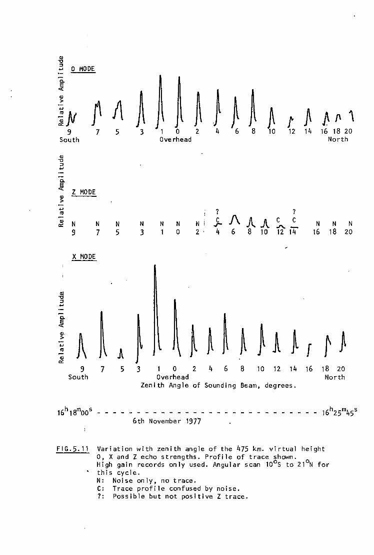
Cl,) -0 :::J 0 MODE ... a. E
<C
Cl,)
~ } ~ ~ ~ > p /\ +.J
~ } ~JV f }.. /\ '\ 9 7 5
South
Cl,) -0
:::J +.J
a. ~ Z MODE Cl,)
> +.J I'll
Cl,) N N N a:: 9 7 5
X MODE
cu -0 :::J +.J
a. ~ Cl,).
A > +.J I'll .A Cl,)
a:: 9 7 5
South
3 0 2 4 8 10 12 14 16 18 20 Overhead North
7 ?
N N N N c f\ .A .A c c N N N ..r- .,,...,. -3 1 0 2 4 6
~ ~ ~ 3 0 2 4 6
Overhead Zeni th Angle of Sounding
6th November 1977
8 10 12 14 16 18 20
A }A ~ f t ~ 8 10 12 14 16 18 20
North Beam, degrees .
6h m s - - - - - - - - - - 1 25 45
FIG.5. 11 Variation with zenith angle of the 475 km. virtual height 0, X and Z echo strengths. Profile of trace shown. High gain records only used. Angular scan 10°s to 21°N for this cycle. N: Noise only, no trace. C: Trace profile confused by noise. 7: Possible but not positive Z trace.
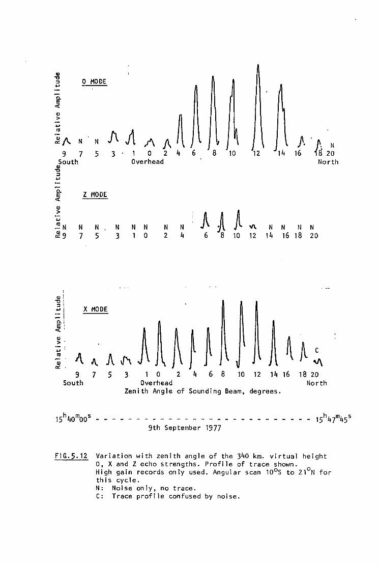
Q) ,, 0 MODE :J .....
a. E
c::t Q)
~ > ..... l1J
f\ A :;;_ f\.. N N /\ A f .. . N 16 fa 9 7 5 3 . 0 2 4 6 8 10 12 14 20
South Overhead North Q) ,, :J .....
-a. Z MODE E c::t Q)
A >
A A ..... ~N N N N N N N N 'II\ N N tJ N ~9 7 5 3 1 0 2 4 6 8 10 12 14 16 18 20
I
Q) I
~I x MODE
~I c::t I
Q)
>' ..... l1J
Q)
a: ' 9
South
/\. A 7 5
~ ~~} ~A c
'"' '\/\ 3 0 2 4 6· 8 10 12 14 16 18 20
Overhead North Zeni th Ang 1 e of Sounding Beam, degrees.
h4 m s 15 0 00 - - - - - - h m4 s - - - - - - - - - - - 15 47 5 9th September 1977
FIG.5.12 Variation with zenith angle of the 340 km. virtual height 0, X and Z echo strengths. Profile of trace shown. High gain-records only used. Angular scan 10°s to 21°N for this cycle. N: Noise only, no trace. C: Trace profile confused by noise.
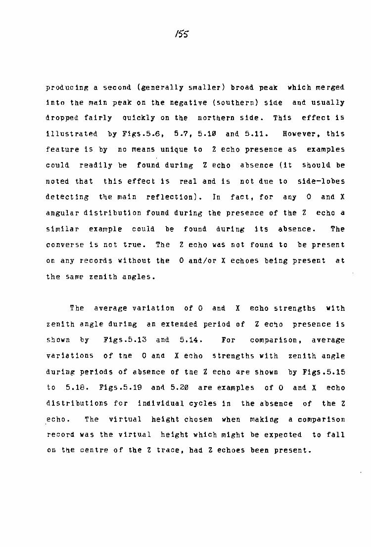
fS5
producing a second (generally smaller) broad peak which merged
into the main peak on the negative (southern) side and usually
dropped fairly Quickly on the northern side. This effect is
illustrated by Figs.5.6, 5.7, 5.10 and 5.11. However, this
feature is by no means unique to Z echo presence as examples
could readily be found during Z echo absence (it should be
noted that this effect is real and is not due to side-lobes
detecting the main reflection). In fact, for any 0 and X
angular distribution found during the presence of the Z echo a
similar example could be found during its absence. The
converse is not true. The Z echo was not found to be present
on any records without the O and/or X echoes being present at
the same zenith angles.
The average variation of 0 and X echo strengths with
zenith angle during an extended period of Z ec~o presence is
shown by Figs.5.13 and 5.14. For comparison, average
variations of t~e 0 and X echo strengths with zenith angle
during periods of absence of tne Z echo are shown by Figs.5.15
to 5.18. Figs.5.19 ann 5.20 are examples of O and X echo
distributions for individual cycles in the absence of the Z
echo. The virtual height chosen when making a comparison
record was the virtual height which might be expected to fall
on tne centre of the Z trace, had Z echoes been present.
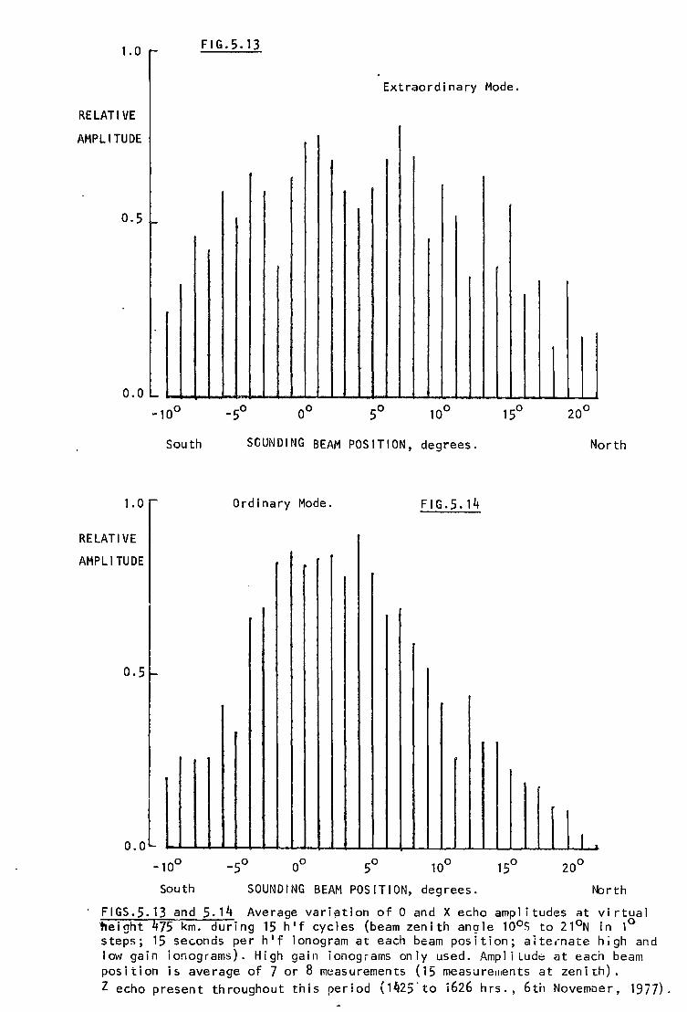
1. 0
RELATIVE
AMPLITUDE
0.5
o.o
1. 0
RELATIVE
AMPLITUDE
0.5
0.0
-100
South
-100
South
FIG.5.13
Extraordinary Mode.
-50 00
SOUNDING BEAM POSITION, degrees. North
Ordinary Mode. FIG.5.14
I . -5° o0 5° 10° 15°
SOUNDING BEAM POSITION, degrees. thrth
FIGS.5. 13 and 5. 14 Average vari~tion of 0 and X echo amplitudes ~t virtual ~eight 475 km. during 15 h'f cycles (beam zenith angle 10°s to 21°N in 1° steps; 15 seconds per h 1 f ionogram at each beam position; alternate high and low gain ionograms). High gain ionograms only used. ,l\mpl i Ludt: at each beam position i5 average of 7 or 8 measurements (15 measure111ents at zenith). Z echo present throughout this period (1425.to 1626 hrs., 6th Novemoer, 1977).
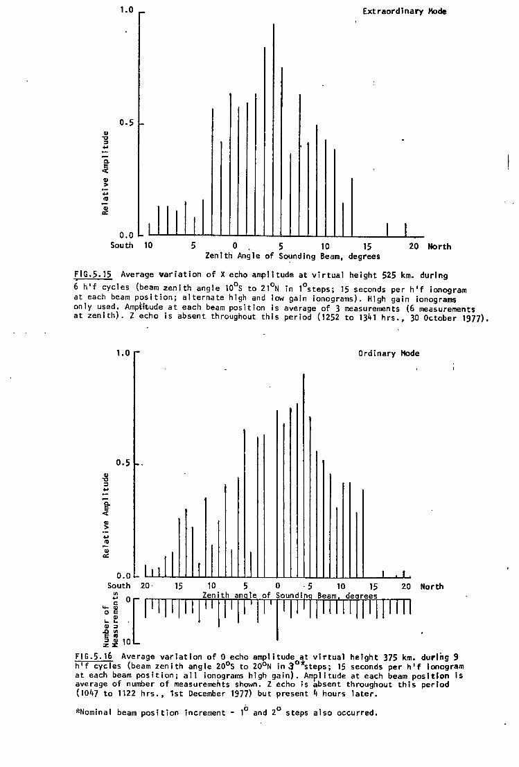
1.0 Extraordinary Hode
o.s G)
"'C :I
. ... 0.. E cc G)
> ... Ill
G) ex:
0.0 I I I I I South 10 5 0 5 10 15 20 North
Zenith Angle of So~ndlng Beam, degrees
FIG.5.15 Average variation of X echo amplitude at virtual height 525 km. during
6 h'f cycles (beam zenith angle 10°s to 21°N in 1°steps; 15 seconds per h'f ionogram at each beam position; alternate high and low gain ionograms). High gain ionograms only used. Amptitude at each beam position is average of 3 measurements (6 measurements at zenith). Z echo is absent throughout this period (1252 to 1341 hrs., 30 October 1977).
1.0 Ordinary Hode
0.5 G)
"'C :I ... 0.. e cc G)
> ... Ill
G) ex:
0.0 I 1 1 l I I l I I
South 20· 15 10 5 0 · 5 10 15 20 North ~ Zenith anrle of Soundinf Beam, derrees
~I°[ 11111111J1
1II1 J 'J 1'I'11 1 111111 11111111
~ ~ 10
FIG.5.16 Average variation of O echo amplitude at virtual height 375 km. during 9 h'f cycles (beam zenith angle 20°s to 20°N in 3°*steps; 15 seconds per h'f lonogram at each beam position; all ionograms high gain). Amplitude at each beam position Is average of number of measurements shown. Z echo is absent throughout this period (1047 to 1122 hrs., 1st December 1977) but present 4 hours later.
*Nominal beam position increment - 1° and 2° steps also occurred.
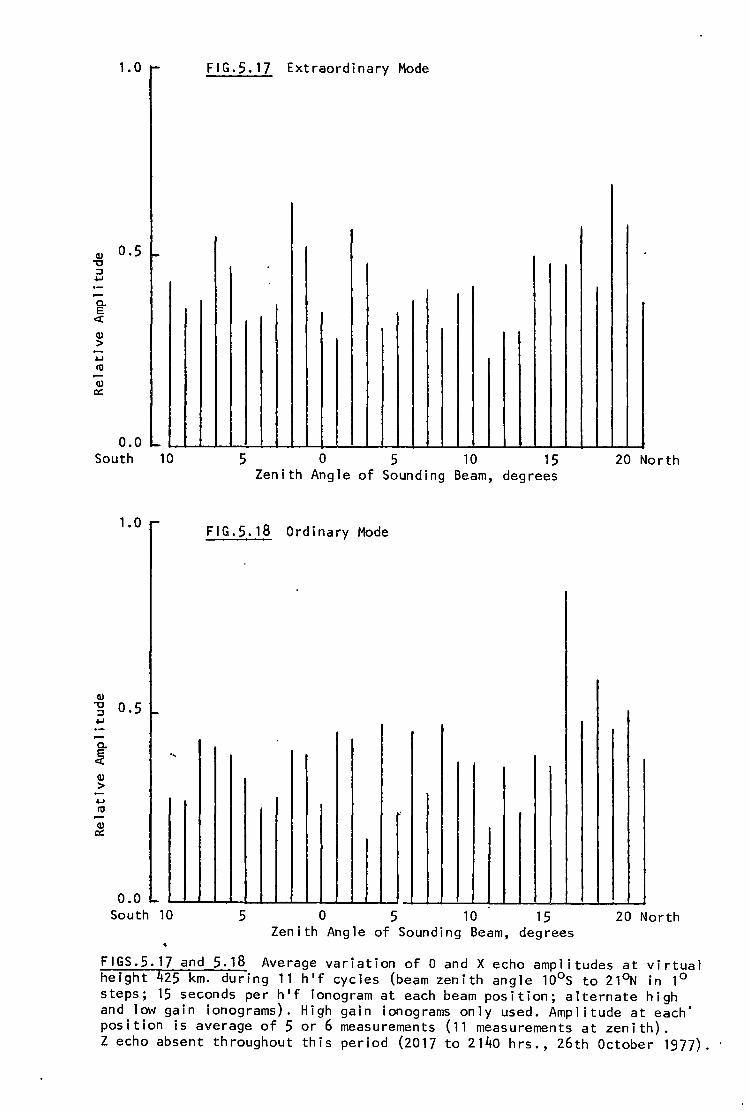
1.0
~ 0.5 -0 ~ µ
~ E ~
~ > µ ro ~ ~
0.0 South 10
~ -0 ~ µ
~ E ~
~ > µ ro ~ ~
1.0
0.5
~
0.0 South 10
FIG.5.17 Extraordinary Mode
5 0 5 10 15 20 North Zenith Angle of Sounding Beam, degrees
FIG.5.18 Ordinary Mode
5 0 5 10 15 20 North Zenith Angle of Sounding Beam, degrees
FIGS.5. 17 and 5.18 Average variation of 0 and X echo amplitudes at virtual height 425 km. during 11 h'f cycles (beam zenith angle 10°s to 21°N in 1° steps; 15 seconds per h'f ionogram at each beam position; alternate high and low gain ionograms). High gain ionograms only used. Amplitude at each" position is average of 5 or 6 measurements (11 measurements at zenith). Z echo absent throughout this period (2017 to 2140 hrs., 26th October 1977).
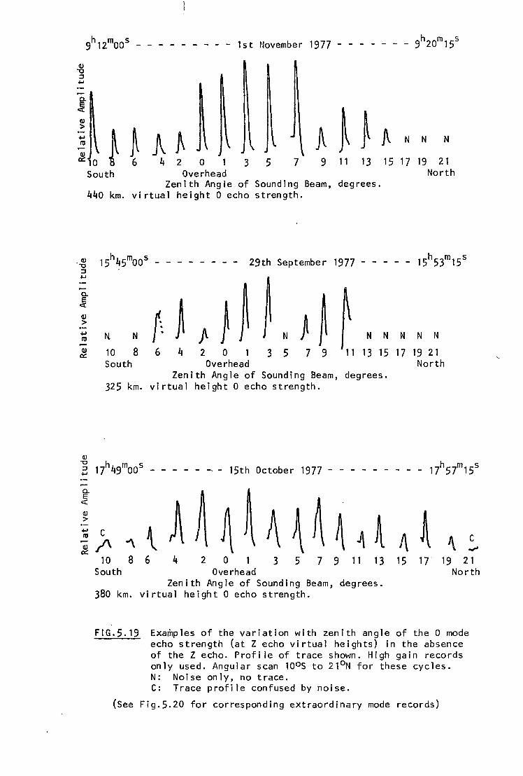
(I) "'C :J .....
~ E <(
(I)
> ..... ltJ
(I) a::
h m s - - - - - 1st November 1977 - - - - - - - 9 20 15
0 } ~ ~ t A 0 3 5 7 9
N N N
11 13 South Overhead
15 17 19 21 North
Zenith Angle of Sounding Beam, degrees. 440 km. virtual height 0 echo strength.
~ E <(
(I)
> ..... ltJ
(I) a::
c.. E
c::(
(I)
> ..... ltJ
(I) a::
h m s 29th September 1977 - - - - - 15 53 15
ij N f: ~ } } N J ~ N N N N N
10 8 6 4 2 0 3 5 7 9 11 13 15 17 19 21 South Overhead North
Zenith Angle of Sounding Beam, degrees. 325 km. virtual height 0 echo strength.
h m s 15th October 1977 - - - - - - - - - 17 57 15
c c /\ "'\ ~A~ ~ ~~A~ ~ A A A '\ ..,.,
10 8 6 4 2 0 3 5 7 9 11 13 15 17' 19 21 South Overhead North
Zenith Angle of Sounding Beam, degrees. 380 km. virtual height 0 echo strength.
FIG.5.19 Examples of the variation with zenith angle of the 0 mode echo strength (at Z echo virtual heights) in the absence of the Z echo. Profile of trace shown. High gain records only used. Angular scan 1oos to 21°N for these cycles. N: Noise only, no trace. C: Trace profile confused by noise.
(See Fig.5.20 for corresponding extraordinary mode records)
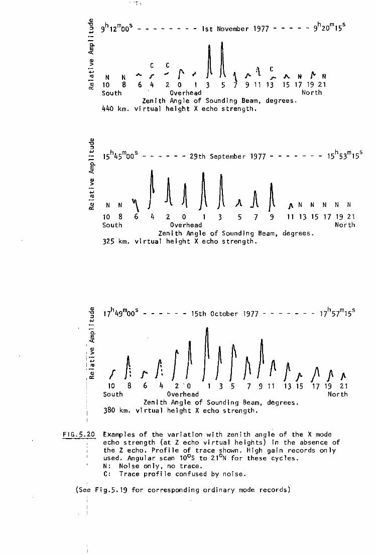
. --.1• •.
h m s 1st November 1977 - - - - - 9 20 15
~
~ ~ <(
Q) > c c ""' I' I'- :\
c t'O N N - r
.,, "' \ /\. N f' N r
Q) 10 8 6 4 2 0 3 5 7 9 11 13 15 17 19 21 a:: South Overhead North
Zenith Angle of Sounding Beam, degrees. 440 km. virtual height X echo strength.
h m s - - - - 29th September 1977 - - - - - - - 15 53 15 0. E
<(
Q)
> .j..I
t'O
Q) a:: N N
10 8 \ } A ~ ~
6 4 2 0 ~ .A A ~ /\ N N N N N
3 5 7 9 11 13 15 17 19 21 South Overhead North
Zenith Angle of Sounding Beam, degrees. 325 km. virtual height X echo strength.
~ 17h49moos - - - - - - 15th October 1977 - - - - - - - 17h57m15s
""' 0. E
<(
Q)
'> ;·-'""' I IO
' It~} J /: f ~ f Q) f r f /\ f' " a::
6 10 8 4 2 ' 0 3 5 7 9 11 13 15 , 7 19 21 South Overhead North
Zen i th Ang 1 e of Sounding Beam, degrees. 380 km. virtual height X echo strength.
FIG.5.20 Examples of the variation with zenith angle of the X mode echo strength (at Z echo virtual heights) in the absence of the Z echo. Profile of trace shown. High gain records only used. Angular scan 10°s to 21°N for these cycles. N: Noise only, no trace. C: Trace profile confused by noise.
(See Fig.5.19 for corresponding ordinary mode records)
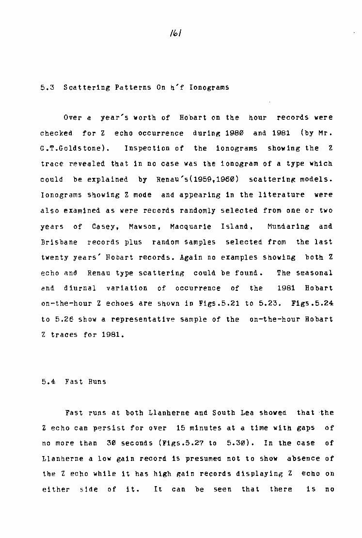
~'
5.3 Scattering Patterns On n'f Ionograms
Over a year's worth of Hobart on the hour records were
checked for Z echo occurrence during 1980 and 1981 (by Mr.
G.T.Goldstone). Inspection of the ionograms showing the Z
trace revealed that in no case was the ionogram of a type which
could be explained by Renau's(1959,1960) scatterin~ models.
Ionograms showing Z mode and appearing in the literature were
also examined as were records randomly selected from one or two
years of Casey, Mawson, Macquarie Island, Mundaring and
Erisbane records plus random samples selected from the last
twenty years' Hobart records. Again no examples showing both Z
echo and Renau type scattering could be found. The seasonal
and diurnal variation of occurrence of the 1981 Hobart
on-the-hour Z echoes are snown in Figs.5.21 to 5.23. Figs.5.24
to 5.26 show a representative sample of the on-the-hour Hobart
Z traces for 1981.
5.4 Fast Runs
Fast runs at both Llanherne and South Lea showed that -the
Z echo can persist for over 15 minutes at a time with gaps of
no more than 30 seconds (Figs.5.27 to 5.30). In the cas~ of
Llanherne a low gain record is presumed not to show absence of
the Z echo while it has high gain records displaying Z echo on
either side of it. It can be seen that there is no
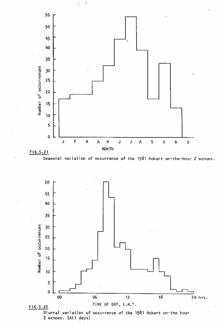
55
50
45
40
35 VI
~ 30 c: Cll I... 25 I... ::I u u 0 20
4-0 I... 15 Cll
..c E ::I z 10
5
0 J
FIG.5.21
I
F M A M MONTH
.
J J
.
A s 0 N D
Seasonal variation of occurrence of the 1981 Hobart on-the-hour Z echoes.
50
45
40.
35
Ill 30 Q) u c: Q)
25 I... I... ::I u u 20 0
4-0
15 I... Q)
~ ::I :z 10
5
0 00 06 12 18
FIG.5.22 TIME OF DAY, L.M.T.
Diurnal variation of occurrence of the 1981 Hobart on-the hour Z echoes. (A 11 days)
' ,
24 hrs.
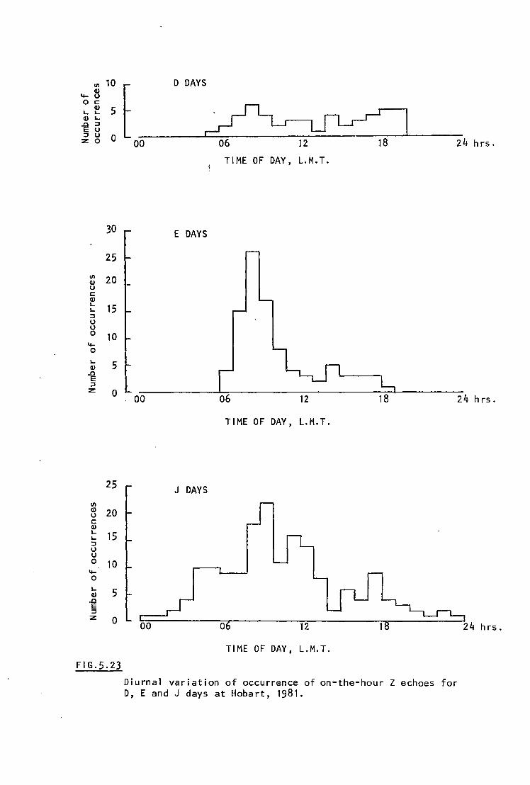
ell 10 (I)
4- 0 0 i::
(I) 5 L. L. (I) L.
~ :J 0
:J 0 0 z 0
30
25
ell 20 Q) 0 c: Q) L.
15 L. :J 0 0 0 10
4-0
L. 5 Q) ..0 E :J z 0
25
ell Q) 20 l) c: Q) L. 15 L. :J 0 l) 0 10
4-0 L. 5 Q)
..0 E :J z 0
FIG.5.23
t D DAYS
~ 00 06 12 18 24 hrs.
Tl ME OF DAY, L.M.T.
E DAYS
00 06 12 18
TIME OF DAY, L.M. T.
J DAYS
00 0 12
TIME OF DAY, L.M.T.
Diurnal variation of occurrence of on-the-hour Z echoes for D , E an d J days at Hob a r t , 19 8 1 .
24 hrs.
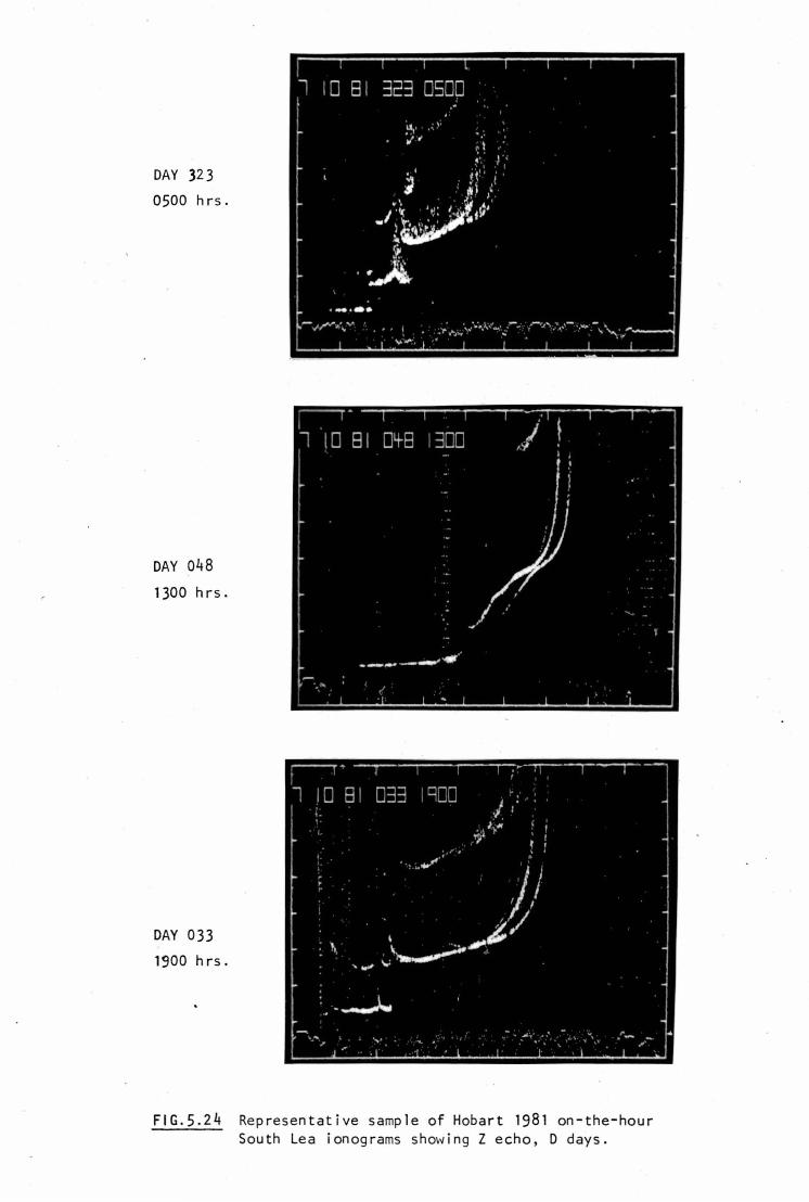
DAY 323 0500 hrs.
DAY 048
1300 hrs.
DAY 033 1900 hrs.
FIG.5.24 Representative sample of Hobart 1981 on-the-hour South Lea ionograms showing Z echo, D days.
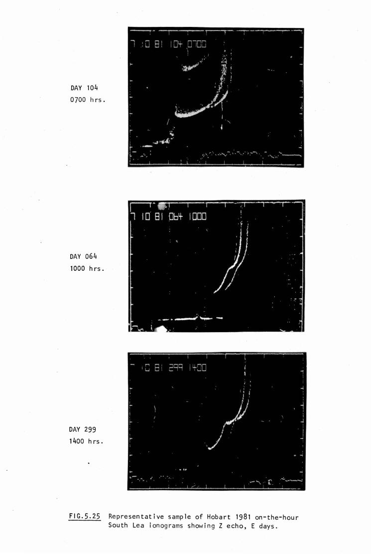
DAY 104
0700 hrs.
DAY 064
1000 hrs.
DAY 299
1400 hrs.
FIG.5.25 Representative sample of Hobart 1981 on-the-hour South Lea ionograms showing Z echo, E days.
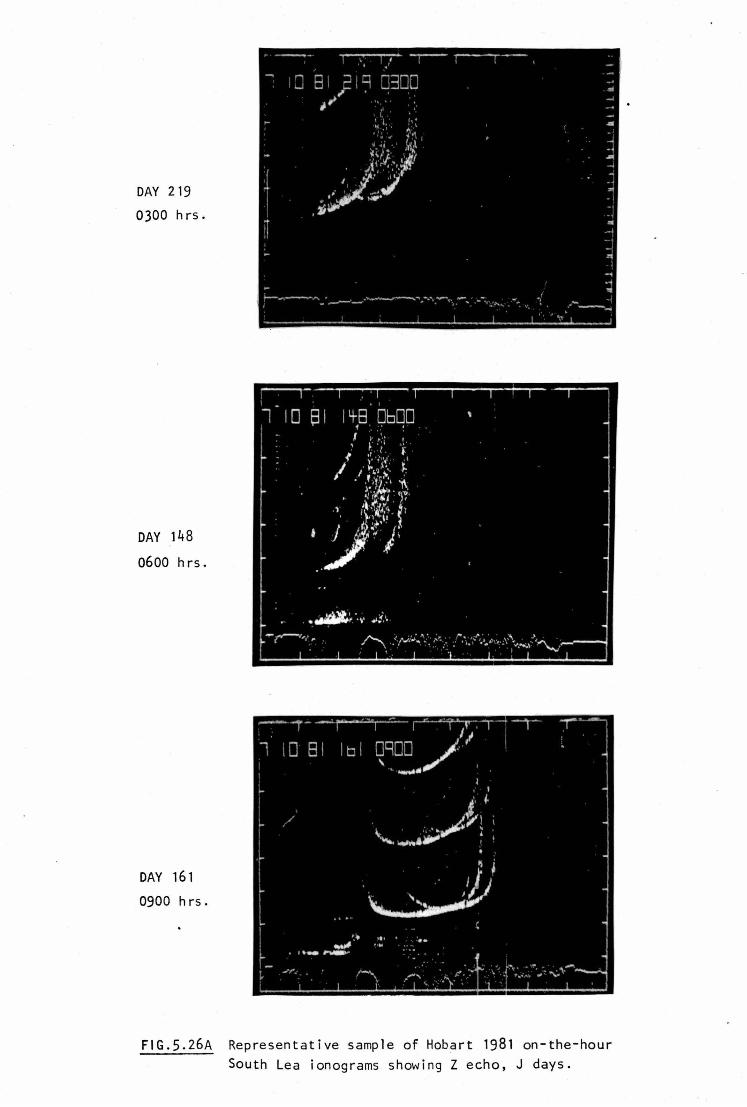
DAY 219
0300 hrs.
DAY 148
0600 hrs.
DAY 161
0900 hrs.
FIG.S.26A Representative sample of Hobart 1981 on-the-hour South Lea ionograms showing Z echo, J days.
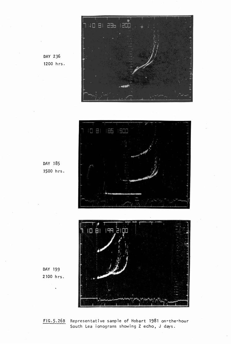
DAY 236
1200 hrs.
DAY 185
1500 hrs.
DAY 199
2100 hrs.
FIG.5.268 Representative sample of Hobart 1981 on-the-hour South Lea ionograms showing Z echo, J days.
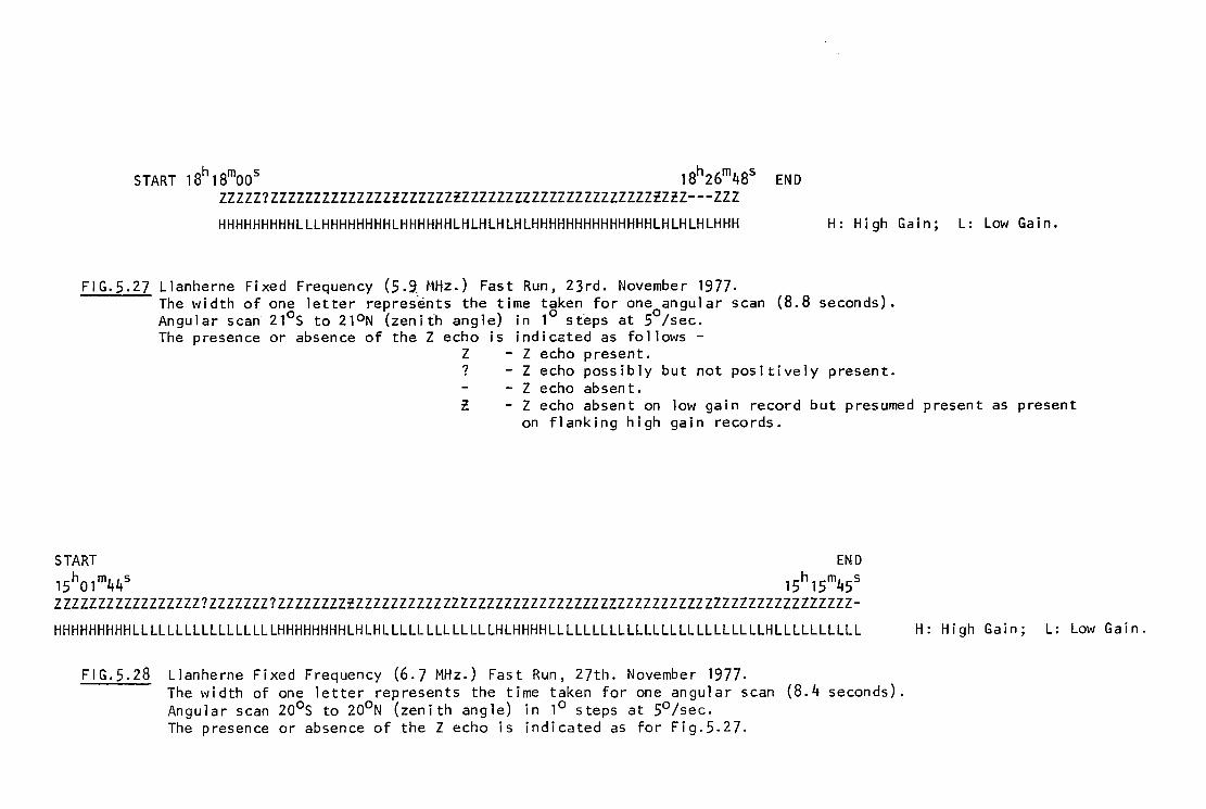
START 18h 18mOOs 18h26m48s END ZZZZZ?ZZZZZZZZZZZZZZlZZZZZZlZZZZZZZZZZZZZZZZZZZZZZlllZ---zzz
HHHHHHHHHLLLHHHHHHHHLHHHHHHLHLHLHLHLHHHHHHHHHHHHHHLHLHLHLHHH H: High Gain; L: Low Gain.
FIG.5.27 Llanherne Fixed Frequency (5.9_ MHz.) Fast Run, 23rd. November 1977. The width of one letter represents the time taken for one angular scan (8.8 seconds). Angular scan- 21°s to 210N (zenith angle) in 1° sfeps at 5°/sec. The presence or absence of the Z echo is indicated as follows -
Z - Z echo present. ? - Z echo possibly but not positively present.
- Z echo absent. l - Z echo absent on low gain record but presumed present as present
on flanking high gain records.
START END 15ho1m44s 15h15m45s ZZZZZZZZZZZZZZZZZ?ZZZZZZZ?ZZZZZZZZlZZZZZZZZZZZZZZZZZZZZZZZZZZZZZZZZZZZZZZZZZZZZZZZZZZZZZZZZZ-
HHHHHHHHHLLLLLLLLLLLLLLLLLHHHHHHHHLHLHLLLLLLLLLLLLLHLHHHHLLLLLLLLLLLLLLLLLLLLLLLLLHLLLLLLLLLL
FIG.5.28 Llanherne Fixed Frequency (6.7 MHz.) Fast Run, 27th. November 1977. The width of one letter represents the time taken for one angular scan (8.4 seconds). Angular scan zo0s to zo0N (zenith angle) in 1° steps at 5°/sec. The presence or absence of the Z echo is indicated as for Fig.5.27.
H: High Gain; L: Low Gain.
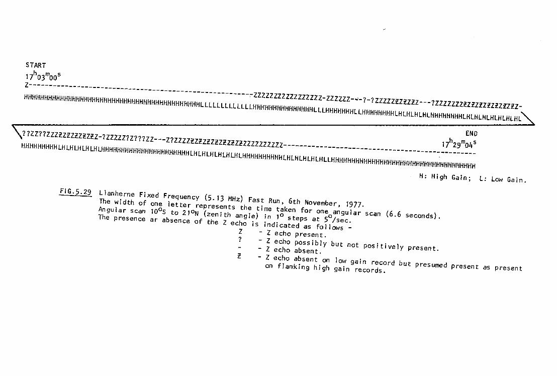
START
17h03m00s
z-------------------------------------------------------czzzzzzzzzzzzzzzzz-zzzzzz-•-1-1zzzzzzzzzzz---1zzzzzzzzz'lZiZiZiZiZlZHHHHHHHHHHHHHHHHHHHHHHHHHHHHHHHHHHHHHHHHHHHHLLLLLLLLLLLLLHHHHHHHHHHHHHHHLLLHHHHHHHLLHHHHHHHHLHLHLHLHLHHHHHHHHLHLHLHLHLHLHLHL
17h29m04s 11ZZ?1ZZZiZiZlliZiZ-1ZZZZZ1Z1?1ZZ---z1zzzzzzzziZiZiZiZiZZZZZZZZZZ------------------------------------------------
HHHHHHHHHLHLHLHLHLHLHHHHHHHHHHHHHHHHHHHHHHLHLHLHLHLHLHLHHHHHHHHHHLHLHLHLHLHLLHHHHHHHHHHHHHHHHHHHHHHHHHHHHHHHHHHHH
END
H : H i gh Gain ; L : Low Ga i n .
FIG.5.29 Llanherne Fixed Frequency (5. 13 MHz) Fast Run, 6th November, 1977.
The width of one letter represents the time taken for one angular scan (6.6 seconds). Angular scan 10°s to 21°N (zenith angle) in 1° steps at 5°/sec. The presence ar absence of the Z echo is indicated as follows -
Z - Z echo present.
? - Z echo possibly but not positively present. - Z echo absent.
~ - Z echo absent on low gain record but presumed present as present on flanking high gain records.
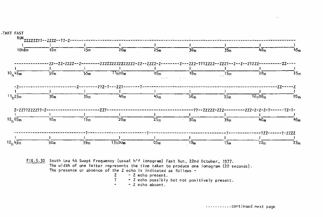
··TART FAST
RUNZZZZZZ77--ZZZZ--77-Z-------------------------------------------------------------------------------------------------I I I I I I I I I
1 Oh6m 1 Om 15rrr - - 20m 25m 30m 35m 40m 45m
---------------zz--zz-zzzz--z--------zzzzzzzzzzzzzzz-zz--zzzz-z--------z---zzz-111zzzz--zzz1--z--z--z1zzz----------zz----1 I I I , I I I I I
10h 45m 50m 55m llhOOm 05m 10m 15m 20m 25m
-z-------------------------z--------11z-1---zz1-------1----------------------------------------------------------zz-----z I ____________ 1 _______ 1 _______ 1 ______________ 1 ______ 1 _____ _
11h25m 30m 35m 40m 45m 50m 5.5m 12h00m 05m
Z-ZZ77ZZZZ77-Z-----------------------ZZ?-------------------------------------77--ZZZZZ-ZZZ---------zzz-z-z-z-7------7Z-7-I I I I I I I I I
12h OSm 10m '15m '20m 'Z5m 30m 35m 40m 4Sm
-------------------------------7-------------------------?---------------------------------?--------------?ZZ------?-ZZZZ I I I I I I I I I
12h45m 50m 55m 13h0Um 05m 10m 15m 20m 25m
FIG.5.30 South Lea 4A Swept Frequency (usual h 1 f ionogram) Fast Run, 22nd October, 1977. The width of one letter represents the time taken to produce one ionogram (20 seconds). The presence or absence of the Z echo is indicated as follows -
Z - Z echo present. ? - Z echo possibly but not positively present.
- Z echo absent.
. .......... continued next page
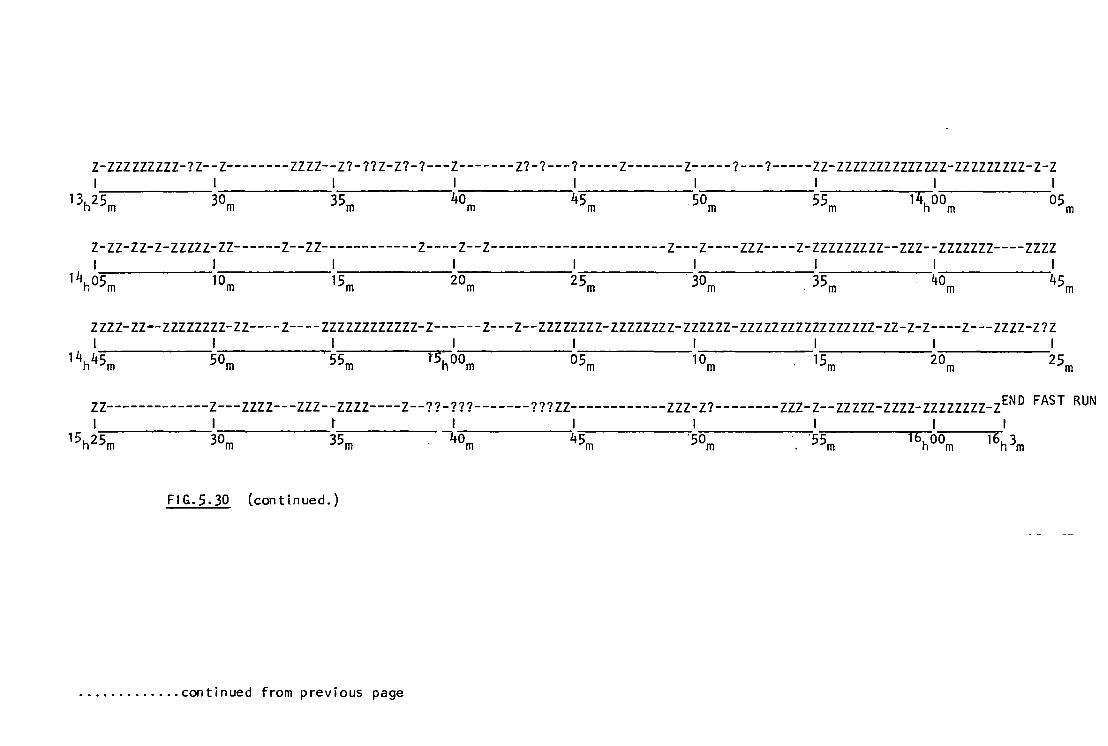
z-zzzzzzzzz-1z--z--------zzzz--z?-??z-z1-1---z-------z1-1---1-----z-------z-----1---1-----zz-zzzzzzzzzzzzzz-zzzzzzzzz-z-z I I I I I I I I I
13h25 30m 35 40 45 . 50 55 14hoo 05 m m m m m m m m
z-zz-zz-z-zzzzz-zz------z--zz------------z----z--z----------------------z---z----zzz----z-zzzzzzzzz--zzz--zzzzzzz----zzzz I I I I I I I I I
14ho5m 10m 15m 20m 25 30 35 40 45 m m · m m m
zzzz-zz·-zzzzzzzz-zz----z----zzzzzzzzzzzz-z------z---z--zzzzzzzz-zzzzzzzz-zzzzzz-zzzzzzzzzzzzzzzzz-zz-z-z----z---zzzz-z?z I I I I I I I I I
14h45m 50m 55m t5hoom 05m 10m . 15m 20m 25m
zz-------------z---zzzz---zzz--zzzz----z--11-111-------111zz------------zzz-z1--------zzz-z--zzzzz-zzzz-zzzzzzzz-zEND FAST RUN
FI G. 5. 30 (continued. )
............. continued from previous page
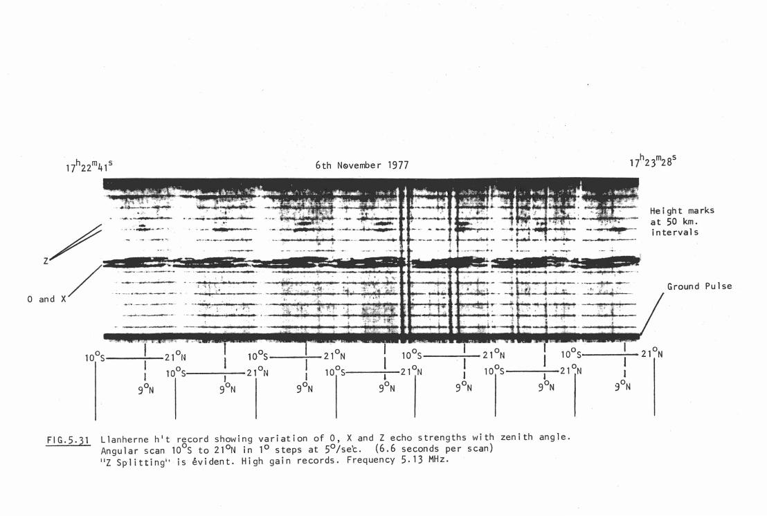
FIG.5.31
6th N~vember 1977
• ' I
.. - 1 ·t { ( .... : ., , :~ . ,
' .! ""1~ -f\!; ' ; .-.::\; ~ t-:.. if, ,_4. 'j
. l f
.. .. • t~ ......
'
I 21°N 10°5 I 21°N 10°5 I 10°5 21°N I 10°5 21°N I l I I
9°N 9°N 9°N 9°N
Llanherne h 1 t record showing variation of 0, X and Z echo strengths with zenith angle. Angular scan 10°5 to 21°N in 1° steps at 5°/set. (6.6 seconds per scan) 11 z 5p·litting1• is evident. High gain records. Frequency 5.13 MHz.
I I l
9°N
Height marks at 50 km. intervals
Ground Pulse
21°N
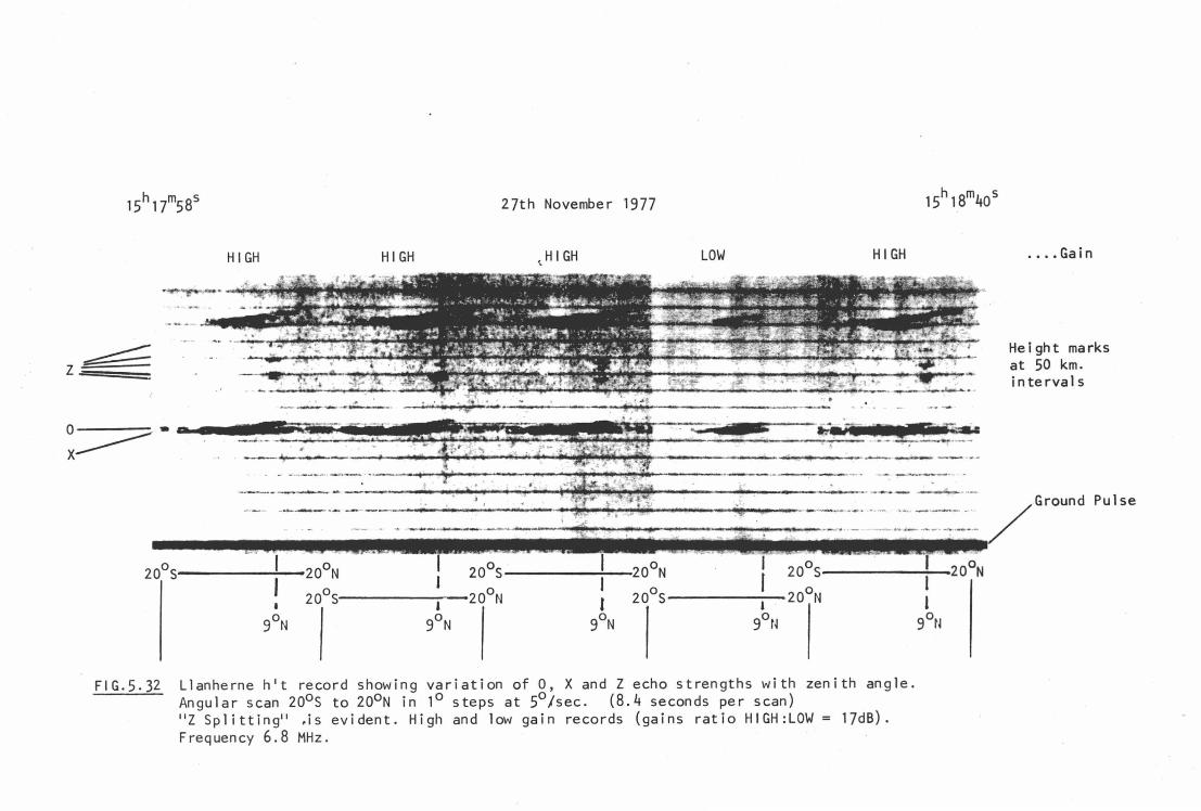
27th November 1977
HIGH HIGH ~HIGH LOW HIGH
~------· ··=~~~, ~~~~~~~~!!!:9!!!1!t=:.-~·~-~-s~~ • _____ ...,..~ ...... ..__....._.._.....:.NI ..... ~ ............. __________ . ______ ..._____. ... _ ·--
20°s----...:.'-20°N : 20°s----..:..!-20°N : 20°s . : 20°N
! 20°s------1-20°N 1 20°s-----1-20°N 1
9°N 9°N 9°N 9°t~ 9°N
FIG.5.32 Llanherne h't record showing variation of 0, X and Z echo strengths with zenith angle. Angular scan 20°s to 20°N in 1° steps at 5°/sec. (8.4 seconds per scan) 11 Z Splitting" .is evident. High and low gain records (gains ratio HIGH:LOW = 17dB). Frequency 6.8 MHz.
.... Gain
Height marks at 50 km. in terva 1 s
Pulse
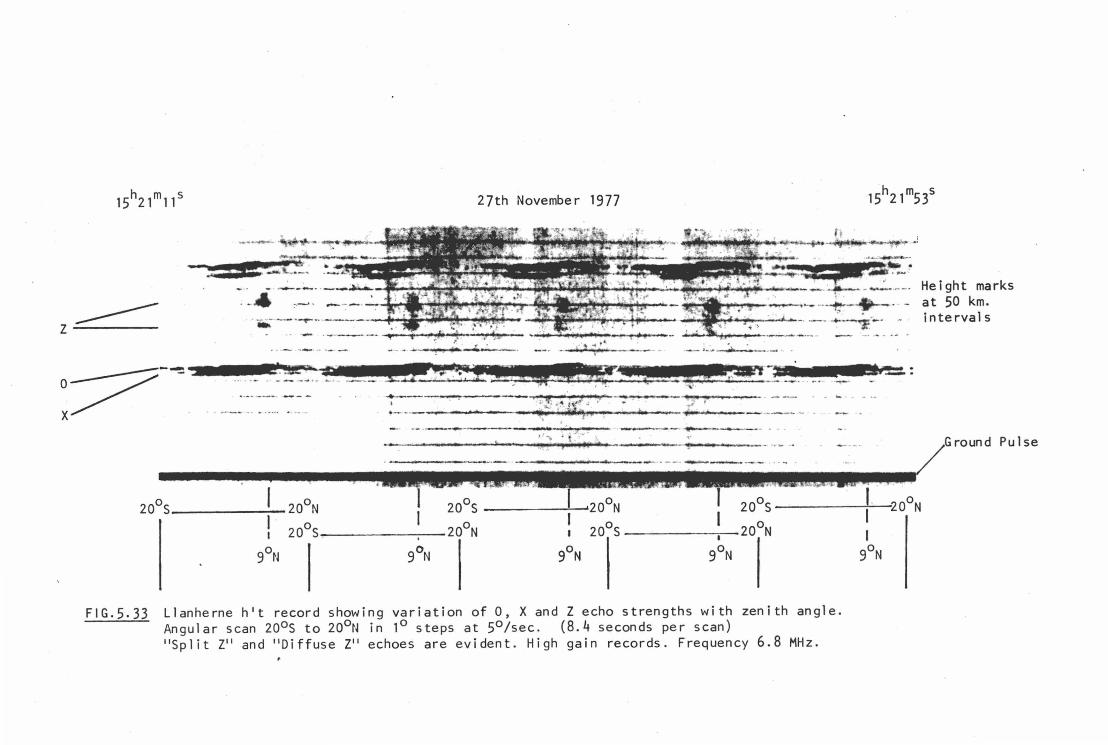
z -------
I
27th November 1977
··-· - - IT~~:~ ._1 _ £~:•..,:~!"JE_ i 4!J , 41 ,dl' ,~· ·NJJ -. ·---· . - - - -------- .. ---..- _ . ...,...__.._..,__.__ ~
__ ___ _ __... _ _ "'!'!""_,, ....... ...--...----~-....... --- .. ~ -
------------·-·-- ........._- .. .. --- .. .. .
Height marks at 50 km. intervals
J
I
/Ground Pulse
...... ~ ............ ~. za•••••na .. a•1•ct•1••:~11•a.,m11111£1U111111Mam11111i! .. 12•z .. •2•sa•1•t~c~11•c~i•: ... • I 20°s I 20°N I 20°s I 20°s 20°N
I 20°s . I I I I I
~-----~20°N 20°s 20°N
9°N
FIG.5.33 Llanherne h't record showing variation of 0, X and Z echo strengths with zenith angle. Angular scan 20°s to 20°N in 1° steps at 5°/sec. (8.4 seconds per scan) "Split z11 and 11 Diffuse z11 echoes are evident. High gain records. Frequency 6.8 MHz.
115
quasi-periodicity such as that found in TID's. The Z echo is
also seen to change its strength markedly within periods much
less than a minute.
5.5 Z Splitting
On two days the Z echo was observed on Llanherne swept
zenith angle h't records to split into two or more echoes and
the phenonemon would be that described by Bowman,(1960) as
z-ray trace duplication and found by him on 2 percent of the
Hobart records which he examined (five months of 1946).
Figs.5.31 to 5.33 show examples of Z splitting and Fig.3.25A(e)
shows an example found by Bowman. Some of the Z echoes of
Fig.5.33 are seen
well correspond to
Fig.3.25A(f).
to have a diffuse appearance and these may
Bowman's "diffuse z-ray", illustrated by
6.1 Introduction
CHAPTER SIX
DISCUSSION
Very little discussion of the results is required.
Consideration of the discussion sections of Chapter Three and
the aims and results of the experiments quickly leads us to the
conclusion that none of the theories so far advanced offers an
adequate Z ray return explanation for the vast majority of Z
echo occurences.
6.2 Solar Zenith Angle Tilt Theory
No Z echo angles of arrival of +18° were observed at any
time of day even when strong 0 and X echoes occurred at Z echo
virtual heights at zenith angles around +18° (implying that the
ionosphere as a wnole was not tilted by 18°). This theory
fails to explain the +8/9° angle of arrival of the Z echo and
even smaller angles of arrival (of the centre of the angular
distribution) of the 0 and X echoes. It is safe to discard
this theory except for possible special cases as outlined in
section 3.8.
111
6.3 Backscatter Theory
There were found no h'f ionograms displaying the required
scattering patterns. Furthermore, the 0 and X angular profiles
were not noticeably increased on average during the presence of
the Z echo (apart from the secondary peak mentioned in the
previous chapter and this is not easily attributable to
backscattering - this feature in any case persisted durinR
periods of absence of the Z echo). This theory also awaits a
satisfactorily detailed theoretical explanation which has not
as yet been forthcoming. It would be safe to discard this
theory as a general Z echo explanation though it is of course
still possible that it could be required to explain odd,
isolated cases.
6 .4 Tilt Theory
The tilt theory predicts that the centre of the Z mode
angular return spectrum will have values in the general range
+ge to +18° with an expected very strong bias toward values
between +14° and +17° (and·
possibilty of values less than
only the sliRhtest practical
" +9 ). That this theory would
fail the Z echo angle of arrival test so dramatically is to be
expected from Ellis's (1953a,b;l956) results which are here
confirmed. Nevertheless, it would be possible to construct a
tilt model which would return t~e Z echo at +9° although it is
118
most improbable that this model could occur in every case
(furthermore Papagiannis and Miller's 1969 results indicate
that the (frequency) spectral range from such a model would be
unrealistically narrow as b would need to be relatively large
and a so small as to be insignificant). Given that this model
has been operating in each of our observed cases then the O and 0 X beam centres should also be at +9 • This was observed in one
instance only (Fig.5.12). This instance might be a sole
example of a tilt mechanism operating although the relatively
large (frequency) spectral range (0.4! 0.05 MHz.) of the Z echo
on the simultaneously {1545 nrs.) recorded South Lea h'f
ionogram suggests not (see Fig.3.41).
Although unlikely, it is conceivably possible that when
Llanherne h'f sounding was in progress there existed a dynamic
ionosphere such that flat ionospheric layers were nearly
overhead when the sounding beam was near zenith and that
favourable tilt/wedge layers occurred in the corrP.ct part of
the sky for Z ray return by the ti~e (say, 2 minutes later) the
sounding beam reached +8/9°. Travelling ionospheric
disturbances (TID's) travelling along the magnetic meridian
might provide such a situation. However, if this were to be
the case, the expected
narrower (as angles
Z echo frequency spectrum would be far
of arrival are around +8/9°) t~an that
observed. Secondly the Z echo could only appear for say 5% (at
a very generous estimate) of the quasi-period of the ~ID. This
makes the commonly observed appearanc~ of the Z echo on
successive cycles unlikely; but again it is
What is not possible with such a mechanism,
remotely possible.
however, is t~e
persistent presence of the Z echo for relatively long periods
with only relatively short breaks (this typical Z echo
behaviour may be seen in the fast run results of Figs.5.27 to
5.30).
The tilt
occurrence on a
theory fairly clearly
global basis. It may
fails to explain Z mode
perhaps be expected to
have some application on a routine basis at very high dip
angles but it has not explained the Z echoes at a station of
relatively high Z echo incidence and it might be expected to
have even less applic~tion at stations such as Allahabad where
Z echoes are regularly if infrequently seen and the dip angle
is only 36°.
6.5 Conclusions
Since the current Z echo return mechanisms are unable to
explain the observed results we must search for a more
satisfactory pro~osition. Consideration of both experiment and
theory suggests that it would be desirable to have a mechanism
with a satisfactory physical process (as with the tilt theory)
but which leaves the ionosphere unperturbed on an overall scale
(as with the backscatter theory and in line with experimental
results). A further desired feature of such a mechanism would
180
be a measure of natural selectivity as far as the Z
concerned so that contrive~ ionospheric distributions
mode is
(as with
the tilt theory) are not required and the mere presence of the
phenomenon is sufficient to return the Z echo. As is
illustrated by the experimental results, the Z ray return
mechanism must also be able to operate irrespective of (and not
because of) tilts in the ionosphere. An attempt to develop
such a mechanism is presented in the following chapter.
CHAPTER SEVEN
THE Z DUCT RETURN MECHANISM
7.1 Introduction
Section 7.2 introduces an alternative Z
mechanism. Section 7.3 describes some computer
the mechanism. Further sections examine available
an explanation for Z splitting is given.
7.2 The Z Duct Model
ray return
modelling of
evidence and
Consider a horizontally stratified ionosphere upon which
is superimposed a column of depletion of electron density or
duct. Allow this column to be field aligned and to extend from
the peak of the F2 layer downwards at least as far as the X = 1
level. The column may extend an arbitrary distance upwaras
from the peak electron density layer as this will not concern
us. Let the column have a maximum depletion (along its axis)
of less than, say, one percent of the ambient electron aensity,
let the depletion cross section of the column be sinusoidal and
let the width of the column be 10 to 100 wavelengths. Consider
an O mode wave emitted at such an angle by a ground transmitter
that on reaching the X = 1 level it has its wave normal
parallel to the magnetic field. Around this ray there will be
182
a small cone of rays which make a slight angle (say, less than
half a degree) with the magnetic field line. This is the cone
of rays which (for this particular frequency) will generate the
upper extraordinary or
this transmitter will
Z mode and no otner cone generated by
have this property. Allow the X = 1
point for this ray cone to fall on the axis of the column of
depletion. The longitudinal ray emerging upwards from the
coupling zone will propagate along the axis of the column
without deviation as its wave normal will be perpendicular to
the on axis ionization contours (unless the duct is very weak).
It will be guided upwards alon~ the magnetic field line until
the ionization density becomes such that X = 1+Y where it will
be normally reflected and the reflected ray will be guided back
down the column to the coupling point where its energy will be
converted back to 0 mode and it returns to the transmitter - a
Z echo. Other rays in the cone which make small angles .wita.
the magnetic field line will travel out towards the sides of
the column but in doing so they will be travelling into
laterally as well as vertically increasing electron densities
and thus may be turned back towards the centre of the column.
These rays may be contained within the column, guided up along
the magnetic field line to the X ~ l+Y reflection point wbere
they will be guided back down the column to the couplin~
region. If the rays make too great an angle with the magnetic
field direction then tney will penetrate the walls of t~e
colu111n and
coupling
escape. However Z
region necessarily
rays emerging upwards
make very small angles
from the
with the
/83
magnetic field direction and thus the column may be quite weak
(in depletion) yet trap most of the Z mode energy by virtue of
its field alignment. Such a column tGerefore behaves as a duct
for Z echoes. The column is also capable of ducting 0 and X
mode rays whicn enter the duct with their wave normals parallel
or nearly parallel to the axis. A trapped 0 mode can be
expected to have most of its energy converted to the Z mode.
The O mode and X mode energy trapped by the duct represents
only a very small fraction of the 0 and X energy transmitted
but the Z mode energy trapped may represent almost all the Z
energy transmitted. We thereby have a Z return mechanism which
returns the Z energy back along its path by normal total
reflection and which furthermore displays great selectivity
towards the Z mode. Since the ducts may be quite weak the
ionosphere remains essentially unchanged as required and
overhead X and O echoes are returned from the host ionosphere
vertically as usual if it is flat or obliquely from the
appropriate off zenith angle if it is inclined. As with tne
Backscatter Model, the heavy restrictions on electron density
configuration required by the Tilt Model do not apply. At the
same time we have the advantage of tne well known p~ysical
reflection process of the Tilt Model. High in the F2 layer
where the sides of the duct become steeper (in the sense that
the ionization contours make smaller angles Jith the magnetic
field direction) it would be expected that the presence of the
ducts ~ould assist the return of some oblique O and X rays
travelling externally to the ducts. This might explain the
secondary peak noted in section 5.2 and the results of
Ellis's experiment discussed in section 3.4 (Fig.3.12).
The duct model has been described very simply and appears
to show great promise as a possible Z ray return mechanism but
we must now examine it in more detail to check that it can in
fact behave as outlined.
7.3 Computer Ray Tracing
Computer ray tracing of the Z mode in a flat ionosphere
with superimposed ducts was carried out using the Jones (Jones
and Stephenson,1975) ray tracing routines as the core of the
program. Jones did not design the program for this sort of
work but made it sufficiently versatile to be aaaptable for
many needs. Tracing the Z ray near the coupling region by
itself calls for some care but the additional complication of
high and spatially quickly varying lateral ionisation gradients
(when ducts are introduced) means that not only is the program
operating about an extreme edge of its ability but further that
the assumptions of geometrical ray tracing may sometimes be
violated to a greater or lesser degree. The ionosphere was
~odelled as parabolic of half thickness 150 km. and maximum
electron density 300000 electrons/cc. The dip angle was taken
as ?2° (Hobart) and a standard earth-centred dipole field was
employed. Lateral sinusoidal electron density variations were
l'lS
superi~posed on the ionosphere and a height dependent phase
term introduced so that ducts were for~ed parallel to the
magnetic field direction. Collisions were neglected. The Z
ray was started from a tttransmitter" just above the coupling
region, the wave and group normals being (unrealistically,
except at the coupling point itself) set in the magnetic field
direction and up to nalf a degree eitner side. The maximum
step length of the ray tracing was generally set to 0.5 km. In
view of all the assumptions and approximations the model must
be regarded
accordingly.
as
It
possibly crude
had been hoped
and tne
firstly
results interpreted
to establish that
trap~ing could take place and secondly to establish trapping
criteria.
In order to establish that successful trapping had taken
place in the model, two requirements were set. The first was
that used by Papagiannis and Miller (19B9) to test t~e
til/wedge theory: namely that the ray return to the same
physical point in space. The second requirement was that the
ray be able to couple to an 0 mode on its return to the
coupling region. Printed output from the program provided
unambiguous information on the first requirement and some ray
path plotting was done but very little value is gained from
these plots without greatly exag~erating the scale transverse
to the duct axes. Printed output information on the second
requirement was not easily interpreted and so the ray's
progress was plotted on a Poeverlein diagram. this ~roviding
/86
more information and a much clearer picture of the ray's
behaviour than a plot of its physical path·. Successful ray
trapping was achieved in a variety of duct models, with widths
ranging from 1.5 to 7km. and electron density deviations from
ambient (A N/N) of 5% to 0.1% thougn not all combinations were
tried and not all those combinations which were tried were
successful. Rays outside tne coupling cone were not
investigated as they would automatically fail the second
requirement since tney could not start at the upward coupling
region of the Poeverlein diagram. Despite the rays which did
fail to return and despite the approximate nature of the model
it was concluded that the validity of Z ducts as a return
mechanism was reasonably well established (in as far as models
can establish validity), especially considering that error
buildup was likely to make the program turn the ray away from
the coupling region rather than towards it. Fig.7.1 is a
diagram explaining the Poeverlein plots, Figs.7.2 to 7.8 show
trapping situations and Fig.7.9 shows a non trapping situation.
Figs.?.10 and 7.11 are plots of the physical ray paths in tne
ionosphere.
Unfortunately trapping criteria could not be established
from the modellin~ results. Certainly there were results which
could have been analysed but it was felt that such an analysis
could be at best meaningless and at worst misleatting. For many
duct models, trapping conditions could be altered to
non-trap~ing situations by relatively minute variations in such
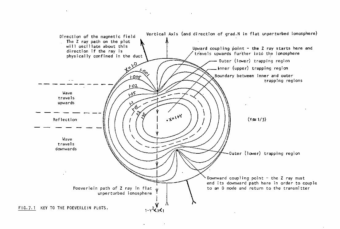
FIG. 7. 1
Direction of the magnetic field The Z ray path on the plot wil I oscillate about this direction if the ray is physically confined in the
Vertical Axis (and direction of grad.N in flat unperturbed ionosphere)
Wave travels upwards
Reflection
Wave travels
downwards
Poeverlein path of Z ray in flat w unperturbed ionosphere ?
I KEY TO THE POEVERLEIN PLOTS. 'f
1-v2<x<1
coupling ~oint - the Z ray starts hare and upwards further into th~ ionosphere
Outer (lower) trapping region
~nner (upper) trapping region
inner and outer trapping regions
(Y~ 1/3)
Outer (lower) trapping region
Downward coupling point - the Z ray must end its downward path here in order to couple to an 0 mode and return to the transmitter
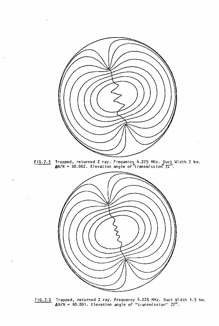
FIG.7.3 Trapped, returned Z ray. FrequencY. 4.225 MHz. Duct Width 2 km. AN/N = ±0.002. Elevation angle of"transmissio~72°.
FIG.7.2 Trapped, returned Z ray. Frequency 4.225 MHz. Duct Width 1.5 km. ~N/N = ±0.001. Elevation angle of 11 transmission 11 72°.
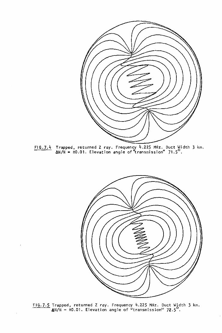
FIG.7.4 Trapped, returned Z ray. Frequency 4.225 MHz. Duct Width 3 km. 6N/N = ±0.01. Elevation angle of 11transmission" 71.5°.
FIG.7.5 Trapped, returned Z ray. Frequency 4.225 MHz. Duct Width 3 km. AN/N = ±0.01. Elevation angle of ~ 1 transmission 11 72.5°.
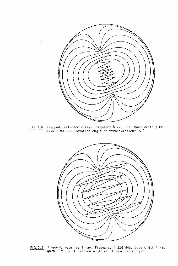
FIG.7.6
FIG.7.7
Trapped, returned Z ray. Frequency 4.225 MHz. Duct Width 3 km. AN/N = ±0.01. Elevation angle of 11 transmission 11 72°.
T~apped, returned Z ray. Frequency 4.225 MHz. Duct Width 4 km. AN/N = ±0.05. Elevation angle of 11 transmission 11 72°.
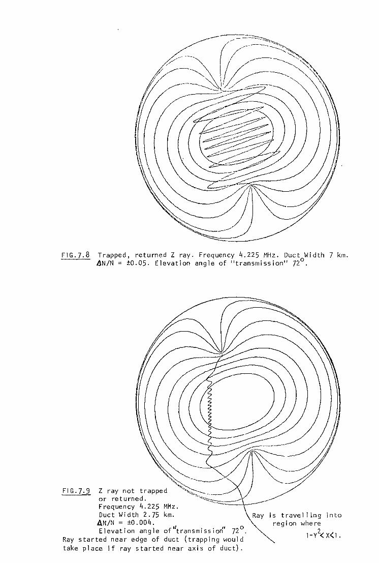
FIG.7.8 Trapped, returned Z ray. Frequency 4.225 MHz. Duct Width 7 km. L}N/N = ±0.05. Elevation angle of 11 transmission 11 72°.
\, '>~
d "' FIG.7.9 Z ray not trappe ""'-~-------or returned. ·--~.:::.~ ___ .....-Frequency 4.225 MHz. -----·~--.\--~
Duct Width 2.75 km. AN/N = ±0.004. E l • l f II • • II 72 0 evat1on ang e o transm1ss1on .
Ray started near edge of duct (trapping would take place if ray started near axis of duct).
is travel ling into region where
1-v2<x<1.
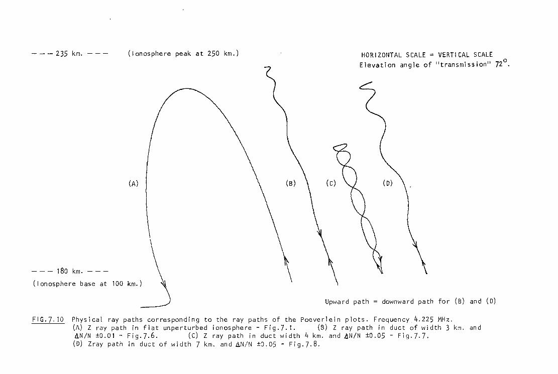
---235 km. --- (Ionosphere peak at 250 km.)
(A)
--- 180 km. --
(Ionosphere base at 100 km.)
HORIZONTAL SCALE= VERTICAL SCALE Elevation angle of 11 transmission 11 72°.
Upward path = downward path for (B) and (D)
FIG.7. 10 Physical ray paths corresponding to the ray paths of the Poeverlein plots. Frequency 4.225 MHz. (A) Z ray path in flat unperturbed ionosphere - Fig.7. 1. (B) Z ray path in duct of width 3 km. and 4N/N ±0.01 - Fig.7.6. (C) Z ray path in duct width 4 km. and 4N/N ±0.05 - Fig.7.7. (0) Zray path in duct of width 7 km. and dN/N ±0.05 - Fig.7.8.
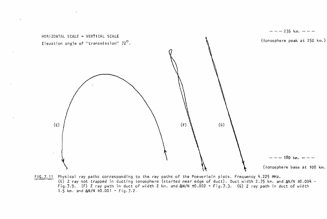
HORIZONTAL SCALE= VERTICAL SCALE
Elevation angle of 11 transmission 11 72°.
( E)
- - - 235 km. - - -
(Ionosphere peak at 250 km.)
- - - 180 km. - - -
(Ionosphere base at 100 km.
FIG.]. 11 Physical ray paths corresponding to the ray paths of the Poeverlein plots. Frequency 4.225 MHz. (E) Z ray not trapped in ducting ionosphere (started near edge of duct). Duct width 2.75 km. and AN/N ±0.004 -Fig.7.9. (F) Z ray path in duct of width 2 km. and AN/N ±0.002 - Fig.7.3. (G) Z ray path in duct of width 1.5 km. and AN/N ±0.001 - Fig.].2.
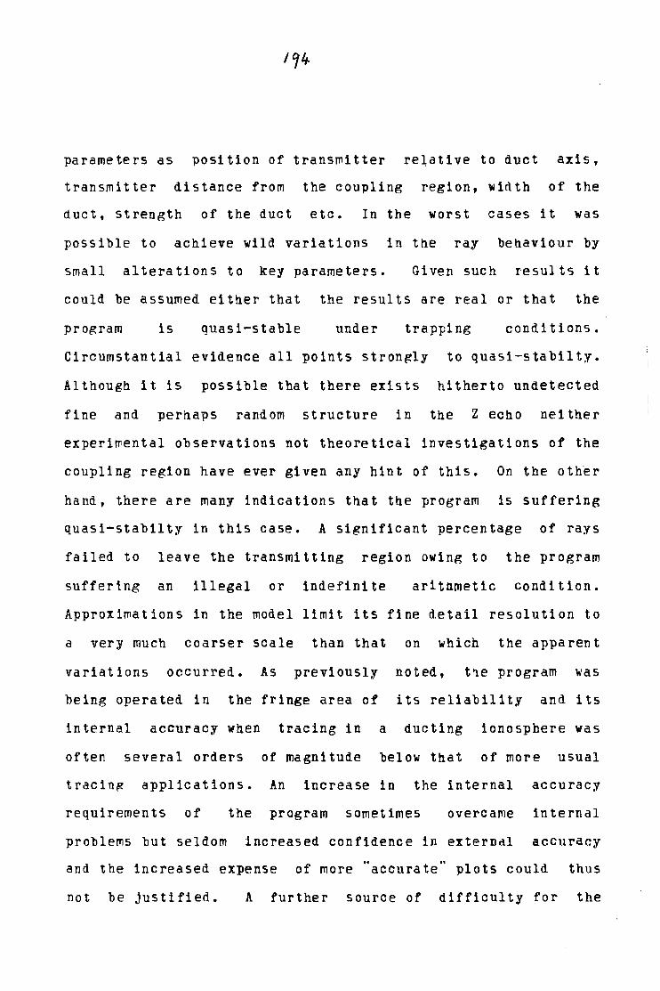
parameters as position of transmitter re~ative to duct axis,
transmitter distance from the coupling region, width of the
duct, strength of the duct etc. In the worst cases it was
possible to achieve wild variations in the ray behaviour by
small alterations to key parameters. Given such results it
could be assumed either that the results are real or that the
program is quasi-stable under trapping conditions.
Circumstantial evidence all points strongly to quasi-stabilty.
Although it is possible that there exists hitherto undetected
fine and perha~s random structure in the Z echo neither
experi~ental observations not theoretical investigations of the
coupling region have ever given any hint of this. On the oth~r
hand, there are many indications that the program is suffering
quasi-stabilty in this case. A significant percentage of rays
failed to leave the transmitting region owing to the program
suffering an illegal or indefinite arithmetic condition.
Approximations in the model limit its fine detail resolution to
a very much coarser scale than that on which the apparent
variations occurred. As previously noted, t~e program was
being operated in the fringe area of its reliability and its
internal accuracy when tracing in
often several orders of magnitude
a ducting
below that
ionosphere was
of more usual
tracin~ applications. An increase in the internal accuracy
requirements of the program sometimes overcame internal
problems but seldom increased confidence in externdl accuracy
and the increased expense of more "accurate" plots could thus
not be justified. A further source of difficulty for the
program was ·the placing of the .. transmitter" just above the
coupling region. This meant forcing the wave to be "emitted"
with wave normal ·and ray direction coincident in a region in
which it is well known that marked differences may occur
between the two directions. In order to obtain a rough
estimate of the possible external accuracy of the program a
test was conducted in which the program traced rays in a
difficult but known situation. In a flat, unperturbed.
ionosphere an ordinary mode ray was transmitted at ground level
(in free space) at oblique angles such that the 0 wave
encountered or nearly encountered the coupling region from
below and so that some of t~e waves displayed the "Spitze"
effect. On the Poeverlein diagram the paths of the rays should
have been at all times straight lines perpendicular to the
ionospheric layers. Th 0 d Started at n.lo e mo e wave was ~
increments of elevation about the angle which would carry it to
the coupling point in this ionosphere (Rays were traced at
elevation angles 80.5° to 82.9° inclusive. Rays travelling at
smaller elevation angles than the critical angle will not
encounter the "spitze" condition). The results indicated that
the program is quasi-stable under such conditions. The program 0 0 0
crashed at elevation angles 80.9°,81.0 and 81.2 to 81.6
inclusive; the trace on the Poeverlein diagram was distorted
from a straight line in the vicinity of the coupling region for
elevation angles of 81.7° to 82.2° inclusive and 82.7° to 82.9°
inclusive; the 81.1° and 82.3° to 82.6° plots were so affected
near the coupling re~ion that the plotted values disappeared
from the Poeverlein diagram altogether, leaving a gap in the
trace. In view of these results, it could well be that for
ducts where the ray appeared to be trapped but failed the
second requirement that such a duct would allow trapping in a
real ionosphere.
7.4 Ionospheric Ducts
For over two decades magnetic field aligned irregularities
have been postulated and observed i~ association with
investigations of many ionospheric phenomena (e.g.whistlers,
aurorae, spread-F, s~oradic-E, scintillations) and in some
cases trapping or ducting by these irregularities has been
proposed. Depletion irregularities or ducts of interest to Z
ray return include those classified by Muldrew (1980) as .. MF
(Medium Frequency) ducts". Characteristics of such ionization,
ducts observed above the F-layer peak by topside sounders are a
diameter of one to a few kilometres and an electron density
deviation from ambient of about 1%. This is in general
agreement with characteristics of similar field aligned
irregularities deduced from other data. For instance,
Hajkowicz (1972) explained some scintillation observations in
terms of a wavelike form of aistribution of field aligned
irregularities with wavelength mostly found in tne 3-4 km.
range, Hibberd (19?0) studied ionospheric roughness and deduced
the presence of field aligned irregularities of about 1%
'"'
electron density deviation and Lui and Yeh (1977) considered
electron density fluctuations of 1% or so when explaining GHz
scintillations but noted that values of about 20% had been
proposed. Singleton and Lynch (1962,1962a) observed
scintillations and interpreted the data in terms of field
ali~ned irregularities with dimensions of tae order of 1 km.
occurring in patches with horizontal dimensions of 100 km. or
more at heights around 200 to 600 krn. As there are many such
reports it can be seen that the dimensions, heights and
strengths of the ducts required for Z mode' return are not
incompatible with existing postulates and observations of
magnetic field aligned irregularities in the ionosphere.
Field aligned ducts extending below the F-layer peak are
thought to be responsible for one of at least three generally
recognized forms of spread-F. Pitteway and Conen (1961)
explained temperate latitude spread-F by presuming the
spreading to be due to waveguide propagation along field
aligned irregularities of transverse thickness greater than 250
metres. Muldrew (1963) explained certain topside ionograms by
studying the propagation of radio waves guided along magnetic
field aligned sheets of ionization. His sheets had an electron
density gradient perpendicular to the magnetic field of about
four times greater than that in the regular ionosphere, a
thickness of about 1.2 km. and an electron density deviation
from ambient of about 1%. He demonstrated that trapping of
radio energy could take place and showed that a combination of
1~8
obliquely incident propagation followed by propagation along
field aligned Sheets may occur, the energy propagating along
the sheet to the reflection point then returning essentially
along its incident path. Muldrew carried out ray tracing in
such sheets as that shown in Fig.7.12, and Figs.?.13 and 7.14
are a sample of his results. Fig.7.15 shows ducts which
Muldrew modelled to fit an actual topside record and Fig.?.16
is a representation of Muldrew's proposed bottomside
combination mode of propagation.
Calvert and Schmid (1964) qualitatively divided topside
spread-F into three categories: aspect-sensitive scattering
(e.g.Renau,1960; Calvert and Co~en,1961); ducted propagation
along field aligned irregularities (e.g.Pitteway and
Cohen,1961); refraction in large regions of reduced electron
density (e.g.Booker,1961; Klemperer,1963). They examined large
numbers of topside ionograms to determine the morphology of the
three types of spread-F. Their observations were for northern
'winter for ?5° west longitude and were obtained near sunspot
minimum. Fig.7.17 shows the percentage occurrence of aspect
sensitive scattering and Fig.7o18 is as similar contour diagram
for ductinR. Calvert and Schmid note that aspect sensitive
scattering on the ionograms may have obscured some ducting.
The large scale electron density reductions were observed in
about 1 per cent of the .data examined and appeared to be
related to the ducting irregularities. Spread-F vas found on
54 per cent of the topside ionograms used in the study.
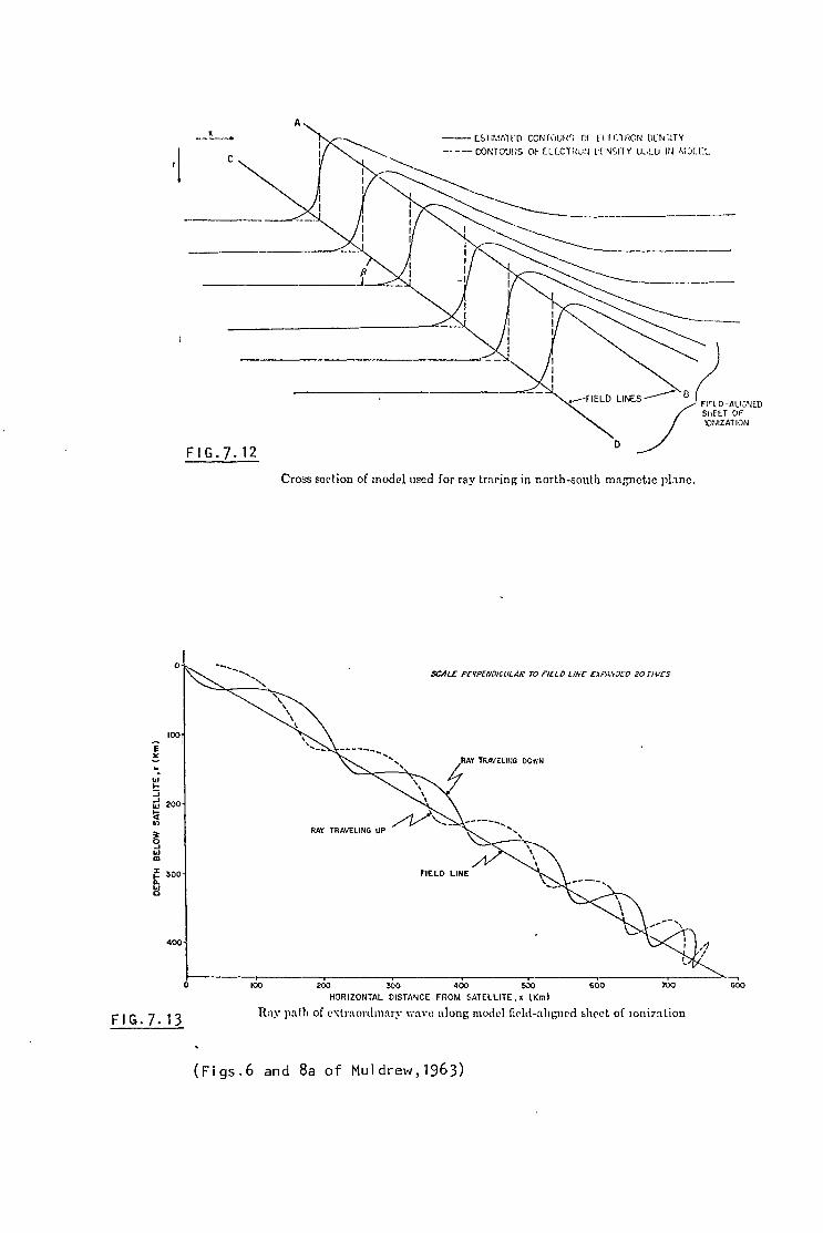
E ><
w ._ :;
0
100 I
.i 200
Ii ., ~ w m
~ 300 ... "' 0
400
FIG.7.13
--- £.S rn.\t.1 rn CONTlJUW; r:r rt fr, rnoN on<.:TY
-- ---CONlOUfiS o~ [LlCmc:~J l'l N'OITY u~L[J Ill MXl:L c
~ .-FIELD LINES___.. !l
FIG.7.12 D
Cross scrtion of model used for ray traring in north-south nrngnct1e plane.
SCALE PHPEllCl!CIJlAR TO FIELD LINC C>f'A.\OEO 20 TIVCS
0 100 200 300 400 5.:xJ 600 700
HORIZONTAL DISTA'lCE FROM SATELLITE, 1 !Km)
Ray p:tt!1 of c'\lraonl11rnry Y•nve along model fiP!d.-nhr;ncd ~hcct of 1011i7nlion
(Figs.6 and Sa of Muldrew, 1963)
F:rLD-ALl-3t-~t..D
Sl1EET OF IOWZATl0N
000
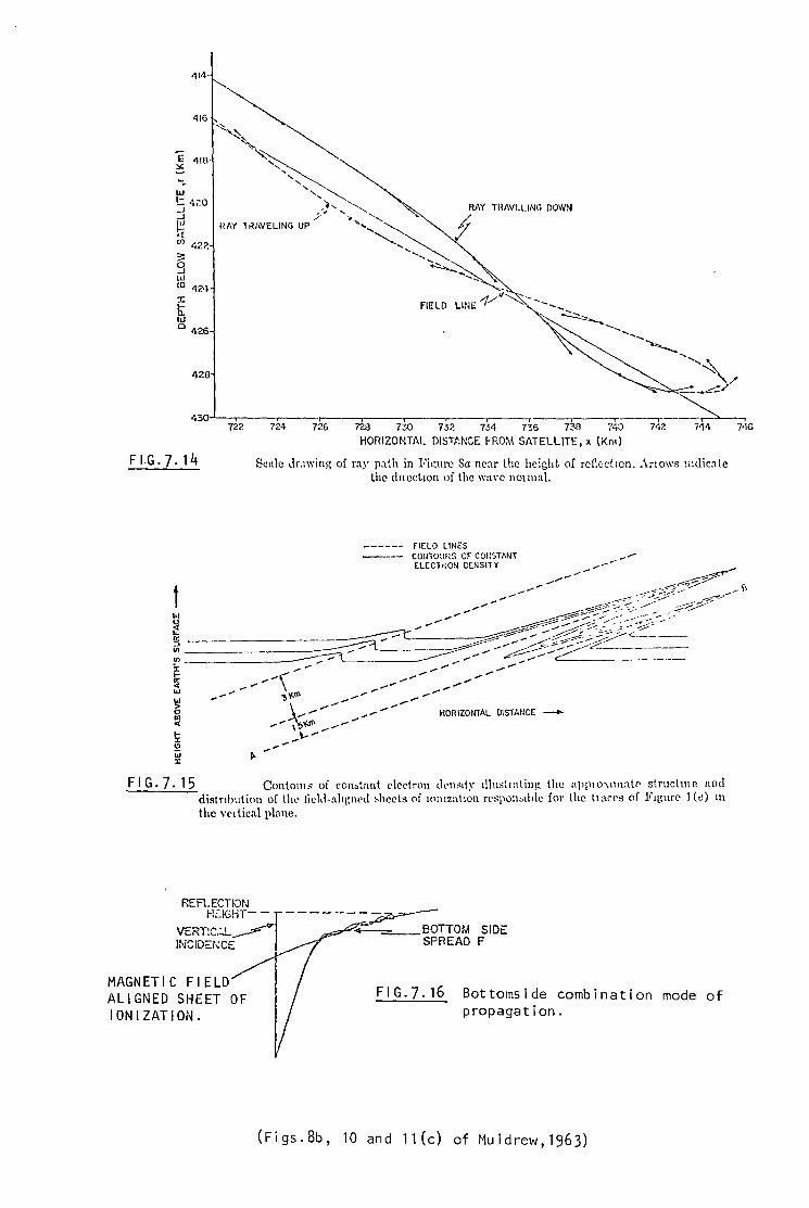
414
416
'E 4m :.::
428
-~
' ' '" ',,~
,~ .... "" RllY TRl\VLl.ING DOWN
/ ...... "· .::-~.... . "". / l!f1Y l~/IVELING UP ~ ................... ~ /.f
............ ~--~ "-~
FIELD LINE-'//"~-----~ ..... _
----~ ..... ............ ~/ ~~/
430,-'---~--~-- ~-----------------,-----,--.-----,--~ 722 724 726 728 730 732 734 BG 7~ "ft.0 ·142 7'14 ""16
HORIZOMTAL DJSTf,NCE FROM SATELLITE, x {Km)
Fl.G.7.14 Scale ,\r.nring of ray p.1th in 1-'kurc Sa nc:lr the height of rc!lc:ct1on .• \nows mtlic:lle the d11ect10n of the w:n-c nounal.
flELO LINES COIHOURS OF COl~ST/\NT ELECl tWN DENSITY ... ,....--
FIG· 7. 15 Contoms of con~trmt electron d,·n~1ty 11lust1:1lin~ the ap]liO"\tmalP structu1c nnd distribution of th,• tiehl-:1l1t:1wd ~111~cl:1 oi wn1z:1l1on rcspon~1!.le for the l1a~P:1 of F1!.'urc 1 (c) m the w1 lieal plane.
REFLECTION H.C:IGHT- -
VERTlC.:.L~ INCIDEr.:CE
MAGNETIC FIELD ALIGNED SHEET OF IONIZATION.
(Figs.Sb,
FIG.7.16 Bottomside combination mode of propagation.
10 and 11 (c) of Muldrew, 1963)
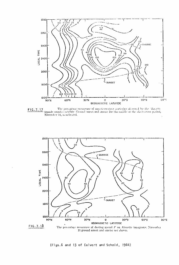
)) ~ --
x~~L _____ 0
I __L..!:J_L 30'N , 'ETIC LATITUD< ,. ii•• """"'"
12
00 -'- 60'N GEO>,AG<. • , ,. "'•·'"'"''' 1,_, . '"n j)1_1iod, 90'N ,, '"," '" ' , " < , '"' .,,,.
__ , __ .J _______ ·--;O"'; l --- coos
'lf' l Lil~ L '-l'I \.ti ·1·1tl'l' of as11,·,·L- c n, for tlic mid" ' " . nl :11~l' o< i·u11 •l an• I .olllll l>-1 'J'J11• J•l'l'.l f:101111•l ~llB'l 7 id· I >-alr·lhlr FIG. 7 · 1 tops1dC' ''.rn~. 1 • 1 ,, 111<11r.dr-d.
Ill
""
Nm·r111l· 1 r
t= NO -J <t 0 0 --'
FIG.7.1B
(Figs.6 and 13 o "d 1964) and Schm1 ' f Calvert
90°S
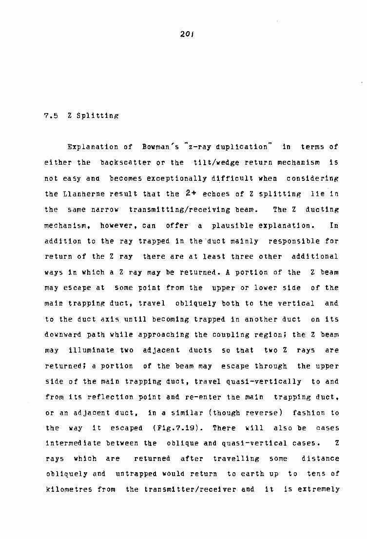
201
7.5 Z Splitting
Explanation of , " " Bowman s z-ray duplication in terms of
either the backscatter or the tilt/wedge return mechanism is
not easy and becomes exceptionally difficult when considering
the Llanherne result that the 2+ echoes of Z splitting lie in
the same narrow transmitting/receiving beam. The Z ducting
mechanism, however, can offer a plausible explanation. In
addition to the ray trapped in the-duct mainly responsible for
return of the Z ray there are at least three other additional
ways in which a Z ray may be returned. A portion of the Z beam
may escape at some point from the upper or lower side of the
main trapping duct, travel obliquely both to the vertical and
to the duct axi~ until becoming trapped in another duct on its
downward path while approaching the cou~ling region; the Z beam
may illuminate two adjacent ducts so tnat two Z rays are
returned; a portion of the beam may escape through the upper
side of the main trapping duct, travel quasi-vertically to and
from its reflection point and re-enter tne main trapping duct,
or an adjacent duct, in a similar (though reverse) fashion to
the way it escaped (Fig.7.19). There ~ill also be cases
intermediate between the oblique and quasi-vertical cases. Z
rays which are returned after travelling some distance
obliquely and untrapped would return to earth up to tens of
kilometres from the transmitter/receiver and it is extremely
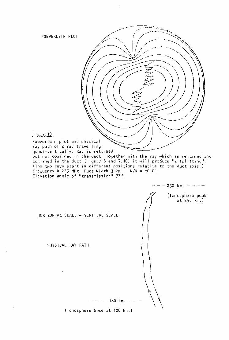
POEVERLE IN PLOT
FIG.7.19
Poeverlein plot and physical ray path of Z ray travelling quasi-vertically. Ray is returned but not confined in the duct. Together with the ray which is returned and confined in the duct (Figs.7.6 and 7.10) it will produce "Z splitting". (The two rays start in different positions relative to the duct axis.) Frequency 4.225 MHz. Duct Width 3 km. N/N = ±0.01. Elevation angle of "transmission" 72°.
HORIZONTAL SCALE VERTICAL SCALE
PHYSICAL RAY PATH
----180km.---
(Ionosphere base at 100 km.)
- - - 2 30 km. - - - -
\ \
(Ionosphere peak at 250 km.)
unlikely that detection would take place in the majority of
these cases. Z rays which illuminated two ducts would both be
detected. The degree of frequency separation of the two echoes
would depend upon both the relative strengths of the ducts and
also on the N-S horizontal gradient. In tne case of the Z ray
travelling quasi-vertically the frequency separation will again
depend on both the duct strengths and the N-S horizontal
gradient but in this case the horizontal gradient will be more
important owing to the separation of the reflection points of
the trapped and vertical Z rays. Muldrew's (1963) model fitted
to an actual topside record (Fig.?.15) is an example of ducts
which; if both illuminated by the Z beam, would produce Z
Splitting. The so called ., ., diffuse Z echo observed by Bowman
on 16% of the September 1946 Hobart records ~e examined is
probably a variation of the splitting situation where the
frequency separation between traces is very small.
7.6 Discussion
The ray tracing model of the duct theory was unable to
establish trapping criteria although it did establish that
trapping could take place. We may, however, speculate on
trapping criteria with qualified assistance from those results
which were obtained from the models.
The trapped ray must travel through two different trapping
regions on its path from the coupling point to the reflection
point and back down to the coupling point. The boundary of
these regions may be taken on the Poeverlein diagram as the
contour where the curves change from concave only to concave
and convex as viewed from the centre point of the diagram.
These regions will be referred to as the upper (or inner) and
lower (or outer) trapping regions (Fig.7.1). On leaving the
vicinity of the coupling point on the Poeverlein diagram the
ray path on the Poeverlein diagram follows the direction of
-grad.N. If the duct is too weak to trap the Z ray (the
ionization contours are not sufficiently perturbed as to become
perpendicular to the duct axis) then the path followed will be
similar to that for a ductless ionosphere except that the
straight line path will be rippled as the ray crosses
successive ducts. If the duct is sufficiently strong to have
ionization contours perpendicular to the magnetic field line
(duct axis) but sufficiently weak that the contours do not
deviate far from perpendicularity to the axis over a reasonable
part of the duct width then trapping will be easily
accomplished by the lower trapping region. A stronger duct
will have less of its cross section nearly ~erpendicular to the
duct axis and less of the duct will be available for easy
trapping in the lower region. Furtnermore, the ray may more
quickly stray to less favourable contours so that the wave
normal is at too great an angle for trapping when entering the
upper reRion. Under these circumstances, an increase in tbe
width of the duct will clearly increase trapping efficiency.
20S'
If the duct is very strong the Poeverlein ray path will
approach perpendicularity to the field direction and the ray
path may reach the concave section of the lower region curves
without leaving the duct (such a path on this part of the
Poeverlein diagram would be in a direction of slow increase of
electron density which would facilitate reaching the desired
part of the diagram while remaining in the duct) and trapping
may again occur. In the upper trapping region trapping is much
simpler: the steeper the duct sides, the easier the trap~ing
(in that rays having larger wave normal angles with tne axis
may be trapped. Also the steeper the sides in the upper
trapping region the more likely the trace will pass through the
centre of the Poeverlein diagram or a point near tne
the diagram so that the ray may trace a path to
coupling point).
centre of
the lower
The shape of the duct is determined
electron density deviation from ambient
ionospheric electron density gradient.
by its width, its
and the vertical
If the first two
parameters remain fixed throughout the duct tnen the shape of a
particular electron density contour depends upon the vertical
gradient at that level. For situations other than very strong
ducts we ~refer the duct to be shallow walled in the lower
trapping region and steeper walled in the u~per trapping
region. ~here is a part of the ionosphere which provides these
conditions very well: that is tne ~art of the ionosphere below
the peak where the vertical electron density gradient weakens
rapidly with neight. If the coupling point is at an altitude
where the vertical gradient is still steep but not far below
where it begins its rapid decrease then in the lower coupli~g
re~ion the duct may be shallow sided with tne sides becoming
steeper as we progress upwards and into the up~er coupling
region. Strong duct trapping will also be assisted at
altitudes near the layer peak as the duct sides will be steeper
here. If our speculation is correct then the Z echo should
often be seen on the critical part of its trace. This turns
out to be the case for original records, although it is not
necessarily so true of published Z echoes (authors have
probably selected strong examples of the Z echo in ' preference
to typical examples). As already noted in Section 3.3,
Ellis (1954) found that there was an increase in the Z echo
amplitude near the critical frequency on all four occasions on
which he recorded the variation of echo amplitude with
frequency. His results are shown in Fig.7.20. Ellis also
noted that It is characteristic of many P'f records of triple
splitting that the Z trace appears strongest near the Z
critical frequency". We futher note that two of Ellis's four
observations show a second increase in amplitude at a slightly
lower frequency. This may be seen on many n'f records as
several maxima (e.~.Fi~s.3.16, 3.44, 5.24 to 5.26) and the Z
trace sometimes takes on a "string of sausages'' appearance.
A~ain this is easy to explain in a ducting ionosphere. As the
frequency changes, so do the critical incidence angle and the
spatial coordinates of the coupling point. As the position of
201
the coupling point moves so may vary the trapping efficiency
and witn sufficient frequency change the coupling point may
progress into an adjacent duct. The form of the amplitude
peaks of the Z trace may reflect the structure of the ducts.
Trapping efficiency in a given duct may also vary with
frequency.
With regard to the physical path of the ray it can be seen
from the Poeverlein diagram that except in the immediate
vicinity of the coupling point the ray must stray well away
from the axis (throu~h the coupling points) of the diagram
before the group directions deviate significantly from the
magnetic field direction. Thus there would normally be no
problem with the ray moving rapidly from a favourable to an
unfavourable trapping environment.
Although spread-F correlates well with Z echoes on a
seasonal and sunspot cycle variation there is not a diurnal
correlation. In the case of Hobart the Z mode is predominantly
a daytime phenomenon and is usually associated only with
spreading which is weak. The major diurnal occurence of Z echo
at Hobart occurs early in the daylight sector when spread-F
(which has been evident during the night) is disappearing. It
may be that the strong spread-F at night is associated with
moderately strong ducts not favourable to Z ray trapping in the
lower trapping reRion. The weuKel'JlilJ of these ducts around dawn
may facilitate Z ray trapping whilst producing only weak or
---------
208
barely detectable spreading. It should be noted that Calvert
and Schmid (1964) found the highest percentage occurence of
ducting spread-F at latitudes roughly corresponding to those
found by Bowman (1960) to show the greatest occurrence of Z
echo (Figs.3.24 and 7.18). Examination of Fig.7.18 shows that
within the belt of ducting spread-F the occurrence at night is
greater than that in the daytime. However, if the nignt
occurrence also represents stronger ducts which find Z ray
trapping more difficult then the diurnal occurrence of Z echo
would not follow tne diurnal behaviour of Fig.7.18. ' '
If the
ducts responsible for strong spreading become sufficiently
strong for strong trapping in the lower trapping region then we
will have Z echoes on records snowing strong spreading and we
might expect these Z echoes on average to exhibit an increase
in echo amplitude and/or the spectral range of the Z echo. Z
echos in association with strong spreading are seen quite often
on Hobart night time records.
So far we nave seen that ducting is a possible Z return
mechanism and can fit tne available evidence quite well. I
Despite this, we have not yet shown that there is any direct
evidence of duct return of the Z ray. Fortunately there is a
paper in the available literature which provides such evidence
and we describe the experiment and results in the next section.
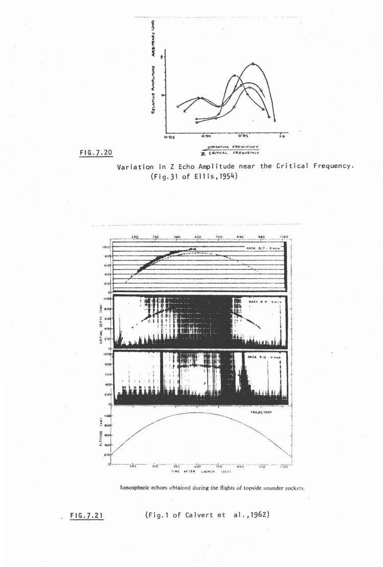
FIG.].20
-- --- ----
~ ... 1 ~ • t !
.. 0
~ l • f < " .. > ~ .. .. ct
O ·SS O ·')O 0 ·9S l·O
Of'C.tAT•r4f,. FA.f!:~UF""("'
~ C~1Tlt.At.. F~•QLJIFNt.V
Variation in Z Echo Amplitude near the Critical Frequency. (Fig.31 of Ellis,1954)
240 lOO 720 600_ 4'-0 tlO t080 -,----- -,-- -- -- ,.. -, •10
..... -----···-· t ~~~~~~~~~------.]
I - - - - - l..---· • ·- '-----& ---------·-·-·· L--... -'"o .. so eoo n o a•o itfl.O
flflif( ., f [lt LAUHC!i !St.C l
Ionospheric echoes obtained during the flights of topside sounder rockc s.
FIG.].21 (Fig. 1 of Calvert et al. ,1962)
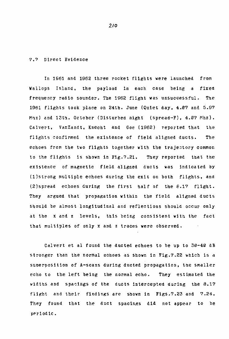
210
7.? Direct Evidence
In 1961 and 1962 three rocket flights were launched from
Wallops Island, the payload in each case being a fixed
frequency radio sounder. The 1962 flight was unsuccessful. The
1961 flights took place on 24th. June (Quiet day, 4.07 and 5.97
M~z) and 13tn. October (Disturbed night (spread-F), 4.07 Mhz).
Calvert, Vanzandt, Knecht and Goe (1962) reported that the
flights confirmed the existence of field aligned ducts. The
echoes from the two flights together with the traje~tory common
to the flights is shown in Fig.7.21. They reported that the
existence of magnetic field aligned ducts was indicated by
(l)strong multiple echoes during the exit on both flights, and
(2)spread ec~oes during the first half of the 8.17 flight.
They argued that propaRation within the field aligned ducts
should be almost longitudinal and reflections should occur only
at the x and z levels, this being consistent with the fact
that multiples of only x and z traces were observed.
Calvert et al found the ducted echoes to be up to 30-40 dB
stronger than the normal echoes as shown in Fig.7.22 which is a
superposition of A-scans during ducted propagation, the smaller
echo to the left being the normal echo. They estimated the
widths and spa~ings of the ducts intercepted during the 8.17
flight and their findings are shown in Figs.7.23 and 7.24.
They found that the duct spacin~s did not appear to be
pPriodic.
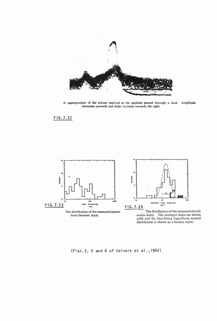
.ti . '\
A superposition of the echoes received as the payload passed through a duct. Amplitude increases upwards and delay increases towards the right.
FIG.7.22
..
.. " w . ~
FIG.7.23 1.0 ... ....
°"'' ICPU.\TIOtl .... The distribution of the measured separa
tions between ducts.
II
10 . w . i
0
OJ 1.0 .... APl'All:tlf\ DUct DIAWlTUt
FIG.].24 U•I
The distribut ion of the measured chords a..:ross ducts. The strongest ducts are shown solid and the best-fitting logarithmic nonnal distribution is shown as a broken curve.
(Figs.3, 5 and 6 of Calvert et al. ,1962)
212.
Singleton and Lynch (1962) found that the field aligned
irregularities occur in patches and there is other evidence
supporting this view. For instance, Calvert et al found Z
ducting over only half the rocket trajectory and not at the
lower latitudes. Given a paten of ducts with non periodic
spacing, we have an excellent model to simulate the detailed
occurrence patterns of the Z echo. As these ducts either
drift, or dissolve and reform at non periodic intervals; we
will have Z echoes which will appear and disappear in a non
periodic fashion. The z echoes will continue their
intermittent presence for time an indefinite period of
depending on how long the patch is in the vicinity of the
ionosonde. This may be a matter of minutes or hours. This is
exactly the observed behaviour of Z ecnoes (Figs.5.29 and
5. 30). NOTE ON POEVERLEIN PLOTS.
When (as is the case with the ionospheres described in this chapter) the
magnetoplasma is not plane stratified then the method of Poeverlein as
described in Section 2.4 may be no longer easily applied. Nevertheless, the principles expounded by Poeverle1n may be utilised and the Poeverlein diagram is now treated as a refractive index space where the locus of the refractive index vector along the path of the ray can be drawn and the outward normal to
a refractive index surface at its point of intersection with the locus gives the direction of the ray at the corresponding point in the medium. This
application of the Poeverlein diagram has previously been employed as an aid in interpretating magnetospheric and solar radio wave ray tracing and.is well
described by Herring (1980).
8.1 Summary
CHAPTER EIGHT
CONCLUSIONS
Two alternative mechanisms postulated for return of tne Z
ray have been examined and experiments carried out to
investigate which of the mechanisms is operating during the
presence of the Z echo. The results of the experiments taken
together with the results of previous experiments effectively
demonstrate that neither the backscattering mechanism nor the
tilt/wed~e mechanism is a suitable explanation of Z ray return
in the overwhelming majority of Z echo cases.
The duct mechanism of Z ray return has been proposed in an
endeavour to overcome some difficulties encountered with t~e
previous proposals. The duct mechanism is able to explain many
features of Z echoes not easily accounted for by the other
mechanisms; some ray tracing models have
the Z ray in a ducting ionosphere;
successfully returned
and in addition to
substantial circumstantial existing evidence favouring the duct
model there is a report of two rocket flight sounding
experiments which provides direct evidence of Z ducting at Z
echo latitudes (Wallops Island dip angle is 70°). The Z duct
model is the obvious choice of those mechanisms so far proposed
to account for return of the Z ray.
214-
8.2 Recommendations For Future Research
It is important that the criteria for trapping be
established. This will probably require modelling using
techniques such as full-wave analysis at least in the vicinity
of the coupling region. Workers who have already carried out
detailed modelling studies of the coupling region (e.g.
Smith,19?3; Budden,1980) may be ~ell equipped to carry out such
an investi~ation. Once trapping criteria are established it
may be possible to obtain a great deal of information about the
presence, type, structure and spacing of ducts from routine h'f
ionograrns. This in turn will assist spread-F (including
artificially created spread-F) and other duct related studies
and may have a bearing on the overall picture of
ionosphere/plasma sphere and ionosphere/magnetosphere ' interactions. For instance, there is some similarity between
the patterns of presence and strength (''fading .. patterns, for
want of a more appropriate term} of some micropulsations and
the z echo. Fraser-Smith (1981) recently reported on the
occurrence of mid-latitude Pc 1 and there is in his plot
(Fig.8.1} a sugRestion of an inverse sunspot cycle relationship
reminiscent of that found by Bowman (1960) for Z echo
occurrence. It should be pointed out that Fraser-Smith did not
find an eleven year periodicity in his data: nevertheless, tne
possibility of a link between Z ducts and micropulsations is
215
worth pursuing at this stage. There may also be a connection
between Z ducts and those of whistlers. Andrews (1975) found
similarities between whistler rates and the incidence of mid
latitude spread-F in both time and space for the years 1963 to
1968. He noted that other workers had also found an
association between whistler propagation and spread-F
occurrence. Singleton (1961) noted reports of the dependence
on geomagnetic latitude of whistler incidence. One worker
reported a maximum at about 45° geomagnetic latitude while
another group put the maximum whistler occurrence at 50°
geomagnetic latitude but both reported a marked decrease in
whistler activity at higher and lower latitudes. The latitude
belt of whistler activity is similar to tnat found by
Bowman (1960) for Z echo occurrence.
Z duct origins may possibly be found in the existing
explanations for, and postulates of, otner field aligned
phenomena. For instance, in the existing literature are such
suggestions as field aligned plasma interchange between
ionosphere and plasmasphere (e.g.Carpenter and Park,19?3;
Park,1973); and growth of field aligned irregularities from
ionospieric turbulence (e.g.Booker,1956). There have also been
suggestions that atmospheric gravity waves dissipate energy
through turbulence (e.g.Bretherton,1969} and so there may
possibly be an indirect connection between TID's and Z ducts.
It is noted that the presence of the Z echo is not
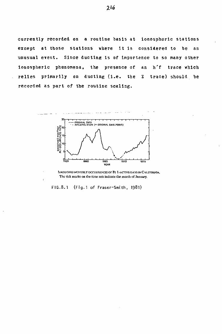
216
currently recorded on a routine basis at ionospheric stations
except at those stations where it is considered to be an
unusual event. Since ducting is of importance to so many other
ionospheric phenomena, the presence of an h'f trace which
relies primarily on ducting (i.e. the Z trace) should. be
recorded as part of the routine scaling.
-- - - .....--- - - ---- -- -- - - - -- - -- - -- - -
-- O::!IGINAL DATA · - INfERPOLATION (• ORIGINAL DATA POINT!
1955 1960 1965 YEAR
/ 1970 1975
~:-IOOTHED MmmtLY OCCURRF-'<CES OF Pc 1-ACTIVE DAYS IN Co.UFORNIA.
The tick marks on the time axis indicate the month of January.
FIG.8. 1 (Fig. 1 of Fraser-Smith, 1981)
2/7
SELECTED BIBLIOGRAPHY
ANDREWS,~.K.: 1975, J.Atmos.Terr.Phys. 37, 1423.
BANERJI,R.B.: 1S52, Ind.J.Phys. 26, 28.
BOOKER,H.G.: 1936, Proc.Roy.Soc. A155, 235.
BOOKER,H.G.: 1938, Phil.Trans.Roy.Soc. A237, 411.
BOOKER,H.G.: 1955, J.Atmos.Terr.Phys. 7, 343.
BOOKER,H.G.: 1956, J.Geophys.Res. 61, 673.
BOOKER,q.G.: 1961, J.Geophys.Res. 66, 1073.
BOWLES,K.L.: 1958, Phys.Rev.Letters 1, 454.
BOWMAN,G.G.: 1960, Planet.Space Sci. 2, 214.
BOWMAN,G.G.: 1960a, Planet.Space Sci. 2, 133.
BOWMAN,G.G.: 1960b, Planet.Space Sci. 2, 150.
BRITREBTON,F.P.: 1969, Radio Science 4, 1279.
BRIGGS ,B.F. and PHILLIPS,G.J.: 1950, Proc.Phys.Soc. 63B, 907.
BUDDEN,K.G.: 1961, "Radio Waves in the Ionosphere'', Cambridge Uni. Press, Cambridge.
BUDDEN,K.G.: 1964, "Lectures on Magnetoionic Theory'', Gordon and Breach, New York.
BUDDEN,K.G.: 1980, J.Atmos.Terr.Phys. 42, 287.
CALVERT,W.and COHEN,R.: 1961, J.Geopbys.Res. 66, 3125.
CALVERT,W. and SCHMID,C.W.: 1964, J.Geophys.Res. 69, 1839.
CARPENTER,D.L. and PARK,C.G.: 1973, Rev.Geophys.Space Phys. 11, 133.
DAVIES,K.: 1965, Ionospheric Radio Propagation", National ~ureau of Standards, Washington.
DIE~INGER,W. and MOLLER,F.G.: 1949, Die Naturwiss. 36, 56.
ECKFRSLEY,T.L.: 1933, Proc.Roy.Soc. A141, 710.
218
ECKERSLEY,T.L.: 1950, Proo.Phys.Soc. 63B, 49.
ELLIS,G.R.A.: 1953a, Nature 171, 258.
ELLIS,G.R.A.: 1953b, J.Atmos.Terr.Phys. 3, 263.
FLLIS,G.R.A.: 1954, "The Magneto-ionic Triple Splitting of Ionospheric Echoes", Ph.D. Thesis, University of Tasmania.
ELLIS,G.R.A.: 1956, J.Atmos.Terr.Pnys. 8, 43.
ELLIS,G.R.A.: 1957, J.Atmos.Terr.Phys. 11, 54.
ELLIS,G.R.A.: 1972, Proc.Astron.Soc.Aust. 2, 135.
FRASER-SMITH,A.C.: 1981, Planet.Space Sci. 29, 715.
HAJKOWICZ,L.A.: 1972, Can.Journ.Phys. 50, 2654.
HARANG,L.: 1936, Terr.Mag.Atmos.Elect. 41, 160.
HASELGROVE,J.: 1954, Rep.Conf.Phys.Ionosphere, p355, Phys. Soc.London, London.
BIBBERD,F.H.: 1971, J.Atmos.Terr.Phys. 33, 783.
HOGARTH,J.F.: 1951, Nature 167, 943.
JONES,R.M. and STEPHENSON,J.J.: 1975, "!Versatile Three Dimensional Ray Tracing Computer Program for Radio Waves in the Ionosphere", OT Report 75-76, Washington.
KLEMPERER,W.K.: 1963, J.Geophys.Res. 68, 3191.
LANDMARK,L.: 1952, J.Atmos.Terr.Phys. 2, 254.
LOCKWOOD,G.E.K.: 1962, Can.J.Pnys. 40, 1840.
LUI,C.H. and YEH,K.C.: 1977, J.Atmos.Terr.Phys. 39, 149.
MEIK,J.H.: 1948, Nature 161, 597.
MILLINGTON,G.: 1954, Proc.Inst.Elec.En~rs. 10l(Pt.4), 235.
MULDREW,D.B.: 1963, J.Geophys.Res. 68, 5355.
MULDREW,D.E.: 1980, J.Geophys.Res. 85, 613.
MUNRO,G.H.: 1950, Proc.Roy.Soc. A202, 208.
MUNRO,G.H.: 1953, Proc.Roy.Soc. A219, 447.
NEWSTEAD,G.: 1948, Nature lEl, 312.

21'1
PAPAGIANNIS,M.D.: 1965, J.Atmos.Terr.Pnys. 27, 1019.
PAPAGIANNIS,M.D.: 1972, "space Physics and Space Astronomy~, Gordon and Breach, London.
PAPAGIANNIS,M.D. and MILLER,D.L.: 1969, J.Atmos.Terr.Phys. 31, 155.
PARK,C.G.: 1973, J.Geophys.Res. 78, 672.
PITTEWAY,M.L.V.: 1958, Proc.Roy.Soc. A246, 556.
PITTEWAY,M.L.V.: 1959, Phil.Trans.Roy.Soc. !252, ~3.
PITTEWAY,M.L.V. ana COHEN,R.: 1961, J.Geophys.Res. 66, 3141.
POEVERLEIN,H: 1948, S.ber.Bayer.Akad., 175.
POEVERLEIN,H.: 1949, Z.angew.Phys 1, 517.
POEVERLEIN,H.: 1950, Z.angew.Phys. 2, 152.
RATCLIFFE,J.A.: 1962, "The Magneto-ionic Theory and its Applications to the Ionosphere", Camb.Uni.Press, London.
RATCLIFFE,J .A.: 1972, "An Introduction to the Ionosphere and Magnetosphere", Carob.Uni.Press, Cambridge.
RATCLIFFE,J.A. and WEEKES,K.: 1960, "Physics of the Upper Atmosphere", ed. J.A.Ratcliffe, Academic Press, New York.
R 'E:B ER , G • : 1956, J.Geophys.Res. el, 157.
PENAU,J.: 1959, J.Geophys.Res. 64, 971.
RENAU,J.: 1960' J.Geophys.Res. 65, 2269.
RI VA ULT, R. : 1950, Proc.Phys.Soc . 63B, 126.
RYDBECK,O.E.H.: 1950, J.Appl.Pnys. 21, 1205.
SATYANARAYANA,R., BAKRU,K. and KHASTGIR,S.R.: 1959, J.Atmos. Terr. Phys. 13, 201.
SCOTT,J.c.w.: 1950, J.Geophys.Res. 55, 65.
SCHMERLING,E.R.: 1958, J.Atmos.Terr.Phys. 12, 8.
SINGLETON,D.G.: 1961, Nature 189, 215.
S!NGLETON,D.G. and LYNCH,G.J.E.: 1962, J.Atmos.Terr.Pnys. 24, 3~3.
SINGLETON,D.G. and LYNCH,G.J.E.: 1962a, J.Atmos.Terr.Phys, 24, 3b3.
220
SMITH,M.S.: 1973, Nature Phys.Sci. 243, 29.
TAYLOR,~.: 1933, Proc.Phys.Soc. 45, 245.
TAYLOR,M.: 1934, Proc.Phys.Soc. 46, 408.
TOSHNI~AL,G.R.: 1935, Nature 135, 471.
YEH,K.C. and LUI,C.H.: 19?2, "Theory of Ionospheric Waves", Acade~ic Press, New York.
I ~ ADDITIONAL REFERENCES FOR CHAPTER SEVEN.
CALVERT, W.
HERRING, R.N.
LESTER, M. & A.J.SMITH.
STRANGEWAYS, H.J.
STRANGEWAYS, H.J. & RYCROFT M.J.
1981, J. GEOPHYS. RES. 86, 1609.
1980, J. ATMOS. TERR. PHYS. 42, 885.
1980, PLANET.SPACE SCI. 28, 645.
1981, J.ATMOS. TERR. PHYS. 43, 231.
1980, J.ATMOS. TERR, PHYS. 42, 983.