The investigation on SIMPLE and SIMPLER algorithm ... investigation on SIMPLE and SIMPLER algorithm through lid driven cavity Lee Chern Earn 1, Tey Wah Yen 1,2, ∗, Tan Lit Ken 2

Journal of Advanced Research in Fluid Mechanics and Thermal Sciences 29, Issue 1 (2017) 10-23

10

Journal of Advanced Research in Fluid

Mechanics and Thermal Sciences

Journal homepage: www.akademiabaru.com/arfmts.html

ISSN: 2289-7879

The investigation on SIMPLE and SIMPLER algorithm through

lid driven cavity

Lee Chern Earn1, Tey Wah Yen1,2,∗, Tan Lit Ken2

1 Department of Mechanical Engineering, Faculty of Engineering, UCSI University Kuala Lumpur, Malaysia 2 Malaysia-Japan International Institute of Technology (MJIIT), Universiti Teknologi Malaysia Kuala Lumpur, Malaysia

ARTICLE INFO ABSTRACT

Article history:

Received 9 January 2017

Received in revised form 6 February 2017

Accepted 7 February 2017

Available online 16 February 2017

The present study analyzes in details to compare SIMPLE and SIMPLER algorithm in

terms of their convergence rate, iteration number and computational time. The work

which is based on primitive variables (u, v, P) formulation of Navier-Stokes equations

to investigate the velocity and pressure distribution in the square cavity at Reynolds

number of 100 and 400. The solutions are obtained for grid size 16 × 16 up to 256 ×

256. From the plots of velocity profiles along centerline geometry, it shows good

agreement with the benchmark solution from past researchers. The velocity and

pressure in the cavity varies as the Reynolds number increases from 100 to 400.

SIMPLER algorithm is proven to be more efficient compared to SIMPLE as iteration

number required for a given Reynolds number and grid size is lower than that of

SIMPLE. The values of under-relaxation factors for velocity components and pressure

play significant role in terms of convergence rate of a numerical scheme.

Keywords:

SIMPLE algorithm, SIMPLER algorithm,

Lid driven cavity, Navier-Stokes

equations, Computational cost Copyright © 2017 PENERBIT AKADEMIA BARU - All rights reserved

1. Introduction

Lid driven cavity [1,2] is a classic benchmark problem for viscous incompressible flow [3-5]. The

model is able to exhibit various types of phenomena that can happen in an incompressible flow such

as secondary flows, transition to turbulence, eddy flows and complex three-dimensional patterns

[6,7]. In order to solve the incompressible Navier-Stokes equations, various methods have been

developed and the commonly used numerical procedure is Semi-Implicit Method for Pressure Linked

Equation (SIMPLE) and SIMPLER (SIMPLE – Revised) by [8].

Yapici and Uludag [9] have used finite volume method (FVM) of two-dimensional square lid driven

cavity flow at high Reynolds number (Re). The coupled flow equation is solved by SIMPLE algorithm.

Moreover, he has used QUICK scheme to approximate the convection terms in the flow equations.

In the findings, the accuracy of a numerical solution can be improved by using a smaller mesh in the

regions of high gradients than the mesh size of bulk flow.

∗Corresponding author.

E-mail address: [email protected] (W.Y. Tey)

Penerbit

Akademia Baru

Open

Access

Journal of Advanced Research in Fluid Mechanics and Thermal Sciences

Volume 29, Issue 1 (2017) 10-23

11

Penerbit

Akademia Baru

Jing Yang et al. [10] have presented a model for pool boiling called CAS model. The numerical

model is commonly used to measure the heat transfer in the industries application. SIMPLER

algorithm is integrated with a cellular automata technique to investigate the pressure and

temperature during the boiling process as the cellular automata technique alone is not effective to

investigate the boiling process. From the results shown, the integration of the technique into the

algorithm has proven to be a good approach in obtaining data coherent with the benchmark solution.

Yin and Chow [11] have computed comparison of four algorithms in simulating atrium fire. The

four algorithms for solving the velocity-pressure coupled equations are SIMPLE, SIMPLER, SIMPLEC

and PISO. The numerical schemes are each tested with the relaxation factors. In the results, all four

algorithms provide similar data for the flow variables except for pressure. It is concluded in the

studies that SIMPLER is the viable algorithms used to solve the equations in simulating atrium fire.

Although SIMPLE and SIMPLER method is widely used to solve velocity-pressure coupling fluid

problems, the numerical comparison between them is still unclear. Hence, the objective of the

present study is to compare SIMPLE and SIMPLER in terms of convergence, iteration number and

computational time.

2. Numerical details

2.1. The governing equations

The incompressible two-dimensional Navier-Stokes equations can be written as follows:

�(�� + ��

�� + �� ) = − �

�� + �∇�� (1)

�(�� + ��

� + �� ) = − �

� + �∇�� (2)

�� + ��

� = 0 (3)

with ∇= � �� + � �

�. Expanding the terms on x- and y-momentum equations results in:

�(�� + ��

�� + �� ) = − �

�� + �(�� + ��

��) (4)

�(�� + ��

� + �� ) = − �

� + �(�� + ��

��) (5)

Based on Eq.s (3) – (5), a general transport equation can be written as follows:

�� (�∅) + �

�� (��∅) + �� (��∅) = �

�� Γ �∅�� + �

� �Γ �∅�� + �∅ (6)

where∅ is the dependent variable such as velocity, temperature and enthalpy, Γ is the diffusion

coefficient and �∅ represent the source term. The first term on LHS is the unsteady term and the

second and third term on LHS is the convection terms. Consider only the x-momentum equation, the

∅ in Eq. 6 is replaced by u-velocity. Using discretization method by staggered grid as explained in

detail by [4,10], discretized x-momentum equation is as follows:


Volume 29, Issue 1 (2017) 10-23

12

Penerbit

Akademia Baru

� � = �� + �� + �� + � � + !� = ∑ �#$�#$ + !�#$ (7)

where the coefficient ��, ��, ��, � are the convection – diffusion at the neighboring cell faces and

!� = (%& − %') + �&∆)∆*.

2.2. SIMPLE algorithm

The Semi-Implicit Method for Pressure-Linked Equations (SIMPLE) is originally proposed by [8].

The principle of SIMPLE is to create discrete pressure equation based on discrete continuity equation.

The u-momentum equation for control volume centred at e is given as:

�&�& = ∑ �#$�#$ + +&(, − ,�) + !&#$ (8)

A guessed pressure field denoted as P* is to replace onto the Eq. 8 to obtain guessed velocity

components of u* and v*:

�&�&∗ = ∑ �#$�#$∗ + +&(, ∗ − ,�∗) + !&#$ (9)

However, the guessed velocity components would not able to satisfy conservation of mass, in that

case, velocity and pressure are corrected by adding correction values:

� = �∗ + �.

, = ,∗ + ,. (10)

� = �∗ + �.

Relating Eq.s 8 - 10 gives:

�&�&. = ∑ �#$�#$. + +&(, . − ,�. )#$ (11)

The neighbouring values in Eq. 11 are omitted for approximation as the terms will not affect the

final solution due to the correction values, u’ will be zero when the solution converged. Then,

relating to Eq. 10 becomes:

�& = �&∗ + /&(, . − ,�. ) (12)

At this point, Eq. 12 is needed to satisfy the discretized continuity equation (��+)& − (��+)' +(��+)# − (��+)0 = 0, hence it is substitute into the continuity equation. The same goes for uw, un,

us which gives:

[(�/+)& + (�/+)' + (�/+)# + (�/+)#2, . = (�/+)&,�. + (�/+)',�. + (�/+)#,�. + (�/+)0, . +[(��∗+)' − (��∗+)& + (��∗+)0 − (��∗+)#2 = 0 (13)

Simplifying Eq. 13 leads to:

� , . = ��,�. + ��,�. + ��,�. + � , . + ! . (14)

where,


Volume 29, Issue 1 (2017) 10-23

13

Penerbit

Akademia Baru

�� = (�/+)&

�' = (�/+)'

�� = (�/+)#

� = (�/+)0

� = 4 �#$#$

! . = (��∗+)' − (��∗+)& + (��∗+)0 − (��∗+)#

Eq. 14 is a pressure correction equation, the momentum source term b’ is the mass imbalance

due to incorrect velocity field. When the source term reaches zero, it means that the solution has

converge.

2.3. SIMPLER algorithm

SIMPLER is a revised version of SIMPLE in which discretized continuity equation is used to derived

discretized equation for pressure instead of pressure correction equation. Pseudo-velocities are

introduced in SIMPLER, which can be defined as follows:

�5& = ∑ 678�7878 9$:6:

(15)

Substitute Eq. 15 into Eq. 8 gives:

�& = �5& + /&(% − %�) (16)

Substitute Eq. 16 into discretized continuity equation and rearranging the terms produces:

[(�/+)& + (�/+)' + (�/+)# + (�/+)#2% . = (�/+)&%� + (�/+)'%� + (�/+)#%� +(�/+)0% + [(��5+)' − (��5+)& + (��5+)0 − (��5+)#2 (17)

Eq. 17 can be further simplified into:

� % = ��%� + ��%� + ��%� + � % + ! (18)

where

�� = (�/+)&

�' = (�/+)'

�� = (�/+)#

� = (�/+)0

� = 4 �#$#$

! . = (��5+)' − (��5+)& + (��5+)0 − (��5+)#

After obtaining the pressure value, the following sequence is the same as SIMPLE in which the

pressure value is used to solve the discretized momentum equation.


Volume 29, Issue 1 (2017) 10-23

14

Penerbit

Akademia Baru

3. Results and discussion

3.1. Mesh independence study and validation

Prior to comparative study on computational efficiency of SIMPLE and SIMPLER model, the

validation is done by comparing the computed velocity value with the work of [13].

Extrema of velocity along geometry centreline at Re = 100 and Re = 400 are tabulated in Table 1

and Table 2. It is shown that both algorithms are able to produce results that are good agreement

with Ghia’s benchmark solution [13] as the grid increases. It can be said that grid independence is

achieved in this case.

For SIMPLE algorithm, the Navier-Stokes equations can only be solved up to 128 × 128 grid due

to the under-relaxation factors. Optimal value of relaxation factors could not be obtained, hence, the

solution oscillates and diverge at one point of the iteration. In the present study, convergence

criterion is set as 10-3 at which the simulation is terminated and assumed to reach steady state. The

convergence criterion defined in the present study is the summation of error of velocity components

and pressure,

; = ∑<∅#9= − ∅# < ≤ 10@A (19)

where ∅ represents primitive variables, n is the iteration step.

Table 1

Extrema of velocity along geometry centerline at Re = 100

Reference Grid umin vmax vmin

SIMPLE 16 × 16 -0.18011 0.14960 -0.20606

SIMPLER 16 × 16 -0.18741 0.16002 -0.23098

SIMPLE 32 × 32 -0.20687 0.17349 -0.24592

SIMPLER 32 × 32 -0.20555 0.17387 -0.24588

SIMPLE 64 × 64 -0.21265 0.17834 -0.25247

SIMPLER 64 × 64 -0.21183 0.17810 -0.25167

SIMPLE 128 × 128 -0.21373 0.17932 -0.25356

SIMPLER 128 × 128 -0.21349 0.17924 -0.25335

SIMPLER 256 × 256 -0.21391 0.17950 -0.25371

Ghia et al. [13] 129 × 129 -0.21090 0.17527 -0.24533

Table 2

Extrema of velocity along geometry centerline at Re = 400


SIMPLE 16 × 16 -0.17234 0.16559 -0.28274

SIMPLER 16 ×16 -0.17200 0.16585 -0.28220

SIMPLE 32 × 32 -0.24566 0.23069 -0.36796

SIMPLER 32 × 32 -0.24533 0.23085 -0.36778

SIMPLE 64 × 64 -0.29837 0.27849 -0.42560

SIMPLER 64 × 64 -0.29770 0.27749 -0.42458

SIMPLE 128 × 128 -0.31973 0.29701 -0.44629

SIMPLER 128 × 128 -0.31928 0.29602 -0.44564

SIMPLER 256 × 256 -0.32613 0.30172 -0.45178

Ghia et al. [13] 129 × 129 -0.32726 0.30203 -0.44993


Volume 29, Issue 1 (2017) 10-23

15

Penerbit

Akademia Baru

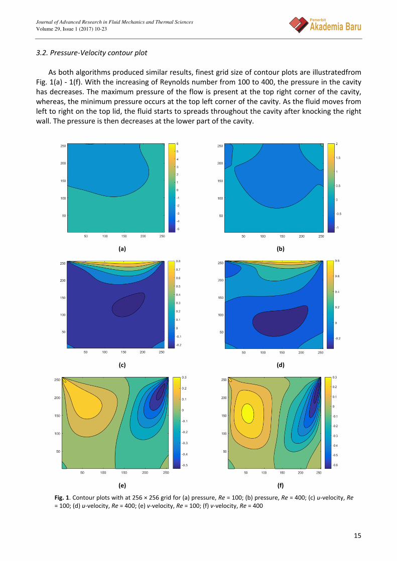
3.2. Pressure-Velocity contour plot

As both algorithms produced similar results, finest grid size of contour plots are illustratedfrom

Fig. 1(a) - 1(f). With the increasing of Reynolds number from 100 to 400, the pressure in the cavity

has decreases. The maximum pressure of the flow is present at the top right corner of the cavity,

whereas, the minimum pressure occurs at the top left corner of the cavity. As the fluid moves from

left to right on the top lid, the fluid starts to spreads throughout the cavity after knocking the right

wall. The pressure is then decreases at the lower part of the cavity.

(a) (b)

(c) (d)

(e) (f)

Fig. 1. Contour plots with at 256 × 256 grid for (a) pressure, Re = 100; (b) pressure, Re = 400; (c) u-velocity, Re

= 100; (d) u-velocity, Re = 400; (e) v-velocity, Re = 100; (f) v-velocity, Re = 400


Volume 29, Issue 1 (2017) 10-23

16

Penerbit

Akademia Baru

In the u-velocity contour plot, the velocity flow is dominant at the top lid due to stationary walls

on both sides. In addition to that, it can be seen that the boundary layer of the flow near the top

moving lid is thinner as the Reynolds number increases. The region of the minimum velocity has

increases and shifted towards the center of the cavity.

Due to the increase of Reynolds number, the velocity components have a higher magnitude

throughout the region inside the cavity. The bottom left and right corner of low velocity has covers

larger region as compared to at Re = 100. In v-velocity contour, the fluid flow is dominant on the left

wall and the flow is reverse on the right wall. At higher Re, the maximum and minimum v-velocity

regions spreads out, covers larger area in the cavity.

3.3. Velocity profile analysis

From Fig. 2 - 5, it is shown that the u-velocity and v-velocity profile along vertical and horizontal

centerline of geometry of cavity respectively are coherent with Ghia’s benchmark solution as the grid

size increases. However, SIMPLE algorithm unable to be implemented for 256 × 256 grid size due to

incompatible relaxation factors. Optimum relaxation factors for velocity and pressure cannot be

found, hence, cause the solution to oscillates and diverge.

The minimum u-velocity along the vertical centerline of the cavity and v-velocity at minimum and

maximum along horizontal centerline for various grid sizes are computed in Table 3. The minimum

u-velocity is denoted as umin and minimum and maximum v-velocity are denoted as vmin and vmax

respectively. As can be seen from the table, the extrema of velocity of grid size 128 × 128 and 256 ×

256 of SIMPLER algorithm does not differ much. This in turns shows that, the numerical solution will

no longer changes with the increasing of grid size, in other words, grid independence. Furthermore,

both SIMPLE and SIMPLER algorithms have implemented and converge to similar results.

Table 3

Extrema of velocity along the centerline of the cavity, Re = 100


SIMPLE 16 × 16 -0.18011 0.14960 -0.20606

SIMPLER 16 ×16 -0.18741 0.16002 -0.23098

SIMPLE 32 × 32 -0.20687 0.17349 -0.24592

SIMPLER 32 × 32 -0.20555 0.17387 -0.24588

SIMPLE 64 × 64 -0.21265 0.17834 -0.25247

SIMPLER 64 × 64 -0.21183 0.17810 -0.25167

SIMPLE 128 × 128 -0.21373 0.17932 -0.25356

SIMPLER 128 × 128 -0.21349 0.17924 -0.25335

SIMPLER 256 × 256 -0.21391 0.17950 -0.25371

Ghia et. al [10] 129 × 129 -0.21090 0.17527 -0.24533

In the simulation runs at Re = 400, the results obtained are also coherent with the benchmark

solution as shown in Fig.s 6 - 9. Both algorithms are implemented and matches well with Ghia as

the size of the grid increases. SIMPLE algorithm can only be implemented to solve up until 128 ×

128 due to incompatible relaxation parameters found.

As previously mentioned in the results at Re = 100, there is not much difference in extrema

velocity of grid size 128 × 128 and 256 × 256. However, at Re = 400, the velocity between the two

grid sizes has larger difference values as compared to the solution at Re = 100. It can be said that for

larger Reynolds number, finer grid size is required in order to reach grid independence. Similarly,

both SIMPLE and SIMPLER algorithm implemented is able to converge to the same extrema velocity

profiles at all grid sizes. This can be shown through Table 4.


Volume 29, Issue 1 (2017) 10-23

17

Penerbit

Akademia Baru

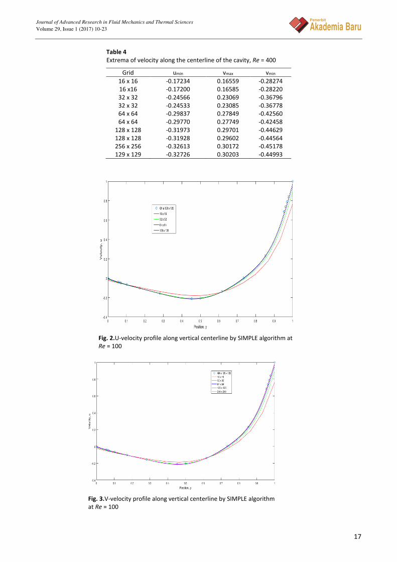
Table 4

Extrema of velocity along the centerline of the cavity, Re = 400

Grid umin vmax vmin

16 x 16 -0.17234 0.16559 -0.28274

16 x16 -0.17200 0.16585 -0.28220

32 x 32 -0.24566 0.23069 -0.36796

32 x 32 -0.24533 0.23085 -0.36778

64 x 64 -0.29837 0.27849 -0.42560

64 x 64 -0.29770 0.27749 -0.42458

128 x 128 -0.31973 0.29701 -0.44629

128 x 128 -0.31928 0.29602 -0.44564

256 x 256 -0.32613 0.30172 -0.45178

129 x 129 -0.32726 0.30203 -0.44993

Fig. 2.U-velocity profile along vertical centerline by SIMPLE algorithm at

Re = 100

Fig. 3.V-velocity profile along vertical centerline by SIMPLE algorithm

at Re = 100


Volume 29, Issue 1 (2017) 10-23

18

Penerbit

Akademia Baru

Fig. 4.U-velocity profile along horizontal centerline by SIMPLE algorithm at Re

= 100

Fig. 5.V-velocity profile along horizontal centerline by SIMPLE algorithm at

Re = 100

3.4. Computational Cost Study

The numerical solution is obtained on PC with Intel® Core™i5 processor and 8GB RAM. In general,

it can be seen that the iteration number and computational time to implement SIMPLE is much larger

than SIMPLER. For Re = 400 and at grid size 128 × 128, the iteration number and computational time

has reach as high as 127999 and 16228.38 seconds. Whereas, for SIMPLER algorithm, it can go as fast

as 1.03 seconds and only require 309 iterations to obtain the solution.

However, there is a set of values which does not follow the trend, at which at Re = 100 of grid

size 128 × 128, the iteration number and computational time required for SIMPLER is larger than that

of SIMPLE. The reason of this discrepancy is due to the relaxation factor used in the SIMPLE algorithm.

As mentioned in Chapter III, the algorithm is largely dependent on the relaxation factors. For this


Volume 29, Issue 1 (2017) 10-23

19

Penerbit

Akademia Baru

case, the relaxation factor selected could be the optimum value for the algorithm to run at that given

Reynolds number and grid size. The iteration number and computational time for SIMPLE algorithm

can be improved if an optimum relaxation factor can be found.

Fig. 6.U-velocity profile along vertical centerline by SIMPLE algorithm at Re =

400

Fig. 7.V-velocity profile along vertical centerline by SIMPLE algorithm at Re =

400

The convergence rate between SIMPLE and SIMPLER algorithms are compared and computed in

the Table 5 - 7. Referring to [14], the rate of convergence canbecalculated with the formula given as

follows:

BCD�EFGEDBEF�HE � log�<�LM7N�ON�@�LM7

P�QOP�Q<

<�LM7RSORS@�LM7

P�QOP�Q< (19)


Volume 29, Issue 1 (2017) 10-23

20

Penerbit

Akademia Baru

Fig. 8. U-velocity profile along horizontal centerline by SIMPLE algorithm at

Re = 400

Fig. 9.V-velocity profile along horizontal centerline by SIMPLE algorithm at

Re = 400

Grid size 128 O 128 is chosen as the reference solution. The ratio of the two errors can get an

estimate of the convergence. umin and vminof grid size 32 O 32, 64 O 64 and 128 O 128 at Re = 100

and Re = 400 are select from Table 1 – 2. Rateu and Ratevare the convergence rate for the umin and

vmin respectively. In the table, it shows that SIMPLER algorithm implemented at Re = 100 and Re =

400 has better convergence rate as compared to SIMPLE algorithm due to the smaller ratio in error.


Volume 29, Issue 1 (2017) 10-23

21

Penerbit

Akademia Baru

Table 5

Iteration number and computational time at Re = 100

Re = 100 Grid Iteration Number Computational Time (s)

SIMPLE 16 × 16 7039 17.17

SIMPLER 16 × 16 309 1.03

SIMPLE 32 × 32 11974 85.87

SIMPLER 32 × 32 1175 12.26

SIMPLE 64 × 64 13922 305.51

SIMPLER 64 × 64 4576 146.94

SIMPLE 128 × 128 17296 1244.98

SIMPLER 128 × 128 18169 2038.38

Table 6

Iteration number and computational time at Re = 400

Re = 400 Grid Iteration Number Computational Time (s)

SIMPLE 16 × 16 2745 9.40

SIMPLER 16 × 16 437 1.12

SIMPLE 32 × 32 8366 94.54

SIMPLER 32 × 32 1321 11.94

SIMPLE 64 × 64 21069 753.22

SIMPLER 64 × 64 3840 129.86

SIMPLE 128 × 128 127999 16228.38

SIMPLER 128 × 128 13705 1542.31

Table 7

Convergence rate at Re = 100 and Re = 400

Reference Reynolds

Number Rateu Ratev

SIMPLE 100 2.667 2.809

SIMPLER 100 2.258 2.153

SIMPLE 400 1.794 1.921

SIMPLER 400 1.777 1.886

4.Conclusion

In the present work, SIMPLE and SIMPLER are employed to investigate the pressure and velocity

distribution in lid driven cavity. Comparison have made between the two algorithms in terms of

convergence, iteration number and computational time. Numerical solution for the incompressible

flow at Re = 100 and Re = 400 up to 256 × 256 grid are computed. The results obtained compared

well with the benchmark solution from previous literature. The pressure and velocity distribution

changes according to the Reynolds number. The magnitude of the pressure and the location of the

minimum u-velocity region are affected by the variation of Reynolds number. From this study, it is

found that SIMPLER require less iteration number and computational time to converge solution

despite the extra computational load. The findings from this study are able to be used as a reference

by future researchers in the comparison of these numerical schemes.

Future improvement can be made on this study to improve the computational time of the

numerical schemes. FORTRAN can be used as it is better as compared to MATLAB with its

recognizable computational efficiency. This in turns improve the performance and encourages more

findings at higher Reynolds number and finer grid size in shorter amount of time. In addition, an

application of improvised under-relaxation method on SIMPLE algorithm can improve the

convergence rate and computational time. In this way, more results can be obtained if optimal


Volume 29, Issue 1 (2017) 10-23

22

Penerbit

Akademia Baru

relaxation factors are used in the numerical scheme. The solution will no longer oscillates heavily or

diverge.

Acknowledgement

The work is supported by Centre of Excellence for Research, Value Innovation and Entrepreneurship

(CERVIE) UCSI University under University Pioneer Scientist Incentive Fund (PSIF) with project code

Proj-In-FETBE-038.

References [1] Sidik, N.A.C. and Razali, S.A. "Various speed ratios of two-sided lid-driven cavity flow using Lattice Boltzmann

Method." Journal of Advanced Research in Fluid Mechanics and Thermal Sciences 1, no. 1 (2014): 11-18.

[2] Jahanshaloo, L., Sidik, N.A.C. and Salimi, S. "Numerical simulation of high Reynolds number flow in lid-driven cavity

using multi-relaxation time Lattice Boltzmann Method." Journal of Advanced Research in Fluid Mechanics and

Thermal Sciences 24, no. 1 (2016): 12-21.

[3] Zoran, Z., Matjaz, H., Leopol, S. and Jure, R. "3D Lid driven Cavity flow by Mixed Boundary and Finite Element

Method."In: European Conference on Computational Fluid Dynamics ECCOMAS CFD, 2006.

[4] Kefayati, G.H.R. and Sidik, N.A.C. "Simulation of natural convection and entropy generation of non-Newtonian

nanofluid in an inclined cavity using Buongiorno's mathematical model (Part II, entropy generation)." Powder

Technology 305 (2017): 679-703.

[5] Kwon, Y.W. and Arceneaux, S.M. "Experimental study of channel driven cavity flow for fluid–structure interaction."

Journal of Pressure Vessel Technology 193, no. 3 (2017): 134502.

[6] Kosinski, P., Kosinska, A. and Hoffman, A. "Fluid-particle flows in a driven cavity." In: International Conference of

Numerical Analysis and Applied Mathematics, 2006.

[7] Tey, W.Y. and Sidik, N.A.C. "A Review: The development of flapping hydrodynamics of body ad caudal fin

movement fishlike structure." Journal of Advanced Review on Scientific Research 8, no. 1 (2015): 19-38.

[8] Patankar, S. "Numerical heat transfer and fluid flow." Washington: Hemisphere Pub. Corp, 1980.

[9] Yapici, K. and Uludag, Y. "Finite volume simulation of 2-d steady square lid driven cavity flow at high Reynolds

numbers." Brazilian Journal of Chemical Engineering, 30, no. 4 (2013): 923-937.

[10] Yang, J., Guo, L. and Zhang, X. "A numerical simulation of pool boiling using CAS model." International Journal of

Heat and Mass Transfer 46, no. 25 (2003): 4789-4797.

[11] Chow, W. and Cheung, Y. "Comparison of the algorithms PISO and SIMPLER for solving pressure-velocity linked

equations in simulating compartmental fire." Numerical Heat Transfer, Part A: Applications 31, no. 1 (1997): 87-

112.

[12] Versteeg, H. and Malalasekera, W. "An introduction to computational fluid dynamics." Harlow, England: Pearson

Education Ltd, 2007.

[13] Ghia, U., Ghia, K. and Shin, C. "High-Re solutions for incompressible flow using the Navier-Stokes equations and a

multigrid method."Journal of Computational Physics, 48, no. 3(1982): 387-411.

[14] Poochinapan, K. "Numerical implementations for 2d lid-driven cavity flow in stream function formulation." ISRN

Applied Mathematics(2012): 1-17.

Documents

The investigation on SIMPLE and SIMPLER algorithm ... investigation on SIMPLE and SIMPLER algorithm through lid driven cavity Lee Chern Earn 1, Tey Wah Yen 1,2, ∗, Tan Lit Ken 2