Embed Size (px)
Citation preview
Available online at www.sciencedirect.com
ScienceDirect
Comput. Methods Appl. Mech. Engrg. 352 (2019) 369–388www.elsevier.com/locate/cma
The interplay of biochemical and biomechanical degeneration inAlzheimer’s disease
A. Schäfera, J. Weickenmeierb, E. Kuhla,∗
a Department of Mechanical Engineering, Stanford University, Stanford, CA 94305, USAb Department of Mechanical Engineering, Stevens Institute of Technology, Hoboken, NJ 07030, USA
Received 9 November 2018; received in revised form 20 March 2019; accepted 24 April 2019Available online xxxx
Highlights• A pronounced decrease in brain volume is a classical hallmark of Alzheimer’s disease.• The patterns of shrinkage are closely related to the distribution of misfolded tau protein.• We propose a multiphysics model that couples the spreading of misfolded tau to volume loss.• Our simulations reveal that misfolded protein accelerates natural shrinkage by a factor 3 to 5.• Volume loss of 3–4%/year accurately predicts atrophy in Alzheimer’s disease.• Regions near the hippocampus are most affected by biochemically induced brain tissue loss.
Abstract
Alzheimer’s disease is an irreversible neurodegenerative disorder that manifests itself in the progressive aggregation ofmisfolded tau protein, neuronal death, and cerebral atrophy. A reliable diagnosis of these changes in the brain is challengingbecause they typically precede the clinical symptoms of Alzheimer’s disease by at least one, if not two, decades. Volumetricmagnetic resonance imaging holds promise as a non-invasive biomarker for disease onset and progression by quantifyingcerebral atrophy in time and space. Recent studies suggest that the patterns of brain atrophy are closely correlated withthe regional distribution of misfolded tau protein; yet, to date, there is no compelling computational model to simulate theinteraction of misfolded protein spreading and tissue atrophy. Here we establish a multiphysics model that couples misfoldedprotein spreading and tissue atrophy to explore the spatio-temporal interplay of biochemical and biomechanical degenerationin Alzheimer’s disease. We discretize the coupled bio-chemo-mechanical problem using a nonlinear finite element approachwith the misfolded protein concentration and the tissue deformation as primary unknowns. In a systematic parameter study,we probe the role of the individual model parameters and compare our results against cerebral atrophy curves of patients withearly onset Alzheimer’s disease. A critical link between biochemical and biomechanical degeneration is the atrophy rate, whichreflects both natural aging-induced atrophy and accelerated misfolding-induced atrophy. Our simulations reveal that misfoldingaccelerates natural atrophy by a factor of three to five, and that regions near the hippocampus are most affected by braintissue loss. Our quantitative model could help improve diagnostic tools, advance early detection, and, ultimately, enable earlyinterventions to delay the onset of cognitive decline in familial or sporadic Alzheimer’s disease.c⃝ 2019 Elsevier B.V. All rights reserved.
∗ Corresponding author.E-mail address: [email protected] (E. Kuhl).
https://doi.org/10.1016/j.cma.2019.04.0280045-7825/ c⃝ 2019 Elsevier B.V. All rights reserved.
370 A. Schafer, J. Weickenmeier and E. Kuhl / Computer Methods in Applied Mechanics and Engineering 352 (2019) 369–388
Keywords: Fisher–Kolmogorov equation; Finite element analysis; Neuromechanics; Alzheimer’s disease
1. Motivation
Alzheimer’s disease is an ultimately fatal, neurodegenerative disease affecting more and more people worldwide.In the United States, 10 percent of people age 65 or older are living with Alzheimer’s dementia today [1]. Theincreasing life expectancy makes Alzheimer’s disease a growing public health problem [2]. As of today, a reliablediagnosis of Alzheimer’s disease is only possible at a late disease stage when interventions have little effect [3].To develop new diagnostic tools and treatments, it is crucial to find answers to the many open questions regardingthe pathogenic cascade of Alzheimer’s disease.
Histological evidence suggests that the progression of Alzheimer’s disease is related to the spreading of misfoldedprotein aggregates in the brain [4]. Large assemblies of pathological amyloid-β and tau protein have been found inthe form of senile plaques and neurofibrillary tangles in the brains of Alzheimer’s patients. These postmortemanalyses reveal a stereotypical pattern of protein aggregate propagation [5]. While amyloid-β plaques start toaccumulate in the neocortex before spreading into the allo- and subcortex, tau-inclusions first appear in the entorhinalcortex and locus coeruleus and then advance to interconnected cortical areas [4,6]. When taking into account theneuronal connectome of the brain, it becomes clear that axonal transport must play an important role in the spread ofmisfolded proteins [7]. To this day, the pathways by which pathological protein conformations of amyloid-β and taudevelop, grow and spread, are not entirely understood [8]. However, recent findings suggest that the spatio-temporalspreading of neurodegeneration shares many of its key properties with the biology of prion diseases [7,9]. In theseinfectious diseases, corruptive seeds in the form of misfolded proteins initiate a chain reaction, causing healthyproteins to misfold and grow [10]. While it is difficult to quantify the underlying transport mechanisms in vivo,we can replicate the key features of protein propagation in various neurodegenerative disorders using a nonlineardiffusion model based on the Fisher–Kolmogorov equation [11]. This proposal of a simple physics-based model forneurodegeneration is one of the first attempts to find quantitative explanations for the characteristic observations inAlzheimer’s disease [12].
Where proteopathic inclusions of amyloid-β and tau accumulate, they disrupt healthy tissue function andultimately lead to cell death manifesting in tissue atrophy [13]. Especially the sequential pattern of tauopathy seemsto align with the topographic progression of brain atrophy observed in longitudinal magnetic resonance imagingstudies [14,15]. Brain volume loss is first observed in the hippocampal regions of the temporal lobes, subsequentlyaffects the frontal lobe and the occipital lobe, and only in late disease stages occurs in the motor and sensorycortex [15]. While the presence and propagation of proteopathic lesions can, to this date, only be reliably quantifiedpostmortem, local changes in brain volume can easily be assessed with conventional imaging methods non-invasivelyin vivo [16–18].
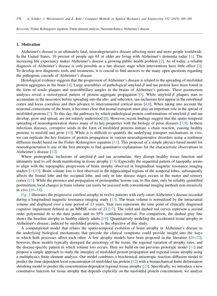
Fig. 1 illustrates the progressive cerebral atrophy in twelve patients with early-onset Alzheimer’s disease recordedduring a longitudinal magnetic resonance imaging study [17]. The brain volume is normalized by the intracranialvolume and displayed over a time period of 13 years. Year zero represents the time point of clinically diagnosedcognitive impairment defined as an MMSE score of 23 [17]. The solid and dashed red curves represent a secondorder polynomial fit to the data points and its 95% confidence interval. For comparison, the dashed gray lineshows the baseline atrophy in healthy elderly adults [19]. Quantitatively modeling the accelerated tissue atrophy inAlzheimer’s disease, induced by misfolded protein, is the objective of this study.
A computational model that relates the spatio-temporal evolution of brain atrophy in Alzheimer’s disease tothe underlying biological mechanisms that precede the clinical symptoms could provide insight into the waysin which both processes affect each other. A few atrophy models have been proposed in the literature [20–22];however, these models typically disregard the anisotropy of the tissue, the regional variation of atrophy rates, andthe disease-specific pattern in which volume loss occurs. Here we build on our previous prototype model [11] andpropose a simple approach to study the interplay of misfolded protein propagation and regional tissue atrophy usinga multiphysics finite element analysis. Our model combines a biochemical anisotropic reaction–diffusion model topredict the time-dependent local concentration of misfolded tau protein [12] with a biomechanical finite deformationshrinking model to predict the concentration-dependent regional tissue atrophy [23]. Specifically, we introduce a newconstitutive function for tissue atrophy that depends explicitly on the misfolded protein concentration, we analyze
A. Schafer, J. Weickenmeier and E. Kuhl / Computer Methods in Applied Mechanics and Engineering 352 (2019) 369–388 371
Fig. 1. Progressive brain atrophy in twelve patients with early-onset Alzheimer’s disease from a longitudinal magnetic resonance imagingstudy [17] compared to baseline atrophy in healthy elderly adults [19]. The brain tissue atrophy is normalized by the intracranial volumeand displayed throughout a period of 13 years. The zero time point represents the onset of clinically diagnosed cognitive impairment withan MMSE score of 23. The solid red curve represents a second order polynomial fit to the data points; the dashed red curves represent the95% confidence interval; the dashed gray line indicates the baseline atrophy in healthy elderly adults.
the nature of coupling between biochemical protein misfolding and biomechanical atrophy, we perform a systematicsensitivity analysis of all atrophy-related model parameters, and calibrate our model to atrophy recordings of patientswith early-onset Alzheimer’s disease. In Section 2, we introduce the governing equations of the coupled proteinspreading and tissue atrophy problems and discuss the nature of coupling. In Section 3, we propose a computationalmodel to solve the protein spreading and tissue atrophy problems using a multiphysics finite element approach andshow how we can implement a discrete version of the governing equations, either in a stand-alone approach or withinexisting nonlinear finite element solvers. In Section 4, we prototype our approach using two-dimensional modelsof the brain that we created from magnetic resonance imaging and tractography data. We perform a systematicsensitivity analysis to study the influence of our model parameters on the spatio-temporal evolution of atrophy andcompare our results to the tissue atrophy curves in early onset Alzheimer’s disease [17] from Fig. 1. Finally, wediscuss our results and provide an outlook towards potential future applications of our model.
2. Continuum modeling of protein spreading and tissue atrophy
Kinematics. We characterize the kinematics of the shrinking brain by the mapping ϕ from the initial configurationB0 to the current configuration Bt at time t . We adopt the conventional notation, x = ϕ(X, t), where x ∈ Bt denotesspatial coordinates, X ∈ B0 material coordinates, t ∈ R+ time. The deformation gradient, F(X, t) = ∇Xϕ(X, t),characterizes local deformations and its determinant, J = det(F), measures the local volume change. To modelbrain atrophy, we adopt the classical multiplicative decomposition of the deformation gradient, F = ∇ϕ, into anelastic part Fe and an atrophy part Fa,
F = ∇ϕ = Fe· Fa and J = det(F) = J e J a. (1)
This multiplicative decomposition carries over to the Jacobian J , where J e= det(Fe) is the elastic volume change
and J a= det(Fa) is the volume loss by tissue atrophy. The elastic part of the deformation Fe contributes to the
elastic strain energy and is fully reversible. The atrophy part Fa defines the tissue loss caused by atrophy anddepends on the local concentration of misfolded protein.
Balance equations of protein spreading. We characterize the spreading of misfolded protein c in the initialconfiguration B0 through a reaction–diffusion equation with a flux Q and a source Fc,
c = Div( Q)+ Fc in B0 , (2)
372 A. Schafer, J. Weickenmeier and E. Kuhl / Computer Methods in Applied Mechanics and Engineering 352 (2019) 369–388
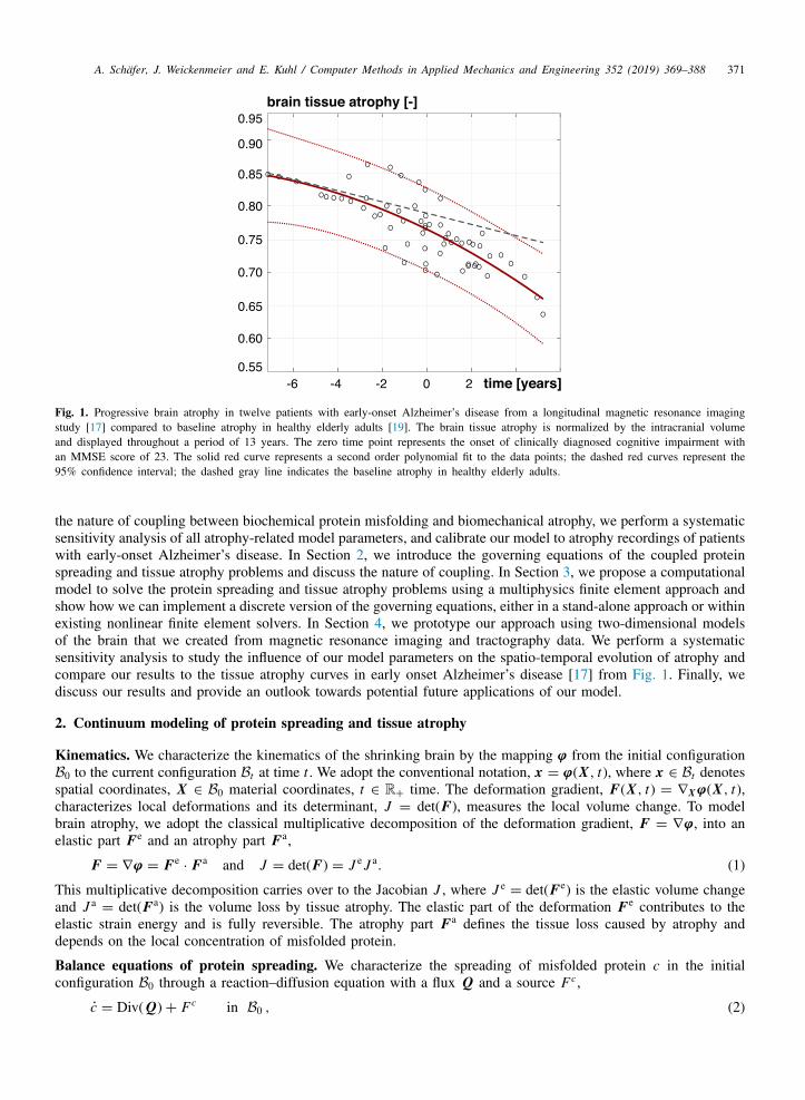
Fig. 2. Kinetics of healthy and misfolded protein. The healthy protein concentration p increases through production k0 and decreases throughclearance k1 and conversion into misfolded protein k12. The misfolded protein concentration p decreases through clearance k1 and increasesthrough conversion from healthy protein k12. The conversion rate k12 collectively represents the recruitment k11′ of healthy protein, itsmisfolding k1′2′ on an infectious seed of misfolded protein, and the fragmentation k2′2 into new infectious seeds.
where c = dc/dt denotes the material time derivative of the misfolded protein concentration c. Using Nanson’sformula, Q = J q · F−t, and the transformation of the source term, Fc
= J f c, we can rephrase thereaction–diffusion equation (2) in the current configuration Bt ,
c = div(J q)+ f c in Bt . (3)
In a continuum sense, the misfolded protein concentration c is an order parameter that varies between 0 ≤ c ≤ 1and characterizes the degree of misfolding. The nature of coupling between the protein spreading problem and thetissue atrophy problem will depend on whether we choose to introduce constitutive equations for the material orspatial flux Q or q and for the material or spatial source Fc or f c.
Balance equations of tissue atrophy. We characterize tissue atrophy through the balance of linear momentum inthe initial configuration B0 in terms of the material divergence of the Piola stress P and the external forces Fϕ ,
0 = Div(P)+ Fϕ in B0 . (4)
Tissue atrophy usually occurs over months, years, or even decades, which allows us to consider the balance oflinear momentum in the quasi-static limit. Similar to the protein spreading problem, we use Nanson’s formula,P = Jσ · F−t, and the relation between the volume forces, Fϕ
= J f ϕ , to transform the material version of themechanical equilibrium equation (4) into its spatial counterpart in the current configuration Bt ,
0 = div(σ )+ f ϕ in Bt , (5)
where σ is the Cauchy stress and f ϕ is the external force vector. For simplicity, we assume that we can neglect theeffect of external forces, Fϕ
= 0 and f ϕ = 0. The material and spatial versions of the tissue atrophy problem (4)and (5) are coupled to the protein spreading problem through the atrophy tensor Fa, which we assume to dependon the local misfolded protein concentration c.
Constitutive equations of protein spreading. For the protein spreading problem, we have to define constitutiveequations for the material or spatial source, either Fc or f c, that represents the growth of misfolded protein and forthe material or spatial flux, either Q or q, that represents the spreading of misfolded protein. Here we introduceboth flux and source in the current, spatial configuration. For the source f c, we adopt our recent protein foldingmodel [12], and assume that the current protein concentration c derives from a kinetic model that balances the totalamount of healthy protein p and misfolded tau protein p,
∂p∂t= k0 − k1 p − k12 p p and
∂ p∂t= −k1 p + k12 p p . (6)
Fig. 2 illustrates the kinetics of healthy and misfolded protein, where k0 is the production rate of healthy proteinp, k1 and k1 are the clearance rates of p and p, and k12 is the conversion rate from the healthy to the misfoldedstate. In the healthy state, the total amount of healthy protein is simply the ratio between production and clearance,p0 = k0/k1. Initially, close to this healthy equilibrium state, the amount of healthy protein is much larger than the
A. Schafer, J. Weickenmeier and E. Kuhl / Computer Methods in Applied Mechanics and Engineering 352 (2019) 369–388 373
amount of misfolded protein, p >> p, which implies that the rate of change of healthy protein is close to zero,∂p/∂t ≈ 0. With these assumptions Eq. ((6).1) provides an explicit estimate for the amount of healthy protein p,
∂p∂t≈ 0 thus p =
k0
k1 + k12 p. (7)
We approximate the amount of healthy protein p using a Taylor series, evaluated at k12/k1 p = 0, to obtainp = k0/k1 [ 1− p k12/k1 ], and substitute this back into Eq. ((6).2) to estimate the amount of misfolded protein,
∂ p∂t=
[k12
k0
k1− k1
]p −
k212 k0
k21
p2 . (8)
For convenience, instead of working with the absolute amount of misfolded protein p, we scale equation (8) bythe maximum amount of misfolded protein pmax
= k1/k12 [ 1 − [k1k1]/[k0k12] ], and re-parameterize equation (8)in terms of the misfolded protein concentration c = p / pmax, which varies between zero and one, 0 ≤ c ≤ 1,
∂c∂t= f c with f c
=
[k12
k0
k1− k1
]c [ 1− c ] . (9)
This definition implies that the spatial reaction or source term f c is directly correlated to the kinetics of misfoldingin Eq. (6): The misfolded protein concentration c increases linearly with the conversion rate from the healthy to themisfolded conformation k12 and with the equilibrium concentration of healthy protein p0 = k0/k1, and decreaseslinearly with the clearance of misfolded protein k1.
Remark 1 (Fisher–Kolmogorov equation). The reaction–diffusion equation for the growth and spreading ofmisfolded proteins (2) with a nonlinear reaction term ((9).2) of α c [1 − c]-type is broadly known as the Fisher–Kolmogorov equation [24,25]. It was originally proposed to model the spreading of a favored gene in populationdynamics, and is now widely used to describe traveling wave solutions in ecology, physiology, combustion,crystallization, plasma physics, and phase transition. Here the parameter α = k12k0/k1 − k1 follows naturally fromthe kinetics of misfolding (6). A characteristic feature of the Fisher–Kolmogorov equation is that the amount ofmisfolded protein, once seeded anywhere in the domain, c > 0, will always increase, c→ 1, and never return backto the benign state, c = 0.
For the flux q, we assume that spreading is driven by the spatial concentration gradient ∇x c and occurs bytwo distinct mechanisms, extracellular diffusion dext, which we associate with the isotropic diffusion through theextracellular space, and axonal transport daxn, which we associate with the local axonal direction n,
J q = d · ∇x c with d = dext i + daxn n⊗ n/λ2n . (10)
Here i is the spatial identity tensor, n/λn = F · n0/λn is the current axonal unit vector, n0 is the initial axonalunit vector that we can determine from diffusion tensor magnetic resonance elastography, and λn = ∥ F · n0 ∥
is its stretch upon deformation. We can rephrase the source J f c= Fc and flux J q = Q · Ft, and introduce the
material source Fc and flux Q in terms of the material concentration gradient ∇X c and the material diffusion tensorD = F−1
· d · F−t,
Fc= J
[k12
k0
k1− k1
]c [ 1− c ] and Q = D · ∇X c with D = dext C−1
+ daxn n0 ⊗ n0/λ2n , (11)
where C = Ft·F is the right Cauchy Green deformation tensor and C−1
= F−1·F−t is its inverse. The constitutive
equation for the flux Q illustrates that the protein spreading problem is constitutively coupled to the tissue atrophyproblem through the deformation-dependent flux Q in Eq. (11) via C−1 and λn = ∥ F · n0 ∥.
Remark 2 (Constitutive decoupling). When defining the source f c in (9) and the flux q in (10) in the currentconfiguration, we introduce an implicit coupling between the protein spreading problem and the tissue atrophyproblem. Alternatively, we could define the source Fc,
Fc=
[k12
k0
k1− k1
]c [ 1− c ] , (12)
374 A. Schafer, J. Weickenmeier and E. Kuhl / Computer Methods in Applied Mechanics and Engineering 352 (2019) 369–388
and the flux Q in the initial configuration as functions of the material diffusion tensor D, the material unit tensorI , the initial axonal unit vector n0, and the material gradient of the concentration ∇X c,
Q = D · ∇X c with D = Dext I + Daxn n0 ⊗ n0 . (13)
We can then rephrase the source Fc= J f c and flux Q = J q · F−t, and introduce the spatial source f c and flux
J q in terms of the spatial concentration gradient ∇x c and the spatial diffusion tensor d = F · D · Ft,
f c=
1J
[k12
k0
k1− k1
]c [ 1− c ] and q =
1J
d · ∇x c with d = Dext b+ Daxn n⊗ n , (14)
where b = F · Ft is the left Cauchy Green deformation tensor. Obviously, the materially defined source (12) andflux (13) are different from the pull back of the spatially defined source and flux (11), and the spatially definedsource (9) and flux (10) are different from the push forward of the materially defined source and flux (14). Themost notable difference is that the materially defined source (12) and flux (13) are deformation independent and nolonger coupled to the tissue atrophy problem. The extent by which the spatially and materially defined fluxes differdepends on the degree of atrophy ϑ and on the time delay between protein misfolding and the onset of atrophy. Inother words, a sufficient time delay between protein misfolding and tissue atrophy would justify using the materialconstitutive equations (12) and (13) and solving the protein spreading and tissue atrophy problems in a decoupledway.
Constitutive equations of tissue atrophy. For the tissue atrophy problem, we have to define constitutive equationsfor the atrophy tensor Fa and the Piola stress P or Cauchy stress σ . We assume that gray matter atrophy is purelyisotropic,
Fa=
3√ϑ I and Fe
= F / 3√ϑ , (15)
and that white matter atrophy is anisotropic and reflects thinning of cortical fiber tracts orthogonal to the fiberdirection n0,
Fa=√ϑ I + [ 1−
√ϑ ] n0 ⊗ n0 and Fe
= F/√ϑ + [1− 1/
√ϑ] n⊗ n0 . (16)
By design, in both cases, ϑ is a measure of the volume loss or tissue shrinkage J a,
ϑ = J a and J e= J / ϑ . (17)
We propose a novel constitutive model for brain atrophy in which the tissue atrophies naturally at a rate G0. Weassume that an increase in misfolded protein c accelerates the progression of natural atrophy by a factor γ (c).For simplicity, we assume that γ (c) is the product of atrophy acceleration Gc/G0 and the Heaviside step functionH(c − ccrit), which activates atrophy acceleration once the misfolded protein concentration c exceeds a criticalthreshold ccrit,
ϑ = [ 1+ γ (c) ] G0 =
{G0 if c < ccrit
G0 + Gc if c ≥ ccrit where γ (c) =Gc
G0H(c − ccrit) . (18)
This implies that we can interpret G0 and Gc as the natural and the misfolding induced atrophy rates. To characterizethe mechanical behavior of the tissue, we introduce the neo-Hookean free energy ψ0 as the atrophy-weighted elasticstored energy ψ , which depends exclusively on the elastic part of the deformation,
ψ0 = J a ψ with ψ = 12 µ [ Fe
: Fe− 3− 2 ln (J e) ]+ 1
2 λ ln2(J e) . (19)
Here µ and λ are the standard Lame parameters that relate to the Young’s modulus E and Poisson’s ratio ν in thelinear limit as λ = Eν/[[1+ν][1−2ν]] and µ = E/[2[1+ν]]. Here we assume µ = 2.07 kPa and λ = 101.43 kPa forgray and µ = 1.15 kPa and λ = 56.35 kPa for white matter [26]. Following standard arguments of thermodynamics,we obtain the Cauchy stress σ ,
σ =1J
dψ0
dF· Ft=
1J e
dψdFe · (Fe)t
=1J e [µ Fe
· (Fe)t+ [ λ ln(J e)− µ ] i ] , (20)
from the neo-Hookean free energy ψ0 in Eq. (19). We emphasize that the Cauchy stress is parameterized exclusivelyin terms of the elastic tensor Fe and its Jacobian J e.
A. Schafer, J. Weickenmeier and E. Kuhl / Computer Methods in Applied Mechanics and Engineering 352 (2019) 369–388 375
3. Computational modeling of protein spreading and tissue atrophy
Continuous residuals. We solve the protein spreading and tissue atrophy problems using the finite element methodand rephrase equations (3) and (5) in their residual forms,
Rc= c − div q − f c .
= 0 in Bt
Rϕ= div σ + fϕ .
= 0 in Bt .(21)
To obtain the weak forms of the residuals (21), we multiply them with the test functions δc and δϕ, integrate themover the domain Bt , perform integration by parts, and use the Neumann boundary conditions.
Spatial and temporal discretizations. In the spirit of the finite element method, we discretize the misfolded proteinconcentration c and the deformation ϕ as global degrees of freedom at the node point level and introduce the degreeof atrophy ϑ as an internal variable on the integration point level. For the spatial discretization, we discretize thedomain Bt into nel finite elements, such that Bt =
⋃nele=1 Be
t . We use C0-continuous shape functions to interpolatethe test and trial functions of the concentration δc and c and of the deformation δϕ and ϕ,
δc =nen∑i=1
N ci δci c =
nen∑k=1
N ck ck δϕ =
nen∑j=1
Nϕ
j δϕ j ϕ =
nen∑l=1
Nϕ
l ϕl (22)
where i, j, k, l sum over the nen element nodes. Although we could technically use different orders of interpolation,here we use the same shape functions N for the concentration c and the deformation ϕ. For the temporaldiscretization, we partition the time interval of interest T into nstep discrete subintervals [ tn, tn+1 ], such thatT =
⋃nstep−1n=0 [ tn, tn+1 ]. We assume that we know the concentration cn , the deformation ϕn , the atrophy ϑn and
all derivable quantities at the beginning of the current interval. In the spirit of implicit time integration schemes,we adopt a finite difference scheme to approximate the evolution of the misfolded protein concentration c in thediscrete residual ((21).1) and the evolution of atrophy ϑ in Eq. (18) as follows,
c = [ c − cn ]/∆t and ϑ = [ϑ − ϑn ]/∆t , (23)
where (◦) and (◦)n denote the unknown quantities at t = tn+1 and tn , and ∆t = t − tn > 0 is the current timeincrement. At the integration point level, for the current concentration c, we evaluate the time-discrete evolution ofthe atrophy, ϑ = ϑn+ [ 1+γ (c) ] G0 ∆t from Eq. (18) with ((23).3), calculate the atrophy tensor Fa and the elastictensor Fe from Eqs. (15) or (16), and determine the Cauchy stress σ from Eq. (20).
Algorithmic residuals. By multiplying the continuous residuals (21) with the test functions δc and δϕ, inte-grating them over the domain Bt , performing integration by parts, and using the spatial (22) and temporal (23)discretizations, we obtain the discrete algorithmic residuals of the protein spreading and tissue atrophy problems,
RcI =
nelA
e=1
∫Be
t
N ci
[c − cn
∆t
]+ ∇x N c
i · q − N ci f c dv .
= 0
Rϕ
J =
nelA
e=1
∫Be
t
∇x Nϕ
j · σ − Nϕ
j f ϕ dv .= 0 ,
(24)
where the operator Anele=1 symbolizes the assembly of the element residuals at the nen element nodes i and j to the
overall residuals at the ngn global nodes I and J .
Linearization. We solve the discrete algorithmic residuals (24) using the incremental iterative Newton–Raphsonmethod and linearize the residuals,
RcI +
ngn∑K=1
KccI K dcK +
ngn∑L=1
KcϕI L · dϕL
.= 0
Rϕ
J +
ngn∑K=1
KϕcJ K dcK +
ngn∑L=1
Kϕϕ
J L · dϕL.= 0
(25)
376 A. Schafer, J. Weickenmeier and E. Kuhl / Computer Methods in Applied Mechanics and Engineering 352 (2019) 369–388
to obtain the iterative update equations for the incremental unknowns dcK and dϕL in terms of the following tangentmoduli,
KccI K =
dRcI
dcK=
nelA
e=1
∫Be
t
N ci
[1∆t
]N c
k +∇x N ci ·
[dq
d∇xc
]· ∇x N c
k + N ci
[d f c
dc
]N c
k dv
KcϕI L =
dRcI
dϕL=
nelA
e=1
∫Be
t
∇x N ci · q ∇x Nϕ
l +∇x N ci ·
[dqdF
]· Ft· ∇x Nϕ
l dv
KϕcJ K =
dRϕ
J
dcK=
nelA
e=1
∫Be
t
∇x Nϕ
j ·
[dσ
dc
]N c
k dv
Kϕϕ
J L =dRϕ
J
dϕL=
nelA
e=1
∫Be
t
∇x Nϕ
j · σ · ∇x Nϕ
l i +∇x Nϕ
j · c · ∇x Nϕ
l dv .
(26)
The concentration moduli KccI K consist of three terms associated with the temporal evolution, the spreading, and the
growth of misfolded protein. The mixed moduli KcϕI L reflect the influence of the deformation ϕ on the spreading of
misfolded protein c, where the first and second terms associated with the geometric and constitutive contributions.The mixed moduli Kϕc
J K reflect the influence of the misfolded protein concentration c on tissue atrophy Fa, whichindirectly influences the elastic tensor Fe, and with it the mechanical stress σ . The mechanical moduli Kϕϕ
J L , similarto the mixed moduli Kcϕ
I L , consist of a geometric and a constitutive contribution, where the latter includes the fourthorder tensor of constitutive moduli c that reflect the dependence of the mechanical stress σ on the deformation ϕ.
From the sensitivities of flux q and source f c with respect to the misfolded protein concentration c and itsgradient ∇xc we obtain the derivatives for the tangent moduli Kcc
I K ,
dqd∇xc
=1J
[ dext i + daxnn⊗ n/λ2n ] and
d f c
dc=
[k12
k0
k1− k1
][ 1− 2c ] . (27)
From the sensitivity of the flux q with respect to the deformation gradient F we obtain the derivative for the tangentmoduli Kcϕ
I L ,
dqdF· Ft=
1J
daxn [ i ⊗ n+ n⊗ i − 2 n⊗ n⊗ n/λn ] · ∇xc ⊗ n/λ2n − q ⊗ i . (28)
From the sensitivity of the Cauchy stress σ with respect to the misfolded protein concentration c, along with theabbreviation A = [dFa/dϑ][dϑ/dc] with either dFa/dϑ = 1/[3 3√
ϑ2] I from (15) or dFa/dϑ = 1/[2√ϑ] [ I −
n0⊗ n0] from (16) and [dϑ/dc] = [dγ /dc] G0 ∆t from (18), we obtain the derivative for the tangent moduli KϕcJ K ,
dσ
dc=
dσ
dFa :dFa
dc= −[Fe
· A · F−1] · σ + [A : (Fa)−t] σ − c : [Fe· A · (Fa)−1] . (29)
From the sensitivity of the Cauchy stress σ with respect to the deformation gradient F along with the associatedsymmetry requirements we obtain the standard fourth-order tensor c of the spatial moduli of the neo-Hookeanmodel for the tangent moduli Kϕϕ
J L ,
c =1J e [i ⊗ Fe] :
∂2ψ
∂Fe⊗ ∂Fe : [i ⊗ (Fe)t] =
1J e [µ− λ ln (J e) ] [ i ⊗ i + i ⊗ i ]+ λ i ⊗ i , (30)
where the component representations of the non-standard fourth-order products expand as {•⊗◦}i jkl = {•}ik⊗{◦} jl
and {•⊗◦}i jkl = {•}il ⊗{◦} jk . For each time increment ∆t , we solve equations (25) for the iterative updates of theglobal unknowns, dc and dϕ, and update the incremental unknowns, ∆c ← ∆c + dc and ∆ϕ ← ∆ϕ + dϕ, untilwe achieve global convergence.
Remark 3 (Constitutive decoupling). Defining the constitutive equation for the spatial flux q rather than the materialflux Q introduces the q and [dq/dF]·Ft terms in the tangent moduli ((26).2). If we define the constitutive equationsfor the material flux Q as functions of the material diffusion tensor D, the initial axonal unit vector n0, and thematerial concentration gradient ∇X c as proposed in (13), the above coupling terms will vanish, and the proteinspreading problem ((24).1) decouples from the tissue atrophy problem ((24).2). We can then solve the proteinspreading problem first, record the concentration c to update the degree of atrophy ϑ using Eq. (18), and then solvethe tissue atrophy problem.
A. Schafer, J. Weickenmeier and E. Kuhl / Computer Methods in Applied Mechanics and Engineering 352 (2019) 369–388 377
Remark 4 (Implementation in Abaqus/Standard). To solve the discrete algorithmic residuals (24), we can use theanalogies of our protein spreading problem (2) or (3) and the classical nonlinear heat transfer problem [27] andinterpret the protein concentration c as temperature scaled to 0 ≤ c ≤ 1, the concentration flux q as heat flux, andthe diffusion tensor d as conductivity tensor, and the nonlinear source f c as heat source. In Abaqus/Standard, wecan add this nonlinear source to the standard heat transfer problem using the subroutine HETVAL, where we definef c= α c [1 − c] and d f c/dc = α [1 − 2 c] with α = k12k0/k1 − k1. We can then solve the protein spreading and
tissue atrophy problems as a coupled problem using a thermo-mechanical formulation with a user-defined subroutineUMAT where we discretize the degree of atrophy ϑ as an internal variable at the integration point level. At eachintegration point, we update the degree of atrophy according to ϑ = ϑn + [ 1 + γ (c) ] G0 ∆t , here specificallyϑ = ϑn + [ G0 + Gc H(c − ccrit) ]∆t from Eq. (18), calculate the atrophy tensor Fa and the elastic tensor Fe
from Eq. (15) or (16), calculate the Cauchy stress σ from Eq. (20), and calculate the sensitivities from Eqs. (27) to(30). However, rather than working directly with the constitutive moduli c from Eq. (30), the user-defined subroutinein Abaqus/Standard utilizes the Jauman rate of the Cauchy stress [27], which requires the following modificationof the tangent moduli, cabaqus
= c+ 12 [ σ ⊗ I + I ⊗ σ + σ ⊗ I + I ⊗ σ ].
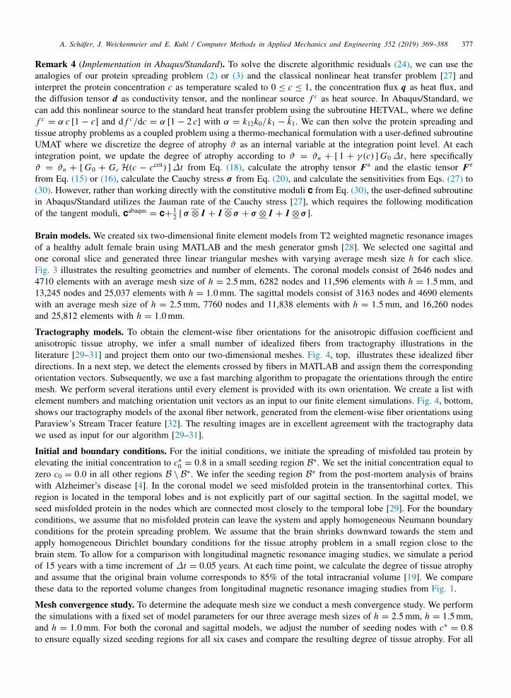
Brain models. We created six two-dimensional finite element models from T2 weighted magnetic resonance imagesof a healthy adult female brain using MATLAB and the mesh generator gmsh [28]. We selected one sagittal andone coronal slice and generated three linear triangular meshes with varying average mesh size h for each slice.Fig. 3 illustrates the resulting geometries and number of elements. The coronal models consist of 2646 nodes and4710 elements with an average mesh size of h = 2.5 mm, 6282 nodes and 11,596 elements with h = 1.5 mm, and13,245 nodes and 25,037 elements with h = 1.0 mm. The sagittal models consist of 3163 nodes and 4690 elementswith an average mesh size of h = 2.5 mm, 7760 nodes and 11,838 elements with h = 1.5 mm, and 16,260 nodesand 25,812 elements with h = 1.0 mm.
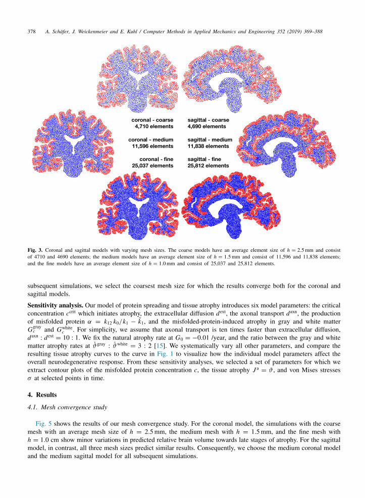
Tractography models. To obtain the element-wise fiber orientations for the anisotropic diffusion coefficient andanisotropic tissue atrophy, we infer a small number of idealized fibers from tractography illustrations in theliterature [29–31] and project them onto our two-dimensional meshes. Fig. 4, top, illustrates these idealized fiberdirections. In a next step, we detect the elements crossed by fibers in MATLAB and assign them the correspondingorientation vectors. Subsequently, we use a fast marching algorithm to propagate the orientations through the entiremesh. We perform several iterations until every element is provided with its own orientation. We create a list withelement numbers and matching orientation unit vectors as an input to our finite element simulations. Fig. 4, bottom,shows our tractography models of the axonal fiber network, generated from the element-wise fiber orientations usingParaview’s Stream Tracer feature [32]. The resulting images are in excellent agreement with the tractography datawe used as input for our algorithm [29–31].
Initial and boundary conditions. For the initial conditions, we initiate the spreading of misfolded tau protein byelevating the initial concentration to c∗0 = 0.8 in a small seeding region B∗. We set the initial concentration equal tozero c0 = 0.0 in all other regions B \ B∗. We infer the seeding region B∗ from the post-mortem analysis of brainswith Alzheimer’s disease [4]. In the coronal model we seed misfolded protein in the transentorhinal cortex. Thisregion is located in the temporal lobes and is not explicitly part of our sagittal section. In the sagittal model, weseed misfolded protein in the nodes which are connected most closely to the temporal lobe [29]. For the boundaryconditions, we assume that no misfolded protein can leave the system and apply homogeneous Neumann boundaryconditions for the protein spreading problem. We assume that the brain shrinks downward towards the stem andapply homogeneous Dirichlet boundary conditions for the tissue atrophy problem in a small region close to thebrain stem. To allow for a comparison with longitudinal magnetic resonance imaging studies, we simulate a periodof 15 years with a time increment of ∆t = 0.05 years. At each time point, we calculate the degree of tissue atrophyand assume that the original brain volume corresponds to 85% of the total intracranial volume [19]. We comparethese data to the reported volume changes from longitudinal magnetic resonance imaging studies from Fig. 1.
Mesh convergence study. To determine the adequate mesh size we conduct a mesh convergence study. We performthe simulations with a fixed set of model parameters for our three average mesh sizes of h = 2.5 mm, h = 1.5 mm,and h = 1.0 mm. For both the coronal and sagittal models, we adjust the number of seeding nodes with c∗ = 0.8to ensure equally sized seeding regions for all six cases and compare the resulting degree of tissue atrophy. For all
378 A. Schafer, J. Weickenmeier and E. Kuhl / Computer Methods in Applied Mechanics and Engineering 352 (2019) 369–388
Fig. 3. Coronal and sagittal models with varying mesh sizes. The coarse models have an average element size of h = 2.5 mm and consistof 4710 and 4690 elements; the medium models have an average element size of h = 1.5 mm and consist of 11,596 and 11,838 elements;and the fine models have an average element size of h = 1.0 mm and consist of 25,037 and 25,812 elements.
subsequent simulations, we select the coarsest mesh size for which the results converge both for the coronal andsagittal models.
Sensitivity analysis. Our model of protein spreading and tissue atrophy introduces six model parameters: the criticalconcentration ccrit which initiates atrophy, the extracellular diffusion dext, the axonal transport daxn, the productionof misfolded protein α = k12 k0/k1 − k1, and the misfolded-protein-induced atrophy in gray and white matterGgray
c and Gwhitec . For simplicity, we assume that axonal transport is ten times faster than extracellular diffusion,
daxn: dext
= 10 : 1. We fix the natural atrophy rate at G0 = −0.01 /year, and the ratio between the gray and whitematter atrophy rates at ϑgray
: ϑwhite= 3 : 2 [15]. We systematically vary all other parameters, and compare the
resulting tissue atrophy curves to the curve in Fig. 1 to visualize how the individual model parameters affect theoverall neurodegenerative response. From these sensitivity analyses, we selected a set of parameters for which weextract contour plots of the misfolded protein concentration c, the tissue atrophy J a
= ϑ , and von Mises stressesσ at selected points in time.
4. Results
4.1. Mesh convergence study
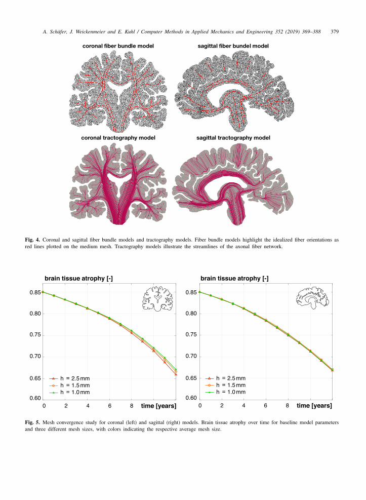
Fig. 5 shows the results of our mesh convergence study. For the coronal model, the simulations with the coarsemesh with an average mesh size of h = 2.5 mm, the medium mesh with h = 1.5 mm, and the fine mesh withh = 1.0 cm show minor variations in predicted relative brain volume towards late stages of atrophy. For the sagittalmodel, in contrast, all three mesh sizes predict similar results. Consequently, we choose the medium coronal modeland the medium sagittal model for all subsequent simulations.
A. Schafer, J. Weickenmeier and E. Kuhl / Computer Methods in Applied Mechanics and Engineering 352 (2019) 369–388 379
Fig. 4. Coronal and sagittal fiber bundle models and tractography models. Fiber bundle models highlight the idealized fiber orientations asred lines plotted on the medium mesh. Tractography models illustrate the streamlines of the axonal fiber network.
Fig. 5. Mesh convergence study for coronal (left) and sagittal (right) models. Brain tissue atrophy over time for baseline model parametersand three different mesh sizes, with colors indicating the respective average mesh size.
380 A. Schafer, J. Weickenmeier and E. Kuhl / Computer Methods in Applied Mechanics and Engineering 352 (2019) 369–388
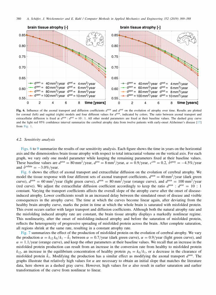
Fig. 6. Influence of the axonal transport and diffusion coefficients daxn and dext on the evolution of atrophy over time. Results are plottedfor coronal (left) and sagittal (right) models and four different values for daxn, indicated by colors. The ratio between axonal transport andextracellular diffusion is fixed at daxn
: dext= 10 : 1. All other model parameters are fixed at their baseline values. The dashed gray curve
and the light red 95% confidence interval summarize the cerebral atrophy data from twelve patients with early-onset Alzheimer’s disease [17]from Fig. 1.
4.2. Sensitivity analysis
Figs. 6 to 9 summarize the results of our sensitivity analysis. Each figure shows the time in years on the horizontalaxis and the dimensionless brain tissue atrophy with respect to total intracranial volume on the vertical axis. For eachgraph, we vary only one model parameter while keeping the remaining parameters fixed at their baseline values.These baseline values are daxn
= 80 mm2/year, dext= 8 mm2/year, α = 0.9/year, ccrit
= 0.2, ϑgray= −4.5%/year
and ϑwhite= −3.0%/year.
Fig. 6 shows the effect of axonal transport and extracellular diffusion on the evolution of cerebral atrophy. Wemodel the tissue response with four different sets of axonal transport coefficients, daxn
= 40 mm2/year (dark greencurve), daxn
= 60 mm2/year (light green curve), daxn= 80 mm2/year (orange curve), and daxn
= 100 mm2/year(red curve). We adjust the extracellular diffusion coefficient accordingly to keep the ratio daxn
: dext= 10 : 1
constant. Varying the transport coefficients affects the overall slope of the atrophy curve after the onset of disease-induced atrophy. Lower coefficients result in an increased delay between the simulated onset of disease and visibleconsequences in the atrophy curve. The time at which the curves become linear again, after deviating from thehealthy brain atrophy curve, marks the point in time at which the whole brain is saturated with misfolded protein.This event occurs earlier with larger transport and diffusion coefficients. Although both the natural atrophy rate andthe misfolding induced atrophy rate are constant, the brain tissue atrophy displays a markedly nonlinear regime.This nonlinearity, after the onset of misfolding-induced atrophy and before the saturation of misfolded protein,reflects the heterogeneity of progressive spreading of misfolded protein across the brain. After complete saturation,all regions shrink at the same rate, resulting in a constant atrophy rate.
Fig. 7 summarizes the effect of the production of misfolded protein on the evolution of cerebral atrophy. We varythe production α = k12 k0/k1− k1 between α = 0.7/year (dark green curve), α = 0.9/year (light green curve), andα = 1.1/year (orange curve), and keep the other parameters at their baseline values. We recall that an increase in themisfolded protein production can result from an increase in the conversion rate from healthy to misfolded proteink12, an increase in the equilibrium concentration of healthy protein p0 = k0/k1, or a decrease in the clearance ofmisfolded protein k1. Modifying the production has a similar effect as modifying the axonal transport daxn. Thegraphs illustrate that relatively high values for α are necessary to obtain an initial slope that matches the literaturedata, here shown as a dashed gray curve. However, high values for α also result in earlier saturation and earliertransformation of the curve from nonlinear to linear.
A. Schafer, J. Weickenmeier and E. Kuhl / Computer Methods in Applied Mechanics and Engineering 352 (2019) 369–388 381
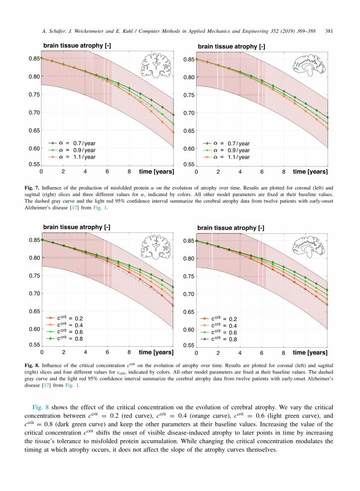
Fig. 7. Influence of the production of misfolded protein α on the evolution of atrophy over time. Results are plotted for coronal (left) andsagittal (right) slices and three different values for α, indicated by colors. All other model parameters are fixed at their baseline values.The dashed gray curve and the light red 95% confidence interval summarize the cerebral atrophy data from twelve patients with early-onsetAlzheimer’s disease [17] from Fig. 1.
Fig. 8. Influence of the critical concentration ccrit on the evolution of atrophy over time. Results are plotted for coronal (left) and sagittal(right) slices and four different values for ccrit, indicated by colors. All other model parameters are fixed at their baseline values. The dashedgray curve and the light red 95% confidence interval summarize the cerebral atrophy data from twelve patients with early-onset Alzheimer’sdisease [17] from Fig. 1.
Fig. 8 shows the effect of the critical concentration on the evolution of cerebral atrophy. We vary the criticalconcentration between ccrit
= 0.2 (red curve), ccrit= 0.4 (orange curve), ccrit
= 0.6 (light green curve), andccrit= 0.8 (dark green curve) and keep the other parameters at their baseline values. Increasing the value of the
critical concentration ccrit shifts the onset of visible disease-induced atrophy to later points in time by increasingthe tissue’s tolerance to misfolded protein accumulation. While changing the critical concentration modulates thetiming at which atrophy occurs, it does not affect the slope of the atrophy curves themselves.
382 A. Schafer, J. Weickenmeier and E. Kuhl / Computer Methods in Applied Mechanics and Engineering 352 (2019) 369–388
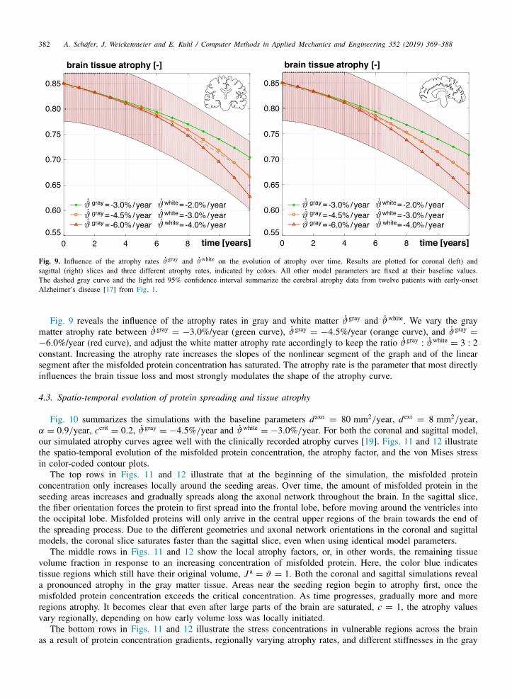
Fig. 9. Influence of the atrophy rates ϑgray and ϑwhite on the evolution of atrophy over time. Results are plotted for coronal (left) andsagittal (right) slices and three different atrophy rates, indicated by colors. All other model parameters are fixed at their baseline values.The dashed gray curve and the light red 95% confidence interval summarize the cerebral atrophy data from twelve patients with early-onsetAlzheimer’s disease [17] from Fig. 1.
Fig. 9 reveals the influence of the atrophy rates in gray and white matter ϑgray and ϑwhite. We vary the graymatter atrophy rate between ϑgray
= −3.0%/year (green curve), ϑgray= −4.5%/year (orange curve), and ϑgray
=
−6.0%/year (red curve), and adjust the white matter atrophy rate accordingly to keep the ratio ϑgray: ϑwhite
= 3 : 2constant. Increasing the atrophy rate increases the slopes of the nonlinear segment of the graph and of the linearsegment after the misfolded protein concentration has saturated. The atrophy rate is the parameter that most directlyinfluences the brain tissue loss and most strongly modulates the shape of the atrophy curve.
4.3. Spatio-temporal evolution of protein spreading and tissue atrophy
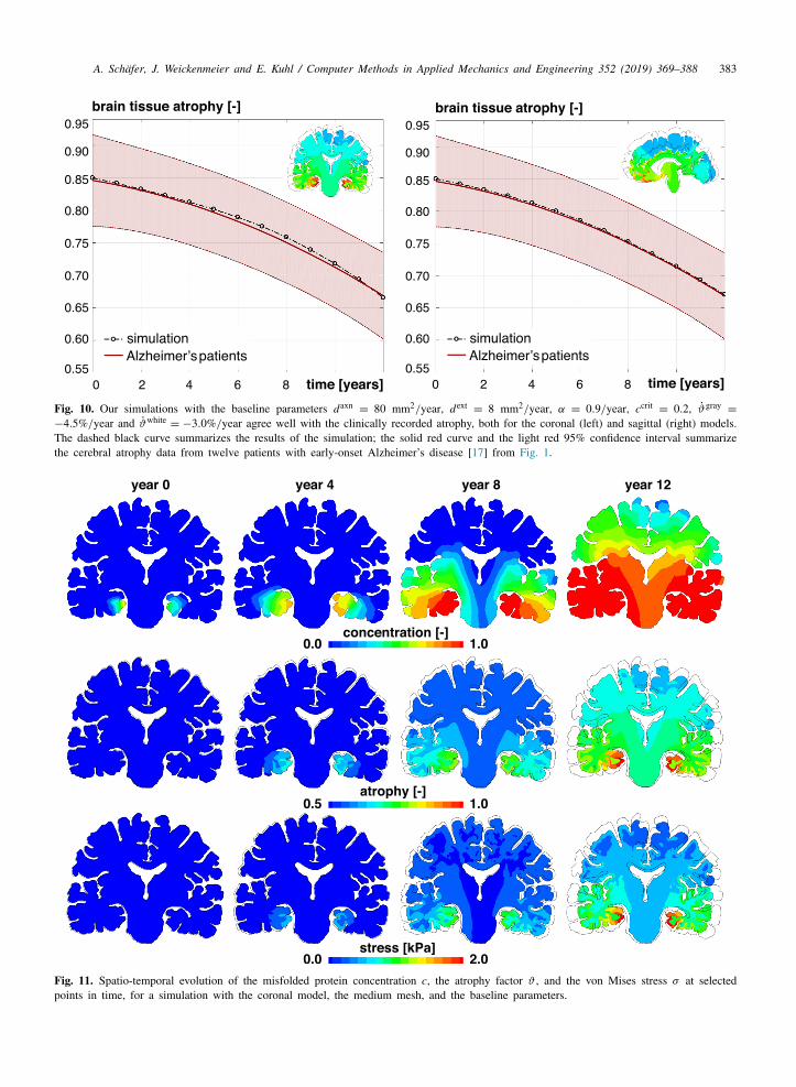
Fig. 10 summarizes the simulations with the baseline parameters daxn= 80 mm2/year, dext
= 8 mm2/year,α = 0.9/year, ccrit
= 0.2, ϑgray= −4.5%/year and ϑwhite
= −3.0%/year. For both the coronal and sagittal model,our simulated atrophy curves agree well with the clinically recorded atrophy curves [19]. Figs. 11 and 12 illustratethe spatio-temporal evolution of the misfolded protein concentration, the atrophy factor, and the von Mises stressin color-coded contour plots.
The top rows in Figs. 11 and 12 illustrate that at the beginning of the simulation, the misfolded proteinconcentration only increases locally around the seeding areas. Over time, the amount of misfolded protein in theseeding areas increases and gradually spreads along the axonal network throughout the brain. In the sagittal slice,the fiber orientation forces the protein to first spread into the frontal lobe, before moving around the ventricles intothe occipital lobe. Misfolded proteins will only arrive in the central upper regions of the brain towards the end ofthe spreading process. Due to the different geometries and axonal network orientations in the coronal and sagittalmodels, the coronal slice saturates faster than the sagittal slice, even when using identical model parameters.
The middle rows in Figs. 11 and 12 show the local atrophy factors, or, in other words, the remaining tissuevolume fraction in response to an increasing concentration of misfolded protein. Here, the color blue indicatestissue regions which still have their original volume, J a
= ϑ = 1. Both the coronal and sagittal simulations reveala pronounced atrophy in the gray matter tissue. Areas near the seeding region begin to atrophy first, once themisfolded protein concentration exceeds the critical concentration. As time progresses, gradually more and moreregions atrophy. It becomes clear that even after large parts of the brain are saturated, c = 1, the atrophy valuesvary regionally, depending on how early volume loss was locally initiated.
The bottom rows in Figs. 11 and 12 illustrate the stress concentrations in vulnerable regions across the brainas a result of protein concentration gradients, regionally varying atrophy rates, and different stiffnesses in the gray
A. Schafer, J. Weickenmeier and E. Kuhl / Computer Methods in Applied Mechanics and Engineering 352 (2019) 369–388 383
Fig. 10. Our simulations with the baseline parameters daxn= 80 mm2/year, dext
= 8 mm2/year, α = 0.9/year, ccrit= 0.2, ϑgray
=
−4.5%/year and ϑwhite= −3.0%/year agree well with the clinically recorded atrophy, both for the coronal (left) and sagittal (right) models.
The dashed black curve summarizes the results of the simulation; the solid red curve and the light red 95% confidence interval summarizethe cerebral atrophy data from twelve patients with early-onset Alzheimer’s disease [17] from Fig. 1.
Fig. 11. Spatio-temporal evolution of the misfolded protein concentration c, the atrophy factor ϑ , and the von Mises stress σ at selectedpoints in time, for a simulation with the coronal model, the medium mesh, and the baseline parameters.
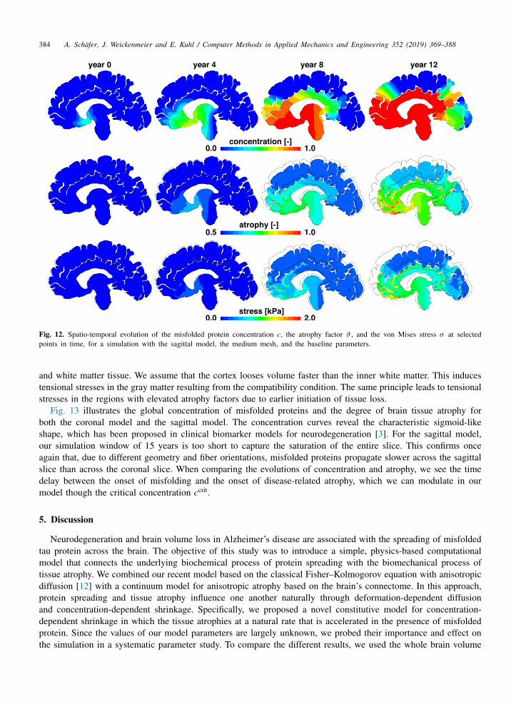
384 A. Schafer, J. Weickenmeier and E. Kuhl / Computer Methods in Applied Mechanics and Engineering 352 (2019) 369–388
Fig. 12. Spatio-temporal evolution of the misfolded protein concentration c, the atrophy factor ϑ , and the von Mises stress σ at selectedpoints in time, for a simulation with the sagittal model, the medium mesh, and the baseline parameters.
and white matter tissue. We assume that the cortex looses volume faster than the inner white matter. This inducestensional stresses in the gray matter resulting from the compatibility condition. The same principle leads to tensionalstresses in the regions with elevated atrophy factors due to earlier initiation of tissue loss.
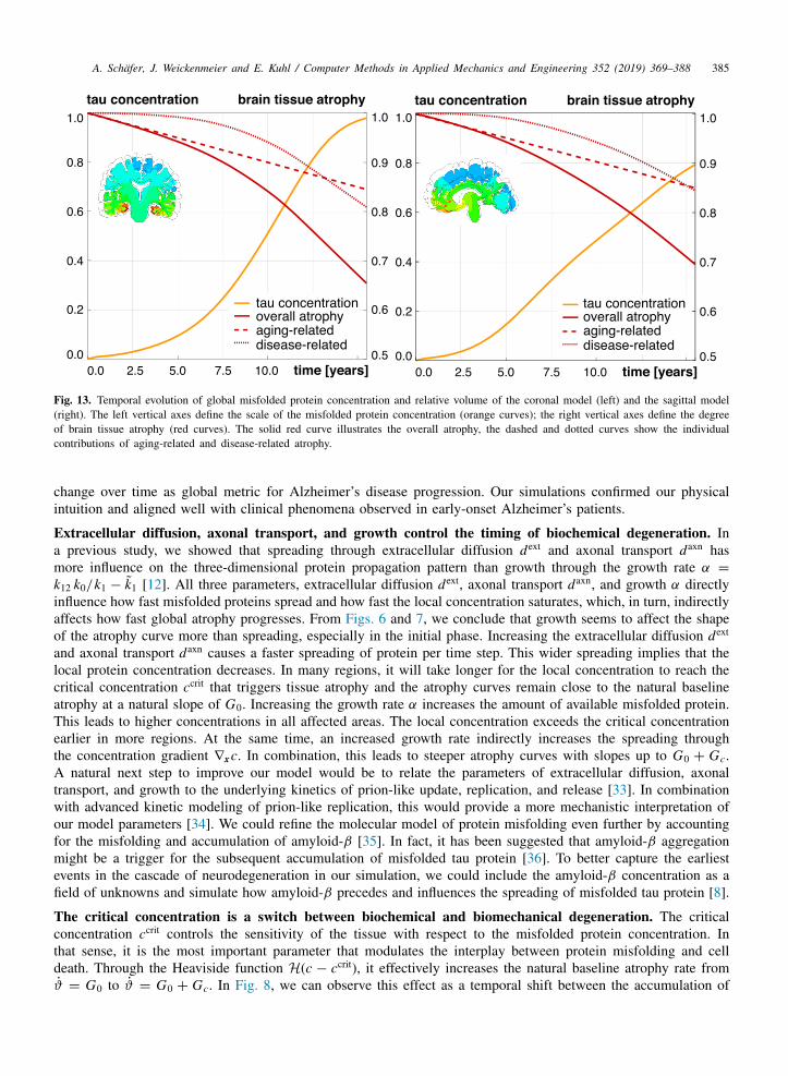
Fig. 13 illustrates the global concentration of misfolded proteins and the degree of brain tissue atrophy forboth the coronal model and the sagittal model. The concentration curves reveal the characteristic sigmoid-likeshape, which has been proposed in clinical biomarker models for neurodegeneration [3]. For the sagittal model,our simulation window of 15 years is too short to capture the saturation of the entire slice. This confirms onceagain that, due to different geometry and fiber orientations, misfolded proteins propagate slower across the sagittalslice than across the coronal slice. When comparing the evolutions of concentration and atrophy, we see the timedelay between the onset of misfolding and the onset of disease-related atrophy, which we can modulate in ourmodel though the critical concentration ccrit.
5. Discussion
Neurodegeneration and brain volume loss in Alzheimer’s disease are associated with the spreading of misfoldedtau protein across the brain. The objective of this study was to introduce a simple, physics-based computationalmodel that connects the underlying biochemical process of protein spreading with the biomechanical process oftissue atrophy. We combined our recent model based on the classical Fisher–Kolmogorov equation with anisotropicdiffusion [12] with a continuum model for anisotropic atrophy based on the brain’s connectome. In this approach,protein spreading and tissue atrophy influence one another naturally through deformation-dependent diffusionand concentration-dependent shrinkage. Specifically, we proposed a novel constitutive model for concentration-dependent shrinkage in which the tissue atrophies at a natural rate that is accelerated in the presence of misfoldedprotein. Since the values of our model parameters are largely unknown, we probed their importance and effect onthe simulation in a systematic parameter study. To compare the different results, we used the whole brain volume
A. Schafer, J. Weickenmeier and E. Kuhl / Computer Methods in Applied Mechanics and Engineering 352 (2019) 369–388 385
Fig. 13. Temporal evolution of global misfolded protein concentration and relative volume of the coronal model (left) and the sagittal model(right). The left vertical axes define the scale of the misfolded protein concentration (orange curves); the right vertical axes define the degreeof brain tissue atrophy (red curves). The solid red curve illustrates the overall atrophy, the dashed and dotted curves show the individualcontributions of aging-related and disease-related atrophy.
change over time as global metric for Alzheimer’s disease progression. Our simulations confirmed our physicalintuition and aligned well with clinical phenomena observed in early-onset Alzheimer’s patients.
Extracellular diffusion, axonal transport, and growth control the timing of biochemical degeneration. Ina previous study, we showed that spreading through extracellular diffusion dext and axonal transport daxn hasmore influence on the three-dimensional protein propagation pattern than growth through the growth rate α =k12 k0/k1 − k1 [12]. All three parameters, extracellular diffusion dext, axonal transport daxn, and growth α directlyinfluence how fast misfolded proteins spread and how fast the local concentration saturates, which, in turn, indirectlyaffects how fast global atrophy progresses. From Figs. 6 and 7, we conclude that growth seems to affect the shapeof the atrophy curve more than spreading, especially in the initial phase. Increasing the extracellular diffusion dext
and axonal transport daxn causes a faster spreading of protein per time step. This wider spreading implies that thelocal protein concentration decreases. In many regions, it will take longer for the local concentration to reach thecritical concentration ccrit that triggers tissue atrophy and the atrophy curves remain close to the natural baselineatrophy at a natural slope of G0. Increasing the growth rate α increases the amount of available misfolded protein.This leads to higher concentrations in all affected areas. The local concentration exceeds the critical concentrationearlier in more regions. At the same time, an increased growth rate indirectly increases the spreading throughthe concentration gradient ∇xc. In combination, this leads to steeper atrophy curves with slopes up to G0 + Gc.A natural next step to improve our model would be to relate the parameters of extracellular diffusion, axonaltransport, and growth to the underlying kinetics of prion-like update, replication, and release [33]. In combinationwith advanced kinetic modeling of prion-like replication, this would provide a more mechanistic interpretation ofour model parameters [34]. We could refine the molecular model of protein misfolding even further by accountingfor the misfolding and accumulation of amyloid-β [35]. In fact, it has been suggested that amyloid-β aggregationmight be a trigger for the subsequent accumulation of misfolded tau protein [36]. To better capture the earliestevents in the cascade of neurodegeneration in our simulation, we could include the amyloid-β concentration as afield of unknowns and simulate how amyloid-β precedes and influences the spreading of misfolded tau protein [8].
The critical concentration is a switch between biochemical and biomechanical degeneration. The criticalconcentration ccrit controls the sensitivity of the tissue with respect to the misfolded protein concentration. Inthat sense, it is the most important parameter that modulates the interplay between protein misfolding and celldeath. Through the Heaviside function H(c − ccrit), it effectively increases the natural baseline atrophy rate fromϑ = G0 to ϑ = G0 + Gc. In Fig. 8, we can observe this effect as a temporal shift between the accumulation of
386 A. Schafer, J. Weickenmeier and E. Kuhl / Computer Methods in Applied Mechanics and Engineering 352 (2019) 369–388
misfolded protein and the onset of atrophy. An important future direction is the acquisition of quantitative knowledgeabout the relation between the two time scales of misfolded tau protein progression on the one hand and atrophypropagation on the other hand [35]. Since the biochemical processes of neurodegeneration precede the clinicaldiagnosis in Alzheimer’s disease patients often by one or two decades this is a challenging task and most reportedfindings are hypothetical or qualitative at best [3,37]. Despite the lack of quantitative information, our model caneasily account for varying temporal offsets between the protein spreading and tissue atrophy problems by adjustingequation (18), either by simply varying the critical concentration ccrit or by replacing the atrophy acceleration γ (c).To date, it is unknown how much protein misfolding is too much protein misfolding for the cell to survive. Froma modeling perspective, answering this question has important implications on the nature of coupling betweenbiochemical and biomechanical degeneration. If the temporal shift between protein misfolding and tissue atrophyis large enough, the two problems naturally decouple and we can solve for protein misfolding first, store the timetcrit at which each integration point reaches the critical concentration ccrit, and then solve for tissue atrophy. Herewe selected a value of ccrit
= 0.2 as baseline value for our simulations. Once future experimental investigationsreveal more quantitative information, we can easily change and adjust this value, or even change the amplificationfunction, γ = Gc/G0 H(c − ccrit), entirely. For example, instead of using the concentration only implicitly as aswitch in the Heaviside function H(c− ccrit), we could scale atrophy acceleration explicitly with the concentrationitself, γ = Gc/G0 c. The inherent modularity of our model, especially with a view towards the biochemical andbiomechanical coupling, will easily allow us to adjust the model to potential future findings, which could potentiallyemerge from positron emission tomography imaging of patients with familial or sporadic Alzheimer’s disease.
The interplay of natural atrophy and misfolding-induced atrophy modulates biomechanical degeneration.The extracellular diffusion, axonal transport, and growth govern the timing of protein spreading whereas the criticalconcentration governs the time delay between the biomarkers of protein misfolding and tissue atrophy. In contrast,the tissue atrophy rates ϑgray
= G0 + Ggrayc and ϑwhite
= G0 + Gwhitec only affect the biomechanical side of the
problem. Varying these rates only affects the speed by which each affected element shrinks, but not the size ofthe activated domain. Changing their ratio Ggray
c : Gwhitec , however, can generate different shrinkage patterns as we
have previously shown [23]. Interestingly, we achieve a good fit for both, the coronal and the sagittal model, withidentical model parameters in Fig. 9. This suggests that our atrophy model for neurodegeneration (18), ϑ = G0+Gc,in which atrophy is a result of the natural baseline atrophy rate G0 and the misfolding induced atrophy rate Gc isa reasonable first approximation. The simulated curve becomes linear too early compared to the clinically reportedcurve [19]. However, a numerical fitting addressing these disparities will only make sense with a three dimensionalwhole brain geometry. Only then, a quantitative comparison with the literature data, in which volume and not areachange is evaluated, can be made.
The predicted spatio-temporal patterns of degeneration mimic staging in the neurodegenerative disorders.After our systematic sensitivity analysis, we conclude that an axonal transport of daxn
= 80 mm2/year, anextracellular diffusion of dext
= 8 mm2/year, a growth rate of α = 0.9, a critical concentration of ccrit= 0.2,
and atrophy rates of ϑgray= −4.5%/year and ϑwhite
= −3.0%/year provide reasonable predictions of proteinspreading and tissue atrophy. Our protein propagation patterns in Figs. 11 and 13, top, agree well with the stagingsequence inferred from postmortem analyses [4,7]. Similar to biochemical degeneration, biomechanical degenerationfirst develops in the hippocampal periphery and then spreads throughout the temporal lobes and into the frontallobe [15]. The occipital lobe is affected next, while the central areas comprising motor and sensory cortex aremainly spared. Not only our global atrophy curves in Fig. 10, but also the spatio-temporal patterns of atrophy inFigs. 11 and 13, middle, agree well with the observed timeline and sequence of degeneration. An important featureof our model is that it predicts regionally-varying degrees of atrophy across the brain, even after the entire braingeometry is saturated with misfolded protein. Modeling volume loss as a dynamic process that is initiated beyonda critical concentration and increases progressively in time naturally captures these observed characteristics [37].Our model also nicely predicts a widening of the cerebral sulci, both in the coronal slice in Fig. 11 and in thesagittal slice in Fig. 13, a common feature of atrophy as evidenced through magnetic resonance imaging [38].Another common observation associated with cerebral atrophy is the progressive increase in ventricular volumes,a feature that is not yet captured to full extent by our model. To better capture this effect, in the future, we willinvestigate the interplay of biochemical and fluid mechanical factors and include those effects in our model [39].The stress distributions in Figs. 10 and 11, bottom, reveal elevated stresses due to regionally differential atrophy.
A. Schafer, J. Weickenmeier and E. Kuhl / Computer Methods in Applied Mechanics and Engineering 352 (2019) 369–388 387
Elevated stresses occur in regions of pronounced stiffness and shrinkage gradients, primarily located at the interfacebetween gray and white matter, in the depth of the cerebral sulci. These stress concentrations could potentiallyamplify protein misfolding or cause additional damage to the tissue [23]. A natural next step would be to simulatethe interplay between protein spreading and tissue atrophy with a fully three-dimensional whole brain model. Wehave already made a first promising step in this direction and registered fiber orientations from diffusion tensorimaging on a three-dimensional finite element model of a healthy adult human brain [12]. While two-dimensionalsimulations provide excellent insight into the underlying phenomena, the role of the model parameters, and thenature of coupling between biochemistry and biomechanics [40], real three-dimensional simulations would providea more realistic basis for the comparison with literature values on observed volume changes in time.
6. Conclusion
We proposed a multiphysics model that couples misfolded protein spreading and tissue atrophy to explore thespatio-temporal interplay of biochemical and biomechanical degeneration in Alzheimer’s disease. Our predictedspatio-temporal patterns of protein spreading and tissue atrophy agree well with clinical observations inferred fromin-vivo magnetic resonance imaging and post-mortem histopathology. Specifically, we observed high concentrationsof misfolded protein and pronounced tissue atrophy in regions near the hippocampus. A critical link betweenbiochemical and biomechanical degeneration is the rate of cerebral atrophy. This atrophy rate mimics both, naturalaging-induced atrophy and accelerated misfolding-induced atrophy. Our simulations suggest that protein misfoldingcan accelerate natural atrophy between three- and five-fold. From a basic science point of view, computationalmodeling can improve our general understanding of the interplay between disease progression on the molecular andcellular scales on the one hand and atrophy progression on the tissue and organ scales on the other hand. From atranslational point of view, once appropriately calibrated and validated, computational models of neurodegenerationcould help improve diagnostic tools, advance early detection, and, ultimately, enable early interventions to delaythe onset of cognitive decline in familial or sporadic Alzheimer’s disease.
Acknowledgments
This work was supported by the Stanford Bio-X IIP seed grant “Molecular mechanisms of Chronic TraumaticEncephalopathy” and the National Science Foundation grant CMMI 1727268 “Understanding neurodegenerationacross the scales”.
References[1] Alzheimer’s Association, 2018. 2018 Alzheimer’s disease facts and figures. Alzheimer’s & Dementia 14, 367-429.[2] L.E. Hebert, L.A. Beckett, P.A. Scherr, D.A. Evans, Annual incidence of Alzheimer disease in the United States projected to the years
2000 through 2050, Alzheimer Dis. Assoc. Disorders 15 (2001) 169–173.[3] C.R. Jack, D.M. Holtzman, Biomarker modeling of Alzheimer’s disease, Neuron 80 (2013) 1347–1358.[4] H. Braak, E. Braak, Neuropathological staging of Alzheimer-related changes, Acta Neuropathologica 82 (1991) 239–259.[5] H. Braak, E. Braak, Frequencey of stages of Alzheimer-related lesions in different age categories, Neurobiol. Aging 18 (1997) 351–357.[6] D.R. Thal, U. Rub, M. Orantes, H. Braak, Phases of A beta-deposition in the human brain and its relevance for the development of
AD, Neurology 58 (2002) 1791–1800.[7] M. Jucker, L.C. Walker, Pathological protein seeding in alzheimer disease and other neurodegenerative disorders, Ann. Neurol. 70
(2011) 532–540.[8] M. Jucker, L.C. Walker, Propagation and spread of pathogenic protein assemblies in neurodegenerative diseases, Nature Neurosci. 21
(2018) 1341–1349.[9] M. Jucker, L.C. Walker, Self-propagation of pathogenic protein aggregates in neurodegenerative diseases, Nature 501 (2013) 45–51.
[10] S.B. Prusiner, Prions. Nobel lecture, Proc. Natl. Acad. Sci. 95 (1998) 13363–13383.[11] J. Weickenmeier, E. Kuhl, A. Goriely, The multiphysics of prion-like diseases: progression and atrophy, Phys. Rev. Lett. 121 (2018)
158101.[12] J. Weickenmeier, M. Jucker, A. Goriely, E. Kuhl, A physics-based model explains the prion-like features of neurodegeneration in
Alzheimers disease, parkinsons disease, and amyotrophic lateral sclerosis, J. Mech. Phys. Solids 124 (2019) 264–281.[13] G.B. Stokin, L.S. Goldstein, Axonal transport and Alzheimer’s disease, Annu. Rev. Biochem. 75 (2006) 607–627.[14] A. Raj, A. Kuceyeski, M. Weiner, A network diffusion model of disease progression in dementia, Neuron 73 (2012) 1204–1215.[15] P.M. Thompson, K.M. Hayashi, G. De Zubicaray, A.L. Janke, S.E. Rose, J. Semple, D. Herman, M.S. Hong, S.S. Dittmer, D.M.
Doddrell, A.W. Toga, Dynamics of gray matter loss in Alzheimer’s disease, J. Neurosci. 23 (2003) 994–1005.[16] N.C. Fox, W.R. Crum, R.I. Scahill, J.M. Stevens, J.C. Janssen, M.N. Rossor, Imaging of onset and progression of Alzheimer’s disease
with voxel-compression mapping of serial magnetic resonance images, Lancet 358 (2001) 201–205.
388 A. Schafer, J. Weickenmeier and E. Kuhl / Computer Methods in Applied Mechanics and Engineering 352 (2019) 369–388
[17] D. Chan, J.C. Janssen, J.L. Whitwell, H.C. Watt, R. Jenkins, C. Frost, M.N. Rossor, N.C. Fox, Change in rates of cerebral atrophyover time in early-onset alzheimer’s disease: longitudinal MRI study, Lancet 362 (2003) 1121–1122.
[18] B.H. Ridha, J. Barnes, J.W. Bartlett, A. Godbolt, T. Pepple, M.N. Rossor, N.C. Fox, Tracking atrophy progression in familial Alzheimer’sdisease: a serial MRI study, Lancet Neurol. 5 (2006) 828–834.
[19] J.L. Whitwell, W.R. Crum, H.C. Watt, N.C. Fox, Normalization of cerebral volumes by use of intracranial volume: implications forlongitudinal quantitative MR imaging, Amer. J. Neuroradiol. 22 (2001) 1483–1489.
[20] O. Camara, M. Schweiger, R.I. Scahill, W.R. Crum, B.I. Sneller, J.A. Schnabel, G.R. Ridgway, D.M. Cash, D.L. Hill, N.C. Fox,Phenomenological model of diffuse global and regional atrophy using finite-element methods, IEEE Trans. Med. Imaging 25 (2006)1417–1430.
[21] B. Karacali, C. Davatzikos, Simulation of tissue atrophy using a topology preserving transformation model, IEEE Trans. Med. Imaging25 (2006) 649–652.
[22] A.D.C. Smith, W.R. Crum, D.L. Hill, N.A. Thacker, P.A. Bromiley, Biomechanical simulation of atrophy in MR images, in: MedicalImaging 2003: Image Processing (5032), 2003, pp. 481–491.
[23] T.C. Harris, R. de Rooij, E. Kuhl, The shrinking brain: Cerebral atrophy following traumatic brain injury, Ann. Biomed. Eng. (2018)http://dx.doi.org/10.1007/s10439-018-02148-2.
[24] R.A. Fisher, The wave of advance of advantageous genes, Ann. Eugenics 7 (1937) 355–369.[25] A.N. Kolmogorov, I.G. Petrovsky, N.S. Piskunov, Investigation of the equation of diffusion combined with increasing of the substance
and its application to a biology problem, Bull. Moscow State Univ. Ser. A Math. Mech. 1 (1937) 1–25.[26] S. Budday, G. Sommer, C. Birkl, C. Langkammer, J. Haybaeck, J. Kohnert, M. Bauer, F. Paulsen, P. Steinmann, E. Kuhl, G.A.
Holzapfel, Mechanical characterization of human brain tissue, Acta Biomater. 48 (2017) 319–340.[27] Abaqus 6.14. Analysis User’s Manual. SIMULIA. Dassault Systèmes. 2014.[28] C. Geuzaine, J.F. Remacle, Gmsh: A 3-D finite element mesh generator with built-in pre- and post-processing facilities, Internat. J.
Numer. Methods Engrg. 79 (2009) 1309–1331.[29] L. Concha, D.W. Gross, C. Beaulieu, Diffusion tensor tractography of the limbic system, Amer. J. Neuroradiol. 26 (2005) 2267–2274.[30] N. Soni, A. Mehrotra, S. Behari, S. Kumar, N. Gupta, Diffusion-Tensor Imaging and tractography application in pre-operative planning
of intra-axial brain lesions, Cureus 9 (2017) e1739.[31] Y. Wu, D. Sun, Y. Wang, Y. Wang, S. Ou, Segmentation of the cingulum bundle in the human brain: a new perspective based on DSI
tractography and fiber dissection study, Front. Neuroanatomy 10 (84) (2016).[32] J. Ahrens, B. Geveci, C. Law, Paraview: An end-user tool for large data visualization, in: The Visualization Handbook, Vol. 717, 2005.[33] J. Masel, V.A.A. Jansen, M.A. Nowak, Quantifying the kinetic parameters of prion replication, Biophys. Chem. 77 (1999) 139–152.[34] T. Pöschel, H.V. Brilliantov, C. Frömmel, Kinetics of prion growth, Biophys. J. 85 (2003) 3460–3474.[35] C.R. Jack, D.S. Knopman, W.J. Jagust, L.M. Shaw, P.S. Aisen, M.W. Weiner, R.C. Petersen, J.Q. Trojanowski, Hypothetical model of
dynamic biomarkers of the Alzheimer’s pathological cascade, Lancet Neurol. 9 (2010) 119–128.[36] J. Hardy, D.J. Selkoe, The amyloid hypothesis of alzheimer’s disease: progress and problems on the road to therapeutics, Science 297
(2002) 353–356.[37] H. Cho, J.Y. Choi, M.S. Hwang, Y.J. Kim, H.M. Lee, H.S. Lee, J.H. Lee, Y.H. Ryu, M.S. Lee, C.H. Lyoo, In vivo cortical spreading
pattern of tau and amyloid in the Alzheimer disease spectrum, Ann. Neurol. 80 (2016) 247–258.[38] S. Lehericy, M. Marjanska, L. Mesrob, M. Sarazin, S. Kinkingnehun, Magnetic resonance imaging of Alzheimers disease, Eur. Radiol.
17 (2007) 347–362.[39] A. Goriely, M.G.D. Geers, G.A. Holzapfel, J. Jayamohan, A. Jerusalem, S. Sivaloganathan, W. Squier, J.A.W. van Dommelen, S. Waters,
E. Kuhl, Mechanics of the brain: Perspectives, challenges, and opportunities, Biomech. Model. Mechanobiol. 14 (2015) 931–965.[40] H. van den Bedem, E. Kuhl, Molecular mechanisms of chronic traumatic encephalopathy, Curr. Opin. Biomed. Eng. 1 (2017) 23–30.