The International Journal of Biostatistics - Semantic … International Journal of Biostatistics ... Results M. Alan Brookhart, Division of Pharmacoepidemiology, Brigham and Women's

Volume 3, Issue 1 2007 Article 14

The International Journal ofBiostatistics

Preference-Based Instrumental VariableMethods for the Estimation of Treatment

Effects: Assessing Validity and InterpretingResults

M. Alan Brookhart, Division of Pharmacoepidemiology,Brigham and Women's Hospital & Harvard Medical School

Sebastian Schneeweiss, Division of Pharmacoepidemiology,Brigham and Women's Hospital & Harvard Medical School

Recommended Citation:Brookhart, M. Alan and Schneeweiss, Sebastian (2007) "Preference-Based InstrumentalVariable Methods for the Estimation of Treatment Effects: Assessing Validity and InterpretingResults," The International Journal of Biostatistics: Vol. 3: Iss. 1, Article 14.DOI: 10.2202/1557-4679.1072

UnauthenticatedDownload Date | 7/2/17 11:28 PM

Preference-Based Instrumental VariableMethods for the Estimation of Treatment

Effects: Assessing Validity and InterpretingResults

M. Alan Brookhart and Sebastian Schneeweiss

Abstract

Observational studies of prescription medications and other medical interventions based onadministrative data are increasingly used to inform regulatory and clinical decision making. Thevalidity of such studies is often questioned, however, because the available data may not containmeasurements of important prognostic variables that guide treatment decisions. Recently,approaches to this problem have been proposed that use instrumental variables (IV) defined at thelevel of an individual health care provider or aggregation of providers. Implicitly, theseapproaches attempt to estimate causal effects by using differences in medical practice patterns as aquasi-experiment. Although preference-based IV methods may usefully complement standardstatistical approaches, they make assumptions that are unfamiliar to most biomedical researchersand therefore the validity of such an analysis can be hard to evaluate. Here, we describe a simpleframework based on a single unobserved dichotomous variable that can be used to explore howviolations of IV assumptions and treatment effect heterogeneity may bias the standard IVestimator with respect to the average treatment effect in the population. This framework suggestsvarious ways to anticipate the likely direction of bias using both empirical data and commonlyavailable subject matter knowledge, such as whether medications or medical procedures tend to beoverused, underused, or often misused. This approach is described in the context of a studycomparing the gastrointestinal bleeding risk attributable to different non-steroidal anti-inflammatory drugs.

KEYWORDS: outcomes research, pharmacoepidemiology, instrumental variables methods

Author Notes: This project was funded under Contract No. 290-2005-0016-I-TO3-WA1 from theAgency for Healthcare Research and Quality (AHRQ), US Department of Health and HumanServices (DHHS) as part of the Developing Evidence to Inform Decisions about Effectiveness(DEcIDE) program. The authors of this report are responsible for its content. Statements in thereport should not be construed as endorsed by AHRQ or DHHS. Dr. Brookhart was additionallysupported by a career development award from the National Institute on Aging (AG027400). Theauthors acknowledge helpful comments from anonymous referees.


1 Introduction

Observational studies of prescription medications and other medical interven-tions based on administrative data are increasingly used to inform regulatoryand clinical decision making. The validity of such studies is often questioned,however, because the available data may not contain measurements of im-portant prognostic variables that guide treatment decisions. Variables thatare typically unavailable in administrative databases include lab values (e.g.,serum cholesterol levels), clinical data (e.g., weight, blood pressure), aspectsof lifestyle (e.g., smoking status, eating habits), and measures of cognitive andphysical functioning. The threat of unmeasured confounding is thought to beparticularly high in studies of intended effects because of the strong correlationbetween treatment choice and disease risk (Walker, 1996).

The method of instrumental variables (IV) provides one potential approachto the problem of residual confounding.1 Instrumental variables often arise inthe context of a natural or quasi-experiment and permit the bounding andestimation of causal effects even when important confounding variables areunrecorded. Informally, an IV is a variable that is predictive of the treatmentunder study but unrelated to the study outcome other than through its effecton treatment. An IV can be thought of as a factor that induces randomvariation in the treatment under study. Despite their potential to addressa fundamental and pervasive problem in observational studies of treatmenteffects, applications of IV methods in medical research are rare, presumablybecause plausible IVs have been difficult to find.

In recent work, IVs defined at the level of the geographic region (Wen andKramer, 1999; Brooks et al, 2003; Stuckel et al, 2007), hospital or clinic (John-ston, 2000; Brookhart, 2007), and individual physician (Korn and Baumrind,1998; Brookhart et al, 2006; Wang et al, 2005) have been proposed or appliedin medical outcomes research. Implicitly, these studies have attempted to es-timate causal effects by assuming that a) providers (or groups of providers)differ in their use of the treatment under study; b) patients select or are as-signed to providers independently of the provider’s use of the treatment, andc) a provider’s use of the treatment is unrelated to their use of other medicalinterventions that might influence the outcome. We call such IVs “preference-based instruments” since they are derived from the assumption that differ-ent providers or groups of providers have different preferences dictating howmedications or medical procedures are used. Although preference-based IV

1See Angrist et al, 1996; Greenland, 2000; Martens et al 2006, and Hernan and Robins,2006 for overviews of IV methods.

1

Brookhart and Schneeweiss: Preference-Based Instrumental Variable Methods


approaches may reduce confounding in certain circumstances, they depend onstrong assumptions that are unfamiliar to most clinical researchers and aretherefore hard to evaluate. Furthermore, the treatment effects identified bysuch instruments can be difficult to interpret.

We attempt to illuminate these important practical issues by describinga theoretical framework that can be used to explore the sensitivity of thestandard IV estimator to violations of IV assumptions and treatment effectheterogeneity. This framework assumes the existence of a single unmeasureddichotomous variable that can be both a confounder and a source of treat-ment effect heterogeneity. We consider how empirical data and subject matterknowledge can be used within this framework to anticipate the direction andmagnitude of bias in the standard IV estimator relative to the average effect oftreatment in the population. We also consider how general knowledge aboutmedical practice, such as whether medications tend to be overused, underused,or potentially misused, can help interpret the target of estimation (i.e., the IVestimand).

2 Motivating example

The methods proposed in this paper are described in the context of an evalua-tion of a previously published study that we conducted on the gastrointestinal(GI) safety of non-steroidal anti-inflammatory drugs (NSAIDs) (Brookhart etal, 2006). Our study attempted to assess the risk of GI toxicity among newusers of non-selective NSAIDs compared with new users of the COX-2 selec-tive NSAIDs (coxibs). Our motivating example illustrates both the use of apreference-based IV and the difficulty of estimating intended treatment effectsusing administrative data.

As background, coxibs are generally thought to have greater GI tolerabil-ity than non-selective NSAIDs. Confounding is likely to arise in comparativestudies of NSAIDs as a result of the selective prescribing of coxibs to patientswho are at elevated risk of GI complications, such as patients with a historyof smoking, alcoholism, obesity, or peptic ulcer disease. Because many GIrisk factors are poorly measured or completely unrecorded in typical pharma-coepidemiologic databases, studies comparing the GI risks of different NSAIDswould be expected to understate any protective effect of coxibs. Indeed, severalobservational studies have been unable to attribute any GI-protective effect tothe coxibs (Laporte at al, 2003).

Although a physician’s choice of NSAID relies strongly on an assessment ofa patient’s underlying GI risk, NSAID prescribing is also thought to depend on

2

The International Journal of Biostatistics, Vol. 3 [2007], Iss. 1, Art. 14

DOI: 10.2202/1557-4679.1072


individual physician preference (Solomon et al, 2003; Schneeweiss et al, 2005).The possibility that physicians strongly differ in their preference for differentNSAIDs suggests that an IV defined at the level of the prescribing physiciancould be used to compare NSAID treatment effects.

2.1 Study population and data

Our study was based on 37,842 new NSAID users drawn from a large population-based cohort of Medicare beneficiaries who were eligible for a state-run phar-maceutical benefit plan. State medical license numbers from the pharmacyclaims were used to identify the prescribing physician (Brookhart et al, 2007).From the Medicare and pharmacy claims we extracted a treatment assignmentX (X=1 if a patient was placed on a coxib, X=0 otherwise), a set of measuredcovariates C, and an outcome Y indicating a hospitalization for GI bleed orpeptic ulcer disease within 60 days of initiating an NSAID.

One approach to defining a physician-level IV would be to use individualphysician indicator variables as IVs. This approach would essentially use theproportion of coxibs prescriptions written during the study period as a mea-sure of a physician’s preference for prescribing coxibs. Such an approach wasimplicitly used in studies that have used hospitals (Johnston, 2000) and geo-graphic regions (Brooks et al, 2003) as IVs. In our study of NSAIDs, however,the study period was an era of aggressive marketing and active debate aboutthe safety and effectiveness of coxibs and non-selective NSAIDs. Therefore,we sought an IV that would allow preference to change. We opted to use thetype of the most recent NSAID prescription initiated by each physician asan instrument, i.e., we defined the IV Z to be equal to 1 if the physician’smost recent new NSAID prescription was for a coxib and zero otherwise. Afew physicians had multiple NSAID prescriptions occurring on the same day.These were randomly ordered in time since prescriptions claims do not containa time stamp.

We justified the use of this variable by assuming that Z was effectivelyrandomly assigned to patients, so that patient characteristics were unrelatedto Z, and also that Z was related to Y only through its relationship with X,the choice of NSAID type. We also assumed that physicians varied in theirpreference for using coxibs, so that Z predicted X. In the following section weformalize these assumptions.

3



3 The method of instrumental variables

We describe our IV approach using the potential (counterfactual) outcomeframework of Rubin (1974). This approach requires that for each subject thereexist two counterfactual (potential) outcomes, Y1 and Y0, that correspond tothe outcomes we would observe if a patient were treated with coxibs or non-selective NSAIDs, respectively. For these outcomes we assume the followingmodel (called a structural model):

Yx = α0 + α1x + ǫx (1)

where x is an assigned rather than an observed treatment, (x = 1 if theassigned treatment is a coxib, x = 0 otherwise), ǫx is an error specific to theassigned treatment, and E[ǫx] = 0 for x ∈ {0, 1}. The average treatment effectin the population is expressed as E[Y1 − Y0] = α1.

Under the consistency assumption, which states that the observed out-come is indeed a counterfactual outcome, the observed data are linked to thepotential outcome through the relation

Y = X(Y1) + (1 − X)(Y0). (2)

Substituting the terms from the structural model (1) into the relation (2)allows us to write the observed outcome as a function of the observed treatmentand structural model parameters and error terms:

Y = α0 + α1X + ǫ0 + X(ǫ1 − ǫ0). (3)

The term α0 + ǫ0 reflects an individual patient’s outcome if treatment werewithheld, but everything else were to remain the same about the patient andconcomitant treatments. The term ǫ1−ǫ0 represents the added benefit or harmbeyond α1 that an individual patient receives from treatment. This termcaptures a patient’s unique response to treatment and allows for treatmenteffect heterogeneity.

In our setting, the term ǫ0 represents both patient characteristics that arerelated to baseline prognosis as well as other concomitant treatments that apatient might receive from the physician that could affect the outcome. If Z

has an independent relation with Y , either through its association with patientcharacteristics or concomitant treatments, then E[ǫ0|Z] 6= 0. For the remain-der of the paper, we equate the assumption E[ǫ0|Z] = 0 with the exclusionrestriction of Angrist et al (1996). IV approaches also require that the instru-ment is associated with treatment, so that E[X|Z = 1] − E[X|Z = 0] 6= 0.

4


DOI: 10.2202/1557-4679.1072


We term these two assumptions,“the IV assumptions.”Traditional IV approaches in econometrics assume that treatment effects

are constant, so ǫ1 = ǫ0 for all patients. When this and the IV assumptionshold,

E[Y |Z = 1] − E[Y |Z = 0]

E[X|Z = 1] − E[X|Z = 0]

=E[α0 + α1X + ǫ0|Z = 1] − E[α0 + α1X + ǫ0|Z = 0]

E[X|Z = 1] − E[X|Z = 0]= α1.

Thus, the parameter α1 can be estimated by replacing the conditional expec-tations with estimates from the sample:

αIV =ˆ

ˆE[Y |Z = 1] − E[Y |Z = 0]

E[X|Z = 1] − E[X|Z = 0]. (4)

This is the standard IV estimator or Wald estimator. For this to be a consistentestimator of α1, we need to assume that one patient’s counterfactual outcomesare not affected by the treatment assignment of other patients. This along withthe consistency assumption compose the so-called stable unit value treatmentassumption (SUTVA) of Rubin (1986).

When treatment effects are heterogeneous an additional assumption is re-quired to meaningfully interpret the standard IV estimator. Imbens and An-girst (1994) and Angrist et al (1996) established that if the IV deterministi-cally affects treatment in one direction (an assumption termed monotonicity),the standard IV estimator is consistent for the average effect of treatmentamong the sub-population of patients termed the “compliers” (Angrist et al,1996) or “marginal patients” (Harris and Remler, 1998). These are patientswhose treatment status is affected by the IV. In a placebo-controlled RCTwith non-compliance, the marginal patients are those who would always taketheir assigned treatment. Monotonicity requires that there are no patients inthe RCT who would do the opposite of what they were assigned.

In the setting of preference-based IVs, the concept of a marginal patientis less clear. For example, a certain type of patient may be treated 95% ofthe time by physicians with Z = 1 and 5% of the time by physicians withZ = 0, whereas another patient-type may be treated 52% of the time byphysicians with Z = 1 and 48% of the time by physicians with Z = 0. Bothpatients are technically “marginal,” as their treatment status is affected bythe instrument; however, patients of the second type are less likely to havetheir treatment status depend on the physician that they see and thereforeappear less “marginal.” See Hernan and Robins (2006) for a discussion of a

5



deterministic monotonicity assumption for preference-based instruments. SeeKorn and Baumrind (1998) for an assessment of monotonicity in a study thatelicited explicit clinician preference.

Alternatively, one can assume that the correlation between the receivedtreatment and an individual’s response to it (as measured on a linear scale) isthe same across levels of Z, i.e., E[X(ǫ1 − ǫ0)|Z] = E[X(ǫ1 − ǫ0)]. If this andthe IV assumptions hold, then the standard IV estimator will be consistentfor the average treatment effect in the population. See Wooldridge (1997),Heckman et al (2006), and Hernan and Robins (2006) for detailed discussionsof instrumental variable estimation in the presence of treatment effect hetero-geneity.

Our focus is on understanding how violations of the exclusion restrictionand treatment effect heterogeneity may bias the traditional IV estimator rel-ative to average effect of treatment in the population.

3.1 A structural model for sensitivity analysis

To explore the sensitivity of the standard IV estimator to violations of the ex-clusion restriction and treatment effect heterogeneity, we extend the structuralmodel (1) by introducing a single dichotomous variable U that is assumed tobe unobserved. This variable could represent a pre-treatment risk factor forthe outcome, a concomitant treatment assigned by the physician, or treatmenteffect modifier on the risk difference scale. Our new model for the counterfac-tual Yx is given by

Yx = α0 + α1x + α2U + α3Ux + ǫx, (5)

with E[ǫx|U ] = 0 for x ∈ {0, 1}. The average treatment effect for those withU = 0 is given by E[Y1 − Y0|U = 0] = α1 and the average effect of treatmentamong those with U = 1 is E[Y1−Y0|U = 1] = α1+α3. The average treatmenteffect in the population is given by E[Y1 − Y0] = α1 + α3E[U ].

Under the consistency assumption, we can re-write the observed Y as afunction of the structural parameters and error terms

Y = α0 + α1X + α2U + α3XU + ǫ0 + X(ǫ1 − ǫ0).

We assume that E[ǫx|X, U ] = 0 for x ∈ {0, 1}, so that the parameters of(5) could be consistently estimated by least-squares if both X and U wereobserved. Given this assumption, we can see that by iterated expectations

6


DOI: 10.2202/1557-4679.1072


E[ǫ0 + X(ǫ1 − ǫ0)|X] = 0. Therefore,

E[Y |X = 1]−E[Y |X = 0] = α1+α2(E[U |X = 1]−E[U |X = 0])+α3E[U |X = 1].

This expression tells us that a crude estimate of the treatment effect based ona difference in means between treatment groups (e.g., a risk difference for adichotomous outcome) is inconsistent for the average treatment effect in thepopulation if U is not mean independent of X.

To evaluate the IV estimand, we further assume that E[ǫ0|Z] = 0, so thatthe instrument can be related to the observed outcome only through its effecton X or association with U ; and also that E[X(ǫ1 − ǫ0)|Z] = E[X(ǫ1 − ǫ0)] sothat there is no relevant treatment effect heterogeneity beyond that generatedby U . Under these assumptions, the standard IV estimand can be written as

E[Y |Z = 1] − E[Y |Z = 0]

E[X|Z = 1] − E[X|Z = 0]= α1 + γ1 + γ2

where

γ1 = α2E[U |Z = 1] − E[U |Z = 0]

E[X|Z = 1] − E[X|Z = 0]

and

γ2 = α3E[XU |Z = 1] − E[XU |Z = 0]

E[X|Z = 1] − E[X|Z = 0]

= α3E[X|Z = 1, U = 1]E[U |Z = 1] − E[X|Z = 0, U = 1]E[U |Z = 0]

E[X|Z = 1] − E[X|Z = 0].

So the asymptotic bias in IV estimator relative to the average effect of treat-ment in the population is given by

BIAS(αIV ) = (α1 + γ1 + γ2) − (α1 + α3E[U ])

= α2E[U |Z = 1] − E[U |Z = 0]

E[X|Z = 1] − E[X|Z = 0]

+α3

{

E[X|Z = 1, U = 1]E[U |Z = 1] − E[X|Z = 0, U = 1]E[U |Z = 0]

E[X|Z = 1] − E[X|Z = 0]− E[U ]

}

By considering the above expressions, we can understand how violationsof the exclusion restriction and treatment effect heterogeneity caused by asingle binary covariate can bias the IV estimand relative to the average effectof treatment in the population. In the following sections, we illustrate theseideas in the context of our study of NSAIDs.

7



4 Results

In table 1, we give the distribution of patient-level GI risk factors and con-comitant GI-related treatments across levels of the received treatment. Thethird column gives the prevalence difference between levels of the exposureand 95% confidence limits (reported in percentage points). This table revealsthat patients prescribed coxibs were older, more likely to be female, and morelikely to have a history of GI hemorrhage and peptic ulcer disease. These pa-tients were also more likely to have recently used warfarin and glucocorticoids,medications that increase the risk of GI hemorrhage. Coxib users were alsomore likely to have recently used GI-protective drugs, suggestive of unmea-sured GI problems. This table is consistent with our expectation that coxibusers should be at greater baseline risk of GI complications.

In table 2, we give the distribution of patient-level GI risk factors acrosslevels of the instrument. This table parallels table 1, except that levels of theinstrument rather than the received treatment define the columns. We findthat the imbalance of GI risk factors and concomitant/recent treatments hasbeen greatly reduced; however, there is some evidence of weak associationsbetween Z and several GI risk factors. This could be due to specialist physi-cians seeing sicker patients and being more likely to prescribe coxibs. It is alsopossible that patients who are at greater GI risk may seek out physicians whoare more likely to prescribe coxibs.

The IV approach requires that the instrument be related to the exposure.In our study, we found that E[X|Z = 1] − E[X|Z = 0] = 22.8%. Therefore,within our population, seeing a physician who most recently prescribed a coxibwas associated with an absolute increase of 22.8% in a patient’s probabilityof receiving a coxib. The instrument was also related to the outcome. Seeinga physician whose previous new NSAID prescription was a coxib decreased apatient’s probability of a 60-day GI complication by 0.21%.

Using these statistics, we can evaluate the standard IV estimator:

αIV =ˆ

ˆE[Y |Z = 1] − E[Y |Z = 0]

E[X|Z = 1] − E[X|Z = 0]=

−0.21%

22.80%= −0.92%,

which suggests a risk reduction of approximately 1 event per 100 patientstreated with coxibs.

However, several important questions about this result remain unanswered.To what extent could a residual association between an unmeasured GI riskfactor and the IV bias this estimate? In what direction would this bias beexpected to operate? How might treatment effect heterogeneity lead to fur-

8


DOI: 10.2202/1557-4679.1072


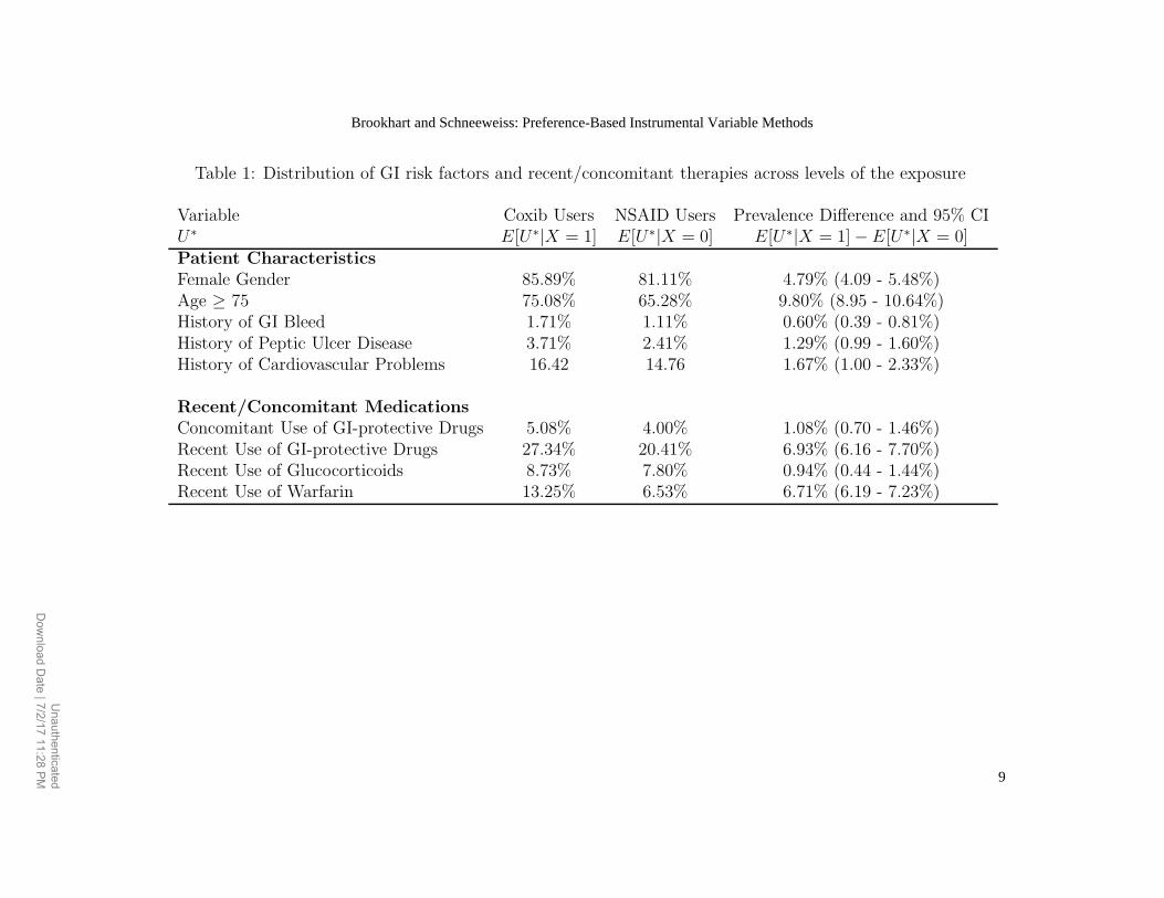
Table 1: Distribution of GI risk factors and recent/concomitant therapies across levels of the exposure

Variable Coxib Users NSAID Users Prevalence Difference and 95% CIU∗ E[U∗|X = 1] E[U∗|X = 0] E[U∗|X = 1] − E[U∗|X = 0]Patient CharacteristicsFemale Gender 85.89% 81.11% 4.79% (4.09 - 5.48%)Age ≥ 75 75.08% 65.28% 9.80% (8.95 - 10.64%)History of GI Bleed 1.71% 1.11% 0.60% (0.39 - 0.81%)History of Peptic Ulcer Disease 3.71% 2.41% 1.29% (0.99 - 1.60%)History of Cardiovascular Problems 16.42 14.76 1.67% (1.00 - 2.33%)

Recent/Concomitant MedicationsConcomitant Use of GI-protective Drugs 5.08% 4.00% 1.08% (0.70 - 1.46%)Recent Use of GI-protective Drugs 27.34% 20.41% 6.93% (6.16 - 7.70%)Recent Use of Glucocorticoids 8.73% 7.80% 0.94% (0.44 - 1.44%)Recent Use of Warfarin 13.25% 6.53% 6.71% (6.19 - 7.23%)

9


Unauthenticated

Dow

nload Date | 7/2/17 11:28 PM

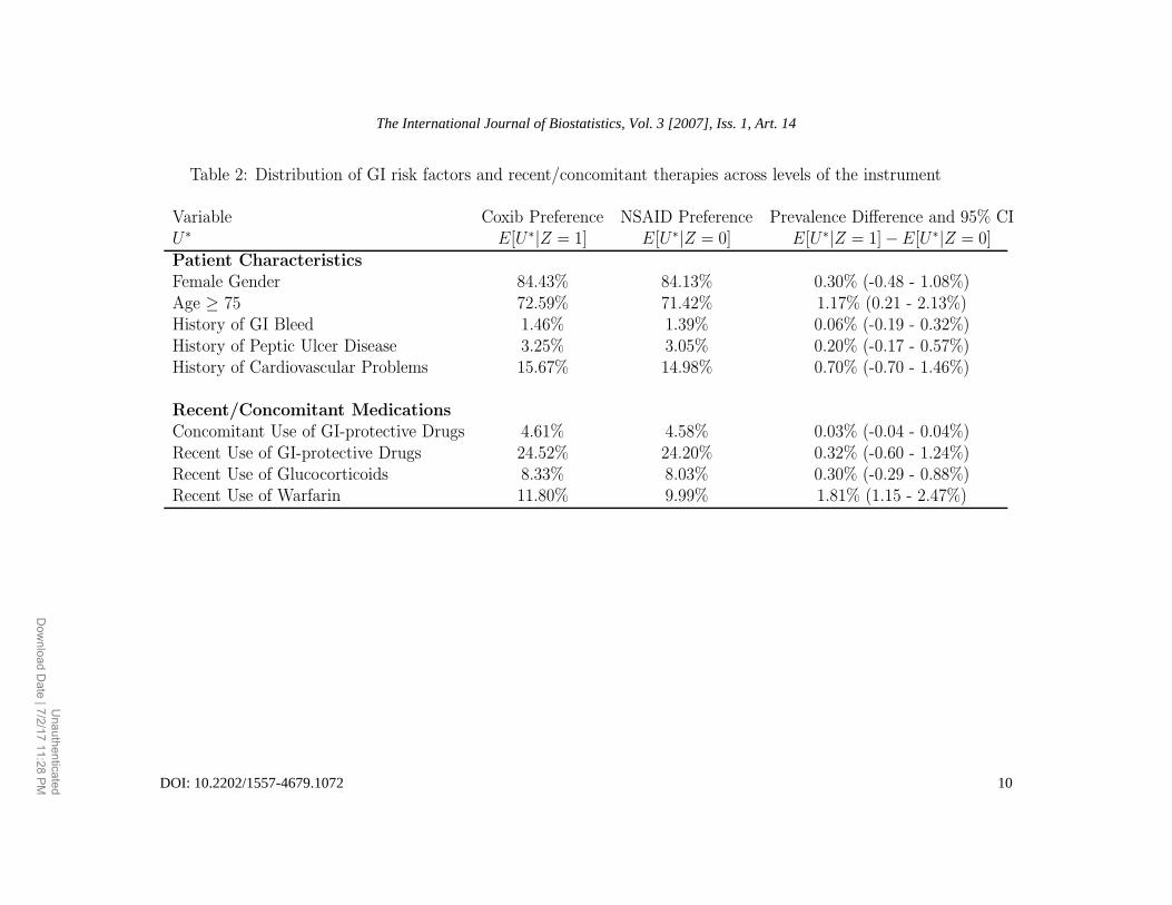
Table 2: Distribution of GI risk factors and recent/concomitant therapies across levels of the instrument

Variable Coxib Preference NSAID Preference Prevalence Difference and 95% CIU∗ E[U∗|Z = 1] E[U∗|Z = 0] E[U∗|Z = 1] − E[U∗|Z = 0]Patient CharacteristicsFemale Gender 84.43% 84.13% 0.30% (-0.48 - 1.08%)Age ≥ 75 72.59% 71.42% 1.17% (0.21 - 2.13%)History of GI Bleed 1.46% 1.39% 0.06% (-0.19 - 0.32%)History of Peptic Ulcer Disease 3.25% 3.05% 0.20% (-0.17 - 0.57%)History of Cardiovascular Problems 15.67% 14.98% 0.70% (-0.70 - 1.46%)

Recent/Concomitant MedicationsConcomitant Use of GI-protective Drugs 4.61% 4.58% 0.03% (-0.04 - 0.04%)Recent Use of GI-protective Drugs 24.52% 24.20% 0.32% (-0.60 - 1.24%)Recent Use of Glucocorticoids 8.33% 8.03% 0.30% (-0.29 - 0.88%)Recent Use of Warfarin 11.80% 9.99% 1.81% (1.15 - 2.47%)

10


DOI: 10.2202/1557-4679.1072

Unauthenticated

Dow

nload Date | 7/2/17 11:28 PM

ther bias in this estimator relative to the average effect of treatment in thepopulation?

In the following sections we consider how our sensitivity analysis frameworkmay illuminate these issues. To simplify exposition and to facilitate intuition,we consider two scenarios: one in which the exclusion restriction is violated,but the average effect of treatment does not vary with the unmeasured vari-able U ; and another in which the exclusion restriction holds, but the averagetreatment effect varies with U .

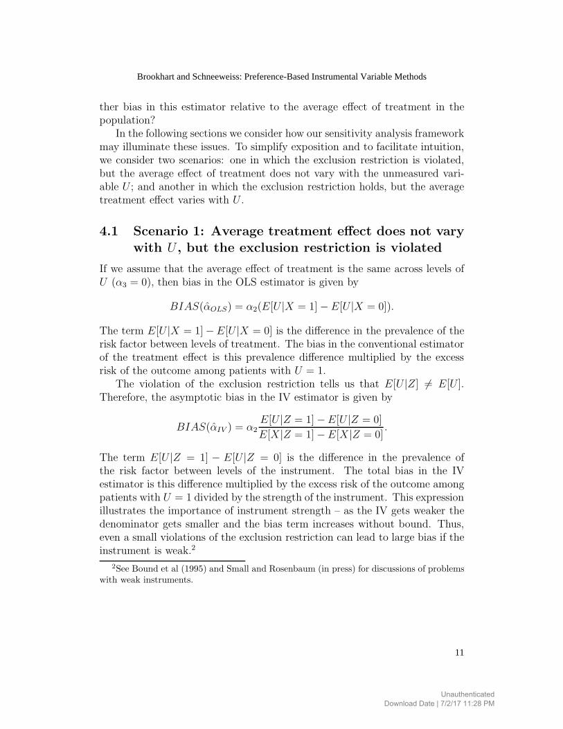
4.1 Scenario 1: Average treatment effect does not vary

with U , but the exclusion restriction is violated

If we assume that the average effect of treatment is the same across levels ofU (α3 = 0), then bias in the OLS estimator is given by

BIAS(αOLS) = α2(E[U |X = 1] − E[U |X = 0]).

The term E[U |X = 1] − E[U |X = 0] is the difference in the prevalence of therisk factor between levels of treatment. The bias in the conventional estimatorof the treatment effect is this prevalence difference multiplied by the excessrisk of the outcome among patients with U = 1.

The violation of the exclusion restriction tells us that E[U |Z] 6= E[U ].Therefore, the asymptotic bias in the IV estimator is given by

BIAS(αIV ) = α2E[U |Z = 1] − E[U |Z = 0]

E[X|Z = 1] − E[X|Z = 0].

The term E[U |Z = 1] − E[U |Z = 0] is the difference in the prevalence ofthe risk factor between levels of the instrument. The total bias in the IVestimator is this difference multiplied by the excess risk of the outcome amongpatients with U = 1 divided by the strength of the instrument. This expressionillustrates the importance of instrument strength – as the IV gets weaker thedenominator gets smaller and the bias term increases without bound. Thus,even a small violations of the exclusion restriction can lead to large bias if theinstrument is weak.2

2See Bound et al (1995) and Small and Rosenbaum (in press) for discussions of problemswith weak instruments.

11



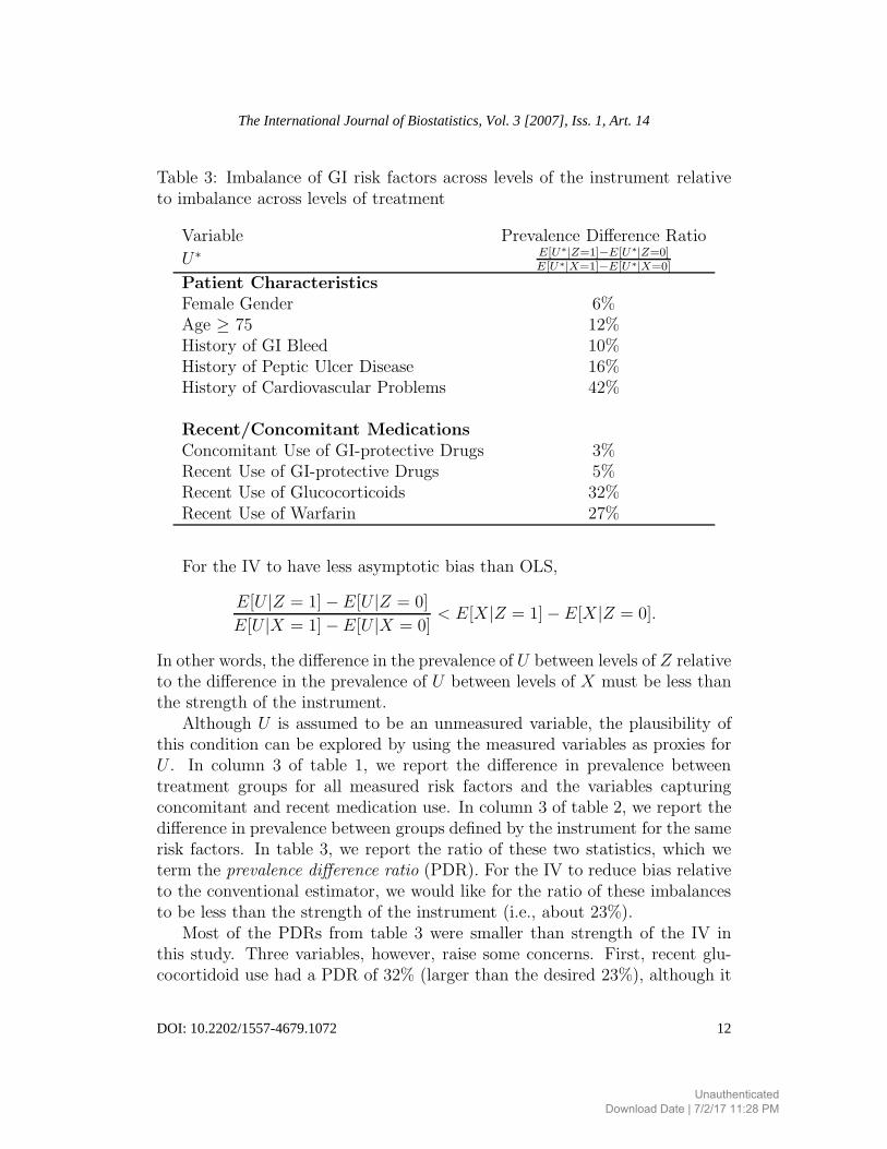
Table 3: Imbalance of GI risk factors across levels of the instrument relativeto imbalance across levels of treatment

Variable Prevalence Difference Ratio

U∗ E[U∗|Z=1]−E[U∗|Z=0]E[U∗|X=1]−E[U∗|X=0]

Patient CharacteristicsFemale Gender 6%Age ≥ 75 12%History of GI Bleed 10%History of Peptic Ulcer Disease 16%History of Cardiovascular Problems 42%

Recent/Concomitant MedicationsConcomitant Use of GI-protective Drugs 3%Recent Use of GI-protective Drugs 5%Recent Use of Glucocorticoids 32%Recent Use of Warfarin 27%

For the IV to have less asymptotic bias than OLS,

E[U |Z = 1] − E[U |Z = 0]

E[U |X = 1] − E[U |X = 0]< E[X|Z = 1] − E[X|Z = 0].

In other words, the difference in the prevalence of U between levels of Z relativeto the difference in the prevalence of U between levels of X must be less thanthe strength of the instrument.

Although U is assumed to be an unmeasured variable, the plausibility ofthis condition can be explored by using the measured variables as proxies forU . In column 3 of table 1, we report the difference in prevalence betweentreatment groups for all measured risk factors and the variables capturingconcomitant and recent medication use. In column 3 of table 2, we report thedifference in prevalence between groups defined by the instrument for the samerisk factors. In table 3, we report the ratio of these two statistics, which weterm the prevalence difference ratio (PDR). For the IV to reduce bias relativeto the conventional estimator, we would like for the ratio of these imbalancesto be less than the strength of the instrument (i.e., about 23%).

Most of the PDRs from table 3 were smaller than strength of the IV inthis study. Three variables, however, raise some concerns. First, recent glu-cocortidoid use had a PDR of 32% (larger than the desired 23%), although it

12


DOI: 10.2202/1557-4679.1072


was not significantly associated with the IV. Secondly, recent use of warfarinhad a statistically significantly association with the instrument and its PDRwas 27% (also slightly more than the desired 23%). Finally, the PDR associ-ated with a history of cardiovascular problems was 56%, although it was notsignificantly associated with the instrument.3

Instrumental variable methods can make statistical adjustments for thesepotentially problematic measured covariates; however, the residual associa-tions between the instrument and several observed variables raise the possi-bility of associations between the instrument and important unmeasured vari-ables. In particular, the associations between the instrument and two differenttreatment modalities (warfarin and glucocorticoids) suggest that physicianswho frequently prescribe coxibs practice differently from physicians who pre-fer to prescribe non-selective NSAIDs. Fortunately, there are relatively fewactions that a physician could take to alter a patient’s short-term GI risk andthose can be measured well in health care utilization data. For example, wecan take account of all medications that a patient might use that could affectGI risk. In studies of all-cause mortality, strong residual associations betweenthe IV and other treatment modalities would be more concerning as there maybe many ways physicians affect mortality risk.4

As expected, we found that coxib exposure was positively associated withGI risk factors. To the extent that exposure has a similar association withunmeasured GI risk factors, confounding bias would cause the conventionalanalysis to underestimate the average effect of coxib treatment in the popu-lation. Similarly, we found that the IV had a weak positive association withsome GI risk factors. To the extent that the IV has a similar association withunmeasured GI risk factors, violations of the exclusion restriction would havecaused the IV estimator to underestimate the average effect of coxib treatmentin the population. We found, however, that the PDR for most variables, par-ticularly patient characteristics strongly related to GI risk, was less than 23%;therefore we think that the degree of underestimation in the IV approach islikely to be smaller than in the conventional analysis.

3A history of cardiovascular problems is not clearly a GI risk factor, but it may becorrelated with other GI risk factors such as obesity and smoking status.

4See Ray (2006) for a discussion of the increased potential for confounding in studies ofall-cause mortality.

13



4.2 Scenario 2: Exclusion restriction holds, but averagetreatment effect varies with U

In this section, we assume that the exclusion restriction holds, so E[U |Z =1] − E[U |Z = 0] = 0, but the average treatment effect varies with U , so thatα3 6= 0. Here we imagine U to be an unmeasured patient risk factor that is asource of treatment effect heterogeneity.

Under these assumptions, the asymptotic bias in the IV estimator is givenby

BIAS(αIV ) = α3E[U ]

[

E[X|Z = 1, U = 1] − E[X|Z = 0, U = 1]

E[X|Z = 1] − E[X|Z = 0]− 1

]

. (6)

The denominator is the strength of the instrument in the population. Thenumerator is the strength of the instrument among people with U = 1, e.g.,those with a particular unmeasured GI risk factor. From this expression wecan make two immediate observations. First, if the strength of the instrumentis the same in both groups defined by U , then the bias is zero. Second, ifthe instrument is not predictive of exposure among patients with U = 1,i.e., E[X|Z = 1, U = 1] − E[X|Z = 0, U = 1] = 0, then the bias is equalto −α3E[U ]. Thus, the IV estimates the average effect of treatment amongpeople with U = 0. This would be the case if a patient with the risk factorwere equally likely to be treated by either type of physician. One extremeexample of this would be patients who are always treated or never treated.

Next we consider how subject-matter knowledge of medical practice pat-terns can be used to anticipate the magnitude and direction of this bias term.

4.2.1 Bias in the IV estimator when medications or procedures areoverused in the population under study

During the period of our study, coxibs were thought to be generally overused,more likely to be prescribed to patients who did not need them than to bewithheld from patients who needed them (Desmet et al, 2006). Let U denotean unmeasured GI risk factor (e.g., smoking status) that is observed by thephysician and could modify the effect of coxib exposure. If coxibs are overused,then patients who have an indication for a coxib are likely to get a coxib fromeither type of physician. The additional people being treated by physicianswith Z = 1 are those who are less likely to benefit from a coxib. In thisscenario, 0 ≤ E[X|Z = 1, U = 1] − E[X|Z = 0, U = 1] < E[X|Z = 1] −

14


DOI: 10.2202/1557-4679.1072


E[X|Z = 0]. If α3 < 0, the bias is bounded as follows

0 < BIAS(αIV ) ≤ −α3E[U ].

Here the IV estimator is over-weighting the effect of treatment in the low-riskgroup.

To better understand this bias, consider the extreme example in whichall patients who could benefit from a coxib would get one regardless of thephysician’s preference. In this case, Z will have no marginal association withthe outcome (E[Y |Z = 1] − E[Y |Z = 0] = 0), and the IV estimand will bezero. The IV is reflecting the effect of treatment in a population of patientswho would not benefit from treatment with coxibs and thus underestimatesthe average effect of coxib exposure in the larger population.

4.2.2 Bias in the IV when medications or procedures are underusedin the population under study

In many cases, medications and medical procedures are thought to be un-derused, in that they are not given to many patients who might benefit fromthem. One well-known example is bone resorption agents that are used to treatosteoporosis (Solomon et al, 2003b). If these medications are underused, wewould expect the instrument to be more strongly related to treatment amongthose with clinically evident osteoporosis (e.g., low bone mineral density testresults, history of osteoporotic fractures) than among an entire population ofolder women. If U indicates a risk factor for a fracture, we anticipate thatE[X|Z = 1, U = 1] − E[X|Z = 0, U = 1] > E[X|Z = 1] − E[X|Z = 0].If α3 < 0, then BIAS(αIV ) < 0. Here, the IV estimator is extrapolatingthe treatment effect of bone resorption agents in a high-risk group to the en-tire population. If treatment is more effective in high-risk patients and theinstrument is also stronger within this group, treatment effect heterogeneitywould lead preference-based IV estimators to exaggerate the protective effectof medications or procedures at the population level.

4.2.3 Bias in the IV estimator when medications or procedures aremisused in the population under study

In some cases, medications or medical procedures may be misused, in thesense that they may be given to patients with specific contraindications, ornecessary follow-up tests are not performed after patients have been startedon a medication. Preference-based IV studies of drugs or procedures that arecommonly misused can be subject to counter-intuitive biases.

15



For example, consider a study that compares the safety of metformin toother oral antihyperglycemic drugs used to treat Type II diabetes. Metforminis contraindicated in patients with decreased renal function or liver disease, asit can cause lactic acidosis, a potentially fatal side effect. We speculate thatphysicians who infrequently use metformin will be less likely to understand itscontraindications and therefore would be more likely to misuse it. Let U be anindicator of decreased renal function or liver disease. If our hypothesis is true,then E[X|Z = 1, U = 1]−E[X|Z = 0, U = 1] < 0. In other words, physicianswith Z = 1 are less likely than physicians with Z = 0 to prescribe metforminto patients with a contraindication. In this case, a preference-based IV couldmake metformin appear to prevent lactic acidosis, as patients of physicianswith Z = 1 are at lower risk of being inappropriately treated.

4.2.4 Empirically evaluating the magnitude and direction of biasdue to treatment effect heterogeneity

The results from this section suggest that we can look for evidence of bias dueto treatment effect heterogeneity using observed data. The expression (6) forthe bias depends on the strength of the instrument within the sub-populationdefined by U = 1 relative to the strength of the instrument in the entirepopulation. Because U is a variable that is assumed to be unobserved, wepropose to use measured factors as proxies for U . If the strength of the instru-ment varies strongly across different sub-groups defined by observed factors,we would anticipate that instrument strength is likely to vary across subgroupsdefined by unobserved variables leading the IV estimator to be inconsistentfor the average effect of treatment in the population.

For example, we have speculated that, consistent with other research, cox-ibs are likely to be overused in our study population (Desmet et al, 2006). Toevaluate this assertion, we examined whether the strength of the instrument inthe population was different from the strength of the instrument within spe-cific subgroups. If coxibs are overused, we would expect the IV to be weakerwithin subgroups defined by strong GI risk factors.

Table 4 presents the strength of the instrument within sub-groups definedby measured variables. We observed that the IV was slightly weaker withinstrata of the strongest GI risk factors. However, in only one sub-group did thedifference in instrument strength reach statistical significance (among recentusers of warfarin). To the extent that coxib exposure is more effective (on arisk difference scale) in high risk patients, treatment effect heterogeneity mayhave caused our IV estimand to slightly understate the average protectiveeffect of coxib exposure in our population.

16


DOI: 10.2202/1557-4679.1072


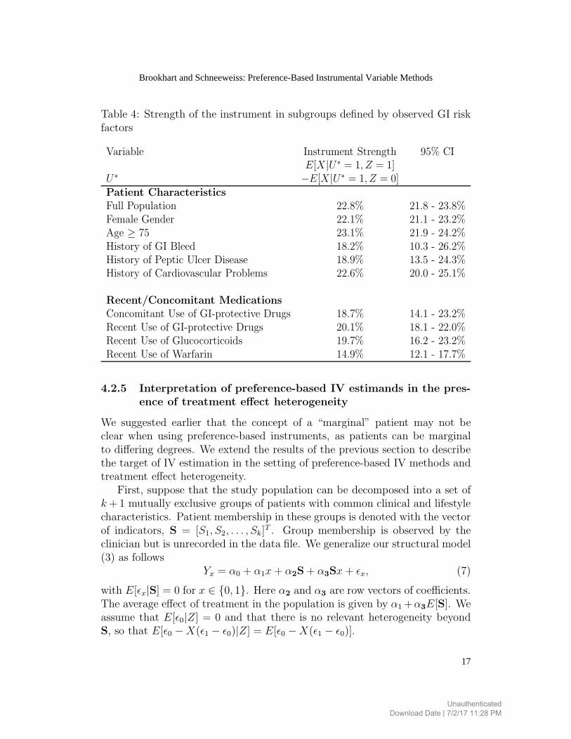
Table 4: Strength of the instrument in subgroups defined by observed GI riskfactors

Variable Instrument Strength 95% CIE[X|U∗ = 1, Z = 1]

U∗ −E[X|U∗ = 1, Z = 0]Patient CharacteristicsFull Population 22.8% 21.8 - 23.8%Female Gender 22.1% 21.1 - 23.2%Age ≥ 75 23.1% 21.9 - 24.2%History of GI Bleed 18.2% 10.3 - 26.2%History of Peptic Ulcer Disease 18.9% 13.5 - 24.3%History of Cardiovascular Problems 22.6% 20.0 - 25.1%

Recent/Concomitant MedicationsConcomitant Use of GI-protective Drugs 18.7% 14.1 - 23.2%Recent Use of GI-protective Drugs 20.1% 18.1 - 22.0%Recent Use of Glucocorticoids 19.7% 16.2 - 23.2%Recent Use of Warfarin 14.9% 12.1 - 17.7%

4.2.5 Interpretation of preference-based IV estimands in the pres-ence of treatment effect heterogeneity

We suggested earlier that the concept of a “marginal” patient may not beclear when using preference-based instruments, as patients can be marginalto differing degrees. We extend the results of the previous section to describethe target of IV estimation in the setting of preference-based IV methods andtreatment effect heterogeneity.

First, suppose that the study population can be decomposed into a set ofk + 1 mutually exclusive groups of patients with common clinical and lifestylecharacteristics. Patient membership in these groups is denoted with the vectorof indicators, S = [S1, S2, . . . , Sk]

T . Group membership is observed by theclinician but is unrecorded in the data file. We generalize our structural model(3) as follows

Yx = α0 + α1x + α2S + α3Sx + ǫx, (7)

with E[ǫx|S] = 0 for x ∈ {0, 1}. Here α2 and α3 are row vectors of coefficients.The average effect of treatment in the population is given by α1 +α3E[S]. Weassume that E[ǫ0|Z] = 0 and that there is no relevant heterogeneity beyondS, so that E[ǫ0 − X(ǫ1 − ǫ0)|Z] = E[ǫ0 − X(ǫ1 − ǫ0)].

17



Assuming that E[S|Z] = E[S], we can extend the results from the previoussection to show that

E[Y |Z = 1] − E[Y |Z = 0]

E[X|Z = 1] − E[X|Z = 0]= α1 +

k∑

j=1

α3,jE[Sj ]wj.

The estimated treatment effect turns out to be a “weighted average” of treat-ment effects in different sub-groups, where the weights are given by

wj =

[

E[X|Z = 1, Sj = 1] − E[X|Z = 0, Sj = 1]

E[X|Z = 1] − E[X|Z = 0]

]

,

and thus could be negative or have absolute values greater than one.The interpretation of the weights follows from the previous discussion of

treatment effect heterogeneity. If the instrument is stronger in sub-group j

than in the population, then the sub-group weight is greater than one andthe effect of treatment in that sub-group is up-weighted. If the instrumentis weaker in sub-group j than in the population, the sub-group weight is lessthan one and the effect of treatment in that sub-group is down-weighted. Ifthe effect of the instrument is reversed in sub-group j, e.g., in the case ofcontraindications, the weight will be negative. Lastly, if the IV does notpredict treatment in a particular group, than the weight is zero and the effectof treatment in that sub-group is not reflected in the IV estimand.

For example, consider the case of statins, cholesterol-lowering drugs thatare thought to be substantially underused, in that they are not given to manypatients who might benefit from them (Majumdar et al, 1999). Suppose weare doing a typical study using health care claims data to assess the effec-tiveness of statins in a population at-risk of an acute coronary event. Usinghealth care claims data, we attempt to identify a study population consistingof people with at least one cardiovascular risk factor, e.g., patients with a di-agnosis of hypertension, unstable angina, myocardial infarction, diabetes, orhypercholesterolemia. In this population there is still considerable variationin underlying risk. We speculate that those at greatest risk, e.g., those whosmoke, are overweight, and who have a history of myocardial infarction, willbe treated with statins by many physicians. Therefore the contribution of thetreatment effects in the highest-risk group could be down-weighted. Similarly,those at lowest risk may be treated by few physicians of either type, and theircontribution to the IV estimate would also be down-weighted. The instrumentmay be the strongest among patients at moderate risk, so the IV estimate maytend to reflect the effect of treatment in these patients. In the case of statins,

18


DOI: 10.2202/1557-4679.1072


which are relatively safe with few contraindications, there are not likely to bepathologies that would lead a small sub-group to have a very large negativeweight.

Finally, we note that one can explore the likely magnitude and directionsof these weights empirically. As we proposed earlier, by assessing the strengthof the instrument within sub-groups, researchers can gather evidence aboutimportant differences in practice patterns between physicians with Z = 1 andthose with Z = 0. For example, to explore the plausibility of our hypothesisabout statin prescribing, we could examine the strength of the IV across arange of sub-groups of varying degrees of cardiovascular risk according to theobserved variables.

5 Discussion

We have discussed issues related to the validity and interpretation of studiesusing preference-based instrumental variables that are defined at the level of ahealth care provider or an aggregation of providers. We have illustrated variousways that observed variables can be used as proxies for unobserved confoundersto anticipate the direction of bias due to violations of IV assumptions. Usingthese variables, we provided a benchmark to assess whether the IV approachis likely to reduce confounding bias relative to a conventional estimator oftreatment effect. We have also described how one can use observed variablesand subject matter knowledge to anticipate the direction of bias in a standardIV estimator due to treatment effect heterogeneity.

The ideas discussed in this paper were presented in the context of a studyof the short-term risk of GI bleeding among elderly new users of non-selective,non-steroidal anti-inflammatory drugs. The analysis based on the methodsdescribed herein suggested that, in the absence of treatment effect heterogene-ity, violations of the exclusion restriction may have caused our IV estimate toslightly underestimate the average effect of coxib treatment in the population.This is due primarily to the IV having a weak positive association with someGI risk factors and recent use of medications that can increase GI risk. Tothe extent the measured variables are reasonable proxies for the unmeasuredvariables, our analysis suggested that the bias in the IV is likely to be smallerthan the bias in a conventional analysis.

We also found that treatment effect heterogeneity may have led to a modestdifference between the IV estimand and the average treatment effect in thepopulation. Empirical data suggest that patients at lower GI risk were slightlymore likely to have had their treatment influenced by the IV. According to the

19



framework we have described, the contribution of the effect of treatment inthese patients may be slightly up-weighted by the IV estimator. To extent thatcoxibs may be less effective (on a risk difference scale) in lower-risk patients,treatment effect heterogeneity would have caused the IV estimator to furtherunderstate the average protective effect of coxibs in the population.

In the expressions for bias that we have derived, it is assumed that the pa-rameter of interest is the average effect of treatment in the population understudy. This parameter is of inherent interest as it is what would be estimatedby an RCT conducted in the population. However, in many observational stud-ies of drugs and medical procedures, the population under study may includemany patients for whom there is little clinical equipoise (i.e., patients whowould be rarely or almost always treated). In these settings, other measuresof treatment effect may be of greater interest. For example, when many pa-tients are appropriately untreated, one may be more interested in the averageeffect of treatment on those who received treatment (the effect of treatmenton the treated). When drugs are underused in the population under study,and the IV affects treatment in a small, high-risk segment of the population,the IV estimand is likely to be closer to the average effect of treatment in thetreated than the average effect of treatment in the population.

Our study is limited by the simplicity of our analytic framework. We haveconsidered bias in a standard IV estimator with a single dichotomous instru-ment, unmeasured covariate, and treatment. For more complex situationsinvolving non-linear models, continuous treatments, and multiple continuousinstruments, the analyst will need to use subject-matter expertise to make as-sumptions about both the model for the treatment choice and outcome. Whentreatment effects are heterogeneous, the interpretation of the effect estimatecan depend on the assumptions one makes about these models. Our resultswill not immediately apply to these more complex settings.

As with any analysis of observational data, studies using preference-basedIV methods rely on assumptions that cannot be verified with observed data.In many cases, these assumptions will not completely hold, and IV methodsmay lead to estimates that are both highly biased and excessively variable. Wehave outlined an approach that can be used to assess the likely extent of theproblem. Further research may reveal additional ways to evaluate the validityof preference-based IV methods or to improve them through study design orstatistical innovations.

20


DOI: 10.2202/1557-4679.1072


References

[1] Walker A. Confounding by indication. Epidemiology 1996; 7(4): 335-6.

[2] Angrist J, Imbens G, Rubin DB. Identification of causal effects using in-strumental variable. J Amer Stat Assoc. 1996; 91(434): 444-455.

[3] Greenland S. An introduction to instrumental variables for epidemiologists.Int J Epidemiol. 2000; 29: 722-729.

[4] Martens EP, Pestman WR, de Boer A, Belitser SV, Klungel OH. Instru-mental variables: application and limitations. Epidemiology. 2006; 17(3):260-7.

[5] Hernan MA, Robins JM. Instruments for causal inference: an epidemiolo-gist’s dream? Epidemiology. 2006; 17(4): 360-72.

[6] Wen SW, Kramer MS. Uses of ecologic studies in the assessment of intendedtreatment effects. J Clin Epidemiol. 1999; 52(1): 7-12.

[7] Brooks JM, Chrischilles EA, Scott SD, Chen-Hardee SS. Was breast con-serving surgery underutilized for early stage breast cancer? Instrumentalvariables evidence for stage II patients from Iowa. Health Serv Res. 2003;38(6 Pt 1): 1385-402.

[8] Stukel TA, Fisher ES, Wennberg DE, Alter DA, Gottlieb DJ, VermeulenMJ. Analysis of observational studies in the presence of treatment selec-tion bias: effects of invasive cardiac management on AMI survival usingpropensity score and instrumental variable methods. JAMA. 2007; 297(3):278-85.

[9] Johnston SC. Combining ecological and individual variables to reduce con-founding by indication: case study–subarachnoid hemorrhage treatment. JClin Epidemiol. 2000; 53(12): 1236-41

[10] Brookhart MA. Assessing the safety of recombinant erythropoietin usinginstrumental variable methods [abstract]. Meeting of the International Bio-metrics Society, Eastern North American Region, Atlanta, Georgia, 2007.

[11] Korn MA, Baumrind E. Clinician preferences and the estimation of causaltreatment differences. Statistical Science. 1998; 13(3): 209-35.

21



[12] Brookhart MA, Wang PS, Solomon DH, Schneeweiss S. Evaluating short-term drug effects using a physician-specific prescribing preference as aninstrumental variable. Epidemiology. 2006; 17(3): 268-75.

[13] Wang PS, Schneeweiss S, Avorn J, Fischer MA, Mogun H, Solomon DH,Brookhart MA. Risk of death in elderly users of conventional vs. atypicalantipsychotic medications. N Engl J Med. 2005; 353(22): 2335-41.

[14] Laporte JR, Ibanez L, Vidal X, Vendrell L, Leone R. Upper gastrointesti-nal bleeding associated with the use of NSAIDs: newer versus older agents.Drug Saf. 2004; 27(6): 411-20.

[15] Solomon DH, Schneeweiss S, Glynn RJ, Levin R, Avorn J. Determinantsof selective cyclooxygenase-2 inhibitor prescribing: are patient or physiciancharacteristics more important? Am J Med. 2003; 115(9): 715-20.

[16] Schneeweiss S, Glynn RJ, Avorn J, Solomon DH. A Medicare databasereview found that physician preferences increasingly outweighed patientcharacteristics as determinants of first-time prescriptions for COX-2 in-hibitors. J Clin Epidemiol. 2005; 58(1): 98-102.

[17] Brookhart MA, Polinski JM, Avorn J, Mogun H, Solomon DH. The medi-cal license number accurately identifies the prescribing physician in a largepharmacy claims dataset. Med Care. 2007; 45(9): 907-910.

[18] Rubin DB. Estimating causal effects of treatment in randomized and non-randomized studies. Journal of Eductional Psychology. 1974; 66: 688-701.

[19] Rubin DB. Statistics and causal inference. Comment: which ifs havecausal answers? J Amer Stat Assoc. 1986; 81: 961-962.

[20] Imbens G, Angrist J. Identification and estimation of local average treat-ment effects. Econometrica. 1994; 62 (2): 467-476.

[21] Harris KM. Remler DK. Who is the marginal patient? Understanding in-strumental variables estimates of treatment effects. Health Serv Res. 1998;33(5 Pt 1): 1337-60.

[22] Wooldridge J. On two-stage least squares estimation of the average treat-ment effect in a random coefficient model. Economic Letters. 1997; 56:129133

[23] Heckman JJ, Urzua S, Vytlacil EJ. Understanding instrumental variablemodels with essential heterogeneity. NBER working paper, 12574, 2006.

22


DOI: 10.2202/1557-4679.1072


[24] Bound J, Jaeger DA, Baker RM. Problems with instrumental variablesestimation when the correlation between the instruments and the endoge-nous explanatory variable is weak. J Am Stat Assoc. 1995; 90: 443-450.

[25] Small D, Rosenbaum PR. War and Wages: The strength of instrumentalvariables and their sensitivity to unobserved biases. J Am Stat Assoc. Inpress.

[26] Ray WA. Observational studies of drugs and mortality. N Engl J Med.2005; 353(22): 2319-2321.

[27] De Smet BD, Fendrick MA,Stevenson JG, Bernstein SJ. Over and Under-utilization of cyclooxygenase-2 selective inhibitors by primary care physi-cians and specialists: the tortoise and the hare revisited. J Gen Intern Med.2006; 21: 694-697.

[28] Solomon DH, Finkelstein JS, Katz JN, Mogun H, Avorn J. Underuse ofosteoporosis medications in elderly patients with fractures. Am J Med.2003(b); 115(5): 398-400.

[29] Majumdar SR, Gurwitz JH, Soumerai SB. Undertreatment of hyperlipi-demia in the secondary prevention of coronary artery disease. J Gen InternMed. 1999; 14: 711-717.

23



Documents

The International Journal of Biostatistics - Semantic … International Journal of Biostatistics ... Results M. Alan Brookhart, Division of Pharmacoepidemiology, Brigham and Women's