The International Journal of 3D LIDAR–camera intrinsic andstergios/papers/IJRR-2012... · 454 The International Journal of Robotics Research 31(4) Side View Top View i - th laser

3D LIDAR–camera intrinsic andextrinsic calibration: Identifiability andanalytical least-squares-basedinitialization

The International Journal ofRobotics Research31(4) 452–467© The Author(s) 2012Reprints and permission:sagepub.co.uk/journalsPermissions.navDOI: 10.1177/0278364911435689ijr.sagepub.com

Faraz M Mirzaei, Dimitrios G Kottas and Stergios I Roumeliotis

AbstractIn this paper we address the problem of estimating the intrinsic parameters of a 3D LIDAR while at the same time com-puting its extrinsic calibration with respect to a rigidly connected camera. Existing approaches to solve this nonlinearestimation problem are based on iterative minimization of nonlinear cost functions. In such cases, the accuracy of theresulting solution hinges on the availability of a precise initial estimate, which is often not available. In order to addressthis issue, we divide the problem into two least-squares sub-problems, and analytically solve each one to determine a pre-cise initial estimate for the unknown parameters. We further increase the accuracy of these initial estimates by iterativelyminimizing a batch nonlinear least-squares cost function. In addition, we provide the minimal identifiability conditions,under which it is possible to accurately estimate the unknown parameters. Experimental results consisting of photorealistic3D reconstruction of indoor and outdoor scenes, as well as standard metrics of the calibration errors, are used to assessthe validity of our approach.

KeywordsSensing and perception, computer vision, range sensing, calibration and identification

1. Introduction

As demonstrated in the Defense Advanced ResearchProjects Agency (DARPA) Urban Challenge, commerciallyavailable high-speed 3D LIDARs, such as the Velodyne,have made autonomous navigation and mapping withindynamic environments possible. In most applications, how-ever, another sensor is employed in conjunction with the3D LIDAR to assist in localization and place recognition.In particular, spherical cameras are often used to providevisual cues and to construct photorealistic maps of the envi-ronment. In these scenarios, accurate extrinsic calibration ofthe six degrees of freedom (d.o.f.) transformation betweenthe two sensors is a prerequisite for optimally combiningtheir measurements.

Several methods exist for calibrating a 2D laser scannerwith respect to a camera. The work of Zhang and Pless(2004) relies on the observation of a planar checkerboardby both sensors. In particular, corners are detected in theimages and planar surfaces are extracted from the lasermeasurements. The detected corners are used to determinethe normal vector and distance of the planes where thelaser-scan endpoints lie. Using this geometric constraint,the estimation of the transformation between the two sen-sors is formulated as a nonlinear least-squares problem andsolved iteratively. A simplified linear least-squares solution

is also provided to initialize the iterative nonlinear algo-rithm. More recently, Naroditsky et al. (2011) have pre-sented a minimal approach for calibrating a 2D laser scan-ner with respect to a camera, using only six measurementsof a planar calibration board. The computed transformationis then used in conjunction with RAndom Sample Consen-sus (RANSAC) (Fischler and Bolles 1981) to initialize aniterative least-squares refinement.

The existing 2D laser scanner–camera calibration meth-ods have been extended to 3D LIDARs by Unnikrishnanand Hebert (2005) and Pandey et al. (2010). In both works, ageometric constraint similar to that presented by Zhang andPless (2004) is employed to form a nonlinear least-squarescost function which is iteratively minimized to estimatethe LIDAR–camera transformation. In addition, Unnikr-ishnan and Hebert (2005) have presented an initializationmethod for the iterative minimization based on a simplified

Department of Computer Science and Engineering, University ofMinnesota, Minneapolis, MN, USA

Corresponding author:Faraz M Mirzaei, Department of Computer Science and Engineering,University of Minnesota, 4-192 Keller Hall, 200 Union Street SE, Min-neapolis, MN 55455, USA.Email: [email protected]

at Serials Records, University of Minnesota Libraries on September 4, 2012ijr.sagepub.comDownloaded from

http://ijr.sagepub.com/

Mirzaei et al. 453

linear least-squares formulation. Specifically, the estima-tion of relative rotation and translation are decoupled, andthen each of them is computed from a geometric constraintbetween the planar segments detected in the measurementsof both the 3D LIDAR and the camera. An alternative3D LIDAR–camera calibration approach is described byScaramuzza et al. (2007), where several point correspon-dences are manually selected in images and their associatedLIDAR scans. Then, the Perspective n-point Pose (PnP)estimation algorithm of Quan and Lan (1999) is employedto find the transformation between the camera and the 3DLIDAR based on these point correspondences. In a differentapproach, presented by Stamos et al. (2008), the structuraledges extracted from 3D LIDAR scans are matched with thevanishing points of the corresponding 2D images to com-pute a coarse 3D LIDAR–camera transformation, followedby an iterative least-squares refinement.

The main limitation of the above methods is that theyassume the 3D LIDAR to be intrinsically calibrated. Ifthe LIDAR’s intrinsic calibration is not available or suffi-ciently accurate, then the calibration accuracy as well asthe performance of subsequent LIDAR–camera data fusionsignificantly degrades. Pandey et al. (2010) have partiallyaddressed this issue for the Velodyne 3D LIDAR by firstcalibrating only some of its intrinsic parameters. However,the suggested intrinsic calibration procedure is also itera-tive, and no method is provided for initializing it. Whileseveral of the intrinsic parameters of a LIDAR may be ini-tialized using the technical drawings of the device (if avail-able), other parameters, such as the offset in the range mea-surements induced by the delay in the electronic circuits,cannot be determined in this way.

To address these limitations, in this work we propose anovel algorithm for jointly estimating the intrinsic parame-ters of a revolving-head 3D LIDAR as well as the LIDAR–camera transformation. Specifically, we use measurementsof a calibration plane at various configurations to estab-lish geometric constraints between the LIDAR’s intrinsicparameters and the LIDAR–camera 6 d.o.f. relative trans-formation. We process these measurement constraints toestimate the calibration parameters as follows: First, weanalytically compute an initial estimate for the intrinsicand extrinsic calibration parameters in two steps. Sub-sequently, we employ a batch iterative (nonlinear) least-squares method to refine the accuracy of the estimatedparameters.

In particular, to analytically compute an initial estimate,we relax the estimation problem by seeking to determinethe transformation between the camera and each one ofthe conic laser scanners within the LIDAR, along with itsintrinsic parameters. As a first step, we formulate a nonlin-ear least-squares problem to estimate the 3 d.o.f. rotationbetween each conic laser scanner and the camera, as wellas a subset of the laser scanner’s intrinsic parameters. Theoptimality conditions of this nonlinear least-squares prob-lem form a system of polynomial equations, which we solve

analytically using an algebraic-geometry approach to findall of its critical points. Amongst these, the one that min-imizes the least-squares cost function corresponds to theglobal minimum and provides us with the initial estimatesfor the relative rotation and the first set of intrinsic LIDARparameters. In the next step, we use a linear least-squaresalgorithm to compute the initial estimate for the relativetranslation between the camera and the conic laser scanners,and the remaining intrinsic parameters.

Once all initial estimates are available, we finally performa batch iterative joint optimization of the LIDAR–cameratransformation and the LIDAR’s intrinsic parameters. Aspart of our contributions, we also study the identifiabil-ity properties of the problem and present the minimalnecessary conditions for concurrently estimating theLIDAR’s intrinsic parameters and the LIDAR–cameratransformation. Our experimental results demonstrate thatour proposed method significantly improves the accuracyof the intrinsic calibration parameters of the LIDAR, aswell as the LIDAR–camera transformation.

The remainder of this paper is structured as follows.The calibration problem is formulated in Section 2, andthe proposed solution is presented in Section 3. In Section4 the identifiability of the problem is investigated and inSection 5, an experimental comparison of our method withthe approach of Pandey et al. (2010) is provided, and pho-torealistic 3D reconstruction of indoor and outdoor scenesusing the estimated calibration parameters are presented.Finally, in Section 6, the conclusions of this work are drawn,and suggestions for future research directions are provided.

2. Problem formulation

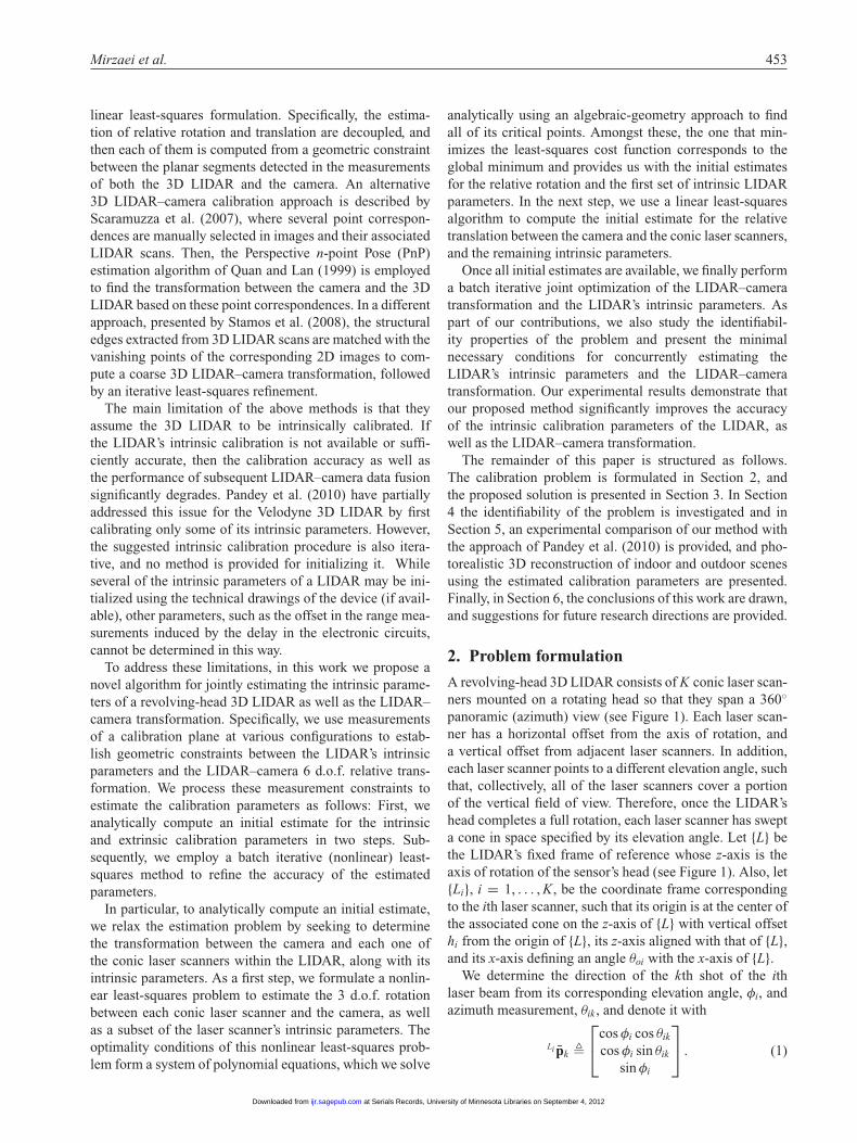
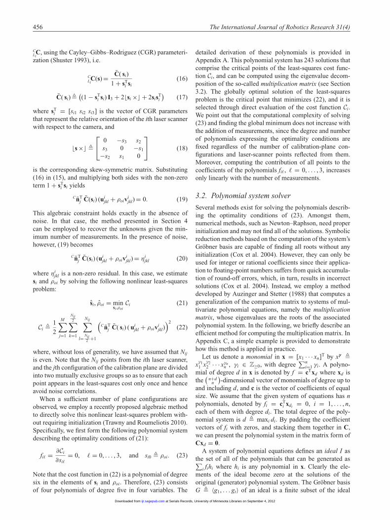
A revolving-head 3D LIDAR consists of K conic laser scan-ners mounted on a rotating head so that they span a 360◦

panoramic (azimuth) view (see Figure 1). Each laser scan-ner has a horizontal offset from the axis of rotation, anda vertical offset from adjacent laser scanners. In addition,each laser scanner points to a different elevation angle, suchthat, collectively, all of the laser scanners cover a portionof the vertical field of view. Therefore, once the LIDAR’shead completes a full rotation, each laser scanner has swepta cone in space specified by its elevation angle. Let {L} bethe LIDAR’s fixed frame of reference whose z-axis is theaxis of rotation of the sensor’s head (see Figure 1). Also, let{Li}, i = 1, . . . , K, be the coordinate frame correspondingto the ith laser scanner, such that its origin is at the center ofthe associated cone on the z-axis of {L} with vertical offsethi from the origin of {L}, its z-axis aligned with that of {L},and its x-axis defining an angle θoi with the x-axis of {L}.

We determine the direction of the kth shot of the ithlaser beam from its corresponding elevation angle, φi, andazimuth measurement, θik , and denote it with

Li pk �

⎡⎣cos φi cos θik

cos φi sin θik

sin φi

⎤⎦ . (1)



454 The International Journal of Robotics Research 31(4)

��

Top ViewSide View

i - th laserscanner

i - th laserscanner

Fig. 1. A revolving-head 3D LIDAR consists of K laser scan-ners, pointing to different elevation angles, and rotating arounda common axis. The intrinsic parameters of the LIDAR describethe measurements of each laser scanner in its coordinate frame,{Li}, and the transformation between the LIDAR’s fixed coordi-nate frame, {L}, and {Li}. Note that besides the physical offset ofthe laser scanners from the axis of rotation, the value of ρoi maydepend on the delay in the electronic circuits of the LIDAR.

The distance measured by the kth shot of the ith laser scan-ner is represented by ρik . The real distance to the object thatreflects the kth shot of the ith laser beam is αi(ρik + ρoi),where αi is the scale factor, and ρoi is the range offset dueto the delay in the electronic circuits of the LIDAR and theoffset of each laser scanner from its cone’s center. In thisway, the position of the kth point measured by the ith laserscanner is described by

Lipik = αi(ρik + ρoi)Li pk . (2)

The transformation between {Li} and {L} (i.e. hi and θoi), thescale αi, offset ρoi, and elevation angle φi, for i = 1, . . . , K,comprise the intrinsic parameters of the LIDAR that mustbe precisely known for any application, including photore-alistic reconstruction of the surroundings. Since the intrin-sic parameters supplied by the manufacturer are typicallynot accurate (except for the elevation angle φi), in thiswork we estimate them along with the transformation withrespect to a camera.1

We assume that an intrinsically calibrated camera isrigidly connected to the LIDAR, and our objective is todetermine the 6 d.o.f. relative transformation between thetwo, as well as the intrinsic parameters of the LIDAR. Forthis purpose, we employ a planar calibration board withfiducial markers2 at M different configurations to estab-lish geometric constraints between the measurements of theLIDAR and the camera, their relative transformation, andthe LIDAR’s intrinsic parameters.

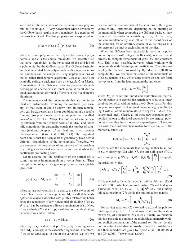
2.1. Noise-free geometric constraints

At the jth configuration of the calibration board, j =1, . . . , M , (see Figure 2), the fiducial markers whose posi-tions are known with respect to the calibration board’s frameof reference {Bj}, are first detected in the camera’s image.The 6 d.o.f. transformation between {C} and {Bj} is thencomputed using a PnP algorithm (Quan and Lan 1999;Ansar and Daniilidis 2003; Hesch and Roumeliotis 2011),

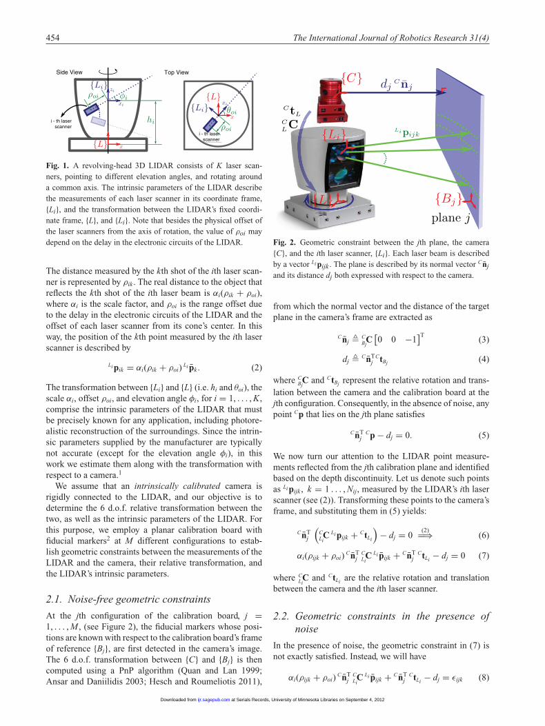
Fig. 2. Geometric constraint between the jth plane, the camera{C}, and the ith laser scanner, {Li}. Each laser beam is describedby a vector Li pijk . The plane is described by its normal vector Cnj

and its distance dj both expressed with respect to the camera.

from which the normal vector and the distance of the targetplane in the camera’s frame are extracted as

Cnj � CBjC

[0 0 −1

]T(3)

dj � CnTj

CtBj (4)

where CBjC and CtBj represent the relative rotation and trans-

lation between the camera and the calibration board at thejth configuration. Consequently, in the absence of noise, anypoint Cp that lies on the jth plane satisfies

CnTj

Cp − dj = 0. (5)

We now turn our attention to the LIDAR point measure-ments reflected from the jth calibration plane and identifiedbased on the depth discontinuity. Let us denote such pointsas Lipijk , k = 1 . . . , Nij, measured by the LIDAR’s ith laserscanner (see (2)). Transforming these points to the camera’sframe, and substituting them in (5) yields:

CnTj

(CLiC Li pijk + CtLi

)− dj = 0

(2)=⇒ (6)

αi(ρijk + ρoi)CnT

jCLiC Li pijk + CnT

jCtLi − dj = 0 (7)

where CLiC and CtLi are the relative rotation and translation

between the camera and the ith laser scanner.

2.2. Geometric constraints in the presence ofnoise

In the presence of noise, the geometric constraint in (7) isnot exactly satisfied. Instead, we will have

αi(ρijk + ρoi)CnT

jCLiC Li pijk + CnT

jCtLi − dj = εijk (8)



Mirzaei et al. 455

where εijk is the residual due to the noise in the image andthe LIDAR measurements. The covariance of this residualis

σ 2εijk

=(αi

CnTj

CLiC Li pijk

)2σ 2

ρ + hpijk RphTpijk

+ hnRnj hTn + σ 2

dj(9)

where σρ is the standard deviation of noise in ρijk , and σdj isthe standard deviation of the uncertainty in dj. The covari-ance of the uncertainty in the laser beam directions, Li pijk ,and the plane normal vector, Cnj, expressed in their localtangent planes (see Hartley and Zisserman 2004, Appendix6.9.3), are represented by Rp and Rnj , respectively. Thecorresponding Jacobians are

hpijk = αi(ρijk + ρoi)CnT

jCLiC Hpijk

[I2 02×1

]T(10)

hnj =(αi(ρijk + ρoi)

Li pTijk

CLiCT + CtT

Li

)Hnj

[I2 02×1

]T

(11)

where Hu is the 3 × 3 Householder matrix associated withthe unit vector u (Golub and van Loan 1996), defined as

Hu � I3 − 2vvT

vTv, v � u + sign( eT

3 u) e3, e3 � [0 0 1]T.

(12)

Note that the characteristics of εijk depend not only on theuncertainty of the measurements, but also on the unknowncalibration parameters.

2.3. Structural constraints

In addition to the camera and laser scanner measurements,the following constraints can also be used to increase theaccuracy of the calibration process. Specifically, since thez-axis of {Li} is aligned with the z-axis of {L}, while theirx-axes form an angle θoi, the following constraint holds forall C

LiC:

CLiC = C

LCCz( θoi) (13)

where Cz( θoi) represents a rotation around the z-axis by anangle θoi. In addition, the origin of each laser-scanner framelies on the z-axis of {L} with vertical offset of hi from theorigin of {L}, resulting in the following constraint:

CLC

T ( CtLi − CtL) = [0 0 hi]T. (14)

3. Algorithm description

In order to estimate the unknown calibration parameters,we form a constrained nonlinear least-squares cost func-tion from the residuals of the geometric constraint over allpoint and plane observations (see (8)). To minimize thisleast-squares cost, one has to employ iterative minimizerssuch as the Levenberg–Marquardt (Press et al. 1992), that

Algorithm 1 Estimate intrinsic LIDAR and extrinsicLIDAR–camera calibration parameters.

1: for jth configuration of the calibration plane do2: Record an image and a LIDAR snapshot.3: Detect the known fiducial markers on the image.4: Compute Cnj and dj using a PnP algorithm.5: for ith laser scanner do6: Identify the laser points hitting the calibration

plane using depth discontinuity.7: Compute the contributions of jth plane’s observa-

tion to the rotation-offset optimality equations (see(23)).

8: end for9: end for

10: for ith laser scanner do11: Solve the optimality equations in (23) to compute

critical points of (21).12: Estimate si and ρoi as the critical point that mini-

mizes (22).13: Solve the linear least-squares problem in (31) to

estimate CtLi and αi.14: end for15: Refine the estimates for all of the unknowns and

enforce (13) and (14) by iteratively minimizing (32).

require a precise initial estimate to ensure convergence. Toprovide accurate initialization, in this section we presenta novel analytical method to estimate the LIDAR–cameratransformation and all intrinsic parameters of the LIDAR(except the elevation angle φi which is precisely knownfrom the manufacturer). In order to reduce the complex-ity of the initialization process, we temporarily drop theconstraints in (13) and (14) and seek to determine thetransformation between the camera and each of the laserscanners (along with each scanner’s intrinsic parameters)independently (see Sections 3.1–3.3). Once an accurate ini-tial estimate is computed, we lastly perform an iterativenonlinear least-squares refinement that explicitly considers(13) and (14), and increases the calibration accuracy (seeSection 3.4).

3.1. Analytical estimation of offset and relativerotations

Note that the term CnTj

CtLi − dj in (7) is constant for allpoints k of the ith laser scanner that hit the calibration planeat its jth configuration. Therefore, subtracting two noise-free constraints of the form (7) for the points Lipijk and Lipijl,and dividing the result by the non-zero scale, αi, yields

CnTj

CLiC(ui

jkl + ρoivijkl) = 0 (15)

where uijkl � ρijk

Li pijk − ρijlLi pijl and vi

jkl � Li pijk − Li pijl.Note that this constraint involves as unknowns only the rel-ative rotation of the ith laser scanner with respect to thecamera, C

LiC, and its offset, ρoi. Let us express the former,




CLiC, using the Cayley–Gibbs–Rodriguez (CGR) parameteri-

zation (Shuster 1993), i.e.

CLiC(s) = C( si)

1 + sTi si

(16)

C( si) �((1 − sT

i si) I3 + 2�si ×� + 2sisTi

)(17)

where sTi = [si1 si2 si3] is the vector of CGR parameters

that represent the relative orientation of the ith laser scannerwith respect to the camera, and

�s ×� �

⎡⎣ 0 −s3 s2

s3 0 −s1

−s2 s1 0

⎤⎦ (18)

is the corresponding skew-symmetric matrix. Substituting(16) in (15), and multiplying both sides with the non-zeroterm 1 + sT

i si yields

CnTj C(si) (ui

jkl + ρoivijkl) = 0. (19)

This algebraic constraint holds exactly in the absence ofnoise. In that case, the method presented in Section 4can be employed to recover the unknowns given the min-imum number of measurements. In the presence of noise,however, (19) becomes

CnTj C(si) (ui

jkl + ρoivijkl) = ηi

jkl (20)

where ηijkl is a non-zero residual. In this case, we estimate

si and ρoi by solving the following nonlinear least-squaresproblem:

si, ρoi = minsi,ρoi

Ci (21)

Ci � 1

2

M∑j=1

Nij2∑

k=1

Nij∑l= Nij

2 +1

(CnT

j C( si) ( uijkl + ρoiv

ijkl)

)2(22)

where, without loss of generality, we have assumed that Nij

is even. Note that the Nij points from the ith laser scanner,and the jth configuration of the calibration plane are dividedinto two mutually exclusive groups so as to ensure that eachpoint appears in the least-squares cost only once and henceavoid noise correlations.

When a sufficient number of plane configurations areobserved, we employ a recently proposed algebraic methodto directly solve this nonlinear least-squares problem with-out requiring initialization (Trawny and Roumeliotis 2010).Specifically, we first form the following polynomial systemdescribing the optimality conditions of (21):

fi = ∂Ci

∂si= 0, = 0, . . . , 3, and si0 � ρoi. (23)

Note that the cost function in (22) is a polynomial of degreesix in the elements of si and ρoi. Therefore, (23) consistsof four polynomials of degree five in four variables. The

detailed derivation of these polynomials is provided inAppendix A. This polynomial system has 243 solutions thatcomprise the critical points of the least-squares cost func-tion Ci, and can be computed using the eigenvalue decom-position of the so-called multiplication matrix (see Section3.2). The globally optimal solution of the least-squaresproblem is the critical point that minimizes (22), and it isselected through direct evaluation of the cost function Ci.We point out that the computational complexity of solving(23) and finding the global minimum does not increase withthe addition of measurements, since the degree and numberof polynomials expressing the optimality conditions arefixed regardless of the number of calibration-plane con-figurations and laser-scanner points reflected from them.Moreover, computing the contribution of all points to thecoefficients of the polynomials fi, = 0, . . . , 3, increasesonly linearly with the number of measurements.

3.2. Polynomial system solver

Several methods exist for solving the polynomials describ-ing the optimality conditions of (23). Amongst them,numerical methods, such as Newton–Raphson, need properinitialization and may not find all of the solutions. Symbolicreduction methods based on the computation of the system’sGröbner basis are capable of finding all roots without anyinitialization (Cox et al. 2004). However, they can only beused for integer or rational coefficients since their applica-tion to floating-point numbers suffers from quick accumula-tion of round-off errors, which, in turn, results in incorrectsolutions (Cox et al. 2004). Instead, we employ a methoddeveloped by Auzinger and Stetter (1988) that computes ageneralization of the companion matrix to systems of mul-tivariate polynomial equations, namely the multiplicationmatrix, whose eigenvalues are the roots of the associatedpolynomial system. In the following, we briefly describe anefficient method for computing the multiplication matrix. InAppendix C, a simple example is provided to demonstratehow this method is applied in practice.

Let us denote a monomial in x = [x1 · · · xn]T by xγ �xγ1

1 xγ22 · · · xγn

n , γi ∈ Z≥0, with degree∑n

i=1 γi. A polyno-mial of degree d in x is denoted by f = cTxd where xd isthe

(n+d

n

)-dimensional vector of monomials of degree up to

and including d, and c is the vector of coefficients of equalsize. We assume that the given system of equations has npolynomials, denoted by fi = cT

i xdi = 0, i = 1, . . . , n,each of them with degree di. The total degree of the poly-nomial system is d � maxi di. By padding the coefficientvectors of fi with zeros, and stacking them together in C,we can present the polynomial system in the matrix form ofCxd = 0.

A system of polynomial equations defines an ideal I asthe set of all of the polynomials that can be generated as∑

i fihi where hi is any polynomial in x. Clearly the ele-ments of the ideal become zero at the solutions of theoriginal (generator) polynomial system. The Gröbner basisG � 〈g1, . . . gt〉 of an ideal is a finite subset of the ideal



Mirzaei et al. 457

such that (i) the remainder of the division of any polyno-mial to it is unique, (ii) any polynomial whose division bythe Gröbner basis results in zero remainder, is a member ofthe associated ideal. The first property can be expressed as

ϕ( x) = r( x) +t∑

i=1

gi( x) hi( x) (24)

where ϕ is any polynomial in x, hi are the quotient poly-nomials, and r is the unique remainder. We hereafter usethe name ‘remainder’ as the remainder of the division ofa polynomial by the Gröbner basis. The Gröbner basis foran ideal generated from polynomials with integer or ratio-nal numbers can be computed using implementations ofthe so-called Buchberger’s algorithm (Cox et al. 2004) onsymbolic software packages such as Macaulay2 or Maple.Computation of the Gröbner basis for polynomials withfloating-point coefficients is much more difficult due toquick accumulation of round-off errors in the Buchberger’salgorithm.

The remainders of the polynomials that are not in anideal are instrumental in finding the solutions (i.e. vari-ety) of that ideal. It can be shown that all such remain-ders can be expressed as a linear combination of a specific(unique) group of monomials that comprise the so-callednormal set (Cox et al. 2004). The normal set can be eas-ily obtained from the Gröbner basis of an ideal, and undermild conditions,3 its cardinality equals the number of solu-tions (real and complex) of the ideal, and it will containthe monomial 1 (Cox et al. 2004, p.43). The importantpoint here is that the normal set is generically fixed acrossdifferent instantiations of the polynomials. Therefore, wecan compute the normal set of an instance of the problem(e.g. integer or rational coefficients) and use it when thecoefficients are floating point.

Let us assume that the cardinality of the normal set iss, and represent its monomials in a vector form xB. Thenmultiplication of xB with a generic polynomial ϕ( x) yields(see (24)):

ϕ( x) · xB = MϕxB +

⎡⎢⎣

h11 · · · h1t...

...hs1 · · · hst

⎤⎥⎦

⎡⎢⎣

g1...

gt

⎤⎥⎦ (25)

where hij are polynomials in x and gi are the elements ofthe Gröbner basis. In this expression, Mϕ is called the mul-tiplication matrix associated with ϕ. This relationship holdssince the remainder of any polynomial (including xγ ϕ( x),xγ ∈ xB) can be written as a linear combination of xB. Now,if we evaluate (25) at x = p, a solution of the ideal, all gi

become zero, and we obtain

ϕ( p) · pB = MϕpB (26)

where pB is xB evaluated at p. Clearly, pB is an eigenvec-tor of Mϕ , and ϕ(p) is the associated eigenvalue. Therefore,if we select ϕ(x) equal to one of the variables (e.g. xi), we

can read off the xi-coordinate of the solutions as the eigen-values of Mϕ . Furthermore, depending on the ordering ofthe monomials when computing the Gröbner basis, xB mayinclude all first-order monomials x1, . . . , xn. In that case,one can simultaneously read off all of the coordinates ofthe solutions, for an arbitrary choice of ϕ, as long as it isnon-zero and distinct at each solution of the ideal.

When the Gröbner basis is available (such as in poly-nomial systems with integer coefficients), one can use itdirectly to compute remainders of ϕ(x) · xB, and constructMϕ . This is not possible, however, when working withpolynomials with floating-point coefficients. Therefore weemploy the method proposed by Byröd et al. (2008) tocompute Mϕ . We first note that some of the monomials ofϕ( x) ·xB remain in xB, while some others do not. We formthe vector xR from the latter monomials, and write

ϕ(x) · xB = M′ϕ

[xR

xB

](27)

where M′ϕ is called the unreduced multiplication matrix.

Our objective is to express the remainders of xR as a linearcombination of xB without using the Gröbner basis. For thispurpose, we expand each original polynomial fi by multiply-ing it with all of the monomials up to degree − di ( to bedetermined later). Clearly all of these new expanded poly-nomials belong to the ideal generated by the original poly-nomials, and they have monomials up to degree . Thus, wecan write them collectively in matrix form as Cex = 0. Wereorder x and Ce as

Cex = [CE CR CB

] ⎡⎣xE

xR

xB

⎤⎦ = 0 (28)

where xE are the monomials that belong neither to xR norto xB. Multiplying (28) with NT, the left null space of CE,

and decomposing NTCR = QR = [Q1 Q2]

[R1

0

]using QR

factorization, yields:

[NTCR NTCB

] [xR

xB

]= Q

[R1 QT

1 NTCB

0 QT2 NTCB

] [xR

xB

]= 0.

(29)

If is selected sufficiently large, R1 will be full rank (Reidand Zhi 2009), which allows us to solve (29) and find xR asa function of xB, i.e. xR = −R−1

1 QT1 NTCBxB. Substituting

this relationship in (27) yields the multiplication matrix:

Mϕ = M′ϕ

[Is

−R−11 QT

1 NTCB

]. (30)

For solving equations (23), we had to expand the polyno-mials up to degree = 15 and arrived at a multiplicationmatrix Mϕ of dimensions 243 × 243. Finally, we mentionthat it is possible to compute the multiplication matrix with-out explicit computation of the normal set. Further detailson this subject and also on possible numerical instabilitiesand their remedies are given by Byröd et al. (2008); Reidand Zhi (2009); Trawny et al. (2009).




3.3. Analytical estimation of scale and relativetranslation

Once the relative rotation, CLi

C, and offset, ρoi, of eachlaser scanner, i = 1, . . . , K, is computed, we use linearleast-squares to determine the relative translation and scalefrom (7). Specifically, we stack together all of the measure-ment constraints on the ith laser scanner’s scale and rela-tive translation (from different points and calibration-planeconfigurations), and write them in a matrix form as

⎡⎢⎢⎢⎣

CnT1 (ρi11 + ρoi) CnT

1CLiC Li pi11

CnT1 (ρi12 + ρoi) CnT

1CLiC Li pi12

......

CnTM (ρiMNiM + ρoi) CnT

MCLiC Li piMNiM

⎤⎥⎥⎥⎦

[CtLi

αi

]=

⎡⎢⎢⎢⎣

d1

d1...

dM

⎤⎥⎥⎥⎦ .

(31)

Under the condition that the coefficient matrix on the left-hand side of this equality is full rank (see Section 5), wecan easily obtain the ith laser scanner’s scale factor, αi, andrelative translation, CtLi , by solving (31).

3.4. Iterative refinement

Once the initial estimates for the transformation betweenthe camera and the laser scanners, and the intrinsic parame-ters of the LIDAR are known (Sections 3.1–3.3), we employan iterative refinement method to enforce the constraints in(13) and (14). Specifically, we choose the coordinate frameof one of the laser scanners (e.g. the first laser scanner) asthe LIDAR’s fixed coordinate frame, i.e. {L} = {L1}. Thenfor {Li}, i = 2, . . . , K, we employ the estimated relativetransformation with respect to the camera (i.e. C

LiC and CtLi )

to obtain the relative transformations between {Li} and {L}.From these relative transformations, we only use the z com-ponent of the translation to initialize each laser scanner’svertical offset, hi (see (14)), and the yaw component of therotation to initialize each laser scanner’s θoi (see (13)).

We then formulate the following constrained minimiza-tion problem to enforce (13) and (14):

min∑i,j,k

[αi(ρijk + ρoi) CnT

jCLiC Li pijk + CnT

jCtLi − dj

]2

σ 2εijk

subject to: CLiC = C

LCCz(θoi)

CLC

T (CtLi − CtL) = [0 0 hi]T (32)

where the optimization variables are αi, ρoi, θoi, hi, i =2, . . . , K, α1, ρo1, CtL, C

L C, and σ 2εijk

is defined in (9).4 Notethat the constraints in (32) should be taken into accountusing the method of Lagrange multipliers. Alternatively,we minimized a reformulation of (32) that uses a minimalparameterization of the unknowns to avoid the constraints(and, hence, the Lagrange multipliers). The details of thisalternative cost function are provided in Appendix D.

4. Identifiability conditions

In this section, we examine the conditions under which theunknown LIDAR–camera transformation and the intrinsicparameters of the LIDAR are identifiable, and thus can beestimated using the algorithms in Sections 3.1–3.4.

4.1. Observation of one plane

Suppose that we are provided with LIDAR measurementsthat lie only on one plane whose normal vector is denotedas Cn1. In this case, it is easy to show that the measurementconstraint in (6) does not change if C

LiC is perturbed by a

rotation around Cn1, represented by the rotation matrix C′:

CnT1 C′ C

LiC Li pi1k + CnT

1CtLi − d1 = 0 (33)

=⇒ CnT1

CLiC Li pi1k + CnT

1CtLi − d1 = 0. (34)

The second equation is obtained from the first, since Cn1 isan eigenvector of C′, thus CnT

1 C′ = CnT1 . Therefore, when

observing only one plane, any rotation around the plane’snormal vector is unidentifiable. Similarly, if we perturb CtLi

by a translation parallel to the plane, represented by t′, themeasurement constraint does not change:

CnT1

CLiC Li pi1k + CnT

1 ( CtLi + t′) −d1 = 0 (35)

=⇒ CnT1

CLiC Li pi1k + CnT

1CtLi − d1 = 0. (36)

This relationship holds since CnT1 t′ = 0. Therefore, when

observing only one plane, any translation parallel to theplane’s normal is unidentifiable.

4.2. Observation of two planes

Consider now that we are provided with measurements fromtwo planes, described by Cn1, d1, Cn2, d2. If we perturbthe laser scanner’s relative translation with t′′ ∝ Cn1 ×Cn2 (see (35)), none of the measurement constraints willchange, since CnT

1 t′′ = CnT2 t′′ = 0. Therefore, we conclude

that the relative translation cannot be determined if only twoplanes are observed.

4.3. Observation of three planes

In this section, we prove that when three planes with linearlyindependent normal vectors are observed, we can determineall of the unknowns. For this purpose, we first determine therelative orientation C

LiC and the offset ρoi and then find the

scale αi and relative translation CtLi . Let us assume that theith laser scanner has measured four points on each plane,denoted as (ρijk , Li pijk) , j = 1, 2, 3, k = 1, . . . , 4. Eachof these points provides one constraint of the form (7). Wefirst eliminate the unknown relative translation and scale,by subtracting the constraints for point k = 1 from k = 2,



Mirzaei et al. 459

point k = 2 from k = 3, and point k = 3 from k = 4, andobtain

CnTj

CLiC

(ui

j12 + ρoi vij12

)= 0 (37)

CnTj

CLiC

(ui

j23 + ρoi vij23

)= 0 (38)

CnTj

CLiC

(ui

j34 + ρoi vij34

)= 0 (39)

where uijkl � ρijk

Li pijk − ρijlLi pijl, vi

jkl � Li pijk − Li pijl, andj = 1, 2, 3. Note that Li pijk and Li pijl lie on the intersectionof the unit sphere and the cone specified by the beams ofthe ith laser scanner. Since the intersection of a co-centricunit sphere and a cone is always a circle, we conclude thatall vi

jkl for a given i belong to a plane and have only 2 d.o.f.

Thus, we can write vij34 as a linear combination of vi

j12 and

vij23, i.e.

vij34 = a vi

j12 + b vij23 (40)

for some known scalars a and b. Substituting this relation-ship in (39), and using (37)-(38) to eliminate the termscontaining ρoi yields

CnTj

CLiC

(ui

j34 − a uij12 − b ui

j23

)= 0 (41)

for j = 1, 2, 3. The only unknown in this equation is therelative orientation C

LiC of the ith laser scanner. These equa-

tions are identical to those for orientation estimation usingline-to-plane correspondences, which is known to have atmost eight solutions that can be analytically computed whenCnj, j = 1, 2, 3, are linearly independent (Chen 1991). OnceCLiC is known, we can use any of (37)–(39) to compute the

offset ρoi. Finally, the scale and the relative translation canbe obtained from (31).

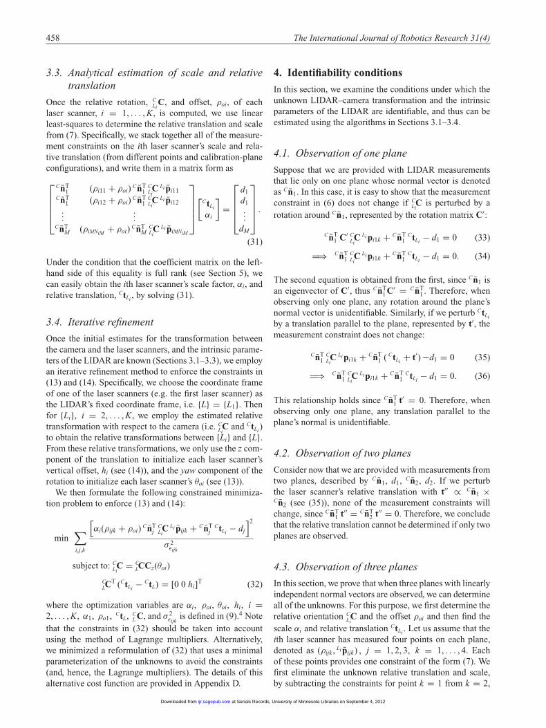
5. Experiments

5.1. Setup

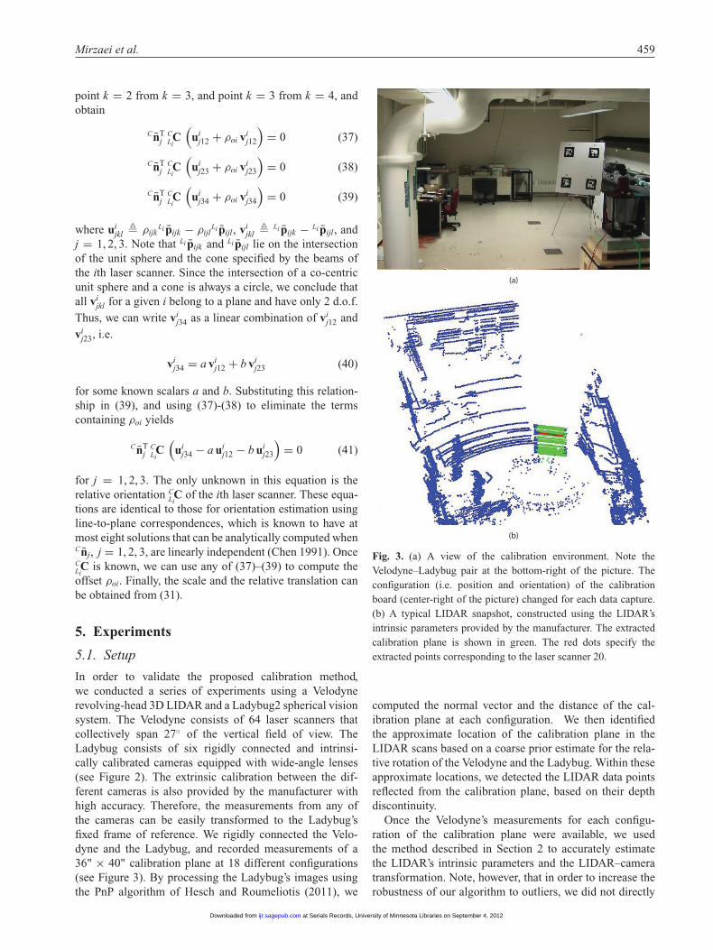
In order to validate the proposed calibration method,we conducted a series of experiments using a Velodynerevolving-head 3D LIDAR and a Ladybug2 spherical visionsystem. The Velodyne consists of 64 laser scanners thatcollectively span 27◦ of the vertical field of view. TheLadybug consists of six rigidly connected and intrinsi-cally calibrated cameras equipped with wide-angle lenses(see Figure 2). The extrinsic calibration between the dif-ferent cameras is also provided by the manufacturer withhigh accuracy. Therefore, the measurements from any ofthe cameras can be easily transformed to the Ladybug’sfixed frame of reference. We rigidly connected the Velo-dyne and the Ladybug, and recorded measurements of a36" × 40" calibration plane at 18 different configurations(see Figure 3). By processing the Ladybug’s images usingthe PnP algorithm of Hesch and Roumeliotis (2011), we

(a)

(b)

Fig. 3. (a) A view of the calibration environment. Note theVelodyne–Ladybug pair at the bottom-right of the picture. Theconfiguration (i.e. position and orientation) of the calibrationboard (center-right of the picture) changed for each data capture.(b) A typical LIDAR snapshot, constructed using the LIDAR’sintrinsic parameters provided by the manufacturer. The extractedcalibration plane is shown in green. The red dots specify theextracted points corresponding to the laser scanner 20.

computed the normal vector and the distance of the cal-ibration plane at each configuration. We then identifiedthe approximate location of the calibration plane in theLIDAR scans based on a coarse prior estimate for the rela-tive rotation of the Velodyne and the Ladybug. Within theseapproximate locations, we detected the LIDAR data pointsreflected from the calibration plane, based on their depthdiscontinuity.

Once the Velodyne’s measurements for each configu-ration of the calibration plane were available, we usedthe method described in Section 2 to accurately estimatethe LIDAR’s intrinsic parameters and the LIDAR–cameratransformation. Note, however, that in order to increase therobustness of our algorithm to outliers, we did not directly




use the raw laser points measured by the LIDAR. Instead,for each laser scanner, we fit small line segments to theintersection of the laser scanner’s beam and the calibrationplane, and used the endpoints of these line segments as theLIDAR’s measurements.5

5.2. Implemented methods

We compared the accuracy and consistency of the cali-bration parameters estimated by our proposed algorithm(denoted as AlgBLS), with the results of the approach pre-sented by Pandey et al. (2010) (denoted as PMSE), andwith those when using the calibration parameters providedby the manufacturer (intrinsic parameters only, denoted asFactory). Note that the PMSE only calibrates the offsetin the range measurements of each laser scanner (i.e. ρoi;see (2)), while for the rest of the parameters it uses theFactory values.

We implemented the PMSE as follows: for eachcalibration-plane configuration, we transformed the laserpoints reflected from the plane surface to the LIDAR’sEuclidean frame (see (1), (2), (13), and (14)) based onthe Factory parameters, and fitted a plane to them usingRANSAC (Hartley and Zisserman 2004). In the next step,we employed least-squares to minimize the distance ofthe laser points from the fitted planes by optimizing overthe range offsets, ρoi. The Euclidean coordinates of thelaser points are then adjusted accordingly, and processedto fit new planes using RANSAC; these re-fitted planesare used, in turn, to re-estimate the range offsets. Thisprocess is continued until convergence, or until a maximumnumber of iterations is reached. Once the range offsetswere calibrated, we minimized a least-square cost functionsimilar to (32), but only over the extrinsic calibrationparameters (i.e. C

L C and CtL).

5.3. Consistency of intrinsic parameters

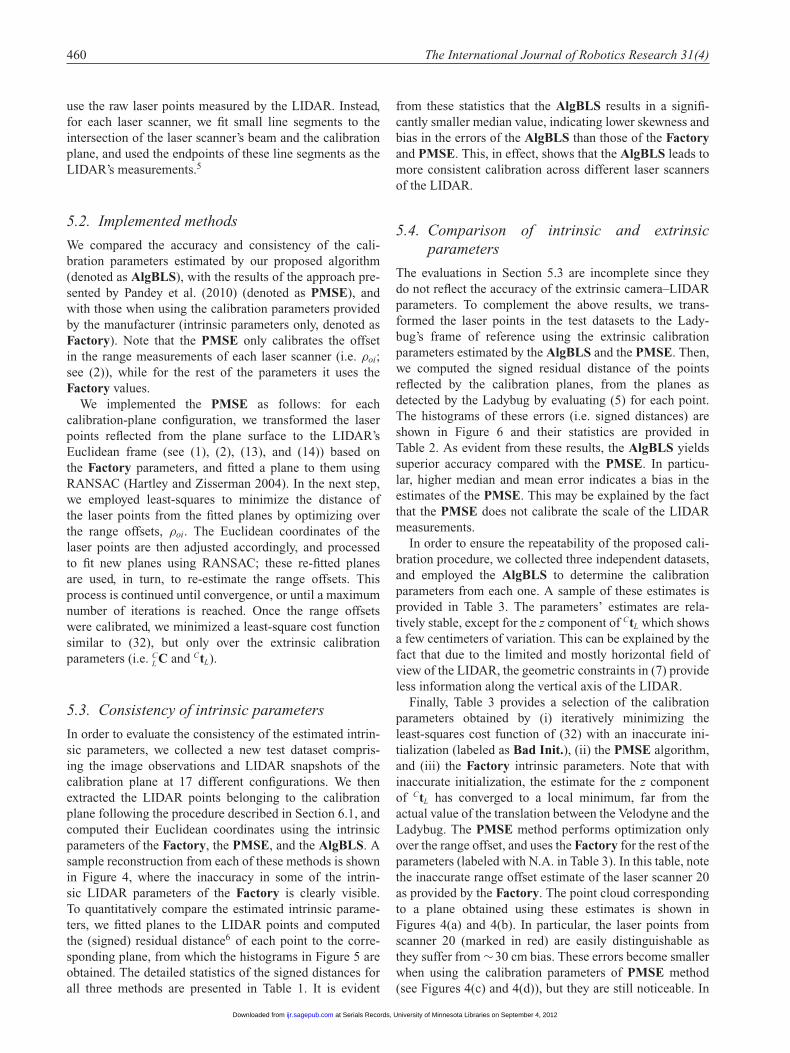
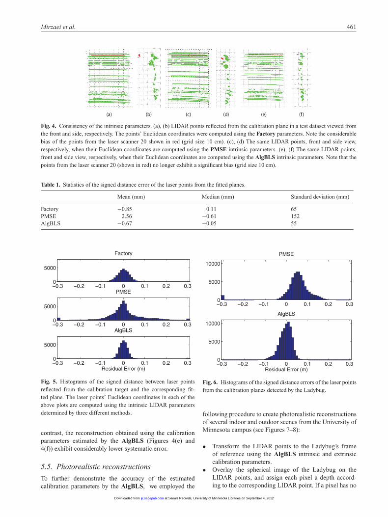
In order to evaluate the consistency of the estimated intrin-sic parameters, we collected a new test dataset compris-ing the image observations and LIDAR snapshots of thecalibration plane at 17 different configurations. We thenextracted the LIDAR points belonging to the calibrationplane following the procedure described in Section 6.1, andcomputed their Euclidean coordinates using the intrinsicparameters of the Factory, the PMSE, and the AlgBLS. Asample reconstruction from each of these methods is shownin Figure 4, where the inaccuracy in some of the intrin-sic LIDAR parameters of the Factory is clearly visible.To quantitatively compare the estimated intrinsic parame-ters, we fitted planes to the LIDAR points and computedthe (signed) residual distance6 of each point to the corre-sponding plane, from which the histograms in Figure 5 areobtained. The detailed statistics of the signed distances forall three methods are presented in Table 1. It is evident

from these statistics that the AlgBLS results in a signifi-cantly smaller median value, indicating lower skewness andbias in the errors of the AlgBLS than those of the Factoryand PMSE. This, in effect, shows that the AlgBLS leads tomore consistent calibration across different laser scannersof the LIDAR.

5.4. Comparison of intrinsic and extrinsicparameters

The evaluations in Section 5.3 are incomplete since theydo not reflect the accuracy of the extrinsic camera–LIDARparameters. To complement the above results, we trans-formed the laser points in the test datasets to the Lady-bug’s frame of reference using the extrinsic calibrationparameters estimated by the AlgBLS and the PMSE. Then,we computed the signed residual distance of the pointsreflected by the calibration planes, from the planes asdetected by the Ladybug by evaluating (5) for each point.The histograms of these errors (i.e. signed distances) areshown in Figure 6 and their statistics are provided inTable 2. As evident from these results, the AlgBLS yieldssuperior accuracy compared with the PMSE. In particu-lar, higher median and mean error indicates a bias in theestimates of the PMSE. This may be explained by the factthat the PMSE does not calibrate the scale of the LIDARmeasurements.

In order to ensure the repeatability of the proposed cali-bration procedure, we collected three independent datasets,and employed the AlgBLS to determine the calibrationparameters from each one. A sample of these estimates isprovided in Table 3. The parameters’ estimates are rela-tively stable, except for the z component of CtL which showsa few centimeters of variation. This can be explained by thefact that due to the limited and mostly horizontal field ofview of the LIDAR, the geometric constraints in (7) provideless information along the vertical axis of the LIDAR.

Finally, Table 3 provides a selection of the calibrationparameters obtained by (i) iteratively minimizing theleast-squares cost function of (32) with an inaccurate ini-tialization (labeled as Bad Init.), (ii) the PMSE algorithm,and (iii) the Factory intrinsic parameters. Note that withinaccurate initialization, the estimate for the z componentof CtL has converged to a local minimum, far from theactual value of the translation between the Velodyne and theLadybug. The PMSE method performs optimization onlyover the range offset, and uses the Factory for the rest of theparameters (labeled with N.A. in Table 3). In this table, notethe inaccurate range offset estimate of the laser scanner 20as provided by the Factory. The point cloud correspondingto a plane obtained using these estimates is shown inFigures 4(a) and 4(b). In particular, the laser points fromscanner 20 (marked in red) are easily distinguishable asthey suffer from ∼30 cm bias. These errors become smallerwhen using the calibration parameters of PMSE method(see Figures 4(c) and 4(d)), but they are still noticeable. In



Mirzaei et al. 461

(a) (b) (c) (d) (e) (f)

Fig. 4. Consistency of the intrinsic parameters. (a), (b) LIDAR points reflected from the calibration plane in a test dataset viewed fromthe front and side, respectively. The points’ Euclidean coordinates were computed using the Factory parameters. Note the considerablebias of the points from the laser scanner 20 shown in red (grid size 10 cm). (c), (d) The same LIDAR points, front and side view,respectively, when their Euclidean coordinates are computed using the PMSE intrinsic parameters. (e), (f) The same LIDAR points,front and side view, respectively, when their Euclidean coordinates are computed using the AlgBLS intrinsic parameters. Note that thepoints from the laser scanner 20 (shown in red) no longer exhibit a significant bias (grid size 10 cm).

Table 1. Statistics of the signed distance error of the laser points from the fitted planes.

Mean (mm) Median (mm) Standard deviation (mm)

Factory −0.85 0.11 65PMSE 2.56 −0.61 152AlgBLS −0.67 −0.05 55

−0.3 −0.2 −0.1 0 0.1 0.2 0.30

5000

Factory

−0.3 −0.2 −0.1 0 0.1 0.2 0.30

5000

PMSE

−0.3 −0.2 −0.1 0 0.1 0.2 0.30

5000

AlgBLS

Residual Error (m)

Fig. 5. Histograms of the signed distance between laser pointsreflected from the calibration target and the corresponding fit-ted plane. The laser points’ Euclidean coordinates in each of theabove plots are computed using the intrinsic LIDAR parametersdetermined by three different methods.

contrast, the reconstruction obtained using the calibrationparameters estimated by the AlgBLS (Figures 4(e) and4(f)) exhibit considerably lower systematic error.

5.5. Photorealistic reconstructions

To further demonstrate the accuracy of the estimatedcalibration parameters by the AlgBLS, we employed the

−0.3 −0.2 −0.1 0 0.1 0.2 0.30

5000

10000

PMSE

−0.3 −0.2 −0.1 0 0.1 0.2 0.30

5000

10000

AlgBLS

Residual Error (m)

Fig. 6. Histograms of the signed distance errors of the laser pointsfrom the calibration planes detected by the Ladybug.

following procedure to create photorealistic reconstructionsof several indoor and outdoor scenes from the University ofMinnesota campus (see Figures 7–8):

• Transform the LIDAR points to the Ladybug’s frameof reference using the AlgBLS intrinsic and extrinsiccalibration parameters.

• Overlay the spherical image of the Ladybug on theLIDAR points, and assign each pixel a depth accord-ing to the corresponding LIDAR point. If a pixel has no




Table 2. Statistics of the signed distance error of the laser points from the calibration planes detected by the Ladybug.

Mean (mm) Median (mm) Standard deviation (mm)

PMSE 40 55 151AlgBLS −4.3 −1.4 28

Table 3. A sample of the estimated calibration parameters. The first three rows show a selection of calibration parameters as estimatedby AlgBLS for three different datasets. The column labeled as rpy represents roll, pitch, and yaw of C

L C. Rows 4–6 show a selectionof calibration parameters that are obtained by other methods. Note that the scale parameters αi are unitless, and N.A. indicates non-applicable fields.

Number rpy (deg) CtL (cm) α1 ρo1 (cm) α20 ρo20 (cm) θo20 (deg) h20 (cm)of planes

AlgBLS 1 18[1.31 1.27 −88.45

][−2.5 0.04 −20.10] 1.02 99.49 1.01 100.88 36.91 −3.71

AlgBLS 2 17[1.62 0.79 −88.40

][−1.64 0.19 −12.92] 1.01 101.83 1.00 101.82 36.03 −4.98

AlgBLS 3 18 [1.26 0.84 −88.43] [−2.07 −0.12 −17.95] 1.01 101.05 0.98 105.94 36.05 −0.85Bad Init. 18 [0.34 −0.63 −87.93] [−1.64 −0.50 −117.08] 1.01 98.99 0.99 104.49 34.95 98.31PMSE 18 [3.19 −0.97 −88.32] [1.40 −2.12 −53.64] N.A. 91.49 N.A. 90.85 N.A. N.A.Factory 18 N.A. N.A. 1 95.50 1 66.53 34.95 −0.24

corresponding LIDAR point, compute an approximatedepth by linearly interpolating the nearest laser points.

• Render 3D surfaces from the 3D pixels using Delaunaytriangulation (de Berg et al. 2008).

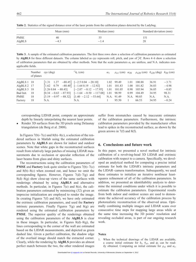
In Figures 7(b)–7(c) and 8(b)–8(c), a selection of the ren-dered surfaces in Matlab using the estimated calibrationparameters by AlgBLS are shown for indoor and outdoorscenes. Note that white gaps in the reconstructed surfacesresult from relatively large patches of missing LIDAR mea-surements due to occlusion or specular reflection of thelaser beams from glass and shiny surfaces.

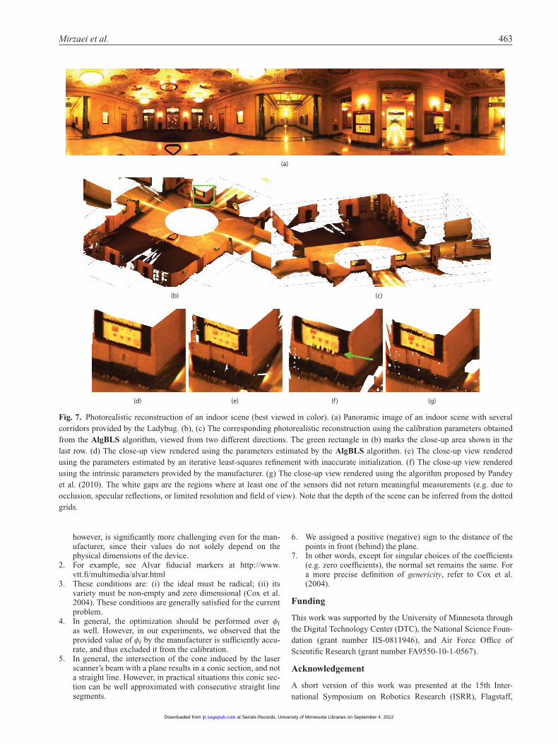
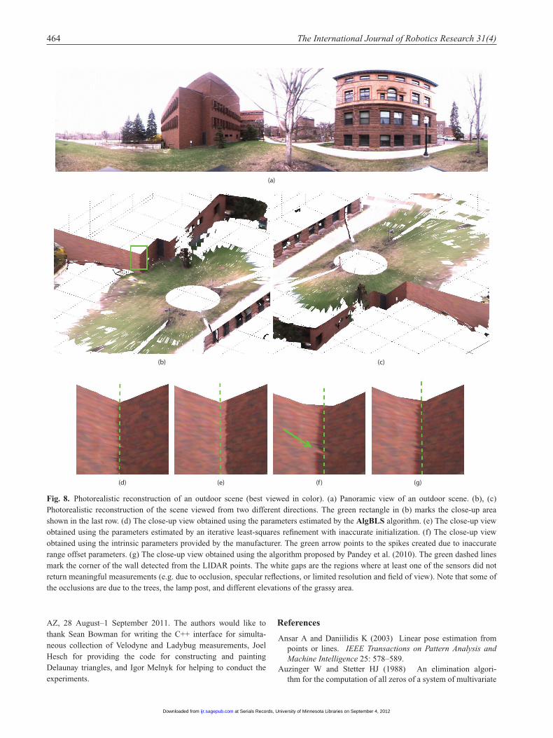
The reconstructions using the calibration parameters ofPMSE and Factory look quite similar to Figures 7(b)–7(c)and 8(b)–8(c) when zoomed out, and hence we omit thecorresponding figures. However, Figures 7(d)–7(g) and8(d)–8(g) show close-up views of the same surfaces withrenderings obtained by using AlgBLS and alternativemethods. In particular, in Figures 7(e) and 8(e), the cali-bration parameters estimated by minimizing (32) given animprecise initialization are employed to render the image.In creating Figures 7(f) and 8(f), we have only estimatedthe extrinsic calibration parameters, and used the Factoryintrinsic parameters. Finally Figures 7(g) and 8(g) arerendered using the estimated calibration parameters byPMSE. The superior quality of the renderings obtainedusing the calibration parameters of the AlgBLS is clearin these images. In particular, in Figures 8(d)–8(g), thelines corresponding to the corner of the wall are estimatedbased on the LIDAR measurements, and depicted as greendashed line. Given a perfect calibration, the shadow edgeof the overlaid image should match the extracted corner.Clearly, while the rendering by AlgBLS provides an almostperfect match between the two, the other rendered images

suffer from mismatches caused by inaccurate estimatesof the calibration parameters. Furthermore, the intrinsiccalibration parameters provided by the manufacturer oftenlead to spikes in the reconstructed surface, as shown by thegreen arrows in 7(f) and 8(f).

6. Conclusions and future work

In this paper, we presented a novel method for intrinsiccalibration of a revolving-head 3D LIDAR and extrinsiccalibration with respect to a camera. Specifically, we devel-oped an analytical method for computing a precise initialestimate for both the LIDAR’s intrinsic parameters andthe LIDAR–camera transformation. Subsequently, we usedthese estimates to initialize an iterative nonlinear least-squares refinement of all of the calibration parameters. Inaddition, we presented an identifiability analysis to deter-mine the minimal conditions under which it is possible toestimate the calibration parameters. Experimental resultsfrom both indoor and outdoor scenes are used to demon-strate the achieved accuracy of the calibration process byphotorealistic reconstruction of the observed areas. Opti-mally combining multiple images and LIDAR scans overconsecutive time steps for mapping large areas while atthe same time increasing the 3D points’ resolution andrevealing occluded areas, is part of our ongoing researchwork.

Notes

1. When the technical drawings of the LIDAR are available,a coarse initial estimate for hi, θoi, and φi can be read-ily obtained. Computing an initial estimate for ρoi and αi,



Mirzaei et al. 463

(a)

(b) (c)

(d) (e) (f) (g)

Fig. 7. Photorealistic reconstruction of an indoor scene (best viewed in color). (a) Panoramic image of an indoor scene with severalcorridors provided by the Ladybug. (b), (c) The corresponding photorealistic reconstruction using the calibration parameters obtainedfrom the AlgBLS algorithm, viewed from two different directions. The green rectangle in (b) marks the close-up area shown in thelast row. (d) The close-up view rendered using the parameters estimated by the AlgBLS algorithm. (e) The close-up view renderedusing the parameters estimated by an iterative least-squares refinement with inaccurate initialization. (f) The close-up view renderedusing the intrinsic parameters provided by the manufacturer. (g) The close-up view rendered using the algorithm proposed by Pandeyet al. (2010). The white gaps are the regions where at least one of the sensors did not return meaningful measurements (e.g. due toocclusion, specular reflections, or limited resolution and field of view). Note that the depth of the scene can be inferred from the dottedgrids.

however, is significantly more challenging even for the man-ufacturer, since their values do not solely depend on thephysical dimensions of the device.

2. For example, see Alvar fiducial markers at http://www.vtt.fi/multimedia/alvar.html

3. These conditions are: (i) the ideal must be radical; (ii) itsvariety must be non-empty and zero dimensional (Cox et al.2004). These conditions are generally satisfied for the currentproblem.

4. In general, the optimization should be performed over φias well. However, in our experiments, we observed that theprovided value of φi by the manufacturer is sufficiently accu-rate, and thus excluded it from the calibration.

5. In general, the intersection of the cone induced by the laserscanner’s beam with a plane results in a conic section, and nota straight line. However, in practical situations this conic sec-tion can be well approximated with consecutive straight linesegments.

6. We assigned a positive (negative) sign to the distance of thepoints in front (behind) the plane.

7. In other words, except for singular choices of the coefficients(e.g. zero coefficients), the normal set remains the same. Fora more precise definition of genericity, refer to Cox et al.(2004).

Funding

This work was supported by the University of Minnesota throughthe Digital Technology Center (DTC), the National Science Foun-dation (grant number IIS-0811946), and Air Force Office ofScientific Research (grant number FA9550-10-1-0567).

Acknowledgement

A short version of this work was presented at the 15th Inter-national Symposium on Robotics Research (ISRR), Flagstaff,




(a)

(b) (c)

(d) (e) (f) (g)

Fig. 8. Photorealistic reconstruction of an outdoor scene (best viewed in color). (a) Panoramic view of an outdoor scene. (b), (c)Photorealistic reconstruction of the scene viewed from two different directions. The green rectangle in (b) marks the close-up areashown in the last row. (d) The close-up view obtained using the parameters estimated by the AlgBLS algorithm. (e) The close-up viewobtained using the parameters estimated by an iterative least-squares refinement with inaccurate initialization. (f) The close-up viewobtained using the intrinsic parameters provided by the manufacturer. The green arrow points to the spikes created due to inaccuraterange offset parameters. (g) The close-up view obtained using the algorithm proposed by Pandey et al. (2010). The green dashed linesmark the corner of the wall detected from the LIDAR points. The white gaps are the regions where at least one of the sensors did notreturn meaningful measurements (e.g. due to occlusion, specular reflections, or limited resolution and field of view). Note that some ofthe occlusions are due to the trees, the lamp post, and different elevations of the grassy area.

AZ, 28 August–1 September 2011. The authors would like tothank Sean Bowman for writing the C++ interface for simulta-neous collection of Velodyne and Ladybug measurements, JoelHesch for providing the code for constructing and paintingDelaunay triangles, and Igor Melnyk for helping to conduct theexperiments.

References

Ansar A and Daniilidis K (2003) Linear pose estimation frompoints or lines. IEEE Transactions on Pattern Analysis andMachine Intelligence 25: 578–589.

Auzinger W and Stetter HJ (1988) An elimination algori-thm for the computation of all zeros of a system of multivariate



Mirzaei et al. 465

polynomial equations. In Proceedings of the InternationalConference on Numerical Mathematics, Singapore, pp. 11–30.

Byröd M, Josephson K and Åström K (2008) A column-pivotingbased strategy for monomial ordering in numerical Gröbnerbasis calculations. In Proceedings of the European Conferenceon Computer Vision, Marseille, France, pp. 130–143.

Chen HH (1991) Pose determination from line-to-plane cor-respondences: existence condition and closed-form solutions.IEEE Transactions on Pattern Analysis and Machine Intelli-gence 13: 530–541.

Cox D, Little J and O’Shea D (2004) Using Algebraic Geometry.Berlin: Springer.

de Berg M, Cheong O, van Kreveld M and Overmars M(2008) Computational Geometry: Algorithms and Applica-tions. Berlin: Springer-Verlag.

Fischler MA and Bolles RC (1981) Random sample consensus: Aparadigm for model fitting with applications to image analysisand automated cartography. Communications of the ACM 24:381–395.

Golub GH and van Loan CF (1996) Matrix Computations.Baltimore, MD: Johns Hopkins University Press.

Hartley RI and Zisserman A (2004) Multiple View Geometry inComputer Vision, 2nd edn. Cambridge: Cambridge UniversityPress.

Hesch JA and Roumeliotis SI (2011) A direct least-squares(DLS) solution for PnP. In Proceedings of the InternationalConference on Computer Vision, Barcelona, Spain.

Naroditsky O, Patterson A, IV, and Daniilidis K (2011) Auto-matic alignment of a camera with a line scan lidar system. InProceedings IEEE International Conference on Robotics andAutomation, Shanghai, China.

Pandey G, McBride J, Savarese S and Eustice R (2010) Extrin-sic calibration of a 3D laser scanner and an omnidirectionalcamera. In Proceedings IFAC Symposium on IntelligentAutonomous Vehicles, Lecce, Italy.

Press WH, Teukolsky SA, Vetterling WT and Flannery BP (1992)Numerical Recipes in C. Cambridge: Cambridge UniversityPress.

Quan L and Lan Z-D (1999) Linear n-point camera pose deter-mination. IEEE Transactions on Pattern Analysis and MachineIntelligence 21: 774–780.

Reid G and Zhi L (2009) Solving polynomial systems viasymbolic–numeric reduction to geometric involutive form.Journal of Symbolic Computation 44: 280–291.

Scaramuzza D, Harati A and Siegwart R (2007) Extrinsic selfcalibration of a camera and a 3D laser range finder from nat-ural scenes. In Proceedings IEEE/RSJ International Confer-ence on Intelligent Robots and Systems, San Diego, CA, pp.4164–4169.

Shuster MD (1993) A survey of attitude representations. Journalof Astronautical Science 41: 439–517.

Stamos I, Liu L, Chen C, Wolberg G, Yu G and Zokai S (2008)Integrating automated range registration with multiview geom-etry for the photorealistic modeling of large-scale scenes.International Journal of Computer Vision 78: 237–260.

Trawny N and Roumeliotis SI (2010) On the global optimum ofplanar, range-based robot-to-robot relative pose estimation. InProceedings IEEE International Conference on Robotics andAutomation, Anchorage, AK, pp. 3200–3206.

Trawny N, Zhou XS and Roumeliotis SI (2009) 3D relative poseestimation from six distances. In Proceedings of RoboticsScience and Systems, Seattle, WA.

Unnikrishnan R and Hebert M (2005) Fast Extrinsic Calibrationof a Laser Rangefinder to a Camera. Technical report, CarnegieMellon University, Robotics Institute.

Zhang Q and Pless R (2004) Extrinsic calibration of a cameraand laser range finder (improves camera calibration). InProceedings IEEE/RSJ International Conference IntelligentRobots and Systems, Sendai, Japan, pp. 2301–2306.

Appendix A

Notation

{Bj} coordinate frame of reference corresponding to thecalibration board at the jth configuration

{C} camera’s coordinate frame of reference

XY C rotation matrix representing the relative orientation of

{Y } w.r.t. {X }

dj distance of the calibration plane, at its jth configurationfrom the origin of {C}

hi vertical offset of the ith laser scanner w.r.t. {L}

In n × n identity matrix

{L} LIDAR’s coordinate frame of reference

{Li} coordinate frame of reference corresponding to the ithlaser scanner, i = 1, . . . , K

Cnj normal vector of the calibration plane, at its jth config-uration, w.r.t. {C}

Li pijk kth intrinsically corrected point, belonging to the cal-ibration board at its jth configuration, measured by theith laser scanner, w.r.t. {Li}

X tY relative position of {Y } w.r.t. {X }

w.r.t. with respect to

0m×n m × n matrix of zeros

αi scale factor of the ith laser scanner

φi elevation angle of the ith laser scanner

θoi azimuth angle between coordinate frames {L} and {Li}

θik azimuth angle of the kth shot of the ith laser scannerw.r.t. {Li}

ρik range measurement of the kth shot of the ith laserscanner w.r.t. {Li}

ρoi range offset of the ith laser scanner at Serials Records, University of Minnesota Libraries on September 4, 2012ijr.sagepub.comDownloaded from



Appendix B

The optimality conditions of (22) are as follows:

fi = ∂Ci

∂si=

M∑j=1

Nij2∑

k=1

Nij∑l= Nij

2 +1

(CnT


ijkl)

)

· ∂

∂si

(CnT


ijkl)

)︸︷︷︸

Ji

= 0. (42)

For = 1, 2, 3, Ji is

Ji = CnTj D( si) ( ui

jkl + ρoivijkl) (43)

where

D( si) = −2siI3 + 2�e ×� + 2esTi + 2sie

T (44)

e1 � [1 0 0]T, e2 � [0 1 0]T, e3 � [0 0 1]T (45)

and for = 0, i.e. si0 � ρoi, Ji0 = CnTj C( si) vi

jkl.

Appendix C

Consider the following simple example polynomials in x =[x1 x2]T:

f1 = x1 + x1x2 + 5 (46)

f2 = x21 + x2

2 − 10. (47)

These equations are of degree d1 = d2 = 2. The Gröbnerbasis of this polynomial system (using graded reverse lexordering (Cox et al. 2004)) is

g1 = x1x2 + x1 + 5 (48)

g2 = x21 + x2

2 − 10 (49)

g3 = x32 + x2

2 − 5x1 − 10x2 − 10 (50)

and, consequently, its normal set is

{1, x2, x1, x22}. (51)

Note that this normal set is generically7 the same for differ-ent coefficients of the system in (46)–(47). For example thefollowing system yields the same normal set:

f ′1 = 1.5x1 + e−1x2x1 + 0.5 (52)

f ′2 = 2.3x2

1 + 4

3x2

2 − π . (53)

Let us arrange the normal set in the vector form xB =[1, x2, x1, x2

2]T and choose ϕ( x) = x2. Then multiplying

ϕ( x) with xB and expressing the result in terms of xB andxR (see (27)) yields:

ϕ( x) xB =

⎡⎢⎢⎣

0 1 0 00 0 0 10 0 0 00 0 0 0

⎤⎥⎥⎦

⎡⎢⎢⎣

1x2

x1

x22

⎤⎥⎥⎦

︸︷︷︸xB

+

⎡⎢⎢⎣

0 00 01 00 1

⎤⎥⎥⎦

[x1x2

x32

]︸︷︷︸

xR

.

(54)

In order to express xR in terms of xB, we expand thepolynomials f1 and f2 up to degree = 3 by multiply-ing each of them with {1, x2, x1}. As a result, we obtainCe = [CE CR CB] where

CE =

⎡⎢⎢⎢⎢⎢⎢⎣

0 0 0 01 0 0 00 1 1 00 0 1 00 1 0 01 0 0 1

⎤⎥⎥⎥⎥⎥⎥⎦

, CR =

⎡⎢⎢⎢⎢⎢⎢⎣

1 01 00 00 00 10 0

⎤⎥⎥⎥⎥⎥⎥⎦

CB =

⎡⎢⎢⎢⎢⎢⎢⎣

5 0 1 00 5 0 00 0 5 0

−10 0 0 10 −10 0 00 0 −10 0

⎤⎥⎥⎥⎥⎥⎥⎦

.

Note that CE corresponds to xE = [x1x22 x2

1x2 x21 x3

1]T, i.e.the monomials that appear neither in xB nor in xR. Follow-ing the algebraic manipulations of (27)–(29), we obtain thefollowing multiplication matrix:

Mx2 =

⎡⎢⎢⎣

0 0 −5 101 0 0 100 0 −1 50 1 0 −1

⎤⎥⎥⎦ . (55)

In the next step, we compute the left eigenvectors of Mx2 ,and then scale them such that their first elements become 1(corresponding to the first element in xB). Consequently, thesolutions of the polynomial system are the elements of theeigenvectors that correspond to x1 and x2 in xB. Specifically,the set of solutions (i.e. variety) of (46)–(47) is[

x1

x2

]∈

{[−1.28562.8891

],

[−3.10260.6116

],

[2.1941 + 1.2056i

−2.7504 + 0.9618i

],

[2.1941 − 1.2056i

−2.7504 − 0.9618i

]}.

(56)

Appendix D

One approach for enforcing the constraints in (32) is to usethe method of Lagrange multipliers. It is possible, however,to re-parameterize the cost function and minimally expressit over the optimization variables. In this way, the con-straints in (32) will be automatically satisfied. Specifically,



Mirzaei et al. 467

we consider the kth intrinsically corrected point measuredby the ith laser scanner from the jth configuration of thecalibration plane as:

Lpijk =⎡⎣αi(ρijk + ρoi) cos φi cos(θijk + θoi)

αi(ρijk + ρoi) cos φi sin(θjik + θoi)αi(ρijk + ρoi) sin φi + hi

⎤⎦ . (57)

This relationship is obtained by substituting (1) in (2),and then transforming the result to the LIDAR’s frameof reference {L}. Note that the intrinsic LIDAR para-meters are already expressed in their minimal form; thusthe constraints in (32) are redundant and can be removed.In particular, (14) is satisfied since hi is added to the z

component of the point’s measurement and (13) is satisfiedsince θoi is added to the azimuth of the point’s measurement.Also, we set h1 = θo1 = 0, since we have assumed {L1} ≡{L}. Based on (57), we define the following unconstrainedminimization problem:

min∑i,j,k

(CnT

jCLC

Lpijk + CnTj

CtL − dj

)2

σ 2εijk

(58)

over CtL, CL C, αi, ρoi, θoi, hi, i = 2, . . . , K, α1, and

ρo1. Finally, we minimize this cost function using theLevenberg–Marquardt algorithm (Press et al. 1992).



Documents

The International Journal of 3D LIDAR–camera intrinsic andstergios/papers/IJRR-2012... · 454 The International Journal of Robotics Research 31(4) Side View Top View i - th laser