The Interaction of Non-Magnetic

Solar System Bodies with Fast

Moving Plasma.

Andrew F. Nagy1, Dalal Najib1,2, Gabor Toth1, and Andrew F. Nagy1, Dalal Najib1,2, Gabor Toth1, and

Yingjuan Ma3

1) Department of Atmospheric, Oceanic and Space Sciences, University of Michigan,

Ann Arbor, MI, 48109, United States

2) National Research Council, Washington, D. C., United States

3) Institute of Geophysics and Planetary Physics, UCLA, Los Angeles, CA, 90025,

United States.

Fluid models:

Multi-dimensional gas-dynamic, single-fluid and multi-fluid MHD models.

Hybrid models:

These models use kinetic equations for the ions, but assume that the electrons are “fluids”.

Different Model Approaches:

Kinetic models:

These models use the magnetic field and velocity vector information from either MHD or hybrid models and then apply the equations of motion to the ions (not self-consistent calculations). Mostly used for escape or “deposition” calculations.

Monte Carlo (DSMC) models:

Fully kinetic calculations, but no relevant, fully 3D calculations have yet been published (to my knowledge).

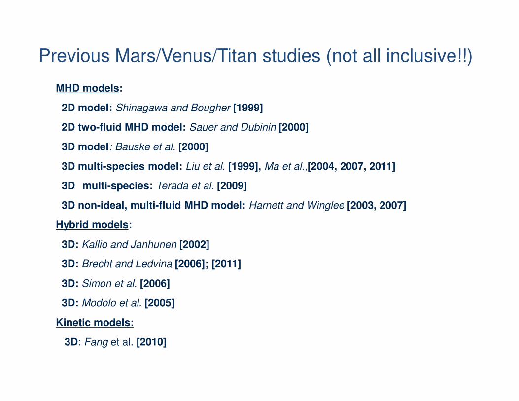
MHD models:

2D model: Shinagawa and Bougher [1999]

2D two-fluid MHD model: Sauer and Dubinin [2000]

3D model: Bauske et al. [2000]

3D multi-species model: Liu et al. [1999], Ma et al.,[2004, 2007, 2011]

3D multi-species: Terada et al. [2009]

3D non-ideal, multi-fluid MHD model: Harnett and Winglee [2003, 2007]

Previous Mars/Venus/Titan studies (not all inclusive!!)

3D non-ideal, multi-fluid MHD model: Harnett and Winglee [2003, 2007]

Hybrid models:

3D: Kallio and Janhunen [2002]

3D: Brecht and Ledvina [2006]; [2011]

3D: Simon et al. [2006]

3D: Modolo et al. [2005]

Kinetic models:

3D: Fang et al. [2010]

(neglecting resistive and Hall terms):

∂ρ s

∂t+ ∇. ρ su s( ) = Sρ

∂

∂tρi

4

∑

u

+ ∇ ⋅ ρi

4

∑

uu + p+

1

2B2

I − BB

= Sρu

∂ti

i=1

∑

i

i=1

∑

2

ρu

Že

Žt+ ∇. u e+p+

1

2B2

− B.u[ ]B

= Se

∂B

∂t− ∇ × u × B( )= 0

For each ion fluid, s, we obtain (neglecting resistive and Hall terms):

∂ρ s

∂t+ ∇. ρ su s( ) = Sρ

∂ρsus

∂t+ ∇. ρsusus + Ips( )= nsqs us − u+( )× B +

nsqs

n e(J × B − ∇pe )+ Sρs us

∂ps

∂t+ ∇. psus( )= − γ −1( )ps∇.us + Sp

∂B

∂t− ∇ × u+ × B( )= 0

∂t+ ∇. ρsusus + Ips( )= nsqs us − u+( )× B +

nee(J × B − ∇pe )+ Sρs us

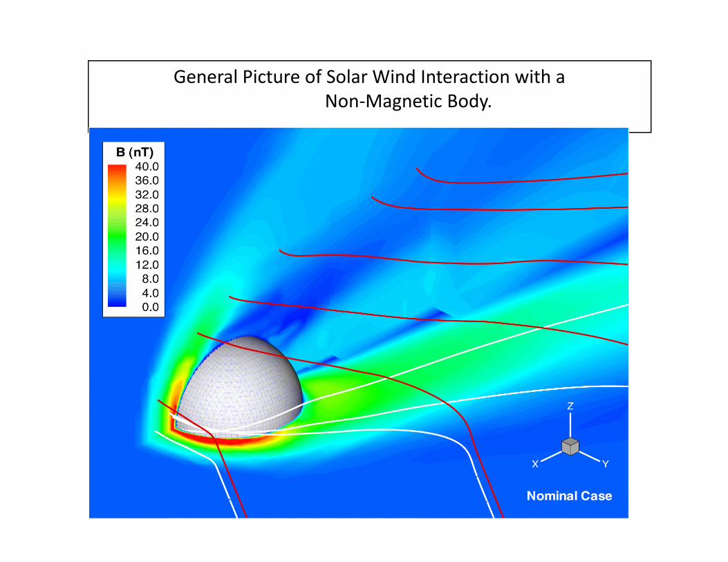
General Picture of Solar Wind Interaction with a

Non-Magnetic Body.

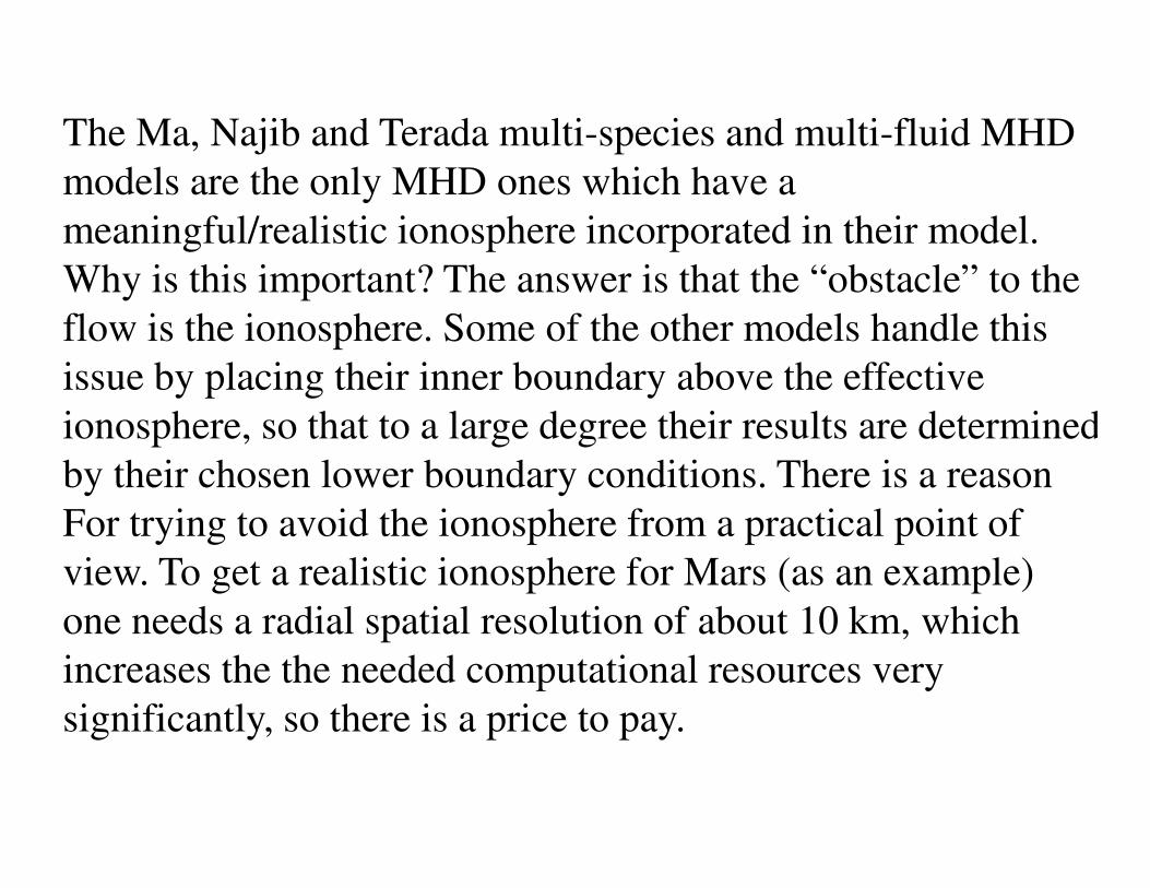
The Ma, Najib and Terada multi-species and multi-fluid MHD models are the only MHD ones which have a meaningful/realistic ionosphere incorporated in their model. Why is this important? The answer is that the “obstacle” to theflow is the ionosphere. Some of the other models handle thisissue by placing their inner boundary above the effective ionosphere, so that to a large degree their results are determinedionosphere, so that to a large degree their results are determinedby their chosen lower boundary conditions. There is a reason For trying to avoid the ionosphere from a practical point of view. To get a realistic ionosphere for Mars (as an example) one needs a radial spatial resolution of about 10 km, which increases the the needed computational resources very significantly, so there is a price to pay.

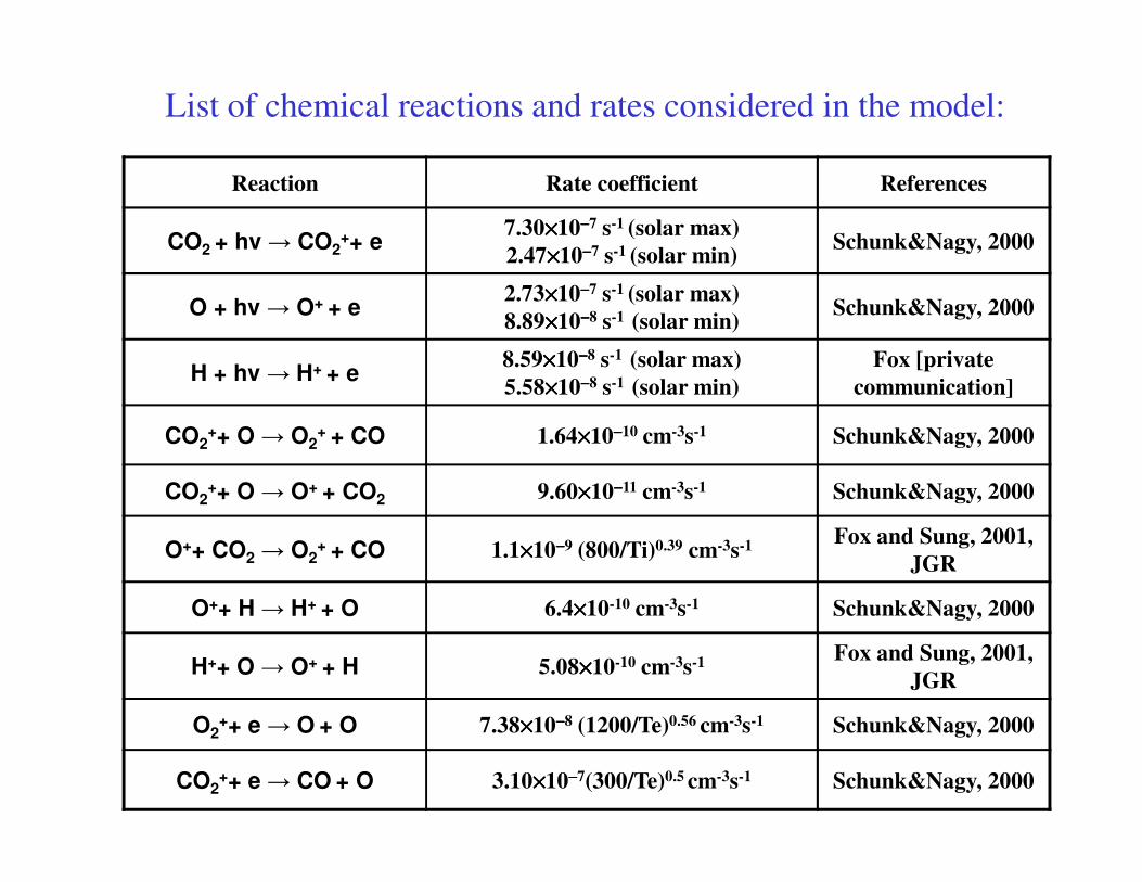
List of chemical reactions and rates considered in the model:

Reaction Rate coefficient References

CO2 + hv → CO2++ e

7.30××××10−−−−7 s-1 (solar max)

2.47××××10−−−−7 s-1 (solar min)Schunk&Nagy, 2000

O + hv → O+ + e2.73××××10−−−−7 s-1 (solar max)

8.89××××10−−−−8 s-1 (solar min)Schunk&Nagy, 2000

H + hv → H+ + e8.59××××10−−−−8 s-1 (solar max)

5.58××××10−−−−8 s-1 (solar min)

Fox [private

communication]

CO2++ O → O2

+ + CO 1.64××××10−−−−10 cm-3s-1 Schunk&Nagy, 2000CO2 + O → O2 + CO 1.64××××10 cm s Schunk&Nagy, 2000

CO2++ O → O+ + CO2 9.60××××10−−−−11 cm-3s-1 Schunk&Nagy, 2000

O++ CO2 → O2+ + CO 1.1××××10−−−−9 (800/Ti)0.39 cm-3s-1 Fox and Sung, 2001,

JGR

O++ H → H+ + O 6.4××××10-10 cm-3s-1 Schunk&Nagy, 2000

H++ O → O+ + H 5.08××××10-10 cm-3s-1 Fox and Sung, 2001,

JGR

O2++ e → O + O 7.38××××10−−−−8 (1200/Te)0.56 cm-3s-1 Schunk&Nagy, 2000

CO2++ e → CO + O 3.10××××10−−−−7(300/Te)0.5 cm-3s-1 Schunk&Nagy, 2000

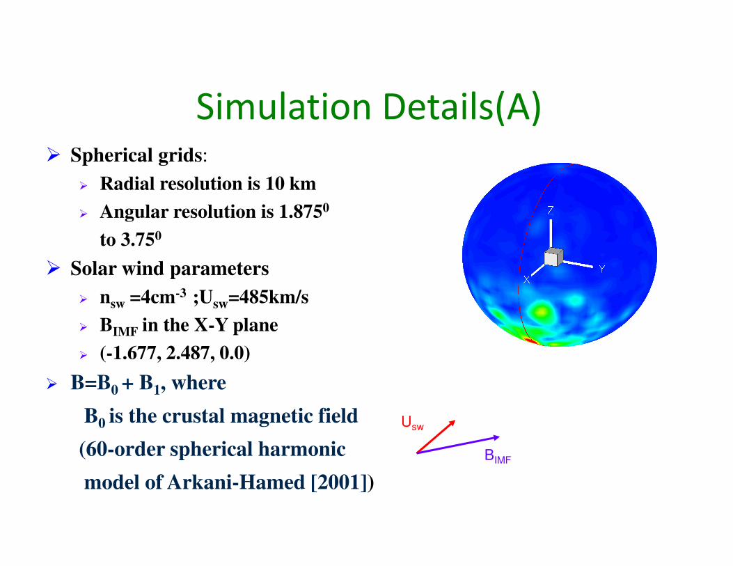
Simulation Details(A)� Spherical grids:

� Radial resolution is 10 km

� Angular resolution is 1.8750

to 3.750

� Solar wind parameters

� nsw =4cm-3 ;Usw=485km/s

� BIMF in the X-Y plane

� (-1.677, 2.487, 0.0)

� B=B0 + B1, where

B0 is the crustal magnetic field

(60-order spherical harmonic

model of Arkani-Hamed [2001])

Usw

BIMF

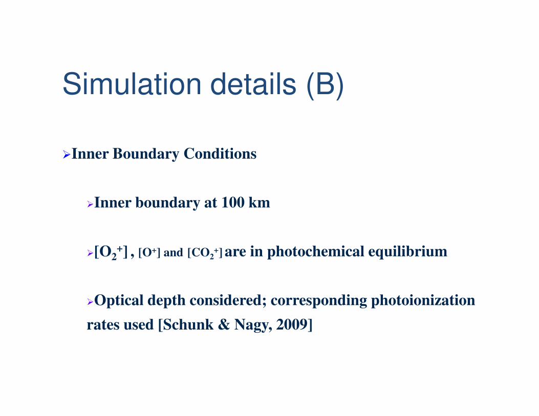
�Inner Boundary Conditions

�Inner boundary at 100 km

Simulation details (B)

�Inner boundary at 100 km

�[O2+] , [O+] and [CO2

+] are in photochemical equilibrium

�Optical depth considered; corresponding photoionization

rates used [Schunk & Nagy, 2009]

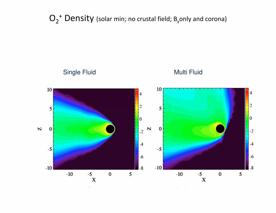
O2+ Density (solar min; no crustal field; Byonly and corona)

Single Fluid Multi Fluid

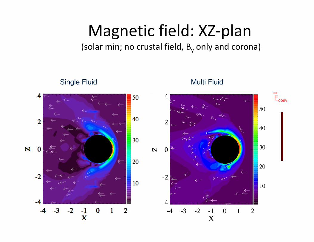
Magnetic field: XZ-plan(solar min; no crustal field, By only and corona)

Single Fluid Multi Fluid

Econv

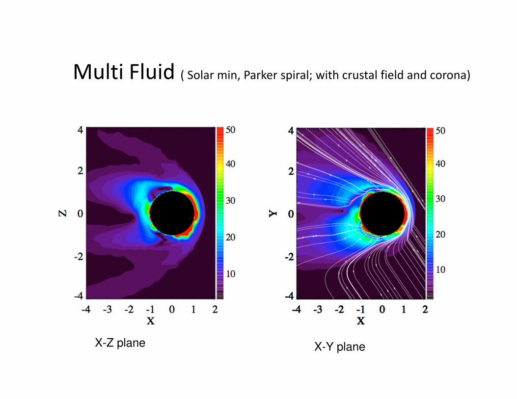
Multi Fluid ( Solar min, Parker spiral; with crustal field and corona)

X-Z plane X-Y plane

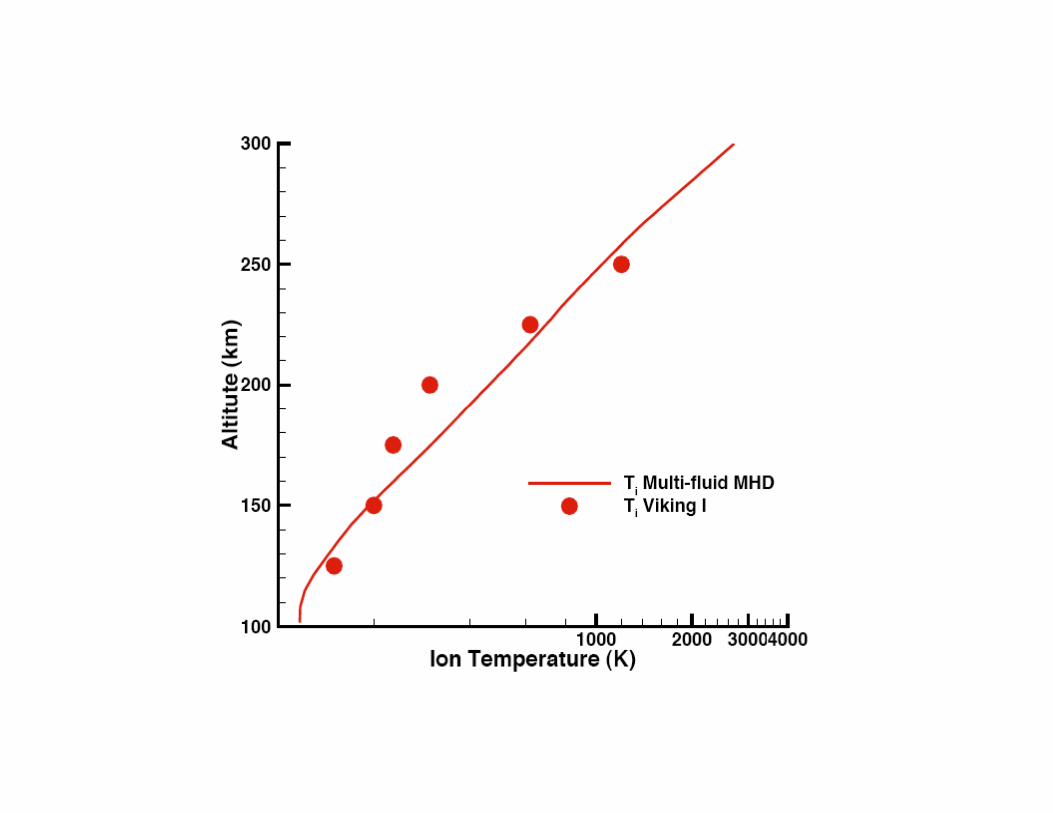
Pressure profiles along the Sun-Mars line for

solar maximum conditions.

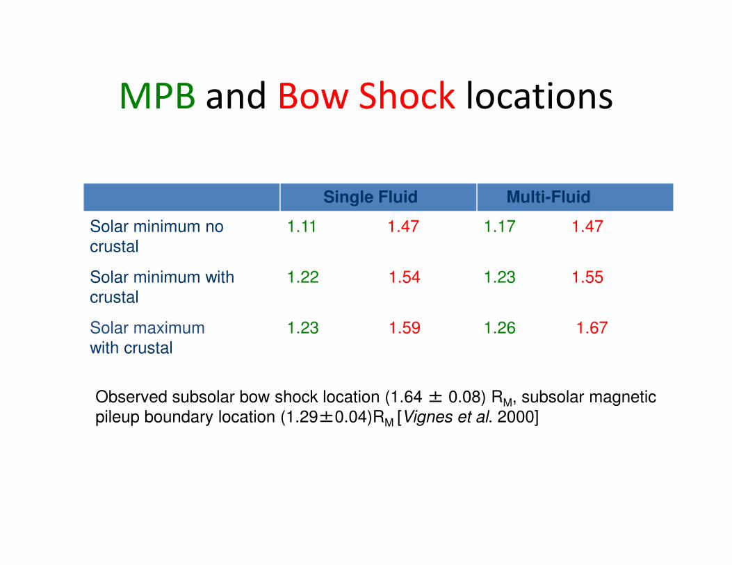
MPB and Bow Shock locations

Single Fluid Multi-Fluid

Solar minimum no

crustal

1.11 1.47 1.17 1.47

Solar minimum with 1.22 1.54 1.23 1.55Solar minimum with

crustal

1.22 1.54 1.23 1.55

Solar maximum

with crustal

1.23 1.59 1.26 1.67

Observed subsolar bow shock location (1.64 ± 0.08) RM, subsolar magnetic

pileup boundary location (1.29±0.04)RM [Vignes et al. 2000]

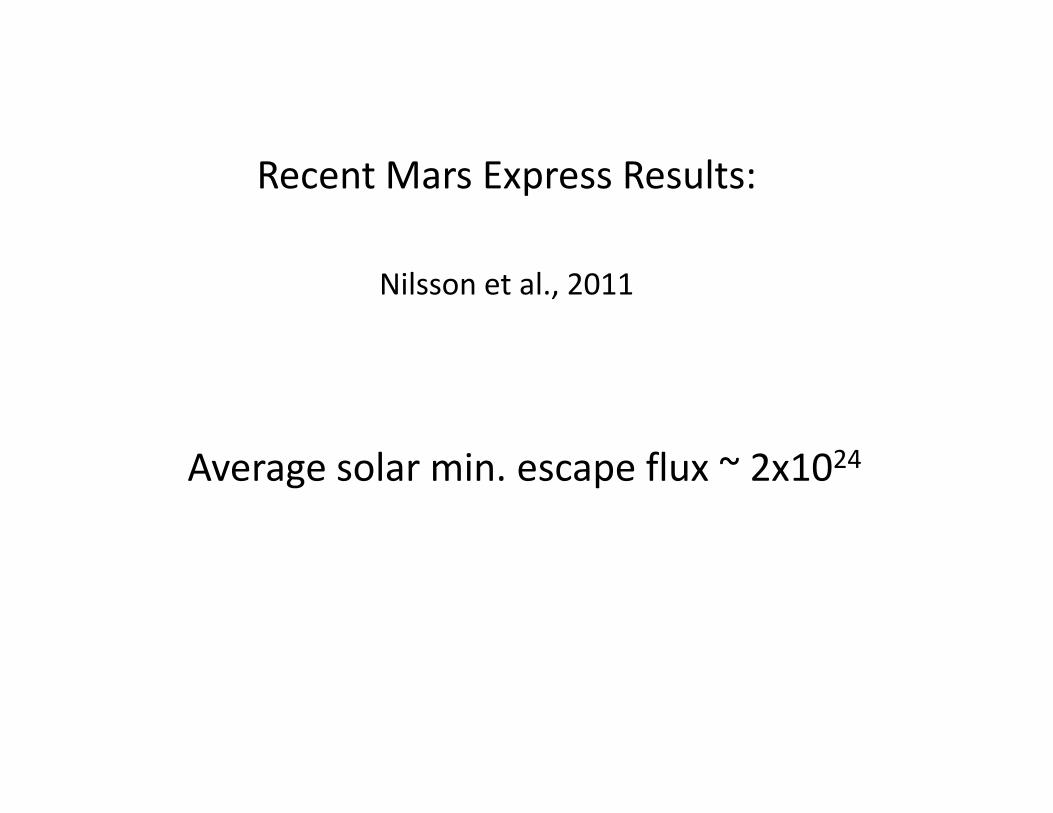
Recent Mars Express Results:

Nilsson et al., 2011

Average solar min. escape flux ~ 2x1024

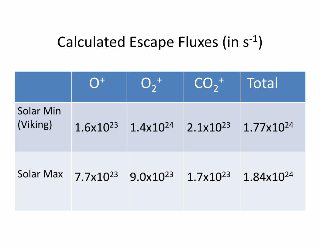
Calculated Escape Fluxes (in s-1)

O+ O2+ CO2

+ Total

Solar Min

(Viking) 1.6x1023 1.4x1024 2.1x1023 1.77x1024(Viking) 1.6x1023 1.4x1024 2.1x1023 1.77x1024

Solar Max 7.7x1023 9.0x1023 1.7x1023 1.84x1024

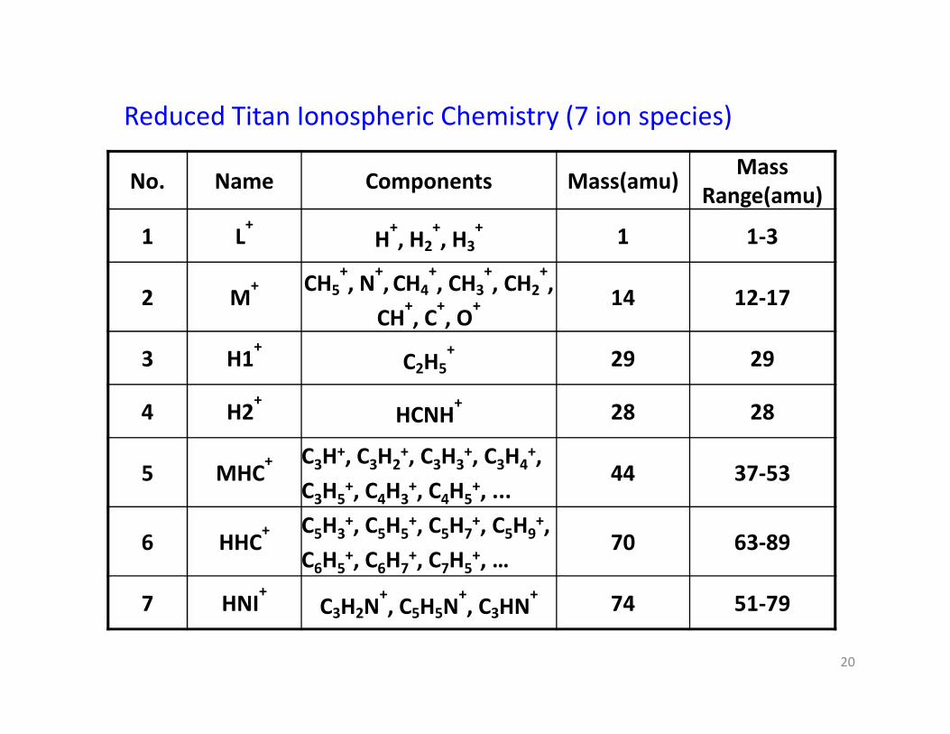
No. Name Components Mass(amu)Mass

Range(amu)

1 L+

H+, H2

+, H3

+1 1-3

2 M+ CH5

+, N

+, CH4

+, CH3

+, CH2

+,

CH+, C

+, O

+ 14 12-17

3 H1+

C2H5

+29 29

Reduced Titan Ionospheric Chemistry (7 ion species)

3 H1 C2H5 29 29

4 H2+

HCNH+

28 28

5 MHC+ C3H+, C3H2

+, C3H3+, C3H4

+,

C3H5+, C4H3

+, C4H5+, ...

44 37-53

6 HHC+ C5H3

+, C5H5+, C5H7

+, C5H9+,

C6H5+, C6H7

+, C7H5+, …

70 63-89

7 HNI+

C3H2N+, C5H5N

+, C3HN

+74 51-79

20

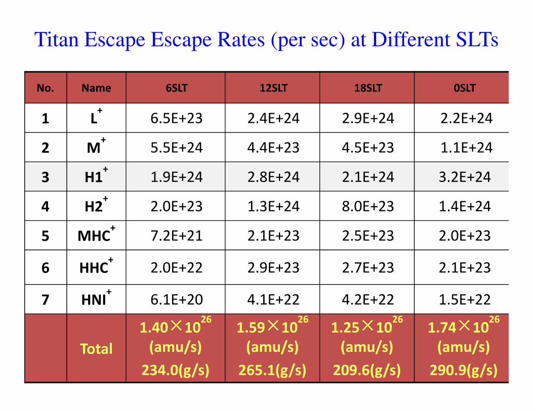
No. Name 6SLT 12SLT 18SLT 0SLT

1 L+

6.5E+23 2.4E+24 2.9E+24 2.2E+24

2 M+

5.5E+24 4.4E+23 4.5E+23 1.1E+24

3 H1+

1.9E+24 2.8E+24 2.1E+24 3.2E+24

4 H2+

2.0E+23 1.3E+24 8.0E+23 1.4E+24

Titan Escape Escape Rates (per sec) at Different SLTs

4 H2 2.0E+23 1.3E+24 8.0E+23 1.4E+24

5 MHC+

7.2E+21 2.1E+23 2.5E+23 2.0E+23

6 HHC+

2.0E+22 2.9E+23 2.7E+23 2.1E+23

7 HNI+

6.1E+20 4.1E+22 4.2E+22 1.5E+22

Total

1.40××××1026

(amu/s)

234.0(g/s)

1.59××××1026

(amu/s)

265.1(g/s)

1.25××××1026

(amu/s)

209.6(g/s)

1.74××××1026

(amu/s)

290.9(g/s)

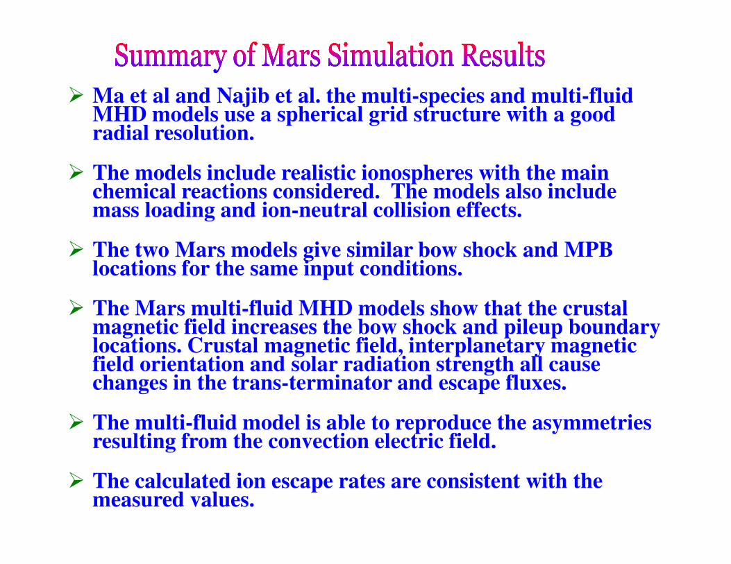
� Ma et al and Najib et al. the multi-species and multi-fluid MHD models use a spherical grid structure with a good radial resolution.

� The models include realistic ionospheres with the main chemical reactions considered. The models also include mass loading and ion-neutral collision effects.

� The two Mars models give similar bow shock and MPB locations for the same input conditions.

� The Mars multi-fluid MHD models show that the crustal magnetic field increases the bow shock and pileup boundary locations. Crustal magnetic field, interplanetary magnetic field orientation and solar radiation strength all cause changes in the trans-terminator and escape fluxes.

� The multi-fluid model is able to reproduce the asymmetries resulting from the convection electric field.

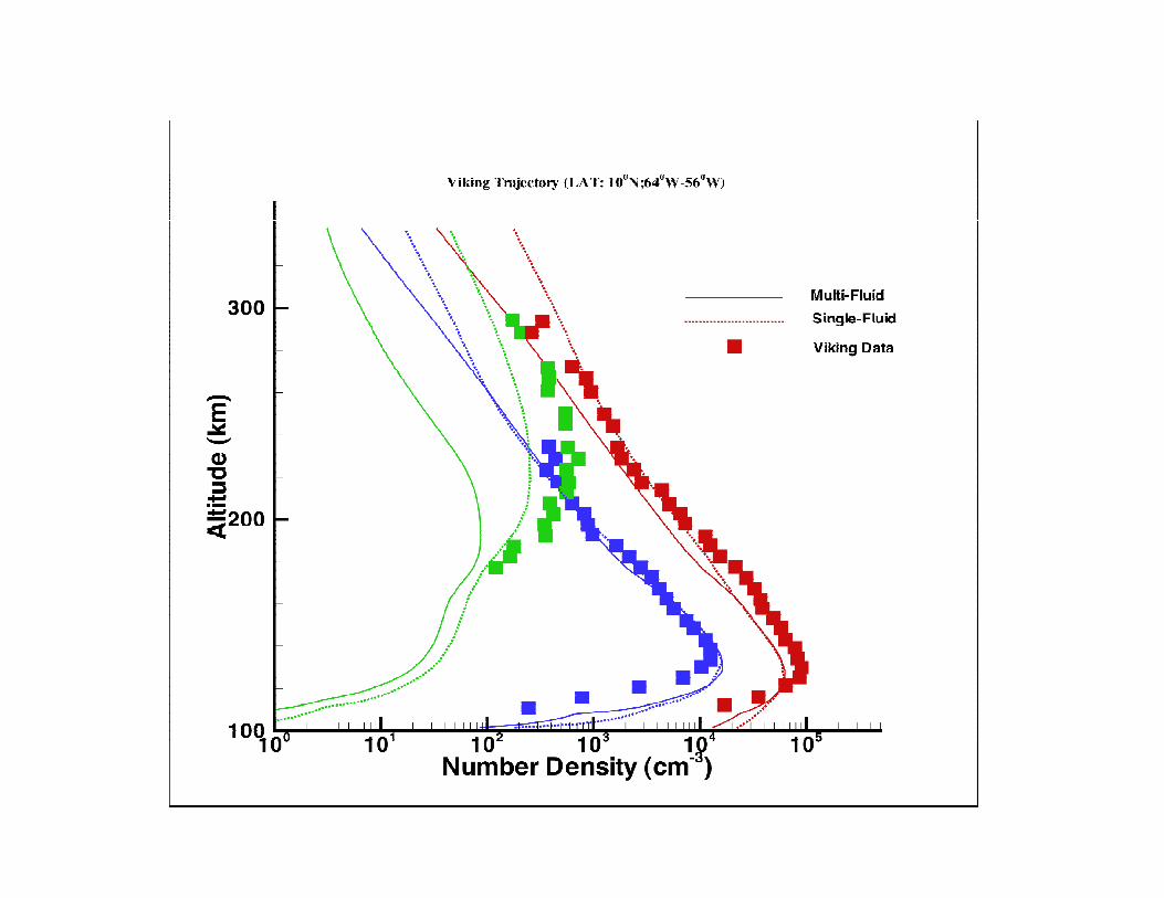
� The calculated ion escape rates are consistent with the measured values.