Liu, Park and Zheng

40

INTERNATIONAL REAL ESTATE REVIEW 2002 Vol. 5 No. 1: pp. 40 - 60

The Interaction between Housing Investment and Economic Growth in China Liu Hongyu, Institute of Real Estate Studies, Tsinghua University, Beijing 100084, China or liuhy@tsinghua.edu.cn Yun W. Park College of Business and Economics, California State University, 800 N. State College Blvd., Fullerton, CA 92834-6848 or yunpark@fullerton.edu Zheng Siqi, Institute of Real Estate Studies, Tsinghua University, Beijing 100084, China or zhengsq00@mails.tsinghua.edu.cn The importance of housing investment in the national economy and its rapid growth have become distinct characteristics of the Chinese economy in recent years. However, at the same time, there is a concern that the economic growth heavily dependent on housing investment may compromise the stability and the health of the national economy. Using Granger causality analysis, this paper examines the interaction between housing investment and economic growth as well as that between non-housing investment and economic growth. We find evidence that housing investment has a stronger short run effect on economic growth than non-housing investment. We also find that housing investment has a long run effect on economic growth while economic growth has a log run effect on both housing and non-housing investment. Our findings suggest that housing investment is an important factor for the short-term fluctuations of economic growth, with its growth stimulating the economic growth and its slumps leading to downside fluctuations. Keywords Economic growth, housing investment, non-housing investment, Granger causality, cointegration, error correction model

The Interaction between Housing Investment and Economic Growth

41

Introduction The high growth rate the Chinese economy has achieved in recent years is unusual, especially in view of the generally weak economy around the world. The Chinese government has consistently emphasized the role of aggregate investment in stimulating the growth of the national economy. This government policy appears to have produced the intended outcome. According to the Chinese Academy of International Trade and Economic Cooperation (2002), on average investment accounts for about 4% in the growth rates of gross domestic products (GDP) for the 1998-2002 period, which average about 8%. This translates to more than 50% of the total growth rate and exceeds the contributions of consumption and net exports, which account for about 3% and 1%, respectively. Of the different types of investment, housing investment increased unusually fast in this period due at least in part to two reasons1. One factor is the housing reform in 1998, which made the free market the main channel for the provision of residential housing. The housing reform of 1998 unleashed a huge demand for housing and the potential for high profits encouraged real estate developers to construct more and more houses. The second factor is the government blessing for real estate development. In an attempt to achieve a high GDP growth rate, the Chinese government encouraged housing construction. There are anecdotal evidences that the bureau in charge of housing investment relaxed standards of examination and approval and that banks provided easy credit for housing development projects. As a result, commercial housing investment, which emerged as a viable alternative to government housing investment, has reached a very high growth rate in recent years. According to the National Bureau of Statistics of China (2002), housing growth rates were 35.2%, 26.8%, 25.5% and 27.3% in 1998, 1999, 2000 and 2001, respectively. Since commercial housing investment is the largest and the most important segment in real estate development investment in China, its rapid growth inevitably lead to a high growth rate of real estate investment. The Monetary Policy Analysis Group of People’s Bank of China (2002) reports that, of the GDP growth rate of 7.3% in 2001, 1.3 percent was directly contributed by the real estate sector and 1.9-2.5% was directly or indirectly contributed by the real estate sector. This implies that the real estate sector accounted for 30% of the GDP growth rate in 2001.

1 See Liu (1998) for a comprehensive survey of the real estate market in China as well as the role of government policies in housing development.

Liu, Park and Zheng

42

In order to formally assess the impact of housing investment on the national economy in China, we investigate the short run as well as the long run effect of housing investment on the determination of economic growth using appropriate macro time series. We also compare it with the effect of non-housing investment on the national output. Economic theory indicates that real estate development decoupled from the larger economic development will be corrected in the long run. Equilibrium considerations suggest that the development of the real estate market cannot be sustained without corresponding economic growth in the long run. Therefore, we investigate whether the long run behavior of housing investment is guided by the long run behavior of GDP. In short, this study investigates the short run and the long run dynamic relationships between housing investment and economic growth as well as those between non-housing investment and economic growth and compares the nature of these relationships. Some unique institutional settings of the Chinese real estate market discussed earlier in the introduction make the findings of this research particularly valuable. The Chinese real estate market represents a unique natural experiment in that both the macro economy and the real estate market in China are in the early stage of development after emerging from the long period of planned economy. In part because of the short macro time series available, virtually no carefully conducted econometric study exists in the literature which examines the macro-economic relevance of the Chinese real estate market. The remainder of the article is organized as follows. Section 2 reviews the relevant literature. Section 3 discusses the methodology and empirical models used in this study. The data are described in Section 4. The results are explained in Section 5. Finally, the conclusions and policy implications are presented in Section 6. Literature Review A considerable volume of literature exists that investigates the dynamic interactions of GDP and housing investment. A number of economists have maintained that subsidizing housing investment leads to a serious misallocation of capital2. In support of this view, Mills (1987) documents that the return to housing capital is about half that to non-housing capital. More recently, using a pooled cross section and time-series analysis of 18

2 See Mills (1987) for a review.

The Interaction between Housing Investment and Economic Growth

43

OECD countries over the period from 1950 to 1999, Madsen (2002) revisits the causality between investment and economic growth. On the basis of the findings that growth is predominantly caused by investment in machinery and equipment, he suggests that policies that seek to enhance investment in equipment and machinery are effective means of promoting economic growth. On the other hand, others argue that the external benefits associated with housing investment could justify the subsidy on housing investment at least in part. One of the benefits of housing investment is that it may stimulate the economy. Indeed, it may stimulate the GDP growth more than the other types of investment. Using the U.S. data, Green (1997) finds that under a wide variety of time-series specifications, housing investment causes the growth of GDP, but is not caused by it, while non-housing investment does not cause the growth of GDP, but is caused by it. He observes that housing leads and other types of investment lag the business cycle. He argues that his results suggest that policies should be designed to avoid channeling capital away from housing into plant and equipment sectors, or severe short run dislocations may occur. Coulson and Kim (2000) observe that Green (1997) does not consider the influences that components of GDP other than housing investment might have on it when trying to assess the importance of housing investment in the determination of GDP. In an attempt to remedy this deficiency, they use multivariate vector autoregression models to test the influence of housing and non-housing investment on GDP and its components. Their finding that housing investment shocks are more important in the determination of GDP than non-housing investment is consistent with that of Green (1997). Chau and Zou (2000) investigate the short run as well as the long run effects of both public and private housing investment on GDP in Hong Kong from 1973 to 1999. They report that while the growth in public housing investment has a positive influence on the long run economic growth, private housing investment is influential in determining short run economic output. More recently, Wen (2001) points out that differentiating residential investment from business investment is important in analyzing the relationship between capital formation and economic growth noting that the majority of household savings are in the form of real estate and that economic booms often follow real estate booms and economic recessions follow real estate slumps. Using the postwar U.S. data, Wen shows that it is the capital formation in the household sector that unambiguously and unilaterally causes GDP growth, which in turn causes capital formation in the business sector.

Liu, Park and Zheng

44

The finding that housing investment has an important short run influence on GDP in the economies of Hong Kong and the U.S. may be widely observed. This study investigates the short-term effect of housing investment on GDP using the Chinese data. Furthermore, some Hong Kong and U.S. studies report a surprising result that non-housing investment has no or less discernible short-term effect on GDP. This study also investigates the short run effect of non-housing investment on GDP using the Chinese data. Equilibrium considerations suggest that GDP must provide long run guidance to both housing and non-housing investments. Furthermore, Leung (2003) develops a model, in which a persistent economic growth has a long run effect on housing prices. Leung shows that a long-term increase in housing prices can result from a persistent economic growth and suggests that persistent price run-ups recently observed in several cities and countries in Asia and North America may be due to the persistent economic growth in these regions. On the other hand, Brito and Perreira (2002) develop a model, in which housing investment and non-housing investment have a long run effect on economic growth. Brito and Perreira, using an endogenous growth model where housing plays a role as a consumption and an investment good for households as well as an input to production for the production sector, show that productivity shocks to manufacturing, construction, and educational and training activities have positive effects on long-term growth and that for reasonable parameter values the responsiveness of the long term growth rate to shocks to construction is greater than its responsiveness to shocks in manufacturing. However, the existing literature does not provide conclusive empirical evidence on the issue of long run relationship between housing and non-housing investment and economic growth. To understand this issue better, we explicitly examine the long-term interaction among GDP, housing investment and non-housing investment. Methodology In order to explore the causal relationships between housing investment and GDP, the widely accepted Granger causality method is used throughout. To implement the Granger test, we assume a particular autoregressive lag length and estimate vector autoregression (VAR) models by the ordinary least squares (OLS) estimation method. If the time series are not stationary but integrated of the first order, they should be differenced to become stationary.

The Interaction between Housing Investment and Economic Growth

45

In the absence of cointegration, we may formulate the models in terms of the first differences as in equations (1) and (2):

∑∑=

−=

− +∆+∆+=∆k

jtjtj

k

iitit YbXaX

1,1,1

1,11 µλ (1)

∑∑=

−=

− +∆+∆+=∆p

jtjtj

p

iitit YbXaY

1,2,2

1,22 µλ (2)

Following Toda and Phillips (1993) and Hamilton (1994, p.304-306), we use the Wald χ2 test to test for the null hypothesis of no short run effect in the absence of cointegration between X and Y. Following Engle and Granger (1987), if two series {Xt} and {Yt} are each integrated of order one but are also co-integrated, we estimate the following error-correction models (ECM):

tt

k

jjtj

k

iitit ECYXX ,11,11

1,1

1,11 µφβαλ ++∆+∆+=∆ −

=−

=− ∑∑ ,where

11,1 )( −− −= tt YXEC γ (3)

t

k

jtjtj

k

iitit ECYXY ,2

11,22,2

1,22 µφβαλ ++∆+∆+=∆ ∑∑

=−−

=−

, where 11,2 )( −− −= tt XYEC δ (4)

1, −tiEC (i=1, 2) is the error-correction term, which is related to the long run

equilibrium between variables. The error correction term is calculated as residuals of the cointegration equations. In Equations (3) and (4), all series are I(0) processes. 1φ and

2φ are called coefficients of adjustment. 1φ , the coefficient of

1,1 −tEC , is the long run elasticity of X with respect to Y. Similarly, 2φ , the

coefficient of 1,2 −tEC , is the long run elasticity of Y with respect to X. We

use the t-statistic of the coefficient of adjustment to test for the long term effect. On the other hand,

j,1β and i,2α reflect the immediate response of X

to changes in Y and that of Y to changes in X, respectively. They are, therefore, the short run elasticities. Following Toda and Phillips (1994), we also use the Wald 2χ statistic to test for the null hypothesis that short run causality does not exist. We use the augmented Dickey-Fuller (ADF) method to test the order of the series, and Johansen’s method to test whether a cointegrating relationship exists between the series.

Liu, Park and Zheng

46

Data The available data of GDP and housing investment in China date from 1981. Before the 1980 reform of National Economic Statistics System in 1981, the National Bureau of Statistics of China reported GNP rather than GDP. The annual time series of GDP along with housing and non-housing investment for the 1981-2000 period are constructed on the basis of the data collected from the relevant issues of China Statistics yearbooks. In the following empirical study, GDP, housing investment (HI) and non-housing investment (NI) are expressed in reference to the constant market prices of 1981. The weights of housing investment in GDP varied from 6.1% to 8.6%, with the average of 7.4% and standard deviation of 0.8%. Figure 1 shows the fluctuations of the importance of housing investment from 1981 to 2000. The relative importance of the housing sector in the national economy has remained reasonably constant during the period while showing cyclical variations. Reflecting the recent boom in the real estate market, it rises above 8.0% after 1998. Figure 1. Weight of Housing Investment (HI) in GDP

Table 1 Comparison of Housing Investment and GDP in the United States and China in

2000

United States China GDP (in US$ millions) 9872.9 1077.2 Private domestic investment (in US$ millions) 1718.1 376.2

Housing investment (in US$ millions) 425.1 91.5

0

2

4

6

8

10

12

1981 1983 1985 1987 1989 1991 1993 1995 1997 1999

Year

HI/G

DP

(%)

The Interaction between Housing Investment and Economic Growth

47

Housing investment in GDP (%) 4.3 8.5 Housing investment in private domestic investment (%) 24.7 24.3

Notes: GDP, private domestic investment and housing investment are in 2000 U.S dollars.

Table 1 gives the comparison of housing investment and GDP between the United States and China in the year 2000. While the weight of housing investment in GDP in China is much larger than that in the United States, the weight of housing investment in private domestic investment is similar to that in the United States. The larger weight of housing investment, which reflects the fact that the housing construction sector is under vigorous development in China, suggests a potential overdependence of the national economy on housing investment. This study uses annual time series. The econometrical analysis is conducted under the constraint of a small sample size. Quarterly data cannot be used in this study because the National Bureau of Statistics of China began to report quarterly GDP only from 1997. Furthermore, while quarterly data exist for some portions of housing investment, the quality of the quarterly housing investment data is suspect. Their measurement is by and large coarse and the statistical methods and the boundary of the measures used have changed substantially during this period. While the number of observations is relatively short (N=20), the time series data extend over a meaningfully long period (20 years). More importantly, this time series covers the entire period of the market experiment in China. Often it is convenient to explore the long run relationships between economic series in terms of their rates of change. If the change in a variable is relatively small, the first difference of the logarithms of the variable is approximately equal to the rate of change because:

1

1

11 )()()(

−

−

−−

−≈=−

t

tt

t

ttt X

XXXX

LnXLnXLn (5)

For this reason, the annual time series of GDP, housing investment (HI) and non-housing investment (NI) measured in the constant market prices of 1981 are transformed into their natural logarithms.

Liu, Park and Zheng

48

Empirical Results Unit Root Tests of the Stationary of Time Series Using the augmented Dickey-Fuller (ADF) test, we formally test whether Ln(GDP), Ln(HI) and Ln(NI) are I(1). The augmented Dickey-Fuller test regresses the change in the indicated variable on its lagged variable in level and on its lagged differences. The optimal lag length of the lagged differences of the tested variable is determined by minimizing the Akaike Information Criteria (AIC). The maximum lag length is set at three years in all tests following the suggestion from Wooldridge (1999, p. 582) who recommends one or two years of leg length for annual data, and in view of the fact that the Chinese times series used are relatively short. Furthermore, by minimizing the Akaike Information Criteria (AIC), we find it optimal to include an intercept, but exclude the linear trend variable for all regression equations. If the test statistic of the level term, which is known as the ADF test statistic, is less than the critical value, then the null hypothesis of integratedness is rejected. Panel A of Table 2 shows that the ADF test statistics of Ln(GDP), Ln(HI) as well as Ln(NI) are greater than the 5% critical value indicating that the coefficients of the lagged level terms of Ln(GDP), Ln(HI), and Ln(NI) are not significantly different from zero. It is inferred that Ln(GDP), Ln(HI), and Ln(NI) are essentially unit root processes and approximately I(1). Note that the ADF test statistic does not have the usual t-distribution. On the other hand, the augmented Dickey-Fuller tests shown in Panel B suggest that the first differences of Ln(GDP), Ln(HI) and Ln(NI) denoted as ∆Ln(GDP), ∆Ln(HI), and ∆Ln(NI), respectively, are all stationary series, i.e., I(0). The results of the Augmented Dickey-Fuller (ADF) tests in Panels A and B strongly suggest that Ln(GDP), Ln(HI), and Ln(NI) can be approximated by I(1) process. Table 2: Augmented Dickey-Fuller Unit Root Tests of the Stationarity of Time Series Panel A. Tests of the Stationarity of the Levels of Time Series

Time Series Variable

Included in the Test Equation

Leg Length

ADF Test Statistics

Inferred Order of

Integratedness Ln GDP Intercept 3 -1.099

(-3.052) I(1)

The Interaction between Housing Investment and Economic Growth

49

Ln HI Intercept 3 -0.936 (-3.030)

I(1)

Ln NI Intercept 2 -1.251 (-3.052)

I(1)

Panel B. Tests of the Stationarity of the Fist Differences of Time Series

Time Series Variable

Included in the Test Equation

Leg Length

ADF Test

Statistics

Inferred Order of Integratedness

∆Ln GDP Intercept 3 -3.215* (-3.082)

I(0)

∆Ln HI Intercept 3 -4.210* (-3.082)

I(0)

∆Ln NI Intercept 2 -3.395* (-3.066)

I(0)

Notes: Ln GDP, Ln HI, and Ln NI are the natural logarithms of GDP, housing investment and non-housing investment, respectively. All series are in 1981 constant prices. ∆Ln GDP, ∆Ln HI, and ∆Ln NI are the first differences of Ln GDP, Ln HI and Ln NI, respectively. The 5% confidence level is shown in parenthesis below the ADF test statistics. The asterisk indicates significance at the 5% level. Note that the distribution of the ADF test statistics is not the usual t-distribution. Finally, the order of integratedness of the indicated time series inferred from the ADF tests is shown in the last column. Results of the Cointegration Tests For a cointegrated pair of variables it is important to distinguish long run from short run interactions. With this in mind, we conduct tests of cointegration using Johansen’s methodology (1991). The Johansen test estimates a bivariate vector autoregression model using differences of the indicated variables as the dependent variables, and a lagged level term for each variable, along with lagged differences as explanatory variables. In addition, we include an intercept, but exclude the trend variable for both VAR equations and cointegration equations. The optimal lag length is determined by minimizing the Akaike Information Criteria (AIC). If the matrix of the coefficients of the level terms is of less than the full rank of two, there is a common long run relationship between the two variables, i.e., co-integration. The Johansen test is a test of the rank of this matrix, and a test statistic greater than the critical value indicates the rejection of the hypothesis of full rank. The log likelihood (LR) test statistic tests the null hypothesis of no cointegration. Table 3 reports the test results. Two cointegrating relationships are detected. The null hypothesis of no cointegration is rejected at the 5% level of significance for the Ln(GNP) and Ln(HI) pair as well as the Ln(GNP) and

Liu, Park and Zheng

50

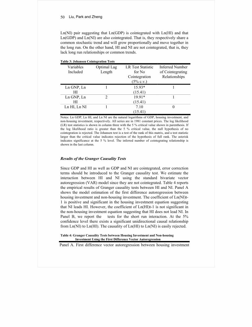
Ln(NI) pair suggesting that Ln(GDP) is cointegrated with Ln(HI) and that Ln(GDP) and Ln(NI) are also cointegrated. That is, they respectively share a common stochastic trend and will grow proportionally and move together in the long run. On the other hand, HI and NI are not cointegrated, that is, they lack long run relationships or common trends. Table 3: Johansen Cointegration Tests

Variables Included

Optimal Lag Length

LR Test Statistic for No

Cointegration (5% c.v.)

Inferred Number of Cointegrating

Relationships

Ln GNP, Ln HI

1

15.93* (15.41)

1

Ln GNP, Ln HI

2

19.91* (15.41)

1

Ln HI, Ln NI 1

7.10 (15.41)

0

Notes: Ln GDP, Ln HI, and Ln NI are the natural logarithms of GDP, housing investment, and non-housing investment, respectively. All series are in 1981 constant prices. The log likelihood (LR) test statistics is shown in column three with the 5 % critical value shown in parenthesis. If the log likelihood ratio is greater than the 5 % critical value, the null hypothesis of no cointegration is rejected. The Johansen test is a test of the rank of this matrix, and a test statistic larger than the critical value indicates rejection of the hypothesis of full rank. The asterisk indicates significance at the 5 % level. The inferred number of cointegrating relationship is shown in the last column. Results of the Granger Causality Tests Since GDP and HI as well as GDP and NI are cointegrated, error correction terms should be introduced to the Granger causality test. We estimate the interaction between HI and NI using the standard bivariate vector autoregression (VAR) model since they are not cointegrated. Table 4 reports the empirical results of Granger causality tests between HI and NI. Panel A shows the model estimation of the first difference autoregression between housing investment and non-housing investment. The coefficient of Ln(NI)t-1 is positive and significant in the housing investment equation suggesting that NI leads HI. However, the coefficient of Ln(HI)t-1 is not significant in the non-housing investment equation suggesting that HI does not lead NI. In Panel B, we report the tests for the short run interaction. At the 5% confidence level there exists a significant unidirectional causal relationship from Ln(NI) to Ln(HI). The causality of Ln(HI) to Ln(NI) is easily rejected. Table 4: Granger Causality Tests between Housing Investment and Non-housing

Investment Using the First Difference Vector Autoregression

Panel A. First difference vector autoregression between housing investment

The Interaction between Housing Investment and Economic Growth

51

and non-housing investment Dependent Variable ∆Ln(HI)t ∆Ln(NI)t

Intercept 0.055* (2.387)

0.077 (0.071)

∆Ln(HI)t-1 -0.675* (-2.560)

-0.758 (-1.642)

∆Ln(NI)t-1 0.907*

(4.632) 0.932* (0.016)

R squares 0.629 0.356 Adjusted R squares 0.580 0.271

Panel B. Granger causality tests Null Hypothesis: 2χ statistic P-value

Ln(NI) does not Granger CauseLn(HI)

21.452* 0.000

Ln(HI) does not Granger Cause Ln(NI)

2.697 0.101

Notes: Ln(GDP), Ln(HI), and Ln(NI) are the natural logarithms of GDP, housing investment, and non-housing investment, respectively. All series are in 1981 constant prices. ∆Ln(GDP), ∆Ln(HI), and ∆Ln(NI) are the first differences of Ln(GDP), Ln(HI) and Ln(NI), respectively. In Panel A t-statistics of estimated coefficients are reported in parenthesis. The lag length of one is from the cointegration analysis reported in Table 3. The second column of Panel B shows the χ2 tests of the null hypothesis that the lag coefficient of the causal variable is equal to zero. The asterisk indicates rejection of the null hypothesis at the 5% level of significance. Next, the short run and the long run interactions between Ln(GDP) and Ln(HI) as well as Ln(GDP) and Ln(NI) are investigated. Table 5 reports the Granger causality tests using error correction models. Based on the cointegration test results in Table 3, we obtain the cointegrating vector, and then we construct the ECM models by fitting the vector of residuals into the standard VAR models as error correction terms. Optimal lag lengths are chosen using the Akaike information criteria (AIC). Table 5 shows that the coefficient of the EC term in the equation testing for the causality from Ln(GDP) to Ln(HI) as well as the coefficient of the EC term in the equation testing for the causality from Ln(HI) to Ln(GDP) is significant at the 5% confidence level. This result suggests the existence of a bidirectional long run relationship between GDP to HI. The coefficient of the EC term in the equation studying the long run effect of Ln(GDP) on Ln(NI) is also significant at the 5% confidence level, suggesting that GDP is a long-term determinant on non-housing investment as well.

Liu, Park and Zheng

52

Table 5. Granger Causality Tests for the Interaction of GDP and HI, and GDP and NI Using Vector Error-correction

Notes: Ln(GDP), Ln(HI), and Ln(NI) are the natural logarithms of GDP, housing investment, and non-housing investment, respectively. All series are in 1981 constant prices. ∆Ln(GDP), ∆Ln(HI), and ∆Ln(NI) are the first differences of Ln(GDP), Ln(HI), and Ln(NI), respectively. ECM 1 (the error correction model one) models the interaction between GDP and housing investment. ECM 2 (the error correction model one) models the interaction between GDP and non-housing investment. T-statistics of estimated coefficients are reported in parenthesis. The lag length used is from the cointegration analysis reported in Table 3. The asterisk indicates significance at the 5 % level. The p-values of the χ2 statistics are shown in square brackets. The short run interactions are investigated using the t-statistics of lagged explanatory variables. We also use the Wald statistic for the null hypothesis that short run causality does not exist. The coefficient of ∆Ln(HI)t-1 in the GDP equation in ECM 1 is positive and significant suggesting that housing investment leads GDP by one year. However, the coefficients of both ∆Ln(NI)t-1 and ∆Ln(NI)t-2 in the GDP equation in ECM 2 are not

ECM 1 ECM 2

Dependent variables ∆Ln(GDP)t ∆Ln(HI)t ∆Ln(GDP)t ∆Ln(NI)t Intercept 0.044* -0.059 0.104* -0.003 (2.026) (-0.816) (2.474) (-0.014) EC 0.132* 0.842* 0.030 1.199*

(2.048) (3.904) (0.301) (2.845) ∆Ln(GDP)t-1 0.382 -1.979 0.225 -0.206 (1.527) (-1.324) (0.597) (-0.127) ∆Ln(GDP)t-2 -0.541 -0.063 (-1.511) (-0.041) ∆Ln(HI)t-1 0.142* 1.532* (2.027) (2.268) ∆Ln(NI)t-1 0.095 0.909*

(1.376) (3.061) ∆Ln(NI)t-2 0.085 0.295 (1.212) (0.983) Wald 2χ for H0 4.107* 1.608 4.010 0.021

[0.04] [0.21] [0.14] [0.99]

The Interaction between Housing Investment and Economic Growth

53

significant suggesting that non-housing investment does not lead GDP either by one year or two years. Not surprisingly, the statistic of the GDP equation in ECM 1 is significant at the 5% level indicating that the short run effect of housing investment on GDP is significant. On the other hand, the statistic of the GDP equation in ECM 2 is significant only at the 15% level providing at most a weak evidence of the short run effect of non-housing investment on GDP. Both the t-statistics of the lagged explanatory variables and the statistics suggest that the short run effect of housing investment on economic growth is clearly stronger than that of non-housing investment. In summary, housing investment has a short run influence on GDP and not vice versa, while there is only a weak evidence of a short run effect of non-housing investment on GDP. In addition, non-housing investment has a short run effect on housing investment. Housing investment has a long run influence on GDP whereas non-housing investment does not. GDP has a long run influence on both housing investment and non-housing investment. There is a long run feedback relationship between GDP and housing investment, but not between GDP and non-housing investment. Our short run results, which suggest the dominant short run effect of housing investment on economic growth, are largely consistent with those of Green (1997), Coulsen and Kim (2000), Chau and Zou (2000) and Wen (2001) among others. At the same time, they are inconsistent with Mills (1987) and Madsen (2002) among others, who show that non-housing investment is more important to economic growth than housing investment. Our long run results, which suggest a long run effect of housing investment on economic growth, are consistent with the theoretical predictions of Brito and Perreira (2002) while the long run effect of economic growth on housing and non-housing investment is consistent with the general equilibrium arguments as well as Leung (2003) among others. Finally, the bi-directional long run relationship between housing investment and economic growth is consistent with the theoretical predictions of Zhang (1994, 1998) among others. Robustness Tests Neely and Weller (2000) demonstrate that the conventional VAR results could be misleading if the times series possess a structural change. Therefore, we check the structural stability of the parameters in equations (1)-(4) using cusum (standardized cumulative recursive residuals) tests and cusum of square tests. Plots of both cusum test statistics and cusum of square test statistics for all four equations, which are not reported as figures, remain

Liu, Park and Zheng

54

essentially within their 5 % critical lines suggesting that a regime shift does not occur during the sample period. As a further robustness check, we control for the effect of the Asian financial crisis and then the effect of the Chinese housing reform in models that examine the interaction of housing investment and GDP. We find that the documented relationship between housing investment and GDP as well as non-housing investment and GDP persists. Table 6 reports the effect of the Asian financial crisis on the model estimation. AFC is a dummy variable for the Asian financial crisis. It takes the value of one for years 1997, 1998, and 1999 and zero otherwise. The statistic of the equation of GDP as a function of HI in ECM 1 is significant confirming the short run effect of housing investment on GDP. The absence of a short term effect of non-housing investment on GDP is also persistent for the statistic of the equation of GDP as a function of NI in ECM 2 is insignificant. Both the coefficient of the error correction term (EC) in the housing investment equation of ECM 1 and that in the non-housing investment equation of ECM 2 are positive and significant confirming the long run influence of GDP on both housing and non-housing investments even when the Asian financial crisis is controlled for. The coefficient of the Asian financial crisis dummy (AFC) is not significant at the conventional level suggesting that the Chinese economy and its real estate market were not affected by the Asian financial crisis. While not reported as a table, the models that include interaction terms between AFC and the proposed causal terms are estimated. The coefficients of these interaction terms are not significant suggesting that the slopes of proposed causal variables were not affected by the Asian financial crisis. Table 7 reports the effect of Chinese housing reform on the model estimation. CHR is a dummy variable for the Chinese housing reform. It takes the value of one for years later than 1997 and zero otherwise. The statistics of the equation of GDP as a function of HI in ECM 1 confirms the short run effect of housing investment on GDP. However, none of the coefficients of lagged NI variables of the equation of GDP as a function of NI in ECM 2 is significant confirming the absence of the short run effect of NI on GDP consistent with the result reported in Table 5. However, the statistic shows that the short run effect of non-housing investment on GDP as a whole is significant suggesting some effect of NI on GDP. Both the coefficient of the error correction term (EC) in the housing investment equation of ECM 1 and that in the non-housing investment equation of ECM 2 are positive and significant confirming the long term guidance of GDP on both housing and non-housing investments even when the Chinese housing reform is controlled for.

The Interaction between Housing Investment and Economic Growth

55

Table 6. Granger Causality Tests Controlling for the Asian Financial Crisis

ECM 1 ECM 2

∆Ln(GDP)t ∆Ln(HI)t ∆Ln(GDP)t ∆Ln(NI)t

Intercept 0.050* -0.063 0.106* -0.002 (2.282) (-0.806) (2.451) (-0.013)

EC 0.137* 0.836* 0.024 1.196*

(2.157) (3.744) (0.240) (2.727)

∆Ln(GDP)t-1 0.347 1.074 0.185 -0.347 (1.401) (1.233) (0.481) (-0.208)

∆Ln(GDP)t-2 -0.475 0.263 (-1.265) (0.162)

∆Ln(HI)t-1 0.141* 0.532* (2.043) (2.190)

∆Ln(NI)t-1 0.105 0.960*

(1.471) (3.098)

∆Ln(NI)t-2 0.062 0.192 (0.818) (0.585)

AFC -0.017 0.011 -0.013 -0.062 (-1.177) (0.205) (-0.824) (-0.913)

Wald 2χ for H0 3.875* 1.878 3.511 0.057

[0.05] [0.17] [0.17] [0.97] Notes: Ln(GDP), Ln(HI), and Ln(NI) are the natural logarithms of GDP, housing investment, and non-housing investment, respectively. All series are in 1981 constant prices. ∆Ln(GDP), ∆Ln(HI), and ∆Ln(NI) are the first differences of Ln(GDP), Ln(HI), and Ln(NI), respectively. AFC is a dummy variable for the Asian financial crisis. It takes the value of one for years 1997, 1998, and 1999 and zero otherwise. ECM 1 (the error correction model one) models the interaction between GDP and housing investment. ECM 2 (the error correction model one) models the interaction between GDP and non-housing investment. T-statistics of estimated coefficients are reported in parenthesis. The lag length used is from the cointegration analysis reported in Table 3. The asterisk indicates significance at the 5 % level. The p-values of the χ2 statistics are shown in square brackets. The coefficient of the Chinese housing reform (CHR) in the HI equation in ECM 1 is positive, but significant only at the 10% level of significance providing some evidence that the Chinese real estate market was buoyed by the Chinese housing reform. While unreported as a table, the models that include the interaction terms between CHR and the proposed causal terms

Liu, Park and Zheng

56

are estimated. The coefficients of these interaction terms are not significant suggesting that the slopes of proposed causal variables were affected by the Chinese housing reform. Table 7. Granger Causality Tests Controlling for the Housing Reform

ECM 1 ECM 2

∆Ln(GDP)t ∆Ln(HI)t ∆Ln(GDP)t ∆Ln(NI)t

Intercept 0.058* -0.111 0.129* 0.061 (2.433) (-1.393) (3.242) (0.321) EC 0.121* 0.806* 0.031 1.159*

(2.093) (4.172) (0.367) (2.884) ∆Ln(GDP)t-1 0.248 1.534* 0.021 -0.720 (0.940) (1.745) (0.061) (-0.428) ∆Ln(GDP)t-2 -0.595 -0.184 (-1.848) (-0.120) ∆Ln(HI)t-1 0.159* 0.438 (2.313) (1.906) ∆Ln(NI)t-1 0.108 0.934*

(1.744) (3.158) ∆Ln(NI)t-2 0.106 0.328 (1.677) (1.091) CHR -0.016 0.093 -0.026 -0.052 (-1.042) (1.783) (-1.894) (-0.797)

Wald 2χ for H0 5.352* 3.046 6.900* 0.222

[0.02] [0.08] [0.03] [0.90] Notes: Ln(GDP), Ln(HI), and Ln(NI) are the natural logarithms of GDP, housing investment, and non-housing investment, respectively. All series are in 1981 constant prices. ∆Ln(GDP), ∆Ln(HI), and ∆Ln(NI) are the first differences of Ln(GDP), Ln(HI), and Ln(NI), respectively. CHR is a dummy variable for the Chinese housing reform. It takes the value of one for years later than 1997 and zero otherwise. ECM 1 (the error correction model one) models the interaction between GDP and housing investment. ECM 2 (the error correction model one) models the interaction between GDP and non-housing investment. T-statistics of estimated coefficients are reported in parenthesis. The lag length used is from the cointegration analysis reported in Table 3. The asterisk indicates significance at the 5 % level. The p-values of the χ2 statistics are shown in square brackets. Conclusions We use the Granger causality test to explore the long run and short run relationships among gross domestic products, housing investment and non-

The Interaction between Housing Investment and Economic Growth

57

housing investment. The augmented Dickey-Fuller (ADF) tests show that they are all I (1) processes indicating that Granger causality tests should be used in the first differences. Johansen’s cointegration tests show that housing investment and non-housing investment are cointegrated with GDP, respectively, but housing investment is not cointegrated with non-housing investment. Therefore, the Granger causality tests between housing investment and non-housing investment are performed using the first difference VAR models while error correction models (ECM) are employed to detect the causal relationships between GDP and housing investment, and GDP and non-housing investment. Our findings suggest that the growth of housing investment in China predicts a growth in GDP in the short run. Thus, as Green (1997) and Coulson and Kim (2000) among others document for the U.S., housing investment influences the short-run national economic growth in China, while such an effect is less evident for non-housing investment. Since housing investment is an important indicator of the short run economic growth or recovery, it follows that the collapse of housing investment can lead to large fluctuations of GDP, which may harm the stability of the national economy. We also document a long run effect of housing investment on economic growth consistent with Brito and Perreira (2002). Furthermore, there exists causality from GDP to housing investment, indicating the long-term development of national economy guides the long-term housing investment. A similar effect is also evident between GDP and non-housing investment. The long run findings are consistent with the usual equilibrium conditions among economic variables. Our empirical findings suggest that housing construction is a more important driving force of the national economy in China than non-housing investment during the study period. However, an arbitrarily expansion of the scale of housing investment can bring about serious problems because its short run fluctuations will influence the stability of the national economy. If the volume and structure of construction activities deviate significantly from the payment abilities of enterprises and households, the effective demand would be insufficient and housing investment would collapse after a boom damaging the health of the national economy. Fang, Zhang, and Fan (2002) and Lu (2002) among others indicate that the Chinese urban development shows a large regional difference. Since our paper aggregates all regions, we recognize the inevitable limitation of our findings and recognize the need for further research relating the aggregate output to more disaggregated data.

Liu, Park and Zheng

58

China does not have a complete market economy. In particular, policy decisions strongly influence the development of the real estate market in conjunction with the market forces even though government policies are often reactions to emerging market conditions (Liu, 1998). Therefore, the dynamic relationship between housing investment, non-housing investment and economic growth are likely to be results of both the market forces and government policies. Clearly, our findings must be interpreted with caution for this reason. Finally, our research does not examine the potential interaction of capital formation, population growth, residential structure and economic growth, which Zhang (1994, 1998) investigates using dynamic locational growth models. Neither does our paper examine the relevance of spatial growth and the timing of redevelopment of housing stock in an environment of expanding population and urbanization as discussed by Braid (2001). These tasks are left for future studies. Acknowledgments We thank John Erickson, Ko Wang, the editor, and an anonymous referee for their helpful comments. This research was supported by the National Natural Science Foundation of China (No. 79930500). References Andrews, D. (1993), Tests for Parameter Instability and Structural Change with Unknown Change Point, Econometrica, 61, 4, 821-856.

Braid, R. (2001), Spatial Growth and Redevelopment with Perfect Foresight and Durable Housing, Journal of Urban Economics, 49, 3, 425-452.

Brito, P.M.B. and Perreira A.M. (2002), Housing and Endogenous Long-Term Growth, Journal of Urban Economics, 51, 2, 246-271.

Chau, K.W. and Zou, G. (2000), The Interaction between Economic Growth and Residential Investment. Working Paper, University of Hong Kong.

Chinese Academy of International Trade and Economic Cooperation. (2002), Six Reasons for 7~8% of GDP Growth Rate in China.

Coulson, N.E. and Kim, M.S. (2000), Residential Investment, Non-residential Investment and GDP, Real Estate Economics, 28, 2, 233-247.

The Interaction between Housing Investment and Economic Growth

59

Engle, R.F. and Granger, C.W.J. (1987), Co-integration and Error Correction: Representation, Estimation and Testing, Econometrica, 55, 2, 251-276.

Fang, C., Zhang, X., Fan S. (2002), Emergence of Urban Poverty and Inequality in China: Evidence from Household Survey, China Economic Review, 13, 4, 430-443.

Green, R.K. (1997), Follow the Leader: How Changes in Residential and Non-residential Investment Predict Changes in GDP, Real Estate Economics, 25, 2, 253-270.

Hamilton, H.D. (1994), Time Series Analysis. Princeton University Press, Princeton, New Jersey.

Johansen, S. (1991), Estimation and Hypothesis Testing of Cointegration Vectors in Gaussian Vector Autoregressive Models, Econometrica, 59, 6, 1551-1580.

Leung, C. (2003), Economic Growth and Increasing Housing Price, Pacific Economic Review, forthcoming.

Liu, H. (1998), Government Intervention and the Performance of the Housing Sector in Urban China, Journal of the Asian Real Estate Society, 1, 1, 127-149.

Lu, D. (2002), Rural-Urban Income Disparity: Impact of Growth, Allocative Efficiency, and Local Growth Welfare, China Economic Review, 13, 4, 419-429.

Madsen, J. (2002), The Causality between Investment and Economic Growth, Economics Letters, 74, 2, 157-63.

Mills, E. (1987), Has the United States Overinvested in Housing?, Journal of the American Real Estate and Urban Economics Association, 17, 1, 212-217.

Monetary Policy Analysis Office of People’s Bank of China. (2002), The Report of Monetary Policy Execution.

National Bureau of Statistics. (2002), Statistics on Investment in Fixed Assets of China. China Statistical Press, Beijing.

Neely, C. and Weller P. (2000), Predictability in International Asset Returns: A Reexamination, Journal of Financial and Quantitative Analysis, 35, 4, 601-620.

Liu, Park and Zheng

60

Toda, H. and Phillips, P. (1993), Vector Autoregression and Causality, Econometrica, 61, 6, 1367-1394.

Toda, H. and Phillips, P. (1994), Vector Autoregression and Causality: A Theoretical Overview and Simulation Study, Econometric Reviews, 13, 2, 259-285.

Wen, Y. (2001), Residential Investment and Economic Growth, Annals of Economics and Finance, 2, 2, 437-444.

Wooldridge, J.M. (2000), Introductory Econometrics: A Modern Approach. South-Western College Publishing.

Zhang, W.B. (1994), Capital, Population and Urban Patterns, Regional Science and Urban Economics, 24, 2, 273-286.

Zhang, W.B. (1998), A Two-Regional Growth Model, Papers in Regional Science, 77, 2, 173-188.