Embed Size (px)
Citation preview
The Interaction between Business and Financial Cycles, in USA, Japan and
UK
Cristiano Duarte Oliveira
Dissertation submitted as partial requirement for the conferral of
Master in Finance
Supervisor:
Prof. Doutor Luís Filipe Martins, Assistant Professor ISCTE-IUL – Department of Quantitative Methods
Co-supervisor:
Mestre Rui Silva, Research Assistant, UECE – Research Unit on Complexity and
Economics, ISEG - UL
October 2014

THE INTERACTION BETWEEN BUSINESS AND FINANCIAL CYCLES
II
Resumo
A presente dissertação apresenta uma análise sobre as interações existentes entre os
ciclos económico e financeiro de três países (Japão, Reino Unido e Estados Unidos
América), caracterizando as suas tendências individuais e coletivas.
Primeiramente é efetuada uma revisão à literatura económica e financeira existente
nomeadamente quanto à formação, comportamento, duração e interação dos ciclos
económicos e financeiros.
Posteriormente é abordada, por via de metodologia econométrica, a interação entre os
ciclos económico e financeiro, no período compreendido entre 1989 e 2013 (com
periodicidade trimestral), correspondendo o ciclo económico de cada pais ao agregado
dos seus principais indicadores económicos domésticos, sendo o ciclo financeiro
construido com base na agregação ponderada do índice bolsista doméstico, do índice de
preços das casas e pelas taxas de juro de longo prazo.
Recorrendo à estimação de modelos DL e ADL, tem-se por objetivo testar a existência
de interações entre estes ciclos, bem como quais os impactos e a duração dos mesmos.
Conclui-se que nas 3 economias que constituem a amostra, o ciclo financeiro é
explicado apenas pelo ciclo económico e respectiva desfazagem, não possuindo o
passado da própria variável relevância para explicar variações actuais. No que diz
respeito ao ciclo económico, tanto as suas desfazagens como o ciclo financeiro possuem
significância estatistica para explicar parte das suas variações no presente.
Relativamente à duração dos impactos, em ambos os casos a amplitude é de curto-prazo
(com excepção do Japão).
Palavras-chave: Ciclo Economico; Ciclo Financeiro; Crises Financeiras; Bolhas
Especulativas
JEL Classification System: C19; E32

THE INTERACTION BETWEEN BUSINESS AND FINANCIAL CYCLES
III
Abstract
This thesis aims to develop an analysis on the interaction between the business and
financial cycles of three main countries (Japan, United Kingdom and U.S.A),
highlighting its individual and collective trends.
First, a review is made to the existing economic and financial literature, emphasizing
the creation, behavior, duration and interaction between the cycles referred above.
Later, by means of an econometric methodology, it is studied the interaction between
economic and financial cycles, on the time period comprehended between 1989 and
2013 (quarterly data), being the economic cycle of each country related to the
aggregation of its main domestic economic indicators, and the financial cycle based on
the weighted aggregation of the data related with the domestic stock market, house price
index and the long term interest rates.
Using a DL and ADL model, the main goal is to test for the existence of interactions
between these two cycles, and what are the impacts and the duration.
It is concluded that in the three economies, the financial cycle is only explained by the
business cycle and its first lag, meaning that the past of the financial cycle do not have
statistical significance to explain the variations in the present. In what concerns the
business cycle, both the respective lags and the financial cycle have statistical
significance to explain part of the present variations of the business cycle. Regarding the
impact duration, in both cases, with the exception of the estimation for the Japanese
financial cycle, they have short-term amplitude.
Keywords: Economic Cycle; Financial Cycle; Financial crises; Speculative bubbles
JEL Classification System: C19; E32

THE INTERACTION BETWEEN BUSINESS AND FINANCIAL CYCLES
IV
Acknowledgements
After the challenge that this study has represented, it is appropriated to give some
acknowledgements to several people who have contributed to this project.
First I would like to thank Professor Luís Martins for accepting to be my supervisor,
and for all the availability and comprehension demonstrated through all this time, as
well for the guidance during the development of this study.
To my dear friend Rui Silva, who I consider an example, I give the most sincere
acknowledgements for being patient, and for his friendship, supporting me since the
first day of this friendship.
To my mother I would like to say that I recognize all her efforts to supporting me, and
give me the possibility to achieve this goal.
To Diogo Rino, and all of my other friends, that in several ways contribute to this
project and motivate me to finish it, I dedicate this project.

THE INTERACTION BETWEEN BUSINESS AND FINANCIAL CYCLES
V
Table of Contents
Resumo ..................................................................................................................................... II
Abstract .................................................................................................................................. III
Acknowledgements ................................................................................................................ IV
Table of Contents ..................................................................................................................... V
Annexes ................................................................................................................................ VIII
List of Abbreviations ............................................................................................................... X
Sumário Executivo ................................................................................................................. XI
Chapter 1 - Introduction .......................................................................................................... 1
Chapter 2 - Theories about several features of business and financial cycles .................... 3
2.1 Business Cycle ................................................................................................................ 3
2.1.1 The definition of business cycle ....................................................................... 3
2.1.1.1 Kitchin Inventory cycle ............................................................................ 4
2.1.1.2 Juglar fixed investment cycle ................................................................... 5
2.1.1.3 Kuznets Infrastructural investment cycle .............................................. 7
2.1.1.4 Kondratieff wave or Technological cycle ................................................ 8
2.2 Financial Cycle ............................................................................................................. 10
2.2.1 Features about Financial cycles ..................................................................... 10
2.2.2 Equity Market Cycle ...................................................................................... 11
2.2.2.1 Market phases ........................................................................................ 12
2.2.3 Real Estate Cycle ............................................................................................ 14
2.2.3.1 What drives the Real Estate market? ................................................. 15
2.2.3.2 Market phases ....................................................................................... 16
2.2.4 Credit Cycle ..................................................................................................... 17
2.2.4.1 Credit Bubble ......................................................................................... 17
2.2.4.2 Credit Busts ............................................................................................ 18
Chapter 3 - Business and Financial Cycles Interactions ..................................................... 20
3.1 Cycles Interactions ....................................................................................................... 20
3.2 History of Bubbles and Crashes ................................................................................. 21
Chapter 4 – Data ..................................................................................................................... 23
Chapter 5 - Methodology ....................................................................................................... 26
Chapter 6 – Business and Financial Cycles Interactions .................................................... 31
6.1 Empirical Results ......................................................................................................... 31
6.1.1 Japan ................................................................................................................ 32
6.1.2 United Kingdom .............................................................................................. 41

THE INTERACTION BETWEEN BUSINESS AND FINANCIAL CYCLES
VI
6.1.3 United States of America ................................................................................ 48
6.1.4 Aggregate view ................................................................................................ 56
Chapter 7 – Conclusion Notes ............................................................................................... 57
References................................................................................................................................ 59
Other References .................................................................................................................... 62
Annex 1- Correlations ............................................................................................................ 63
Annex 2 - Autocorrelations .................................................................................................... 64
Annex 3 – Normality Tests ..................................................................................................... 70
Annex 4 – Unit Root Tests ..................................................................................................... 71
Annex 5 – Chow Breakpoint Tests ........................................................................................ 77
Annex 6 – Granger Causality Test ........................................................................................ 79
Annex 7 – Tested Models ....................................................................................................... 80
Annex 8 – Lag Order Selection ............................................................................................. 82
Annex 9 – Models with Dummies .......................................................................................... 85

THE INTERACTION BETWEEN BUSINESS AND FINANCIAL CYCLES
VII
Index of Figures Figure 1 – Business Cycle for Japan between the periods of 1989Q3-2013Q1 ............ 32
Figure 2 – Business Cycle HP Filter for Japan, between the periods of 1989Q1-2013Q1 ........................................................................................................................................ 33
Figure 3 – Financial Cycle for Japan, between the periods of 1989Q3-2013Q1 .......... 34
Figure 4 - Financial Cycle HP Filter for Japan, between the periods of 1989Q1-2013Q1 ........................................................................................................................................ 36
Figure 5 – The Business and Financial Index behavior of Japan, between the periods of 1989Q3-2013Q1 ............................................................................................................. 39
Figure 6 – Business Index residuals of Japan.. .............................................................. 39
Figure 7 - Dynamic Multipliers for ADL (2,5) of Japan ............................................... 40
Figure 8 – Business Cycle for U.K. between the periods of 1989Q3-2013Q1 ............. 41
Figure 9 – Business Cycle HP Filter, for U.K.., between the periods of 1989Q1-2013Q1 ........................................................................................................................................ 42
Figure 10 - Financial Cycle, for U.K., between the periods of 1989Q3-2013Q1 ......... 43
Figure 11 - Financial Cycle HP Filter of U.K., between the periods of 1989Q1-2013Q1 ........................................................................................................................................ 44
Figure 12 – The Business and Financial Index behavior of U.K., between the periods of 1989Q3-2013Q1 ............................................................................................................. 46
Figure 13 – Business Index residuals of U.K. ............................................................... 46
Figure 14 – Dynamic Multipliers for ADL (2,1) of U.K. .............................................. 47
Figure 15 – Business Cycle of U.S.A. between the periods of 1989Q3-2013Q1 ......... 48
Figure 16 - Business Cycle HP Filter, of U.S.A., between the periods of 1989Q1-2013Q1 ........................................................................................................................... 49
Figure 17 - Financial Cycle of U.S.A., between the periods of 1989Q3-2013Q1........ 50
Figure 18 –Financial Cycle HP Filter of U.S.A., between the periods of 1989Q1-2013Q1 ........................................................................................................................... 51
Figure 19 – The Business and Financial Index behavior of U.S.A., between the periods of 1989Q3-2013Q1 ......................................................................................................... 54
Figure 20 – Business Index residuals of U.S.A. ........................................................... 54
Figure 21 – Dynamic Multipliers for ADL (2,5) of U.S.A........................................... 55
Index of Tables
Table 1 – DL (1) estimation for Japan ........................................................................... 37
Table 2 – ADL (2,5) estimation for Japan ..................................................................... 38
Table 3 – ADL (2,1) estimation for U.K ....................................................................... 45
Table 4 – DL (2) estimation for U.S.A .......................................................................... 52
Table 5 – ADL (2,5) for U.S.A. ..................................................................................... 53

THE INTERACTION BETWEEN BUSINESS AND FINANCIAL CYCLES
VIII
Annexes
Annex 1.1 – Correlation between Business and Financial Indexes, Japan .................... 63
Annex 1.2 - Correlation between Business and Financial Indexes, U.K. ...................... 63
Annex 1.3 - Correlation between Business and Financial Indexes, U.S.A. ................... 63
Annex 2.1 – Autocorrelation Business Index, Japan ..................................................... 64
Annex 2.2 – Autocorrelation Financial Index, Japan ..................................................... 65
Annex 2.3 – Autocorrelation Business Index, U.K. ....................................................... 66
Annex 2.4 – Autocorrelation Financial Index, U.K. ...................................................... 67
Annex 2.5 – Autocorrelation Business Index, U.S.A. ................................................... 68
Annex 2.6 – Autocorrelation Financial Index, U.S.A. ................................................... 69
Annex 3.1 – ADL Residual Normality Test between Business and Financial Index, Japan ............................................................................................................................... 70
Annex 3.2 – ADL Residual Normality Test between Business and Financial Index, U.K. ................................................................................................................................ 70
Annex 3.3 – ADL Residual Normality Test between Business and Financial Index, U.S.A. ............................................................................................................................. 70
Annex 4.1 - Unit Root test to Business_Index using ADF, to Japan ............................. 71
Annex 4.2 - Unit Root test to Financial_Index using ADF, to Japan ............................ 71
Annex 4.3 - Unit Root test to Business_Index using PP, to Japan ................................ 71
Annex 4.4 - Unit Root test to Financial_Index using PP, to Japan ................................ 72
Annex 4.5 - Unit Root test to Business_Index using KPSS, to Japan ........................... 72
Annex 4.6 - Unit Root test to Financial_Index using KPSS, to Japan ........................... 72
Annex 4.7 - Unit Root test to Business_Index using ADF, to U.K. .............................. 73
Annex 4.8 - Unit Root test to Financial_Index using ADF, to U.K. .............................. 73
Annex 4.9 - Unit Root test to Business_Index using PP, to U.K. .................................. 73
Annex 4.10 - Unit Root test to Financial_Index using PP, to U.K. ............................... 74
Annex 4.11 - Unit Root test to Business_Index using KPSS, to U.K. ........................... 74
Annex 4.12 - Unit Root test to Financial_Index using KPSS, to U.K. .......................... 74
Annex 4.13 - Unit Root test to Business_Index using ADF, to U.S.A. ......................... 75
Annex 4.14 - Unit Root test to Financial_Index using ADF, to U.S.A. ........................ 75
Annex 4.15 - Unit Root test to Business_Index using PP, to U.S.A. ............................. 75
Annex 4.16- Unit Root test to Financial_Index using PP, to U.S.A. ............................. 76
Annex 4.17 - Unit Root test to Business_Index using KPSS, to U.S.A. ....................... 76
Annex 4.18 - Unit Root test to Financial_Index using KPSS, to U.S.A. ....................... 76
Annex 5.1 – Chow Breakpoint Test, Japan (2008Q2) ................................................... 77
Annex 5.2 –Chow Breakpoint Test, U.K. (2008Q4) ..................................................... 77
Annex 5.3 –Chow Breakpoint Test, U.S.A. (2002Q2) .................................................. 77

THE INTERACTION BETWEEN BUSINESS AND FINANCIAL CYCLES
IX
Annex 5.4 –Chow Breakpoint Test, U.S.A. (2008Q2) .................................................. 77
Annex 5.5 –Chow Breakpoint Test, U.S.A. (2009Q3) .................................................. 78
Annex 6.1 - Granger Causality test for Japan. ............................................................... 79
Annex 6.2 - Granger Causality test for U.K. ................................................................. 79
Annex 6.3 - Granger Causality test for U.S.A. .............................................................. 79
Annex 7.1 – Bivariate VAR model tested for Japan ...................................................... 80
Annex 7.2 – Bivariate VAR model tested for U.K ........................................................ 80
Annex 7.3 – Bivariate VAR model tested for U.S.A. .................................................... 81
Annex 8.1 – ADL Lag Order Selection Criteria of Japan .............................................. 82
Annex 8.2 – ADL Log Order Selection Criteria of U.K. ............................................... 83
Annex 8.3 – ADL Log Order Selection Criteria of U.S.A. ............................................ 84
Annex 9.1 - ADL (2,5) with dummy 2008Q2 estimation of Japan ............................... 85
Annex 9.2 - ADL (2,1) with dummy 2008Q2 estimation of U.K. ................................. 86
Annex 9.3 - ADL (2,5) with dummy 2002Q2 estimation of U.S.A ............................... 87
Annex 9.4 - ADL (2,5) with dummy 2008Q2 estimation of U.S.A ............................... 88
Annex 9.5 - ADL (2,5) with dummy 2009Q3 estimation of U.S.A ............................... 89

THE INTERACTION BETWEEN BUSINESS AND FINANCIAL CYCLES
X
List of Abbreviations ADF: Augmented Dickey-Fuller
ADL: Autoregressive Distributed Lag Model
AIC: Akaike Information Criterion
AR (p): Autoregressive process
CLI: Composite Leading Indicator
EMH: Efficient Market Hypothesis
E.U.A.: Estados Unidos da América
ITA: International Trade Agency
FIR: Function Impulse Response
FRED: Federal Reserve of Economic Data
GDP: Gross Domestic Product
HP: Hodrick–Prescot
HQ: Hannan-Quinn information criterion
IMF: International Monetary Fund
IV: Instrumental Variables
JB: Jarque-Bera
KPSS: Kwiatkowski-Phillips-Schmidt-Shin
LTV: Loan to Value
NBER: National Bureau of Economic Research
NOI: Net Operating Income
OECD: Organization for Economic Co-operation and Development
OPEC: Organization of the Petroleum Exporting Countries
OLS: Ordinary Least Squares
PP: Phillips-Perron
SC: Schwarz information Criterion
SPV: Special Purpose Vehicle
SSR: Sum of squared residuals
U.K: United Kingdom
U.S.A.: United States of America
VAR:Vector Autoregression

THE INTERACTION BETWEEN BUSINESS AND FINANCIAL CYCLES
XI
Sumário Executivo
O objetivo da presente dissertação assenta na elaboração de um estudo sobre o
comportamento e as dinâmicas de interação entre os business cycles e financial cycles
de três das maiores e mais desenvolvidas economias mundiais, sendo elas os Estados
Unidos da América, Japão e Reino Unido.
Como forma de atingir tal objetivo, é elaborada uma revisão literária às dinâmicas
inerentes aos processos de formação dos ciclos e as suas respetivas caracteristicas
(origem, duração e implicações), com especial ênfase para as abordagens de Kitchin
(inventory cycle), Juglar (fixed investment cycle), Kuznets (infrastrucutural cycle), e
para os super-ciclos de Kondratieff (long technological cycle) no que refere ao business
cycle, destacando-se os contributos de Kindleberger Herring and Watcher, Kyiotaki e
Moore assim como de Shiller, referentes ao financial cycle.
Após a revisão de literatura é formulada e abordada a problemática que serve de base ao
presente estudo, ou seja, a interação entre os business cycles e financial cycles dos
Estados Unidos da América, Japão e Reino Unido, sendo complementada através da
apresentação de uma breve sequência cronológica quanto às mais relevantes crises
economicas e financeiras.
Por último é apresentada uma abordagem econométrica, por via da estimação de
modelos DL e ADL, visando a obtenção de resultados relevantes para a pergunta de
partida deste estudo. Esta possui por base dados trimestrais, compreendidos entre 1989
e 2013, sendo aproximado o ciclo economico através das tendências dos principais
indicadores macroeconomicos de cada pais, e o ciclo financeiro através de um agregado
ponderado, o qual engloba a cotaçao do indice bolsista doméstico, o indice do preço das
casas e as taxas de juro de longo prazo.
É assim desta forma analisada a eventual existência de impactos na formação de um
business cycle por via do desempenho passado do próprio indicador, bem como do
desempenho atual ou passado do financial cycle, sendo verificada a relação inversa. O
desfasamento dos periodos de influência, bem como a possibilidade de existência de
quebras de estrutura são aspectos de igual modo abrangidos pelo estudo realizado.
Conclui-se que o ciclo financeiro possui significância estatística na explicação do ciclo
económico, juntamente com a desfazagem da própria variável dependente. Ainda assim,
esta relação não se verifica quando analisado o ciclo financeiro, atendendo que o
passado da própria variável não se apresenta estatisticamente significante para a

THE INTERACTION BETWEEN BUSINESS AND FINANCIAL CYCLES
XII
explicação de variações no presente. Em termos de duração dos impactos, em ambos os
casos e com excepção da estimação efectuada para o ciclo financeiro do Japão, a
amplitude encontra-se compreendida num horizonte de curto-prazo.
Os resultados apontam igualmente para um forte grau de sincronização entre os business
cycles dos E.U.A. e do Japão, sendo o do Reino Unido o que demonstra menor grau de
sincronização. Por sua vez, em termos domésticos, o business cycle do Japão é aquele
que maior impacto possui na explicação das variações do financial cycle,
contrariamente ao verificado nas outras duas economias estudadas.
Embora os três países apresentem evidências quanto à presença de quebras de estrutura
nos seus business cycles, a sua inclusão nos modelos de estimação não apresenta
significância estatística.

THE INTERACTION BETWEEN BUSINESS AND FINANCIAL CYCLES
1
Chapter 1 - Introduction
Some events are recurrent throughout time. Economic depressions or expansions,
crashes and speculative bubbles are historically relevant variables both in the world
economy and the financial markets, with shifts responsible for important and relevant
events. From these, it stands out, namely, the Tulip Crisis (1637), the Great Depression
(1929), the Japanese Crisis (1992), and more recently the Dot-Com Bubble (2001), and
the Subprime Crisis that begun in the U.S.A. in 2008, and that still affects the world
economy.
Specifically, the subprime crisis, which started in the USA, quickly spread through
other nations, generating in a global economic crisis, which affected both less resilient
and strong economies. As a result, countries nowadays still struggle with high
unemployment rates, difficulties in resuming economic growth stagnation scenarios in
the real estate markets and several restrictions in the credit policy of banks.
The relevance of the interactions between business and financial cycles in the economy
is undeniable. However, despite the existence of innumerous studies related with this
research area, a lack of information on how business and financial cycles interact still
prevails. This problem is even bigger when financial cycles are considered as the result
of the aggregation of the three major financial markets (equity, credit and real estate).
The literature about the behavior, duration, periodicity and origins of business cycles
restricts its range only to the business area, despite being well documented in the studies
conducted by Juglar (1862), Kitchin (1923), Kondratieff (1926), Kuznets (1930), and
also Schumpeter (1954). Studies about the financial cycle thematic are, nevertheless,
more completed. Those conducted by Herring and Watcher (1999), Kiyotaki and Moore
(1995), Kindleberger and Aliber (2005) or Hott (2009) represent examples of studies
that do not treat the financial cycle components individually and isolated (credit, equity,
and real estate), extending the range of analysis to the dynamics between them and with
the business cycles. One attempt to correct this flaw is found in the IMF study
developed by Claessens et al (2011a), where an extended analysis to the interactions
between the business and financial cycles is exposed. However, the financial segments
that were chosen (credit, equity and real estate) are compared, each one, isolated with
the business cycle and not as one financial index, like is done in the present work,
which can result in the underestimation of the real impact of the financial cycle on the
business cycle.

THE INTERACTION BETWEEN BUSINESS AND FINANCIAL CYCLES
2
The present work aim to disclose how the business and the financial cycles are related,
and their possible degree of synchronization, recurring to economic and financial data
of three of the most solid economies in the world (Japan, U.K. and U.S.A.).It is
organized in the following way.
Following to this introduction, on Chapter 2 a review over the main features related
with the interactions between the business and financial cycles is made.
On Chapter 3 it is exposed a brief description, of one of the multiple types of
interactions between business and financial cycles, and also a chronological review over
several business and financial bubbles, busts and crises.
Chapter 4 is devoted to the description of the data, which supports the estimated
models.
On chapter 5, the methodology is presented, which includes the tests and the estimation
methods.
In chapter 6 the main hypothesis of this dissertation is tested with the resort to a DL and
ADL model, which is proceeded by the analysis of the results, and the explanation in
terms of the economic relevance of them.
Finally in the Chapter 7 a brief discussion over the results is made, and proposed further
research possibilities.

THE INTERACTION BETWEEN BUSINESS AND FINANCIAL CYCLES
3
Chapter 2 - Theories about several features of business and
financial cycles
There does not exist an undeniable truth or an immutable theory. From the beginning of
times, and in the subsequent evolution of society, that economic theories and models
had change and evolve in order to respond more accurately to the continuous changes in
markets and in the society, in general. Currently, the accepted models and theories
remain, in most cases, based on the previous discoveries, being usually adapted or
reformulated until a new improved theory appears.
This is also true for the business cycle research field, where some of the older
approaches remain currently the most complete references, like Juglar (1862), Kitchin
(1923), Kondratieff (1926), Kuznets (1930), and Schumpeter (1954).
2.1 Business Cycle
2.1.1 The definition of business cycle
The 1819 year can be seen as a turning point on the comprehension of business cycles.
Sismondi in this year contradicts, in his book “Nouveaux Principes d'économie
politique” the well-established theory that pointed to the existence of one unique
economic equilibrium, only interrupted by the effect of external factors (e.g., wars).
According to Sismondi (1819), a non equilibria situation could be motivated, besides
the impact of external factors, by cycles of industrial overproduction and
underconsumption in the market.
However the formal definition of business cycle was only presented in 1946 by Burns
and Mitchell, which is used as standard definition even today. Burns and Mitchell
(1946:3) say that “Business Cycles are a type of fluctuation found in aggregate
economic activity of nations that organize their work mainly in business enterprises:
cycle consists of expansions occurring at about the same time in many economic
activities, followed by similarly general recessions, contractions, and revivals which
merge into the expansion phase of next cycle; this sequence of changes is recurrent but
not periodic”.
This formal definition of business cycle creates a common basis to all new studies,
allowing new works to have a common reference point. This leaded to the

THE INTERACTION BETWEEN BUSINESS AND FINANCIAL CYCLES
4
reorganization and reclassification of the previous studies that were developed.
Following this, Schumpeter (1954) took the existent approaches and methodologies to
suggest a new type of cycle classification. These cycles can be triggered by internal
factors (e.g., business sector crisis, credit crisis or boom, and economic recessions), or
exogenous factors (e.g., wars, fluctuations of commodities prices), without taking in
consideration the cycles duration, amplitude and periodicity. Considering this basis,
Schumpeter proposed a classification scheme of the economic cycles, ordered by their
periodicity and wave duration, distinguished in the following way:
• Kitchin inventory cycle – 3 to 5 years;
• Juglar fixed investment cycle – 7 to 11 years;
• Kuznets infrastructural investment cycle – 15 to 25 years;
• Kondratieff wave or long technological cycle – 45 to 60 years.
2.1.1.1 Kitchin Inventory cycle
Kitchin (1923) had a determinant role in the definition of short term cycles. In his work,
based in a set of observations from USA and Great Britain data comprehended between
1890 and 1922, it was considered statistics of several economic indicators1 from both
countries. The inventory cycles, like are known, are the result of an information flow
time lag, which degenerates in market asymmetries. This occurs as a consequence of the
enterprises behavior, as they tend to follow the positive progress of a given market
scenario (e.g., demand´s growth). Facing this favorable context, they make efforts in
order to increase their output throughout the employment of fixed capital assets. When
the full employment of these assets occurs, the supply levels are higher than the
demand, making an overproduction scenario inevitable and resulting in one market
flooded in excess with goods and/or commodities.
The correction of this situation begins with a readjustment process, based on the
reduction of the demand, which leads to the accumulation of inventories, and ends up
with the necessity of a price adjustment (i.e., reduction trend). This creates a window of
opportunity for the outflow of older stocks, allowing the generation of revenues,
creating cash-flow and reducing the working capital needs. This operative environment
1The variables commodity prices, interest rates and clearing transactions were considered in monthly basis.

THE INTERACTION BETWEEN BUSINESS AND FINANCIAL CYCLES
5
implies the mutation of the strategies applied by firms, resulting, namely, on the
resizing of the output volumes. In order to proper understand this cycle, a classification
in two categories his made:
Minor Cycles – cycles with an average duration of forty months. These cycles occurs
for a short period of time, which isn´t rigid. It means that minor cycles can suffer
oscillations in their length, so that a cycle with a shorter length (under average cycle)
can be compensated by a following lengthened subsequent cycle (over average cycle).
Major Cycles – Often called o trade cycles, are in general an aggregated form of two or
even three Minor Cycles, where the delimitation of each Minor Cycle in this main cycle
can be associated with significant changes in bank rates or market panic situation.
Usually their average length is of eight years, and they tend to happen with intervals
between seven up to ten years.
It is also important to notice that the duration of the cycle and the trend that it follows
during this process are a direct result of the outstanding amount of money, since the
demand is influenced by the money supply available in the market. Another relevant
fact is related with the existence of a time lag between the USA and the Great Britain
cycles. As described by Kitchin (1923), the USA cycles occur usually earlier than in
Great Britain, existing however an inconsistency in the lag time duration.
2.1.1.2 Juglar fixed investment cycle Clément Juglar had an important role in the way that cycles are understand actually. His
work allowed the identification of the cyclical component of economic fluctuations, and
also pointed to the linkage between different crises, putting an end in the prevalent
theory of that time, where crises were looked as isolated events.
Juglar (1862) argues that crises can’t be avoided, since they are intrinsically related to
the natural behavior of economy. But with them comes some positive features. It creates
conditions for an adjustment on optimistic market expectations, formed during a
prosperity phase, which was triggered by speculative movements in the markets and by
low standards in the credit lending policy. Also, crises have a selective function in the
economy, eliminating inefficient companies, and forcing the efficient ones to create and
apply new productive methodologies and technologies, which in the long term

THE INTERACTION BETWEEN BUSINESS AND FINANCIAL CYCLES
6
degenerates in higher growth rates in their net income. And since they can’t be avoided,
they could be seen as learning processes of what was incorrect to do.
According to Juglar, the cycles are not the result of specific shocks or isolated factors,
but a consequence of some aggregated factors, like, for instance, the expansion in credit
lending volumes conjugated with speculative behaviors.
Thus, Juglar (1862) pointed the existence of a seven to eleven year’s cycle, known as
business cycle in his research. They are constituted of 3 phases:
-1st phase “Prosperity”: during this period trades more intense and
entrepreneurs obtain high rates of return. This contributes to a constant inflow of new
investors and, as time passes, creates a “collective enthusiasm”, since investors do not
to predict the overflow on that specific market. The growing number of new investors
triggers a credit demand increase, justified by the need to support the speculative
movements. Once optimism is traduced in investment, the credit volume increases. The
credit injection if the economy supports the investments, becoming difficult to
distinguish a well developed economy of another supported on the credit expansion
(economies with higher growth rates sustained in the increase of credit, tends to face
higher levels of instability). Thus, during this phase the prices rise, the discount rates
decrease, being these movements followed by the reduction of metallic reserves in the
possession of banks, leading to a capital absorption phase (inefficient companies take
cash that eventually could be used by profitable ones), and into a financial bubble.
The investors will remain in the market as long their expectations are corresponded by
the natural favorable evolution. But when this trend ends, the natural attitude taken by
investors is to sold out their investment positions, and a crisis takes place.
-2nd phase “Crisis”: This begins with prices at their maximum level, but with
low levels of metallic reserves in the possession of the financial institutions, due to the
previous credit expansion. This scenario results in the lending rates raise, reaching a
point where credit becomes more restricted. Since some companies are credit
dependents (i.e., the inefficient ones), and there are less buyers in the market due to an
overproduction state, investors enter in the “liquidation phase”.
-3rd phase “Liquidation”: Assets are sold under their real value, which occurs
as an attempt to recover some of the investment made. Prices fall provoking chain

THE INTERACTION BETWEEN BUSINESS AND FINANCIAL CYCLES
7
bankruptcies (which is identified as a selection process), leading to the decrease of the
confidence levels. Prices will continue to diminish until they become low enough to
stimulate a potential demand increase, and to create conditions for prices to rise again,
since for “the combination of low prices and reduced interest rates, become the starting
point for a recovery” (Ducos, 1997: 346).
According to Juglar (1862), these oscillations between phases can be seen as an
oscillation between confidence, credulity and distrust.
2.1.1.3 Kuznets Infrastructural investment cycle
According to Kuznets (1930), for one economy/country/market/industry to rise, another
one must fall. This scheme occurs because the level of capital available for a given
industry decreases with its evolution. The logic behind this idea is related with the fact
that funds applied in the expansion of the industry were provided by the previous
returns of past investments or from the reallocation of capital from another different
sector. Naturally, the returns in that industry will be higher in the beginning than in the
maturity.
In Kuznets perspective, there does not exist a mechanism that avoids this kind of events.
A given industry in some country can have its performance affected by an analogous
industry in another one, which can occurs since the start-up period. This interaction is
not limited to the domestic market, since wars, technological innovations, and fiscal
policies could motivate the need for capital reallocation in other industry or in another
country but in the same industry.
Kuznets (1930) and later Diebolt and Doliger (2008), in their studies found similar
evidences pointing to the existence of a fifteen to twenty five years cycle. For Kuznets
(1930), this cycle begins with the launch of a new product. At this earlier phase, high
profits and a large demand, higher than the supply, are natural. Specifically, the
difference between the supply and the demand levels imply the raise of the product
price. When the industry or the economy reaches the limit in the production capacity,
the necessity for a readjustment is the main concern. Those modifications are only made
with new machinery, technological advances, and/or even new facilities. However, in
the majority of the cases, the implementation of these modifications occurs with a time
lag, that generally has a six years duration, when the still increase. Companies tend to

THE INTERACTION BETWEEN BUSINESS AND FINANCIAL CYCLES
8
accumulate stocks in order to delay the expected decrease of prices, and since the
production level is in is limit, this also gives them time to increase their production level
and to fulfill completely the demand. With price escalations with an average duration of
five years, its common the existence of a time lag in the adjustment of the production
levels.
During this phase, an adjustment in the wages levels is probable to occur in line with the
price increase. However, despite of the raise in average wages, it will be proportionally
lower when compared to the escalation in the cost of living. The salary effect increases
the production costs, which already suffer from the raise in commodity costs, motivated
by the growth of demand. This trend is also followed by bigger costs with rents,
amortizations, and higher interest rates for long term investments. Eventually these
factors lead to the continuous raise of the product price until a point where the
producers of these consumption goods are not satisfied with the distribution of the
income provided.
Since the profits are the main stimulus for an independent economy (made of
entrepreneurs), the reallocation of previous earnings in other business sectors becomes a
normal movement, creating a pre-recession scenario. The fall of prices occurs, such as
reductions in the production levels, and in the employment rate, ending in the fall of
production costs. Nevertheless, the costs related with the long term investments are
maintained stable, since they are less flexible.
Schumpeter (1954) also defends that the economic activity based on progress and
growth is what is behind cyclical fluctuations, being the amplitude of the cycle
dependable of how strong the growth rate of aggregated activity will be.
2.1.1.4 Kondratieff wave or Technological cycle
The role of Kondratieff in the economic cycle research is unquestionable. Is main result
identifies the existence of a super cycle in the world economy, with a length duration
between 45- 60 years.
Kondratieff (1926) argues about the existence of a first super cycle comprehended
between 1789 up to 1849, where the upswing move occur between 1783 to 1814, and
the declining phase from that previous period until 1849. The second super cycle is
initiated in 1849, with the upside movement ended in 1866, prorogating the descendent

THE INTERACTION BETWEEN BUSINESS AND FINANCIAL CYCLES
9
trend until 1890. The upside movement of the third super cycle began in 1896, ending
up in 1920, with a downside movement phase in 1920. According with the data used by
Kondratieff (1926), the interest rates show an inverse trend when compared with the
trend of the business cycle, occurring a similar dynamic when commodities are
compared with the interest rates. The average wages, levels of consumption and
production are also good indicators for the forecast of variations in the cycle, as they
follow the trend of the business cycle.
Kondratieff characterizes the cycle of recession as the phase when a flow of innovations
and technological progresses occur. These innovations and progress represents key
factors for the acceleration path towards a turning point in business cycle. Schumpeter
research (1934) also supports the idea that innovation is one of the solutions to end up
earlier or to attenuate the effects of the recession phase, being the entrepreneurs
responsible for the introduction of these innovations in the economy. However, the tool
to introduce these innovations is capital allocation, which is already fully allocated in
the economy in recession phases (Schumpeter 1954; Papageorgiou and Tsoulfidis
2006). One way of overcoming this situation is credit. Nevertheless, a continuous flow
of credit into the economy leads to a moment when new credit is no more supported on
savings and deposits, which increases, as a consequence, inflation.
For Kondratieff (1926), an upswing movement in a long wave movement is only
possible after a solid increase in the purchasing power. This is possible through high
investment levels, which consumes the capital available and leads for the demand for
credit, implying the increase of the interest rates. The raise of the risk aversion by credit
lenders avoids the continuation of the investment process, which is reflected in the
prices, making again the constitution of savings a preferable action (Schumpeter 1954).
In Kondratieff´s perspective, a successful equation for a prosperous trend includes the
accumulation of capital at low interest rates and the increase in the inflow of gold.
Schumpeter (1939) argues that the “Kondratieff Long Waves” are the combination of
other minor cycles, with durations strictly related to the different types of investments
that trigger them. He also divides the cycles in four different phases. The first one is the
expansion phase, where the expansion in production is associated with low interest
rates, and a generalized increase trend in prices. After the expansion occurred, as a
second phase, a crises phase takes place, characterized by a crash in the stock exchanges

THE INTERACTION BETWEEN BUSINESS AND FINANCIAL CYCLES
10
and/or several bankruptcies. This scenario creates the foundations for the third phase,
when the economic recession starts. The market becomes more instable, mainly due to
the fall of the prices of the products, commodities and assets, seeking companies on the
sale of assets a way to avoid bankruptcies, since this environment results in credit
restrictions and high interest rates. The adjustment in the prices of goods, assets and
commodities, makes them cheap enough for a rise in the consumer confidence. This last
dynamic increases demand, triggering an economic recovery (Schumpeter 1939).
2.2 Financial Cycle
2.2.1 Features about Financial cycles
In the article “Financial Cycles: What? How? When?” by Claessens et al (2011b), they
classified the financial cycle as the aggregation of three cycles belonging to specific
financial segments. It is considered that the variations and movements that occur in the
real estate, credit and equity sectors can disclosure a general behavior, aggregating what
may be considered a financial cycle. Taking this idea, it can be assumed that financial
cycles are composed by three types of cycles: Equity market Cycle; Real Estate Cycle;
and Credit Cycle.
Different from the dynamics that govern the real economy, where changes occur
smoothly, financial wealth can be created or destroyed quickly (Pagan and Sossounov,
2003). This picture characterizes the complexity associated to the financial field and
particularity, the difficulty of making forecasts and disclosing patterns in the financial
cycles. Nevertheless, it can be said that two general phases are associated to it. The first
one, called expansion, occurs with a generalized increase of prices, corresponding to an
upward market trend. The second one, called contraction, is characterized by a
symmetric opposing movement (Biscarri et al, 2003; Chauvet and Potter, 2000). These
two phases, and their respective amplitude and duration, can also be influenced and
affected by extreme market movements, such as “booms or bubbles” and “busts or
crashes”. Silva (2012) describes a market crash situation as the situation where “the
preview upward trend in stock prices never more was seen, being replaced by an
unstable and undetermined fluctuation, with special emphasis on losses” presenting a

THE INTERACTION BETWEEN BUSINESS AND FINANCIAL CYCLES
11
bubble market as a preceding phase for a crash situation, which is characterized by the
rapidly increase of market prices.
According to Claessens et al (2011b), a financial cycle can be measured and
characterized by three main features:
-duration: length period between the cycle peak and the following
trough (downturn movement), or between the trough and next peak in the cycle
(upturn movement);
-amplitude: total return obtained during the upturn movement, or the
total loss provided by the downturn movement;
-slope: is divided in two types: (i) the downturn slope, which is related
with the ratio obtained between amplitude and the downturn duration; (ii) upturn
slope, which is the ratio between amplitude and upturn duration.
2.2.2 Equity Market Cycle
Stock markets can be seen as an approximation to the economic structure in a given
economy. Indexes like Nikkei-225 in Japan, FTSE – 100 in U.K. or Nasdaq Composite,
Dow Jones Industrial Average or S&P-500 in U.SA., include companies that belong to
several sectors, or companies that represent a specific sector (like construction, mining,
retail, banks, or technology), creating a good benchmark of the strength or value of the
domestic entrepreneurial tissue.
Largely studied, stock markets and their behavior constitute a concern in the financial
world, namely after a crisis or an economic depression, being responsible for an
important share of academic research. Some relevant examples are, for instance, the
studies conducted by Galbraith (1954) and White (1990), focused on the 1929 stock
crash, or Kindleberger and Aliber (2005) about different moments of disruption on the
financial markets.

THE INTERACTION BETWEEN BUSINESS AND FINANCIAL CYCLES
12
The unpredictability of the movements in the stock markets necessarily makes
forecasting models to minimize the risk, despite several studies2 pointing to the
impossibility of an accurate forecast of its returns. One of them is the Efficient Market
Hypothesis (EMH) theory. The EMH is based on the principle that all agents present in
the market are rational, and by consequence also the markets are efficient. This result
from the fact that all assets traded at a given time have their price fixed in relation to all
of the available information. Thus, the release of new information rapidly adjusts the
price, conducting to a random walk process of prices, (Bodie et al, 2009).
2.2.2.1 Market phases
The creation and destruction of the financial wealth is a dynamic process that changes
with a quick pace, mainly due to the volatility of markets (Pagan and Sossounov, 2003).
Because of “random walk” processes, in what prices formation concerns, the attempts to
predict the future value of stocks aren´t, generally, successful (Fama, 1965).
However, according to Pagan and Sossounov (2003), it is possible to disclose cycles in
equity prices based in their general trend. Thus, stock markets can be characterized by
the existence of two distinct phases. The “Bear” and “Bull” market phases, which
together form a cycle:
• “Bear market” - contraction phase in equity markets, characterized
by the generalized decrease trend of the equity prices.
• “Bull market” – expansionary period in which equity prices
increase, being this tendency persistent among the majority of the
equities outstanding in the market.
The equity price cycle can be seen as a period comprehended between the beginnings of
the bull phase until the end of the bear phase. Despite its complexity, it is still possible
to describe the equity price cycle dynamics in general terms, as showed by Kindleberger
2 Fama (1965), White (1990).

THE INTERACTION BETWEEN BUSINESS AND FINANCIAL CYCLES
13
and Aliber (2005), based in previous Minsky3 work, where the following stages are
recognized:
• “Exogenous shock” - in order to a new cycle to start, an exogenous shock must
occur. This type of shock must have a considerable impact and persistency in
order to improve the economic perspectives and to create investment
opportunities in at least one major sector (e.g. automobile industry in U.S.A. in
1920, or the financial liberalization in Japan during the 80’s);
• “Boom phase” - once these investment opportunities, expectations and
predictions about future larger profits increase, entrepreneurs and investors recur
more frequently to banks in order to finance their new investments, with the
expectation that this new debt will be paid with future profits. The credit
expansion increases the competitiveness among banks in order to expand their
market share, relaxing the conditions for credit access. This scenario associated
with higher demand than offer rapidly increases the average prices.
Consequently, the natural expansion of profits makes the market more appealing
for new investors. This process, along with the positive performance of the
economy, implies the increase of the GDP growth rate;
• “Euphoria” - it may not always occur, and is seen as a specific feature of the
boom phase. The acquisition by investors of assets and securities in the
expectation of repayment with future profits and the operative environment,
which decreases the risk aversion and originate speculative investments, in the
majority of the cases conduct to an overestimation of the real returns. As a
consequence the real free-cash-flows become inappropriate to the leverage
levels;
• “Economic cool off”- After a sharply and continuously increase of the asset
prices, investors become more conscious about the real trend associated to future
returns. One justification derives from the fact that some of the previous
expectations, concerning the evolution of prices, were not fulfilled. This implies
3Minsky 1992, “The financial instability hypothesis”.

THE INTERACTION BETWEEN BUSINESS AND FINANCIAL CYCLES
14
less desire for new investments, justifying the slowdown or even the drop of
prices.
• “Distress”-With the cool off in asset prices, future cash-flows from investments
previously made become lower, deteriorating the debt service and increasing the
probability of failing some payments and entering in default.
• “Liquidation”- The urgency to generate liquidity, mainly to fulfill debt
payments, makes investors sell their assets, which will overflow, with the
generalization of this behavior, the market. This will depreciate even more the
asset prices. Investors who do not sold at the proper time their assets will enter
in default, mainly due to restrictions in banks credit policy;
• “Panics and crashes”- The arising of panic and subsequently the crash of the
market.
2.2.3 Real Estate Cycle
Real estate activities have a relevant direct (generation of revenues, despite the small
value added to GDP), or indirect (influencing the development of other business sectors
like construction, engineering, concrete, iron/steel and wood) roll in the performance of
an economy.
Despite the complex relation between real estate and other economic activities, real
estate cycles have some particularities that make their formation and structure different
from equity or credit cycles. According to Herring and Watcher (1999), there isn’t any
robust economic model that can predict real estate asset prices fluctuation with a high
degree of confidence, since real estate price bubbles have a low frequency.
Associated to their low frequency, Case et al (2000) point another differentiating feature
from other business sectors. This is based on the fact that real estate assets don´t have
the same level of mobility as other assets. For instance, stocks can be bought and sold
almost everywhere, and credit can be conceded in every country (as long as their
covenants are fulfilled), but moving physically a shopping center or an office building
to another country or even to another city, is not an easy task.

THE INTERACTION BETWEEN BUSINESS AND FINANCIAL CYCLES
15
These restrains in the real estate assets mobility implies the inexistence of a non-
arbitrage force that act as a regulator, preventing the sharp uprise of prices in a given
city or country, since it is not possible to move the excessive supply on one market to
another that has an excess of demand.
2.2.3.1 What drives the Real Estate market?
There are innumerous factors on a sole or combined way that can contribute to a
distortion of real estate asset prices, as stated by Case et al (2003), Shiller (2007) and
Herring and Watcher (1999):
• “Demography”- The evolution of this feature influences the demand for real
estate assets. Regions with positive demographic trends, justified by the increase
of the birth rate or an immigration flow, can exercise pressure for an uprise on
the demand for real estate assets.
• “Demand and Supply” – The gap between demand and supply exercises a
positive or negative influence on the real estate assets prices. For instance, an
excessive supply level will end up leading to a reduction in prices. This
reduction can be justified by the difficulty of investors on the sale of their assets.
• “Shortage of Land” – The size of the available and buildable area is reflected
directly in prices. As time passes and the available land reduces, the cost to
acquire the reminiscent ground increases, since land is not a factor that can be
expanded.
• “Economy openness”- The openness of a given economy is a relevant variable to
measure the ability to capture foreign investments. Economies with higher levels
of liberalization are able to capture more foreign investors, leading to a demand
increase for real estate assets in order to establish stores or offices.
• “Credit supply and interest rates”- The “amount of credit available” in the
economy and the price imputed imposes restrains to the realization of new
THE INTERACTION BETWEEN BUSINESS AND FINANCIAL CYCLES
16
investments. Periods with lower interest rates make less expensive the cost of
capital of firms and individual investors, and since real estate firms, and
investments in a generally way, are highly leveraged, it becomes cheaper to
realize new investments.
• “Financial regulation” – The lack regulation or supervision in a financial system,
is responsible, for instance, for changes in the credit policy, making credit
covenants easier to fulfill or less strict. One of these possible changes is related
with the maximum value for LTV (loan-to-value) ratio, which can be settled
higher.
2.2.3.2 Market phases
There are some common and recurrent features that can indicate the presence of a real
estate asset boom. In generic terms, Kaiser (1997) defines a set of stages describing a
real estate asset cycle.
The cycle begins with the increase of the inflation rate, which will be followed by the
increase of the prices of consumer goods and services. These sustained increases will
also be reflected in house rents, conducting to an increase in the NOI (net operating
income) of real estate firms.
The profitability of the real estate sector will attract new investors, and this the number
of investments increase.
Capital needs, and the planning and construction phases creates a time lag between the
moment when the profit opportunity is discovered and the moment when the asset
enters in the market. This same time lag will avoid a fast adjustment in prices when
demand and supply are equally met since, some projects are at the middle point of their
development while others just started, which together with the desire of investors to
recoup their investments, will be responsible for the slow adjustment between supply
and demand.
However, when the market is overflowed, vacancy rates increase and prices drop. This
continues to provide firms with cash-flow, but with smaller margins that were initially
expected, reducing the number of new investors and making the existing ones to step
back, resulting in a market depression.

THE INTERACTION BETWEEN BUSINESS AND FINANCIAL CYCLES
17
2.2.4 Credit Cycle
Nowadays, credit is massively established worldwide, since not only investors and firms
require it in order to improve their productions, or to conduct new investments, but also
individuals sustain the demand for credit in order to pay their houses, cars, education, or
even vacancies. This demand structure forms a basis to the credit co-movement with
house prices, consumption, and investment and expectations trend.
The most recent crisis are characterized by booms and busts in supply of credit and
thus, liquidity as a result of the excessive leveraged levels sustained by investors, firms
and individuals (Lambertini et al, 2011).This represents a potential problem, since
lenders can´t compel borrowers to pay all their debts, unless they are securitized. In
order to attenuate the risk of credit default, banks restrain borrowers credit limits to the
value of their collaterals, but even them are influenced by the credit limits, creating an
amplification effect in booms and busts Kiyotaki and Moore, (1995).
Collaterals in this case have a double roll. They securitize loans used to buy them or to
make investments. Also, they will have influence in the operational performance of
companies. In the real estate segment, specifically, credit is securitized by lands or
buildings that are the object of investment to posterior commercialization or renting.
Variations in collateral values will end up influencing, positively or negatively, the net
worth of banks, mainly due to provisions or impairments.
2.2.4.1 Credit Bubble
Banks, like other companies, look for the best way to increase future returns and profits.
And as a normal company, expectations on future investments have a major role in their
internal policy (Kindleberger and Aliber, 2005).
In order to increase their profits, banks seek for segments with considerable growth
rates in revenues and profits and good prospects.
On those cases, they are willing to provide credit to those sectors, which expands their
credit portfolio and lever their balance sheets (Herring and Watcher, 1999).
If the economy continues to give positive signs and expectations are maintained
favorable, financial institutions will continue to seek for opportunities to concede credit,
which will create the pressure for the decrease of the lending interest rates and the
covenants required.

THE INTERACTION BETWEEN BUSINESS AND FINANCIAL CYCLES
18
The scenario conducts banks to have myopic perspectives, justified by the
underestimation of the risks inerrant to the increase of the credit supply (Herring and
Watcher, 1999). These levels will continue to be sustained until the first wave of
defaults occurs.
2.2.4.2 Credit Busts
Credit isn’t an isolated instrument of the financial system, because it is a mean to obtain
profitability and to generate revenues. To accomplish that, it is necessary the growth of
different economic segments and subsequently the repayment of the credit conceded.
According to Kiyotaki and Moore (1995), this feature justifies the transmission effect
associated to credit cycles during its boom or bust phase. This will be responsible for
the following effects in the economy:
(i) In the first stage, a temporary negative shock in the economy occurs, leading
to the reduction of the productivity and profitability levels, which imposes
limitations in the generation of positive returns. This will restrict the net
worth value of firms, which are, generally, highly dependent of credit.
(ii) In order to fulfill their credit obligations, and since refinancing firms by
contracting new credit operations is not a possibility, they will most likely
sell their assets in order to generate liquidity, overflowing the market with
those products and not fulfilling the existent demand.
(iii) The transmission effect now occurs, at the same time that complementary
sectors suffer from the demand drop (circularity effect between companies in
vertical organizations).
(iv) As firms struggle to fulfill credit obligations, the previously sold assets now
constrain their production ability, reducing the cash-flow generated.

THE INTERACTION BETWEEN BUSINESS AND FINANCIAL CYCLES
19
(v) The increasing volume of assets and services in the market, jointly with the
urgency to sell them, ends up dropping their value. The decrease in collateral
values will influence negatively the bank’s capital structure.
.

THE INTERACTION BETWEEN BUSINESS AND FINANCIAL CYCLES
20
Chapter 3 - Business and Financial Cycles Interactions
3.1 Cycles Interactions
The interactions between business and financial cycles cannot be confined to a single
process. The relationships between them are the result of dynamic interactions, derived
from the influence that different segments in the financial cycle (e.g. Equity indexes,
Real Estate, among others) have on the dynamics of the business cycle.
On several studies, like the ones conducted by Kiyotaki and Moore (1995),
Kindleberger and Aliber (2005), Hott (2009) and Claessens et al (2011a), different
types of interactions among the segments of the financial cycle, and the respective
relation and impact on the business cycle, are presented.
According to them, the variations in the financial cycle could be motivated by different
features belonging to different financial segments. The negative shift in one business
sector can be propagated, and contagion the remaining segments, in a dynamic
movement similar to a domino effect, that will impact in the business cycle.
One way to show how the dynamic process of creation and development of a financial
cycle and the respective interaction with the business cycle occurs, is to present
interaction schemes between one financial segment (in this case, the real estate) and the
business area:
• The successive positive increase, in real estate investment returns results in the
growth of interest among investors on related opportunities;
• The increasing demand for this type of investments conducts the real estate
assets prices to an even higher increase;
• Since this sector is characterized by highly levels of financial leverage, the
dependence from credit conceded by the financial system is large. Supported in
this relationship and seeking to increase their market share, banks gradually
begins to support the real estate segment, increasing their loans values and
decreasing the associated interest rates;
• As the real estate prices increases, loan collaterals value also increase, allowing
to banks lending higher amounts of credit. Which improves banking balance
sheets and allows them to lend higher amounts of credit;

THE INTERACTION BETWEEN BUSINESS AND FINANCIAL CYCLES
21
• During this process, complementary sectors and services to the real estate sector
(e.g. construction, wood, concrete, among others), suffers an operational growth
in their financial statements.
• As the positive trend, that had started in the real estate sector, spreads and
contagious the remaining sectors, companies increase both their profits and
market value. This last effect is also extendable to the equity index listed
companies, since their market performance in theory increases, with this
contagion effect;
• The aggregation of individual market shares value increases in the majority of
the listed companies leads the general index to an higher market capitalization;
• As the economy faces an increase in the levels of consumption and investment,
the raise of the economy activity and generating wealth is seen, finally with the
domestic GDP reflecting this trend.
These positive impacts remain present in the economy as long as the investor´s
expectations are fulfilled, or a financial disruption occurs, which will reverse the trend
sustained until that moment (Silva, 2012).
3.2 History of Bubbles and Crashes
During centuries, worldwide, economic expansions and recessions, market bubbles and
busts were seen. Some of them are circumscribed to just one country and others with
influence in more than one.
The next chronology scheme reports some of them:
• 1633 – 1637 “Tulip Mania” (Netherlands): during the period comprehended
between 1633 and 1637, a simple bulb of tulip raised its value up to a full year
salary, which resulted in speculative spectrum. After a severe and suddenly
decrease in its price, several bankruptcies occurred and Netherlands economy
was hugely affected
• 1720 “Mississippi Bubble” (France): Mississippi bubble was driven by the
excessive speculation over the future profits in the Mississippi Company, and

THE INTERACTION BETWEEN BUSINESS AND FINANCIAL CYCLES
22
the restructuration of French national debt process, under Mississippi Company
supervision.
• 1720 “South Sea Bubble”. (U.K): South Sea Company was founded, in order to
consolidate a large amount of England´s national debt, receiving in
compensation the monopoly of their international commerce with South
America. There was a lot of expectation and speculation in their future profits.
Share prices increases sharply, even though at that time Spain controls South
America. As Spain control the South America commerce, the monopoly of
South Sea was worthless, so company ends up to enter in default.
• 1812-1821 “Post Napoleonic Depression” (Europe): Europe was merged into an
economic depression, resulting from the battles against Napoleon.
• 1837 “U.S.A Banks failure” (U.S.A.): In 1937 U.S.A. suspended the conversion
of commercial papers for specie payments at their full value. A huge wave of
banks collapses occur, deflation increase, and several firms went into
bankruptcy. American economy suffers a recession.
• 1873-1879 “Long Depression”: (U.S.A. and Europe): It was one of the first’s
International financial crisis. It started with a boom in Central Europe stock
exchanges, ending up with several banks bankruptcies in U.S.A, contagiously
Europe as well.
• 1927 “Japan financial Panic” (Japan): In 1923 Japanese economy was suffering
a depression, the government in order to support the financial system issue
discounted bonds to banks, when in 1927 the rumor that government was
redeeming those bonds, and banks who holds that bonds will went into
bankruptcy spread. This rumor starts a massive withdrawal of deposits leading
to several banks bankruptcies.
• 1929-1933 “Great Depression” (Worldwide): The burst of speculative bubbles in
stock exchanges all over the world (especially in U.S.A.), and the collapse of the
major banks, leads to one of the biggest international depressions.
• 1973 “Oil Crisis” (Europe, Japan, and U.S.A): In 1973 OPEC establish an
embargo for oil to all the countries that support Israel. The increase in oil prices
result in high levels of inflation and unemployment rate.
THE INTERACTION BETWEEN BUSINESS AND FINANCIAL CYCLES
23
The following crisis and bubbles are some of the most recent ones, and are reflected in
the data used in this dissertation:
• 1986-1991 “Japanese Asset Price Bubble” (Japan):The easily monetary policy,
associated with the excessive overconfidence and speculation, over shares
prices, and real estate asset, ends up leading to one asset price bubble, that when
busts results in one of the biggest periods of deflation registered. The burst of
the bubble and the following periods are known as the “Lost Decade”.
• 2000 “Dot.com Bubble” (U.S.A.): Venture capitalists and excessive optimism of
investors, result in a quickly increase in technology companies shares. After the
collapse of the Dot.com bubble, several technology firms close, and the remains
suffer huge losses in their value.
• 2008 - Today “Subprime and Sovereign Debt Crisis” (Europe, U.S.A.): The
Subprime crisis in U.S.A., results in the collapse of some of the biggest banks
and insurance companies and also lunch the economy into a recession. Europe
ends up suffering from the contagion effect, resulting in government
intervention in their financial system, which culminates in economic recession
and sovereign debt crisis.

THE INTERACTION BETWEEN BUSINESS AND FINANCIAL CYCLES
24
Chapter 4 - Data
This dissertation aims to disclose the possible relations and interactions between the
business and financial cycles of three of the main economies in the world: Japan, U.K.,
and U.S.A. The selection of only three countries can be justified by the difficulty on
accessing data from every economy and from the fact that these countries can represent
a good benchmark for the global economic cycle
Due to the lack of available and free access information, the time-series data used
(obtained mainly from institutional sources) is in a quarterly basis, comprehended from
1989Q3 up to 2013Q1 (95 observations), which makes it possible to capture the effects
of the end of the real estate asset price bubble in Japan, and the majority of the subprime
crisis in the U.S.A. and the sovereign debt crisis in Europe.
The variables chosen to fulfill the main objective of the work were the Trend CLI
(composite leading indicators) index (retrieved from the OECD website) for the
business segment and three benchmark indicators for the equity, real estate and credit
segments, aggregated in one financial main segment (the construction of the aggregated
financial index is explained further in Chapter 4.
• Equity Market; It was selected the close price in the end of the quarter for the
Stock Markets Index Prices of each country, namely, the S&P 500 Composite
Index (USA), FOTSIE - 100 Index (UK) and NIKKEI – 225Index (Japan),
obtained from Bloomberg;
• Real Estate Market:, The domestic housing price index of each country,
retrieved from the Thomson Reuters Datastream;
• Credit Market: It was decided to use a benchmark indicator for this segment,
considering the wide range of indicators belonging to this area. The choice fell
on the domestic long term lending interest rates of each country, obtained from
the OECD website, since it can be considered a good indicator on the
expectations surrounding the future evolution of the economy.
These indicators were put together into a single moving average index, assuming each
one a contribution equivalent to the weighted measured importance of them in the

THE INTERACTION BETWEEN BUSINESS AND FINANCIAL CYCLES
25
economy, according to the study performed by Claessens et al (2011a) on 44 countries
(21 advanced OECD countries and 23 emerging ones), for a time series comprehended
between 1960Q1–2007Q4 for the advanced economies”, and between 1978Q1-2007Q4
for the “emerging economies”. This same article had the objective of analyzing the
degree of synchronization between business and financial cycles. Also, it is important to
indicate that the option taken– using these weights (27,4% for Equity Index, 39,4% for
Real Estate Market and 33,2% for Credit Market) achieved for a sample with a larger
number of countries – is justified by the difficulty in getting information about the real
weight of each financial segment in the GDP of each country analyzed in this thesis.
The Trend CLI indicator, used to approximate the domestic business cycle, was
converted from fixed to moving terms. The same was done in the real estate price index.
Concerning equity and credit, each of the indicators was transformed to a moving
average base from the original series.

THE INTERACTION BETWEEN BUSINESS AND FINANCIAL CYCLES
26
Chapter 5 - Methodology
In order to test and to analyze the main question of this dissertation, the adopted
methodology belongs to econometrics. Namely, it was chosen to analyze the relations
between the business and financial cycle throughout the application of a DL
(Distributed Lag) and an ADL model (Autoregressive Distributed Lag). The choice fell
on these approaches since, like it is exposed on Chapter 6, the VAR model (Vector
Auto-Regressive) does not has statistical significance in all the variables included, even
with a reduced number of lags. Nevertheless, in what concerns to the software used
(EVIEWS 7), the predefined VAR model was used, but with explanatory exogenous
variables.
The choice of the DL and ADL methodology is corroborated both by the reasons
aforementioned and by the results of the Box-Pierce Test, which indicated the existence
of AR(p) processes on the variables.
Other possible approaches were considered, related with the possible application of
estimations based on the Ordinary Least Squares (OLS) or Instrumental Variables (IV).
Nevertheless, considering the objectives of the study, they were not the adequate
approach. Specifically, estimators like OLS and IV gain efficiency as more explanatory
variables are introduced in the model. Using only the two variables of the database
(business and financial cycle) showed low explanatory results, and several structural
problems. Likewise, an analysis using the PROBIT or LOGIT models were also
impropriated when considering the objectives aimed.
A Distributed Lag (DL) model is a similar approach to an infinite moving average
ARMA process (Baltagi, 2011). The DL (q) is a dynamic model that estimates the
relation over the time between a dependent variable Y and X explanatory variables,
where p∈ ℕ is the order lag of X, �is the parameter and µ is a stationary error term.
�� = � + ����
��+ �� (1)
The Autoregressive Distributed Lag (ADL) model aims to estimate relevant economic
relationships between variables in a single equation model, where the lags increase

THE INTERACTION BETWEEN BUSINESS AND FINANCIAL CYCLES
27
drastically the explanatory capability (Baltagi, 2011). The ADL (p,q) improves the DL
(q) by including lags of the dependent variable Y, maintaining the X explanatory
variables, where p is the order lag of Y and q is the order lag of X is given by
�� = � + ������
���+ �����
�
��+ �� (2)
For a white noise �� process, � is the independent term, � and � as regressors are
parameters, and ∀�, , ! ∈ ℕ.
A priori to the estimation of the DL and ADL models in the data of each of the
countries under analysis, a set of tests were applied. The main objectives were to see the
statistical distribution of the residuals, the degree of correlation between the variables,
the existence of a unit root, and also the optimal number of lags to estimate the model.
These procedures are necessary conditions to ensure the consistency of the estimation of
both the DL and ADL models.
To what concerns the degree of correlation between the variables, a conventional
correlation test was made, followed by the application of a Box-Pierce test for no serial
correlation to understand their degree of autocorrelation.
"#$ = % &'()
*
(��, (3)
Where n is the sample size, &'( is the sample autocorrelation at lag k and h the number
of lags tested.
The relevance of the past information of one variable in the explanation of the present
variations of another (e.g., financial and business cycle) was tested in each of the
countries through the application of the Granger Causality Test. By this, X Granger
causes Y if and only if ,�)-.�: .���, 0��1 < ,))-.�: .���1, �, � = 1,2,3, … , % and ,)
representing the variance of the forecast error.

THE INTERACTION BETWEEN BUSINESS AND FINANCIAL CYCLES
28
The statistical distribution of the residuals was tested by the Jarque-Bera (JB) test. The
main objective is to ensure that the residuals have skewness and kurtosis matching with
a Gaussian distribution in order to avoid an erroneous result in what concerns directly to
the statistical significance of the coefficients (Jarque and Bera, 1980).
45 = % 67)6 + (9 − 3))
24 < → χ())) (4)
Where n is the number of degrees of freedom, S is the sample skewness, and K the
sample kurtosis.
The analysis of the presence of a unit root was conducted with resort to three different
tests: Phillips-Perron (PP) test, Augmented Dickey-Fuller (ADF) test and Kwiatkowski-
Phillips-Schmidt-Shin (KPSS) test (Dickey and Fuller, 1979; Phillips and Perron, 1988;
Kwiatkowski et al, 1992):
??: ∆.� = ��A� + B.��� + C� (5)
With A� as the vector of deterministic terms and C� being I(0).
EAF: .� = ��A� + G.��� + H�∆.���
��� + �� (6)
Where A� is a vector of deterministic terms, p the lagged difference terms, ∆.���used to
approach an ARMA structure.
I?77: JK = LM�) ∑ 7�O )P��� QRS) (7)
Where 7�O = ∑ CUV���� and C�W is the residual of the regression of Y on Dt, RS is a consistent
estimation of the long-run variance of C�.

THE INTERACTION BETWEEN BUSINESS AND FINANCIAL CYCLES
29
The best fit of the model was obtained applying to a function lag length criteria based
on the Akaike Information Criterion (AIC). The result of these likelihood criteria was
chosen based on Liew (2004) arguments, who describe the AIC as the one with the best
probability of non under-estimating the optimal number of lags.
EXY = 29 − 2J%(J) (8)
Where k is the number of parameters in the model, and L the maximized value of the
likelihood function for the model.
The structural stability of the parameters was evaluated by the use of the Chow Break-
Point test. If in any of the series there exist a structural break, in this case, we opt to
include that moment in the model. For that, a dummy variable is included assuming the
value 0 until the structural break and 1 from that moment until the end of the sample
series. The Chow break Point test is calculated as:
Yℎ\] = (77^ − 77^� − 77^))/9(77^� + 77^))/(%� + %) − 29) (9)
With SSR as the sum of squared residuals of the combined data, 77^�, 77^) as the sum
of squared residuals of each group, k as the total number of parameters and %�, %)
indicating the number of observations of each group.
It is important to see that, according to Hansen (2001), the Chow test has some
limitations, mainly due to the necessity of realizing the test knowing a priori a break
date. Thus, there are two ways of choosing the data: arbitrarily; or based in some known
feature. If the date is chosen arbitrarily, the true break date could be missed, but if the
chosen date is based in some feature known, it is possible that the conclusion of the test
is one falsely positive break, since the break date is endogenous, and so correlated with
the data.

THE INTERACTION BETWEEN BUSINESS AND FINANCIAL CYCLES
30
The trends of the variables under analysis are captured by applying the Hodrick-Prescott
filter, in order to highlight the cyclical component of the time series, and to separate
them from non-relevant information.
a?: b�%{de} g(P
���.� − h�)) + R [(h�j�
P��
��)− h�) − (h� − h�j���)])l (10)
Where Y is the variable, τ the trend component, and R a multiplier.
Finally, in order to construct a forecast basis and to see in more detailed the impact of
variations on the exogenous variable on the dependent variable, it was calculated the
dynamic impact multipliers of the ADL model as
n.�j(n0� , 9 = 0, 1, 2, . . . , � (11)

THE INTERACTION BETWEEN BUSINESS AND FINANCIAL CYCLES
31
Chapter 6 – Business and Financial Cycles Interactions 6.1 Empirical Results
This study aims to be a valid contribution to the study of the interactions between
business and financial cycles. Nevertheless, it includes some limitations, mainly due to
the series included in the Financial Cycle and their length (1989Q3-2013Q1), which
may be responsible for some lack of accuracy. For instance, the equity cycle is
benchmarked only by a stock index and the credit cycle is approximated by the long-
term lending interest rates.
However, the inclusion of no more variables on the financial index, like the price of
commodities or the annual variation on loans, was a predefined choice. The inclusion of
these series could lead to three different scenarios: (i) the increase of the volatility, with
consequences in the correlation degrees between the business and financial cycle; (ii)
corroboration of the relations and conclusions obtained in the present study; (iii) the
smoothness of the financial index, creating conditions to the estimation of a bivariate
VAR. Nevertheless, despite the reserves imputed to the results, it is possible that they
could be validated in a more complete analysis.
The valence of this study lies in the corroboration of the existence of chains of
influences between business and the financial cycles. The presence of correlation among
the variables (see annex 1), suggest the existence of a relationship between the two
series, at least contemporaneously.
From the analysis to the autocorrelation of each variable (see annex 2), it is possible to
discover the presence of an AR(p) process in the business cycle, and its relation with the
financial cycle, justifying the utilization of a DL and ADL models in this study.
Given the size of the sample (95 observations for each country) and the importance of
normality in the distribution of the residuals, the JB test was conducted, concluding the
Gaussian distribution of the residuals, with the exception of the U.K. Nevertheless,
considering the size of the sample, it was assumed, for means of simplification, that the
Gaussian distribution was present in the residuals of the estimation of this country. (see
annex 3).
The stationarity of the series is ensured by the results of the ADF, PP and KPSS tests
(see annex 4).The Chow breakpoint test indicates the presence of a structural breakpoint

THE INTERACTION BETWEEN BUSINESS AND FINANCIAL CYCLES
32
in the models (see annex 5), the inclusion of a Dummy variable in the model could be
necessary (if the structural breakpoint reveals statistical significance when introduced in
the model).
6.1.1 Japan
Between 1991 and 2001, as the result of the “Japanese Asset Price Bubble” (1986-
1991), the Japanese GDP growth rate suffered a sharp decrease, accompanied of an
average salary contraction and a long period of deflation. This period, denominated as
“Lost Decade”. Nevertheless, the evolution of the Japanese economic performance
between 2001- 2010, mainly due to low levels of economic growth, remains far from
what is needed to compensate the poor performance during the “Lost Decade”, what
may be seen “The Lost two Decades”.
Figure 1 – Business Cycle for Japan between the periods of 1989Q3-2013Q1, quarterly data
(source: OECDhttp://stats.oecd.org/Index.aspx?DataSetCode=MEI_CLI)
According to the Federal Reserve of Economic Data (FRED), and supported on the
Business cycle of Japan (see Figure 1), it is possible to identify the periods of recession
and expansion of the Japanese economy.
The periods constrain to 1987Q1-1990Q2 represent an expansionary period of the
Business Cycle, which is coincident with the “Japanese Asset Price Bubble”. After the
bubble burst, a period of recession is seen from 1990Q3 to 1993Q3. The incentives
implemented by the government, and the adjustments in the monetary policy (for
instance, interest rates decreased in order to maintain the economy in the same levels)
and in domestic economic policy (e.g., several banks were nationalized, in order to

THE INTERACTION BETWEEN BUSINESS AND FINANCIAL CYCLES
33
prevent the failing of the financial system) (Economic Planning Agency of Japan,
1994).
However, the Business cycle shows some positive features, namely the expansionary
period between 1993Q4-1996Q4. Although, despite the measures adopted to re-launch
the Japanese economy, it remains struggling to recoup the previous levels of economic
growth (e.g. the basic loan rate in Japan still continues below 1% since 1995).
From 1997Q1 to 2001Q4, Japan experienced a recessionary period of economic
activity, interrupted between 1999Q3-2000Q4, where a recovery occurred. The period
comprehended between 2002Q1 to 2007Q4 was characterized by an expansionary phase
of the Japan´s Business cycle, only interrupted shortly in the period of 2004Q2 to
2004Q4. Nevertheless, despite this expansionary phase that the economy is facing, the
long period of deflation occurred (from 1999 to 2005) avoided bright short-term
positive economic prospects.
From 2008Q1 to 2012Q3, excluding the period between 2009Q2 to 2010Q2, it
corresponds to an expansionary phase.
In 2012 and after several changes in the monetary and economic policies, but still
suffering the impacts of the “Japanese Asset Price Bubble”, Japan introduces in the
economy a another reform program in order to re-lunch. The program focus three major
lines, the chronically low inflation rate, the aging of population, and the decrease
verified in productivity (OECD, 2013a). Since 2012Q4, and after the start of the reform
program, Japanese Business cycle is experiencing an expansionary phase.
Figure 2 – Business Cycle HP Filter for Japan, between the periods of 1989Q1-2013Q1, quarterly
The HP filter of the Japanese business cycle over the last 23 years shows evidences of
an underperformance activity (see Figure 2). Due to the high commercial dependence

THE INTERACTION BETWEEN BUSINESS AND FINANCIAL CYCLES
34
that Japan has with U.S.A., the business cycle of Japan follows in general terms the
U.S.A business cycle path.
Between 1995 and 2001, and struggling with a disinflation phase, the economy of Japan
seems registered a Kitchin cycle. The Japanese economy benefited from the “Dot.com”
bubble, which at the time was occurring in the U.S.A..
The behavior verified between the years of 2001 to 2009 is very similar to the pattern of
a Juglar cycle, being relatively closed to the one experienced by the U.S.A. economy. In
this country, after the burst of the “Dot.com” bubble, investors redirected their
investment to the real estate and construction segments. The shift of the investors target,
created in the market the need for new products, or the increase trade volume of those
generally transacted, beneficiating, thus, the main trading partners (Flath, 2000).
Considering the period of time during which the Kitchin and Juglar cycles occurred, is
possible to identify what seemingly corresponds to a Kuznets cycle. The movements
registered from 1995 up to 2009 correspond to the downswing movement, and to the
start of an upswing movement of the Kuznets cycle.
The business cycle HP filter of Japan shows some similarities to a dowsing movement,
and the begin of an upswing movement in a Kondratieff´s wave, namely, in terms of
duration and behavior. The downswing movement lasts nearly 18 years (1989-2007),
and the upswing movement is observed with amplitude of 5 years (2007-2012). This
means that only with a bigger time frame it is possible to define the end of the upswing
movement. So the trend demonstrated by the economy of Japan in the last 23 years can
be compared, due to its performance and duration, to the recession, depression, and
improvement phases of the Kondratieff´s wave.
Figure 3 – Financial Cycle for Japan, between the periods of 1989Q3-2013Q1, quarterly (moving
average index made by author based on data retrieved from: Bloomberg and Reuters Datastream)
THE INTERACTION BETWEEN BUSINESS AND FINANCIAL CYCLES
35
The Japanese financial cycle (see Figure 3) exposes three troughs during the period
under analysis (1992, 2004-2005, 2008).
The most accentuated of them occurs between 2004 and 2005. This time frame was
characterized by the intervention by the Japanese monetary authorities in the foreign
exchange market, when several amounts of Yens were sold, depreciating by this way
their national currency. During the year 2004, the regulators of the financial system
imposed new rules in the provisioning of problematic loans, which ended up resulting in
heavy losses for the financial system (Syed et al, 2009).
The “Sub-prime” crises, which started in 2008 in U.S.A., namely with the collapse of
Bank Lehman Brothers, impacted in the japanese financial cycle. As a consequence of
the financial instability, the investor’s confidence suffered a sharp decrease, leading to
an increased risk aversion. The interest rates suffered an upward pressure, in
consonance with the increased levels of volatility in foreign exchange markets, mainly
due to their lack of liquidity.
The overvalued Stock Market of Japan collapsed during the year of 1990. However,
land prices only begin decreasing in 1992. The combination of these two factors,
associated with the imposed limitations in the bank lending to real estate sector and the
increase of discount rates, are the origins of the 1992 trough (Syed et al, 2009).
With regard to the peaks, these occurred in 1993 and 2003.
In 1993, the Japanese government ordered the public financial institutions to buy stocks
with the purpose of inverting the price decrease trend. The government also discouraged
Japanese companies from reducing their labor force in order to sustain the consumption
levels in the economy (Syed et al, 2009).
In 2003, in cooperation with foreign banks, Japanese Financial Institutions created
several special purpose vehicles (SPV´s) with the purpose of transferring their
nonperforming loans to them. This process of restructuration of the banking system was
followed by the increase of the supervisory requirements, regarding the standards of
loan quality. This encouraged companies to reduce their financial debt, allowing them to
cut back financial costs, increasing the net income (Syed et al, 2009).

THE INTERACTION BETWEEN BUSINESS AND FINANCIAL CYCLES
36
Figure 4 - Financial Cycle HP Filter for Japan, between the periods of 1989Q1-2013Q1, quarterly
data
Consonant with the business cycle HP filter, the Japanese equally demonstrates (see
Figure 4) signals of underperforming activity between 1990 and 2012. It is also possible
to notice that the peaks observed in the financial cycle (see Figure 3), are coincident
with an initial upswing movement of the financial cycle HP filter.
The DL and ADL models estimated for Japan considers two variables, the business
cycle (business_index), and the financial cycle (financial_index). The DL model has the
financial cycle has dependent variable and have as explanatory variables the business
cycle and their lags, what was corroborated by the results of the Granger Causality Test
(see annex 6.1). The ADL estimation was made for the business cycle, with the
financial cycle has an exogenous variable. Prior to both estimations, a bivariate VAR
was performed. (see annex 7.1).
In the DL model (see Table 1) the optimal number of lags was achieved manually. In
the ADL estimations, to (see Table 2) find the optimal number of lags, it was performed
a function lag length criteria. The output of the AIC criteria (see annex 8.1) suggests
eleven lags as the optimal fit for the explanation of the business cycle. However, with
eleven lags included in the model, not all of them were statistically significant.
The best fit is only achieved by manually testing different lag options and seeing the
respective impact in the adjusted R2 and in the individual t-test.

THE INTERACTION BETWEEN BUSINESS AND FINANCIAL CYCLES
37
By conducting this process, it was obtained an DL (1) and an ADL (2,5) model. The
adjusted R2 achieved was 19,53% and of 51,75% respectively, creating the idea that the
inclusion of more variables may improve the explanatory capability of the model.
Table 1– DL (1) estimation for Japan
The lack of statistical significance of the financial index, to explain itself, is driven by
the lack of autocorrelation (see annex 2.2).
Nevertheless the low adjusted R2 achieved (19,53%), demonstrates the inability of the
business cycle, to explain isolated the variations in the financial cycle.

THE INTERACTION BETWEEN BUSINESS AND FINANCIAL CYCLES
38
Table 2 – ADL (2,5) estimation for Japan
According to the Chow breakpoint test (see annex 5.1), the business cycle of Japan
denotes a structural break point in the second quarter of 2008, which is consistent with
the subprime crises started in U.S.A. in 2008. However, it was not statistically
significant by the arguments previous demonstrated (Hansen 2001). The presence of a
structural break could disturb the results estimated, so in order to minimize it, a dummy
variable was tested in the model. However, the dummy does not have statistical
significance (see annex 9.1), which, according to Hansen (2001), is possibly due to the
fact that the Chow test can sometimes indicate the presence of a falsely break.
There are some several relevant results from the analysis of the ADL (2,5) estimated for
Japan (see table 2). The variations of the business cycle have the biggest impacts from
its own lags, despite the fact that both jointly, ceteris paribus, result in -0,13 points in
the index value. In what concerns to the relation with the financial cycle, it is possible to
see that the moment zero have a positive impact in the business cycle, being abrogated
by the fifth lag. This relationship, demonstrates that the impacts of the financial cycle in
the moment 0, tends to dissipate its impact across the time (see Figure 5).

THE INTERACTION BETWEEN BUSINESS AND FINANCIAL CYCLES
39
Figure 5 – The Business and Financial Index behavior of Japan, between the periods of 1989Q3-
2013Q1, quarterly data
The residuals of the ADL (2,5) show that the financial cycle is not sufficient to explain
the variations of the business cycle, which was already seen by the value of the R2. This
is possible to verify by some historical examples. For instance, in 1992 the Japanese
government declared officially the bubble collapse, and begins the implementation of a
fiscal stimulus package, in order to stimulate a faster economic recovery, being this
event not captured by the financial index directly. In 2009, Japanese economy was
dealing with a scenario characterized by the reduction trend in the exportations levels,
the decreasing of consumer’s confidence, and the raise of the unemployment rate, which
ultimately leaded to the sharp decrease in the GDP. The variation of these variables,
again, isn’t captured directly by the financial index, and the lags applied to the business
cycle may be short to include totally these events.
Figure 6 – Business Index residuals of Japan, between the periods of 1989Q1-2013Q1, quarterly
data
By the analysis of the Dynamic Multipliers for the ADL (2,5) of Japan (see figure 7), it
is possible to conclude that, an impulse of one unit in the financial cycle will induce in
the moment 0, and in the first period a positive impact in the business cycle. However, it
84
88
92
96
100
104
108
90 92 94 96 98 00 02 04 06 08 10 12
Business Index Financial Index

THE INTERACTION BETWEEN BUSINESS AND FINANCIAL CYCLES
40
will induce negative responses from the second period until the sixth period, where a
readjustment process begins, compensating the previous impacts. The deep negative
impact in the fifth period is justified, by the effect of the inclusion the financial cycle
fifth lag. Nevertheless, the fact that the business cycle reacts negatively in the tenth
period corroborates the presence of a cyclical behavior.
Figure 7 - Dynamic Multipliers for ADL (2,5) of Japan

THE INTERACTION BETWEEN BUSINESS AND FINANCIAL CYCLES
41
6.1.2 United Kingdom From the privatization of several state-owned companies, deregulation of financial
markets, the easing of the labor market and the attempts to reduce the levels of inflation
and unemployment rate during de decades of 80 and mid 90’s, to the nationalization
process of some of the major national banks during the “Sub-prime crisis” in 2008, the
U.K. economy has experienced innumerous changes throughout the last years.
Figure 8 – Business Cycle of U.K between the periods of 1989Q3-2013Q1, quarterly data (source:
OECDhttp://stats.oecd.org/Index.aspx?DataSetCode=MEI_CLI)
Analyzing the Business Cycle of U.K (see Figure 8), and recurring to FRED in order to
date periods of expansion and recession, is possible to identify the following periods.
The 1988Q4-1992Q1 period represent a recessionary phase for the U.K´s Business
cycle. During this time frame, U.K, suffered from high levels of inflation, and the
economic policies used to control the inflation rate ended up with the increase of the
unemployment rate (Jenkins, 2010).
After several changes in the policies applied, the economy reacted, and in the period of
1992Q2-1994Q3 a recovery phase was verified. Although, the changes in the economic
panorama results in positive outcomes in the short term, however this performance was
not sustained for long.
During the period of 1994Q4-2002Q1, a recessionary phase in the Business cycle is
found (interrupted briefly during the periods of 1996Q4-1997Q4 and 1999Q2-2001Q1).
The expansionary phase experienced between 2002Q2-2007Q3 (excluding 2004Q1 to
2004Q4), is abruptly interrupted by the “Sub-prime crisis”. This last event motivates a
recession phase from 2007Q4 up to 2009Q2.

THE INTERACTION BETWEEN BUSINESS AND FINANCIAL CYCLES
42
After the nationalization of several banks, the stabilization of the interest rates, and the
implementation of incentives (e.g., financial and fiscal) in the economy, the Business
cycle regains a positive trend (expansionary phase between 2009Q3 and 2011Q4)
(OECD, 2011a).
Nevertheless, in 2012 the U.K economy entered in a double dip recession, making by
this way the Business cycle return to the recessionary phase.
Figure 9– Business Cycle HP Filter, for U.K., between the periods of 1989Q1-2013Q1, quarterly
data
After the analysis to the U.K’s Business cycle HP filter (see Figure 9), it is possible to
identify three different types of cycles.
The first one is a Kitchin Inventory Cycle occurred between 2009 and 2011. It was the
result of the readjustment of the prospects from producers and consumers concerning
the evolution of the economy after the “Sub-prime crisis”.
The period comprehended between 2003 and 2013 could represent part of the
downswing movement and the start of the upswing movement of a Kuznets
Infrastructural Investment cycle. This period is coincident with the collapse of the real
estate sector and the implementation of policies by U.K.’s government in order to
stimulate the economy (e.g. the maintenance of low interest rates or nationalization of
several banks) (OECD, 2004; OECD, 2011b; OECD, 2013b).
The downswing movement registered between 1992 and 2007 and the upswing
movement started in 2007, when considered the duration of the wave, could be
associated to the features associated to the Kondratieff cycle. Nevertheless, it will only
be possible to date the end of the Kondratieff’s cycle with additional future data, since
the upswing movement observed only start in 2007.

THE INTERACTION BETWEEN BUSINESS AND FINANCIAL CYCLES
43
. Figure 10-Financial Cycle, for U.K., between the periods of 1989Q3-2013Q1, quarterly data
(moving average index made by author based on data retrieved from: Bloomberg and Reuters
Datastream)
According to the graphic representation of the U.K financial cycle (see Figure 10), it is
possible to identify two lowest point in 2003 and 2009. The trough of 2009, which is the
most evident, reflects the sharp decrease of the asset prices, which was amplified by the
reduction of the levels of financial market liquidity, and the restrictions in the supply of
credit (these restrictions inclusively leaded to decrease in house prices). During this
period several companies tried to close several asset positions in order to rebuild their
capital structures. In order to stimulate the financial market, which was facing investors
and companies repatriating their savings, U.K government started a program to
recapitalize their domestic banks, depreciating the sterling to improve their exports and
the U.K´s net external asset position (OECD, 2009).
In the year of 2003, U.K´s government decided to participate in the Iraq´s war,
regarding all the direct costs associated to the national economy and the indirect impacts
on national companies. The escalation of oil prices made companies dispend more
money with energy costs and commodities, which at the same time was accompanied by
the of the investor´s risk aversion (Leigh et al, 2003). Previously to 2003, the
government had compromised to maintain the inflation levels around 2.5%, but that was
achieved at the cost of the fall of the interest rates.
In what concerns the peaks of the financial cycle occurred at the end 1993 and at the
beginning of 2002.
Regarding the underperformance of the stock market in the year of 2002, the financial
cycle registered the biggest peak in that same year. The population growth increased the
housing demand in U.K, and leaded to an increase of the prices in the real estate sector.

THE INTERACTION BETWEEN BUSINESS AND FINANCIAL CYCLES
44
This fueled the decrease of the interest rates. These factors were sufficiency strong to
suppress the poor performance of the stock market and to positively influence the
financial cycle.
In the year of 1993 the U.K´s government declared the end of the economic recession,
at the same time that the French franc was suffering a speculative attack, similar to what
has happened to the sterling in 1992. Due to the relief of speculative pressures over the
sterling, and since U.K left the Exchange Rate Mechanism (ERM) at the end of 1992,
with the definition of new inflationary target, the interest rates in U.K. suffered a
decrease (Buiter et al, 1998).
Figure 11 - Financial Cycle HP Filter of U.K., between the periods of 1989Q1-2013Q1, quarterly
data
When comparing the financial cycle HP filter of U.K. (see Figure 11) with the behavior
of the financial cycle, it is possible to discover some common patterns, in what concerns
the analysis of peaks and troughs.
When compared the financial cycle HP filter with the business cycle HP filter (see
Figure 9), both demonstrate signals of an underperforming activity after 2000.
Contrarily to the estimations for Japan, it was chosen not to perform an estimation for
the financial cycle in U.K., since this variable do not show an AR(p) process (see annex
2.4), and the Granger causality test indicates that the past of the business cycle does not
explain the present variations of the financial cycle (see annex 6.2). However, the
estimation of the business cycle includes both variables (ADL model) (see tee table 3).
According to the AIC lag length criteria (see annex 8.2), the optimal number of lags to
apply at the ADL estimation of the business cycle is eleven. Nevertheless, if it is
considered eleven lags, the model will not have statistical relevance. After adopting the
same manually process made in the estimation of Japan, the optimal number of lags to

THE INTERACTION BETWEEN BUSINESS AND FINANCIAL CYCLES
45
use in the ADL estimation for U.K. is two. The final ADL model for the U.K. is
composed by two lags of the business cycle and one lag for the financial cycle. The
inclusion of these length of lags implies an adjusted R2 of 50,63%.
Table 3 – ADL (2,1) estimation for U.K.
For the ADL (2,1) model of the U.K (see Table 3), the Chow breakpoint test (see annex
5.2), for the business cycle of U.K. reveals a structural break point in the fourth quarter
of 2008 (if considered a significance level of 10%). The structural break verified in the
U.K business cycle is concordance with the impacts originated by the subprime crises in
U.S.A.. However it does not have statistical significance (see annex 9.2).
From the analysis of the ADL (2,1) estimation for U.K (see table 3) it is possible to
observe that the first lag of the financial cycle have a negative impact, ceteris paribus,
in the business cycle (see Figure 12). This could be seen as an anticipating movement.
Nevertheless, it is relevant to refer that the joint impact of the two lags of the business
cycle have a positive impact in the variations of the business cycle as dependent
variable, contrarily to the estimation for the Japanese case.

THE INTERACTION BETWEEN BUSINESS AND FINANCIAL CYCLES
46
Figure 12 – The Business and Financial Index behavior of U.K., between the periods of 1989Q3-
2013Q1, quarterly data
Like in the Japanese estimation, a relevant part of the variations occurred in the U.K.
business cycle is not captured by the financial cycle and his lags, like is seen by the
analysis of the business cycle residuals (see Figure 13).
For example, between 1992 and 1993, the U.K.’s economy had a sharp increase on the
unemployment rate, struggling at the same time to accomplish the ERM guidelines,
which let the sterling under speculative attacks.
In the year 2008, not only the financial market was in crisis, but also the main
commercial partners of the U.K.. In order to attenuate the impacts of this scenario on the
U.K economy, the government applied several measures to stimulate the economic
activity such as the decrease of the interest rates, the nationalization of several domestic
banks, the increase of the labor market flexibility, the consolidation of the public
finances and the reform of the fiscal system.
Figure 13 – Business Index residuals, of U.K between the periods of 1989Q1-2013Q1, quarterly
data
88
92
96
100
104
108
112
116
90 92 94 96 98 00 02 04 06 08 10 12
Business Index Financial Index

THE INTERACTION BETWEEN BUSINESS AND FINANCIAL CYCLES
47
By the analysis of the Dynamic Multipliers (see figure 14) for the ADL (2,1) estimation
for the U.K., it is possible to conclude that an impulse of one unit in the financial cycle,
ceteris paribus, will induce a cyclical behavior in the business cycle, represented by
three periods of negative impact, and four periods of positive impact. As the time
passes, this influence will vanish.
Figure 14 – Dynamic Multipliers for ADL (2,1) of U.K.

THE INTERACTION BETWEEN BUSINESS AND FINANCIAL CYCLES
48
6.1.3 United States of America
In the last 24 years, the U.S.A. economy has experienced some difficult periods.
The high levels of inflation registered in the yearly’s 90´s were aggravated by the
sharply increase in oil prices.
In the 2001 year, the collapse of the “Dot.com” bubble dragged the national economy
into a recession.
More recently, in 2007, the “Sub-prime crisis” and the collapse of the banking system,
end up not affecting only the U.S.A., but the world economy.
Figure 15 – Business Cycle of U.S.A. between the periods of 1989Q3-2013Q1, quarterly data
(source: OECDhttp://stats.oecd.org/Index.aspx?DataSetCode=MEI_CLI)
Based in data of the National Bureau of Economic Research (NBER), and considering
the behavior of the Business Cycle of U.S.A (see Figure 15), the period comprehended
between 1990Q3 and 1991Q1 registered a contraction, coincident with the shock in the
oil prices.
Coincident with the expansion of equity market, and fueled in the late 90´s by the
technological sector and several others, the Business cycle of U.S.A. experienced an
expansionary phase, comprehended between 1991Q2 and 2000Q4. Nevertheless, the
sharply increase in the share price of this technological companies, and the scenario of
euphoria, ended up in the collapse of the financial market, and subsequently in the
recession of the economy (Silva, 2012). This recession was also aggravated by the
terrorist attack of the 9/11, occurring between the periods of 2001Q1 up to 2001Q4.
The Business cycle shows an expansionary phase between 2002Q1 and 2007Q3.
More recently, the U.S.A. economy is facing several and different crises simultaneously
on important business sectors (banking, automobile, real estate and construction),

THE INTERACTION BETWEEN BUSINESS AND FINANCIAL CYCLES
49
attributing to the period comprehended between 2007Q4 to 2009Q2 the label of a
contraction phase.
The expansion phase started in 2009Q3 and the sluggish growth in the U.S.A economy,
lead to some comparisons with the period denominate of the “Lost Decade”,
experiences by the Japanese economy in the 90´s.
Figure 16 - Business Cycle HP Filter, of U.S.A., between the periods of 1989Q1-2013Q1, quarterly data
When analyzed the business cycle HP filter of U.S.A. (see Figure 16) it is possible to
identify four types of cycles.
The first one, and the shorter, is a Kitchin cycle. Observed between 1995 and 2001, it
could represent the euphoria moments experienced during the period of the “Dot.com”
bubble, which was sustained, principally, by the asymmetry of information in the
market (i.e., the investors were not able to understand correctly the true value and the
economic and financial prospects of the companies in which were investing) (Silva
2012).
The second cycle starts with the dowsing movement of the previous cycle. In this case,
a Juglar fixed investment cycle is possible to disclose, happening between 2001 and
2008. This can be justified by the redirection of the liquidity, after the burst of the
“Dot.com” bubble, to new investments in the real estate segment.
The conjugation of the Kitchin´s cycle and the Juglar´s cycle previously described
resulted in the observation of a part of the downswing movement and the start of the
upswing movement (1995-2008) of the Kuznets infrastructural cycle. The evidences of
this cycle are related with the shift in the investors investments focus. The redirection of
these investments to one particular sector over another can be seen as the cause of the
Kuznets´s cycle.

THE INTERACTION BETWEEN BUSINESS AND FINANCIAL CYCLES
50
All of these three previous cycles represent natural movements in a Kondratieff´s major
cycle. The period comprehended between 1990 and 2013 could represent the entire
downswing phase and the begun of the upswing phase of a Kondratieff’s cycle.
Due to the dimension of the U.S.A. economy in the international markets, it is plausible
to say that changes in this reality could affect all the remaining world economies,
mainly in the main trade partners. This impact is well noticed in the Japanese business
cycle (since Japan is one of the major trade partners of U.S.A.) (OECD, 2012).
Figure 17 - Financial Cycle of U.S.A., between the periods of 1989Q3-2013Q1, quarterly data (moving average index made by author based on data retrieved from: Bloomberg and Reuters
Datastream)
From the financial cycle of U.S.A. (see Figure 17), it is possible to identify three major
peaks (one in 2000 and two in 2009).
The causes to the peak of 2000 are well-known. During that year, U.S.A. markets were
still benefiting from the “dot.com” bubble, and from the decrease in interest rates. The
decrease of interest rates, in the middle of 2000 coincides with the expansion of the
volume of credit in the U.S.A., mainly as mortgage credit, which will later result in the
“Sub-prime” crisis (Shiller, 2005).
After the nationalization of several domestic financial institutions, the reduction of the
interest rates, the purchase of non-performing assets held by financial institutions, and
the stimulus implemented in order to trigger the economy growth, the year of 2009
marks the end of the recession caused by the “Sub-prime” crisis (OECD, 2010).
The light recovery of the economy, and the positive prospects, resulted in the reduction
of the investors risk aversion, increasing the liquidity in the stock market and
stimulating companies to increase their production and investment levels, which
resulted in a credit expansion (OECD, 2010).
The lowest levels registered in the financial cycle are registered in 1998 and 2008.

THE INTERACTION BETWEEN BUSINESS AND FINANCIAL CYCLES
51
The lowest point registered in 1998 is the direct consequence of the Asian financial
crisis. However, it does not have the same consequences for the economy like the ones
resulted from the collapse of the “dot.com” bubble. Also, despite being one of the
lowest points in the financial cycle, its impact in the business cycle was reduced (see
figure 19).
Nevertheless, the impact of the lowest point registered in the financial cycle in 2008, is
not restricted only for the domestic dimension. The lower standards in the credit
concession, and the continuously increase of housing prices resulted in 2008 on the
burst of the “housing bubble”, and in the beginning of the “Sub-prime”. This scenario
penalized the international economy, conducting inclusively the Europe into the
“Sovereign debt crisis” (OECD, 2010).
Figure 18 –Financial Cycle HP Filter of U.S.A., between the periods of 1989Q1-2013Q1, quarterly
data
The HP filter of the U.S.A´s Financial cycle (see Figure 18) exposes evidences of an
underperforming activity between 2000 and 2009, which is denominated in the recent
years of “The America´s Lost Decade”. The period comprehended between 2000 and
2009 is the reflection of the several crisis suffered by the U.S.A.. The impact of the each
crisis in the business cycle (see Figure 15) differs and not all of them have the same
impact.
In the case of the U.S.A., and as stated previous for the Japan estimation, the financial
cycle is only explained by the business cycle DL model (see table 4), ensured by the
results of the Granger Causality Test (see annex 6.3), again with the best fit obtained
manually, while the variations of the business cycle are estimated trough an ADL model
(see table 5). When applied the AIC criteria (see annex 8.3), it is stated that the model
should have eleven lags as the optimal fit. However, again a manually insertion of
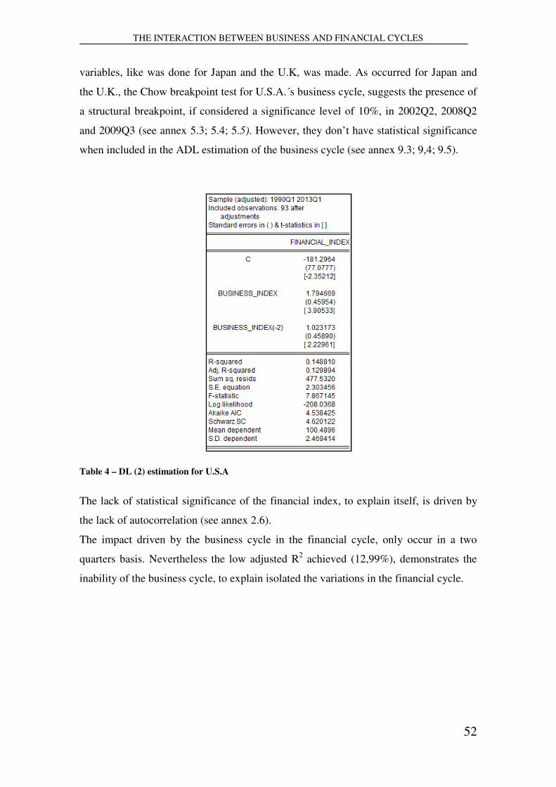
THE INTERACTION BETWEEN BUSINESS AND FINANCIAL CYCLES
52
variables, like was done for Japan and the U.K, was made. As occurred for Japan and
the U.K., the Chow breakpoint test for U.S.A.´s business cycle, suggests the presence of
a structural breakpoint, if considered a significance level of 10%, in 2002Q2, 2008Q2
and 2009Q3 (see annex 5.3; 5.4; 5.5). However, they don’t have statistical significance
when included in the ADL estimation of the business cycle (see annex 9.3; 9,4; 9.5).
Table 4 – DL (2) estimation for U.S.A
The lack of statistical significance of the financial index, to explain itself, is driven by
the lack of autocorrelation (see annex 2.6).
The impact driven by the business cycle in the financial cycle, only occur in a two
quarters basis. Nevertheless the low adjusted R2 achieved (12,99%), demonstrates the
inability of the business cycle, to explain isolated the variations in the financial cycle.
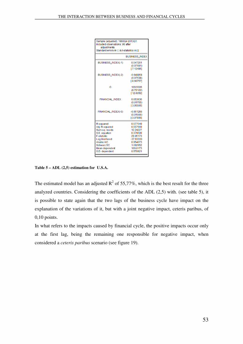
THE INTERACTION BETWEEN BUSINESS AND FINANCIAL CYCLES
53
Table 5 – ADL (2,5) estimation for U.S.A.
The estimated model has an adjusted R2 of 55,77%, which is the best result for the three
analyzed countries. Considering the coefficients of the ADL (2,5) with. (see table 5), it
is possible to state again that the two lags of the business cycle have impact on the
explanation of the variations of it, but with a joint negative impact, ceteris paribus, of
0,10 points.
In what refers to the impacts caused by financial cycle, the positive impacts occur only
at the first lag, being the remaining one responsible for negative impact, when
considered a ceteris paribus scenario (see figure 19).

THE INTERACTION BETWEEN BUSINESS AND FINANCIAL CYCLES
54
Figure 19 – The Business and Financial Index behavior of U.S.A., between the periods of 1989Q3-
2013Q1, quarterly data
From the analysis of the business cycle residuals (see Figure 20), it is possible to
disclose the volatility and the impact of other variables that weren’t considered in this
estimation. For instance, between the end of 2000 and the beginning of 2001, the U.S.A.
was not only suffering from the collapse of the “dot.com” bubble, as it was facing an
economic recession. The decrease of the GDP, due mainly to the increase of the
unemployment rate (the number of layoffs increased sharply, and companies start to
outsourcing their services), the fall in consumption levels and the raise of the inflation,
contributed to the increase of importance of exogenous factors in the business cycle,
which were not captured by the model.
Figure 20 - Business Index residuals of U.S.A., between the periods of 1989Q1-2013Q1, quarterly
data
From the analysis of the Dynamic Multipliers (see figure 21), it is possible conclude
that an impulse of one unit in the financial cycle cause a positive response in the
92
94
96
98
100
102
104
106
108
90 92 94 96 98 00 02 04 06 08 10 12
Business Index Financial Index

THE INTERACTION BETWEEN BUSINESS AND FINANCIAL CYCLES
55
business cycle during the moment 0, and the first period. However, it will induce
negative responses from the second period until the sixth period, where a readjustment
process begins, compensating the previous impacts. The negative impact in the fifth
period, after a brief “recovery” occurred in the fourth, is justified by the effect of the
inclusion the financial cycle fifth lag. Nevertheless, the fact that the business cycle
reacts negatively in the tenth period corroborates the presence of a cyclical behavior.
Figure 21 – Dynamic Multipliers for ADL (2,5) of U.S.A

THE INTERACTION BETWEEN BUSINESS AND FINANCIAL CYCLES
56
6.1.4 Aggregate view
From the individual analysis of each one of the three countries (Japan, U.K. and U.S.A),
and considering their importance in the global economy, there are some common
patterns from their business and financial cycles. The business cycle of Japan show
evidences of synchronization with the U.S.A´s business cycle, which is corroborated by
the similarity of their trends. However, the financial cycle of Japan does not have the
same behavior. It continues to show signals of underperformance, reflecting the impacts
felt in the financial system due to the “Japanese Asset Price Bubble”.
Regarding the fact that the three business cycles are all at the same stage (recovering
from a recession), the trend of the U.K´s business cycle is the one with fewer
similarities with the other countries. However, the business cycle trend in U.K is similar
to its own financial cycle. Nevertheless, it is important to verify that until the middle of
the 2001 year, the financial cycle trend of the U.K shows some common patterns with
the financial cycle of the U.S.A.. This can be justified by the economic zone where U.K.
is settled, and with its main trade partners.
The DL estimation for each country shows different results. In the case of Japan, the
impact of the business cycle in the financial cycle occurs contemporarily and with the
lag of one period. Nevertheless, for the U.S.A example the impact also occurs
contemporarily, but the lag with statistical significance is of two periods. The U.K. is a
particular case, where the past of the business cycle does not have statistical
significance to explain the present variations of the financial cycle.
According with the ADL model estimated for each country, in what concerns the impact
of the financial cycle in the business cycle, both Japan and U.S.A. show some common
features. In the U.K the negative impact of the financial cycle occurs at the first period,
when in the other two countries are at the fifth moment).
All the three countries under analysis expose the presence of structural break points in
the year of 2008, as consequence of the “Sub-prime” crisis in U.S.A., and the
“Sovereign Debt “crisis in Europe. However, when considered as a variable in the ADL
estimation, none of them have statistical significance.

THE INTERACTION BETWEEN BUSINESS AND FINANCIAL CYCLES
57
Chapter 7 – Conclusion Notes This dissertation aimed to evaluate the existence of relationships between business and
financial cycles in three of the most developed economies in the world.
Contrarily to what was expected, the business cycle, based in the data used in this study,
does not show statistical significance to explain the financial cycle.
As the result of the globalization process, when a severe financial disruption occurs, it
will spread its negative impacts in several economies worldwide, but with different
magnitude levels. The 2008 subprime crisis is a good example of this, starting in the
U.S.A, but ending up resulting in a sovereign debt crisis in Europe.
Regarding the existence of common patterns between the cycles of these countries, the
majority of the policies adopted to mitigate a crisis or to start recovery process of the
economy have some similarities. Each bubble burst, in a direct or indirect way, ends up
bringing negative impacts on the domestic economy. Governments spent millions of
dollars/yens/sterling pounds in order to stimulate the economy activity, injecting
liquidity in their financial systems, reforming their fiscal system, which in the majority
of the cases is insufficient to avoid the decrease of consumption levels and of the GDP.
However, it is important to notice that usually governments act too late, mainly after the
occurrence of a burst or recession, not demonstrating their policies to be pro-active
when the first signals of a bubble or a slow-down of the economy appear.
Despite the limitations imposed by the data collected and the indicators chosen, it was
possible to show that the financial cycles have influence in the movements of the
business cycle, and vice-versa, and an important role in the formation of peaks and
troughs.
Due to the natural cyclical behavior of the economy and the financial markets, taking in
account the result of a financial disruption have in the economy, and the long periods
for which their negative impacts remain valid in the economy, a more complete set of
surveillance measures should be implemented by the governments (e.g., like a set of
financial and macroeconomic indicators with control values determined by historical
reference standards observed in past bubbles and crisis)
For further investigation, it will be interesting to test the interactions between the
business and financial cycles with a larger data range, and with the inclusion of more
variables in the estimation model. This more complete picture can be able to seek in a

THE INTERACTION BETWEEN BUSINESS AND FINANCIAL CYCLES
58
more complete way an important question “Does the business cycle really influence the
financial cycle?”.
The study of these same relationships between economies with different stages of
development will be relevant to define a common standard trend in the business and
financial cycles all over the economic world.
Despite the efforts of supervisors to create and to impose rules in the financial system,
the increasing complexity of the financial instruments continuous to maintain a gap,
those investors will try to explore, which will spread its effects on the business cycle.
By this way, maybe it is more important to first understand the dynamics and chain of
events betweens those cycles, and then adapt the regulation in order to increase its
efficiency.
For further investigation, will be interesting testing the interactions between the
business and financial cycles with a larger set of data, and with the inclusion of more
indicators in the estimation model. This more complete approach, will seek essentially
respond to the question “Does the business cycle really influence the financial cycle?”.
Also, studying these same relationships between economies with different stages of
development, will be relevant, in order to define a common standard trend in the
business and financial cycles all over the world.
Due to the continuously deregulation of the financial system, it will be important
understand, how this fact is affecting the behavior of the financial cycle, allowing to
understand if the deregulation of the markets, are increasing the impacts of the financial
cycle in the economies.
THE INTERACTION BETWEEN BUSINESS AND FINANCIAL CYCLES
59
References Baltagi, B. 2011. Econometrics (5th ed.). Berlin: Springer. Bodie, Z., Kane, A., & Marcus, A. J. 2009. Investments (8th ed.). New York: McGraw-Hill Irwin.
Box, G. E. P., & Pierce, D. A. 1970. Distribution of Residual Correlations in Autoregressive-integrated Moving Average Time Series Models. Journal of the
American Statistical Association, 65: 1509–1526. Buiter, W. H,, Corsetti, G. M., & Pesenti, P. A. 1998. Interpreting the ERM Crisis: Coutry-specific and Systemic issues. Princeton Studies in International Finance, 88. New Jersey: Princeton University Burns, A., & Mitchell, W. 1946. Measuring business cycles. New York: National Bureau of Economic Research, Inc Case, B., Goetzmann, W., N., & Rouwenhorst, K., G. 2000. Global Real Estate Markets - Cycles and Fundamentals. National Bureau of Economic Research, Working Paper 7566. Case, K., Quigley, J., Shiller, R. 2003. Home-buyers, Housing and the
Macroeconomy. Paper presented at the Reserve Bank of Australia Conference on Asset Prices and Monetary Policy (August). Chauvet, M., & Potter, S. 2000. Coincident and leading indicators of the stock market. Journal of Empirical Finance, 7(1): 87-111. Claessens, S., Kose, M. A., & Terrones, M. E., 2011a. How Do Business and Financial Cycles Interact?. International Monetary Fund, Working Papers 11/88. Claessens, S., Kose, M. A., & Terrones, M. E., 2011b. Financial Cycles: What? How? When?. International Monetary Fund, Working Papers 11/76. Diebolt, C., & Doliger, C. 2008. New International Evidence on the Cyclical Behaviour of Output: Kuznets Swings Reconsidered. Quality & Quantity: International Journal
of Methodology, 42(6): 719–737. Dickey, D.,& Fuller, W. 1979.Distribution of the estimators for Autoregressive Time Series with a Unit Root. Journal of the American Statistical Association, 74: 427-431. Ducos, G. 1997. Clément Juglar. In Glasner, D.(ed), Business Cycles and Depressions.
An Encyclopedia: 345-347. New York and London: Garland Publishing Inc.. Economic Planning Agency of Japan. 1994. Economic Survey of Japan (1993-1994):
A Challenge to New Frontiers Beyond the Severe Adjustment Process. Tokyo: EPA.

THE INTERACTION BETWEEN BUSINESS AND FINANCIAL CYCLES
60
Edwards, S., & Biscarri, J. G., & Perez de Gracia, F. 2003. Stock market cycles, financial liberalization and volatility. Journal of International Money and Finance, 22(7): 925-955. Fama, E., F. 1965. The Behavior of Stock-Market Prices. The Journal of Business, 38(1): 34-105. Flath, D. 2000. The Japanese Economy (1st ed.). Oxford: Oxford University Press Galbraith, J. K. 1954. The Great Crash 1929.Boston: Houghton, Mifflin Company.
Hamilton, J. 1994. Time Series Analysis. New Jersey: Princeton University Press.
Herring, R., & Wachter, S. 1999. Real Estate Booms and Banking Busts-An International Perspective. Group of Thirty, occasional paper 58.
Hott, C., 2009. Banks and Real Estate Prices. The Swiss National Bank, Working Paper 2009-8.
Jarque, C. and Bera, 1980.Efficient Test for Normality, Homoscedasticity and serial independence of regressions residuals. Economics Letters, 6 (3): 225-259.
Jenkins, J. 2010. The Labour Market in the 1980s, 1990s and 2008/09 Recessions. Economic & Labour Market Review, 4 (8): 29-36.
Juglar, C. 1862.Des Crises commerciales et de leur retour periodique en France, en
Angleterre, et aux Etats-Unis. Paris: Libraire Gillaumin. et Cie.
Kaiser, R., W., 1997. The Long Cycle of Real Estate. Journal of Real Estate Research, 14(3): 233-258.
Kindleberger, C. P., & Aliber, R. Z. 2005. Manias, Panics and Crashes: A History of
Financial Crises (5th ed.) .London: Palgrave Macmillan. Kitchin, J. 1923. Cycles and Trends in Economic Factor. Review of Economic and
Statistics, 5 (1): 10-16. Kiyotaki, N., & Moore, J. 1995. Credit Cycles. National Bureau of Economic
Research, Working Paper 5083. Kondratieff, N.D. 1926 [1979]. The Long Waves in Economic Life. Review, 2(4):519-562. Kuznets, S. 1930. Secular Movements in Production and Prices. Their Nature and
their Bearing upon Cyclical Fluctuations. Boston: Houghton Mifflin. Kwiatkowski D., P. Phillips, Schmidt, P.,& Shin, Y. 1992.Testing the Null Hypothesis of Stationarity against the Alternative of a Unit Root. Journal of Econometrics, 54: 159-178.

THE INTERACTION BETWEEN BUSINESS AND FINANCIAL CYCLES
61
Lambertini, L. Mendicino, C., & Punzi, M., T. 2011. Leaning Against Boom-Bust Cycles in Credit and Housing Prices. Banco de Portugal, Working Paper 8/11. Leigh, A., Wolfers, J., & Zitzewitz, E. 2003. What do Financial Markets think of War in Iraq?. National Bureau of Economic Research, Working Paper 9587. Liew, V. 2004. Which Lag Length Selection Criteria Should We Employ? Economics
Bulletin, 33(33): 1-9. Minsky, H. P.1992. The Financial Instability Hypothesis. Economics Working Paper
Archive. 74. OECD. 2004. OECD Economic Surveys of United Kingdom 2004. Paris OECD. 2009.OECD Economic Surveys of United Kingdom 2009. Paris OECD. 2010. OECD Economic Surveys of United States 2010. Paris OECD. 2011a. OECD Economic Surveys of Japan 2011. Paris OECD. 2011b. OECD Economic Surveys of United Kingdom 2011. Paris OECD. 2012. OECD Economic Surveys of United States 2012. Paris OECD. 2013a. OECD Economic Surveys of Japan 2013. Paris OECD. 2013b. OECD Economic Surveys of United Kingdom 2013. Paris. Pagan, A. R. & Sossounov, K. A., 2003. A simple framework for analyzing bull and bear markets. Journal of Applied Econometrics, 18(1): 23-46. Papageorgiou, A., & Tsoulfidis, L. 2006. Kondratiev, Marx and the Long cycle. Indian Development Review. In Mariolis, T.,& Tsoulfidis, L. (Eds.), Distribution,
development and prices, critical perspectives. New Delhi: Serials Phillips, P., & Perron, P. 1988. Testing for a Unit Root in Time Series Regression. Biometrika,75: 335-346. Poterba, J. M. 1991. House Price Dynamics: The Role of Tax Policy and Demography. Brookings Papers on Economic Activity, 2: 143-183. Schumpeter, J.A. 1934. The Theory of Economic Development. Cambridge, Massachusetts: Harvard University Press. Schumpeter, J.A. 1939. Business Cycles: A Theoretical, Historical, and Statistical
Analysis of the Capitalist Process. New York and London: McGraw-Hill. Schumpeter, J. 1954. History of economic analysis. London: Allen and Unwin.

THE INTERACTION BETWEEN BUSINESS AND FINANCIAL CYCLES
62
Shiller, R., 2005.Irrational Exuberance (2nd ed.). New Jersey: Princeton University Press. Shiller, R. 2007. "Understanding Recent Trends in House Prices and Home Ownership". National Bureau of Economic Research, Working Paper 13553. Silva, R. 2012.The Investor Behavior on Extreme Situations of Speculation and Crash: An approach based on Iterated Prisoner´s Dilemma. International Journal of the latest
trends in Finance and Economic Science, 2 (3): 169-189. Sismondi, J. C. L. 1819 [1991]. New Principles of Political Economy of Wealth in its
Relation to Population. New Brunswick: Transaction Publishers. Syed, M., Kang, K., & Tokuoka, K. 2009. “Lost Decade” in Translation: What Japan´s Crisis could Portbend about Recovery from the Great Recession. International
Monetary Fund, Working Paper WP/09/282.
White, E. N. 1990. The Stock Market Boom and Crash of 1929 Revisited. The Journal
of Economic Perspectives, 4 (2): 67-83.
Other References Bloomberg Hardware
FRED
http://research.stlouisfed.org/fred2/series/GBRRECDM http://research.stlouisfed.org/fred2/series/JPNRECP ITA
http://tse.export.gov/TSE/MapDisplay.aspx
NBER
http://www.nber.org/cycles.html
OECD
http://stats.oecd.org/Index.aspx?DataSetCode=MEI_CLI http://stats.oecd.org/viewhtml.aspx?datasetcode=MEI_PRICES&lang=en#
Thomson Reuters Datastream
http://online.thomsonreuters.com/datastream/

THE INTERACTION BETWEEN BUSINESS AND FINANCIAL CYCLES
63
Annex 1- Correlations Annex 1.1 – Correlation between Business and Financial Indexes, Japan
Annex 1.2 - Correlation between Business and Financial Indexes, U.K.
Annex 1.3 - Correlation between Business and Financial Indexes, U.S.A.

THE INTERACTION BETWEEN BUSINESS AND FINANCIAL CYCLES
64
Annex 2 - Autocorrelations
Annex 2.1 – Autocorrelation Business Index, Japan

THE INTERACTION BETWEEN BUSINESS AND FINANCIAL CYCLES
65
Annex 2.2 – Autocorrelation Financial Index, Japan

THE INTERACTION BETWEEN BUSINESS AND FINANCIAL CYCLES
66
Annex 2.3 – Autocorrelation Business Index, U.K.

THE INTERACTION BETWEEN BUSINESS AND FINANCIAL CYCLES
67
Annex 2.4 – Autocorrelation Financial Index, U.K.

THE INTERACTION BETWEEN BUSINESS AND FINANCIAL CYCLES
68
Annex 2.5 – Autocorrelation Business Index, U.S.A.

THE INTERACTION BETWEEN BUSINESS AND FINANCIAL CYCLES
69
Annex 2.6 – Autocorrelation Financial Index, U.S.A.

THE INTERACTION BETWEEN BUSINESS AND FINANCIAL CYCLES
70
Annex 3 – Normality Tests
Annex 3.1 – ADL Residual Normality Test between Business and Financial Index, Japan
Annex 3.2 – ADL Residual Normality Test between Business and Financial Index, U.K.
Annex 3.3 – ADL Residual Normality Test between Business and Financial Index, U.S.A.

THE INTERACTION BETWEEN BUSINESS AND FINANCIAL CYCLES
71
Annex 4 – Unit Root Tests
Annex 4.1 - Unit Root test to Business_Index using ADF, to Japan
Annex 4.2 - Unit Root test to Financial_Index using ADF, to Japan
Annex 4.3 - Unit Root test to Business_Index using PP, to Japan

THE INTERACTION BETWEEN BUSINESS AND FINANCIAL CYCLES
72
Annex 4.4 - Unit Root test to Financial_Index using PP, to Japan
Annex 4.5 - Unit Root test to Business_Index using KPSS, to Japan
Annex 4.6 - Unit Root test to Financial_Index using KPSS, to Japan

THE INTERACTION BETWEEN BUSINESS AND FINANCIAL CYCLES
73
Annex 4.7 - Unit Root test to Business_Index using ADF, to U.K.
Annex 4.8 - Unit Root test to Financial_Index using ADF, to U.K.
Annex 4.9 - Unit Root test to Business_Index using PP, to U.K.

THE INTERACTION BETWEEN BUSINESS AND FINANCIAL CYCLES
74
Annex 4.10 - Unit Root test to Financial_Index using PP, to U.K.
Annex 4.11 - Unit Root test to Business_Index using KPSS, to U.K.
Annex 4.12 - Unit Root test to Financial_Index using KPSS, to U.K.

THE INTERACTION BETWEEN BUSINESS AND FINANCIAL CYCLES
75
Annex 4.13 - Unit Root test to Business_Index using ADF, to U.S.A.
Annex 4.14 - Unit Root test to Financial_Index using ADF, to U.S.A.
Annex 4.15 - Unit Root test to Business_Index using PP, to U.S.A.

THE INTERACTION BETWEEN BUSINESS AND FINANCIAL CYCLES
76
Annex 4.16- Unit Root test to Financial_Index using PP, to U.S.A.
Annex 4.17 - Unit Root test to Business_Index using KPSS, to U.S.A.
Annex 4.18 - Unit Root test to Financial_Index using KPSS, to U.S.A.

THE INTERACTION BETWEEN BUSINESS AND FINANCIAL CYCLES
77
Annex 5 – Chow Breakpoint Tests
Annex 5.1 – Chow Breakpoint Test, Japan (2008Q2)
Annex 5.2 –Chow Breakpoint Test, U.K. (2008Q4)
Annex 5.3 –Chow Breakpoint Test, U.S.A. (2002Q2)
Annex 5.4 –Chow Breakpoint Test, U.S.A. (2008Q2)

THE INTERACTION BETWEEN BUSINESS AND FINANCIAL CYCLES
78
Annex 5.5 –Chow Breakpoint Test, U.S.A. (2009Q3)

THE INTERACTION BETWEEN BUSINESS AND FINANCIAL CYCLES
79
Annex 6 – Granger Causality Test
Annex 6.1 - Granger Causality test for Japan.
Annex 6.2 - Granger Causality test for U.K.
Annex 6.3 - Granger Causality test for U.S.A.
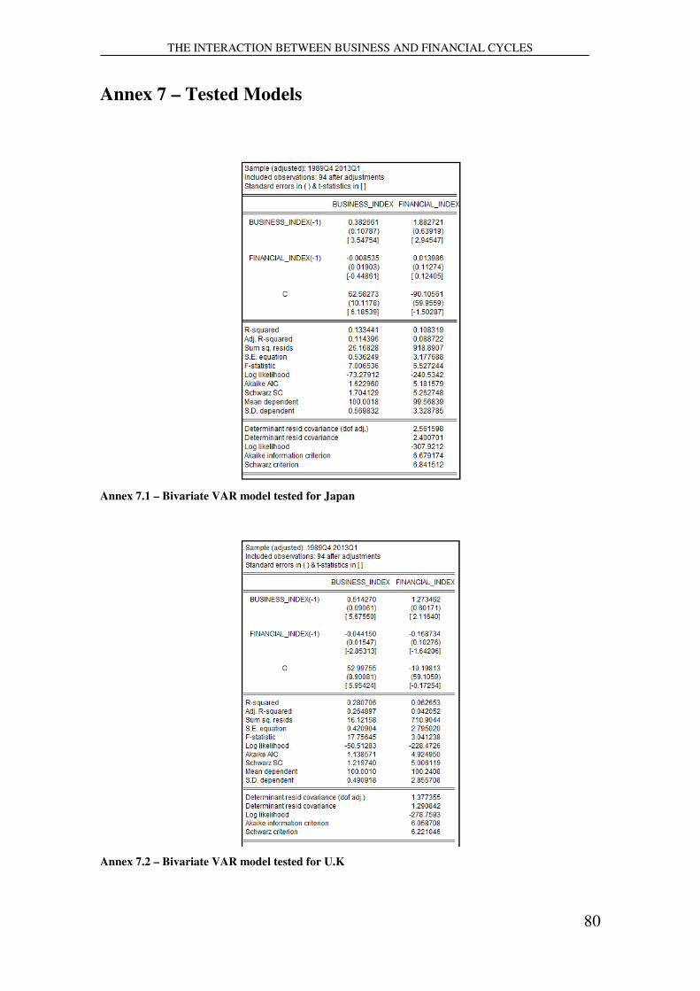
THE INTERACTION BETWEEN BUSINESS AND FINANCIAL CYCLES
80
Annex 7 – Tested Models
Annex 7.1 – Bivariate VAR model tested for Japan
Annex 7.2 – Bivariate VAR model tested for U.K

THE INTERACTION BETWEEN BUSINESS AND FINANCIAL CYCLES
81
Annex 7.3 – Bivariate VAR model tested for U.S.A.

THE INTERACTION BETWEEN BUSINESS AND FINANCIAL CYCLES
82
Annex 8 – Lag Order Selection
Annex 8.1 – ADL Lag Order Selection Criteria of Japan

THE INTERACTION BETWEEN BUSINESS AND FINANCIAL CYCLES
83
Annex 8.2 – ADL Log Order Selection Criteria of U.K.

THE INTERACTION BETWEEN BUSINESS AND FINANCIAL CYCLES
84
Annex 8.3 – ADL Log Order Selection Criteria of U.S.A.

THE INTERACTION BETWEEN BUSINESS AND FINANCIAL CYCLES
85
Annex 9 – Models with Dummies
Annex 9.1 - ADL (2,5) with dummy 2008Q2 estimation of Japan

THE INTERACTION BETWEEN BUSINESS AND FINANCIAL CYCLES
86
Annex 9.2 - ADL (2,1) with dummy 2008Q2 estimation of U.K.

THE INTERACTION BETWEEN BUSINESS AND FINANCIAL CYCLES
87
Annex 9.3 - ADL (2,5) with dummy 2002Q2 estimation of U.S.A

THE INTERACTION BETWEEN BUSINESS AND FINANCIAL CYCLES
88
Annex 9.4 - ADL (2,5) with dummy 2008Q2 estimation of U.S.A

THE INTERACTION BETWEEN BUSINESS AND FINANCIAL CYCLES
89
Annex 9.5 - ADL (2,5) with dummy 2009Q3 estimation of U.S.A