Embed Size (px)
Citation preview

Chapter 4

THE INTENSITY-DEPENDENT REFRACTIVE INDEX
▪ 4.1. Descriptions of the Intensity-Dependent Refractive Index
▪ 4.2. Tensor Nature of the Third-Order Susceptibility
▪ 4.3. Nonresonant Electronic Nonlinearities
▪ 4.4. Nonlinearities Due to Molecular Orientation
▪ 4.5. Thermal Nonlinear Optical Effects
▪ 4.6. Semiconductor Nonlinearities
▪ 4.7. Concluding Remarks
2
4.1. Descriptions of the Intensity-Dependent Refractive Index
where n0 represents the usual, weak-field refractive index and തn2 is sometimes called the
second-order index of refraction.
The angular brackets surrounding the quantity ෩E2 represent a time average. Thus, if the
optical field is of the form
The refractive index of many materials can be described by the relation
3
The change in refractive index described by Eq. (4.1.1) or (4.1.4) is sometimes called the
optical Kerr effect.
The refractive index of a material changes by an amount that is proportional to the square
of the strength of an applied static electric field.
The part of the nonlinear polarization that influences the propagation of a beam of frequency ω
is
4
5
where we have introduced the effective susceptibility
and by introducing Eq. (4.1.4) on the left-hand side and Eq. (4.1.7) on the right-hand side of this equation, we
find that
6
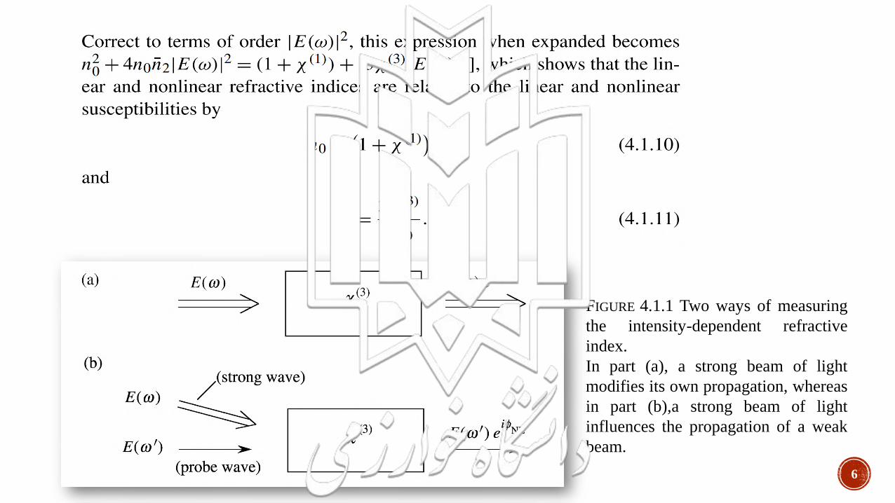
FIGURE 4.1.1 Two ways of measuring
the intensity-dependent refractive
index.
In part (a), a strong beam of light
modifies its own propagation, whereas
in part (b),a strong beam of light
influences the propagation of a weak
beam.
7
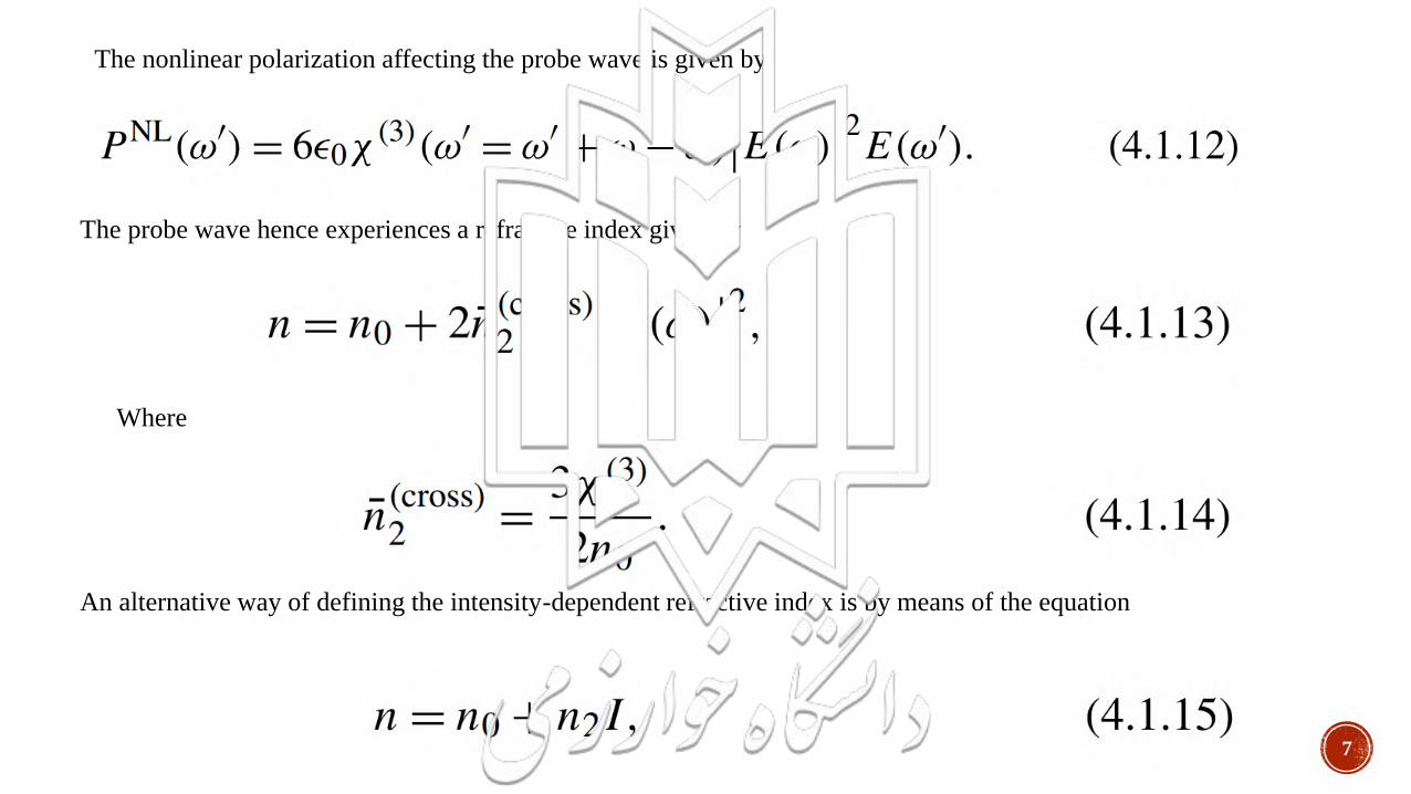
The nonlinear polarization affecting the probe wave is given by
The probe wave hence experiences a refractive index given by
Where
An alternative way of defining the intensity-dependent refractive index is by means of the equation
8
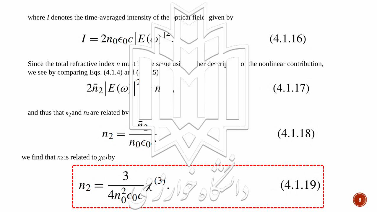
where I denotes the time-averaged intensity of the optical field, given by
Since the total refractive index n must be the same using either description of the nonlinear contribution,
we see by comparing Eqs. (4.1.4) and (4.1.15) that
and thus that n2and n2 are related by
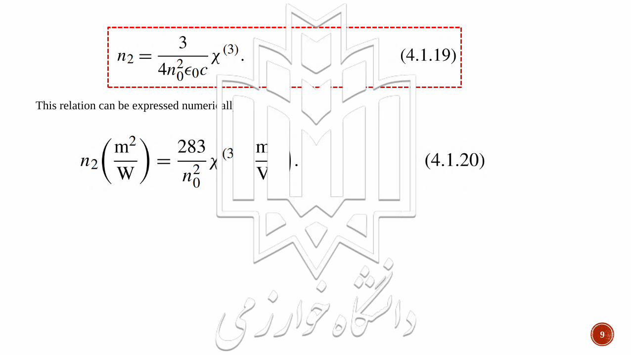
we find that n2 is related to χ(3) by
9
This relation can be expressed numerically as
10
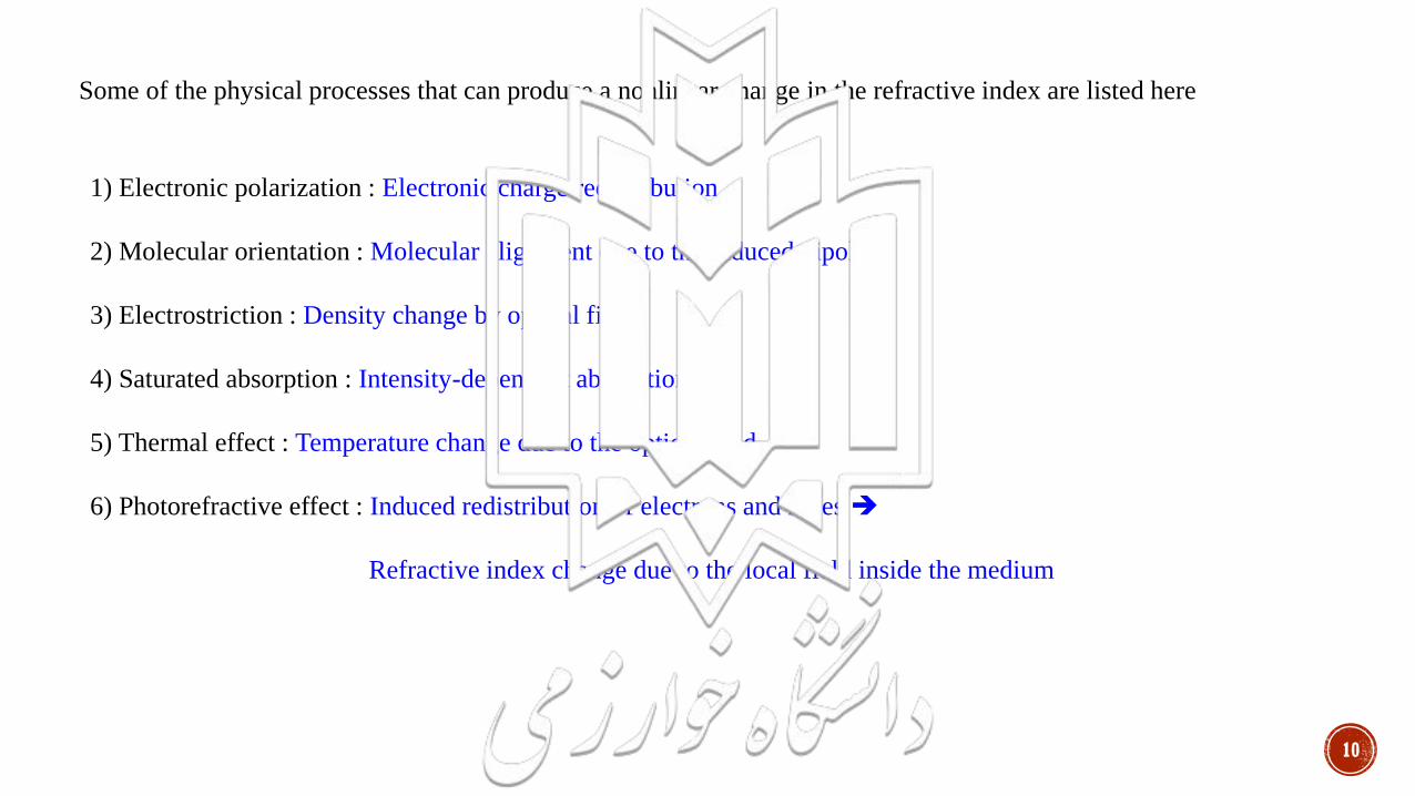
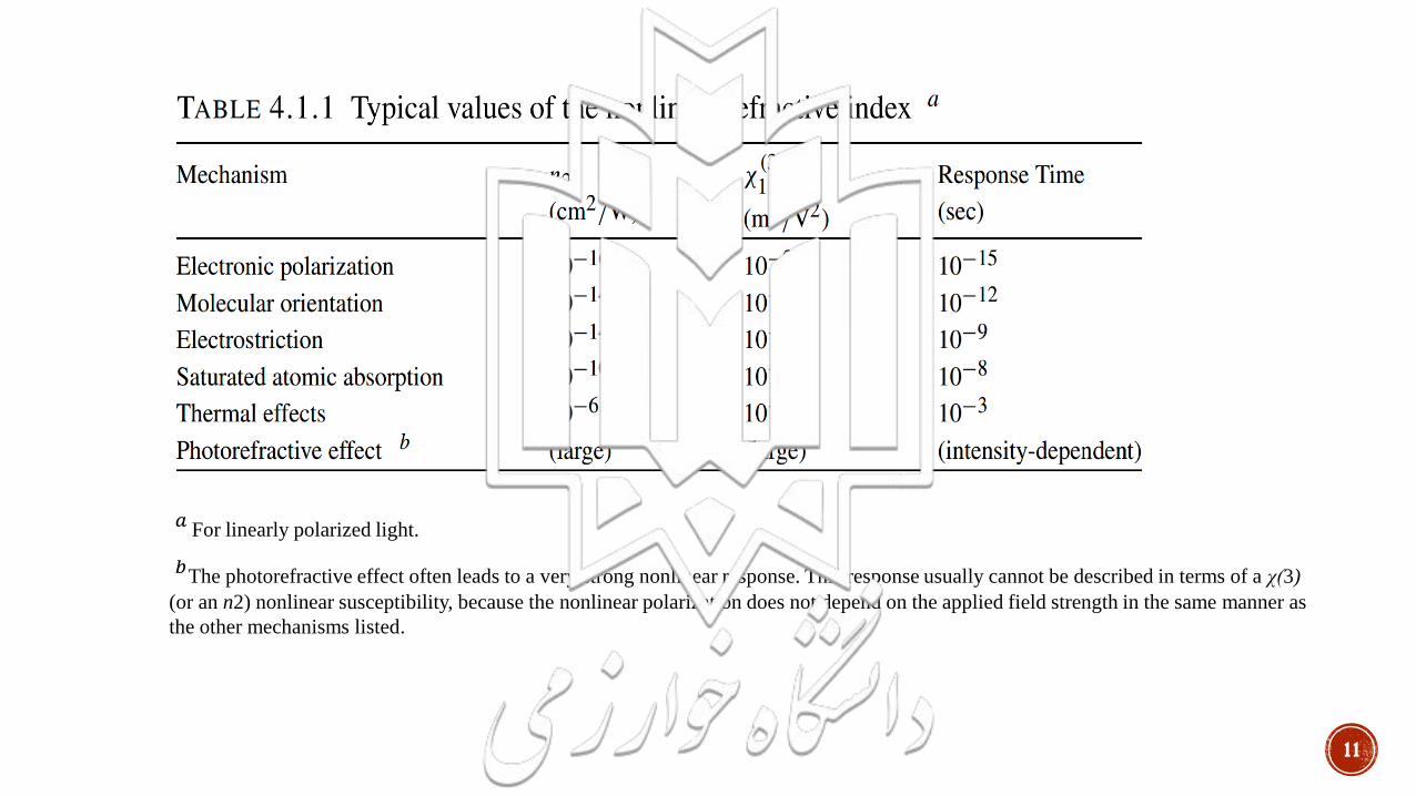
Some of the physical processes that can produce a nonlinear change in the refractive index are listed here
1) Electronic polarization : Electronic charge redistribution
2) Molecular orientation : Molecular alignment due to the induced dipole
3) Electrostriction : Density change by optical field
4) Saturated absorption : Intensity-dependent absorption
5) Thermal effect : Temperature change due to the optical field
6) Photorefractive effect : Induced redistribution of electrons and holes ➔
Refractive index change due to the local field inside the medium
11
𝑎For linearly polarized light.
𝑏The photorefractive effect often leads to a very strong nonlinear response. This response usually cannot be described in terms of a χ(3)
(or an n2) nonlinear susceptibility, because the nonlinear polarization does not depend on the applied field strength in the same manner as
the other mechanisms listed.

THE INTENSITY-DEPENDENT REFRACTIVE INDEX
▪ 4.1. Descriptions of the Intensity-Dependent Refractive Index
▪ 4.2. Tensor Nature of the Third-Order Susceptibility
▪ 4.3. Nonresonant Electronic Nonlinearities
▪ 4.4. Nonlinearities Due to Molecular Orientation
▪ 4.5. Thermal Nonlinear Optical Effects
▪ 4.6. Semiconductor Nonlinearities
▪ 4.7. Concluding Remarks
12
13
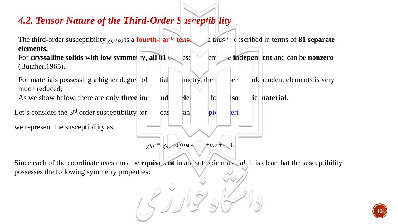
4.2. Tensor Nature of the Third-Order Susceptibility
The third-order susceptibility χijkl (3) is a fourth-rank tensor, and thus is described in terms of 81 separate
elements.
For crystalline solids with low symmetry, all 81 of these elements are independent and can be nonzero
(Butcher,1965).
For materials possessing a higher degree of spatial symmetry, the number of independent elements is very
much reduced;
As we show below, there are only three independent elements for an isotropic material.
we represent the susceptibility as
χijkl ≡ χijkl (3) (ω4 = ω1 +ω2 +ω3).
Since each of the coordinate axes must be equivalent in an isotropic material, it is clear that the susceptibility
possesses the following symmetry properties:
Let’s consider the 3rd order susceptibility for the case of an isotropic material.
14
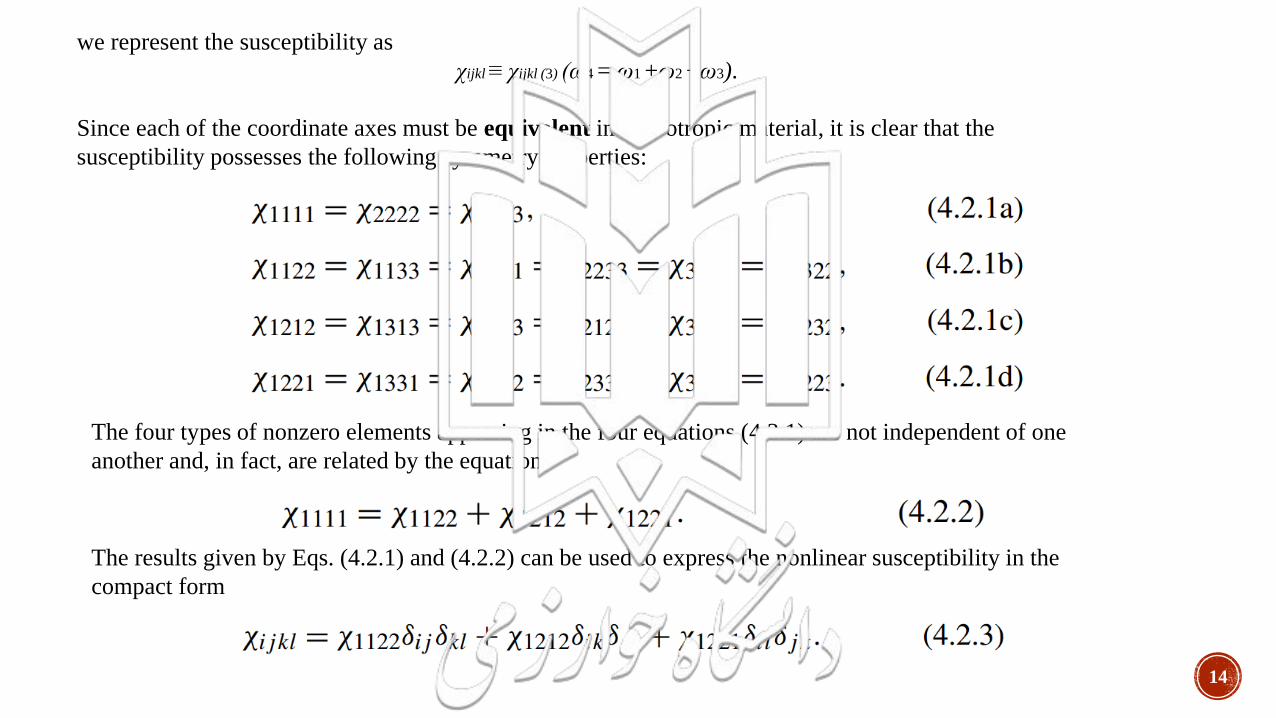
we represent the susceptibility as
χijkl ≡ χijkl (3) (ω4 = ω1 +ω2 +ω3).
Since each of the coordinate axes must be equivalent in an isotropic material, it is clear that the
susceptibility possesses the following symmetry properties:
The four types of nonzero elements appearing in the four equations (4.2.1) are not independent of one
another and, in fact, are related by the equation
The results given by Eqs. (4.2.1) and (4.2.2) can be used to express the nonlinear susceptibility in the
compact form
15
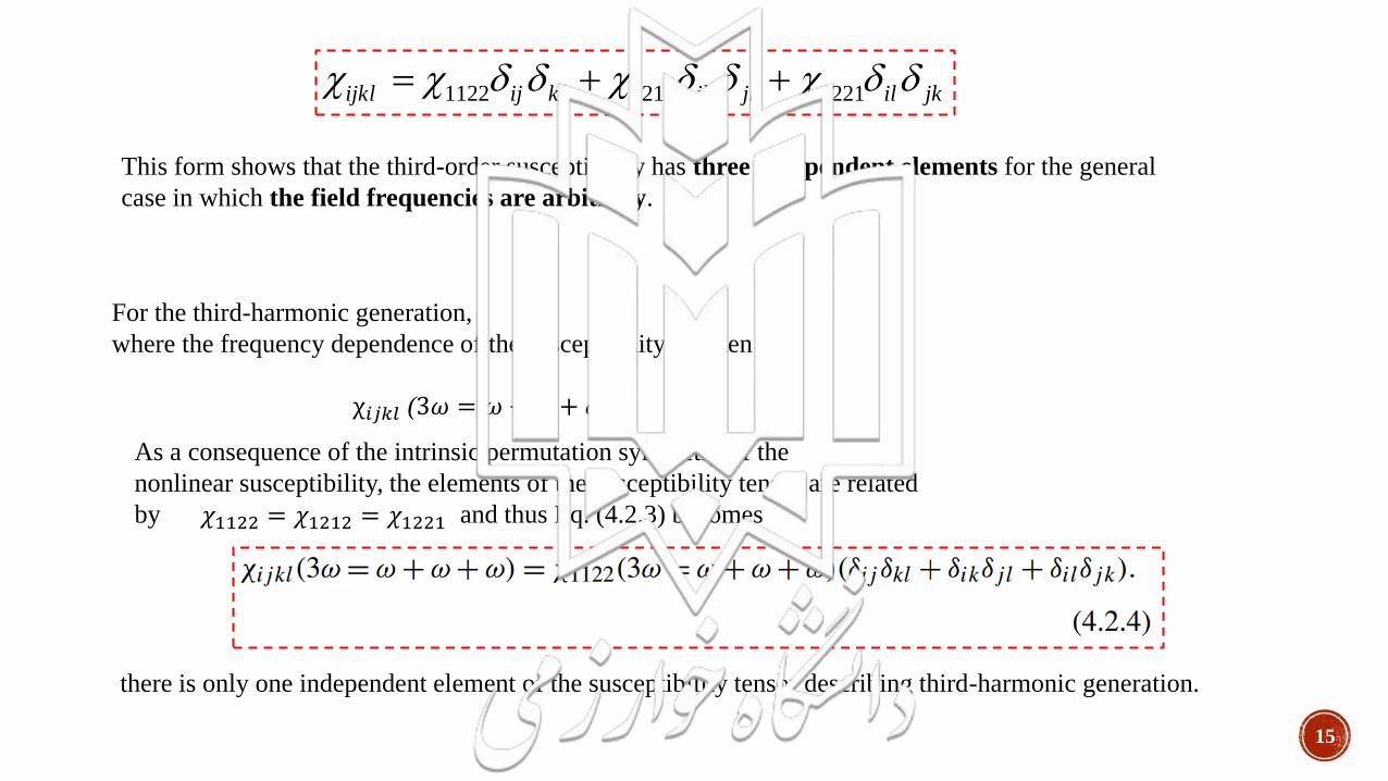
1122 1212 1221ijkl ij kl ik jl il jk = + +
This form shows that the third-order susceptibility has three independent elements for the general
case in which the field frequencies are arbitrary.
For the third-harmonic generation,
where the frequency dependence of the susceptibility is taken as
χ𝑖𝑗𝑘𝑙 (3𝜔 = 𝜔 + 𝜔 + 𝜔)
As a consequence of the intrinsic permutation symmetry of the
nonlinear susceptibility, the elements of the susceptibility tensor are related
by and thus Eq. (4.2.3) becomes𝜒1122 = 𝜒1212 = 𝜒1221
there is only one independent element of the susceptibility tensor describing third-harmonic generation.
16
Now, we consider the choice of frequencies given
χ𝑖𝑗𝑘𝑙 (3𝜔 = 𝜔 + 𝜔 − 𝜔)
For this choice of frequencies, the condition of intrinsic permutation symmetry requires that
χ1122 be equal to χ1212, and hence χ𝑖𝑗𝑘𝑙 can be represented by
The nonlinear polarization leading to the nonlinear refractive index is given in terms of the nonlinear
susceptibility by
If we introduce Eq. (4.2.5) into this equation, we find that
17
This equation can be written entirely in vector form as
Following the notation of Maker and Terhune (1965) (see also Maker et al., 1964), we introduce the
coefficients
in terms of which the nonlinear polarization of Eq. (4.2.8) can be written as
18
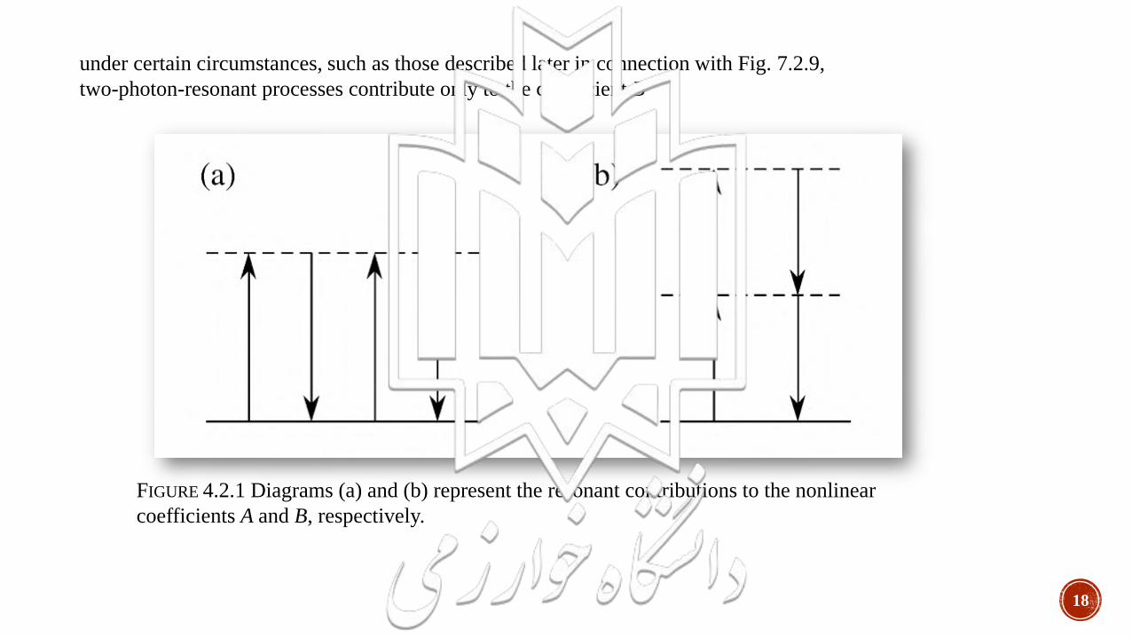
under certain circumstances, such as those described later in connection with Fig. 7.2.9,
two-photon-resonant processes contribute only to the coefficient B
FIGURE 4.2.1 Diagrams (a) and (b) represent the resonant contributions to the nonlinear
coefficients A and B, respectively.
19
For some purposes, it is useful to describe the nonlinear polarization not by Eq. (4.2.10) but rather in terms of
an effective linear susceptibility defined by means of the relationship
Then, as can be verified by direct substitution, Eqs. (4.2.10) and (4.2.11) lead to identical predictions for the
nonlinear polarization if the effective linear susceptibility is given by
20
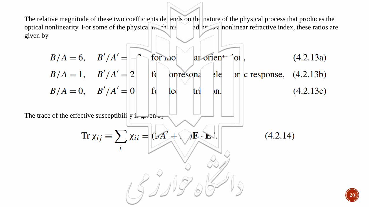
The relative magnitude of these two coefficients depends on the nature of the physical process that produces the
optical nonlinearity. For some of the physical mechanisms leading to a nonlinear refractive index, these ratios are
given by
The trace of the effective susceptibility is given by
21
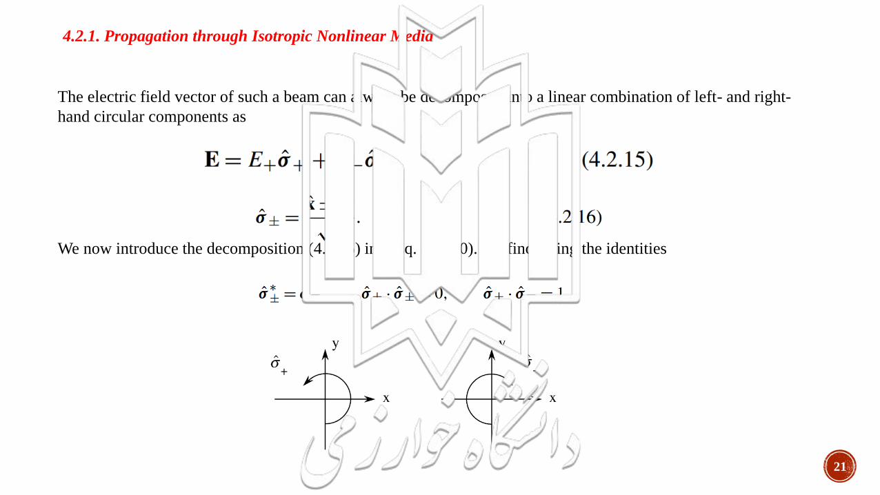
4.2.1. Propagation through Isotropic Nonlinear Media
The electric field vector of such a beam can always be decomposed into a linear combination of left- and right-
hand circular components as
We now introduce the decomposition (4.2.15) into Eq. (4.2.10). We find, using the identities
22
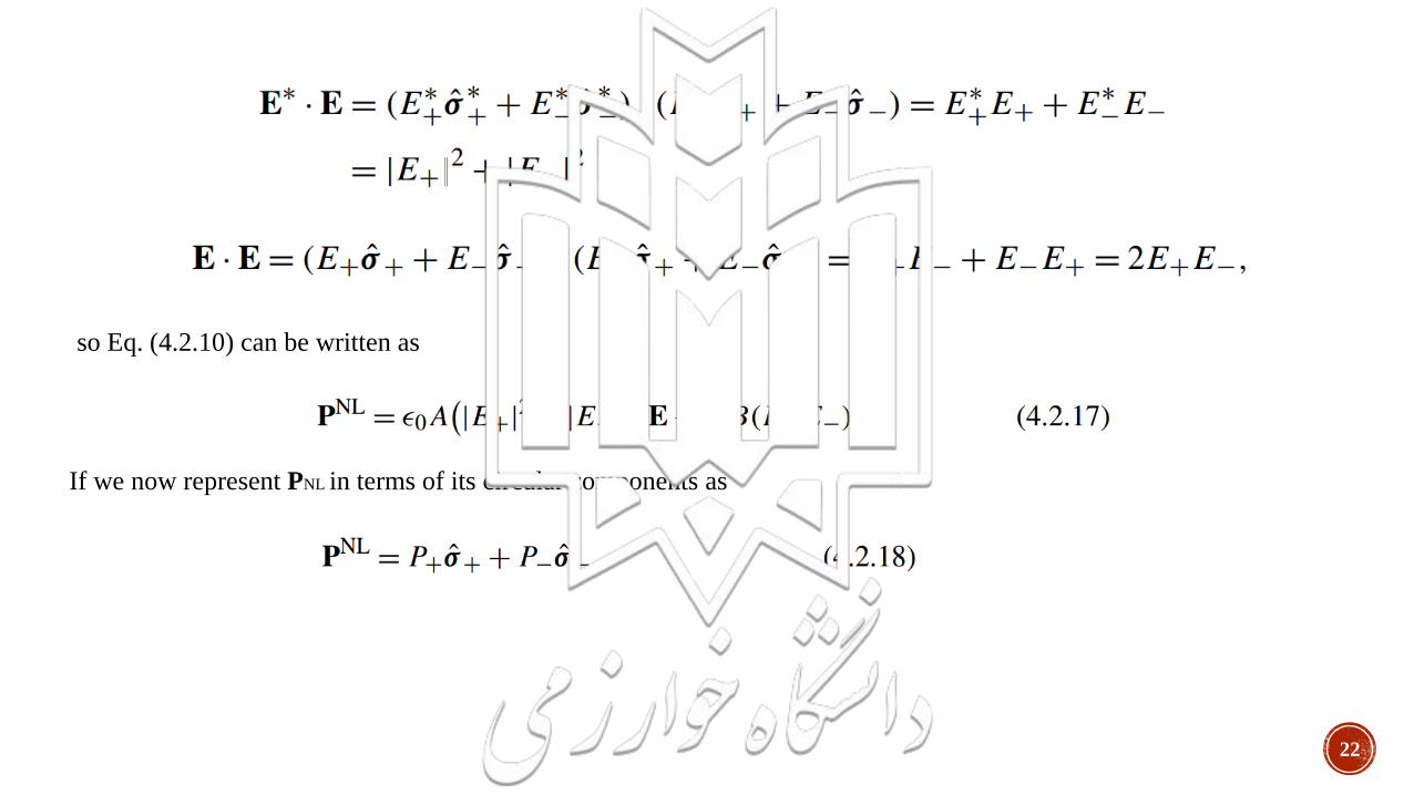
so Eq. (4.2.10) can be written as
If we now represent PNL in terms of its circular components as
23
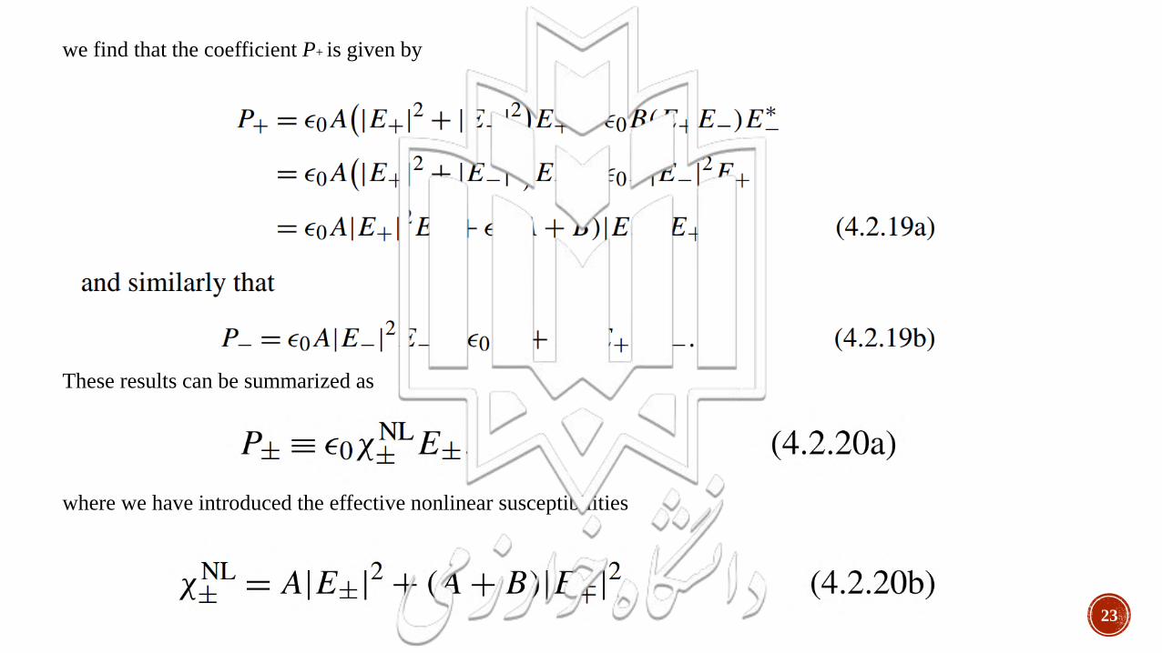
we find that the coefficient P+ is given by
These results can be summarized as
where we have introduced the effective nonlinear susceptibilities
24
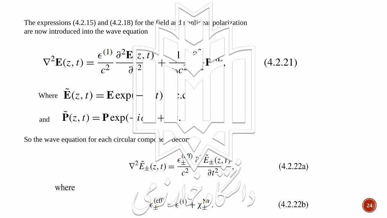
The expressions (4.2.15) and (4.2.18) for the field and nonlinear polarization
are now introduced into the wave equation
Where
and
So the wave equation for each circular component becomes
25
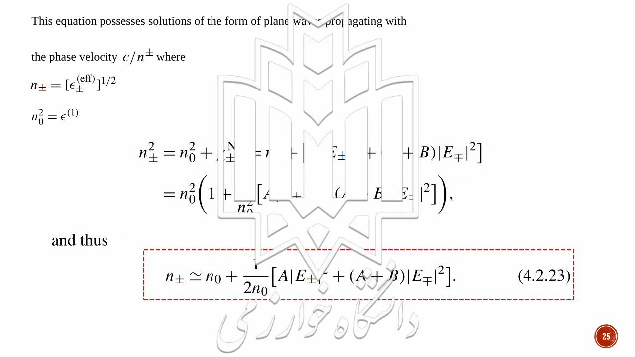
This equation possesses solutions of the form of plane waves propagating with
the phase velocity where
26
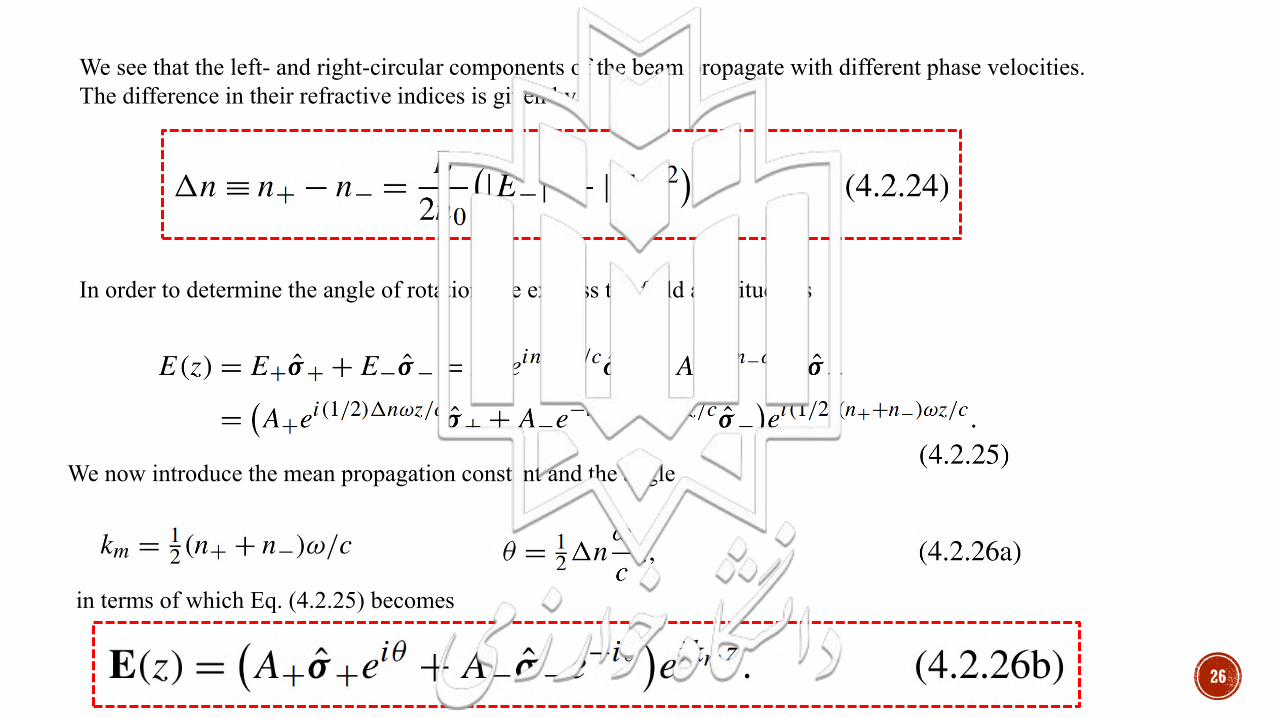
We see that the left- and right-circular components of the beam propagate with different phase velocities.
The difference in their refractive indices is given by
In order to determine the angle of rotation, we express the field amplitude as
We now introduce the mean propagation constant and the angle
in terms of which Eq. (4.2.25) becomes
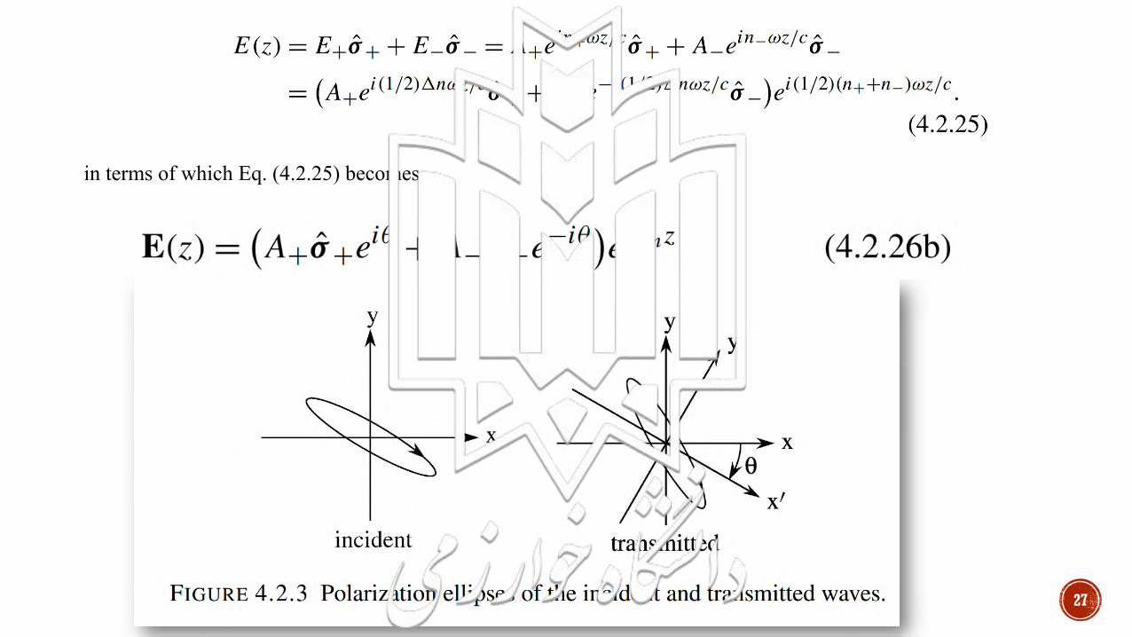
27
in terms of which Eq. (4.2.25) becomes
28
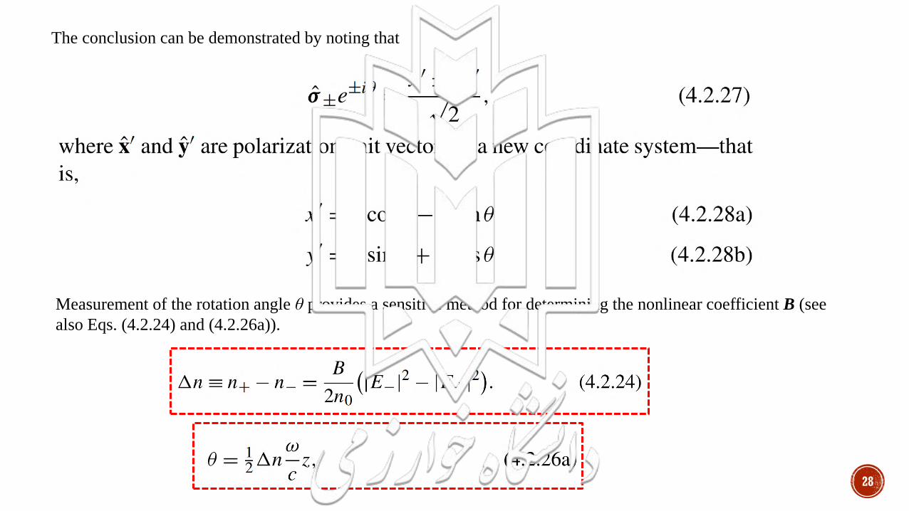
The conclusion can be demonstrated by noting that
Measurement of the rotation angle θ provides a sensitive method for determining the nonlinear coefficient B (see
also Eqs. (4.2.24) and (4.2.26a)).
29
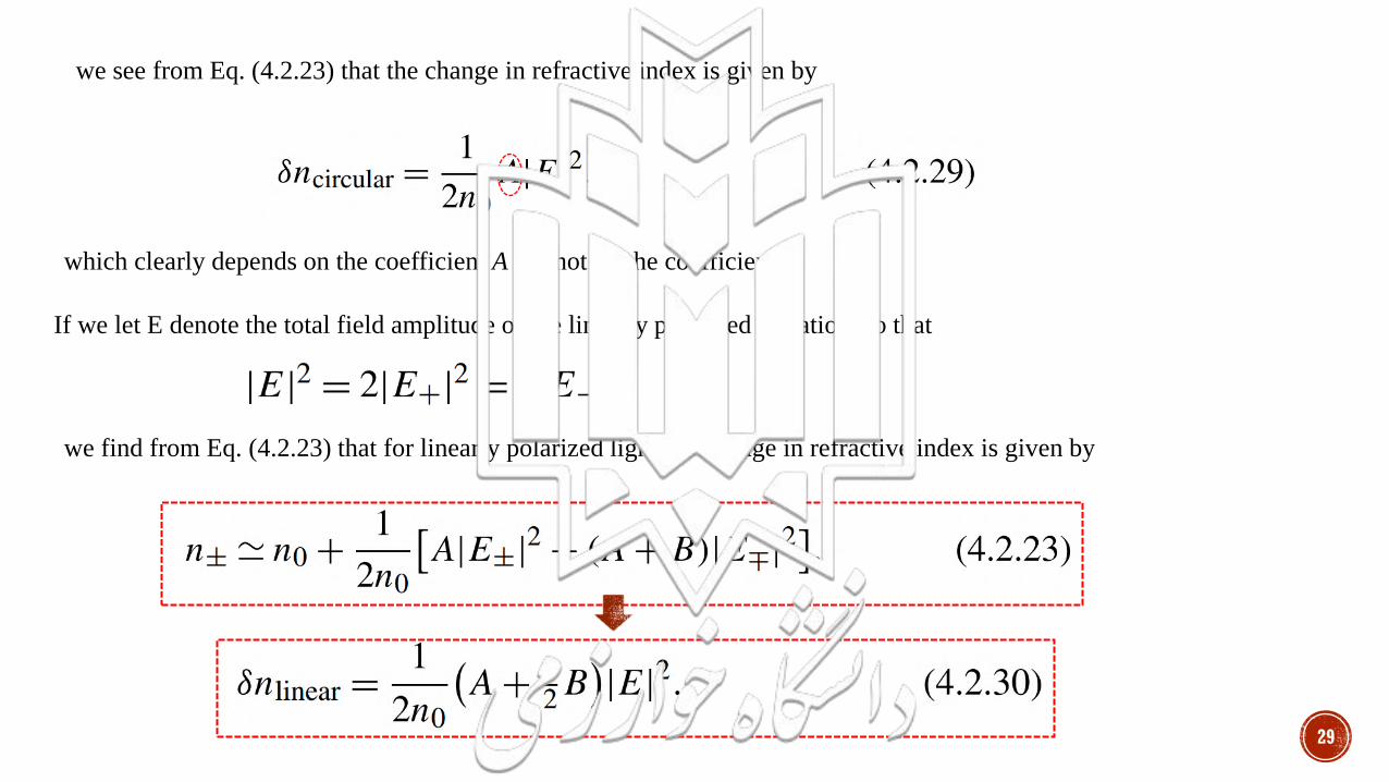
we see from Eq. (4.2.23) that the change in refractive index is given by
which clearly depends on the coefficient A but not on the coefficient B.
If we let E denote the total field amplitude of the linearly polarized radiation, so that
we find from Eq. (4.2.23) that for linearly polarized light the change in refractive index is given by
30
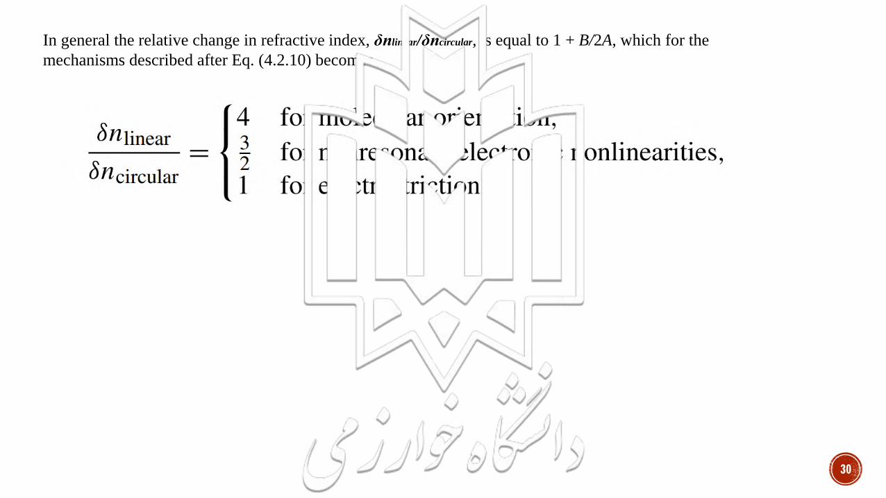
In general the relative change in refractive index, δnlinear/δncircular, is equal to 1 + B/2A, which for the
mechanisms described after Eq. (4.2.10) becomes

THE INTENSITY-DEPENDENT REFRACTIVE INDEX
▪ 4.1. Descriptions of the Intensity-Dependent Refractive Index
▪ 4.2. Tensor Nature of the Third-Order Susceptibility
▪ 4.3. Nonresonant Electronic Nonlinearities
▪ 4.4. Nonlinearities Due to Molecular Orientation
▪ 4.5. Thermal Nonlinear Optical Effects
▪ 4.6. Semiconductor Nonlinearities
▪ 4.7. Concluding Remarks
31
32
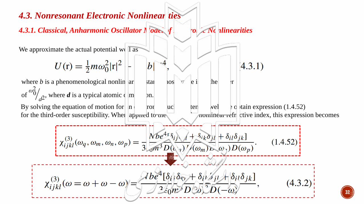
4.3. Nonresonant Electronic Nonlinearities
4.3.1. Classical, Anharmonic Oscillator Model of Electronic Nonlinearities
We approximate the actual potential well as
where b is a phenomenological nonlinear constant whose value is of the order
of ൘ω
02
d2, where d is a typical atomic dimension.
By solving the equation of motion for an electron in such a potential well, we obtain expression (1.4.52)
for the third-order susceptibility. When applied to the case of the nonlinear refractive index, this expression becomes
33
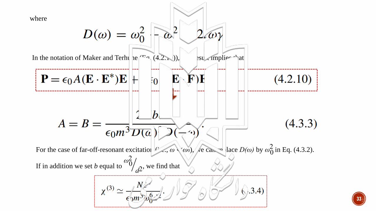
where
In the notation of Maker and Terhune (Eq. (4.2.10)), this result implies that
For the case of far-off-resonant excitation (i.e., ω ≪ω0), we can replace D(ω) by ω02 in Eq. (4.3.2).
If in addition we set b equal to ൘ω
02
d2, we find that
34
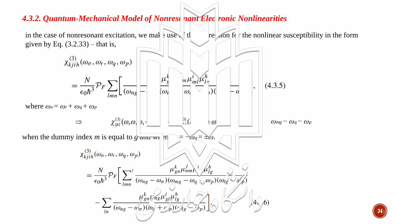
4.3.2. Quantum-Mechanical Model of Nonresonant Electronic Nonlinearities
in the case of nonresonant excitation, we make use of the expression for the nonlinear susceptibility in the form
given by Eq. (3.2.33) – that is,
where ωσ = ωr + ωq + ωp
(3) (3)( , , , ) ( )ijkl ijkl − = = + − ωmg − ωq − ωp
when the dummy index m is equal to g and when ωp = −ωq = ±ω.
35
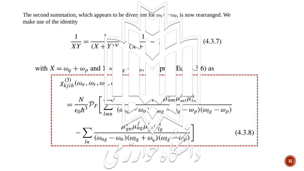
The second summation, which appears to be divergent for ωq = −ωp, is now rearranged. We
make use of the identity
36
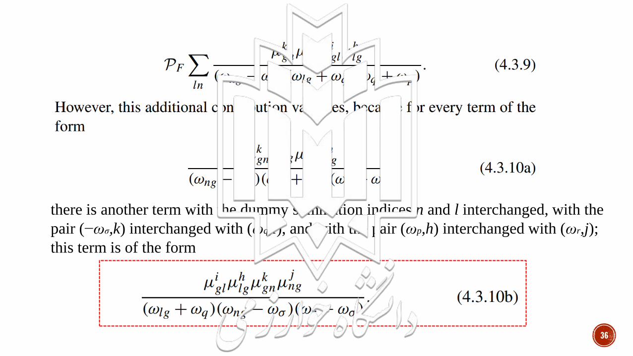
there is another term with the dummy summation indices n and l interchanged, with the
pair (−ωσ,k) interchanged with (ωq,i), and with the pair (ωp,h) interchanged with (ωr,j);
this term is of the form
37
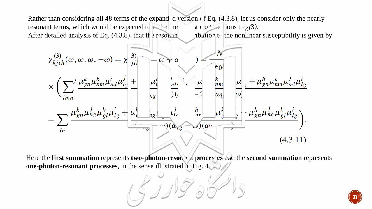
Rather than considering all 48 terms of the expanded version of Eq. (4.3.8), let us consider only the nearly
resonant terms, which would be expected to make the largest contributions to χ(3).
After detailed analysis of Eq. (4.3.8), that the resonant contribution to the nonlinear susceptibility is given by
Here the first summation represents two-photon-resonant processes and the second summation represents
one-photon-resonant processes, in the sense illustrated in Fig. 4.3.1.
38
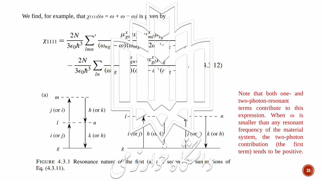
We find, for example, that χ1111(ω = ω + ω − ω) is given by
Note that both one- and
two-photon-resonant
terms contribute to this
expression. When ω is
smaller than any resonant
frequency of the material
system, the two-photon
contribution (the first
term) tends to be positive.
39
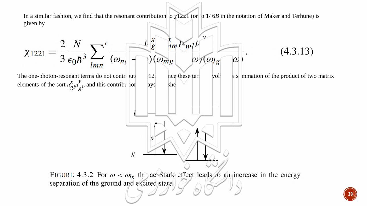
In a similar fashion, we find that the resonant contribution to χ1221 (or to 1/ 6B in the notation of Maker and Terhune) is
given by
The one-photon-resonant terms do not contribute to χ1221, since these terms involve the summation of the product of two matrix
elements of the sort μglx μ
gly
, and this contribution always vanishes.
40
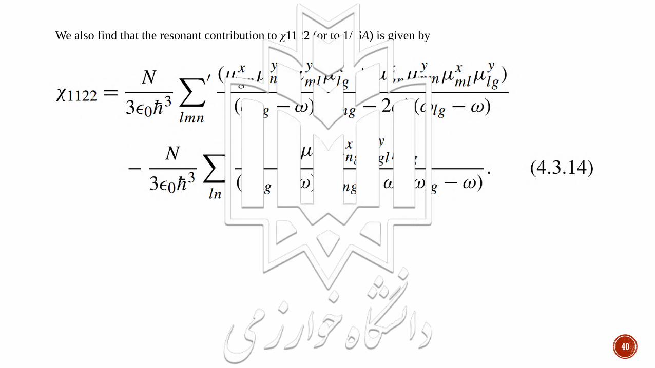
We also find that the resonant contribution to χ1122 (or to 1/ 6A) is given by
41
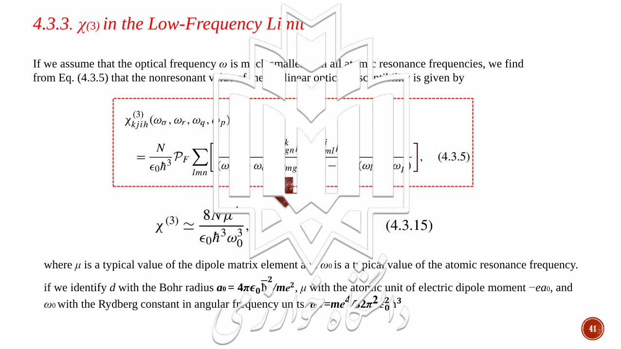
4.3.3. χ(3) in the Low-Frequency Limit
If we assume that the optical frequency ω is much smaller than all atomic resonance frequencies, we find
from Eq. (4.3.5) that the nonresonant value of the nonlinear optical susceptibility is given by
where μ is a typical value of the dipole matrix element and ω0 is a typical value of the atomic resonance frequency.
if we identify d with the Bohr radius a0 = 4π𝝐𝟎ħ𝟐/me𝟐, μ with the atomic unit of electric dipole moment −ea0, and
ω0 with the Rydberg constant in angular frequency units, ω0 =me4/32π2𝝐𝟎𝟐ħ𝟑
42
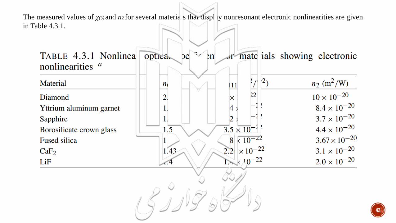
The measured values of χ(3) and n2 for several materials that display nonresonant electronic nonlinearities are given
in Table 4.3.1.

THE INTENSITY-DEPENDENT REFRACTIVE INDEX
▪ 4.1. Descriptions of the Intensity-Dependent Refractive Index
▪ 4.2. Tensor Nature of the Third-Order Susceptibility
▪ 4.3. Nonresonant Electronic Nonlinearities
▪ 4.4. Nonlinearities Due to Molecular Orientation
▪ 4.5. Thermal Nonlinear Optical Effects
▪ 4.6. Semiconductor Nonlinearities
▪ 4.7. Concluding Remarks
43