Embed Size (px)
Citation preview
[17:16 23/4/2016 rdv016.tex] RESTUD: The Review of Economic Studies Page: 1568 1568–1611
Review of Economic Studies (2015) 82, 1568–1611 doi:10.1093/restud/rdv016© The Author 2015. Published by Oxford University Press on behalf of The Review of Economic Studies Limited.Advance access publication 20 April 2015
The Institutional Causes ofChina’s Great Famine,
1959–1961XIN MENG
Australian National University
NANCY QIANYale University
and
PIERRE YAREDColumbia University
First version received January 2012; final version accepted January 2015 (Eds.)
This article studies the causes of China’s Great Famine, during which 16.5 to 45 million individualsperished in rural areas. We document that average rural food retention during the famine was too high togenerate a severe famine without rural inequality in food availability; that there was significant variancein famine mortality rates across rural regions; and that rural mortality rates were positively correlatedwith per capita food production, a surprising pattern that is unique to the famine years. We provideevidence that an inflexible and progressive government procurement policy (where procurement couldnot adjust to contemporaneous production and larger shares of expected production were procured frommore productive regions) was necessary for generating this pattern and that this policy was a quantitativelyimportant contributor to overall famine mortality.
Key words: Famines, Modern chinese history, Institutions, Central planning
JEL Codes: P2, O43, N45
1. INTRODUCTION
During the 20th century, approximately 70 million people perished from famine. This studyinvestigates the causes of the Chinese Great Famine (1959–1961), which killed more than anyother famine in history: 16.5 to 45 million individuals, most of whom were living in rural areas,perished in just over three years.1 The existing literature on the causes of the Great Famine hasformed a consensus that a fall in aggregate food production in 1959 followed by high governmentprocurement from rural areas were key contributors to the famine.2 In this article, we arguethat these factors could not have caused the famine on their own because average rural food
1. See Sen (1981) and Ravallion (1997) for estimates of total famine casualties. For the Chinese famine, mortalityestimates range from 16.5 million (Coale, 1981) to 30 million (Banister, 1987) to 45 million (Dikotter, 2010).
2. For more details, see the discussion at the end of Sections 1 and 2.
1568
at Colum
bia University L
ibraries on April 25, 2016
http://restud.oxfordjournals.org/D
ownloaded from
[17:16 23/4/2016 rdv016.tex] RESTUD: The Review of Economic Studies Page: 1569 1568–1611
MENG ET AL. INSTITUTIONAL CAUSES OF CHINA’S GREAT FAMINE 1569
availability was too high to generate famine, even after accounting for procurement. Thus, anyexplanation of the famine must account for inequality in food availability and famine mortalityacross rural areas. Motivated by this reasoning, we analyse the spatial relationship betweenagricultural productivity and famine severity. Using a panel of provinces, we find a surprisingpositive correlation between mortality rates and productivity across rural areas during the famine.We provide evidence that a procurement policy that was inflexible (i.e. procurement could notadjust to contemporaneous production) and progressive (i.e. procurement was a larger share ofexpected production in productive regions) was necessary for generating this pattern and that thispolicy was a quantitatively important contributor to overall famine mortality.
The goal of this study is to make progress on understanding the root causes of the famineby providing evidence for the novel hypothesis that the inflexibility of the centrally plannedprocurement system was an important contributing factor to the famine. Our study proceedsin several steps. The first step is to document that after procurement, rural regions as awhole retained enough food to avert mass starvation during the famine. Since the entire ruralpopulation relied on rural food stores, we compare the food retained by rural regions afterprocurement to the food required by rural regions to prevent famine mortality. Using historicaldata on aggregate food production, government procurement and population (adjusted for thedemographic composition), we find that average rural food availability for the entire ruralpopulation was almost three times as much as the level necessary to prevent high famine mortality.We reach these conclusions after constructing the estimates to bias against finding sufficientrural food availability. Our findings are consistent with Li and Yang’s (2005) estimates of highrural food availability for rural workers and imply that the high level of famine mortality wasaccompanied by significant variation in famine severity within the rural population.3 There musthave been some factor that caused a large rise in the inequality of access to food across the ruralpopulation, which, in turn, resulted in significant variance in mortality outcomes across the ruralpopulation.
The second step is to verify this conjecture by documenting that the increase in mortality ratesduring the famine was accompanied by an increase in the variance of mortality across the ruralpopulation. Since the historical mortality data are limited to total mortality at the regional level,we focus on spatial variation in mortality. We find that mortality rates across provinces variedmuch more during the famine than in other years. To investigate whether this pattern remainstrue at a more disaggregated level, we also use the birth cohort sizes of survivors observed in1990 to proxy for famine severity at the county level.4 This is based on the logic that famineincreases infant and early childhood mortality rates and lowers fertility rates such, that a moresevere famine results in smaller cohort sizes for those born shortly before or during the famine.The data show that there is much more variation in cross-county birth cohort sizes for faminebirth cohorts relative to non-famine birth cohorts. This is true both across and within provinces.These findings imply that an explanation of the famine that will need to account for the increasein both the mean and the variation of rural mortality rates.
Thirdly, we document the empirical relationship between mortality rates and productivityacross rural areas. We find that across rural regions, famine severity is positively correlated withper capita food production, a pattern that is unique to the famine era. This surprising correlationholds at the province level, where we use mortality rates to proxy for famine severity and percapita grain production data to measure productivity.
We acknowledge that these estimates could be biased by contemporaneous misreporting ofthe historical data for production and mortality. For example, the Chinese government during the
3. We compare Li and Yang’s (2005) estimates to ours at the end of Section 3.4. There are no county level historical data on mortality rates or food production.
at Colum
bia University L
ibraries on April 25, 2016
http://restud.oxfordjournals.org/D
ownloaded from
[17:16 23/4/2016 rdv016.tex] RESTUD: The Review of Economic Studies Page: 1570 1568–1611
1570 REVIEW OF ECONOMIC STUDIES
Great Leap Forward era (GLF 1958–1961) was known to have over-reported grain production.Hence, one may be concerned that the positive correlation between mortality and reportedproduction reflects the over-reporting of production in the more famine-stricken regions. Toaddress this, we impute production with data that were not known to have been manipulated,such as historical weather conditions and geo-climatic suitability, and data that would have beeneasy to correct after the GLF, such as total rural population and total land area. To minimizethe possibility that our results are driven by misreporting, the main empirical analysis of thespatial patterns uses the constructed production measure. Moreover, at the county level, we showthat famine survivor cohort sizes are negatively correlated with the predictors of high grainproductivity (e.g. geo-climatic suitability for grain production, rainfall, and temperature).
The fourth step is to examine whether our empirical findings can be explained by existingtheories of the causes of the famine, which have primarily focused on the role that policies specificto the GLF played in causing the famine. We take the variables for GLF policies used in existingstudies and show that regional GLF intensity cannot explain the patterns we observe in the dataand a new explanation is needed. Moreover, we show that productivity explains much more ofthe variation in the mortality increase during the famine than GLF intensity. Thus, explaining thecorrelation between productivity and famine severity across rural areas can potentially explain alarge fraction of overall famine mortality.
Finally, we provide an explanation for the empirical findings. We argue that the spatial patternsof famine severity were the result of an inflexible and progressive government procurement policycombined with a fall in per capita production that was typically larger in magnitude in moreproductive regions, but not so large that it changed productivity ranks across provinces. In thelate 1950s, the central government procured as much grain as it could from rural areas whileleaving rural workers with enough food to be productive labourers. It was thus progressive asit procured a higher percentage of total production from productive areas. It was also inflexibleas the government set each region’s procurement level in advance such that it could not beeasily adjusted afterward. This was because weak state capacity, along with political tensions,made communication challenging and hampered the government’s ability to respond quickly toa harvest that was below expectations. As a consequence, the level of procurement from a givenrural region did not respond to the actual amount produced, but was instead based on an estimatedproduction target established earlier, where this target was itself based on past production. Afterprocurement took place, the food retained in a given region would be negatively correlatedwith the difference between target production and realized production, that is, the “productiongap”. Since more productive regions experienced a larger absolute production drop while stillremaining more productive relative to less productive regions, the procurement policy causedmore productive regions to experience a larger per capita production gap, subjecting them tomore over-procurement, which in turn, led to less per capita food retention, less per capita foodconsumption, and higher mortality rates.
To examine the plausibility of our explanation, we test the prediction of our proposedmechanism that mortality rates should be positively correlated with the production gap and thatthis should be true in all years during the 1950s and 1960s since they were subject to a similarprocurement policy. To estimate the production gap, we construct a measure of target productionthat is based on past production and past production growth. The results show that provincelevel mortality is positively associated with the production gap, a relationship that is robust tocontrolling for GLF intensity.
A back-of-the-envelope calculation shows that the inflexible and progressive procurementmechanism explains 32–43% of total famine mortality. Hence, our proposed mechanism isquantitatively important, and at the same time leaves room for other factors, such as GLF policiesand the complex political environment of the time, to contribute to famine mortality.
at Colum
bia University L
ibraries on April 25, 2016
http://restud.oxfordjournals.org/D
ownloaded from
[17:16 23/4/2016 rdv016.tex] RESTUD: The Review of Economic Studies Page: 1571 1568–1611
MENG ET AL. INSTITUTIONAL CAUSES OF CHINA’S GREAT FAMINE 1571
In addition, we use historical province level procurement data to provide evidence on thecausal links of our hypothesis. For example, we document that during the famine, the positivecorrelation between regional procurement rates and productivity increases, and regional foodretention, which is the difference between production and procurement, is decreasing in the sizeof the production gap.
The main challenges for our study are data availability and quality. We address these difficultiesby using a large array of data from contemporaneous, archival, Chinese, and international sources.As we discussed earlier, we address the possibility of systematic over-reporting of production byconstructing a measure of production that does not use GLF-era production data. We are also ableto address potential concerns that mortality rates are misreported by proxying for famine severitywith survivor birth cohort size as observed in 1990. The fact that the results are qualitativelysimilar across all data sources suggests that the spatial patterns we detect between agriculturalproductivity and famine severity are not driven by measurement error.
This study makes progress on understanding the causes of the Chinese famine in severalways. First, it is the first to propose that an inflexible and progressive procurement policy wasan important contributing factor of the famine, and the first to document the surprising positiveassociation between famine mortality rates and agricultural productivity. Secondly, it is one of thefew studies that examine the determinants of regional procurement (most existing studies treatprocurement as an exogenous variable). Since government procurement is a key determinant ofregional food retention, and we show that inequality in food retention across regions is necessaryfor causing a large famine, understanding the determinants of regional procurement levels (i.e. theinequality in procurement across regions) is critical for understanding the famine. Another studythat examines the determinants of regional procurement levels is Kung and Chen (2011). Theyfind that political radicalism increased regional procurement during the famine and explainsapproximately 16% of total famine mortality. As such, our mechanism complements theirs inexplaining total famine mortality. Finally, to the best of our knowledge, we are also the first toaddress potential measurement error in the GLF-era grain production data. Past studies have takenthe official production data as given.
In directly examining the determinants of mortality, our study is similar to Lin and Yang(2000), which finds that conditional on average grain production, lower grain production (andhigher urban population share) that were associated with higher mortality during the famine.That a decline in production relative to a region’s average production leads to higher mortality isconsistent with our inflexibility mechanism. In another study of famine mortality, Kung and Lin(2003) finds that conditional on procurement, higher production is associated with lower mortality,and that conditional on production, lower procurement is associated with lower mortality. Relatedto this, Li and Yang (2005) finds that during the famine, lower food retention (production minusprocurement) and zealousness in pursuing GLF policies lead to lower food production in thefollowing year. Our finding that food retention is negatively associated with famine is consistentwith these earlier studies.
This study also adds to the larger literature on famines. Our results are broadly consistent withSen (1981)’s thesis that famines are mainly due to food distribution rather than aggregate fooddeficits. However, we document spatial patterns in famine severity and food production that aredifficult to explain with market mechanisms.5 Thus, together with other studies of the Chinesefamine, we expand the literature on the causes of famine by studying the detailed mechanisms in
5. For example, Sen (1981) found that the Bengal Famine (1943) was partly due to the inability of rural wageworkers in famine stricken regions to buy food from regions with surplus production. With such a mechanism, mortalityrates would be higher in less productive regions.
at Colum
bia University L
ibraries on April 25, 2016
http://restud.oxfordjournals.org/D
ownloaded from
[17:16 23/4/2016 rdv016.tex] RESTUD: The Review of Economic Studies Page: 1572 1568–1611
1572 REVIEW OF ECONOMIC STUDIES
a non-market context.6 This is an important context since over 60% of all famine deaths in the20th century taken place in non-market economies (e.g. China’s Great Famine in 1959–1961, theSoviet Famine in 1932–1933, and the North Korean Famine in 1992–1995).7 In the Conclusion,we discuss the similarities between the Chinese famine and famines in other centrally plannedeconomies.
This article is organized as follows. Section 2 provides a brief historical background. Section 3estimates rural food availability during the famine. Section 4 documents spatial variation in famineseverity. Section 5 estimates the correlation between famine severity and food productivity acrossrural regions. Section 6 explains the empirical patterns with the inflexibility and progressivenessof the historical food procurement policy. Section 7 offers concluding remarks.
2. BACKGROUND
In this section, we provide a brief discussion about the historical background of the famine.For more detailed discussions, please see our earlier working paper, Meng et al. (2010), and thereferences below.
2.1. Collective agriculture
On the eve of the famine, the production, distribution, and consumption of food in China wereentirely controlled by the central government. This meant that the government was the sole insurerof food consumption in the event of a drop in production.8 At the time, approximately 80% ofthe population worked in agriculture.9 Land reforms that began in 1952 had resulted in fullcollectivization by the end of the decade. Private property rights to land and assets were erased,and markets for private transactions were banned (Fairbank, 1987: p. 281–285). Agriculturalworkers were forced to work under constant monitoring and were no longer rewarded for theirmarginal input into production (Johnson, 1998). By the end of the 1950s, there were no wages orcash rewards for effort.10
Grain was harvested and stored communally. Private stores of grain were banned, a rulethat was sometimes enforced with virulent anti-hiding campaigns (Becker, 1996: p. 109). Grainwas procured by the central government from communal depots after the fall harvest aroundNovember. Procured grain was fed to urban workers, exported to other countries in exchange forindustrial equipment and expertise, and stored in reserves as insurance against natural disaster.11
The grain retained by rural regions was fed to peasants in communal kitchens, which wereestablished so that the collective controlled food preparation and consumption. The government
6. For recent studies on the causes of famines in market economies, see studies such as Burgess and Donaldson(2010), (Shiue, 2002, 2004, 2005) and OGrada (2007). Also, Dreze (1999) and OGrada (2007) provide overviews ofthis literature. See Section 2 for a discussion on studies of the famine in China besides the ones that we have alreadymentioned.
7. Davies and Wheatcroft (2004) estimate that up to 6.5 million died across the Soviet Union during the 1932famine. In North Korea, it is commonly believed that 2–3 million individuals, approximately 10% of the total population,died during this famine (e.g. see Haggard and Noland, 2005; Demick, 2009). There are very few academic studies orreliable accounts of details related to this famine.
8. See the previous version of this article, Meng et al. (2010), for a detailed discussion on how agriculturalcollectivization during the 1950s reduced rural households’ ability to smooth consumption.
9. We calculate this from data reported by the National Bureau of Statistics (NBS).10. See Walker, 1965 (p. 16–17) for a detailed description of collectivization.11. Historical central planning documents state that approximately 4–5 million tons per year were put into reserves
as insurance against natural disasters (Sun, 1958). During the late 1950s, total grain exports were approximately 2% oftotal production (Walker, 1984: Table 52).
at Colum
bia University L
ibraries on April 25, 2016
http://restud.oxfordjournals.org/D
ownloaded from
[17:16 23/4/2016 rdv016.tex] RESTUD: The Review of Economic Studies Page: 1573 1568–1611
MENG ET AL. INSTITUTIONAL CAUSES OF CHINA’S GREAT FAMINE 1573
prevented peasants from migrating, and thus, peasants could only eat from the amount distributedto their collective (Thaxton, 2008: p. 166). When that was insufficient, famine occurred.
2.2. Famine chronology
The Great Famine is officially defined by the Chinese government to be three years, 1959–1961,when mortality rates were the highest. Grain production grew nearly monotonically between1949 and 1957. There are a few accounts of production falls in select regions in 1958 and manyaccounts of widespread production falls in 1959 and 1960. Famine became widespread when localstores of the 1959 harvest ran out during the early part of 1960 (Thaxton, 2008: p. 207–210).Between 16.5 and 45 million individuals died during the three years in total.12 Mortality rateswere the highest in the spring of 1960 (Becker, 1996: p. 94).13 The official explanation providedby the government was bad weather. Recent studies have provided evidence that the fall in outputwas also partly due to bad government policies such as the diversion of resources away fromagriculture to industrialization, as well as weakened worker incentives.14
Famine primarily struck the rural areas. Communal kitchens, which survivors recall as havingserved large quantities of food, suddenly ran out. Peasants scavenged for calories and ate greencrops illegally from the field (chi qing) when they could (Thaxton, 2008: p. 202). Mortality rateswere highest for the elderly and young children (Ashton et al. 1984: Tables 3 and A7; Spence,1990: p. 583). Prime-age adults experienced relatively higher survival rates (Thaxton, 2008:p. 202–210).
Relative to other famines, infectious diseases did not play a major role in causing mortality.The low level of disease in rural areas during the famine has been attributed to limited populationmovements, the prevalent use of DDT before the famine, and public health measures taken bythe government during earlier years (e.g. Fairbank, 1987: p. 279; Becker, 1996; Dikotter, 2010:ch. 32). “People really did die of starvation—in contrast to many other famines where diseaseloomed large on the horizon of death” (Dikotter, 2010: p. 285). This is an important point to keepin mind for calculating the caloric requirement for survival in the Chinese context.15
In recent years, a broad consensus has formed that the government over-procured grainfrom rural areas in the fall of 1959, and this exacerbated the production decline and causedthe massive mortality in the spring months of 1960. There are many hypotheses for what led toover-procurement. The central government placed the blame on local leaders, accusing them ofover-reporting production and consequently leading the central government to over-estimate trueproduction (Thaxton, 2008: p. 293–9). Recent academic studies find that over-procurement was
12. For example, mortality estimates range from 16.5 million (Coale, 1981) to 30 million (Banister, 1987) to 45million (Dikotter, 2010).
13. See the Section 1 for references to studies of total famine mortality. For example, “By the end of 1959, muchof the peasantry was starving to death but the hardest time in the entire famine came in January and February when thegreatest number perished” (Becker, 1996: p. 94).
14. The policies include labour and acreage reductions in grain production (e.g. Peng, 1987; Yao, 1999),implementation of radical programs such as communal dining (e.g. Chang and Wen, 1997; Yang, 1998), reduced workincentives due to the formation of the people’s communes (Perkins and Yusuf, 1984), and the denial of peasants’ rightsto exit from the commune (Lin, 1990). Li and Yang (2005) compile province level panel data on grain production andattempt to quantify the impact of various potential factors. They find that in addition to weather, the relevant factors wereover-procurement and the diversion of labour away from agriculture during the Great Leap Forward for projects such asrural industrialization.
15. Consistent with the belief that infectious diseases were not an important feature of the Chinese Famine, the datashow that famine mortality rates were low in densely populated places such as urban areas and were uncorrelated withlatitude and elevation. Moreover, the results we show in the article are robust to controlling for population density andits interaction with the famine dummy variable. These correlations are available upon request.
at Colum
bia University L
ibraries on April 25, 2016
http://restud.oxfordjournals.org/D
ownloaded from
[17:16 23/4/2016 rdv016.tex] RESTUD: The Review of Economic Studies Page: 1574 1568–1611
1574 REVIEW OF ECONOMIC STUDIES
driven by multiple factors, including the government’s bias towards providing high levels of foodto urban areas (Lin and Yang, 2000), the political zealousness and career concerns of provincialleaders (Yang, 1998; Kung and Chen, 2011), and an over-commitment by the central governmentto meeting export targets (Johnson, 1998). In addition, some have argued that mortality rates wereexacerbated by food wastage in communal kitchens (Chang and Wen, 1997).
The Chinese government did not begin to systematically respond to the famine until thesummer of 1960, after a large proportion of famine mortality had already taken place. The responsecame in several forms. The government returned workers who had been recently moved to urbanareas to assist in industrialization back to their home villages. This was intended to replenishthe greatly weakened and demoralized rural labour force to minimize further falls in production(Li and Yang, 2005; Thaxton, 2008: p. 169). Urban food rations were reduced, although typicallynot to below subsistence levels (Lin and Yang, 2000). The government also abandoned many ofthe more extreme policies of collectivization (Walker, 1965: p. 83, 86–92; Thaxton, 2008: ch. 6,p. 215–216). For example, households again stored and prepared their own food, peasants wereagain allowed to plant strips of sweet potatoes for their own consumption, and the governmentsometimes also turned a blind eye to the black market trading of food across regions and theillegal consumption of green crops; all this helped preserve lives until the next harvest (Thaxton,2008: ch. 4).
These measures could not prevent another decline in production in 1960, this time caused bythe diminished physical capacity of the rural labour force, the lack of organic inputs such as seedsand fertilizers, which had been consumed during the months of deprivation (e.g. Li and Yang,2005), and the consumption by starving peasants of green crops from the field (Thaxton, 2008:p. 202). In 1961, the government finally ended the famine by sending large amounts of grain intorural areas. Thirty million tons of grain reserves were depleted (Walker, 1984: Ch. 5) and Chinaswitched from being a net exporter to a net importer of grain (Walker, 1984: Table 52). Grainproduction recovered gradually in subsequent years.
After the famine, procurement rates were kept at a much lower level than during the famineera. Official statistics show that aggregate procurement rates gradually declined from a peak ofalmost 30% of total production in 1960 to approximately 10% by 1965, and remained between 6%and 19% for the next 20 years.16 The procurement policy remained largely unchanged otherwise.Consistent with the low procurement levels and the government’s need to feed its growing urbanpopulation, China remained a net importer of grain for several decades. The government did notattempt to re-implement the extreme policies from the GLF that were abandoned during the initialreaction to the famine. China experienced several aggregate production drops of approximately5–10% in per capita terms, but never experienced another fall as large as that of 1959 (i.e. 15%).These factors, together, may explain why there were no subsequent famines in China (Walker,1965: ch. 6; Thaxton, 2008: ch. 6).
Politically, the central government engaged in various public campaigns to preserve politicalsupport during the famine’s aftermath. This was necessary since the famine had primarilyaffected the rural population which represented the support base of the communist regime. Thegovernment limited the reports of famine and minimized the mortality numbers; it initiated large-scale propaganda campaigns such as yiku sitan to convince the population that bad weather andcorrupt bureaucrats were to blame for low production and over-procurement; and it initiated the
16. Note that the aggregate procurement rates discussed in the next section and displayed in Table 1 differ slightlyfrom the national average. This is because our analysis utilizes a restricted sample of provinces. All of our results areunchanged if one uses the full sample (as we do in a previous version of this article) or the restricted sample. Resultsusing the full sample are available upon request.
at Colum
bia University L
ibraries on April 25, 2016
http://restud.oxfordjournals.org/D
ownloaded from
[17:16 23/4/2016 rdv016.tex] RESTUD: The Review of Economic Studies Page: 1575 1568–1611
MENG ET AL. INSTITUTIONAL CAUSES OF CHINA’S GREAT FAMINE 1575
fan wufeng movement to allow peasants to punish local leaders for famine crimes (Thaxton, 2008:p. 293–299).
Our study focuses on the three years of the highest mortality rates, 1959–1961. Since themid-autumn harvest is used to support life for many months of the following year, we focus ongrain production during 1958–1960. The chronology of production and mortality rates portraya consistent picture, where roughly constant levels of production in 1958 led to above-trendmortality rates in 1959, and bigger falls in production in 1959 led to extremely high mortalityrates in 1960. Per capita production was similar during 1960–1961, during which time mortalityrates declined. Per capita production began to grow in 1962, at which point mortality rates returnedto trend. We document these facts explicitly in the next sections.
3. RURAL FOOD AVAILABILITY
We argue in this section that rural areas retained enough food post-procurement to avoid mortality.In this endeavour, we consistently bias our exercise in the direction of overestimating the foodshortage. The main analysis uses a sample of 19 of the 24 provinces in China during the famineera. For these provinces, we have data for all of the main variables used in the analysis: mortality,urban, and rural population, production, procurement, weather, and geographical conditions. Forconsistency, we use the same sample for all of the estimates presented in the main article. Oursample comprises 77% of China’s total population in 1958 and approximately 87% of total faminemortality.17
3.1. Rural caloric requirements
To calculate rural food availability when the famine began, we compare production to per capitacaloric requirements. The main exercise uses official production data, but we later show thatthe main result is robust to using constructed measures of production. We focus on a seven-year window that includes the three official years of famine, 1959–1961. Mortality rates during1959–1961 depend on the consumption of food produced during 1958–1960 since harvests areused to support life for a large part of the following calendar year and only a small part of thecurrent calendar year.
We calculate two benchmarks for caloric requirements: the caloric needs for heavy adult labourand healthy child development and the caloric needs for staying alive. We use very generouscaloric recommendations provided by the U.S. Department of Agriculture (USDA) for the firstbenchmark, and we calculate the lower benchmark to be 43% of the higher one.18 To adjust
17. The provinces in our sample are Anhui, Beijing, Fujian, Guangdong, Hebei, Heilongjiang, Henan, Hubei,Hunan, Jiangsu, Jiangxi, Jilin, Liaoning, Shaanxi, Shandong, Shanghai, Shanxi, Tianjin, and Zhejiang. Famine mortalitywas calculated by the authors using mortality data reported by the National Bureau of Statistics. In this instance, it isdefined as the deaths during the famine that was in excess to the average level of mortality during the six years prior toand five years after the famine (1953–1958, 1962–1966). Please see the Online Appendix available as SupplementaryData for a detailed discussion.
18. There is little evidence for how many calories are needed to stay alive. This is partly because starvation istypically accompanied by other conditions such as disease, unsanitary conditions, war, etc. All of these other factorscontribute to mortality, but they are less applicable in our context than for most other famines since rural China had alow level of endemic disease, had high sanitary standards, and did not experience war. The best evidence we have oncalories and starvation is from the Minnesota Starvation Experiment, where the U.S. military systematically subjectedmilitary volunteers to high levels of physical exertion, chronic starvation, and harsh conditions (e.g. high temperatures).In these experiments, the lowest level of caloric consumption was approximately 900 calories a day. This was far abovethe level that would cause mortality and the subjects were still required to exercise. Similarly, Dasgupta and Ray (1986),
at Colum
bia University L
ibraries on April 25, 2016
http://restud.oxfordjournals.org/D
ownloaded from
[17:16 23/4/2016 rdv016.tex] RESTUD: The Review of Economic Studies Page: 1576 1568–1611
1576 REVIEW OF ECONOMIC STUDIES
for the demographic structure, we use the published tables extracted from the 1953 PopulationCensus. Thus, we assume that the per capita food requirement in 1959 is similar to that of 1953. Inthe Online Appendix available as Supplementary Data, we describe how we apply demographicdata to the USDA guidelines to calculate the average per capita caloric needs for the population.We estimate that daily average per capita requirements in 1959 were 1871 calories for the firstbenchmark and 804 for the second benchmark. These estimates are lower than average caloricrequirements for adult workers because they also account for young and elderly individuals inthe population, who require fewer calories per person. It is important to note that our estimatesare extremely conservative and constructed to obtain high levels of caloric requirement.
The main caveat in interpreting these estimates is that the demographic structure may havechanged between 1953 and 1959 such that per capita requirements were higher in 1959. Thisis unlikely because the proportion of prime-age adults in the population decreased during1953–1959.19 Since the very young and elderly require fewer calories than prime-age adults,this would most likely cause us to over-estimate average per capita caloric needs in 1959.
Applying the 1953 estimates to the years immediately after the famine is more problematic.Since the young and the elderly were more likely to have perished during the famine, the averageper capita caloric needs during the post-famine years could have been much higher than in 1953.Hence, the caloric accounting for the years after the famine should be interpreted cautiously.
3.2. Rural food availability
Grain production, total population, and urban population data are published by the NBS. Thethree province level municipalities were mostly urban, but still contained significant agriculturalpopulations that engaged in grain production.20
The data on grain production is not disaggregated by types, which include rice, sorghum,and wheat. Therefore, to convert data for the volume of retained grain into calories, we use theChinese Ministry of Health and Hygiene’s (MHH) estimate of calories contained in the typicalmix of grains consumed by an average Chinese worker, and we assume that one kilogram of grainprovides 3587 calories. Moreover, we assume that individuals subsist solely on grain, which is areasonable description of the diet of Chinese peasants in the 1950s (Walker, 1984).
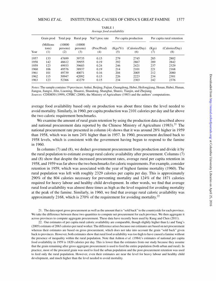
The data for national grain production and total population are displayed in Table 1 columns(1) and (2). In column (5), we use these data to estimate per capita production, which is thenconverted in column (6) into per capita food availability in terms of calories per day using theMHH’s estimate of calories per kilogram of grain. Aggregate production in column (1) andestimated per capita food availability in column (6) show that per capita production was roughlyconstant between 1957 and 1958. And although production and food availability declined from1958 to 1959, national production provided approximately 2421 calories per capita in 1959, whichis approximately 300% of the 804 calories necessary for preventing mortality and 129% of the1871 calories required for heavy labour and healthy child development. In other words, national
in their well-known paper on nutrition and work, chose the 900 calories per day benchmark as the amount required foran adult male to do some work. For these reasons, we also chose 900 calories as the lower benchmark and interpret it asthe extreme upper bound of the amount of calories required to survive. Since 900 calories is 43% of the level needed forheavy adult labour for prime-age men, we assume the same proportional needs for all other groups.
19. Crude demographic projections suggest that between 1953 and 1959, youth dependency (the number of peopleaged 0–10 per 100 people aged 20–64) approximately increased from 90 to 100. The rate of increase was constant overtime and shows no change during the GLF. Similarly, the dependency ratio of the elderly (the number of people over 64per 100 people aged 20–64) was constant over this period. These statistics suggest that the proportion of prime-age adultsin the population was declining (Kinsella et al. 2009).
20. During the 1950s, 34, 30, and 47% of the populations of Beijing, Shanghai, and Tianjin were rural.
at Colum
bia University L
ibraries on April 25, 2016
http://restud.oxfordjournals.org/D
ownloaded from
[17:16 23/4/2016 rdv016.tex] RESTUD: The Review of Economic Studies Page: 1577 1568–1611
MENG ET AL. INSTITUTIONAL CAUSES OF CHINA’S GREAT FAMINE 1577
TABLE 1Average food availability
Grain prod Total pop Rural pop Nat’l proc rate Per capita production Per capita rural retention
(Millions (10000 (10000tons) persons) persons) (Proc/Prod) (Kgs/Yr) (Calories/Day) (Kgs) (Calories/Day)
Year (1) (2) (3) (4) (5) (6) (7) (8)
1957 133 47699 39735 0.15 279 2745 285 28021958 142 48612 39955 0.19 292 2867 289 28421959 123 49933 39603 0.24 246 2421 237 23291960 106 49576 38937 0.19 214 2101 221 21681961 101 49739 40071 0.16 204 2005 212 20801962 115 50947 42092 0.15 226 2223 234 23011963 123 52366 43279 0.15 234 2303 242 2376
Notes: The sample contains 19 provinces:Anhui, Beijing, Fujian, Guangdong, Hebei, Heilongjiang, Henan, Hubei, Hunan,Jiangsu, Jiangxi, Jilin, Liaoning, Shaanxi, Shandong, Shanghai, Shanxi, Tianjin, and Zhejiang.Sources: CDSM50 (1999), CPIRC (2000), the Ministry of Agriculture (1983) and the authors’ computations.
average food availability based only on production was about three times the level needed toavoid mortality. Similarly, in 1960, per capita production was 2101 calories per day and far abovethe two caloric requirement benchmarks.
We examine the amount of rural grain retention by using the production data described aboveand national procurement data reported by the Chinese Ministry of Agriculture (1983).21 Thenational procurement rate presented in column (4) shows that it was around 28% higher in 1959than 1958, which was in turn 24% higher than in 1957. In 1960, procurement declined back to1958 levels, which is consistent with the government having begun to respond to the faminein 1960.
In columns (7) and (8), we deduct government procurement from production and divide it bythe rural population to estimate average rural caloric availability after procurement. Columns (7)and (8) show that despite the increased procurement rates, average rural per capita retention in1958, and 1959 was far above the two benchmarks for caloric requirements. For example, considerretention in 1959, which was associated with the year of highest famine mortality (1960). Therural population was left with roughly 2329 calories per capita per day. This is approximately290% of the 804 calories necessary for preventing mortality and 124% of the 1871 caloriesrequired for heavy labour and healthy child development. In other words, we find that averagerural food availability was almost three times as high as the level required for avoiding mortalityat the peak of the famine. Similarly, in 1960, we find that average rural caloric availability wasapproximately 2168, which is 270% of the requirement for avoiding mortality.22
21. The data report gross procurement as well as the amount that is “sold back” to the countryside for each province.We take the difference between these two quantities to compute net procurement for each province. We then aggregate itacross provinces to compute aggregate procurement. These data have recently been used by Kung and Chen (2011).
22. Our estimates of per capita rural caloric availability are comparable, though slightly higher than Li and Yang’s(2005) estimate of 2063 calories per rural worker. The difference arises because our estimates are based on net procurementwhereas their estimates are based on gross procurement, which does not take into account the grain “sold back” givenback to provinces. However, both estimates show that rural food availability was too high to have caused a famine withoutthe presence of inequality within the rural population. Note that Ashton et al. (1984)’s estimates of national per capitafood availability in 1959 is 1820 calories per day. This is lower than the estimates from our study because they assumethat the grain remaining after gross aggregate procurement is used to feed the entire population (both urban and rural). Inpractice, most of the procured grain was used to feed the urban population and the post-procurement retention was usedto feed only the rural population. However, even their estimates are near the level for heavy labour and healthy childdevelopment, and much higher than the level needed to avoid mortality.
at Colum
bia University L
ibraries on April 25, 2016
http://restud.oxfordjournals.org/D
ownloaded from
[17:16 23/4/2016 rdv016.tex] RESTUD: The Review of Economic Studies Page: 1578 1568–1611
1578 REVIEW OF ECONOMIC STUDIES
The main caveat for interpreting these estimates is that official data may overstate productionto minimize the appearance of failure of GLF agricultural policies, or to understate procurement tominimize government culpability. However, such misreporting is unlikely to overturn our resultthat aggregate rural retention exceeded aggregate rural nutritional needs for avoiding faminefor several reasons. First, we have followed recent studies on the famine in using productionand procurement data that was corrected and reported during the post-Mao reform era, whenthe government had no incentive to glorify or undermine the GLF. Secondly, we have madeassumptions throughout the exercise to bias our calculations towards finding low rural foodavailability (and high food requirements). Thirdly, for aggregate procurement to cause aggregaterural retention to be below the nutritional needs for avoiding famine mortality, procurementwould have needed to be 73% of total production in 1959, 70% in 1960, and 65% in 1961.These are three to four times the reported procurement rates and seem unlikely as there areno documented accounts of such drastic under-reporting of procurement. Finally, in the OnlineAppendix Section G available as Supplementary Data, we show that our finding changes littleif we use constructed production measures, which we describe in Section 5.1, and reasonableupper-bound values for procurement.
4. SPATIAL VARIATION IN FAMINE MORTALITY
4.1. Across provinces
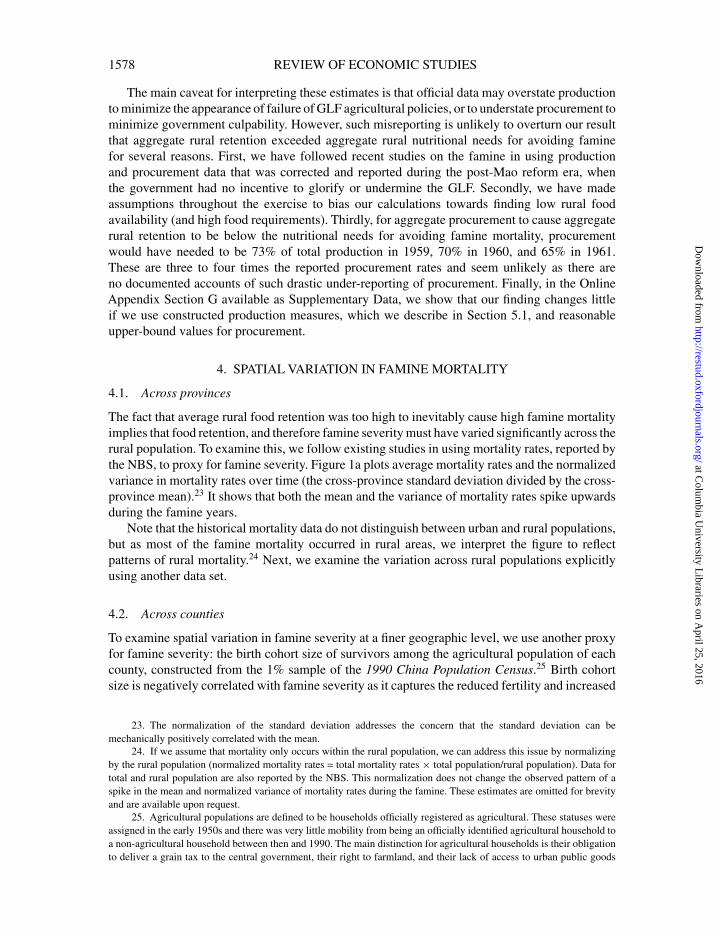
The fact that average rural food retention was too high to inevitably cause high famine mortalityimplies that food retention, and therefore famine severity must have varied significantly across therural population. To examine this, we follow existing studies in using mortality rates, reported bythe NBS, to proxy for famine severity. Figure 1a plots average mortality rates and the normalizedvariance in mortality rates over time (the cross-province standard deviation divided by the cross-province mean).23 It shows that both the mean and the variance of mortality rates spike upwardsduring the famine years.
Note that the historical mortality data do not distinguish between urban and rural populations,but as most of the famine mortality occurred in rural areas, we interpret the figure to reflectpatterns of rural mortality.24 Next, we examine the variation across rural populations explicitlyusing another data set.
4.2. Across counties
To examine spatial variation in famine severity at a finer geographic level, we use another proxyfor famine severity: the birth cohort size of survivors among the agricultural population of eachcounty, constructed from the 1% sample of the 1990 China Population Census.25 Birth cohortsize is negatively correlated with famine severity as it captures the reduced fertility and increased
23. The normalization of the standard deviation addresses the concern that the standard deviation can bemechanically positively correlated with the mean.
24. If we assume that mortality only occurs within the rural population, we can address this issue by normalizingby the rural population (normalized mortality rates = total mortality rates × total population/rural population). Data fortotal and rural population are also reported by the NBS. This normalization does not change the observed pattern of aspike in the mean and normalized variance of mortality rates during the famine. These estimates are omitted for brevityand are available upon request.
25. Agricultural populations are defined to be households officially registered as agricultural. These statuses wereassigned in the early 1950s and there was very little mobility from being an officially identified agricultural household toa non-agricultural household between then and 1990. The main distinction for agricultural households is their obligationto deliver a grain tax to the central government, their right to farmland, and their lack of access to urban public goods
at Colum
bia University L
ibraries on April 25, 2016
http://restud.oxfordjournals.org/D
ownloaded from
[17:16 23/4/2016 rdv016.tex] RESTUD: The Review of Economic Studies Page: 1579 1568–1611
MENG ET AL. INSTITUTIONAL CAUSES OF CHINA’S GREAT FAMINE 1579
(a)
(b)
—
—
Figure 1
Average and spatial variation in famine severity
at Colum
bia University L
ibraries on April 25, 2016
http://restud.oxfordjournals.org/D
ownloaded from
[17:16 23/4/2016 rdv016.tex] RESTUD: The Review of Economic Studies Page: 1580 1568–1611
1580 REVIEW OF ECONOMIC STUDIES
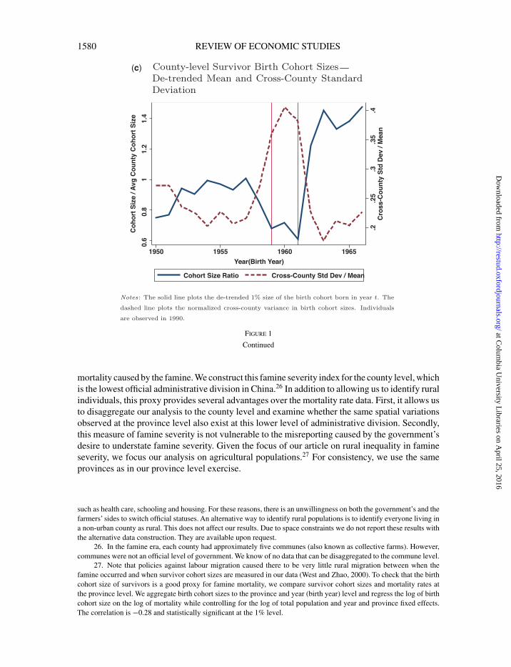
(c) —
Figure 1
Continued
mortality caused by the famine. We construct this famine severity index for the county level, whichis the lowest official administrative division in China.26 In addition to allowing us to identify ruralindividuals, this proxy provides several advantages over the mortality rate data. First, it allows usto disaggregate our analysis to the county level and examine whether the same spatial variationsobserved at the province level also exist at this lower level of administrative division. Secondly,this measure of famine severity is not vulnerable to the misreporting caused by the government’sdesire to understate famine severity. Given the focus of our article on rural inequality in famineseverity, we focus our analysis on agricultural populations.27 For consistency, we use the sameprovinces as in our province level exercise.
such as health care, schooling and housing. For these reasons, there is an unwillingness on both the government’s and thefarmers’ sides to switch official statuses. An alternative way to identify rural populations is to identify everyone living ina non-urban county as rural. This does not affect our results. Due to space constraints we do not report these results withthe alternative data construction. They are available upon request.
26. In the famine era, each county had approximately five communes (also known as collective farms). However,communes were not an official level of government. We know of no data that can be disaggregated to the commune level.
27. Note that policies against labour migration caused there to be very little rural migration between when thefamine occurred and when survivor cohort sizes are measured in our data (West and Zhao, 2000). To check that the birthcohort size of survivors is a good proxy for famine mortality, we compare survivor cohort sizes and mortality rates atthe province level. We aggregate birth cohort sizes to the province and year (birth year) level and regress the log of birthcohort size on the log of mortality while controlling for the log of total population and year and province fixed effects.The correlation is −0.28 and statistically significant at the 1% level.
at Colum
bia University L
ibraries on April 25, 2016
http://restud.oxfordjournals.org/D
ownloaded from
[17:16 23/4/2016 rdv016.tex] RESTUD: The Review of Economic Studies Page: 1581 1568–1611
MENG ET AL. INSTITUTIONAL CAUSES OF CHINA’S GREAT FAMINE 1581
The effect of famine can be observed in the birth cohort size of survivors. Figure 1bplots the size of birth cohorts in 1990 for all of China. The straight dotted line illustrates thepositive trend in birth cohort size over time, from approximately 5000 individuals per county(i.e. our sample contains 1% of the whole population) to approximately 9000 per county. Thisincrease reflects the combined forces of increased fertility and reduced infant and child mortality.The comparison of the actual birth cohort sizes and the projected linear trend shows that theformer begins to deviate from the trend for birth cohorts born as early as 1954, and sharplydeclines for individuals born during the famine (1959–1961), when the average cohort sizeis only approximately 4000 individuals. It returns to trend afterwards. The negative deviationfrom the trend suggests that individuals who were aged approximately five years and youngerwhen the famine began (i.e. those born 1954–1958) were more likely to perish than olderchildren. The steep decline for individuals born during the famine captures the additionalvulnerability of very young infants to famine and the reduction in fertility during the yearsof the famine. These patterns are consistent with the belief that adult famine victims are likelyto stop bearing children (by choice or for biological reasons) before they starve to death, as wellas qualitative accounts that very young children were more likely than adults to perish and thatvery few children were born during the famine. Note that the high survival rate of the child-bearing population is consistent with the observed rebounding of cohort sizes soon after thefamine.
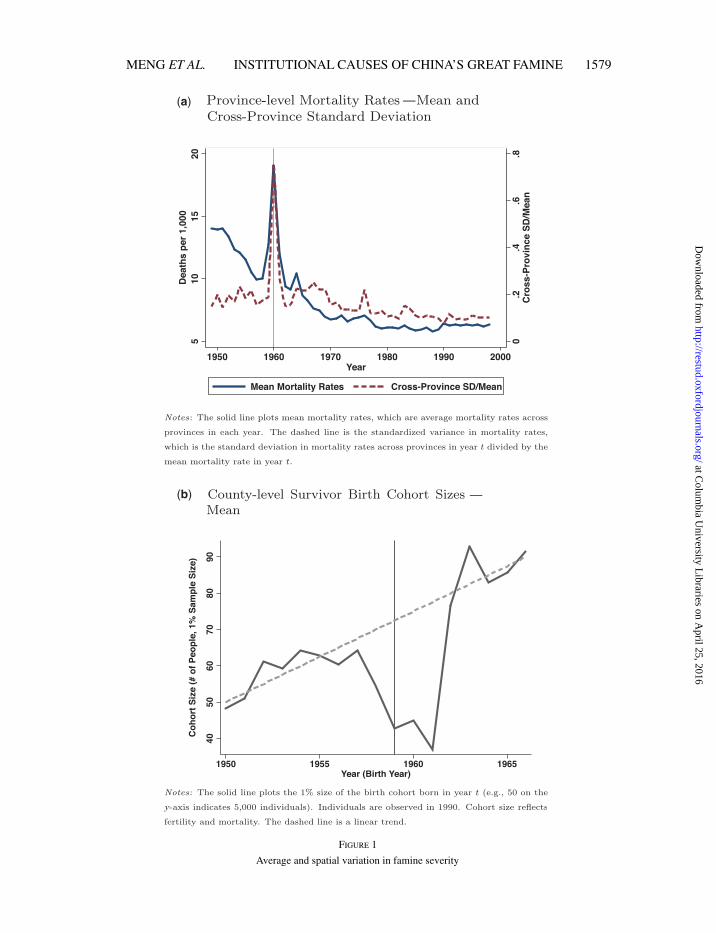
To adjust the cohort size in a way that is easily comparable to the mortality rate data shownin Figure 1, we calculate a ratio of birth cohort size in each year to the average county birthcohort size over the period 1949–1966 (because there are no data on historical county populationsizes for time of the famine), and assume that the latter is highly correlated with historical countypopulation size. As with the mortality rate data, we normalize the variance of this variable byits mean. These estimates are plotted in Figure 1c, which clearly shows a simultaneous drop incohort size and an increase in its variance for the famine years.
Using birth cohort data at the county level, we can also show that there is significant variationin famine severity across counties within provinces. See OnlineAppendix Section F and TableA.2available as Supplementary Data.
5. SPATIAL CORRELATION BETWEEN FAMINE SEVERITYAND PRODUCTIVITY
5.1. Measurement of province level productivity
In this section, we document the empirical relationship between mortality rates and agriculturalproductivity across rural areas. We find a positive correlation between mortality and productivitythat holds only during the famine years. This correlation holds both at the province level and thecounty level.
The NBS provides a measure of grain production at the province level. Our main concernwith this measure is the possibility that statisticians were unable to fully correct for governmentmisreporting of production during the GLF. In that case, the association between productivityand mortality rates during the famine would be confounded by misreporting.
To address this concern, we construct a time-varying measure of province level productionthat is unlikely to be affected by government misreporting by estimating a production functionusing data from non-GLF years (1949–1957, 1962–1982).28 To estimate the production function,
28. We restrict our attention to the years before 1982 so that our estimates can be easily comparable to the resultsin Section 6.3.2 which uses the procurement data.
at Colum
bia University L
ibraries on April 25, 2016
http://restud.oxfordjournals.org/D
ownloaded from
[17:16 23/4/2016 rdv016.tex] RESTUD: The Review of Economic Studies Page: 1582 1568–1611
1582 REVIEW OF ECONOMIC STUDIES
we regress production for province p in year t on the following production inputs: temperatureand its squared term, rainfall and its squared term, grain suitability and its squared term, ruralpopulation and its squared term, total land area and its squared term, and all combinations of thedouble interactions of temperature, rainfall, suitability, rural population, and total land area. Theproduction function regression has an adjusted R2 =0.93, which means that the input variablesexplain 93% of the variation in production.29 Then, we apply the input data from all years tocreate a measure of predicted production using the production function, which we will refer toas “constructed production” henceforth.
The only data from the GLF era that are used for the constructed production measure are theweather, total area, and population variables that are inputs in the production function. Monthlymean temperature and rainfall are reported by scientific weather stations. Access to these data wasrestricted to Chinese scientists until recently. The suitability measure is a time-invariant indexof a region’s suitability for the cultivation of the main procurement grain crops in China duringthe 1950s (rice, sorghum, wheat, buckwheat, and barley). The index is produced by the GlobalAgro-Ecological Zones (GAEZ) model developed by the Food and Agricultural Organization(FAO), and we assume the inputs are those that are similar to what was used in China during the1950s.30 The weather and suitability variables were never known to have been manipulated bythe Mao-era government. The data for total rural population and total land area are reported bythe post-Mao NBS. Since these data are difficult to manipulate and easy to correct retrospectively,their inclusion should not bias the constructed production measure.
Constructed production is similar to reported production. This can be seen in OnlineAppendixFigure A.1 available as Supplementary Data, which plots constructed grain production againstreported grain production together with the 45◦ line for each of the four years of the GLF. Thefact that constructed and reported production do not line up perfectly on the 45◦ line is consistentwith the potential presence of misreporting. However, the two measures are highly correlated forall years. To be cautious, we use the constructed measure of production for the remainder of ouranalysis. The estimates using reported production data are similar.31
We note that an earlier study, Li and Yang (2005), used additional input variables to predictproduction: the total area sown for agriculture and for grain, irrigation, the amount of agriculturemachine power, and fertilizer usage. Since these variables would have presumably been moredifficult for Chinese statisticians to correct after the famine, we did not use them as inputs toconstruct our main production measure. However, we check that our results are robust to theirinclusion.32
29. We do not report the production function coefficients because of the large number of regressors and the difficultyin interpreting each coefficient in the presence of interaction effects. They are available upon request.
30. These are based on fixed geo-climatic conditions and the technologies used by Chinese farmers in the late1950s (e.g. low level of mechanization, organic fertilizers, rain-fed irrigation). See the Online Appendix available asSupplementary Data for a detailed discussion of the weather and suitability data and the construction of province levelmeasures.
31. See Online Appendix Table A.4 available as Supplementary Data for the main results, as well as the previousversion of the article Meng et al. (2010).
32. Online Appendix Figure A.2 available as Supplementary Data plots our main constructed measure against thealternative measure, where we include these additional inputs for the famine years. The points are all close to the 45◦line in the figure. Thus, the additional inputs make little difference. We also check that the positive association betweengrain productivity and famine mortality rates is robust to using this alternative measure of grain production. The resultsare available upon request.
Like Li and Yang (2005), we predict production with inputs. However, the two studies differ conceptually inthat we use production to predict food availability and mortality, where as they use (lagged) food availability to predictinputs and do not examine mortality as a dependent variable.
at Colum
bia University L
ibraries on April 25, 2016
http://restud.oxfordjournals.org/D
ownloaded from
[17:16 23/4/2016 rdv016.tex] RESTUD: The Review of Economic Studies Page: 1583 1568–1611
MENG ET AL. INSTITUTIONAL CAUSES OF CHINA’S GREAT FAMINE 1583
5.2. Province-level analysis
With these data, we explore the relationship between food production and famine mortality rates.To provide a precise estimate of the relationship between per capita food production and mortalityrates, we pool all of the data together and estimate the following equation.
mp,t+1 =αPp,t +βPp,tIFamt +Z′
p,tγ +δt +εp,t , (1)
where mp,t+1 is the log number of deaths in province p during year t+1; Pp,t is log constructedgrain production; Pp,tIFam
t is the interaction of log constructed grain production and a dummyvariable for whether it is a famine year, where IFam
t ={0,1} is a dummy variable that equals 1 ifthe observation is of year t =1958,1959,1960; Zp,t is a vector of province–year-level covariates;δt is a vector of year fixed effects; and εp,t is an error term. The vector of covariates in the baselinespecification, Zp,t , includes the log total population, which normalizes our estimates so that wecan interpret them in “per capita” terms. We also control for the log urban population to ensure thatthe estimates capture variation driven by rural areas. Year fixed effects control for all changes overtime that affect regions similarly and they subsume the main effect for the famine year dummy.To address the presence of heteroscedasticity, all regressions estimate robust standard errors.33
Equation (1) estimates the cross-sectional correlation between productivity and mortality ratesfor non-famine years as α̂, and the correlation during the famine as ̂α+β.
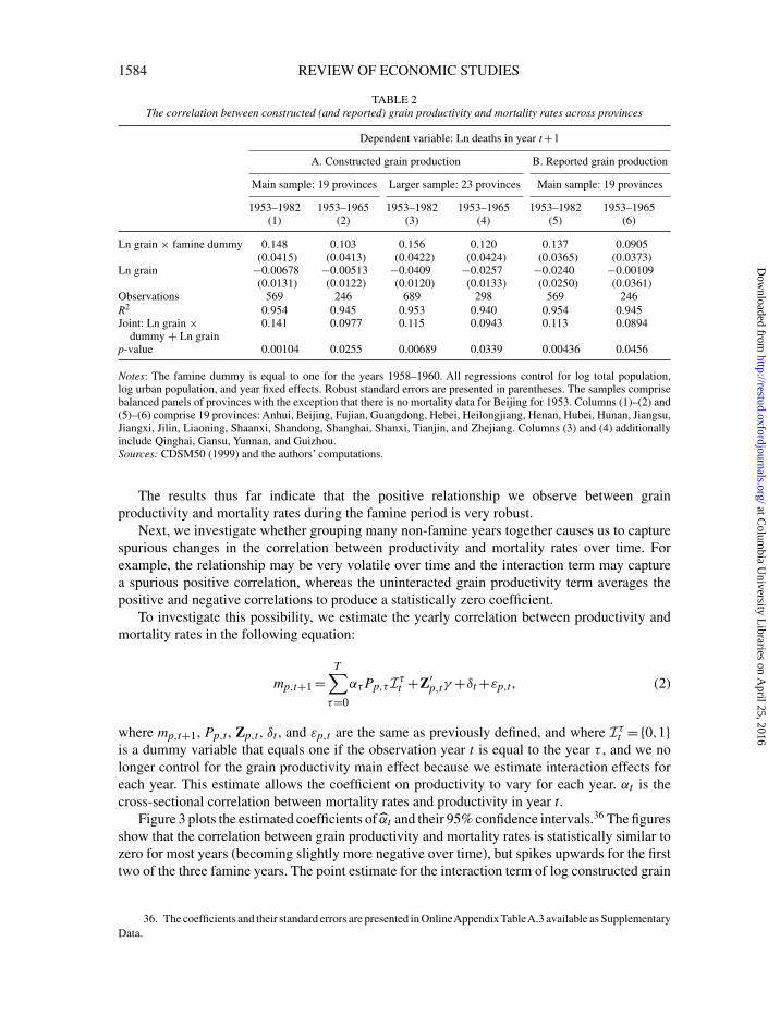
In Table 2 column (1), we show the cross-sectional correlation between productivity andmortality rates during 1953–1982.34 In column (2), we restrict the sample to five years before thefamine began until five years after the famine (1953–1965) to show that our results are driven bythe years close to the famine and not spurious correlations from long after the famine ended.35
In both columns (1) and (2), the coefficient for log constructed grain is negative and statisticallyinsignificant. This means that during normal years, higher production per capita is uncorrelatedwith mortality rates. In contrast, the interaction terms are positive and statistically significant at the1% level, which implies that the relationship between production and mortality is more positiveduring the famine years than the non-famine years. The sum of the the interaction coefficient andthe coefficient for log grain, ̂α+β, is presented at the bottom of the table along with its p-value.They are positive and statistically significant at the 1% and 5% levels.
Columns (1) and (2) use the main 19 province sample. Columns (3) and (4) use a largersample that includes the four provinces with a large proportion of ethnic minorities (OnlineAppendix Section B available as Supplementary Data). In columns (5) and (6), we present theresults using the reported historical grain production instead of our main measure of constructedgrain production and return to the main 19 province sample. The estimates are very similar. Dueto space constraints, the remainder of the article only reports results using the constructed grainproduction measures for the main sample of 19 provinces.
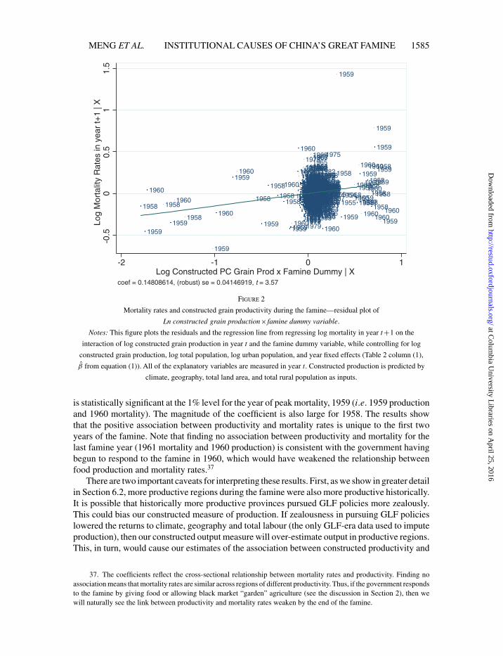
To examine whether our estimates are driven by outliers, we plot the residuals of the regressionsin column (1) of Table 2. Figure 2 plots the residuals for the interaction of log constructed grainand the dummy variable for the three famine years. As seen in the regression, the relationship ispositive and not driven by outliers.
33. Our results are similar if we estimate wild bootstrapped standard errors that are clustered at the province leveland adjust for the small number of clusters (Cameron et al. 2008). These results are not presented due to space restrictions.The robustness of our estimates to different levels of clustering can also be seen later, when we present the county levelanalysis that cluster standard errors at the province level.
34. Before 1953, mortality data were not available for all provinces.35. The estimates are similar if we use a sample with a longer time horizon (e.g. until 1998).
at Colum
bia University L
ibraries on April 25, 2016
http://restud.oxfordjournals.org/D
ownloaded from
[17:16 23/4/2016 rdv016.tex] RESTUD: The Review of Economic Studies Page: 1584 1568–1611
1584 REVIEW OF ECONOMIC STUDIES
TABLE 2The correlation between constructed (and reported) grain productivity and mortality rates across provinces
Dependent variable: Ln deaths in year t+1
A. Constructed grain production B. Reported grain production
Main sample: 19 provinces Larger sample: 23 provinces Main sample: 19 provinces
1953–1982 1953–1965 1953–1982 1953–1965 1953–1982 1953–1965(1) (2) (3) (4) (5) (6)
Ln grain × famine dummy 0.148 0.103 0.156 0.120 0.137 0.0905(0.0415) (0.0413) (0.0422) (0.0424) (0.0365) (0.0373)
Ln grain −0.00678 −0.00513 −0.0409 −0.0257 −0.0240 −0.00109(0.0131) (0.0122) (0.0120) (0.0133) (0.0250) (0.0361)
Observations 569 246 689 298 569 246R2 0.954 0.945 0.953 0.940 0.954 0.945Joint: Ln grain × 0.141 0.0977 0.115 0.0943 0.113 0.0894
dummy + Ln grainp-value 0.00104 0.0255 0.00689 0.0339 0.00436 0.0456
Notes: The famine dummy is equal to one for the years 1958–1960. All regressions control for log total population,log urban population, and year fixed effects. Robust standard errors are presented in parentheses. The samples comprisebalanced panels of provinces with the exception that there is no mortality data for Beijing for 1953. Columns (1)–(2) and(5)–(6) comprise 19 provinces: Anhui, Beijing, Fujian, Guangdong, Hebei, Heilongjiang, Henan, Hubei, Hunan, Jiangsu,Jiangxi, Jilin, Liaoning, Shaanxi, Shandong, Shanghai, Shanxi, Tianjin, and Zhejiang. Columns (3) and (4) additionallyinclude Qinghai, Gansu, Yunnan, and Guizhou.Sources: CDSM50 (1999) and the authors’ computations.
The results thus far indicate that the positive relationship we observe between grainproductivity and mortality rates during the famine period is very robust.
Next, we investigate whether grouping many non-famine years together causes us to capturespurious changes in the correlation between productivity and mortality rates over time. Forexample, the relationship may be very volatile over time and the interaction term may capturea spurious positive correlation, whereas the uninteracted grain productivity term averages thepositive and negative correlations to produce a statistically zero coefficient.
To investigate this possibility, we estimate the yearly correlation between productivity andmortality rates in the following equation:
mp,t+1 =T∑
τ=0
ατ Pp,τIτt +Z′
p,tγ +δt +εp,t , (2)
where mp,t+1, Pp,t , Zp,t , δt , and εp,t are the same as previously defined, and where Iτt ={0,1}
is a dummy variable that equals one if the observation year t is equal to the year τ , and we nolonger control for the grain productivity main effect because we estimate interaction effects foreach year. This estimate allows the coefficient on productivity to vary for each year. αt is thecross-sectional correlation between mortality rates and productivity in year t.
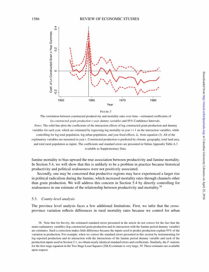
Figure 3 plots the estimated coefficients of α̂t and their 95% confidence intervals.36 The figuresshow that the correlation between grain productivity and mortality rates is statistically similar tozero for most years (becoming slightly more negative over time), but spikes upwards for the firsttwo of the three famine years. The point estimate for the interaction term of log constructed grain
36. The coefficients and their standard errors are presented in OnlineAppendix TableA.3 available as SupplementaryData.
at Colum
bia University L
ibraries on April 25, 2016
http://restud.oxfordjournals.org/D
ownloaded from
[17:16 23/4/2016 rdv016.tex] RESTUD: The Review of Economic Studies Page: 1585 1568–1611
MENG ET AL. INSTITUTIONAL CAUSES OF CHINA’S GREAT FAMINE 1585
1958
1959
1960
1958
1959
1960
1958
1959
1960
19591960
1958
1959
1958
1958
1960
1958
195919591960
1960
1979
19541955
1960
195519571956
1954
1954
1955
1956
1982
197619571975197119771981198119741972198019781969
19531979
1956198019661967
1962
197319821978
195719691976
19651953
1968
197419771979
19641963197019731974197319681971
1964
1975
19671961
197219721971196319761982196619651980198119751978197719621954
1959
1961197919701967196619531962
1954
1955
1956
1961
196519541969195519561955
19641969196819571978
1965196219641974
1957
197019751982
19631966
19551973198019811972197619711968
19571961198019821956
196719541981
1955
1963
1974
19771953
1973
19751972197919761971
1957
1978
1956
1977
19701967
1953
197019611955
1957195419621961
19651968
1962
1954
19741966
19541970
19771971
1953
19811969
198119641963
1956
1980
1982
1972
1973
19641976
1975
1974
1964
197819761977
1970
19751978196319621973
1955
1961
1969
1965
1965
1966
19631968
19691972
1982
1979
1982
1979
1980
1981
1967
1971
1966
1968
1956
1980
1957
1967197419761978
1953
1957
19751977
195619721973
1979
1967196819701966196519701962
19711962
1961
19631961
197119701969
19731981
1953
1963196919651968
1972196419661967
19641980197519781968
19741953
198219721971
1979
1973198019761977197819751966197419761967
196819771982
19751976196919771964
1974197819801970
1981
1963
1969197119721966
196219651961
19731982197919671965
19791981
1963
1953
19611958196419621957
19821978197719761974198019551954
1979
195619731970197219811971
1954
196919751967
195519611964195619651963
19531957196819661962
1955
1953
1954
1973
1963
1974
197519781957196819771956
19721976198019811955
1955
1967
1975
1965
197019781971198119701969197719731962
1966
1954
1971
1968
1974
19821979
1964
1979
1961
1980198219691954197219621976
1963
19561964
1953
1967
19651972
1960
1981
1966
198219771957
19771980
1961197319751976
1970
19781961197419791966
197619821981
1964
19701968
1971
1979195619801956197819751974
1965
1968
1971
1969
19571969
19531963
196719671953196619731972
1963
19551957
1962
1962196419541965
1961
19621961
1963195319641965
195919661967196819691970195419711972
1955
19731975
1957
197619771978198019811982
1956
1979
1953
197419631964196219651961
1966
1967
1968
195419691955
1970
196319621964
19571971195619741972196519731975
1961
1977
1960
1978197619821981
1966
1980
1967196819791969
19531970197119721974
1975
1973197719761978
1982198119801979
19571956
1958
1959
19551954
1959
19581960
19601958
19591958
1960
1959
1959
1958
1960
195819601960
1960
1958
1958
1958
1959
1960
1958
1959
1958
1959
1959
1959
1960
-0.5
00.
51
1.5
Log
Mor
talit
y R
ates
in y
ear
t+1
| X
-2 -1 0 1Log Constructed PC Grain Prod x Famine Dummy | X
coef = 0.14808614, (robust) se = 0.04146919, t = 3.57
Figure 2
Mortality rates and constructed grain productivity during the famine—residual plot of
Ln constructed grain production×famine dummy variable.
Notes: This figure plots the residuals and the regression line from regressing log mortality in year t+1 on the
interaction of log constructed grain production in year t and the famine dummy variable, while controlling for log
constructed grain production, log total population, log urban population, and year fixed effects (Table 2 column (1),
β̂ from equation (1)). All of the explanatory variables are measured in year t. Constructed production is predicted by
climate, geography, total land area, and total rural population as inputs.
is statistically significant at the 1% level for the year of peak mortality, 1959 (i.e. 1959 productionand 1960 mortality). The magnitude of the coefficient is also large for 1958. The results showthat the positive association between productivity and mortality rates is unique to the first twoyears of the famine. Note that finding no association between productivity and mortality for thelast famine year (1961 mortality and 1960 production) is consistent with the government havingbegun to respond to the famine in 1960, which would have weakened the relationship betweenfood production and mortality rates.37
There are two important caveats for interpreting these results. First, as we show in greater detailin Section 6.2, more productive regions during the famine were also more productive historically.It is possible that historically more productive provinces pursued GLF policies more zealously.This could bias our constructed measure of production. If zealousness in pursuing GLF policieslowered the returns to climate, geography and total labour (the only GLF-era data used to imputeproduction), then our constructed output measure will over-estimate output in productive regions.This, in turn, would cause our estimates of the association between constructed productivity and
37. The coefficients reflect the cross-sectional relationship between mortality rates and productivity. Finding noassociation means that mortality rates are similar across regions of different productivity. Thus, if the government respondsto the famine by giving food or allowing black market “garden” agriculture (see the discussion in Section 2), then wewill naturally see the link between productivity and mortality rates weaken by the end of the famine.
at Colum
bia University L
ibraries on April 25, 2016
http://restud.oxfordjournals.org/D
ownloaded from
[17:16 23/4/2016 rdv016.tex] RESTUD: The Review of Economic Studies Page: 1586 1568–1611
1586 REVIEW OF ECONOMIC STUDIES
-0.2
00.
20.
4
Coe
f. of
Ln
Con
stru
cted
Gra
in x
Yea
r D
umm
ies
1950 1960 1970 1980
Year
Figure 3
The correlation between constructed productivity and mortality rates over time—estimated coefficients of
Ln constructed grain production×year dummy variables and 95% Confidence Intervals.
Notes: The solid line plots the coefficients of the interaction effects of log constructed grain production and dummy
variables for each year, which are estimated by regressing log mortality in year t+1 on the interaction variables, while
controlling for log total population, log urban population, and year fixed effects. α̂τ from equation (2). All of the
explanatory variables are measured in year t. Constructed production is predicted by climate, geography, total land area,
and total rural population as inputs. The coefficients and standard errors are presented in Online Appendix Table A.3
available as Supplementary Data.
famine mortality to bias upward the true association between productivity and famine mortality.In Section 5.4, we will show that this is unlikely to be a problem in practice because historicalproductivity and political zealousness were not positively associated.
Secondly, one may be concerned that productive regions may have experienced a larger risein political radicalism during the famine, which increased mortality rates through channels otherthan grain production. We will address this concern in Section 5.4 by directly controlling forzealousness in our estimate of the relationship between productivity and mortality.38
5.3. County-level analysis
The province level analysis faces a few additional limitations. First, we infer that the cross-province variation reflects differences in rural mortality rates because we control for urban
38. Note that for brevity, the estimated standard errors presented in the article do not correct for the fact that themain explanatory variables (log constructed grain production and its interaction with the famine period dummy variable)are estimates. Such a correction makes little difference because the inputs used to predict production explain 93% of thevariation in production. For example, when we correct the standard errors presented in this section by instrumenting forlog reported production and its interaction with the interactions of the famine period dummy variable and each of theproduction inputs used in Section 5.1, we obtain nearly identical standard errors and coefficients. Similarly, the F-statisticfor the first stage equation in the Two Stage Least Squares (2SLS) estimate is very large, 39. These estimates are availableupon request.
at Colum
bia University L
ibraries on April 25, 2016
http://restud.oxfordjournals.org/D
ownloaded from
[17:16 23/4/2016 rdv016.tex] RESTUD: The Review of Economic Studies Page: 1587 1568–1611
MENG ET AL. INSTITUTIONAL CAUSES OF CHINA’S GREAT FAMINE 1587
population, but the mortality data do not explicitly distinguish between urban and rural areas.Secondly, the official mortality data, like the official production data, may be measured with error.Finally, there may be variation across rural areas within a province that we cannot observe withthe province level analysis.
We address these concerns by using county level data that include only agriculturalpopulations. This allows us to check that there is variation across rural areas and control forprovince fixed effects to examine whether there is variation within provinces as well as acrossprovinces. This exercise also proxies for famine severity using data that was not potentiallymanipulated by the Chinese government to check that positive association between famineseverity and food productivity at the province level are not driven by government misreporting.
The main dependent variable is the alternative proxy for famine severity—birth cohort size,which is the size of each birth cohort observed in the 1% sample of the 1990 China PopulationCensus. The main drawback of using birth cohort size to proxy for famine severity is that it cannotcapture the mortality rates of the elderly, who are also believed to have suffered high faminemortality rates. Another related issue is that while it is reasonable to assume that famine mortalityis negatively correlated with survivor birth cohort size, we do not know the functional form of thisrelationship. Thus, we can only use the relationship between birth cohort size and productivityto test the robustness of the sign of the relationship between mortality and productivity.
The explanatory variables are measures of annual (time-varying) mean spring temperature,rainfall, and a (time-invariant) measure of the suitability for grain cultivation, which are thedisaggregated measures of the variables used in the province level production function inSection 5.1. We examine these directly (rather than a constructed production measure from theproduction function) to check that the earlier results are indeed driven by natural conditions. Inthis exercise, we interpret the measures of natural conditions as proxies of productivity.
For consistency, we restrict the sample to the same 19 provinces used in the province levelmortality rate analysis. The limited number of historical weather stations additionally restrictsthe final sample, which includes 511 counties. Our sample begins with 1950, the first year forwhich there is disaggregated weather data, and ends before 1966 to avoid potentially confoundingeffects of post-famine political events on fertility.39
We examine the relationship between survivor cohort size and proxies for agriculturalproductivity across rural counties. If the interpretation of our main results are correct, thenwe should find similar patterns over time between natural conditions that are advantageous forproduction and survivor birth cohort size—that is good conditions should have no relationship ora positive relationship with birth cohort size for cohorts not affected by the famine, but a negativerelationship for cohorts affected by the famine. Due to space restrictions, we focus on the year-by-year estimates using equation (2). This differs from earlier estimates in that observations arenow at the county and year level, and we control for log average birth cohort size to normalize bythe population. We also control for province fixed effects to examine whether the same patternsexist within provinces as across provinces. In our regression, we simultaneously include theinteractions of year dummy variables with each of the three proxies of productivity: mean logspring temperature, mean log spring rainfall, and the suitability for grain cultivation index. Thestandard errors are clustered at the county level. The coefficients and standard errors are reportedin Online Appendix Table A.6 available as Supplementary Data.
39. See the OnlineAppendix available as Supplementary Data for a detailed description of the weather and suitabilitydata. We exclude the post-1966 period because the Cultural Revolution (1966–1976) caused political disruptions thatmay have delayed fertility. This is less of an issue for the province level mortality estimates because this revolution wasnot associated with abnormal mortality rates. The results are similar if we extend the panel to include those born duringor after 1966. They are not reported due to space constraints, but are available upon request.
at Colum
bia University L
ibraries on April 25, 2016
http://restud.oxfordjournals.org/D
ownloaded from
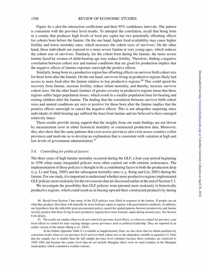
[17:16 23/4/2016 rdv016.tex] RESTUD: The Review of Economic Studies Page: 1588 1568–1611
1588 REVIEW OF ECONOMIC STUDIES
Figure 4a–c plot the interaction coefficients and their 95% confidence intervals. The patternis consistent with the province level results. To interpret the correlation, recall that being bornin a county that produces high levels of food per capita has two potentially offsetting effectsfor cohorts born before the famine. On the one hand, higher food availability may cause higherfertility and lower mortality rates, which increases the cohort sizes of survivors. On the otherhand, these individuals are exposed to a more severe famine at very young ages, which reducesthe cohort size of survivors. Similarly, for the cohort born during the famine, the more severefamine faced by women of child-bearing age may reduce fertility. Therefore, finding a negativecorrelation between cohort size and natural conditions that are good for production implies thatthe negative effects of famine exposure outweigh the positive effects.
Similarly, being born in a productive region has offsetting effects on survivor birth cohort sizefor those born after the famine. On the one hand, survivors living in productive regions likely hadaccess to more food after the famine relative to less productive regions.40 This could speed therecovery from famine, increase fertility, reduce infant mortality, and thereby, increase survivorcohort sizes. On the other hand, famines of greater severity in productive regions mean that theseregions suffer larger population losses, which result in a smaller population base for bearing andrearing children after the famine. The finding that the correlation between survivor birth cohortsizes and natural conditions are zero or positive for those born after the famine implies that thepositive effects outweigh or cancel the negative effects. This is not altogether surprising sinceindividuals of child-bearing age suffered the least from famine and are believed to have emergedrelatively intact.
These results provide strong support that the insights from our main findings are not drivenby measurement error in either historical mortality or constructed production data. Moreover,they also show that the same patterns that exist across provinces also exist across counties withinprovinces and motivate us to develop an explanation that is consistent with variation at high andlow levels of government administration.41
5.4. Controlling for political factors
The three years of high famine mortality occurred during the GLF, a four-year period beginningin 1958 when many misguided policies were often carried out with extreme zealousness. Theimplementation of these policies is thought to be a contributing factor to both the production drop(e.g. Li and Yang, 2005) and the subsequent mortality rates (e.g. Kung and Lin, 2003) during thefamine. For our study, it is important to understand whether more productive regions implementedGLF policies more zealously for the two reasons that are discussed earlier at the end of Section 5.2.
We investigate the possibility that GLF policies were pursued more zealously in historicallyproductive regions, which could result us in biasing upward their constructed productivity during
40. Recall from Section 2 that many of the GLF policies were lifted in response to the famine. If people can eatwhat they produce, then there will naturally be more food per capita in regions with good natural conditions. In addition,our hypothesis that the inflexible grain procurement policy caused the spatial patterns between productivity and famineseverity predicts that those living in more productive regions have more food per capita during normal years. See Section6 for details.
41. The results are similar when we do not control for province fixed effects, or when we control for province–yearfixed effects to control for time-varying changes across provinces such as political leadership. They are reported in anearlier version of the article (Meng et al., 2010).
In the Online Appendix Table A.5 available as Supplementary Data, we also show that we obtain qualitativelyconsistent results when we use province level survivor birth cohort size as the dependent variable in equation (1). Notethat the sample size is smaller than the full sample province level estimates because these estimates are restricted to1950–1965 and because the county level data do not include Shanghai (there were no rural counties in the Shanghaimunicipality which contained a weather station).
at Colum
bia University L
ibraries on April 25, 2016
http://restud.oxfordjournals.org/D
ownloaded from
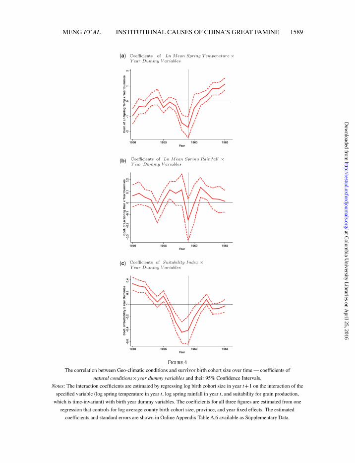
[17:16 23/4/2016 rdv016.tex] RESTUD: The Review of Economic Studies Page: 1589 1568–1611
MENG ET AL. INSTITUTIONAL CAUSES OF CHINA’S GREAT FAMINE 1589
(a)
(b)
(c)
Figure 4
The correlation between Geo-climatic conditions and survivor birth cohort size over time — coefficients of
natural conditions×year dummy variables and their 95% Confidence Intervals.
Notes: The interaction coefficients are estimated by regressing log birth cohort size in year t+1 on the interaction of the
specified variable (log spring temperature in year t, log spring rainfall in year t, and suitability for grain production,
which is time-invariant) with birth year dummy variables. The coefficients for all three figures are estimated from one
regression that controls for log average county birth cohort size, province, and year fixed effects. The estimated
coefficients and standard errors are shown in Online Appendix Table A.6 available as Supplementary Data.
at Colum
bia University L
ibraries on April 25, 2016
http://restud.oxfordjournals.org/D
ownloaded from
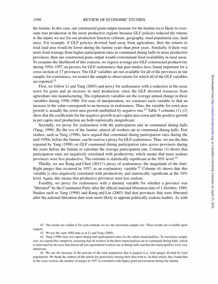
[17:16 23/4/2016 rdv016.tex] RESTUD: The Review of Economic Studies Page: 1590 1568–1611
1590 REVIEW OF ECONOMIC STUDIES
the famine. In this case, our constructed grain output measure for the famine era is likely to over-state true production in the more productive regions because GLF policies reduced the returnsto the inputs we use for our production function (climate, geography, rural population size, landarea). For example, if GLF policies diverted land away from agriculture, then the returns tototal land area would be lower during the famine years than prior years. Similarly, if there wasmore food wastage from higher participation rates in communal dining halls in more productiveprovinces, then our constructed grain output would overestimate food availability in rural areas.To examine the likelihood of this concern, we regress average pre-GLF constructed productivityduring 1954–1957 on proxies for GLF zealousness that past studies have found important for across-section of 17 provinces. The GLF variables are not available for all of the provinces in oursample; for consistency, we restrict the sample to observations for which all of the GLF variablesare reported.42
First, we follow Li and Yang (2005) and proxy for zealousness with a reduction in the areassown for grain and an increase in steel production, since the GLF diverted resources fromagriculture into manufacturing. The explanatory variables are the average annual change in thesevariables during 1958–1960. For ease of interpretation, we construct each variable so that anincrease in the value corresponds to an increase in zealousness. Thus, the variable for sown areagrowth is actually the sown area growth multiplied by negative one.43 Table 3 columns (1)–(2)show that the coefficients for the negative growth in per capita area sown and the positive growthin per capita steel production are both statistically insignificant.
Secondly, we proxy for zealousness with the participation rate in communal dining halls(Yang, 1998). By the eve of the famine, almost all workers ate in communal dining halls. Paststudies, such as Yang (1998), have argued that communal dining participation rates during themid-1950s, before the famine, can be used as a proxy for GLF zealousness. Thus, we use the datareported by Yang (1998) on GLF communal dining participation rates across provinces duringthe years before the famine to calculate the average participation rate. Column (3) shows thatparticipation rates are negatively correlated with productivity, which means that more zealousprovinces were less productive. The estimate is statistically significant at the 10% level.44
Thirdly, we use Kung and Chen (2011)’s proxy of zealousness, the magnitude of the Anti-Right purges that occurred in 1957, as an explanatory variable.45 Column (4) shows that thisvariable is also negatively correlated with productivity and statistically significant at the 10%level. Again, this means that productive provinces were less zealous.
Fourthly, we proxy for zealousness with a dummy variable for whether a province was“liberated” by the Communist Party after the official national liberation date of 1 October, 1949.Studies such as Yang (1998) and Kung and Lin (2003) find that provinces that were liberatedafter the national liberation date were more likely to appoint politically zealous leaders. As with
42. Our results are similar if for each estimate we use the maximum sample size. These results are available uponrequest.
43. We use the same NBS data as in Li and Yang (2005).44. Yang (1998) does not report dining hall participation rates for the urban municipalities. To maximize sample
size, we expand this sample by assuming that all workers in the three municipalities ate in communal dining halls, whichis motivated by the facts that almost all non-agricultural workers ate in dining halls and that the municipalities were veryurbanized.
45. We use the measure of the percent of the total population that is purged (e.g. total purges divided by totalpopulation). We thank the authors of this article for generously sharing their data with us. In their article, they found thatin the cross-section, the number of purges in 1957 is correlated with higher grain procurement during the famine.
at Colum
bia University L
ibraries on April 25, 2016
http://restud.oxfordjournals.org/D
ownloaded from
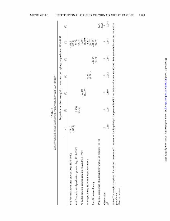
[17:16 23/4/2016 rdv016.tex] RESTUD: The Review of Economic Studies Page: 1591 1568–1611
MENG ET AL. INSTITUTIONAL CAUSES OF CHINA’S GREAT FAMINE 1591
TAB
LE
3T
heco
rrel
atio
nbe
twee
nco
nstr
ucte
dgr
ain
prod
ucti
vity
and
GL
Fin
tens
ity
Dep
ende
ntva
riab
le:a
vera
geL
nco
nstr
ucte
dpe
rca
pita
grai
npr
oduc
tion
1954
–195
7
(1)
(2)
(3)
(4)
(5)
(6)
(7)
(−)
Per
capi
taso
wn
area
grow
th(A
vg.1
958–
1960
)−7
54.0
−291
.3(5
32.9
)(8
62.9
)(+
)Pe
rca
pita
stee
lpro
duct
ion
grow
th(A
vg.1
958–
1960
)8.
430
20.6
6(5
8.84
)(6
6.87
)%
Part
icip
atio
nin
com
mun
aldi
ning
(Avg
.195
5–19
58)
−2.0
00−0
.694
(1.0
79)
(1.4
80)
%Pu
rged
duri
ng19
57A
nti-
Rig
htM
ovem
ent
−16.
34−8
.813
(8.3
81)
(14.
65)
Lat
elib
erat
ion
dum
my
−94.
45−8
1.92
(59.
36)
(77.
39)
Prin
cipa
lcom
pone
ntof
inde
pend
entv
aria
bles
inco
lum
ns(1
)–(6
)−4
2.47
(19.
28)
Obs
erva
tions
1717
1717
1717
17R
20.
118
0.00
10.
186
0.20
20.
144
0.34
80.
244
Not
es:
The
sam
ple
com
pris
es17
prov
ince
s.In
colu
mn
(7),
we
cont
rolf
orth
epr
inci
palc
ompo
nent
the
GL
Fva
riab
les
used
inco
lum
ns(1
)–(6
).R
obus
tsta
ndar
der
rors
are
repo
rted
inpa
rent
hese
s.So
urce
s:se
ete
xt.
at Colum
bia University L
ibraries on April 25, 2016
http://restud.oxfordjournals.org/D
ownloaded from
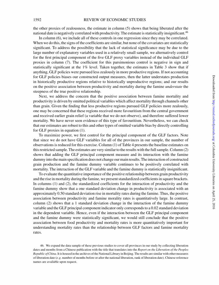
[17:16 23/4/2016 rdv016.tex] RESTUD: The Review of Economic Studies Page: 1592 1568–1611
1592 REVIEW OF ECONOMIC STUDIES
the other proxies of zealousness, the estimate in column (5) shows that being liberated after thenational date is negatively correlated with productivity. The estimate is statistically insignificant.46
In column (6), we include all of these controls in one regression since they may be correlated.When we do this, the signs of the coefficients are similar, but none of the covariates are statisticallysignificant. To address the possibility that the lack of statistical significance may be due to thelarge number of explanatory variables used in a relatively small sample, we alternatively controlfor the first principal component of the five GLF proxy variables instead of the individual GLFproxies in column (7). The coefficient for this parsimonious control is negative in sign andstatistically significant at the 1% level. Taken together, the estimates in Table 3 show that ifanything, GLF policies were pursued less zealously in more productive regions. If not accountingfor GLF policies biases our constructed output measures, then the latter understates productionin historically productive regions relative to historically unproductive regions; and our resultson the positive association between productivity and mortality during the famine understate thesteepness of the true positive relationship.
Next, we address the concern that the positive association between famine mortality andproductivity is driven by omitted political variables which affect mortality through channels otherthan grain. Given the finding that less productive regions pursued GLF policies more zealously,one may be concerned that these regions received more favouritism from the central governmentand received earlier grain relief (a variable that we do not observe), and therefore suffered lowermortality. We have never seen evidence of this type of favouritism. Nevertheless, we can checkthat our estimates are robust to this and other types of omitted variable bias by directly controllingfor GLF proxies in equation (1).
To maximize power, we first control for the principal component of the GLF factors. Notethat since we do not have GLF variables for all of the provinces in our sample, the number ofobservations is reduced for this exercise. Column (1) of Table 4 presents the baseline estimates onthis restricted sample. The estimates are very similar to the results with the full sample. Column (2)shows that adding the GLF principal component measure and its interaction with the faminedummy into the main specification does not change our main results. The interaction of constructedgrain production and the famine dummy variable continues to be positively correlated withmortality. The interaction of the GLF variable and the famine dummy is statistically insignificant.
To evaluate the quantitative importance of the positive relationship between grain productivityand the rise in mortality during the famine, we present standardized coefficients in square brackets.In columns (1) and (2), the standardized coefficients for the interaction of productivity and thefamine dummy show that a one standard deviation change in productivity is associated with anapproximately 0.50 standard deviation rise in mortality rates during the famine. Thus, the positiveassociation between productivity and famine morality rates is quantitatively large. In contrast,column (2) shows that a 1 standard deviation change in the interaction of the famine dummyvariable and the GLF principal component indicator only corresponds to a 0.02 standard deviationin the dependent variable. Hence, even if the interaction between the GLF principal componentand the famine dummy were statistically significant, we would still conclude that the positiveassociation between food productivity and mortality rates is more quantitatively important forunderstanding mortality rates than the relationship between GLF factors and famine mortalityrates.
46. We expand the data sample of these previous studies to cover all provinces in our study by collecting liberationdates and months from a Chinese publication with the title that translates into the Report on the Liberation of the PeoplesRepublic of China. It is housed in the archives of the National Library in Beijing. The results are similar with other measuresof liberation date (e.g. number of months before or after the national liberation, rank of liberation date). Chinese referencenames are available upon request.
at Colum
bia University L
ibraries on April 25, 2016
http://restud.oxfordjournals.org/D
ownloaded from
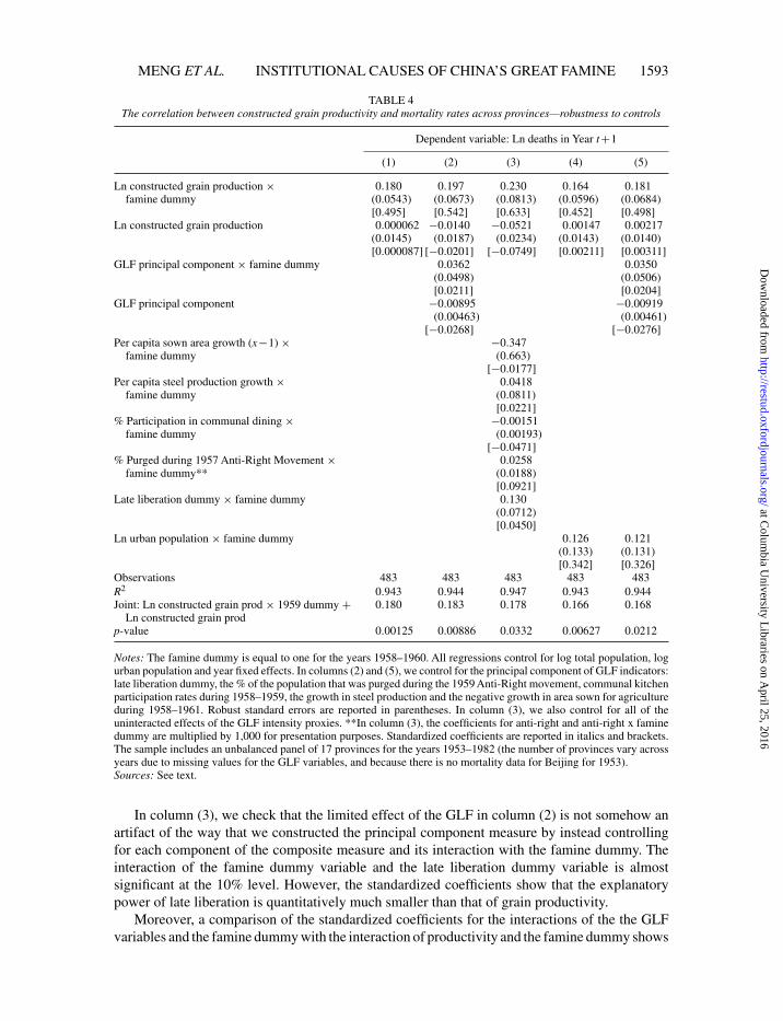
[17:16 23/4/2016 rdv016.tex] RESTUD: The Review of Economic Studies Page: 1593 1568–1611
MENG ET AL. INSTITUTIONAL CAUSES OF CHINA’S GREAT FAMINE 1593
TABLE 4The correlation between constructed grain productivity and mortality rates across provinces—robustness to controls
Dependent variable: Ln deaths in Year t+1
(1) (2) (3) (4) (5)
Ln constructed grain production × 0.180 0.197 0.230 0.164 0.181famine dummy (0.0543) (0.0673) (0.0813) (0.0596) (0.0684)
[0.495] [0.542] [0.633] [0.452] [0.498]Ln constructed grain production 0.000062 −0.0140 −0.0521 0.00147 0.00217
(0.0145) (0.0187) (0.0234) (0.0143) (0.0140)[0.000087] [−0.0201] [−0.0749] [0.00211] [0.00311]
GLF principal component × famine dummy 0.0362 0.0350(0.0498) (0.0506)[0.0211] [0.0204]
GLF principal component −0.00895 −0.00919(0.00463) (0.00461)
[−0.0268] [−0.0276]Per capita sown area growth (x−1) × −0.347
famine dummy (0.663)[−0.0177]
Per capita steel production growth × 0.0418famine dummy (0.0811)
[0.0221]% Participation in communal dining × −0.00151
famine dummy (0.00193)[−0.0471]
% Purged during 1957 Anti-Right Movement × 0.0258famine dummy** (0.0188)
[0.0921]Late liberation dummy × famine dummy 0.130
(0.0712)[0.0450]
Ln urban population × famine dummy 0.126 0.121(0.133) (0.131)[0.342] [0.326]
Observations 483 483 483 483 483R2 0.943 0.944 0.947 0.943 0.944Joint: Ln constructed grain prod × 1959 dummy + 0.180 0.183 0.178 0.166 0.168
Ln constructed grain prodp-value 0.00125 0.00886 0.0332 0.00627 0.0212
Notes: The famine dummy is equal to one for the years 1958–1960. All regressions control for log total population, logurban population and year fixed effects. In columns (2) and (5), we control for the principal component of GLF indicators:late liberation dummy, the % of the population that was purged during the 1959 Anti-Right movement, communal kitchenparticipation rates during 1958–1959, the growth in steel production and the negative growth in area sown for agricultureduring 1958–1961. Robust standard errors are reported in parentheses. In column (3), we also control for all of theuninteracted effects of the GLF intensity proxies. **In column (3), the coefficients for anti-right and anti-right x faminedummy are multiplied by 1,000 for presentation purposes. Standardized coefficients are reported in italics and brackets.The sample includes an unbalanced panel of 17 provinces for the years 1953–1982 (the number of provinces vary acrossyears due to missing values for the GLF variables, and because there is no mortality data for Beijing for 1953).Sources: See text.
In column (3), we check that the limited effect of the GLF in column (2) is not somehow anartifact of the way that we constructed the principal component measure by instead controllingfor each component of the composite measure and its interaction with the famine dummy. Theinteraction of the famine dummy variable and the late liberation dummy variable is almostsignificant at the 10% level. However, the standardized coefficients show that the explanatorypower of late liberation is quantitatively much smaller than that of grain productivity.
Moreover, a comparison of the standardized coefficients for the interactions of the the GLFvariables and the famine dummy with the interaction of productivity and the famine dummy shows
at Colum
bia University L
ibraries on April 25, 2016
http://restud.oxfordjournals.org/D
ownloaded from
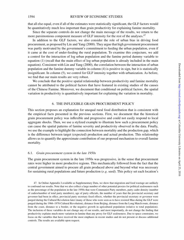
[17:16 23/4/2016 rdv016.tex] RESTUD: The Review of Economic Studies Page: 1594 1568–1611
1594 REVIEW OF ECONOMIC STUDIES
that all else equal, even if all of the estimates were statistically significant, the GLF factors wouldbe quantitatively much less important than grain productivity for explaining famine mortality.
Since the separate controls do not change the main message of the results, we return to themore parsimonious component measure of GLF intensity for the rest of the analyses.47
In addition to the GLF factors, we also consider the role of urban bias in driving foodprocurement, as proposed by Lin and Yang (2000). They argue that high government procurementwas partly motivated by the government’s commitment to feeding the urban population, even ifit came at the cost of under-feeding the rural population. To examine this conjecture, we adda control for the interaction of log urban population and the famine period dummy variable toequation (1) (recall that the main effect of log urban population is already included in the mainequation). Consistent with Lin and Yang (2000), the correlation between the interaction of urbanpopulation and the famine dummy variable in column (4) is positive in sign, but it is statisticallyinsignificant. In column (5), we control for GLF intensity together with urbanization. As before,we find that our main results are very robust.
We conclude that the positive spatial relationship between productivity and famine mortalitycannot be attributed to the political factors that have featured in existing studies of the causesof the Chinese Famine. Moreover, we document that conditional on political factors, the spatialvariation in productivity is quantitatively important for explaining the variation in mortality.
6. THE INFLEXIBLE GRAIN PROCUREMENT POLICY
This section proposes an explanation for unequal rural food distribution that is consistent withthe empirical facts presented in the previous sections. First, we document that the historicalgrain procurement policy was inflexible and progressive and could not easily respond to localaggregate shocks. Then, we use a stylized example to illustrate how such a procurement policycan cause the spatial patterns of famine severity and productivity observed in the data. Finally,we use the example to highlight the connection between mortality and the production gap, whichis the difference between target (expected) production and actual production. This relationshipallows us to quantify the approximate contribution of our proposed mechanism to overall faminemortality.
6.1. Grain procurement system in the late 1950s
The grain procurement system in the late 1950s was progressive, in the sense that procurementrates were higher in more productive regions. This mechanically followed from the fact that thecentral government aimed to procure all grain produced above and beyond what was necessaryfor sustaining rural populations and future production (e.g. seed). This policy set each location’s
47. In Online Appendix I available as Supplementary Data, we show that migration and food wastage are unlikelyto confound our results. Note that we also collect a large number of other potential proxies for political zealousness suchas the percentage of the population in the late 1950s that were Communist Party members, party cadre density (numberof cadres/number of total party members), age of party officials, the number of years that the provincial secretary andgovernor had been in office, provincial party secretary fixed effects, whether the provincial secretary or governor werepurged during the Cultural Revolution later (many of those who were seen as to have resisted Mao during the GLF werepurged during the 1966–1976 Cultural Revolution), distance from Beijing, distance from the Long March route, distancefrom the coast, distance to a border, or the negative growth in agricultural population (relative to total population).The inclusion of these variables do not change any of our results, and most importantly, do not change the finding thatproductivity explains much more variation in famine than any proxy for GLF zealousness. Due to space constraints, wefocus on the variables that have received the most emphasis in recent studies and do not present or discuss additionalcontrols. The results are available upon request.
at Colum
bia University L
ibraries on April 25, 2016
http://restud.oxfordjournals.org/D
ownloaded from
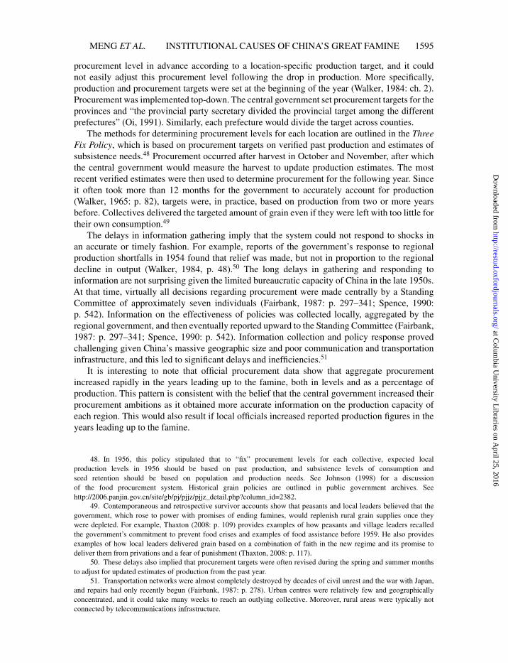
[17:16 23/4/2016 rdv016.tex] RESTUD: The Review of Economic Studies Page: 1595 1568–1611
MENG ET AL. INSTITUTIONAL CAUSES OF CHINA’S GREAT FAMINE 1595
procurement level in advance according to a location-specific production target, and it couldnot easily adjust this procurement level following the drop in production. More specifically,production and procurement targets were set at the beginning of the year (Walker, 1984: ch. 2).Procurement was implemented top-down. The central government set procurement targets for theprovinces and “the provincial party secretary divided the provincial target among the differentprefectures” (Oi, 1991). Similarly, each prefecture would divide the target across counties.
The methods for determining procurement levels for each location are outlined in the ThreeFix Policy, which is based on procurement targets on verified past production and estimates ofsubsistence needs.48 Procurement occurred after harvest in October and November, after whichthe central government would measure the harvest to update production estimates. The mostrecent verified estimates were then used to determine procurement for the following year. Sinceit often took more than 12 months for the government to accurately account for production(Walker, 1965: p. 82), targets were, in practice, based on production from two or more yearsbefore. Collectives delivered the targeted amount of grain even if they were left with too little fortheir own consumption.49
The delays in information gathering imply that the system could not respond to shocks inan accurate or timely fashion. For example, reports of the government’s response to regionalproduction shortfalls in 1954 found that relief was made, but not in proportion to the regionaldecline in output (Walker, 1984, p. 48).50 The long delays in gathering and responding toinformation are not surprising given the limited bureaucratic capacity of China in the late 1950s.At that time, virtually all decisions regarding procurement were made centrally by a StandingCommittee of approximately seven individuals (Fairbank, 1987: p. 297–341; Spence, 1990:p. 542). Information on the effectiveness of policies was collected locally, aggregated by theregional government, and then eventually reported upward to the Standing Committee (Fairbank,1987: p. 297–341; Spence, 1990: p. 542). Information collection and policy response provedchallenging given China’s massive geographic size and poor communication and transportationinfrastructure, and this led to significant delays and inefficiencies.51
It is interesting to note that official procurement data show that aggregate procurementincreased rapidly in the years leading up to the famine, both in levels and as a percentage ofproduction. This pattern is consistent with the belief that the central government increased theirprocurement ambitions as it obtained more accurate information on the production capacity ofeach region. This would also result if local officials increased reported production figures in theyears leading up to the famine.
48. In 1956, this policy stipulated that to “fix” procurement levels for each collective, expected localproduction levels in 1956 should be based on past production, and subsistence levels of consumption andseed retention should be based on population and production needs. See Johnson (1998) for a discussionof the food procurement system. Historical grain policies are outlined in public government archives. Seehttp://2006.panjin.gov.cn/site/gb/pj/pjjz/pjjz_detail.php?column_id=2382.
49. Contemporaneous and retrospective survivor accounts show that peasants and local leaders believed that thegovernment, which rose to power with promises of ending famines, would replenish rural grain supplies once theywere depleted. For example, Thaxton (2008: p. 109) provides examples of how peasants and village leaders recalledthe government’s commitment to prevent food crises and examples of food assistance before 1959. He also providesexamples of how local leaders delivered grain based on a combination of faith in the new regime and its promise todeliver them from privations and a fear of punishment (Thaxton, 2008: p. 117).
50. These delays also implied that procurement targets were often revised during the spring and summer monthsto adjust for updated estimates of production from the past year.
51. Transportation networks were almost completely destroyed by decades of civil unrest and the war with Japan,and repairs had only recently begun (Fairbank, 1987: p. 278). Urban centres were relatively few and geographicallyconcentrated, and it could take many weeks to reach an outlying collective. Moreover, rural areas were typically notconnected by telecommunications infrastructure.
at Colum
bia University L
ibraries on April 25, 2016
http://restud.oxfordjournals.org/D
ownloaded from
[17:16 23/4/2016 rdv016.tex] RESTUD: The Review of Economic Studies Page: 1596 1568–1611
1596 REVIEW OF ECONOMIC STUDIES
These fundamental limitations in bureaucratic capacity were greatly exacerbated by varioushistorical factors in the late 1950s. First, for budgetary reasons, the bureaucracy was understaffed(Eckstein, 1977: p. 186). Secondly, the Anti-Right purges in 1957 sent many able bureaucrats toreeducation in 1958, reducing the number of statisticians and demographers available to projectproduction figures in 1959 (Spence, 1990: p. 580). With diminished statistical capacity, the centralgovernment had to wait longer than usual to know the true production figures.
Thirdly, political tension during the GLF era led to an environment of suspicion and furtherreduced communication within the government. Mao and his followers were unwilling to believereports of low production from local leaders (Thaxton, 2008: p. 193–198; Dikotter, 2010). Thisreduced the effectiveness of government, and was further exacerbated by Mao’s attempts tosolidify his power by reducing the frequency of Standing Committee meetings from twice a weekto six times a year and by removing decision-making power from local governments (Fairbank,1987: p. 303). The political resistance against believing that GLF policies could potentiallyreduce production is especially important for understanding why the famine became so severeand persisted for so long. The only high-level leader known to have voiced concerns about thepossibility of famine was Peng Dehuai, China’s defence minister at the time. If the other centralleaders had believed and responded to the concerns he expressed at Lushan in July 1959, it couldhave reduced procurement in 1959 and mitigated famine mortality rates.52 However, procurementin 1959 did not take Peng’s reports into account. This was partly because many did not believethat there were production falls or increased mortality rates and argued that if these were true,they were due to lack of enforcement of the collective system rather than high procurement levels.It is possible that party leaders were genuinely over-optimistic that production would continue togrow.
Aside from limited bureaucratic capacity, one can argue that another reason for the inflexibilityof the system is that it helped the central government limit problems of asymmetric information.Relative to the central government, local leaders had much better information on the level ofproduction of their collective, but also had incentives to misreport production to the centralgovernment. Historically, local leaders often under-reported production to increase their supportamong local peasants, to retain the unreported grain for personal profit, and to suppress the centralgovernment’s expectations of future harvests (Thaxton, 2008: p. 293–312).53 Local leaders werealso known to have over-reported production when they felt pressured to meet procurementtargets or when promoting themselves politically by meeting or exceeding yield expectations.For the central government, both types of misreporting were problematic: under-reportingreduced government procurement whereas over-reporting risked government over-procurementand political instability in the countryside, which had provided the core support for the Communistparty.54 As such, there was an advantage for the central government in preserving a system inwhich local procurement levels did not solely rely on local reports. Clearly, the incentives to
52. See the Online Appendix available as Supplementary Data for a more detailed discussion of Peng Dehuai.53. The government made extensive campaigns against under-reporting. The fact that this was a prevalent problem
in the years leading up to the famine is consistent with under-reporting by local officials being included in a list of “tenevils” that was published in daily newspapers in the late 1950s (Walker, 1984: p. 65). For example, see Jilinrijipao [JilinDaily Newspaper in Chinese], 20 December 1957.
54. The government’s concerns about over-reporting is shown by the continued political discussions that localleaders should not implement “commandism” during both the first and second Five Year Plans (1953–1957, 1958–1962)(Walker, 1965: p. 8). In a meeting in Changchou in 1957, Mao personally warned party members to not commit “Stalin’smistake” in terms of over-procurement, which he believed to have turned Soviet peasants against their government(Walker, 1984: p. 149). For a detailed example, see Thaxton (2008, p. 132).
at Colum
bia University L
ibraries on April 25, 2016
http://restud.oxfordjournals.org/D
ownloaded from
[17:16 23/4/2016 rdv016.tex] RESTUD: The Review of Economic Studies Page: 1597 1568–1611
MENG ET AL. INSTITUTIONAL CAUSES OF CHINA’S GREAT FAMINE 1597
misreport production would be minimized if the central government was committed to procuringa fixed target.55
6.2. A stylized example
We construct a stylized example to explain how an inflexible procurement policy can lead to afamine in which more productive regions suffer more. Before constructing the example, it is usefulto describe the spatial pattern of the drop in production during the famine. We show that moreproductive regions typically experienced a larger absolute production drop while still remainingmore productive relative to less productive regions. Figure 5a–c plot the current year’s per capitaconstructed production for 1958–1960 against the previous year’s. The figures show that thereis little change in production ranks over time. Thus, provinces that were the most productive in1957 were still the most productive in 1958, 1959, and 1960. Figure 5d–f plot the annual growthin per capita production against the previous year’s per capita production for the three famineyears. They show a negative correlation for each year, which means that the production growthwas smaller for regions that produced more food per capita in the previous year.56 Thus, the datashow that productive provinces typically suffered larger falls in production during the famine,but not so much as to reduce their productivity rank.
Table 5 considers the implications of such a production drop together with an inflexibleprocurement policy. It provides an example of a country with three hypothetical regions: tworural regions (A and B) and a city. Each region has a similar population, and therefore similarsubsistence needs. For simplicity, we assume the latter to be 100 tons of food. However,agricultural endowments differ across regions. A is better endowed than B, and hence producesmore food per capita. The city produces no food. As was the case in China, the governmentrestricts population movements so that individuals from low production regions cannot move tohigh production regions.
There are two states of the world. In the normal state, which occurs with 80% probability, Aproduces 250 tons and B produces 170 tons. The second state is caused by an aggregate shockwhich occurs with 20% probability, and production is 20% lower for each region, reducingproduction in A and B to 200 and 136 tons.57 The government expects the aggregate shock tooccur with 20% probability. The key feature of this production shock is that it is rank preserving,but at the same time, more productive regions experience larger falls in production. It follows thatexpected production of A and B are 240 (250×0.8+200×0.2) and 163 (170×0.8+136×0.2)tons, which sum to 403 tons of total production.
In accordance with the anecdotal evidence that the grain procurement policy was inflexible, thegovernment consistently procures a fixed amount from each region in all states of the world. Sincewe do not know the precise historical objective function of the Chinese government, we assume forsimplicity that the government chooses procurement to equalize expected consumption across itscitizens, giving each of the three regions 134 tons of expected consumption. Thus, the governmentconsistently procures the difference between expected production and expected consumption in
55. This idea can be easily formalized in a mechanism design framework in a setting where the planner tries toinduce an agent with a preference for misreporting to truthfully reveal the amount produced. See an earlier version ofthis article (Meng et al. 2010).
56. The data exhibit similar patterns if we compare current production to a lagged moving average of production.Also, reported production data exhibit similar patterns. These figures are available upon request.
57. We assume a proportional drop in production in this stylized example for simplicity since it produces a similarpattern to what we see in the data: more productive provinces would suffer a larger magnitude drop in production, butproductivity ranks across provinces will not change.
at Colum
bia University L
ibraries on April 25, 2016
http://restud.oxfordjournals.org/D
ownloaded from
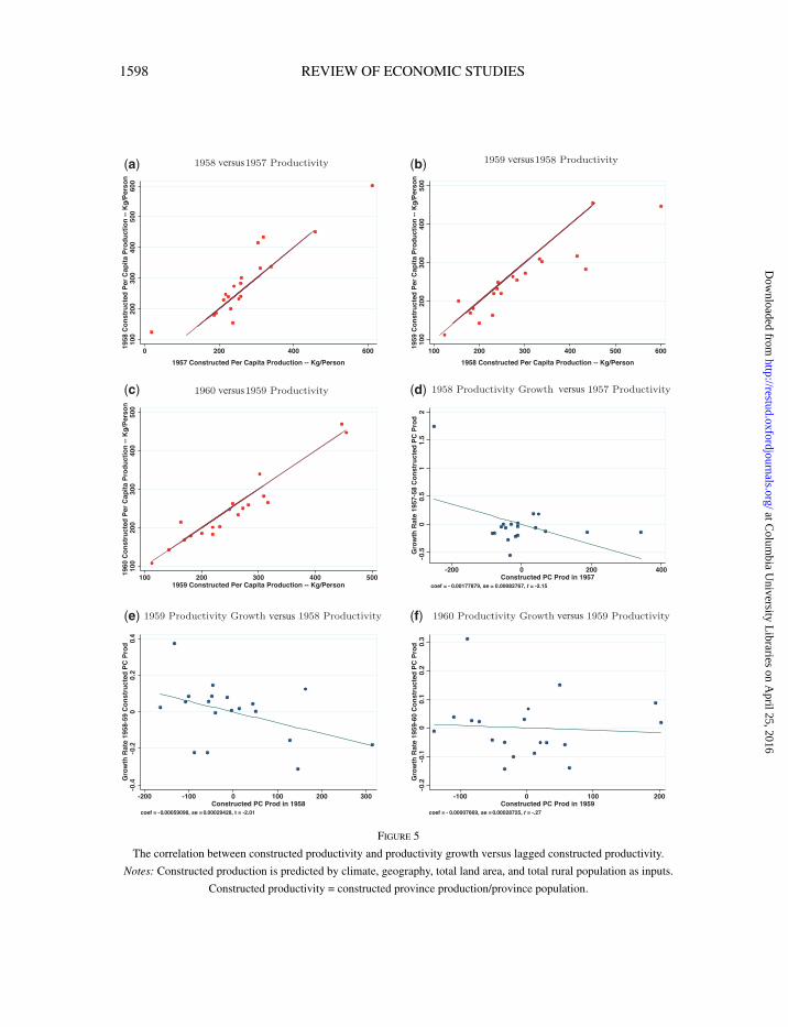
[17:16 23/4/2016 rdv016.tex] RESTUD: The Review of Economic Studies Page: 1598 1568–1611
1598 REVIEW OF ECONOMIC STUDIES
(a) (b)
(c) (d)
(e) (f)
versus
versus versus
versusversus
versus
Figure 5
The correlation between constructed productivity and productivity growth versus lagged constructed productivity.
Notes: Constructed production is predicted by climate, geography, total land area, and total rural population as inputs.
Constructed productivity = constructed province production/province population.
at Colum
bia University L
ibraries on April 25, 2016
http://restud.oxfordjournals.org/D
ownloaded from
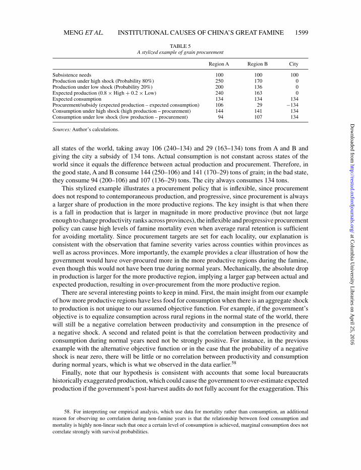
[17:16 23/4/2016 rdv016.tex] RESTUD: The Review of Economic Studies Page: 1599 1568–1611
MENG ET AL. INSTITUTIONAL CAUSES OF CHINA’S GREAT FAMINE 1599
TABLE 5A stylized example of grain procurement
Region A Region B City
Subsistence needs 100 100 100Production under high shock (Probability 80%) 250 170 0Production under low shock (Probability 20%) 200 136 0Expected production (0.8 × High + 0.2 × Low) 240 163 0Expected consumption 134 134 134Procurement/subsidy (expected production – expected consumption) 106 29 −134Consumption under high shock (high production – procurement) 144 141 134Consumption under low shock (low production – procurement) 94 107 134
Sources: Author’s calculations.
all states of the world, taking away 106 (240–134) and 29 (163–134) tons from A and B andgiving the city a subsidy of 134 tons. Actual consumption is not constant across states of theworld since it equals the difference between actual production and procurement. Therefore, inthe good state, A and B consume 144 (250–106) and 141 (170–29) tons of grain; in the bad state,they consume 94 (200–106) and 107 (136–29) tons. The city always consumes 134 tons.
This stylized example illustrates a procurement policy that is inflexible, since procurementdoes not respond to contemporaneous production, and progressive, since procurement is alwaysa larger share of production in the more productive regions. The key insight is that when thereis a fall in production that is larger in magnitude in more productive province (but not largeenough to change productivity ranks across provinces), the inflexible and progressive procurementpolicy can cause high levels of famine mortality even when average rural retention is sufficientfor avoiding mortality. Since procurement targets are set for each locality, our explanation isconsistent with the observation that famine severity varies across counties within provinces aswell as across provinces. More importantly, the example provides a clear illustration of how thegovernment would have over-procured more in the more productive regions during the famine,even though this would not have been true during normal years. Mechanically, the absolute dropin production is larger for the more productive region, implying a larger gap between actual andexpected production, resulting in over-procurement from the more productive region.
There are several interesting points to keep in mind. First, the main insight from our exampleof how more productive regions have less food for consumption when there is an aggregate shockto production is not unique to our assumed objective function. For example, if the government’sobjective is to equalize consumption across rural regions in the normal state of the world, therewill still be a negative correlation between productivity and consumption in the presence ofa negative shock. A second and related point is that the correlation between productivity andconsumption during normal years need not be strongly positive. For instance, in the previousexample with the alternative objective function or in the case that the probability of a negativeshock is near zero, there will be little or no correlation between productivity and consumptionduring normal years, which is what we observed in the data earlier.58
Finally, note that our hypothesis is consistent with accounts that some local bureaucratshistorically exaggerated production, which could cause the government to over-estimate expectedproduction if the government’s post-harvest audits do not fully account for the exaggeration. This
58. For interpreting our empirical analysis, which use data for mortality rather than consumption, an additionalreason for observing no correlation during non-famine years is that the relationship between food consumption andmortality is highly non-linear such that once a certain level of consumption is achieved, marginal consumption does notcorrelate strongly with survival probabilities.
at Colum
bia University L
ibraries on April 25, 2016
http://restud.oxfordjournals.org/D
ownloaded from
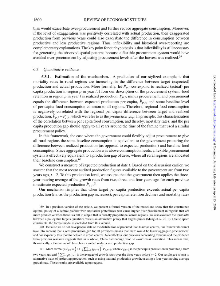
[17:16 23/4/2016 rdv016.tex] RESTUD: The Review of Economic Studies Page: 1600 1568–1611
1600 REVIEW OF ECONOMIC STUDIES
bias would exacerbate over-procurement and further reduce aggregate consumption. Moreover,if the level of exaggeration was positively correlated with actual production, then exaggeratedproduction from previous years could also exacerbate the difference in consumption betweenproductive and less productive regions. Thus, inflexibility and historical over-reporting arecomplementary explanations. The key point for our hypothesis is that inflexibility is still necessaryfor generating the observed spatial patterns because a flexible procurement system would haveavoided over-procurement by adjusting procurement levels after the harvest was realized.59
6.3. Quantitative evidence
6.3.1. Estimation of the mechanism. A prediction of our stylized example is thatmortality rates in rural regions are increasing in the difference between target (expected)production and actual production. More formally, let Pp,t correspond to realized (actual) percapita production in region p in year t. From our description of the procurement system, foodretention in region p in year t is realized production, Pp,t , minus procurement, and procurementequals the difference between expected production per capita, P̂p,t , and some baseline levelof per capita food consumption common to all regions. Therefore, regional food consumptionis negatively correlated with the regional per capita difference between target and realizedproduction, P̂p,t −Pp,t , which we refer to as the production gap. In principle, this characterizationof the correlation between per capita food consumption, and thereby, mortality rates, and the percapita production gap should apply to all years around the time of the famine that used a similarprocurement policy.
In this framework, the case where the government could flexibly adjust procurement to giveall rural regions the same baseline consumption is equivalent to the government procuring thedifference between realized production (as opposed to expected production) and baseline foodconsumption. Since aggregate production was above consumption needs, a flexible procurementsystem is effectively equivalent to a production gap of zero, where all rural regions are allocatedtheir baseline consumption.60
We construct a measure of expected production at date t. Based on the discussion earlier, weassume that the most recent audited production figures available to the government are from twoyears ago, t−2. To this production level, we assume that the government then applies the three-year moving average of the growth rates from two, three, and four years ago for each provinceto estimate expected production P̂p,t .61
Our mechanism implies that when target per capita production exceeds actual per capitaproduction (i.e. as the production gap increases), per capita retention declines and mortality rates
59. In a previous version of the article, we present a formal version of the model and show that the constrainedoptimal policy of a central planner with utilitarian preferences will cause higher over-procurement in regions that aremore productive when there is a fall in output that is broadly proportional across regions. We also evaluate the trade-offsbetween a policy that targets quantities versus an alternative policy that targets prices (Meng et al. 2010). Due to spaceconstraints, the formal model is excluded from this version.
60. Because we do not have precise data on the distribution of procured food to urban centres, our framework cannottake into account that a zero production gap for all provinces means that there would be lower aggregate procurement,and consequently less food to deliver to urban centres. Nevertheless, our previous accounting exercise and the evidencefrom previous research suggests that as a whole, China had enough food to avoid mass starvation. This means that,theoretically, a famine would have been avoided under a zero production gap.
61. More formally, P̂p,t =(
1+ 13
∑4τ=2 gp,t−τ
)2Pp,t−2, where Pp,t−2 is the per capita production in province p from
two years ago and 13
∑4τ=2 gp,t−τ is the average of growth rates over the three years before t−2. Our results are robust to
alternative ways of projecting production, such as using national production growth, or using a four-year moving averagegrowth rate. These results are available upon request.
at Colum
bia University L
ibraries on April 25, 2016
http://restud.oxfordjournals.org/D
ownloaded from
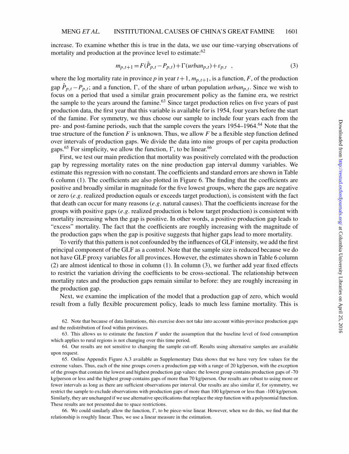
[17:16 23/4/2016 rdv016.tex] RESTUD: The Review of Economic Studies Page: 1601 1568–1611
MENG ET AL. INSTITUTIONAL CAUSES OF CHINA’S GREAT FAMINE 1601
increase. To examine whether this is true in the data, we use our time-varying observations ofmortality and production at the province level to estimate:62
mp,t+1 =F(P̂p,t −Pp,t)+�(urbanp,t)+εp,t , (3)
where the log mortality rate in province p in year t+1, mp,t+1, is a function, F, of the productiongap P̂p,t −Pp,t ; and a function, �, of the share of urban population urbanp,t . Since we wish tofocus on a period that used a similar grain procurement policy as the famine era, we restrictthe sample to the years around the famine.63 Since target production relies on five years of pastproduction data, the first year that this variable is available for is 1954, four years before the startof the famine. For symmetry, we thus choose our sample to include four years each from thepre- and post-famine periods, such that the sample covers the years 1954–1964.64 Note that thetrue structure of the function F is unknown. Thus, we allow F be a flexible step function definedover intervals of production gaps. We divide the data into nine groups of per capita productiongaps.65 For simplicity, we allow the function, �, to be linear.66
First, we test our main prediction that mortality was positively correlated with the productiongap by regressing mortality rates on the nine production gap interval dummy variables. Weestimate this regression with no constant. The coefficients and standard errors are shown in Table6 column (1). The coefficients are also plotted in Figure 6. The finding that the coefficients arepositive and broadly similar in magnitude for the five lowest groups, where the gaps are negativeor zero (e.g. realized production equals or exceeds target production), is consistent with the factthat death can occur for many reasons (e.g. natural causes). That the coefficients increase for thegroups with positive gaps (e.g. realized production is below target production) is consistent withmortality increasing when the gap is positive. In other words, a positive production gap leads to“excess” mortality. The fact that the coefficients are roughly increasing with the magnitude ofthe production gaps when the gap is positive suggests that higher gaps lead to more mortality.
To verify that this pattern is not confounded by the influences of GLF intensity, we add the firstprincipal component of the GLF as a control. Note that the sample size is reduced because we donot have GLF proxy variables for all provinces. However, the estimates shown in Table 6 column(2) are almost identical to those in column (1). In column (3), we further add year fixed effectsto restrict the variation driving the coefficients to be cross-sectional. The relationship betweenmortality rates and the production gaps remain similar to before: they are roughly increasing inthe production gap.
Next, we examine the implication of the model that a production gap of zero, which wouldresult from a fully flexible procurement policy, leads to much less famine mortality. This is
62. Note that because of data limitations, this exercise does not take into account within-province production gapsand the redistribution of food within provinces.
63. This allows us to estimate the function F under the assumption that the baseline level of food consumptionwhich applies to rural regions is not changing over this time period.
64. Our results are not sensitive to changing the sample cut-off. Results using alternative samples are availableupon request.
65. Online Appendix Figure A.3 available as Supplementary Data shows that we have very few values for theextreme values. Thus, each of the nine groups covers a production gap with a range of 20 kg/person, with the exceptionof the groups that contain the lowest and highest production gap values: the lowest group contains production gaps of -70kg/person or less and the highest group contains gaps of more than 70 kg/person. Our results are robust to using more orfewer intervals as long as there are sufficient observations per interval. Our results are also similar if, for symmetry, werestrict the sample to exclude observations with production gaps of more than 100 kg/person or less than -100 kg/person.Similarly, they are unchanged if we use alternative specifications that replace the step function with a polynomial function.These results are not presented due to space restrictions.
66. We could similarly allow the function, �, to be piece-wise linear. However, when we do this, we find that therelationship is roughly linear. Thus, we use a linear measure in the estimation.
at Colum
bia University L
ibraries on April 25, 2016
http://restud.oxfordjournals.org/D
ownloaded from
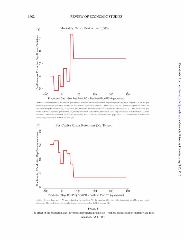
[17:16 23/4/2016 rdv016.tex] RESTUD: The Review of Economic Studies Page: 1602 1568–1611
1602 REVIEW OF ECONOMIC STUDIES
(a)
(b)
1
Figure 6
The effect of the production gap (government projected production—realized production) on mortality and food
retention, 1954–1964
at Colum
bia University L
ibraries on April 25, 2016
http://restud.oxfordjournals.org/D
ownloaded from
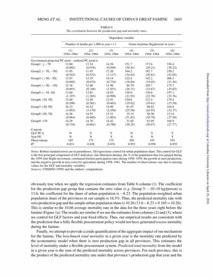
[17:16 23/4/2016 rdv016.tex] RESTUD: The Review of Economic Studies Page: 1603 1568–1611
MENG ET AL. INSTITUTIONAL CAUSES OF CHINA’S GREAT FAMINE 1603
TABLE 6The correlation between the production gap and mortality rates
Dependent variable
Number of deaths per 1,000 in year t+1 Grain retention (Kg/person) in year t
(1) (2) (3) (4) (5) (6)1954–1964 1954–1964 1954–1964 1954–1964 1954–1964 1954–1964
Government projected PC prod – realized PC prod isGroup1: ≤−70 13.00 13.34 14.26 151.7 173.6 226.4
(0.802) (0.978) (0.949) (30.41) (29.21) (39.22)Group2: (−70, −50] 11.85 11.93 12.20 164.2 182.7 230.2
(0.542) (0.532) (1.117) (34.42) (36.81) (42.85)Group3: (−50,−30] 13.07 13.35 14.14 122.4 142.2 206.1
(0.602) (0.674) (0.734) (18.84) (19.03) (31.54)Group4: (−30, −10] 12.18 12.40 11.96 84.70 105.7 175.7
(0.691) (0.746) (1.031) (26.31) (23.67) (35.02)Group5: (−10, 10] 13.60 13.83 14.03 130.0 138.6 197.1
(1.197) (1.265) (0.998) (21.93) (22.70) (32.76)Group6: (10, 30] 12.60 12.49 12.93 120.8 123.4 179.4
(0.509) (0.501) (0.665) (19.92) (19.61) (33.50)Group7: (30, 50] 16.33 16.52 14.90 81.97 98.82 164.6
(3.093) (3.179) (2.458) (25.50) (24.93) (32.37)Group8: (50, 70] 14.36 14.55 15.31 35.15 56.38 113.6
(0.964) (0.969) (1.003) (31.83) (29.79) (37.58)Group9: >70 14.29 14.70 14.42 31.85 63.05 104.9
(0.718) (0.861) (0.788) (30.25) (29.67) (27.77)
ControlsGLF PCA N Y Y N Y YYear FE N N Y N N YObservations 185 175 175 204 193 193R2 0.831 0.828 0.876 0.953 0.950 0.955
Notes: Robust standard errors are in parentheses. All regressions control for urban population share. The control for GLFis the first principal component of GLF indicators: late liberation dummy, the % of the population that was purged duringthe 1959 Anti-Right movement, communal kitchen participation rates during 1958–1959, the growth in steel production,and the negative growth in area sown for agriculture during 1958–1961. The number of observations vary due to missingvalues for the GLF and mortality variables.Sources: CDSM50 (1999) and the authors’ computations.
obviously true when we apply the regression estimates from Table 6 column (1). The coefficientfor the production gap group that contains the zero value (e.g. Group 5: −10–10 kg/person) is13.6, the coefficient for the share of urban population is −8.23. The population-weighted urbanpopulation share of the provinces in our sample is 16.5%. Thus, the predicted mortality rate withzero production gap and the sample urban population share is 10.26 (13.6−8.23×0.165=10.26).This is similar to the 10.66 average mortality rate in the data for the three years right before thefamine (Figure 1a). The results are similar if we use the estimates from columns (2) and (3), wherewe control for GLF factors and year fixed effects. Thus, our empirical results are consistent withthe prediction that a fully flexible procurement policy would not have generated excess mortalityduring the famine.
Finally, we attempt to provide a crude quantification of the aggregate impact of our mechanismfor the famine. The benchmark total mortality in a given year is the mortality rate predicted bythe econometric model when there is zero production gap in all provinces. This estimates thelevel of mortality under a flexible procurement system. Predicted total mortality from the modelin a given year is the sum of the predicted mortality across provinces. For each province, this isthe product of the predicted mortality rate under that province’s production gap that year and the
at Colum
bia University L
ibraries on April 25, 2016
http://restud.oxfordjournals.org/D
ownloaded from
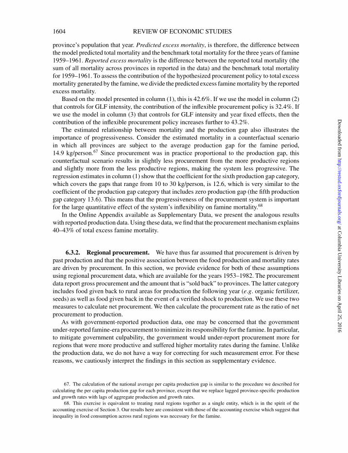
[17:16 23/4/2016 rdv016.tex] RESTUD: The Review of Economic Studies Page: 1604 1568–1611
1604 REVIEW OF ECONOMIC STUDIES
province’s population that year. Predicted excess mortality, is therefore, the difference betweenthe model predicted total mortality and the benchmark total mortality for the three years of famine1959–1961. Reported excess mortality is the difference between the reported total mortality (thesum of all mortality across provinces in reported in the data) and the benchmark total mortalityfor 1959–1961. To assess the contribution of the hypothesized procurement policy to total excessmortality generated by the famine, we divide the predicted excess famine mortality by the reportedexcess mortality.
Based on the model presented in column (1), this is 42.6%. If we use the model in column (2)that controls for GLF intensity, the contribution of the inflexible procurement policy is 32.4%. Ifwe use the model in column (3) that controls for GLF intensity and year fixed effects, then thecontribution of the inflexible procurement policy increases further to 43.2%.
The estimated relationship between mortality and the production gap also illustrates theimportance of progressiveness. Consider the estimated mortality in a counterfactual scenarioin which all provinces are subject to the average production gap for the famine period,14.9 kg/person.67 Since procurement was in practice proportional to the production gap, thiscounterfactual scenario results in slightly less procurement from the more productive regionsand slightly more from the less productive regions, making the system less progressive. Theregression estimates in column (1) show that the coefficient for the sixth production gap category,which covers the gaps that range from 10 to 30 kg/person, is 12.6, which is very similar to thecoefficient of the production gap category that includes zero production gap (the fifth productiongap category 13.6). This means that the progressiveness of the procurement system is importantfor the large quantitative effect of the system’s inflexibility on famine mortality.68
In the Online Appendix available as Supplementary Data, we present the analogous resultswith reported production data. Using these data, we find that the procurement mechanism explains40–43% of total excess famine mortality.
6.3.2. Regional procurement. We have thus far assumed that procurement is driven bypast production and that the positive association between the food production and mortality ratesare driven by procurement. In this section, we provide evidence for both of these assumptionsusing regional procurement data, which are available for the years 1953–1982. The procurementdata report gross procurement and the amount that is “sold back” to provinces. The latter categoryincludes food given back to rural areas for production the following year (e.g. organic fertilizer,seeds) as well as food given back in the event of a verified shock to production. We use these twomeasures to calculate net procurement. We then calculate the procurement rate as the ratio of netprocurement to production.
As with government-reported production data, one may be concerned that the governmentunder-reported famine-era procurement to minimize its responsibility for the famine. In particular,to mitigate government culpability, the government would under-report procurement more forregions that were more productive and suffered higher mortality rates during the famine. Unlikethe production data, we do not have a way for correcting for such measurement error. For thesereasons, we cautiously interpret the findings in this section as supplementary evidence.
67. The calculation of the national average per capita production gap is similar to the procedure we described forcalculating the per capita production gap for each province, except that we replace lagged province-specific productionand growth rates with lags of aggregate production and growth rates.
68. This exercise is equivalent to treating rural regions together as a single entity, which is in the spirit of theaccounting exercise of Section 3. Our results here are consistent with those of the accounting exercise which suggest thatinequality in food consumption across rural regions was necessary for the famine.
at Colum
bia University L
ibraries on April 25, 2016
http://restud.oxfordjournals.org/D
ownloaded from
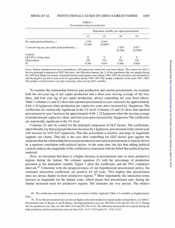
[17:16 23/4/2016 rdv016.tex] RESTUD: The Review of Economic Studies Page: 1605 1568–1611
MENG ET AL. INSTITUTIONAL CAUSES OF CHINA’S GREAT FAMINE 1605
TABLE 7Procurement and past production
Dependent variable: per capita procurementt
(1) (2) (4) (5)
Per capita grain productiont−2 1.238 0.643(0.106) (0.0687)
3 year moving avg. per capita grain productiont−2 1.250 0.677(0.104) (0.0704)
ControlsGLF PCA, Urban share N Y N YObservations 228 216 228 216R2 0.396 0.835 0.408 0.838
Notes: Robust standard errors are in parentheses. All regressions control for year fixed effects. The control for GLF isthe first principal component of GLF indicators: late liberation dummy, the % of the population that was purged duringthe 1959 Anti-Right movement, communal kitchen participation rates during 1958–1959, the growth in steel production,and the negative growth in area sown for agriculture during 1958–1961.The sample comprises of the years 1953–1964.The number of observations vary due to missing values for the GLF variables.
To examine the relationship between past production and current procurement, we examineboth the two-year lag of per capita production and a three-year moving average of the two,three, and four year lag of per capita production, always controlling for year fixed effects.Table 7 columns (1) and (2) show that reported procurement in year t increases by approximately0.64–1.24 kg/person when production per capita two years prior increased by 1kg/person. Thecoefficients are statistically significant at the 1% level. Columns (3) and (4) show that reportedprocurement in year t increases by approximately 0.68–1.25 kg/person when the moving averageof production per capita two, three, and four years prior increased by 1kg/person. The coefficientsare statistically significant at the 1% level.
Columns (2) and (4) control for the principal component of GLF factors. The coefficients,taken literally, say that as past production increases by 1 kg/person, procurement in the current yearwill increase by 0.65–0.67 kg/person. That this association is positive and large in magnitudesupports our claims. That this is the case after controlling for GLF factors goes against thesuspicion that the relationship between past production and current procurement is entirely drivenby a spurious correlation with political factors. At the same time, the fact that adding politicalcontrols reduces the magnitude of the coefficient is consistent with the belief that political factorsmattered.
Next, we document that there is a higher increase in procurement rates in more productiveregions during the famine. We estimate equation (2) with the percentage of productionprocured as the dependent variable. Figure 7 plots the coefficients and the 95% confidenceintervals.69 Consistent with the progressiveness of our hypothesized procurement policy, theestimated interaction coefficients are positive for all years. This implies that procurementrates are always higher in more productive regions.70 More importantly, the interaction termsincrease in magnitude for the famine years, which means that procurement rates during thefamine increased more for productive regions. The estimates are very precise. The relative
69. The coefficients and standard errors are presented in Online Appendix Table A.3 available as SupplementaryData.
70. To see that procurement rates are always higher in the more productive regions under our hypothesis, see Table 5.Procurement rates in Region A and B during a the high production year are 106/250=0.42 and 29/170=0.17. Duringthe low production year, they are 106/200=0.53 and 29/136=0.21. The difference between the two regions during thehigh production and low production years are thus 0.42−0.17=0.25 and 0.53−0.21=0.31.
at Colum
bia University L
ibraries on April 25, 2016
http://restud.oxfordjournals.org/D
ownloaded from
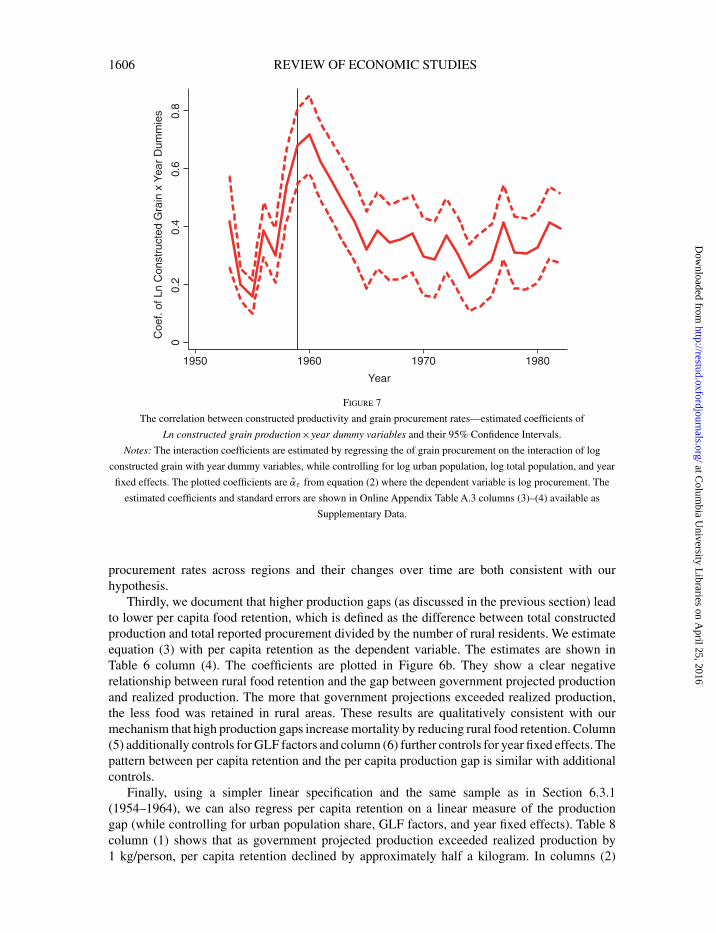
[17:16 23/4/2016 rdv016.tex] RESTUD: The Review of Economic Studies Page: 1606 1568–1611
1606 REVIEW OF ECONOMIC STUDIES
00.
20.
40.
60.
8
Coe
f. of
Ln
Con
stru
cted
Gra
in x
Yea
r D
umm
ies
1950 1960 1970 1980
Year
Figure 7
The correlation between constructed productivity and grain procurement rates—estimated coefficients of
Ln constructed grain production×year dummy variables and their 95% Confidence Intervals.
Notes: The interaction coefficients are estimated by regressing the of grain procurement on the interaction of log
constructed grain with year dummy variables, while controlling for log urban population, log total population, and year
fixed effects. The plotted coefficients are α̂τ from equation (2) where the dependent variable is log procurement. The
estimated coefficients and standard errors are shown in Online Appendix Table A.3 columns (3)–(4) available as
Supplementary Data.
procurement rates across regions and their changes over time are both consistent with ourhypothesis.
Thirdly, we document that higher production gaps (as discussed in the previous section) leadto lower per capita food retention, which is defined as the difference between total constructedproduction and total reported procurement divided by the number of rural residents. We estimateequation (3) with per capita retention as the dependent variable. The estimates are shown inTable 6 column (4). The coefficients are plotted in Figure 6b. They show a clear negativerelationship between rural food retention and the gap between government projected productionand realized production. The more that government projections exceeded realized production,the less food was retained in rural areas. These results are qualitatively consistent with ourmechanism that high production gaps increase mortality by reducing rural food retention. Column(5) additionally controls for GLF factors and column (6) further controls for year fixed effects. Thepattern between per capita retention and the per capita production gap is similar with additionalcontrols.
Finally, using a simpler linear specification and the same sample as in Section 6.3.1(1954–1964), we can also regress per capita retention on a linear measure of the productiongap (while controlling for urban population share, GLF factors, and year fixed effects). Table 8column (1) shows that as government projected production exceeded realized production by1 kg/person, per capita retention declined by approximately half a kilogram. In columns (2)
at Colum
bia University L
ibraries on April 25, 2016
http://restud.oxfordjournals.org/D
ownloaded from
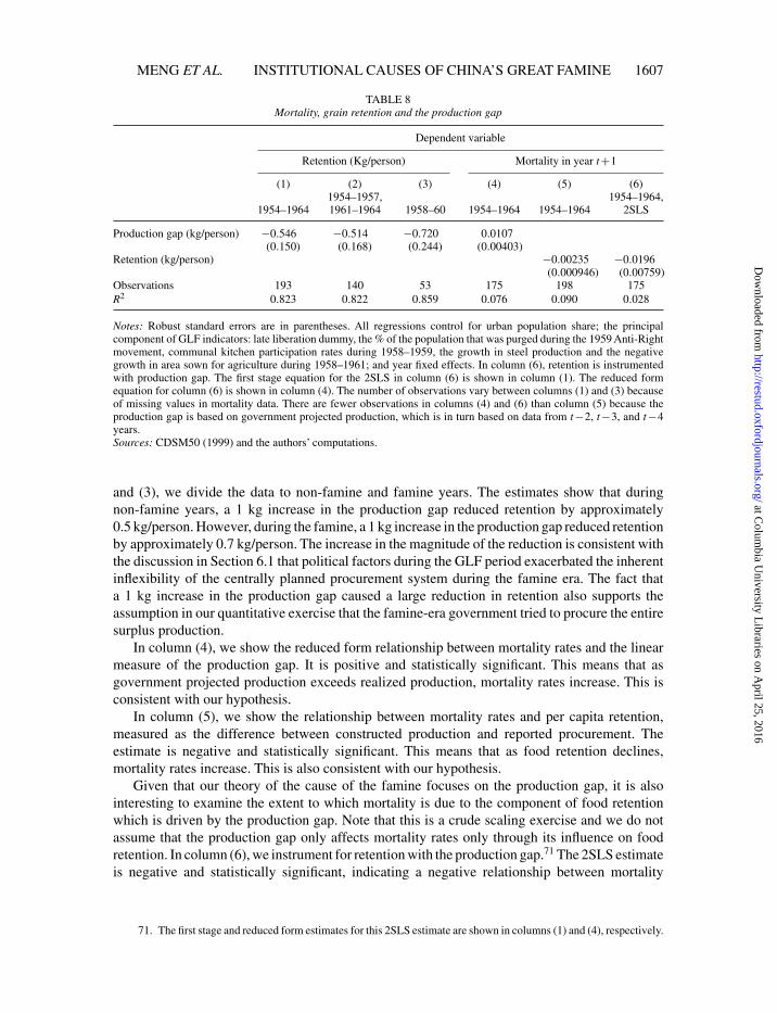
[17:16 23/4/2016 rdv016.tex] RESTUD: The Review of Economic Studies Page: 1607 1568–1611
MENG ET AL. INSTITUTIONAL CAUSES OF CHINA’S GREAT FAMINE 1607
TABLE 8Mortality, grain retention and the production gap
Dependent variable
Retention (Kg/person) Mortality in year t+1
(1) (2) (3) (4) (5) (6)1954–1957, 1954–1964,
1954–1964 1961–1964 1958–60 1954–1964 1954–1964 2SLS
Production gap (kg/person) −0.546 −0.514 −0.720 0.0107(0.150) (0.168) (0.244) (0.00403)
Retention (kg/person) −0.00235 −0.0196(0.000946) (0.00759)
Observations 193 140 53 175 198 175R2 0.823 0.822 0.859 0.076 0.090 0.028
Notes: Robust standard errors are in parentheses. All regressions control for urban population share; the principalcomponent of GLF indicators: late liberation dummy, the % of the population that was purged during the 1959 Anti-Rightmovement, communal kitchen participation rates during 1958–1959, the growth in steel production and the negativegrowth in area sown for agriculture during 1958–1961; and year fixed effects. In column (6), retention is instrumentedwith production gap. The first stage equation for the 2SLS in column (6) is shown in column (1). The reduced formequation for column (6) is shown in column (4). The number of observations vary between columns (1) and (3) becauseof missing values in mortality data. There are fewer observations in columns (4) and (6) than column (5) because theproduction gap is based on government projected production, which is in turn based on data from t−2, t−3, and t−4years.Sources: CDSM50 (1999) and the authors’ computations.
and (3), we divide the data to non-famine and famine years. The estimates show that duringnon-famine years, a 1 kg increase in the production gap reduced retention by approximately0.5 kg/person. However, during the famine, a 1 kg increase in the production gap reduced retentionby approximately 0.7 kg/person. The increase in the magnitude of the reduction is consistent withthe discussion in Section 6.1 that political factors during the GLF period exacerbated the inherentinflexibility of the centrally planned procurement system during the famine era. The fact thata 1 kg increase in the production gap caused a large reduction in retention also supports theassumption in our quantitative exercise that the famine-era government tried to procure the entiresurplus production.
In column (4), we show the reduced form relationship between mortality rates and the linearmeasure of the production gap. It is positive and statistically significant. This means that asgovernment projected production exceeds realized production, mortality rates increase. This isconsistent with our hypothesis.
In column (5), we show the relationship between mortality rates and per capita retention,measured as the difference between constructed production and reported procurement. Theestimate is negative and statistically significant. This means that as food retention declines,mortality rates increase. This is also consistent with our hypothesis.
Given that our theory of the cause of the famine focuses on the production gap, it is alsointeresting to examine the extent to which mortality is due to the component of food retentionwhich is driven by the production gap. Note that this is a crude scaling exercise and we do notassume that the production gap only affects mortality rates only through its influence on foodretention. In column (6), we instrument for retention with the production gap.71 The 2SLS estimateis negative and statistically significant, indicating a negative relationship between mortality
71. The first stage and reduced form estimates for this 2SLS estimate are shown in columns (1) and (4), respectively.
at Colum
bia University L
ibraries on April 25, 2016
http://restud.oxfordjournals.org/D
ownloaded from
[17:16 23/4/2016 rdv016.tex] RESTUD: The Review of Economic Studies Page: 1608 1568–1611
1608 REVIEW OF ECONOMIC STUDIES
and food retention. This is again consistent with our hypothesis that as government projectedproduction exceeds realized production, food retention declines and mortality increases.
We interpret the results in this section as evidence in support of our mechanism. At thesame time, we conservatively interpret the quantitative magnitudes as illustrative. Note that sincemortality is a non-linear function of consumption and there is significant variation in retentionlevels within a province, the coefficients cannot be interpreted as an elasticity of mortality withrespect to consumption.
In the Online Appendix available as Supplementary Data, we present analogous results usingreported production data. The findings that retention is decreasing in the production gap and thathigher retention reduces mortality rates are similar.
7. CONCLUSION
During the 20th century, millions have perished from famine, and over 60% of total faminemortality has occurred in centrally planned economies. The most deadly famine in history wasthe Chinese Great Famine, which in just a few years, killed up to 45 million individuals. Thisarticle proposes that an inflexible and progressive government procurement policy is necessaryfor explaining the famine. Other explanations for the famine cannot be easily reconciled withthe patterns of rural inequality in famine that we document, and the presence of rural inequalityis necessary to generate such a massive famine given high average rural food availability. Ourresults show that the inflexible and progressive procurement policy contributed to 32–43% oftotal famine mortality. This means that our mechanism is quantitatively important. At the sametime, it leaves much room for the contribution of other factors for famine mortality, such asthe political factors that have been previously emphasized by famine scholars. Another way ofinterpreting our results is to say that absent these other factors, famine mortality could have been57–68% lower.
There are several important points to keep in mind for understanding the role of inflexibilityin causing the famine. The inability to aggregate information about true production would nothave only caused the the government to over-procure, but it also delayed its ability to respond tofamine by sending replenishments back to the affected regions. Given the data limitations, we areunable to distinguish the effect of over-procurement from the effect of delayed replenishments.Both effects are captured in our reduced form analysis and contribute to our back-of-the-envelopecalculations of the quantitative contribution of inflexible procurement.
Our results do not mean that inflexible procurement must lead to famine. In the Chinesecontext, inflexible procurement caused a famine because the government miscalculated grainprojections while aiming to procure an extremely large proportion of surplus production.After thefamine, perhaps with the realization that some degree of government miscalculation is inevitable,the government lowered the procurement rate. As long as the government was committed toits inflexible procurement regime, lowering aggregate procurement goals was the only policyinstrument available for avoiding another famine.
Thus, our theory of the cause of the famine has different policy implications from the theorieshighlighted in previous studies, which have mostly focused on the zealous pursuit of misguidedGLF policies. If one believes that the main contributor was bad GLF policies and politicalradicalism during the late 1950s, then China would have no more famines once GLF policieswere abandoned. In contrast, if one believes that inflexibility was an important contributor, thenthe Chinese government would have had to take additional measures, or risk another famine(albeit one of smaller magnitude if political radicalism has subsided) the next time there was anunanticipated production shock. The fact that the government permanently reduced procurement
at Colum
bia University L
ibraries on April 25, 2016
http://restud.oxfordjournals.org/D
ownloaded from
[17:16 23/4/2016 rdv016.tex] RESTUD: The Review of Economic Studies Page: 1609 1568–1611
MENG ET AL. INSTITUTIONAL CAUSES OF CHINA’S GREAT FAMINE 1609
rates after GLF policies were abandoned suggests that post-famine Chinese policymakers mayhave understood the risks inherent to an inflexible system.
It is important to note that the context of our study has many specific institutional features, andat the same time recognize that the inflexibility we describe stems from the fundamental problemof mistrust—farmers, who must give all surplus production to the government, do not have thecorrect incentives to truthfully report production and local bureaucrats may under- or over-reportproduction depending on whether they curry the favour of their neighbours or the officials in theupper levels of government. The problem we highlight is, therefore, a generic problem for anyregime where the farmer is not the residual claimant of his production.
The most essential ingredients for our mechanism—the commitment to central planning,the incentives for regional bureaucrats and peasants to misreport production and to shirk, theinability to quickly aggregate, and respond to new information—are common to several othercentrally planned economies of the 20th century. For example, we believe that our study providespotentially generalizable insights for understanding the causes of the Soviet Famine during1932–1933, which killed up to 6.5 million people in just one year (Davies and Wheatcroft, 2004).There is a consensus that high government procurement from rural areas caused the famine. Likethe Chinese case, the most conservative estimates of rural retention in the most severely strickenSoviet state, the Ukraine, show that average rural food availability after procurement was deductedwas approximately 170 kg/person during the worst year of the famine (Conquest, 1987). Thisprovides a diet of approximately 1,671 calories per day. While it is not a rich diet, it is muchmore than the level needed to avoid the high famine mortality rates experienced by the Ukraine.Also, as in the case of China, the data suggest similar spatial patterns in mortality rates—they arehigher in more productive regions.72
These provocative similarities suggest that the role of the inflexible procurement policy inother historical famines like the Soviet Famine is a worthy topic of future research. Similarly, it isalso important to develop a more generalized framework for understanding the conditions underwhich rigid food distribution mechanisms in centrally planned economies contribute to famine.The evidence offered in this study takes a first step in this agenda.
Acknowledgments. We are indebted to Francesco Caselli, an anonymous co-editor and seven anonymous refereesfor invaluable suggestions. We also thank Daron Acemoglu, Alberto Alesina, Abhijit Banerjee, Robin Burgess, ClaudiaGoldin, Mikhail Golosov, Rick Hornbeck, Chang-tai Hsieh, Dean Karlan, Michael Kremer, James Kung, NaomiLamoureaux, Christopher Leighton, Cormac O’Grada, Suresh Naidu, Emi Nakamura, Nathan Nunn, Gerard Padro-i-Miquel, Chris Udry, Dennis Yang and Fabrizio Zillibotti for their comments; the participants at the Berkeley DevelopmentSeminar, Kiel Institute of International Economics, UCLA Applied Economics Seminar, Stanford Economic HistorySeminar, University of Texas at Austin Applied Micro Seminar, University of Toronto Applied Micro Seminar, TsinghuaUniversity Economics Seminar, theApplied Workshop at CCER PKU, the Economics Workshop at Hong Kong University,the Applied Micro Seminar at the Chinese University of Hong Kong, Yale University Macro Lunch and HarvardHistory Tea, and the participants at BREAD-CIPREE, CEPR-DE, the NBER Summer Institute for Economic Growth,the University of Houston Health and Development Conference, and the Conference on Fetal Origins and Faminesat Princeton University for useful comments; and Louis Gilbert, Sara Lowes, Ang Sun, David Liu, Meredith Startz,Jaya Wen, Yiqing Xu and Kai Yan for excellent research assistance. We acknowledge the Harvard Academy Scholarsprogram for financial support. Please send comments to any of the authors: [email protected], [email protected],[email protected].
Supplementary Data
Supplementary data are available at Review of Economic Studies online.
72. Conquest (1987) discusses the extremely high mortality rates in the states that produced the most food such asthe Ukraine and Kazakhstan. A recent study by Sharygin (2011) uses the Russia Longitudinal Monitoring Survey (RLMS)data to construct regional famine mortality rates within Russia and finds that the agriculturally rich regions near the Volgasuffered the highest mortality rates.
at Colum
bia University L
ibraries on April 25, 2016
http://restud.oxfordjournals.org/D
ownloaded from
[17:16 23/4/2016 rdv016.tex] RESTUD: The Review of Economic Studies Page: 1610 1568–1611
1610 REVIEW OF ECONOMIC STUDIES
REFERENCES
ASHTON, B., HILL, K., PIAZZA,A. and ZEITZ, R. (1984), “Famine in China, 1958–1961”, Population and DevelopmentReview, 10, 613–645.
BANISTER, J. (1987), China’s Changing Population. Stanford University Press.BECKER, J. (1996), Hungry Ghosts: China’s Secret Famine, John Murray (Publishers) Ltd.BURGESS, R. and DONALDSON, D. (2010), “Can Openness Mitigate the Effects of Weather Shocks? Evidence from
India’s Famine Era”, American Economic Review, 100, 449–453.CAMERON, A. C., GELBACH, J. B., and MILLER, D. L. (2008), “Bootstrap-Based Improvements for Inference with
Clustered Errors”, The Review of Economics and Statistics, 90, 414–427.CHANG, G. H. and WEN, G. J. (1997), “Communal Dining and the Chinese Famine of 1958–1961”, Economic
Development and Cultural Change, 46, 1–34.COALE, A. J. (1981), “Population Trends, Population Policy, and Population Studies in China”, Population and
Development Review, 7, 85–97.CONQUEST, R. (1987), The Harvest of Sorrow: Soviet Collectivization and the Terror-Famine. (Armenian Research
Center Collection: Oxford University Press). Incorporated.DASGUPTA, P. and RAY, D. (1986), “Inequality as a Determinant of Malnutrition and Unemployment: Theory”, The
Economic Journal, 96, 1011–1034.DAVIES, R. W. and WHEATCROFT, S. G. (2004), The Years of Hunger: Soviet Agriculture, 1931–1933. (The
Industrialization of Soviet Russia: Palgrave Macmillan).DEMICK, B. (2009), “The Good Cook: A Battle Against Famine in North Korea”, The New Yorker, 2, 58–64.DIKOTTER, F. (2010), Mao’s Great Famine: The History of China’s Most Devastating Catastrophe, 1958–1962.
(Bloomsbury Publishing USA, Walker).DREZE, J. (1999), The Economics of Famine, Vol. 101. (Edward Elgar Publishing).ECKSTEIN, A. (1977), China’s Economic Revolution. (New York: Cambridge University Press).FAIRBANK, J. K. (1987), Great Chinese Revolution 1800–1985. (A Cornelia and Michael Bessie book Volume 1442 of
Perennial library, HarperCollins).HAGGARD, S. and NOLAND, M. (2005), Hunger and Human Rights: the Politics of Famine in North Korea. (Committee
for Human Rights in North Korea).JOHNSON, D. G. (1998), “China’s Great Famine: Introductory Remarks”, China Economic Review, 9, 103–109.KINSELLA, K., WAN, H. and UNITED STATES BUREAU OF THE CENSUS (2009), An Aging World: 2008.
(International Population Reports, P95/09-1. U.S. Department of Commerce, Economics and StatisticsAdministration,U.S. Census Bureau).
KUNG, J. and LIN, J. Y. (2003), “The Causes of China’s Great Leap Famine, 1959–1961”, Economic Development andCultural Change, 52, 51–73.
KUNG, J. and CHEN, S. (2011), “The Tragedy of the Nomenklatura: Career Incentives and Political Radicalism DuringChina’s Great Leap Famine”, American Political Science Review, 105, 27–45.
LI, W. and YANG, D. T. (2005), “The Great Leap Forward: Anatomy of a Central Planning Disaster”, Journal of PoliticalEconomy, 113, 840–877.
LIN, J. Y. (1990), “Collectivization and China’s Agricultural Crisis in 1959–1961”, Journal of Political Economy, 98,1228–1252.
LIN, J. Y. and YANG, D. T. (2000), “Food Availability, Entitlements and the Chinese Famine of 1959–61”, EconomicJournal, 110, 136–158.
MENG, X., QIAN, N. and YARED, P. (2010), “The Institutional Causes of China- Great Famine, 1959–1961”, (NBERWorking Paper No. 16361).
NUNN, N. and QIAN, N. (2011), “The Potato’s Contribution to Population and Urbanization: Evidence FromAHistoricalExperiment”, Quarterly Journal of Economics, 126, 593–650.
OGRADA, C. (2007), “Making Famine History”, Journal of Economic Literature, 45, 5–38.OI, J. C. (1991), State and Peasant in Contemporary China: The Political Economy of Village Government. (Center for
Chinese Studies, (UC Berkeley Series: University of California Presson Demand).PENG, X. (1987), “Demographic Consequences of the Great Leap Forward in China’s Provinces”, Population and
Development Review, 639–670.PERKINS, D. H. and YUSUF, S. (1984), Rural Development in China. (Johns Hopkins University, Baltimore).RAVALLION, M. (1997), “Famines and Economics”, Journal of Economic Literature, 35, 1205–1242.SEN, A. (1981), Poverty and Famines: An Essay on Entitlement and Deprivation (Oxford: Oxford University Press).SHARYGIN, E. (2011), “Stunting and Selection Effects of Famine: A Case Study in Russia”, (Working Paper, University
of Pennsylvania).SHIUE, C. H. (2002), “Transport Costs and the Geography of Arbitrage in Eighteenth-Century China”, American
Economic Review, 92, 1406–1419.SHIUE, C. H. (2004), “Local Granaries and Central Government Disaster Relief: Moral Hazard and Intergovernmental
Finance in Eighteenth-and Nineteenth-Century China”, The Journal of Economic History, 64, 100–124.SHIUE, C. H. (2005), “The Political Economy of Famine Relief in China, 1740–1820”, Journal of Interdisciplinary
History, 36, 33–55.SPENCE, J. D. (1990), The Search for Modern China. (New York: W W Norton & Company Incorporated).
at Colum
bia University L
ibraries on April 25, 2016
http://restud.oxfordjournals.org/D
ownloaded from
[17:16 23/4/2016 rdv016.tex] RESTUD: The Review of Economic Studies Page: 1611 1568–1611
MENG ET AL. INSTITUTIONAL CAUSES OF CHINA’S GREAT FAMINE 1611
THAXTON, R. (2008), Catastrophe and Contention in Rural China: Mao’s Great Leap Forward Famine and the Originsof Righteous Resistance in Da Fo Village. (New York: Cambridge University Press).
TZU SUN, W. (1958). “Principles for Organizing Grain Circulation Planning”, Jihuajingji [Planned Economy inChinese], 29, 24–27.
WALKER, K. (1965), Planning in Chinese Agriculture: Socialisation and the Private Sector, 1956–1962. (New York:Psychology Press).
WALKER, K. (1984), Food Grain Procurement and Consumption in China. (New York: Contemporary China InstitutePublications. Cambridge University Press).
WEST, L. A. and ZHAO, Y. (2000), Rural Labor Flows in China, Vol. 42. (Berkeley, California: Univ of California Instof East).
YANG, D. (1998), Calamity and Reform in China: State, Rural Society, and Institutional Change since the Great LeapFamine. (Stanford, California: Stanford University Press).
YAO, S. (1999), “A Note on the Causal Factors of China’s Famine in 1959–1961”, The Journal of Political Economy,107, 1365–1369.
at Colum
bia University L
ibraries on April 25, 2016
http://restud.oxfordjournals.org/D
ownloaded from


![[PPT]Images of the Irish Famine - Irish Literary Studiesireland.wlu.edu/lecture/famine/Images of the Irish Famine... · Web viewImages of the Irish Famine Washington and Lee University](https://img.pdfslide.us/doc/110x75/5b30862e7f8b9a91438dbcfc/pptimages-of-the-irish-famine-irish-literary-of-the-irish-famine-web.jpg)