Embed Size (px)
Citation preview

The InsTITuTe for sysTems research
Isr develops, applies and teaches advanced methodologies of design and analysis to solve complex, hierarchical, heterogeneous and dynamic prob-lems of engineering technology and systems for industry and government.
Isr is a permanent institute of the university of maryland, within the a. James clark school of engineering. It is a graduated national science
foundation engineering research center.
www.isr.umd.edu
Queueing Network Approximations for Mass Dispensing and Vaccination Clinics
Ali Pilehvar, Jeffrey W. Herrmann
Isr TechnIcal rePorT 2008-2

QUEUEING NETWORK APPROXIMATIONS FOR MASS DISPENSING AND VACCINATION CLINICS
Ali Pilehvar Robert H. Smith School of Business
University of Maryland College Park, MD 20742
Jeffrey W. Herrmann
Department of Mechanical Engineering and Institute for Systems Research
University of Maryland College Park, MD 20742 Phone: (301) 405-5433

2
ABSTRACT
To respond to bioterrorism events or to curb outbreaks of contagious diseases, county health departments must set
up and operate clinics to dispense medications or vaccines. Planning these clinics in advance of such an event requires
determining clinic capacity and estimating the queueing that may occur in such facilities. We construct a queueing
network model for mass dispensing and vaccination clinics and estimate the time that residents will spend at each
workstation in such facilities. A key contribution is the development of useful approximations for queueing systems that
have batch arrival, multiple-server batch processes and self-service stations. We compared the model’s estimates to
those from simulation experiments of realistic clinics using data collected from emergency preparedness exercises.
Although this research was motivated by this specific application, the model should be applicable to the design and
analysis of other similar queueing networks, including manufacturing systems with batch processes.
1 INTRODUCTION
This paper presents a model for estimating the performance of a queueing network. This work is motivated by
research into methods for planning mass dispensing and vaccination clinics. However, because queueing networks are
found in many different settings, the model presented here should be applicable to design and analysis problems in other
domains as well.
The threat of an outbreak of contagious disease in the United States, caused by a terrorist act or a natural occurrence,
has prompted public health departments to update and enhance their plans for responding to such events. Especially in
regions that are densely populated or strategically important, such as the nation’s capital, public health officials must
plan for potential disasters. In the worst-case scenario, terrorists could release a lethal virus, such as smallpox, into the
general population. Although different responses are available, mass vaccination should be an effective policy. Kaplan
et al. (2002) compare vaccination policies for responding to a smallpox attack and show that mass vaccination results in
many fewer deaths than other tactics in the most likely attack scenarios. The spread of a pandemic flu could also trigger
mass vaccinations.
In the case of smallpox, every person in the affected area would have to be vaccinated within a few days. For
example, Montgomery County, Maryland, would need to vaccinate nearly one million people. To vaccinate so many
people in a short period, officials would have to set up mass dispensing and vaccination clinics, also known as points of
dispensing (PODs). Counties across the United States are creating plans for this type of response.

In case of an emergency, county residents will visit clinics to receive treatment. The buildings housing these clinics
will be schools, recreation centers, concert halls, and other facilities that can handle a large number of people. Clinics
are not located in medical facilities because those facilities will be extremely busy during an event. There are various
alternatives for transporting residents to clinics. In some plans, residents will gather at staging areas and then travel on
buses to the clinics. In other plans, residents will walk to the closest clinic. For example, in the case of anthrax, a county
may setup clinics at every elementary school. Mass vaccination would require every resident to visit a clinic. In other
cases, such as the rapid delivery of antibiotics for anthrax, each family needs to send only one representative to obtain
medication for the entire family.
Figure 1 shows the patient flow in a smallpox vaccination clinic design that is based upon federal guidelines. Each
box in Figure 1 represents a station where residents receive service. The arrows show the movement of residents from
one station to another. Note that not all residents follow the same path through the clinic. This is only one example of
the type of clinic that our model is designed to evaluate. As described below, the model is very general and can be used
for a wide range of clinic designs, which is essential because each county has its own plans for setting up and operating
different types of clinics for different scenarios.
Arrival Triage Registration
Education
ScreeningVaccinationExit
Holding Room
Symptoms Room
Consultation
Figure 1. Flowchart of resident flow (dashed lines show residents who exit without receiving vaccinations).
Based on our experience with clinic planning, we have identified different types of stations that might be setup in a
clinic. Many workstations will have multiple, parallel servers that treat one resident at a time. For example, a
vaccination workstation may have a dozen nurses, and each nurse vaccinates one resident at a time. However, some
3

4
workstations will have batch processes that serve multiple residents simultaneously as a group. Moreover, there may be
multiple servers so that multiple batches can be processed in parallel. For instance, at an education station, residents sit
in classrooms in which they watch an informational video about the smallpox vaccine (under the direction of a staff
member). Because there are multiple classrooms, different groups begin and end the process at different times.
There will also be self-service stations where residents complete paperwork (typically, medical history
questionnaires) on their own. Staff may be present to answer questions, but they are not the critical resource, and
modeling the process by which residents ask for and receive assistance is not essential to estimate clinic performance.
One could also model the time that residents spend walking from one station to another as a self-service station.
Models of clinics are useful during the planning process. Two key clinic performance measures are the clinic
capacity and the average time that a customer spends in the clinic (from arrival to departure), which we call cycle time
(also known as flow time or throughput time). Clinic capacity is important for verifying that the clinic can treat the
affected population in the required time. Estimating cycle time is necessary to determine how much space to allow in the
clinic for queues. From the clinic planning perspective, reducing queueing is important to reduce the number of
residents in the clinic, since large numbers of people increase crowding, confusion, and the chance of chaos.
In collaboration with the Montgomery County, Maryland Department of Health and Human Services (DHHS), we
first developed simulation models to model resident flow through such clinics (Aaby et al., 2005). Then, we created
software for constructing customizable spreadsheet models based on queueing network approximations, which provide a
similar functionality for users without access to sophisticated simulation packages (Aaby et al., 2006a, b).
The fundamental problem is to evaluate the capacity and congestion of a clinic, given information about the arrival
of residents to the clinic, the flow of residents through the clinic, and the processing at each workstation in the clinic.
Our goal is to develop a set of approximations that require a modest amount of information about the clinic design and
that can be implemented easily using common spreadsheet software. For more about the role of spreadsheets in
emergency preparedness planning, see Herrmann (2008).
Good introductions to queueing theory include Gross and Harris (1974) and Hall (1991). Hopp and Spearman
(2001) and Buzacott and Shanthikumar (1993) cover relevant manufacturing applications. While the study of queueing
networks has resulted in numerous results, the need to develop approximations that can estimate the performance of a
wide variety of clinics, including those with batch processes an self-service stations, let us to combine existing

5
approximations with new models for types of stations that are less common but still needed for this application (and may
occur in other domains as well).
General purpose queueing software packages are available. Two examples are Rapid Analysis of Queueing Systems
(RAQS), a Windows application developed at Oklahoma State’s Center for Computer Integrated Manufacturing (Kamath
et al, 1995), and Queueing Theory Software Plus (QTS-Plus), an Excel-based package authored by James Thompson,
Carl Harris, and Donald Gross. RAQS uses the parametric decomposition approach to solving queueing networks (Segal
and Whitt, 1989 and Whitt, 1983), while QTS-Plus is based around equations from Gross and Harris (1974).
Unfortunately these packages have limited usefulness to the clinic planning problem for two reasons: the assumptions
regarding batch processes are too restrictive for modeling clinics, and public health emergency preparedness planners do
not have the necessary background to use them without substantial training.
Certain types of stations, motivated by clinic designs, make approximating the queueing network an interesting
problem. We were unable to find previously proposed models that apply to these situations, including batch processes
performed by multiple parallel servers and batch arrivals with batch size variability and a batch service process whose
batch size is bigger than the arrival batches. Moreover, although there has been extensive research on queueing systems
with an infinite number of servers (to represent a self service station), we are not aware of any work on equations that
can be used to estimate interdeparture time variability .
The queueing network model presented here builds on existing models and includes novel contributions that were
developed from analysis, intuition, and experimental results. Treadwell (2006) presented an early version of this model.
The results in this paper are largely based on work that is described in detail in Pilehvar (2007). As described later in
this paper, we compared the model’s estimates to those from simulation experiments of realistic clinics using data
collected from emergency preparedness exercises.
The key contributions of this model are the new approximations for workstations with batch arrivals having batch
size variability, for workstations with batch service processes and multiple parallel servers, and for self service
workstations. Another important contribution is the integration of a variety of approximations into a complete queueing
network model.

2 MODEL
Due to the nature of these facilities, we model a clinic as an open queueing network. In the clinic queueing model,
county residents are the customers, and the servers are the clinic staff, who are the critical resource. Residents arrive
according to an external (not necessarily Poisson) arrival process. When buses are used to transport residents to a clinic,
arrivals will be batches of residents. Motivated by the setup of typical clinics, we assume that there is no re-entrant flow.
We decompose the queueing network by estimating the performance of each workstation using a combination of
exact and approximate models. We characterize each workstation as a G/G/m queueing system, but some workstations
have batch arrivals, some have batch processing, and some are self-service stations, which can be modeled as G/G/∞
queueing systems.
We use “i” throughout to denote a station, with 0 referring to the arrival process, 1 through “I” referring to the
stations in the clinic, and “I+1” referring to the exit. The abbreviation “SCV” refers to the squared coefficient of
variation. The SCV of a random variable equals its variance divided by the square of its mean.
Inputs
P = Number of residents to be treated at the clinic (residents)
H = Length of time interval that clinic will be providing treatment (hours)
mi = Number of staff at station i
ki = Processing batch size at station i
ti = Mean process time at station i (minutes) for processing ki entities
σi2 = Process time variance at station i (minutes2)
dij = Distance from station i to station j (feet)
v = Average walking speed (feet per second)
pij = Routing probability from station i to station j
k0 = Initial arrival batch size
cB012 =Batch interarrival time SCV at station 1
201BC = SCV of the batch size of batches arriving to station 1
6

Calculated quantities
Si = Set of stations that send residents to station i
ri = Arrival rate at station i (residents per minute)
λBji = Batch flow rate from station j to station i (batches per minute)
λAi = Batch arrival rate at station i (batches per minute)
BjiK = Average batch size of batches that come to station i from station j
2BjiC = SCV of the batch size of batches that come to station i from station j
AiK = Average batch size of all batches that come to station i
2AiC = SCV of the batch size of all batches that come to station i
2aic = Aggregate batch interarrival time SCV at station i
2bic = interarrival time SCV for process batches at station i (after being formed)
2eic = Process time SCV at station i for ki entities
2dic = Interdeparture time SCV at station i for process batches
2Bjic = Interarrival times SCV for batches that come to station i from station j
mi’ = Minimum number of staff at station i to meet required throughput.
ui = Utilization at station i
WTBT i = Wait time to form a batch size of ki at station i (minutes)
WIBT i = Wait in batch time at station i (minutes)
CTqi = Average queue time at station i (minutes)
Wi = Average time spent traveling to the next station after station i (minutes)
7

Outputs
TH’ = Required throughput (residents per minute)
CT i = Cycle time at station i (minutes)
TCT = Total cycle time in clinic (minutes)
WIP = Average number of residents in clinic
R = Clinic capacity (residents per minute)
The throughput required to treat the population in the given time is 60P
THH
′ = .
A key concept in the queueing network model is the flow of batches from one workstation to another. An external
arrival process and the departure of process batches from workstations may create move batches. The flow of batches
from one workstation to another is characterized by the following: the rate at which batches flow, the variability of that
flow (specifically, the SCV of the inter-arrival times), the mean batch size, and the SCV of the batch size.
Si is the set of stations that send residents to station i: { }: , 0i jS j j i P i= < > .
For the first station, { }1 0S = , representing the source from residents arrive. We assume that all arriving customers
go to the first station. Therefore, , while 01 1P = 0 0iP = and 0 0B iλ = for all i > 1.
1r TH ′=
1 01 /A B TH k0λ λ ′= =
1 0AK k=
0121
2BA CC =
We calculate the arrival rates for the other stations based on the routing probabilities:
1 1
1 1
i i
i Bji Bji j jij j
r K rλ− −
= =
= =∑ ∑ P (1)
i
Ai Bj S
jiλ λ∈
= ∑ (2)
8

1
i
Ai Bji Bjij SAi
K Kλλ ∈
= ∑ (3)
Following Whitt (1983) and Fowler et al. (2002), we estimate the SCV of the batch interarrival times at each station as
follows:
( ) ( )
2 2
2
12 2
2
1
11 4 1 1
i
i
i
iai i Bji Bji
j SAi
ii i
Bji Aii
j S Ai Bj S
wc w c
wu v
v
λλ
λ λ
jiλ λ
∈
−
∈∈
= − +
=+ − −
⎛ ⎞⎛ ⎞⎜ ⎟= =⎜ ⎟⎜ ⎟⎝ ⎠⎝ ⎠
∑
∑ ∑
(4)
We use station arrival rates to determine the minimum staff at each station: i ii
i
r tmk⋅′ =
We then use user-selected staff levels mi to calculate station utilization: i ii
i i
r tum k⋅
=⋅
.
The process SCV at each workstation can determined immediately: 2
22i
eii
ctσ
=
The average time spent traveling to the next station after station i depends upon the routing probabilities and the average
walking speed:
1
1
160
I
i in i
W Pv
+
= +
= ∑ n ind
To present the remainder of the model, we will discuss six cases that are distinguished by the arrival process and the
service type (individual processing, batch processing or self service). For more information about these cases, see
Pilehvar (2007).
1. Individual arrivals, individual processing
2. Individual arrivals, batch processing
3. Individual arrivals, self-service
4. Mixed arrivals, individual processing
5. Mixed arrivals, batch processing
9

6. Mixed arrivals, self-service
2.1 Individual arrivals, individual processing
In this case, residents arrive individually to the workstation. The workstation has multiple, parallel servers that
serve residents individually. Thus, the workstation can be modeled as a G/G/m queueing system and we can use well-
known results for this case.
The arrival rate ri and arrival variability can be determined as discussed above. In this case, 2
aic 1BjiK = and
for all the upstream workstations j that send residents to workstation i. Moreover, it’s obvious that2 0BjiC = Ai irλ = .
The following approximation estimates the time that residents spend waiting for service:
( )
2 2 12 2.
2 1
mic c u tai ei i iCT gqi im ui i
+ −+
=−
⎛ ⎞⎛ ⎞⎜⎜ ⎟⎜ ⎟⎝ ⎠⎝ ⎠
⎟ (5)
Where the parameter ig , suggested by Whitt (1984) and Bitran et al. (1989), equals 1 if the batch interarrival time
variability . However, if , then 21cbi ≥
2 1cbi <
( )( ) ( )( )22 22 1 1 / 3i ai i ai eiu c u c c
gi e− − − +
=2
As discussed in Pilehvar (2007), when the utilization is higher than 90%, the waiting time for service can be esti-
mated by following term:
2 2 2/ /
2(1 )ai Ai ei i Ai i
qii
c c tCTu
λ λ+=
−m
i
(6)
The cycle time at station i is . i qi iCT CT t W= + +
For the interdeparture variability, we use the interdeparture time SCV estimate from Hopp and Spearman (2001) and
adopt results from Whitt (1983a). The batch flow from workstation i to a downstream workstation n is characterized as
follows:
Bin i inr Pλ = (7)
10

( )( ) (2
2 2 2 21 1 1 (0.2, ) 1idi i ai ei
i
uc u c Max cm
= + − − + − ) (8)
( ) ( )2 12 2 2
1
11
iin
Bin in di in in ai Bji BjijAi
Pc P c P P c cλ
λ
−
=
−= + − + ∑ 2 (9)
2
1
0Bin
Bin
K
C
=
=
2.2 Individual arrivals, batch processing
In this case, residents arrive individually to the workstation. The workstation has multiple, parallel servers. Each
server processes a group of residents simultaneously (thus, it is a parallel process batch). We assume that the server
process only full batches. The most common example in this domain is an education station in a mass smallpox
vaccination clinic. Each server is a staff person running video equipment in a classroom where residents watch a video
about the smallpox vaccine.
In this case, arriving residents form process batches of a fixed size, and then each batch waits for a server to process
it. After processing, the batch leaves the workstation.
As before, the arrival rate ri and interarrival variability can be determined as discussed above. In this case, 2
aic
1BjiK = and 2 0BjiC = for all upstream workstations j that send residents to workstation i.
iWTBT is the average time that residents spend waiting for to form a process batch:
12i
ii
kWTBTr−
= (10)
The “arrival” of process batches (after they are formed) has less variability than the arrival of individual residents
due to variability pooling.
As shown in Pilehvar (2007), experimental results show that the best formula to calculate in which 2bic 1BjiK = , is:
2
2 aibi
i
cck
= (11)
11

Once batches are formed, the queueing system is essentially a G/G/m system, so we use the same approximations as
before. The following approximation estimates the time that process batches spend waiting for service:
( )2 2 12 2
.2 1
imbi ei i i
qi ii i
c c u tCT gm u
+ −⎛ ⎞⎛ ⎞+= ⎜⎜ ⎟⎜ −⎝ ⎠⎝ ⎠
⎟⎟ (12)
Where the parameter ig , suggested by Whitt (1984) and Bitran et al. (1989), equals 1 if the batch interarrival time
variability . However, if , then 21cbi ≥
2 1cbi <
( )( ) ( )( )22 22 1 1 / 3i bi i bi eiu c u c c
ig e− − − +
=2
Similar to individual arrival-individual service process case, for the cases with utilization higher than 90% , waiting
time for service can be yielded by the following equation (In this type of queueing system the arrival batch rate to the
station after being formed is Ai
ikλ
):
2 2 2/ /
2(1 )i bi Ai ei i Ai i i
qii
k c c t k mCTu
λ λ+=
−( )
i
(13)
The cycle time at station i includes the wait-to-batch time, the queue time, the process time, and the walking time:
i i qi iCT WTBT CT t W= + + + .
Residents leave this type of station in batches. The move batch size varies due to the stochastic routing. Not all of
the residents in a particular process batch go to the same station. As shown in Pilehvar (2007), the batch flow from
workstation i to a downstream workstation n is characterized as follows:
( )( )1 1 ikiBin in
i
r Pk
λ = − − (14)
( )( ) (2
2 2 2 21 1 1 (0.2, ) 1idi i bi ei
i
uc u c Max cm
= + − − + − )
ikP
(15)
(16) 2 2(1 (1 ) ) (1 )ikBin in di inc P c= − − + −
( )1 1 i
i inBin k
in
k PKP
=− −
(17)
12

( )( )2 1 1 1 ik
in i in in inBin
i in
P k P P PC
k P− − + − −
= (18)
The last two equations follow from the definition of a binomial distribution that is conditional upon a non-zero batch
size.
2.3 Individual arrivals, self-service in which 2 1eic ≤
In this case, residents arrive individually to the workstation. The residents perform the process themselves without
any external resources (servers). In this domain, an example would be a workstation where each resident must complete
a form. Thus, the workstation can be modeled as a G/G/∞ queueing system.
The only point is that to calculate for self service station, in Equation 4 should be 1. Moreover, 2cai iw 1BjiK = and
for all the upstream workstations j that send residents to workstation i. The cycle time at station i is
.
2 0BjiC =
CT t Wi i= + i
i
To estimate the interdeparture variability we first take into account the following facts. For a G/D/∞ system, the
interdeparture variability equals the interarrival variability because the departure process is simply the arrival process
shifted by a constant equal to the processing time. For a M/G/∞ system, the departure process is a Poisson process; thus
the interdeparture variability equals 1. For a G/G/∞ system, Whitt (1983) suggests that the interdeparture variability
approaches 1 as the load (the arrival rate divided by the service rate) goes to infinity. On the other hand, if the load is
near 0, the service rate is relatively fast, implying that customers spend very little time in the system. Thus, we would
expect the interdeparture variability to equal the interarrival variability. These imply that, in the general case (a G/G/∞
system with moderate load), the interdeparture variability will be somewhere between the interarrival variability and one.
Therefore, we conducted experiments to characterize this relationship and to examine various weights for
interpolating between the interarrival variability and one. Pilehvar and Herrmann (2008) found that the interdeparture
variability should be a function of load, process time SCV and interarrival time variability. Therefore, from all of our
experiments and analyses, we decided to use the following approximation:
i ir tρ = (19)
13

2
2 2
222 2
2 2 2 2
1 1 1
ei iaidi ai
ai ei i ai ei i
ccc cc c c c
ρ
ρ ρ
⎛ ⎞+⎜ ⎟= +⎜ ⎟+ + + +⎝ ⎠
(20)
We have to mention to this fact that our final extracted Equation 20 can be a good estimate to calculate for any
self-service stations ( ) in which
2dic
/ /G G ∞ 2 1eic ≤ .
We should point out that that since we have individual departure from self service stations; it behaves as if we had
individual service process. From this, the batch flow from workstation i to a downstream workstation n is characterized
as follows (the first equation was given above as Equation 7):
Bin i inr Pλ =
2 2 1Bin in di inc P c P= + − (21)
2
1
0Bin
Bin
K
C
=
=
2.4 Mixed arrivals, individual processing
This case has a more general arrival process. Residents arrive to the workstation in batches and individually. The
arrival batches may come from different batch processing workstations, and the batch sizes from each workstation may
vary due to the routing probabilities. There are also individual arrivals from individual processing workstations. The
workstation has multiple, parallel servers that serve residents individually. To analyze this case we model all of the
arrivals as batches. Each batch must wait to get to the head of the queue, at which point it “opens” and at least one of the
residents in the batch begins service. The other residents must wait in the batch for a server.
We calculate the variability of the arriving batch size by adapting a formula from Fowler et al. (2002), who calculate
the SCV of a process time for different products that arrive at different rates. If the different products represent batches
from different stations and we assume that the service time per resident is a constant, then the process time SCV is
exactly the SCV of the arriving batches:
( )2 22
11 1i
2Ai Bji
j SAi Ai
C CK
λλ ∈
= − + +∑ Bji BjiK (22)
14

The arrival rate ri and arrival variability can be determined as discussed above. To estimate the time that batches
spend in the queue, we model the workstation as a system by combining the multiple parallel servers into one
fast server that can process residents with a modified process time distribution that has a mean of (calculated below)
and a SCV of
2
aic
[ ] / / 1XG G
iT
2 2/Ai c Kei AiC + from Buzacott and Shanthikumar (1993).
To estimate the time that batches spend in the queue, we model the workstation as a G/G/1 system by combining the
multiple parallel servers into one fast server that can process residents with a modified process time distribution that has
a mean of (calculated below) and a SCV of iT2
Ai
Ai
eiCK
c+ .
1(1 )
imAi ii i
i
K tT um
−
= (23)
So as we had in the first case for individual arrival and individual processing, from Equation 5 when we have only a
single server:
2
2 212 1
ei iqi ai Ai i i
Ai i
c uCT c C T gK u
⎛ ⎞⎛= + +⎜ ⎟⎜ −⎝ ⎠⎝
⎞⎟⎠
(24)
The queue time estimate, as suggested by Whitt (1984) and Bitran et al. (1989), includes the parameter ig , which
equals 1 if the interarrival time SCV variability . Otherwise, 2 1aic ≥
( )( ) ( )( )22 2 22 1 1 / 3 /i bi i ai Ai ei Aiu c u c C c K
ig e− − − + +
=
Similar to other cases, for the individual process stations with mixed arrival and the utilization higher than 90%, we
can estimate the waiting time for batches spend in the queue by modeling the workstation as a G/G/1 system by
combining the multiple parallel servers into one fast server that has a mean of mentioned earlier in this section. In this
way, this waiting time can be yielded by:
iT
22 2/ ( )
2(1 )
eiai Ai Ai i Ai
Aiqi
i
cc C TKCT
u
2λ λ+ +=
− (25)
15
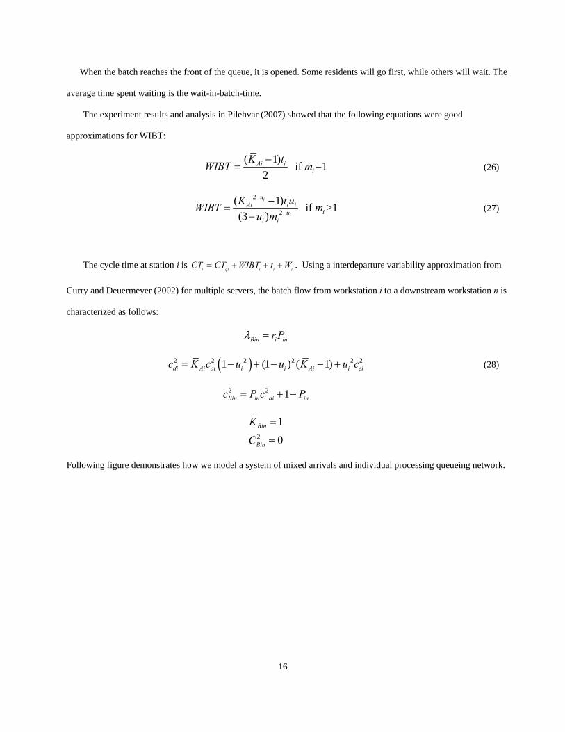
When the batch reaches the front of the queue, it is opened. Some residents will go first, while others will wait. The
average time spent waiting is the wait-in-batch-time.
The experiment results and analysis in Pilehvar (2007) showed that the following equations were good
approximations for WIBT:
( 1) if =1
2Ai i
iK tWIBT m−
= (26)
2
2
( 1) if >1(3 )
i
i
uAi i i
iui i
K t uWIBT mu m
−
−
−=
− (27)
The cycle time at station i is . Using a interdeparture variability approximation from
Curry and Deuermeyer (2002) for multiple servers, the batch flow from workstation i to a downstream workstation n is
characterized as follows:
i qi i iCT CT WIBT t W= + + + i
Bin i inr Pλ =
( )2 2 2 21 (1 ) ( 1)di Ai ai i i Ai i eic K c u u K u c= − + − − + 2 2 (28)
2 2 1Bin in di inc P c P= + −
2
1
0Bin
Bin
K
C
=
=
Following figure demonstrates how we model a system of mixed arrivals and individual processing queueing network.
16
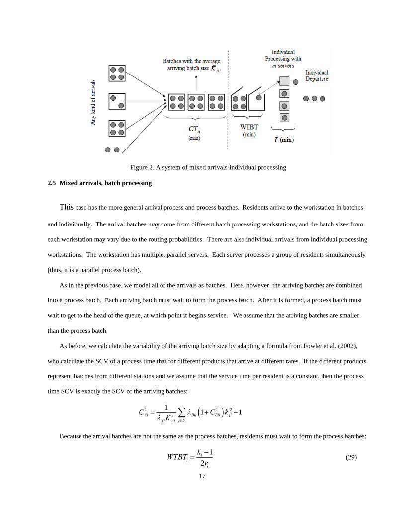
Figure 2. A system of mixed arrivals-individual processing
2.5 Mixed arrivals, batch processing
This case has the more general arrival process and process batches. Residents arrive to the workstation in batches
and individually. The arrival batches may come from different batch processing workstations, and the batch sizes from
each workstation may vary due to the routing probabilities. There are also individual arrivals from individual processing
workstations. The workstation has multiple, parallel servers. Each server processes a group of residents simultaneously
(thus, it is a parallel process batch).
As in the previous case, we model all of the arrivals as batches. Here, however, the arriving batches are combined
into a process batch. Each arriving batch must wait to form the process batch. After it is formed, a process batch must
wait to get to the head of the queue, at which point it begins service. We assume that the arriving batches are smaller
than the process batch.
As before, we calculate the variability of the arriving batch size by adapting a formula from Fowler et al. (2002),
who calculate the SCV of a process time that for different products that arrive at different rates. If the different products
represent batches from different stations and we assume that the service time per resident is a constant, then the process
time SCV is exactly the SCV of the arriving batches:
( )2 22
1 1 1i
Ai Bji Bji jij SAi Ai
C CK
λλ ∈
= +∑ 2k −
Because the arrival batches are not the same as the process batches, residents must wait to form the process batches:
1
2i
ii
kWTBTr−
= (29)
17

For the interarrival time SCV of process batches (after they are formed), we use the following result from
Pilehvar (2007):
2cbi
2 2
2
2
2 i
i
Bji Bji Bjij SAi
Aii
Bji Bjij S
cbi
K
K
cK Ck
λ
λ
∈
∈
⎛ ⎞⎜ ⎟⎜ ⎟= +⎜ ⎟⎜ ⎟⎝ ⎠
∑
∑ (30)
The arrival rate ri and AiK can be determined as discussed in output section. Then, we estimate the queueing in the
resulting G/G/m system:
2 2 12 2
2 (1 )
imbi ei i
qi i ii i
c c uCT t gm u
+ −⎛ ⎞⎛ ⎞+= ⎜ ⎟⎜ ⎟⎜ ⎟−⎝ ⎠⎝ ⎠
The queue time estimate, as suggested by Whitt (1984) and Bitran et al. (1989), includes the parameter ig , which
equals 1 if the interarrival time SCV . However, if 2 1bic ≥ 2 1bic < , then
( )( ) ( )( )22 22 1 1 / 3i bi i bi eiu c u c c
ig e− − − +
=2
Similar to individual arrival/batch service process, for the cases with the utilization higher than 90% from, waiting
time for service can be yielded by the following equation (In this type of queueing system the arrival batch rate to the
station after being formed is Ai Ai
i
Kkλ
):
2 2 2/( ) /( )
2(1 )Ai Aii bi Ai ei i Ai i i
qii
k c K c t K k mCTu
λ λ+=
− (31)
The cycle time at station i is CT . i i qi i iWTBT CT t W= + + +
The batch flow from workstation i to a downstream workstation n is characterized as follows (some of which is similar to
that in Section 2.2):
( )( )1 1 ikiBin in
i
r Pk
λ = − −
18

( )( ) ( )2
2 2 2 21 1 1 (0.2, ) 1idi i bi ei
i
uc u c Max cm
= + − − + −
(32) 2 2(1 (1 ) ) (1 )i ik kBin in di in bic P c P= − − + − 2c
( )1 1 i
i inBin k
in
k PKP
=− −
( )( )2 1 1 1 ik
in i in in inBin
i in
P k P P PC
k P− − + − −
=
The following figure demonstrates how we model a system of mixed arrivals and batch processing queueing network
where arriving batches are smaller than the process batch size.
Figure 3. A system of mixed arrivals-batch processing
2.6 Mixed arrivals, self-service
In this case, residents arrive to the workstation in batches and individually. The residents perform the process
themselves without any external resources. The cycle time at station i is i iCT t Wi= + . Moreover, to calculate for
self service station, in Equation 4 should be 1.
2cai
iw
19

To estimate the interdeparture variability we adapt the estimate used in the individual arrival, self-service case
(Section 2.3). The key change is that the interarrival variability of individuals depends upon the batch size and the batch
interarrival variability. From Curry (2002) we have the following:
( )2Interarrival variability of individuals 1Ai ai AiK c K= + − (33)
The only big assumption in the following formula is that, we assume the SCV of batch size arriving to self service
station is so small, so it’s ignorable in our calculation. That is why; we do not have any effect of 2AiC in the formula.
i ir tiρ =
From Equation 33 and Equation 20, we can obtain the following:
( )2
2 2
222 2
2 2 2 1 ei iAi ai Ai
di Ai ai Ai
Ai ai Ai ei i Ai ai Ai ei i
cK c Kc K c KK c K c K c K c
ρ2ρ ρ
⎛ ⎞+⎜ ⎟= + − +⎜ ⎟+ + + +⎝ ⎠
(34)
We should point out that that since we have individual departure from self service stations; it behaves as if we had
individual service process.
The batch flow from workstation i to a downstream workstation n is characterized as follows:
Bin i inr Pλ =
2 2 1Bin in di inc P c P= + −
2
1
0Bin
Bin
K
C
=
=
2.7 Clinic Performance Measures
The clinic capacity is determined by bounds set by each station’s capacity and the relative arrival rates:
1
1, ,min i i
i Ii i
k m rRt r=
⎧ ⎫= ⎨ ⎬
⎩ ⎭… (35)
Because of the stochastic routing, the clinic’s total cycle time is a weighted sum of the station cycle times:
20

11
1 I
i ii
TCT rCTr =
= ∑ (36)
The average number of residents in the clinic follows from Little’s Law:
1WIP r TCT= ⋅ (37)
3 EXPERIMENTAL RESULTS
In order to evaluate this queueing network approximation, we compared the model’s results to the results from
discrete-event simulation models created and run using Rockwell Software’s Arena®. To validate our formulas for our
clinic modeling (proposed six cases), we will carry out four different sets of experiments.
In all of these experiments, the first station in the clinic has a batch arrival process. The travel time between stations
is negligible in these experiments.
In the first experiment, the clinic has no self service stations, and arrival batch size is fixed. The remaining three
experiments have two tests each. In each test, the clinic has different combinations of stations and includes self service
workstations, which helps us to evaluate clinics with the different types of workstations described previously.
Additionally, these clinics have the arrival batch size variability.
For all of these experiments, we use a confidence interval of 95% for the simulation results.
3.1 Experiment One
We obtained data for this experiment from a time study of a mass smallpox vaccination clinic exercise on June 21,
2004, by the Montgomery County, Maryland, DHHS. From the exercise we collected data on the processing times at
each workstation as well as measuring how long residents spent in the clinic. The exercise, which lasted a few hours,
had hundreds of volunteers go through the clinic as residents. No residents received actual vaccinations or medications.
We constructed a simulation model and ran 10 replications of 2000 hours, with 5000 hours of warm-up time allowed
to achieve steady state. Data was recorded for mean total time and mean queueing time at each node, as well as mean
time in system and mean system WIP. The model was tested at several levels of resident arrival rates, from 20% to
97.5% of clinic capacity.
21

22
The arrival batches were always 50 residents. The batch interarrival times were exponentially distributed. Table 1
describes the eight stations in the clinic. Table 2 shows the routing probabilities from one station to another (only station
numbers are shown to save space). Table 3 lists the capacity of each station and its bound on the clinic capacity. The
vaccination station is the bottleneck station, and the clinic capacity is 5.123 residents per minute. Moreover, Table 4
shows the average total cycle time (in minutes) from the simulation results and the queueing network model in 21
scenarios in which the arrival rate increases to nearly the clinic capacity.
Table 1: Parameters for Experiment One.
Workstation Number of Staff
Mean service Time (min.)
Service Time SCV
Processing time distribution (min.)
Batch processing
size ki
1. Triage 5 0.259 0.268 0.125+EXPO(0.134) 1
2. Symptoms Room 3 1.213 0.264 0.59 + EXPO(0.623) 1
3. Holding Room 3 3.800 1.000 EXPO(3.8) 1
4. Registration 8 0.122 0.630 0.025+EXPO(0.0995) 1
5. Education 8 24.000 0.111 18+EXPO(6) 30
6. Screening 9 1.724 0.261 0.999 + GAMM(1.07, 0.678) 1
7. Consultation 6 3.770 0.308 GAMM(1.16, 3.25) 1
8. Vaccination 16 3.260 0.124 1 + GAMM(0.581, 3.89) 1
Table 2. Routing Table for Experiment One.
To
From 2 3 4 5 6 7 8 Exit 1 0.048 0.032 0.921 0 0 0 0 0 2 0 0.67 0 0 0 0 0.33 3 0.65 0 0 0 0 0.35 4 1.00 0 0 0 0 5 1.00 0 0 0 6 0.262 0.738 0 7 0.941 0.059 8 1.00

23
Table 3. Capacity for first experiment
Workstation Station capacity
(residents/min)
Relative Throughput
Bound on clinic capacity
(residents/min) 1. Triage 19.293 1.000 19.293 2. Symptoms Room 2.473 0.048 51.849 3. Holding Room 0.789 0.032 24.905 4. Registration 65.844 0.973 67.659 5. Education 10.000 0.973 10.276 6. Screening 5.219 0.973 5.363 7. Consultation 1.592 0.255 6.249 8. Vaccination 4.908 0.958 5.123
Table 4. Comparison of total cycle time for first experiment
Scenario Arrival rate to the clinic (residents/min)
Total cycle time from
simulation
Total cycle time from queueing network model
Percentage
error %
1 5.00 253.23 126.17 50.18% 2 4.85 126.85 96.25 24.13% 3 4.75 99.06 86.23 12.96% 4 4.60 79.95 76.65 4.12% 5 4.50 69.87 72.24 3.41% 6 4.25 60.51 59.32 1.97% 7 4.17 58.62 57.46 1.99% 8 3.57 48.87 49.19 0.64% 9 3.13 45.69 46.05 0.80%
10 2.78 44.48 44.59 0.26% 11 2.63 44.14 44.17 0.07% 12 2.50 44.01 43.88 0.31% 13 2.27 43.66 43.56 0.22% 14 2.00 43.83 43.51 0.73% 15 1.85 44.05 43.64 0.92% 16 1.67 44.50 44.00 1.12% 17 1.52 45.03 44.49 1.19% 18 1.43 45.56 44.86 1.53% 19 1.25 46.72 45.91 1.74% 20 1.11 47.88 47.07 1.69% 21 1.00 49.25 48.30 1.94%
Figure 4 shows the total cycle time estimates from the queueing network model and the discrete event simulation for
a variety of arrival rates. The plot for the simulation results includes error bars showing the 95% confidence interval on
each estimate.

Due to the batching at the education station, total cycle time does not always decrease as the arrival rate decreases.
At low arrival rates, there is significant waiting to form the education batches, which increases total cycle time.
When the arrival rate is low to moderate, there is a small difference between the estimates from the queueing
network model and the discrete event simulation. As the arrival rate approaches the clinic capacity, the difference
between the two estimates is large due almost entirely to different estimates for the cycle time at the vaccination station,
which has the highest utilization (since it is the clinic bottleneck).
30374451586572798693
100107114121128135142149156163170177184191198205212219226233240247254261268275282289296303310317
324331338345352359366373380
8.00
%
13.0
0%
18.0
0%
23.0
0%
28.0
0%
33.0
0%
38.0
0%
43.0
0%
48.0
0%
53.0
0%
58.0
0%
63.0
0%
68.0
0%
73.0
0%
78.0
0%
83.0
0%
88.0
0%
93.0
0%
98.0
0%
Resident arrival rate to clinic (percentage of clinic capacity)
Entit
y cy
cle
time
in c
linic
(min
)
Average of cycle time from simulation with lower and upperbound
Cycle time from formula
Figure 4. Comparison of average total cycle time for first experiment
24

25
3.2 Experiment Two
In this experiment, the clinic has seven workstations with different specifications. All of the workstations have
individual service process and the fourth station is a self service station with individual arrival.
The model was tested at several levels of resident arrival rates, from 20% to 94.5% of clinic capacity under the
different scenario. We ran 10 replications of 4000 hours, with 1000 hours of warm-up time allowed to achieve steady
state for each scenario. Data was recorded for mean total time and mean queueing time at each node, as well as mean
time in system and mean system WIP.
This experiment consisted of two tests: Test 2-1 and Test 2-2. In both tests, the average arrival batch size equals 20.
The batch interarrival times were exponentially distributed, and all of the service process distributions had gamma
distributions to allow different process time SCV. In Test 2-1, the SCV of the arrival batch size is 0.05; in Test 2-2, the
SCV of the arrival batch size is 0.2.
Table 5 describes each of the seven stations in the clinic. Note that station 4 is a self-service station. Table 6 shows
the routing probabilities from one station to another. Table 7 lists the capacity of each station and its bound on the clinic
capacity.
In this experiment, station number 7 is the bottleneck station, and the clinic capacity is 10.704 residents per minute.
We should say that in this experiment, for each test we have eight scenarios with different arrival rates.
Table 5. Parameters for clinic in Experiment Two. (Station 4 is a self-service station.)
Workstation Number St
aff
Mean service Time (min.)
Service time SCV
Processing time distribution (min.)
Batch processing size ki
1 15 1 1.11 GAMM(0.9,1.11) 1
2 9 1.752 0.52 GAMM (1.91,0.92) 1
3 8 1.154 0.40 GAMM (2.5,0.46) 1
4 n.a. 6 0.56 GAMM (1.8,3.33) 1
5 5 2 1.00 GAMM (1,2) 1
6 7 1.5 0.44 GAMM (2.25,0.67) 1
7 9 2 0.50 GAMM (2,1) 1

26
Table 6. Routing table for the clinic in Experiment Two
To From 2 3 4 5 6 7 Exit
1 0.200 0.300 0.500 0 0 0 0 2 0.400 0 0 0.600 0 0 3 0.700 0 0.000 0.300 0 4 0.250 0.350 0.400 0 5 0 0 1.00 6 0 1.00 7 1.00
Table 7. Table capacity for the clinic stations in Experiment Two
Workstation Station capacity
(residents/min)
Relative Throughput
Bound on clinic capacity
(residents/min) 1 15 1.000 15 2 5.137 0.200 25.685 3 6.932 0.380 18.243 4 n.a. 0.766 n.a. 5 2.5 0.192 13.055 6 4.667 0.388 12.024 7 4.500 0.420 10.704
Results for Test 2-1
In Test 2-1, the arrival batch size distribution is 1+Poisson (19), and the arrival batch size SCV equals 0.05. Table 8
shows the average total cycle time (in minutes) from the simulation results (Test 2-1) and from our queueing network
model. Moreover, Figure 5 shows the total cycle time estimates from the queueing network model and the discrete event
simulation for a variety of arrival rates in Test 2-1. The plot for the simulation results includes error bars showing the
95% confidence interval on each estimate.
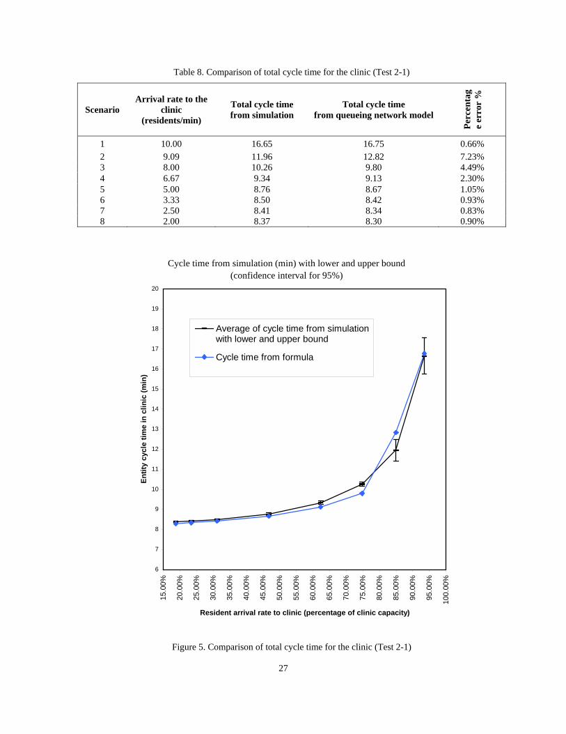
Table 8. Comparison of total cycle time for the clinic (Test 2-1)
Scenario Arrival rate to the
clinic (residents/min)
Total cycle time from simulation
Total cycle time
from queueing network model
Pe
rcen
tag
e er
ror
%
1 10.00 16.65 16.75 0.66% 2 9.09 11.96 12.82 7.23% 3 8.00 10.26 9.80 4.49% 4 6.67 9.34 9.13 2.30% 5 5.00 8.76 8.67 1.05% 6 3.33 8.50 8.42 0.93% 7 2.50 8.41 8.34 0.83% 8 2.00 8.37 8.30 0.90%
Cycle time from simulation (min) with lower and upper bound (confidence interval for 95%)
6
7
8
9
10
11
12
13
14
15
16
17
18
19
20
15.0
0%
20.0
0%
25.0
0%
30.0
0%
35.0
0%
40.0
0%
45.0
0%
50.0
0%
55.0
0%
60.0
0%
65.0
0%
70.0
0%
75.0
0%
80.0
0%
85.0
0%
90.0
0%
95.0
0%
100.
00%
Resident arrival rate to clinic (percentage of clinic capacity)
Entit
y cy
cle
time
in c
linic
(min
)
Average of cycle time from simulationwith lower and upper bound
Cycle time from formula
Figure 5. Comparison of total cycle time for the clinic (Test 2-1)
27

28
Results for Test 2-2
In Test 2-2, the arrival batch size distribution is 100-Poisson (80), and the arrival batch size SCV equals 0.2. Table 9
shows the average total cycle time (in minutes) from the simulation results and from our queueing network model.
Figure 6 shows the total cycle time estimates from the queueing network model and the discrete event simulation for a
variety of arrival rates in Test 2-2. The plot for the simulation results includes error bars showing the 95% confidence
interval on each estimate.
Table 9. Comparison of total cycle time for the clinic (Test 2-2)
Scenario Arrival rate to the
clinic (residents/min)
Total cycle time from simulation
Total cycle time from queueing network model
Pe
rcen
tag
e er
ror
%
1 10.00 18.80 18.08 3.78% 2 9.09 12.72 12.92 1.55% 3 8.00 10.71 9.86 7.90% 4 6.67 9.60 9.16 4.55% 5 5.00 8.95 8.69 2.98% 6 3.33 8.62 8.42 2.26% 7 2.50 8.51 8.34 2.03% 8 2.00 8.47 8.30 2.02%

Cycle time from simulation (min) with lower and upper bound (confidence interval for 95%)
6
7
8
9
10
11
12
13
14
15
16
17
18
19
20
15.0
0%
20.0
0%
25.0
0%
30.0
0%
35.0
0%
40.0
0%
45.0
0%
50.0
0%
55.0
0%
60.0
0%
65.0
0%
70.0
0%
75.0
0%
80.0
0%
85.0
0%
90.0
0%
95.0
0%
100.
00%
Resident arrival rate to clinic (percentage of clinic capacity)
Entit
y cy
cle
time
in c
linic
(min
)
Average of cycle time from simulationwith lower and upper bound
Cycle time from formula
Figure 6. Comparison of total cycle time for the clinic (Test 2-2)
In second test since the arrival rate is from low to moderate, there is a small difference between the estimates from
the queueing network model and the discrete event simulation.
29

30
3.3 Experiment Three
In this experiment, the clinic has seven workstations with different specifications. The first three workstations have
individual service processes. The fourth station is a self-service station. The last three stations are batch process
workstations.
The model was tested at several levels of resident arrival rates, from 39% to 97.5% of clinic capacity under the
different scenarios. We ran 10 replications of 4000 hours, with 1000 hours of warm-up time allowed to achieve steady
state for each scenario. Data was recorded for mean total time and mean queueing time at each node, as well as mean
time in system and mean system WIP.
This experiment consisted of two tests: Test 3-1 and Test 3-2. In both tests, the arrival batch size distribution is
1+Poisson (49), the average arrival batch size equals 50, and the arrival batch size SCV equals 0.02. The batch
interarrival times were exponentially distributed, and all of the service process distributions had gamma distributions to
allow different process time SCV. In Test 3-1, the process time SCV at station 4 (the self-service station) equals 0.56; in
Test 3-2, this SCV equals 1.
The routing probabilities from one station to another in this experiment are the same as second test (See Table 6).
Table 10 lists the capacity of each station and its bound on the clinic capacity which is similar for both Test 3-1 and 3-2.
In this experiment, station six is the bottleneck station, and the clinic capacity is 10.736 residents per minute.
In this experiment, each test has eight scenarios with different arrival rates.
Table 10. Table capacity for the clinic stations in the Experiment Three. (Station 4 is a self-service station.)
Workstation # Station capacity
(residents/min)
Relative Throughput
Bound on clinic capacity
(residents/min) 1 12.126 1.000 12.126 2 2.854 0.200 14.269 3 6.066 0.380 15.963 4 n.a. 0.766 n.a. 5 12.500 0.192 65.274 6 4.167 0.388 10.736 7 5.000 0.420 11.893

31
Results for Test 3-1
In Test 3-1, the process time SCV of the self service station is 0.56. Table 11 describes each of the seven stations in
the clinic for Test 3-1. Table 12 shows the average total cycle time (in minutes) from the simulation results and from our
queueing network model. Figure 7 shows the total cycle time estimates from the queueing network model and the
discrete event simulation for a variety of arrival rates in Test 3-1. The plot for the simulation results includes error bars
showing the 95% confidence interval on each estimate.
Table 11. Parameters for clinic stations (Test 3-1)
Workstation
Staf
f
Mean service Time (min.)
Service time SCV
Processing time distribution (min)
Batch process size ki
1 15 1.237 0.73 GAMM(1.38,0.9) 1 2 5 1.752 0.52 GAMM (1.91,0.92) 1 3 7 1.154 0.40 GAMM (2.5,0.46) 1 4 n.a. 6 0.56 GAMM (1.8,3.33) 1 5 1 4 0.25 GAMM (4.1) 50 6 5 24 0.01 GAMM (144,0.17) 20 7 4 24 0.01 GAMM (144,0.17) 30
Table 12. Comparison of total cycle time for the clinic (Test 3-1)
Scenario Arrival rate to the
clinic (residents/min)
Total cycle time from simulation
Total cycle time
from queueing network model
Pe
rcen
tag
e er
ror
%
1 10.42 113.12 54.41 51.90% 2 10.00 61.85 47.79 22.73% 3 9.62 49.74 45.22 9.08% 4 9.09 44.30 41.99 5.20% 5 8.70 42.14 39.64 5.93% 6 7.04 39.07 37.91 2.97% 7 5.26 39.47 38.55 2.32% 8 4.17 41.25 40.27 2.37%
Cycle time from simulation (min) with lower and upper bound (confidence interval for 95%)
30
35
40
45
50
55
60
65
70
75
80
85
90
95
100
105
110
115
120
125
130
135
140
30.0
0%
35.0
0%
40.0
0%
45.0
0%
50.0
0%
55.0
0%
60.0
0%
65.0
0%
70.0
0%
75.0
0%
80.0
0%
85.0
0%
90.0
0%
95.0
0%
100.
00%
Resident arrival rate to clinic (percentage of clinic capacity)
Entit
y cy
cle
time
in c
linic
(min
) Average of cycle time from simulationwith lower and upper bound
Cycle time from formula
Figure 7. Comparison of total cycle time for the clinic (Test 3-1)
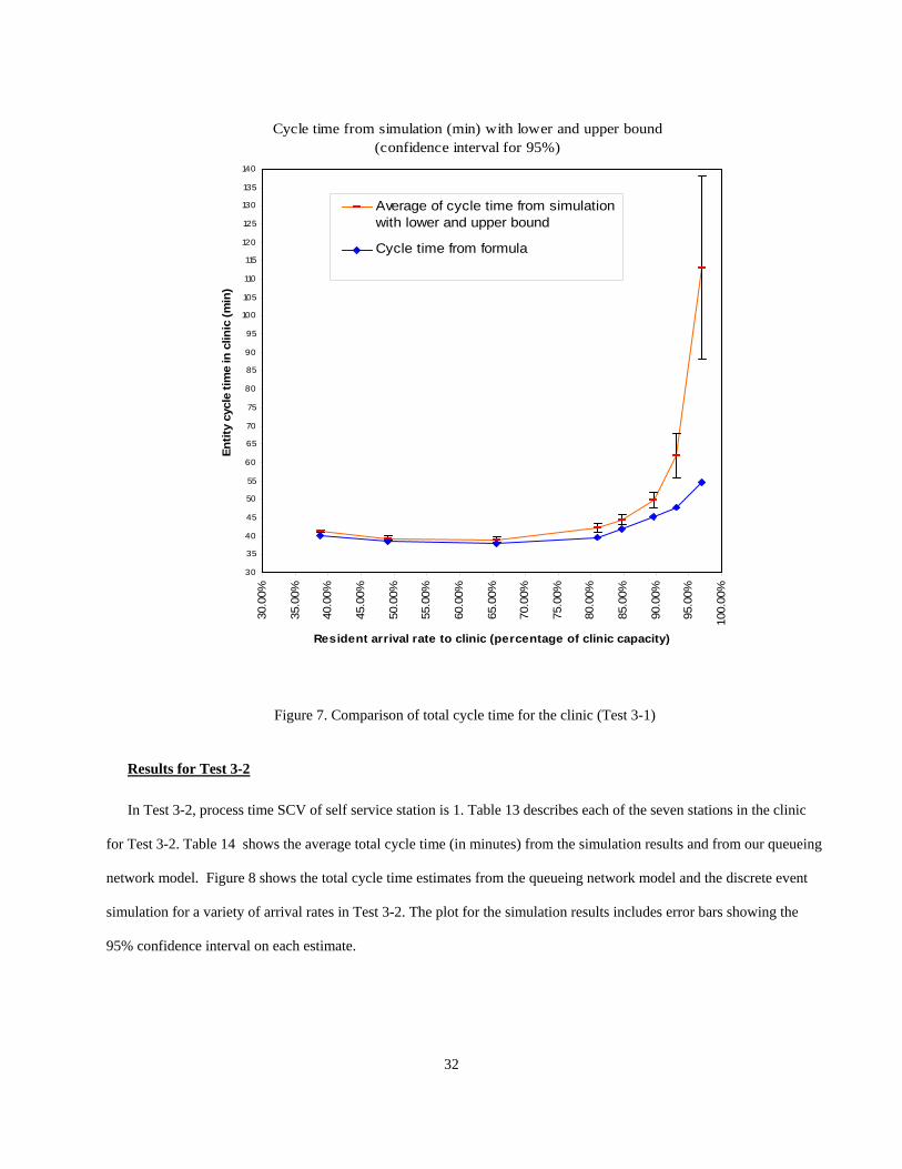
Results for Test 3-2
In Test 3-2, process time SCV of self service station is 1. Table 13 describes each of the seven stations in the clinic
for Test 3-2. Table 14 shows the average total cycle time (in minutes) from the simulation results and from our queueing
network model. Figure 8 shows the total cycle time estimates from the queueing network model and the discrete event
simulation for a variety of arrival rates in Test 3-2. The plot for the simulation results includes error bars showing the
95% confidence interval on each estimate.
32

33
Table 13. Parameters for clinic stations (Test 3-2)
Workstation
Staf
f
Mean service Time (min.)
Service time SCV
Processing time distribution (min)
Batch process size ki
1 15 1.237 0.73 GAMM(1.38,0.9) 1 2 5 1.752 0.52 GAMM (1.91,0.92) 1 3 7 1.154 0.40 GAMM (2.5,0.46) 1 4 n.a. 6 1 GAMM (1,6) 1 5 1 4 0.25 GAMM (4.1) 50 6 5 24 0.01 GAMM (144,0.17) 20 7 4 24 0.01 GAMM (144,0.17) 30
Table 14. Comparison of total cycle time for the clinic (Test 3-2)
Scenario Arrival rate to the
clinic (residents/min)
Total cycle time from simulation
Total cycle time
from queueing network model
Pe
rcen
tag
e er
ror
%
1 10.42 154.98 54.41 64.89% 2 10.00 58.45 47.77 18.27% 3 9.62 49.37 45.19 8.46% 4 9.09 44.23 41.96 5.14% 5 8.70 42.21 39.61 6.17% 6 7.04 38.93 37.86 2.72% 7 5.26 39.39 38.50 2.25% 8 4.17 41.24 40.23 2.45%

Cycle time from simulation (min) with lower and upper bound (confidence interval for 95%)
30.0035.0040.0045.0050.0055.0060.0065.0070.0075.0080.0085.0090.0095.00
100.00105.00110.00115.00
120.00125.00130.00135.00140.00145.00150.00155.00160.00165.00170.00175.00180.00185.00190.00195.00
200.00205.00210.00
30.0
0%
35.0
0%
40.0
0%
45.0
0%
50.0
0%
55.0
0%
60.0
0%
65.0
0%
70.0
0%
75.0
0%
80.0
0%
85.0
0%
90.0
0%
95.0
0%
100.
00%
Resident arrival rate to clinic (percentage of clinic capacity)
Entit
y cy
cle
time
in c
linic
(min
)
Average of cycle time from simulationwith lower and upper bound
Cycle time from formula
Figure 8. Comparison of total cycle time for the clinic (Test 3-2)
When the arrival rate is low to moderate, there is a small difference between the estimates from the queueing network
model and the discrete event simulation. As the arrival rate approaches the clinic capacity, the difference between the
two estimates is large due almost entirely to different estimates for the cycle time at station six, which has the highest
utilization (since it is the clinic bottleneck).
34
35
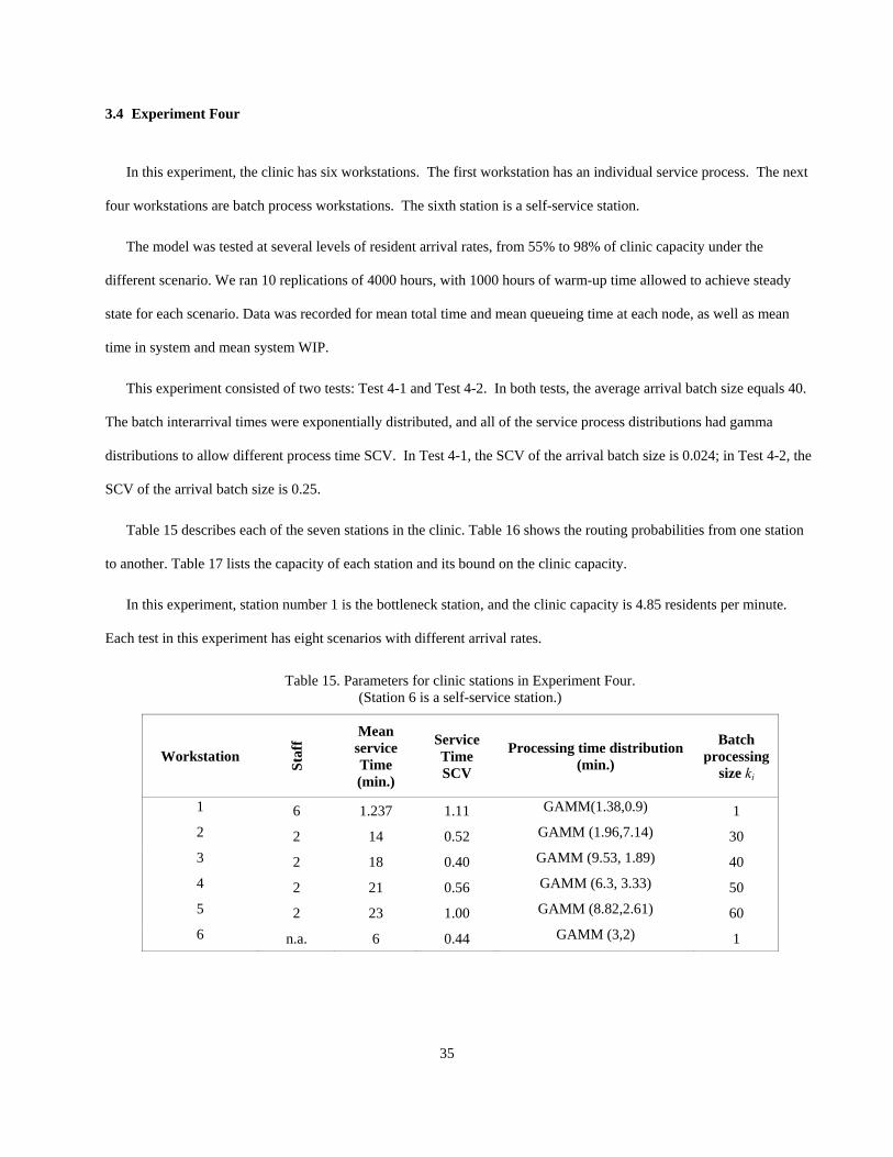
3.4 Experiment Four
In this experiment, the clinic has six workstations. The first workstation has an individual service process. The next
four workstations are batch process workstations. The sixth station is a self-service station.
The model was tested at several levels of resident arrival rates, from 55% to 98% of clinic capacity under the
different scenario. We ran 10 replications of 4000 hours, with 1000 hours of warm-up time allowed to achieve steady
state for each scenario. Data was recorded for mean total time and mean queueing time at each node, as well as mean
time in system and mean system WIP.
This experiment consisted of two tests: Test 4-1 and Test 4-2. In both tests, the average arrival batch size equals 40.
The batch interarrival times were exponentially distributed, and all of the service process distributions had gamma
distributions to allow different process time SCV. In Test 4-1, the SCV of the arrival batch size is 0.024; in Test 4-2, the
SCV of the arrival batch size is 0.25.
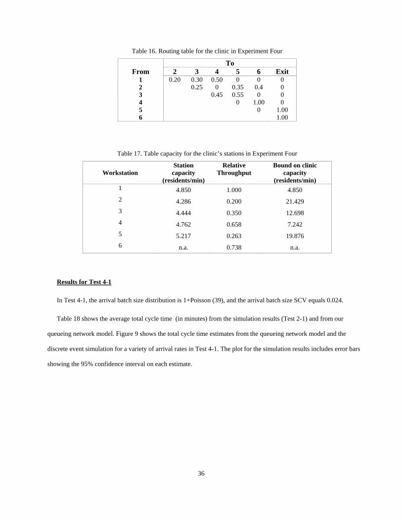
Table 15 describes each of the seven stations in the clinic. Table 16 shows the routing probabilities from one station
to another. Table 17 lists the capacity of each station and its bound on the clinic capacity.
In this experiment, station number 1 is the bottleneck station, and the clinic capacity is 4.85 residents per minute.
Each test in this experiment has eight scenarios with different arrival rates.
Table 15. Parameters for clinic stations in Experiment Four. (Station 6 is a self-service station.)
Workstation
Staf
f
Mean service Time (min.)
Service Time SCV
Processing time distribution (min.)
Batch processing
size ki
1 6 1.237 1.11 GAMM(1.38,0.9) 1 2 2 14 0.52 GAMM (1.96,7.14) 30 3 2 18 0.40 GAMM (9.53, 1.89) 40 4 2 21 0.56 GAMM (6.3, 3.33) 50 5 2 23 1.00 GAMM (8.82,2.61) 60 6 n.a. 6 0.44 GAMM (3,2) 1
36
Table 16. Routing table for the clinic in Experiment Four
To From 2 3 4 5 6 Exit
1 0.20 0.30 0.50 0 0 0 2 0.25 0 0.35 0.4 0 3 0.45 0.55 0 0 4 0 1.00 0 5 0 1.00 6 1.00
Table 17. Table capacity for the clinic’s stations in Experiment Four
Workstation Station capacity
(residents/min)
Relative Throughput
Bound on clinic capacity
(residents/min) 1 4.850 1.000 4.850 2 4.286 0.200 21.429 3 4.444 0.350 12.698 4 4.762 0.658 7.242 5 5.217 0.263 19.876 6 n.a. 0.738 n.a.
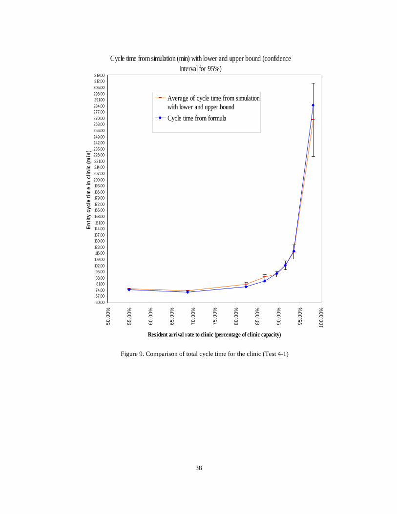
Results for Test 4-1
In Test 4-1, the arrival batch size distribution is 1+Poisson (39), and the arrival batch size SCV equals 0.024.
Table 18 shows the average total cycle time (in minutes) from the simulation results (Test 2-1) and from our
queueing network model. Figure 9 shows the total cycle time estimates from the queueing network model and the
discrete event simulation for a variety of arrival rates in Test 4-1. The plot for the simulation results includes error bars
showing the 95% confidence interval on each estimate.

37
Table 18. Comparison of total cycle time for the clinic (Test 4-1)
Scenario Arrival rate to the
clinic (residents/min)
Total cycle time from simulation
Total cycle time
from queueing network model
Pe
rcen
tag
e er
ror
%
1 4.76 268.75 285.25 6.14% 2 4.55 118.00 119.14 0.97% 3 4.44 103.04 102.64 0.38% 4 4.35 92.78 93.28 0.53% 5 4.21 89.36 85.13 4.73% 6 4.00 81.13 78.32 3.46% 7 3.33 73.69 72.40 1.75% 8 2.67 76.13 75.15 1.28%
Cycle time from simulation (min) with lower and upper bound (confidence interval for 95%)
60.0067.0074.0081.0088.0095.00
102.00109.00116.00123.00130.00137.00144.00151.00158.00165.00172.00179.00186.00193.00200.00207.00214.00221.00228.00235.00242.00249.00256.00263.00270.00277.00284.00291.00298.00305.00312.00319.00
50.0
0%
55.0
0%
60.0
0%
65.0
0%
70.0
0%
75.0
0%
80.0
0%
85.0
0%
90.0
0%
95.0
0%
100.
00%
Resident arrival rate to clinic (percentage of clinic capacity)
Entit
y cy
cle
time
in c
linic
(min
)
Average of cycle time from simulationwith lower and upper boundCycle time from formula
Figure 9. Comparison of total cycle time for the clinic (Test 4-1)
38

39
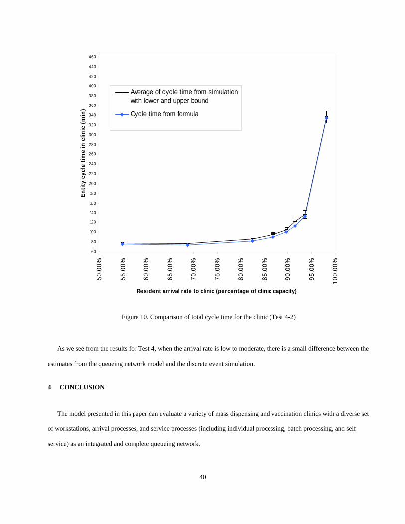
Results for Test 4-2
In Test 4-12 the arrival batch size distribution is 440-Poisson (400), and the arrival batch size SCV equals 0.25.
Table 19 shows the average total cycle time (in minutes) from the simulation results (Test 2-1) and from our
queueing network model. Figure 10 shows the total cycle time estimates from the queueing network model and the
discrete event simulation for a variety of arrival rates in Test 4-2.
Table 19. Comparison of total cycle time for the clinic (Test 4-2)
Scenario Arrival rate to the
clinic (residents/min)
Total cycle time from simulation
Total cycle time
from queueing network model
Pe
rcen
tag
e er
ror
%
1 4.76 336.60 334.52 0.62% 2 4.55 135.95 132.27 2.70% 3 4.44 122.05 112.11 8.15% 4 4.35 105.20 100.62 4.35% 5 4.21 95.39 90.57 5.05% 6 4.00 85.59 82.04 4.14% 7 3.33 76.84 73.90 3.82% 8 2.67 78.14 75.84 2.94%
60
80
100
120
140
160
180
200
220
240
260
280
300
320
340
360
380
400
420
440
460
50.0
0%
55.0
0%
60.0
0%
65.0
0%
70.0
0%
75.0
0%
80.0
0%
85.0
0%
90.0
0%
95.0
0%
100.
00%
Resident arrival rate to clinic (percentage of clinic capacity)
Entit
y cy
cle
time
in c
linic
(min
) Average of cycle time from simulationwith lower and upper bound
Cycle time from formula
Figure 10. Comparison of total cycle time for the clinic (Test 4-2)
As we see from the results for Test 4, when the arrival rate is low to moderate, there is a small difference between the
estimates from the queueing network model and the discrete event simulation.
4 CONCLUSION
The model presented in this paper can evaluate a variety of mass dispensing and vaccination clinics with a diverse set
of workstations, arrival processes, and service processes (including individual processing, batch processing, and self
service) as an integrated and complete queueing network.
40

41
The model synthesizes a variety of existing and new proposed models into a systematic approach and includes
significant and innovative contributions. One of the components is a model of a queueing system with variable arrival
batches and a batch service process whose batch size is larger than the arrival batch. Another innovative component is a
model that describes the departure process of self-service workstations.
This model is not limited to just one mass dispensing and vaccination clinic. The model takes into account arrival
batches, process batches, parallel servers, stochastic routings, and self-service stations. The model provides good
estimates for total cycle time in a typical mass dispensing and vaccination clinic scenario when resident arrival rates are
low or moderate (less than 85% of capacity). Compared to results from a discrete event simulation model, the total cycle
time estimates have an error of less than 8%. As arrival rates approach clinic capacity, the error in the total cycle time
estimates is small in some cases but increases in others. It is not clear why the model performance varies in this way.
Despite the discrepancies that can occur in some scenarios, we believe that this model is an important contribution.
We are aware of no other open queueing network approximations that can model such a wide range of processes. Thus,
the approximations presented above, combined systematically in this way, represent a significant step towards a
comprehensive model for open queueing networks. We continue testing to evaluate the approximations’ accuracy for
other types of clinics and are implementing the approximations in software for generating clinic planning models.
Although planning mass dispensing and vaccination clinics motivated the development of this queueing network
approximation, we expect that the model will be useful in other applications where the queueing networks have similar
characteristics. Testing using data relevant to these applications should be done to determine the accuracy of the
approximations.
REFERENCES
Aaby, K., Herrmann, J.W., Jordan, C., Treadwell, M., and Wood, K. (2005) Improving Mass Vaccination Clinic
Operations, Proceedings of the International Conference on Health Sciences Simulation, New Orleans, Louisiana,
January 23-27, 2005.
Aaby, K., Herrmann, J.W., Jordan, C., Treadwell, M., and Wood, K. (2006a) Using Operations Research to Improve
Mass Dispensing and Vaccination Clinic Planning, Interfaces, Volume 36, Number 6, pages 569-579.
42
Aaby, K., Abbey, R., Herrmann, J.W., Treadwell, M., Jordan, C., and Wood, K. (2006b) Embracing Computer Modeling
to Address Pandemic Influenza in the 21st Century, Journal of Public Health Management and Practice, 12(4) 365-
372.
Buzacott, J.A., Shanthikumar, J.G. (1993) Stochastic Models of Manufacturing Systems. Prentice Hall, Englewood
Cliffs, N.J.
Curry, G.L., Deuermeyer, L.B. (2002) Renewal approximations for the departure processes of batch systems, IIE
Transactions, 34, 95-104.
Fowler, J.W., Phojanamongkolkij, N., Cochran, J.K., Montgomery, D.C. (2002) Optimal batching in a wafer fabrication
facility using a multi-product G/G/c model with batch processing, International Journal of Production Research,
40(2) 275-292.
Gross, D., and Harris, C. (1974) Fundamentals of Queueing Theory. John Wiley and Sons, New York.
Hall, R.W. (1991) Queueing Methods for Services and Manufacturing, Prentice Hall, Englewood Cliffs, New Jersey.
Herrmann, J.W. (2008) Disseminating Emergency Preparedness Planning Models as Automatically Generated Custom
Spreadsheets, to appear in Interfaces.
Hopp, W.J., and Spearman, M.L. (2001) Factory Physics: Foundations of Manufacturing Management, Second Edition,
Irwin/McGraw-Hill, New York.
Hu, M.-D., and Chang, S.-C. (1998) Translating output specifications to production flow requirements for re-entrant
lines, Proceedings of the 37th IEEE Conference on Decision and Control, Tampa, Florida, December 16-18, 1998,
Volume 2, 2160-2165.
Kamath, M., Sivaramakrishnan, S., and Shirhatti, G. (1995) RAQS: A software package to support instruction and
research in queueing systems, 4th Industrial Engineering Research Conference Proceedings, IIE, Norcross, Georgia,
pp. 944-953.
Kaplan, E.H., Craft, D.L., Wein, L.M. (2002) Emergency response to a smallpox attack: The case for mass vaccination,
Proceedings of the National Academy of Sciences, 99(16), 10935-10940.
Pilehvar, A. (2007) Queueing Network Approximations for Mass Dispensing and Vaccination Clinics, M.S. Thesis,
University of Maryland, College Park.
Pilehvar, A., and Herrmann, J.W. (2008) Approximating the Departure Variability of Self-Service Stations, working
paper, Institute for Systems Research, University of Maryland, College Park, Maryland.
43
Segal, M. and Whitt, W. (1989) A queueing network analyzer for manufacturing. Proceedings of the 12th International
Teletraffic Congress, Torino, Italy, June 1988, 1146-1152.
Shore, H. (1988) Simple approximations for the GI/G/c queue - I: steady state probabilities, Journal of the Operational
Research Society, 39(3), 279-284.
Treadwell, M. (2006) Queueing Models and Assessment Tools for Improving Mass Dispensing and Vaccination Clinic
Planning, M.S. Thesis, University of Maryland, College Park.
Whitt, W. (1983) The queueing network analyzer. Bell Systems Technical Journal, 62, 2779-2815.
Whitt, W. (1984) Approximation for the departure and queues in series. AT&T Laboratories, Holmdel, New Jersey.
ACKNOWLEDGMENTS
The authors wish to thank Mark Treadwell for his work on an earlier version of this model and the staff of Montgomery
County (Maryland) Public Health Services, particularly Kay Aaby and Rachel Abbey, for their assistance. This
publication was supported by Cooperative Agreement Number U50/CCU302718 from the CDC to NACCHO. Its
contents are solely the responsibility of the University of Maryland and the Advanced Practice Center for Public Health
Emergency Preparedness and Response of Montgomery County, Maryland, and do not necessarily represent the official
views of CDC or NACCHO.
AUTHOR BIOGRAPHIES
ALI PILEHVAR is a Ph.D. student in the Robert H. Smith School of Business at the University of Maryland, College
Park. His e-mail address is <[email protected]>.
JEFFREY W. HERRMANN is an associate professor at the University of Maryland, College Park, where he holds a
joint appointment with the Department of Mechanical Engineering and the Institute for Systems Research. He is the
director of the Computer Integrated Manufacturing Laboratory. He is a senior member of IIE and also a member of
INFORMS, ASME, SME, and ASEE. He received his Ph.D. in industrial and systems engineering from the University
of Florida. His e-mail address is <[email protected]>.