Embed Size (px)
Citation preview

J . Fluid Mech. (1981). vol. 102, pp. 141-167
Printed in Great Britain
141
The instability of the ocean to Langmuir circulations
By S. LEIBOVICH AND S. PAOLUCCIT Sibley School of Mechanical and Aerospace Engineering, Cornell University,
Ithaca, New York 14853
(Received 3 August 1979 and in revised form 13 March 1980)
It has been proposed that Langmuir circulations arise as an inshbility of the equations describing the Eulerian-mean flow in bodies of water supporting surface waves and subject to an applied wind stress. In infinitely deep density-stratified water, the solution of an appropriate initial-value problem is a unidirectional, time-dependent current. The stability of this current to two-dimensional (roll) disturbances is investi- gated by an energy analysis and by linear theory. It is found that the energy stability estimates and linear stability limits are very close, showing that subcritical instability, if it occurs, is limited to a very narrow region in parameter space. According to the present results, conditions typically occurring in the ocean are highly unstable to the Langmuir circulation instability.
1. Introduction A theory of wind-driven convective motions in the upper layers of lakes and the
ocean, discovered by Langmuir (1938) and named after him, has been offered by Craik & Leibovich (1976). This theory has been extended, refined, and its consequences explored by Leibovich (1977a), Leibovich & Radhakrishnan (1977), Craik (1977) and Leibovich (19773).
The theory rests upon a set of equations, given in its most complete form in Leibovich (19773) andLeibovich (1980) and which we will generically call the CL model, for the Eulerian-mean flow in an ocean subject to surface wave activity and an applied wind stress. These equations permit solutions with rectilinear currents that are functions only of depth and (possibly) time. Craik (1977) showed that these solutions are un- stable in water of constant density, and Leibovich (19773) subsequently showed that they are unstable in water with a stable density stratification providing the wind stress exceeded a minimum value. The currents analysed in these papers, however, were not those that develop from the CL equations, and viscosity and heat transfer are ignored in both papers except by reference to an analogy of unknown utility.
Leibovich & Paolucci (1980), referred to as LP henceforth, have examined this instability mechanism by direct numerical solution of the initial-value problem for the fully nonlinear CL equations. An infinitely deep ocean is assumed to be at rest and to have a constant (statically stable) temperature gradient for time t < 0. At t = 0, tt constant wind stress and surface wave activity are imposed, and the evolution of the Eulerian-mean motion is traced. For small time, the motion is identical with that of the stress Rayleigh problem and there is no change of temperature, but this xolution is unstable to small disturbances and strong convective activity takes place.
t Prerscnt addrcsv : Sandia National Laboratories, Livormore, California 94550.
0022-1 120/81/4679-2740 $02.00 Q 1981 Camhritlgo University Press

142 S. Leibovich and S. Pmlucci
Since the motion is assumed independent of the co-ordinate in the wind direction, the instability takes the form of rolls and a mixed layer and thermocline develop. As time proceeds, the length scale and strength of the rolls increase, and there seems to be an energy cascade from small to large scales.
In this paper, we establish global stability bounds and linear instability limits for the unidirectional solution of the CL equations; thus we deal with the problem studied by LP, but under conditions near marginal instability. The present paper concerns only stability to two-dimensional disturbances. We have also examined the global stability question for three-dimensional disturbances, and shall report on that work (which poses a more difficult computational problem) elsewhere. The principal out- come, however, is the inference that the unidirectional current is most unstable to two-dimensional rolls with axes aligned with the wind. This is just what is observed in the ocean and implies that the stability results given in this paper are the relevant ones.
Two complications seldom dealt with in stability theory are simultaneously present in this problem: (a) the motion whose stability we study takes place in an infinite domain, and ( b ) it is unsteady. The first complication poses problems for the energy stability theory that have already been faced by Dudis & Davis (1971a, b ) , and we follow t'heir lead. Optimal global stability bounds are found by a Galerkin approxima- tion to the solution of the associated variational problem.
The second complication, the unsteadiness of the basic flow, implies that the linear stability problem is non-separable. We reduce the problem to a system of ordinary differential equations in time for the coefficients in a Galeikin approximation to the solution. In contrast to some unsteady base flows, precise stability limits can be given by what amounts to a quasi-steady (algebraic) analysis. A referee has brought to our attention the interesting work by Homsy (1973), Gumerman & Homsy (1976) and Wankat & Homsy (1977) in which rigorous lower bounds for the onset of instability have been obtained for unsteady flows in bounded domains using energy stability theory. In the present paper, upper bounds for the onset time (suitably interpreted) for unstable flows are established using linear theory. Our interest here is mainly to show that the onset time is short; and we in fact do find the upper bounds for onset time are small.
Since the motion takes place in an infinite domain, a continuous as well as a discrete spectrum is expected for the linear stability problem. The Galerkin approximation yields only a discrete spectrum since i t has finite dimension, but the development of the continuous spectrum is indicated by the increase in eigenvalue density as the order of the Galerkin approximation is increased.
Two dimensionless parameters control this problem : the Langmuir number, La, which is an inverse Reynolds number based upon wind stress and surface wave para- meters; and a Richardson-number-like parameter Ri that provides a measure of the (stabilizing) density stratification in the basic flow. Ranges of these parameters that are physically significant for the ocean turn out to be highly unstable according to the present analyses.
We find that the global stability bound and linear instability criterion almost coincide. For homogeneous water (Ri = 0), for example, stability is guaranteed for La > 0.68 and instability occurs for La c 0.66. Thus we can almost characterize the stability of this flow completely; the only unanswered question is a possible

Instability of the ocean to Langmuir circulations 143
subcritical instability in the gap 0.66 < La < 0.68. Similar results, but with a slightly larger gap, hold for cases with Ri # 0.
We should add, a t this point, further comment about our choice of thestressRayleigh problem as the (mean) current whose stability is examined. Certainly it is exceptional to initiate motion in the ocean by the imposition of a wind stress over quiescent water, as this basic flow contemplates. Furthermore, it is possible that the time evolution of the surfaoe wave field, which is ignored in this farmulation, that is engendered by the applied wind stress could introduce effects comparable in importance to the time evolution of the current which is emphasized in this paper. More general situations can be treated using the formulations in this paper, We believe, however, that the problem addressed here, although highly idealized, is fundamental for a number of reasons. The destabilizing factors for Langmuir circulations, wind and waves, are introduced at the surface, and the instability works its way down from the top. Thus, imagine a current that is more or less uniform and unidirectional from the surface to the base of the mixed layer (this is a model often taken for the current in the ocean mixed layer), to exist prior to the imposition of a wind stress, or to a shift in wind direction. In fact, if the shear in this current is concentrated a t the base of the mixed layer, then, by a Galilean transformation, we may move with the current, so that we see a quiescent upper layer overlying water moving a t (essentially) constant speed. When the wind stress is imposed, one can expect the surface waters to respond initially as if the mixed layer were infinitely deep, with the surface stress transmitted to the water through a shear layer resembling the Rayleigh stress layer. I f this layer is un- stable, and if the instability develops sufficiently rapidly (and from the theory it seems to do so) then for some time the bottom of the pre-existing mixed layer will not greatly affect the motion, including any associated instabilities, near the surface.
The problem of time evolution of the surface wave field is one that we are unable to address a t this stage; the growth of wind waves is a notoriously difficult subject, and it does not seem to us that its theory is sufficiently advanced to establish the kind of information needed to introduce wave growth into a theory of Langmuir circulation. Again, however, despite the role it may play in the ocean, the present formulation seems to us to be fundamental. As shown by Faller & Caponi (1978) and by Faller (1978), Langmuir circulations can be produced by mechanically generated waves, upon which a wind stress is suddenly imposed. Since the circulations form a t very short fetches, it seems unlikely that the growth of waves by wind plays much of a role in these laboratory experiments.
A final reason for our choice of basic flow state is our desire to complete the investi- gation begun by LP, who showed that Langmuir circulations, beginning from the basic state considered here under highly supercritical conditions, develop current and temperature fields resembling ‘real ’ mixed layers. The direct numerical simulation used in LP is, however, not a feasible method of determining the requirements for instability; stability analyses, such as those described here, are more useful.
2. Governing equations The equations governing the Eulerian means for a fluid under the action of surface
waves and satisfying the Boussinesq approximation are given by Leibovich (1977b, equation ( 12)). Let the mean free surface coincide with the (x, y) plann, let, t,he wind

144 S . Leibovich and S . Paolucci
stress be directed along the positive x axis (unit vector i ) , and let z be measured vertic- ally upwards (unit vector k) from the mean free surface. It is assumed that the ocean is infinitely deep and initially at rest with a linearly increasing temperature T'(z). A t time t = 0, a mind stress p u i (where u* is the water friction velocity and p a reference water density) and surface waves with characteristic frequency u, wavenumber K,
and amplitude a are imposed. We will deal here only with motions and disturbances that are independent of x,
and make all quantities dimensionless following Leibovich ( 1 9 7 7 ~ ) . In particular, we refer all lengths to K-1, time to ( v T / ~ ) * a - 1 ~ - 1 u ; ' , modified pressure n to ~ % : u v , ~ , x-directed velocity component to u i v ~ l K - ~ , y and z velocity components to u* sub$, and temperature deviation from the constant gradient conduction solution to r 1 T r . Here V~ is an (assumed constant) eddy viscosity representing turbulent diffusivity of momentum.
The presence of surface waves implies the existence of a second-order (in wave slope c = a K ) Stokes drift. This Stokes drift, velocity us, through the 'vortex force' us x o generated by us and the mean-flow vorticity o, is the only effect of the averaging to cause the equations to differ in form from those for instantaneous Eulerian quantities. We make the Stokes drift dimensionless by referring it to a 2 K u . We allow the Stokes drift to depend only upon depth, and to be in the x direction. Later, for specific results, me will take the dimensionless Stokes drift to be
us -- U&)i = 2e2*i. (1)
This form is appropriate to infinitesimal monochromatic irrotational water waves, but the specific form chosen for us will make little difference in our results.
With t,hese scaling choices and assumptions on u, made, the dimensionless governing equations may be written in the form
Pa)
( 2 b )
v . v = 0, ( 2 4
av at
ae -+v.VO = -k.v+LaPr-lV28, at
--+v.Vv = U,Vu+RiOk-Vn+LaV2v,
where v is the dimensionless Eulerian-mean velocity vector, and 8 is the dimensionless temperalme deviation from the conduction solution, La is the Langmuir number introduced by Leibovich (1 9 7 7 ~ )
t La=- ( : ) KVT , au*
and Pr b a (turbulent) Prandtl number
P r = vT /aT ,
where aT is the (eddy) diffusivity of heat. The parameter Ri is

Instability of the ocean to Langmuir circulations 145
the denominator is a measure of the squared velocity gradient in the plane perpen- dicular to the wind; thus this number plays the role of an overall Richardson number (which is what we shall call it).
We are interested in an initial-value problem in which a stress is applied to the plane z = 0 at time t = 0, and this leads to the following (dimensionless) initial and boundary conditions on the velocity vector:
V(X)O) = 0, ( 3 a )
v ( x , t ) + O as z + -XI forall t <XI, ( 3 b )
( 3 c ) a - ( k x V ) = ( O , H ( t ) , O ) , k . v = O at z = O , az
where H ( t ) is the Heaviside unit function (H = 0 for t < 0, H = 1 for t 3 0). A variety of thermal boundary conditions could be imposed, corresponding to wide
range of physically relevant problems. In this paper, we assume isothermal conditions at z = 0, and therefore take
e(x,o) = 0, ( 3 d )
e = o at z = o , ( 3 4
e + o as Z + - C O . (3.f 1
A solution to problem (2)) ( 3 ) is a developing unidirectional current corresponding to the stress Rayleigh problem (see Leibovich 1 9 7 7 ~ ) equations (23 ) ) ( 2 4 ) ) :
z ?I=-- 2(tLa)4 *
We wish to study the stability of the system (4). If we introduce perturbations to (4) by substituting
(5) v = v + U , e = is+$ = 4) 7T = ? i f p ,
into ( 2 ) ) noting that the barred quantities themselves satisfy (2)) the results are the following equations for perturbation quantities
aU %+ u. V u = U,Vu - wDUi+ Bi$k - V p + LaV2u, (Gal

146
with auxiliary conditions
S. Leibovich and S. Paolucci
k . u = D ( u x k ) = $ = O on z = O , ( 7 4
u+O, $ - + O as z+--oo, ( 7 b )
U(X,O) = uo(x), $(x, 0) = 0, ( 7 c )
where uo(x) is solenoidal and satisfies ( 7 a , b ) . We have denoted (x, y, x ) components of the perturbation velocit,y vector u = (u, w, w).
3. Energy analysis Energy stability analyses typically proceed by forming the time rate of change of
a positive definite functional of perturbation quantities in a given volume of fluid and then establishing conditions under which this must decrease in time for arbitrary disturbances. The volume is usually selected by requiring periodicity of perturbations in one or more directions. We shall require all perturbations to satisfy ( 7 ) and to be periodic with wavenumber k (or Fourier transformable) in the cross-wind direction y. The volume of integration V is taken to be a unit distance in the x direction, the interval 0 < y < 27r/k (or IyI < co if the disturbances are Fourier transformable), and the entire depth of the fluid -a < z < 0.
The construction of the most straightforward energy functional begins by taking the scalar product of (6a ) and u, and integrating over V . Since u is solenoidal, use of the divergence theorem and ( 7 ) eliminates the scalar p , and an equation for the per- turbation kinetic energy results. Similar manipulation with the equation for thermal energy yields an equation for the conservation of squared perturbation temperature. A linear combination of these two equations, linked by a positive coupling parameter, can be used to develop an optimized energy stability estimate, following Joseph (1976b). In the present case, disturbances are assumed independent of x, and this introduces additional flexibility that permits the final results to be further optimized. Thus, me proceed slightly differently. Let
u = ui+w,
where w = vj +wk is the projection of u onto the y, z plane. Integrating the scalar product of w with (Ga) over V , and applying the divergence theorem and boundary conditions gives
+uwDU,-RiwQ+LaVw:Vw dx = 0. 1 The scaler product of ( 6 a ) with ui, when manipulated in the same way, yields
while the product of ( 6 b ) with $ yields

Instability of the ocean to Langmuir circulations 147
Multiplying (10) by u2Ri, ( 9 ) by u,, and adding the resulting expressions to (8) gives
dE - = I -LaD, at
where the energy functional
E = - ( w . w + a l u 2 + ~ 2 R i $ 2 ) d x k f V
is positive for all perturbations for positive choices of the assignable coupling para- meters a1 and u2 (recall that we only consider positive, or stabilizing, values of Ri). In (1 I), D is the (positive definite) dissipation functional
D =Iv (Vw:Vw+a,lVu12+a2RiPr-1JVq5J2)dx, (12)
and I is the energy production functional
I = - Iv [uwDo+ Ri(cr,- 1)wq5]dx.
In I, we have introduced the symbol 0, 0 = u,+a,u.
The first energy stability analysis in an unbounded domain seems to have been that of Dudis & Davis (1971a), who note that apriori estimates customarily used to bound the production integral by the dissipation integral fails in unbounded flow. This precludes the analysis leading to the exponential decay of disturbances when global stability criteria are met. They nevertheless establish that the dissipation integral, D, vanishes as t + CQ. Since all perturbations in their problem vanish on a plane (say z = 0), they are able to conclude from D + 0 that the energy in a slab of fluid of any bounded thickness extending from z = 0 must vanish as t --f 00. This is weaker than asymptotic stability in the mean.
From ( l i ) ,
dt
and, upon integration,
Z(t) -E(O) = -La D(7) [ 1 - La-lD-lI] d7. so’ Suppose
I La,(t) = max-
D
exists for all t , where the maximum is taken over a suitable class of functions to be described later, and let
where 0 < Laa < La, (15)
Ln, = max Ln,(t). 1

148 s. Leibovich and 8. Paolucci
Then the int,egrand in (14) is positive for all t ; since E( t ) must also be positive, (14) shows t.hat
Assuming E(0) < co, D dt c co, and so D +- 0 as t + 00, as found by Dudis & Davis l o * (1971a) using essentially this argument. Furthermore, E(t) < E(0) for all t if (15) holds, which proves simple stability.
In the present problem, u does not vanish on x = 0, and we cannot invoke the a priori bounds which allow Dudis & Davis (1971 a) to infer from the result D +- 0 that the energy in finite subdomains must vanish as t --f 00. We can show that the Dudis & Davis stability holds, nevertheless, by using a different argument. Consider a finite volume B between the planes z = -dl and z = 0, and between y = y, and y = yl+d,, where d,, y1 and d, are arbitrary, but finite. Let
0 < b < D, b + 0 as t + 00 whenever (15) holds. Thus u + ti+u*, where ti is a, constant vector, and u* = O ( b i ) as b + 0. Thus
where
and
But
E = +lii)2dld2+E*,
1 E* = 5 . u* dx + 5j7 u * ~ dx
E * = O ( b 4 ) as b + O .
B(t) < E(t ) < E(O),
when (15) holds and, since d, and d, are arbitrary, this inequality is eventually violated unless ]ti/ = 0.
We note that Galdi & Rionero (1977) rigorously show, for problems like ours, that (15) does imply asymptotic stability in the mean in unbounded domains for all per- turbations satisfying a certain equi-absolute continuity condition. Unfortunately, there is no way to decide a priori that perturbations governed by (6) and (7) and evolving from physically reasonable initial conditions will in fact satisfy their technical condition.
We now turn to the maximum problem for La, and La,. This problem is guaranteed to have a solution (Galdi & Rionero 1977) provided an integrability condition on the rate of strain of the basic flow is met. It is easily verified that this is the case in the present problem; since we will actually find the solution to the maximum problem, there is no need to display the verification.
Thus we seek T

Instability of the ocean to Langmuir circulations 149
where the maximum is sought in the class of functions 9' with u solenoidal, which yield finite values of the functional E , and which satisfy the boundary conditions ( 7 ) and (if applicable) the periodicity conditions satisfied at each instant by the physical perturbations .
The maximum of I / D depends parametrically on time, as well as vl, v2, Ri, Pr. We shall let
(17) 1
La, =
and define 1
max min A La, = min max La, = u,,u*>o 1
u,,u,>o 1
where the extrema are taken over all possible non-negative values of t, bl and v2, with Ri and Pr held fixed. If a finite La, exists, then global monotonic stability is assured if
and this criterion is optimal. The variational problem (16) for La,, or alternatively for h(t) (we suppress the other
parameters upon which h depends when no confusion will result), is associated with the following Euler equations (here we use appendix B 2 of Joseph 1 9 7 6 ~ ) :
La > La, (19)
V ~ U = - h wDO, 201
V2w = &I[(uDO+Ri(a,- l)$)k+Vp], (20b) h Pr
v29 =20-,(v2-1)w,
v.w = 0, w = (O,v,w), P o d 1 where p is a function that can be regarded as maintaining the solenoidal character of w.
The case v2 = 1 is particularly simple, since in that case the temperature-like variable 9 does not influence the stability criterion; there is, to our knowledge, no physical explanation for the decoupling nor does it generally lead to the best results.
Since all functions are assumed independent of x and the coefficients of (20) are independent of y, we may seek a solution in the form
(21 1 (u, v, W , P , 9, = (@.w, w, W ) , 4(4, &)) eSkV.
The variable p can be eliminated by taking the curl of (20b); if this is done, and ( 2 1 ) inserted into the result, ( 2 0 ) reduces to the set of ordinary differential equations
h (D2-k2)24 = -,k2[&DU+Ri(a,- I ) $ ] ,

150 8. Leibovich and 8. Paolucci
with boundary conditions
For a given value of t and k, let the smallest positive eigenvalue h of the system (22) be X(t; k). For fixed t , X( t ; k) = X(t ; - k) so it is sufficient to consider only positive values of k; we obtain a solution to the maximum problem by seeking the minimum of X over all t 2 0 and k 2 0. The optimal result is found by maximizing this minimum X over all possible values of crl and u2.
It is convenient for numerical purposes to transform (22) by setting 6 = eg, thus placing the problem in a finite domain in 5. The eigenvalue problem becomes
l h
2 u1 ( 2 3 4 ( L - P ) Q = --(DO)@,
(L-k2)2@ = -*hk2[QDO+Ri(a2- 1)$], (23b)
42 = 8 = $ = 0, and all derivatives bounded, on 6 = 0, (23e)
and we now regard 0 to be given as a function of 6. To solve this problem, we employ the Galerkin technique and expand &,a, and 4 in
linearly independent, complete sets of functions ui, wi and g5i satisfying the boundary conditions (23d, e),
Here the bi are constants that will be chosen to satisfy the differential equations (23 a-c) .
Upon substituting (24) into (23), we get
The functions Rj, which depend explicitly on the coefficients bi and position c, are the residuals which result because (24) is not a solution of (23). In the Galerkin method,

Instability of the ocean to Langmuir circulations 151
equations for the coefficients bi are obtained by requiring the residuals to be orthogonal to each of the approximating functions (Finlayson 1972),
(Rlu,) = {R2wj) = (R3q5*) = 0, j = 1 , 2 , ..., N ,
where we use the notation
This leads to a system of 3 N linear, homogeneous algebraic equations for the bi, which can be written in the form
The matrices 3Er and #are 3Erb = A$,. ( 25 )
3Er = ( 1 i2 t), where the K,, K,, K3 and zero entries are all N x N matrix blocks, with
and
where again each entry is an N x N matrix, and
A non-zero solution of (25 ) exists if and only if the determinant of coefficients vanishes,
det(Sf-A%) = 0. (27 )
Equation ( 2 7 ) is a 3Nth-order polynomial equation. Thus, an N-term Galerkin expan- sion produces the first 3N among the infinite number of eigenvelues of the system (23 ) .
The condition (18) requires only the smallest positive value of A, which must be minimized over all positive values oft and k, and then maximized over all cl, v2 > 0. For any Richardson number, 6, and g2, the numerical values for 8 fixed t and for different k for the first as well as higher approximations can be obtained once the basis functions ui, w i and #i, and an appropriate form for the Stokes drift, are chosen.

153 S. Leibovich and 8. Paolucci
N 1 5 G 7 8 9
10 11 12 13
4 5.87883 2.77153 2-67 102 2.61187 2.55758 2.52125 2.48707 2.46223 2.43845 2.42022
Cliange (%)
- 3.63 2.22 2.07 1-42 1.36 1 *oo 0.97 0.75
TARLE 1. Convergence of the minimum positive eigenvalue at k = v1 = u2 = 1 for the global stability problem as t + co.
To be consistent with our previous numerical work (LP) we take the turbulent Prandtl number to be Pr = 6.7, and (1) for the Stokes drift. We also adopt the basis functions
Ui(5) = (5- QC2) (1 - 5)2i-2, ( 2 8 4
Wi(5) = (55- 352) (1 - 5p-1, (28b)
@dC) = 5i(l - 5 Y s ( 2 8 4
which satisfy the boundary conditions (23d, e). The choices (28) are probably not the most efficient for computational purposes, but they are easy to construct, and seem adequate for our purposes. The eigenvalue problem (25) was solved with a standard International Mathematical and Statistical Library (IMSL) eigenvalue subroutine for a real non-symmetric matrix system. For each fixed t , the minimum positive A for all k's can be found. Repetition of the numerical experiment for all values oft yields the minimum positive h for all k's and for all t ; this furnishes an estimate of La,. This estimate can be improved by forming a table for the values of the minimum positive A as u1 and u2 are varied. The optimizing parameters for Ri = 0, are u1 = 0.25, and u2 = 1.0 and yield h = 1.46 at k = 0.32 and t = co. The optimizing parameters for Ri = 0.1 and Ri = 0.25 were also found and will be summarized in $4. In all cases min h is obtained at t = co.
t
We considered the accuracy provided by the N = 13 Galerkin expansion to be adequate for our purposes. Convergence of the minimum positive h with increasing N is monotonic, and is demonstrated in table 1 for the case 6, = 1, r2 = 1 and k = 1 (which is a case with a typical convergence rate). Further comment,s on accuracy may be found in the appendix.
4. Instability to infinitesimal disturbances We now assume that the disturbance velocity u, (modified) pressure p , and tem-
perature deviation from conduction $ are infinitesimally small, so that the nonlinear terms on the left-hand side of equations (6a) and (6b) may be neglected. As in the energy analysis, the perturbation is assumed to be independent of the wind direction and numerical results are given only for the cases wit'h Pr = 6-7 and Stokes drift given by (1)-

Instability of the ocean to Langmuir circulations 153
(a ) Reduction to ordinary digerential equations
The linearized equation may be reduced to the following
!? = La(D2-k2)Q-(DU)a, (29a) at
a8 at
8' at
( 2 9 b ) ( 0 2 - k2) - = k2( DU,) Q + La( D2 - k2)2 8 - k2 Ri 4,
(29c) - = - 6 +La Pr-'(D2 - k2) $,
with boundary conditions (?a, b) by suitable manipulation and the assumption that
@,p, $1 = [ W Z , t ) , $(z, t ) , '(2, t)l eiky*
It is again convenient to make the transformation c = ez. If we continue to let L = c(a /ag) ( [a /ac ) , the resulting initial-boundary value problem is
( 3 0 4
(30b)
( 3 0 4
with boundary conditions (23d , e ) as before. Since DU and DU, are known, we think of them as being expressed in terms of the new variable c.
To reduce further the problem, we again use the Galerkin method and expend the solution in terms of a series of independent functions of 5 with unknown coefficients that depend on time:
aa - = La(L-k2 )Q- (DU)Q, at
a 6 at
at
( L - k2) - = k2(DU,) Q + L a ( L - k2)28 - k2 Ri 6,
-- '' - - 8 + La Pr-l(L - k2) 6,
Proceeding as in the previous section leads to a system of 3N linear, homogeneous, first-order ordinary differential equations for the a,i :
da dt
9- = &a,

154
and the elements M,, of the matrix d a r e also N x N matrices, with
8. Leibovich and 8. Paolucci
(M&j = La(ui(L - k2) uj),
(M12)ij = -(uiDuwj),
(&3)ij = = (M31)ij7
(M21)ij = k2(wi DU,u j),
(M23)ij = - k2 w w i 9*), (MZ2)ij = La(wi(L- k2)'Wj),
(M32)ij = - ($iwj>,
(M33)ij = LaPr-l($i(L - k2) 4j).
For any fixed finite approximation N we can write
where the matrix A(t) = 9 - l d i s a function oft.
( b ) stability of the system Linear stability or instability of the basic flow state now rests upon the stability or instability of the nonautonomous set (34) of ordinary differential equations. By stability we mean in the sense of Lyapunov, i.e., boundedness for all t . In particular, we shall investigate (Lyapunov) asymptotic stability, in which all solutions of (34) vanish as t + co.
The solution is unstable if it is not stable in the sense of Lyapunov, in particular if it is unbounded for some t =- 0. It is also of physical interest to identify a time a t which instability 'begins'. Problems involving the stability of steady flows lead to a system like (34), but autonomous. The eigenvalues of the matrix A(t) are then time-inde- pendent; if the eigenvalues are distinct (and in our case multiple eigenvalues are exceptional and in the course of our computations did not occur) then the solutions to an autonomous system are exponential functions of t and asymptotic stability (instability) occurs if the largest eigenvalue of A has negative (positive) real part. If unstable, growth and instability ' begin ' a t t = 0. With a nonautonomous system, growth and decay of various components is not irreversible; some or all components may grow for a while and then decay, leading t o asymptotic stability, or may initially decay but ultimately grow indefinitely, perhaps leading to instability. Thus, it is not in general possible to identify unambiguously a time of onset of instability for a nonautonomous system. Nevertheless, we shall attempt a plausible estimate of the onset time for our system when it is unstable.
We need to make one additional remark before describing the analysis. A system that is asymptotically stable may, as we have already mentioned, have an interim period of growth. In determining linear stability, we may take initial disturbances to be as small as we like, and therefore all disturbances to an asymptotically stable system can be made as small as desired for all time. If temporary growth is rapid, however, or sustained for a long time, uncontrolled small initial disturbances may

Instability of the ocean to Langmuir circulations 156
amplify until the neglect of nonlinear terms is no longer an accurate assumption; this situation may therefore be physically indistinguishable from instability. It is, how- ever, possible to show that rapid growth of this sort is impossible in the present system for conditions under which asymptotic stability obtains (except possibly near the neutral curve), and we shall indicate this a t the appropriate place in this section.
The basic flow is a transient, with monotonic and bounded variation of the strain rate with time a t any fixed position. This leads to a much simpler stability problem than that posed by time-periodic basic flows. In OUT case, time explicitly enters the stability problem in the N x N submatrix M12, with elements
varies monotonically from 0 at t = 0 to unity as t + 00. The matrix A ( t ) can therefore be written as the sum
A ( t ) = 9-1&( t ) = A + B(t), (36) where
A = limA(t) l + m
is the constant matrix obtained by replacing [Ml2(t)li,
and [Mlz(a)lij = - (u iw j ) ,
0
Again each entry is an N x N matrix block, and
( 3 7 4
(M12(t)-1M12(co)),ij = (BIJij = (u,( l - D U ) w,) = ( uierf ( - 2$:1))8'). ( 3 7 b )
Thus the problem is to characterize the behaviour of the solutions of
da - = ( A + B(t)) a, at (38 )
with B( t ) +- 0 as t +- GO. As t + co, the problem reduces to one with constant co- efficients, and one expects asymptotic stability to be determined solely by the growth rates, that is eigenvalues, corresponding to the constant matrix A. That this expecta- tion is correct is confirmed by a number of theorems. For example, if all the eigen- values of A have negative real parts, and B + 0 as t + a, then asymptotic stability of the system ( 3 8 ) is assured by theorem 2, chapter 2 of Bellman (1969). Thus asymptotic stability of the system (38) is guaranteed if it is asymptotically stable with B = 0. Instability is also determined by (38 ) with 6 = 0. This is shown for cases in which A has only distinct eigenvalues by theorem 7, chapter 2 of Bellman, which shows that, corresponding to any eigenvalue A, of A, there is a solution vector a', wit'h
6 I 'LII I09

156 S. Leibovich a,nd S . Paolucci
-Maximum growth
0.1 0.5 1 5 10 so 100 500 1000 La-'
FIGURE 1. Stability diagram for Ri = 0, showing optimized global stability estimate and the marginal stability curve of linear theory. Precise values of the critical Langmuir numbers and wavenumbers are given in table 2. The curve for the most unstable mode is discussed in $5 .
where C,, C,, to, d,, d, are positive constants and I( is any suitable vector norm or compatible matrix norm. Thus, if any eigenvalue of A is positive, the system (38) is unstable. A more complicated but similar result is available if multiple eigenvalues occur; since this was never the case in our calculations, we omit the statement. It is probably worth noting that if B is given by (37) and a row or column norm for 11 Bll is used,
ast+co.
for the zero of the largest eigenvalue,
of A. The zeros of A, are located by varying La while holding Ri amd k fixed; doing this for a sequence of values of k produces a neutral stability curve at fixed Ri. The results of this process are displayed in the k, La-l planes of figures 1-3 for Ri = 0,O. 1 and 0.25, respectively. Optimum regions of global stability, as established in t,he previous section, are indicated on these figures, as well as the locus of asymptotic (as t --f co) maximum growth rate of the linear theory in the unstable regime. The critical instability and energy limits are also given in table 2.
The remarkable feature of these results is the near coincidence of the global stability and linear instability limits. This implies that the results only narrowly miss capturing all relevant information concerning the stability of the basic flow. Only in the small gap of La-' between the two critical values of La-' is there a possibility of a subcritical instability.
We construct a neutral curve for asymptotic stability of the basic flow by searching
(41) A, = A,(k, La, Ri),

157
0.1 0.5 1 5 10 50 100 500 1000 La -1
FIQTJRE 2. Stability diagram for Ri = 0.1.
0.5 I 5 10 50 100 500 1000 La
FIGURE 3. Stability diagram for R6 = 0.25.
0.1
The results displayed in figures 1-3 correspond to N = 13 in the Galerkin expansion. Details concerning the convergence and nature of the spectrum as N is increased may be found in the appendix. Here we only note that the eigenvalues are simple, and the maximum eigenvalue ,I1 is real so, at the onset, stationary instability is indicated. Furthermore, A, converges monotonically from below to its (presiimed) limiting value
6-2

158 8. Leibovich and 8. Paolucci
Ri La;' k LaGI kG1 W l , us) 0.00 1.52 0.32 1-46 0.32 (0.25, 1.00) 0.10 1-58 0.31 1.47 0.32 (0-25, 0.99) 0.25 1-66 0.30 1-50 0.32 (0.25, 0.96)
TABLE 2. Critical inverse Langmuir number La;' and critical wavenumber k, of linear theory at various Richardson numbers. Also shown are the optimal global stability limit LUG', the wavenumber kc at which Lac occurs, and optimal coupling parameters (u~, us). Subcritical instability in the gap La,' < La-' < La;' is not ruled out.
as N increases. Some of the eigenvalues in the spectrum are complex, and as higher and higher approximations are taken the spectrum in the left half-plane becomes more dense, suggesting the formation of a continuous spectrum. The computations indicate that the spectrum in the right half-plane is discrete and real.
Points on the neutral curve are points of stability; solutions corresponding to these parameters are bounded, although not necessarily asymptotically stable. To see this, note that the matrix elements in (37 b ) for large t are
if the basis (28) is used. The error in (42) is O ( t 4 ) . We write (42) as
(B12)ij N (nLat)-4 zij; (43)
furthermore, it can be shown that lij can be expressed in the form
1,j = 5G(2,2(i +j) - 3) - +1G(37 2(i +j) - 3) + $G(4,2(i+j) - 3), (44)
where m ! n ! n f l 1
G(m,n) = x- (m+n+l ) ! ,= , ( rn+k) '
From (43), we infer that B + 0 as t + 00, and that
so that
(45)
We will discuss the behaviour of the eigenvalues of the matrix A(t) of (36) in the next subsection. Here we need to anticipate the most important characteristic; if we let pl(t) be the largest eigenvalue of A(t), then pl(t) is real and is found to increase mono- tonically with t . Therefore, if one is a t the neutral curve pl(t) + 0 through negative values as t --f 00. This, together with the integrability of IldB/dtll and the vanishing of B as t --f 00 permits us to infer (Bellman 1969, p. 37) that all solutions of (38) are bounded on the neutral curve as t + 00.
(c) Estimate of the onset time for instability
We have already indicated that the onset time for instability, i.e. the time at which irreversible growth first begins, is not well defined. This can be true even if, by direct
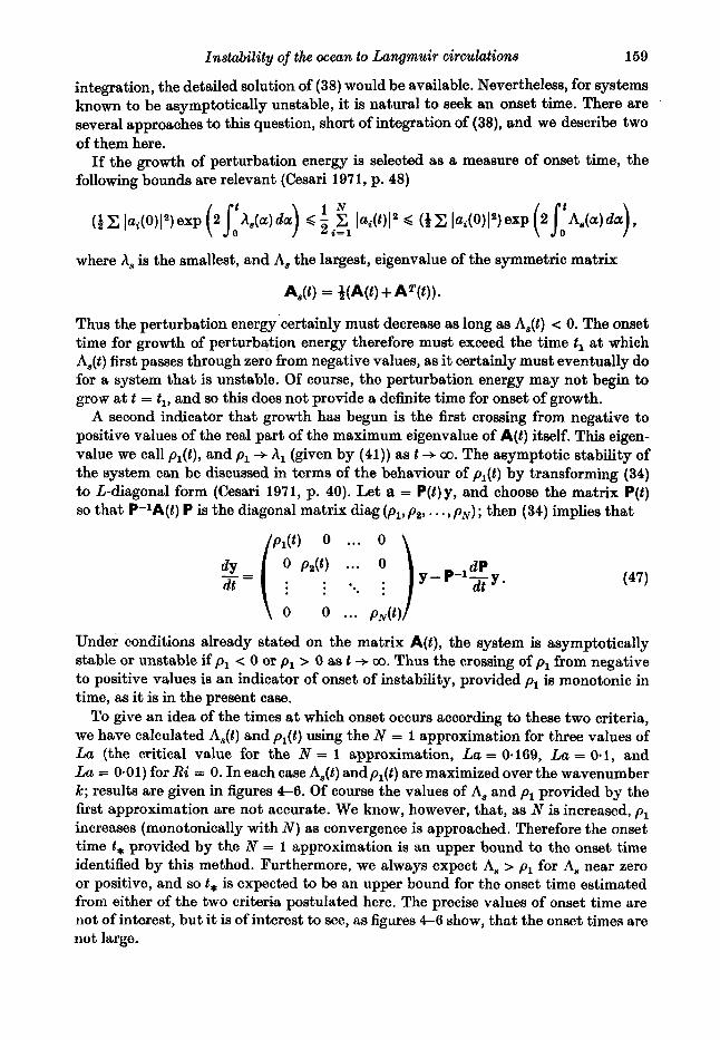
Instability of the ocean to Langmuir circulations 159
integration, the detailed solution of (38) would be available. Nevertheless, for systems known to be asymptotically unstable, it is natural to seek an onset time. There are several approaches to this question, short of integration of (38), and we describe two of them here.
If the growth of perturbation energy is selected as a measure of onset time, the following bounds are relevant (Cesari 197 1, p. 48)
where A, is the smallest, and A, the largest, eigenvalue of the symmetric matrix
AAt) = +(W +AT(t)).
Thus the perturbation energy'certainly must decrease as long as A,(t) < 0. The onset time for growth of perturbation energy therefore must exceed the time t , at which A,(t) first passes through zero from negative values, as it certainly must eventually do for a system that is unstable. Of course, the perturbation energy may not begin to grow a t t = t,, and so this does not provide a definite time for onset of growth.
A second indicator that growth has begun is the first crossing from negative to positive values of the real part of the maximum eigenvalue of A(t) itself. This eigen- value we call p l ( t ) , and p, + A, (given by (41)) as t -f a. The asymptotic stability of the system can be discussed in terms of the behaviour of pl ( t ) by transforming (34) to A-diagonal form (Cesari 1971, p. 40). Let a = P(t)y, and choose the matrix P ( t ) so that P-lA(t) P is the diagonal matrix diag (pl, p2, . . . , p N ) ; then (34) implies that
Under conditions already stated on the matrix A(t), the system is asymptotically stable or unstable if p1 -= 0 or p1 > 0 as t --f 00. Thus the crossing of p1 from negative to positive values is an indicator of onset of instability, provided p, is monotonic in time, as it is in the present case.
To give an idea of the times at which onset occurs according to these two criteria, we have calculated A,(t) and p l ( t ) using the N = 1 approximation for three values of La (the critical value for the N = 1 approximation, La = 0.169, La = 0.1, and La = 0.01) for Ri = 0. In each case A,(t) andp,(t) are maximized over the wavenumber k; results are given in figures 4-6. Of course the values of As and p1 provided by the first approximation are not accurate. We know, however, that, as N is increased, p, increases (monotonically with N) as convergence is approached. Therefore the onset time t , provided by the N = 1 approximation is an upper bound to the onset time identified by this met,hod. Furthermore, we always expect As > p, for A, near zero or positive, and so t , is expected to be an upper bound for the onset time estimated from either of the two criteria postulated here. The precise values of onset time are not of interest, but it is of interest to see, as figures 4-6 show, that t'he onset times are not large.

160 8. Leibovich and S. Paolucci
FIGURE 4. Eigenvalues A,(t) - - - - and p l ( t ) - are used to estimate the onset time for in- stability in Q ~ ( c ) , w calculated from the N = 1 Galerkin approximation, and for La = 0.169, which is the critical Langmuir number for the N = 1 approximation.
0.2
0.1
0
-0.1
-0.2
/ /
/ 1
/ I
I : I I
I I I
P I
FIGURE 5. Eigenvalues A&) ---- and p l ( t ) - for La = 0.1 and Ri = 0, calculated for N = 1. The time t* is designated in the text. m an upper bound for the onset time for instability.

Instability of the ocean to Langmuir circulations 161
0.1
0
FIGURE 6. Eigenvalues A,(t) - - - - and pl ( t ) - for La = 0.01 and Ri = 0, calculated for N = 1. The time t* is designated in the text as an upper bound for the onset time for instability for this (La, Ri) pair.
I I I I I I I I , 0.1 0.5 1 s 10 so 100 so0 1000
1, FIGURE 7. The upper bound, t * , for the onset time for instability aa a function of
La, for Ri = 0.
The upper bound for onset time based on p1 for Ri = 0 is displayed in a different way in figure 7 , which shows t , as a function of La.
( d ) Bounds on stable solutions As mentioned in subsection (b), i t is of interest to know that an asymptotically stable solution does not grow exceptionally large for finite values of time before eventually decaying. To establish the maximum size of the perturbations, we employ a slight variant of a standard analysis.

162 8. Leibovich and 8. Pmlucci
Let Q be the (constant) matrix with the eigenvectors of A as columns. Then (38) may be written as
where
Let
then
A, 0 ... !?- at - (0 :.- * . "i..c(t)x,
0 0 ... A,
C(t) = Q-lB(t) Q, a = Qx.
xi = xiexp[-A,t];
r, = A, - A, 3 0,
and (48) is equivalent to the integral equation
zi(t) = x&O) exp [ - r,t] + Cir(7) z,(T) exp [ - ri(t - T ) ] d ~ , l o t where Cir are the elements of C(t). Since r, 2 0,
Ilz(t)ll G IlX(0)ll +l1 IIC(7)II I I W I a7.
lIx(t)ll IlX(0)ll e-xp (/)C(T)Il d.).
0
By Gronwall's inequality and the definition of z
We have
and, since llcll II Q-YI II Qll II W)lI
for all 7 > 0, the asymptotic formula (43) is actually an upper bound for the matrix elements of B. If we let L be the N x N matrix with elements I,, given by (44), and let the positive constant c be
then (53)
(54)
If the flow is asymptotically stable, then Reh, = -p2 is negative. Perturbations may grow initially, but their norm is less than
IlX(0)ll exp [(c/2/3)21
a t any time, and certain decay occurs for t > p-2(c/2p)2. As the neutral curve is approached, p --f 0, and this estimate is not useful. We already know the solution is bounded but not asymptotically stable there, but we are unable by the present method to bound the solution for all values of t as /3 --+ 0.

Instability of the ocean to Langmuir circulations 163
5. Discussion Foster (1965, 1968) studied the linear instability of fluid subject to time-dependent
cooling at the upper surface for horizontal layers of both finite and infinite depths. Leibovich ( 1 9 7 7 ~ ) pointed out that the Langmuir circulation problem, even in water of constant density, is partially analogous to that of thermal convection; thus Foster’s problems and ours have interesting parallels that Craik (1977) has exploited.
Foster’s work deals with supercritical conditions only, and concentrates on the identification of an ‘onset ’ time for instability and the wavenumber of the most un- stable disturbance mode of the system as i t evolves in time in response to the imposed transient thermal boundary conditions. The method used involved a reduction (by a Galerkin approximation) to a set of ordinary differential equations in time, similar to that in our $4, followed by a numerical integration of these equations. The onset time is identified as that a t which the disturbance has amplified by an arbitrary factor (i,e., lorn, n = 1,2, etc.). Figures for the growth of a norm of the disturbance are given for cases (B) in which the temperature of the upper surface decreases monotonically with time. One other case (case (A), a step-function temperature decrease), was also treated, but presented in less detail. In case B disturbances increase supeiexponen- tially, and it therefore is the more dramatic; we note that the method of our f 4 cannot be applied to case B, since the limit of the associated matrix A(t) as t -+ co does not exist (hence the superexponential growth). The identification of the fastest growing, or most unstable, Fourier mode is of rather limited value, since the response curves (critical time for onset vs. horizontal wavenumber) are very flat. Nevertheless, Foster finds that the critical wavenumber changes little after disturbances are amplified by a factor of 10.
We have also attempted to identify a critical, or most unstable, mode for supercritical conditions, using the maximum eigenvalue pl(t; k , La, Ri) of $4. At any fixed Ri, La, and time level t exceeding the onset time t , of $4, p1 has a positive maximum when considered as a function of k. The locus of points in the k, La-1 plane at fixed t > t, and Ri describe the critical wavenumbers at fixed time. These curves rapidly approach that for t + 00, and are qualitatively like that curve; we therefore have displayed only the result for t = 00, which may be found in figures 1-3. Because of this rapid approach to the t = m curve, and because the most unstable wavenumbers for intermediate time do not deviate markedly from those for t = 00, the results illustrated can reasonably be described as the preferred modes of linear theory.
In the non-diffusive (La-’ --f co) stability analyses of steady currents Craik (1977) and Leibovich (1977b) found that all wavenumbers are unstable, and that the most unstable wavenumber is k = M). The present results are consistent with these con- clusions. It does not, however, appear as though the analogies with diffusive thermal instability tentatively offered in either paper, including Craik’s analogy with Foster’s (1965, 1968) time-dependent thermal-stability problem, agree very well with the present results. (For example, the most unstable wavenumbers differ considerably.) Since the mathematical problems differ from the present one, agreement is hardly to be expected, and we have not explored the matter further.
According to figure 1, the preferred mode of linear theory has dimensional wave- length A = (2n/0-32) k - l = 3-1Aw, where A, is the wavelength (2nlk) of the dominant surface waves, when La has t’he critical value 0.60 for linear instability. At the

104 8. Leibovich and S . Paolucci
Langmuir number, La = used in finite-difference calculations by LP, A 2: 0.25h,,.. Under such highly supercritical conditions, however, a correspondence between spacing of Langmuir circulation convergence zones and the wavelength of the preferred linear mode is not expected. In fact, the numerical simulations of LP suggest a cascade from smaller to larger cells, in agreement with the experimental findings of Faller & Caponi (1978), and this implies that one must know the lifetime of a circulation system, as well as wind conditions and sea state, to arrive at a (predicted) spacing of Langmuir convergence zones.
6. Conclusion The most important results of this paper are (a) the near coincidence of the asymp-
totic stability and global stability limits indicated in figures 1-3, and ( b ) the fact that these limits occur for La = O ( 1 ) for Richardson numbers of interest in the ocean (which are of order l O - l , according to the estimates of LP). Leibovich ( 1 9 7 7 4 argues that Langmuir numbers of interest in the ocean are small, typically of the order of 10-2-10-s. Consequently, the ocean is typically expected to be highly supercritical according to the present analysis.
It must be recognized, of course, that the present analysis deals with a highly idealized problem. It is assumed, for example, that motion begins from a quiescent state, so that the initial development is described by the solution (4) to the stress Rayleigh problem; in the ocean, current systems routinely occur that are not driven by the local wind field. In addition, the present analysis ignores the Coriolis accelera- tion which strongly affects the wind-driven current if the wind stress is maintained for sustained periods of time. (We are presently working on stability analyses and finite- difference simulations that include Coriolis effects.) Furthermore, the applied wind stress fluctuates in magnitude as well as direction, and is never constant as assumed here. A mean current system will develop that is associated, first of all, with the average applied wind stress. This current will presumably be subject to Langmuir circulation instabilities which form and decay as the local wind fluctuates in speed and direction. The mean current is then created not only by the average wind stress, but also by the Reynolds sbresses associated with the Langmuir instabilities (and, of course, to other phenomena, such as ordinary turbulence, that transfer momentum), which in turn depend upon the current and wind histories.
This work was supported by the Physical Oceanography Program of the National Science Foundation under Grant OCE 77-04482.
We are grateful to a referee for bringing the work of Homsy and his coworkers to our attention, and for other helpful remarks. Alex Craik read an early draft of the paper and suggested ways to clarify the presentation, and we appreciate his interest and constructive criticisms.
Appendix Convergence of the spectrum associated with the linear asymptotic stability prob-
lem as the number N of retained terms in the Galerkin expansion is increased is dealt with here. The eigenvalue with largest real part, A,, is of primary interest. Table 3

Instability of the ocean to Langmuir circulations 166
0 ; I I I I I I I I ...... ........ ...........
. . . . . . e . u - 8
. . . . . . " u - 5
. . . . . . ..-m-lO
. . . . . . . . e e x x n - l ]
. . . . . . . . * x ~ r - J 2
. . . . . . . . . .-xa-13
. . . . . . . . . .
N
1 6 6 7 8 9
10 11 12 13
5
6
N
- x a - 1 4
v
A1
- 0.27007 - 0.12267 - 0.1 1449 - 0.1 1176 - 0.10854 - 0.10743 - 0.10589 -0.10536 - 0.10453 - 0.10424
6.67 2-38 2.88 1.02 1.43 0.60 0.79 0.28
TABLE 3. Convergence of the maximum growth rate at k = 1.0, La = 0.4021, and Ri = 0 for the linear stability problem 88 t + 00.
shows the behaviour of A, for Ri = 0, k = 1.0 and La = 0.4021. The convergence is monotonic in all cases, as found also (table 1) for the relevant eigenvalue in the global stability analysis. The rate of convergence shown in table 3 is typical of that for other points in the (k, La, Ri) parameter space.
An N-term Galerkin approximation produces 3N eigenvalues. The real parts of the spectra for the example of table 3 (which is for a flow stable a t the prescribed wave- number) as N is increased is shown in figure 8. Real parts of complex conjugate pairs are indicated by crosse8; dots correspond to real eigenvalues. The spectrum grows more dense as N increaws, suggesting the filling in of a continuous spectrum. There is on indication, but no convincing evidence, that spectra lying wholly in the left- hand h plane (such as that in figure 8) are in general complex (except, because of

166 8. Leibovich and S. Paolucci
t-' FIGURE 9. Close-up view of the first eleven eigenvalues for the case in figure 8,
plotted in the complex plane.
symmetry about the real axis, for the eigenvalue with greatest real part). This com- plex, presumably continuous, spectrum takes form as N is increased in the following way. A pair of negative real eigenvalues move in from the left and presumably coalesce forming a double root that was never actually observed - and move off the real axis to form a complex conjugate pair. The farther from the imaginary axis the coalescence, occurs, the larger the ultimate value of the imaginary part. A close-up of the first eleven (of 39) eigenvalues for the N = 13 approximation of figure 8 is shown in figure 9.
The eigenvalue with largest real part is always real whether positive or negative; it appears in fact as though all eigenvalues that cross the imaginary axis do so through the real line. Unstable configurations therefore appear associated with a real, discrete spectrum in the right half-plane as well as a continuous spectrum in the left half-plane. It is not clear, however, whether the eigenvalues that cross the imaginary axis peel off the continuous spectrum in the left-hand plane very close to the origin, or a t the origin itself.
All numerical calculations were performed in double precision on an IBM 370/ 168 using the Fortran H compiler with optimization parameter set a t 2. We believe the eigenvalues calculated as part of the construction of stability diagrams are subject to less than a 1% error.
R E F E R E N C E S
BELLMAN, R. 1969 Stability Theory of Diflerential Equations. Dover. CESARI, L. 1971 Aqmptotic Behavior and Stability Problems in Ordinary Differentid Equation%,
3rd ed. Springer. CRAIK, A. D. D. 1977 The generation of Langmuir circulations by an instability mechanism.
J. Fluid Mech. 81, 209-223. CRAIK, A. D. D. & LEIBOVICH, S. 1976 A rational model for Langmuir circulations. J. Fluid
Mech. 73, 401-426. DUDIS, J. J. & DAVIS, S. H. 1971a Energy stability of the buoyancy boundary layer. J.Pluid
Mech. 47, 381-403. DUDIS, J. J. & DAVIS, S. H. 1971b Energy stability of the Ekman boundary layer. J. Fluid
Mech. 47, 405-413. FALLER, A. J. 1978 Experiments with controlled Langmuir circulations. Science 201, 618-620. FALLER, A. J. & CAPONI, E. A. 1978 Laboratory studies of wind driven Langmuir circulations.
J . Qeophys. Res. 83, 3617-3633.

Instability of the ocean to Langmuir circulatims 167
FINLAYSON, B. A. 1972 The Method of Weighted Residuals and Varhtional Principles. Academic. FOSTER, T. D. 1965 Stability of a homogeneous fluid cooled uniformly from above. Phys. Fluids
FOSTER, T. D. 1968 Effect of boundary conditions on the onset of convection. Phys. Fluids 11,
GALDI, G. P. & RIONERO, S. 1977 On magnetohydrodynamic motions in unbounded domains:
GUYERYAN, R. J. & HOMSY, G. M. 1975 The stability of uniformly accelerated flows with appli-
HOYSY, G. M. 1973 Global stability of time-dependent flows: impulsively heated or cooled liquid
JOSEPH, D. D. 1976a Stability of Fluid Motiona I. Springer. JOSEPE, D. D. 1970b Stability of Fluid Motwna I I . Springer. LANGMUIR, I. 1938 Surface motion of water induced by wind. Science 87, 119-123. LEIBOVICH, S. 1977a On the evolution of the system of wind drift currents and Langmuir
circulations in the ocean. Part 1. Theory and averaged current. J. Fluad Mech. 79, 715-743. LEIBOVICH, 5. 1977 b Convective instability of stably stratified water in the ocean. J. Fluid Mech.
LEIBOVICH, 5. 1980 On wave-current interaction theories of Langmuir circulations. J. .Fluid Mech. 99, 715-724.
LEIBOVICH, S. & PAOLUCCI, S. 1980 The Langmuir circulation instability as amixing mechanim in the upper ocean. J. Phys. Ocean. 10, 186-207.
LEIBOVICH, S. & RADMKRISHNAN, K. 1977 On the evolution of the system of wind drift cur- rents and Lmgmuir Circulations in the ocean. Part 2. Structure of the Langmuir vortices. J. Fluid Mech. 80, 481-507.
WANKAT, P. C. & HOMSY, G. M. 1977 Lower bounds for the onset time of instability in heated layers. Phys. Pliiids 20, 1200-1201.
8, 1249-1257.
1257- 1262.
stability and uniqueness. Ann. Mat. Pura & AppE. 115, 119-154.
cation to convection driven by surface tension. J. Fluid Mwh. 68, 191-207.
layers. J. Fluid Mech. 60, 129-139.
82,561-585.