1

The influence of the global photochemical composition of the

troposphere on European summer smog, Part I: Application of a

global to mesoscale model chain

Bärbel Langmann1), Susanne E. Bauer2), and Isabelle Bey3)

1) Max-Planck-Institut für Meteorologie, Bundesstr. 55, D-20146 Hamburg, Germany, e-mail: langmann@dkrz.de

2) Laboratoire des Sciences du Climat et de l’Environnement (LSCE), CEA-CNRS,CE

SACLAY, L'Orme des Merisiers, F-91191 Gif-sur Yvette Cedex, France, e-mail: bauer@lsce.saclay.cea.fr

3) Swiss Federal Institute of Technology (EPFL), EPFL-ENAC-LMCA, Batiment Chimie,

CH-1015 Lausanne, Switzerland, e-mail: isabelle.bey@epfl.ch

published in Journal of Geophysical Research, Atmospheres,

Vol. 108, D4, 4146, doi:10.1029/2002jd002072,2003

2

Abstract Elevated mixing ratios of ozone in the lower troposphere are a major summer time air

pollution issue in Europe. Photochemical in-situ production of ozone is the most important

source in the planetary boundary layer and has been studied extensively. However, the

contributions of background ozone due to stratospheric intrusions, lightning nitrogen oxide

followed by ozone production, convective mixing and intercontinental transport are still

poorly quantified. We analyse in this paper the influence of the large-scale ozone background

on near-surface ozone throughout a summer smog period in July 1994 over Europe. For this

purpose a chain of global to mesoscale models is applied with a nesting procedure coupling

the individual model simulations. It is found that background ozone as determined by the

global model dominates the results of the higher resolution limited area models increasingly

with height. Strong convective events like thunderstorms couple free tropospheric and

planetary boundary layer air masses so that ozone from above is injected into the planetary

boundary layer contributing an amount of 5-10 ppbv to near-surface ozone in the afternoon

hours. A decrease in the same range of 5-10 ppbv in maximum near-surface ozone over

Central Europe is found in a model simulation where European anthropogenic emissions are

reduced by 25 %, an amount equal to the reported emission trends in Germany from 1994 to

2000. We conclude that intercontinental transport of pollution can obscure the results of local

efforts to reduce critical exposure levels of ozone.

3

1. Introduction

Enhanced concentrations of photooxidants appear episodically in the planetary boundary layer

(PBL) in summertime during high pressure episodes when direct solar irradiation raises near-

surface temperatures. In industrialised regions emissions of photooxidant precursor

substances from fossil fuel combustion (NOx: the sum of NO and NO2, and VOC’s: volatile

organic carbons) and their photochemical transformations are mainly responsible for elevated

and episodically critical levels of near-surface ozone and other photooxidants with

consequences for human health and plant damages.

When thinking about protection policies, e. g. governmental restrictions or guidelines for

reduction of industry and traffic emissions during such episodes or on even longer time scales,

numerical model simulations help to estimate the potential effects of emission reduction

strategies. A huge number of limited area models covering the regions of interest, e. g. Europe

or North America, have been applied to guide decision makers (Russell and Dennis, 2000).

The quality of these models is usually tested in hindcast experiments where the calculated

distributions of atmospheric trace species are evaluated with available measurements. For

such model simulations detailed inventories of emission fluxes are necessary and the

meteorological situation of a specific period of interest should be reproduced as realistically

as possible. In addition to anthropogenic emissions, biogenic emission fluxes of hydrocarbons

have to be specified – although highly uncertain today (Simpson et al., 1999) – because these

photooxidant precursors often dominate over anthropogenically emitted hydrocarbons,

especially during summer smog episodes (Chameides et al., 1988).

Another poorly known topic is the long-range transport of polluted air masses. Stratosphere-

troposphere exchange due to irreversible mixing within tropopause folds and / or cut-off lows

4

contribute to the long-range transport and elevated ozone levels in the troposphere (Stohl and

Trickl, 1999), sometimes far away from the region of origin. But the overall contribution of

stratospheric ozone to the tropospheric ozone budget is still uncertain (Roelofs and Lelieveld,

1997). The importance of intercontinental transport of photooxidants and precursors in mid-

latitudes - from Asia to North America (Jaffe et al., 1999, Jacob et al., 1999) and North

America to Europe (Li et al., 2001) has been recently emphasised again after first speculations

by Parrish et al. (1993). In this context anthropogenic emissions from industry and traffic and

biogenic VOC emissions released into the PBL of North America have to be considered –

when we focus on Europe, as well as aircraft emissions, NO production by lightning and

emissions from forest fires. An impact of Canadian forest fire emissions on Europe

throughout the whole summer season is believed to be probable (Forster et al., 2001).

Although it is evident that single continents are not photochemically isolated from the global

troposphere, numerical studies with limited area models for Europe or North America have

neglected the influence of intercontinental transport of polluted air masses until now. The

reason is a lack of detailed information about trace species concentrations throughout the

troposphere. Unfortunately, a global observation network including surface based and satellite

measurements as it exists for meteorological variables is not yet available for tropospheric

trace species. However, within the next few years substantial progress in satellite observations

of the tropospheric chemical composition can be expected including vertically resolved

information (Singh and Jacob, 2000). An option that is available today to investigate the large

scale distribution of trace species and their temporal and spatial variability in limited area

models is a global-regional nesting approach as it is also applied for weather forecast

simulations: large scale phenomena are simulated by global coarse grid models and the results

are used to provide background concentrations for higher resolution limited area model

simulations over the regions of interest.

5

In this paper, a summer smog episode occurring over Europe at the end of July 1994 is

analysed with a global to mesoscale model chain. To our knowledge it is the first time that

such a model chain from the global to the mesoscale is used to investigate the question how

long-range transport can affect ozone mixing ratios in surface air over Europe during summer

smog episodes. Previous studies of this specific episode have been carried out with prescribed

climatological trace species mixing ratios at the lateral model boundaries of a European wide

simulation (Bauer and Langmann, 2002b). These simulations excellently reproduced

measured near-surface ozone and nitrogen dioxide mixing ratios at urban stations, whereas in

rural areas ozone within the PBL was underestimated. A dramatic underprediction of ozone

mixing ratios was also found in the free troposphere. It was suggested that the free

troposphere over Europe was significantly influenced by long-range transport of ozone from

outside of Europe. Intense convective activity and vertical mixing during this smog episode

coupled the PBL and the free troposphere so that the impact of background ozone on near-

surface ozone was far from being negligible (Langmann and Bauer, 2002). In order to arrive

at more realistic estimates of the photochemical composition of the troposphere over Europe,

we repeated these calculations with time resolved data from a global chemistry transport

model (Bey et al., 2001). The models and their set-ups are introduced in section 2. In section 3

model results are analysed. The individual model strengths and weaknesses are assessed and

the powerful application of the combined global to mesoscale model chain is presented. An

additional sensitivity simulation is shown which compares the contribution of long-range

transported pollution to ozone concentrations at the surface with the effect on ozone levels

obtained from local emission reductions. Finally, section 4 draws conclusions and gives an

outlook. A detailed analysis of the processes responsible for elevated ozone mixing ratios

over Europe in July 1994 is given in a second paper (Langmann and Bey, 2002).

6

2. Model descriptions and set-ups

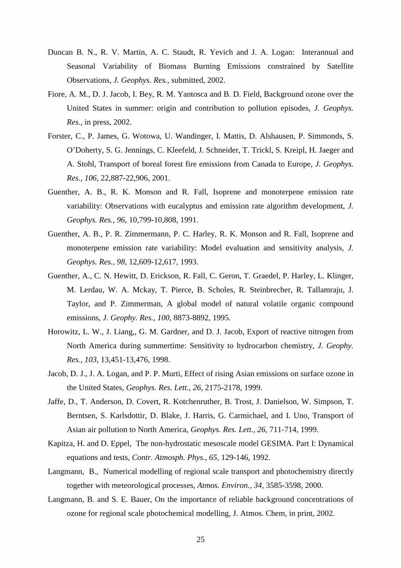
The global to mesoscale model chain used in this study consists of three Eulerian models with

a total of four resolutions (Fig. 1): The global chemistry-transport model GEOS-CHEM (Bey

et al., 2001), the regional atmosphere-chemistry model REMO (Langmann, 2000) applied in

two resolutions and the non-hydrostatic mesoscale atmosphere-chemistry model GESIMA

(Bauer and Langmann, 2002a). The simulations with the individual models are carried out one

after the other. They are connected by a one-way nesting procedure. Although a nesting factor

(ratio of coarse model resolution to nested model resolution) of 3 is referred to as optimal

value by Pleim et al. (1991) we use nesting factors of 9, 3 and 4.5, respectively. For the

global-European nesting step we had no better choice because no other global model

simulation was available. For comparison with the global to mesoscale model chain, a

mesoscale mode chain is run separately (see Fig. 1) using fixed climatological trace species

distributions for the initialisation and at the lateral boundaries of the European wide

simulation. The individual models and set-ups are described only briefly. More detailed

information and evaluations can be obtained from the above cited references.

Figure 1

2.1. The global model GEOS-CHEM

The global chemistry-transport model GEOS-CHEM (Bey et al., 2001) is driven by

assimilated meteorological observations provided by the Goddard Earth Observing System

(GEOS) of the NASA Data Assimilation Office. The data are available every 6 hours on

sigma coordinates with 20 vertical levels up to 10 hPa. The horizontal resolution is 2ο in

latitude and 2.5ο in longitude. For computational expediency the GEOS-CHEM simulation is

7

carried out over a 4ο x 5ο grid with horizontally averaged GEOS data. Advection of 24

chemical trace species is computed every 30 minutes with a flux-form semi-Lagrangian

method as described by Lin and Rood (1996). Moist convection is determined after Allen et

al. (1996a, b) using the GEOS convective, entrainment and detrainment mass fluxes. Within

the atmospheric mixed layer full mixing is assumed diagnosed from surface instability. The

tropospheric chemical mechanism of GEOS-CHEM is an updated version of Horowitz et al.

(1998). It includes 80 species and 150 reactions with detailed photooxidation schemes for the

major hydrocarbons including isoprene. Dry deposition of oxidants and water soluble species

is computed using a modified version of Wesley (1989). Anthropogenic emissions are

distributed on the basis of inventories for 1985 as described in Wang et al. (1998) with

updates for 1994 based on energy use statistics as described in Bey et al. (2001). Biomass

burning emissions are derived from a climatological inventory (Wang et al., 1998), biogenic

emissions are determined with a modified version of the GEIA inventory (Guenther et al.,

1995) and NO production by lightning is calculated as described in Wang et al. (1998). A

general evaluation of the GEOS-CHEM model has been previously carried out using

observations from surface sites, NASA/GTE aircraft campaigns, and ozonesondes [Bey et al.,

2001]. No global bias was found for the key species (e.g. ozone, NO, or PAN) except for CO

concentrations which were systematically underestimated by 10 to 20 ppb.

The GEOS-CHEM simulation is conducted from June, 1, 1993 to August, 31, 1994 starting

from climatological trace species distributions as initial conditions. This provides a one-year

initialisation until June 1994. Model results from July 1994 are used in this study for

comparison with observations and for the nesting of the higher resolution European wide

REMO simulation.

8

2.2. The regional model REMO

The regional on-line atmosphere-chemistry model REMO (Langmann, 2000) determines at

every model time step the physical and chemical state of the model atmosphere. The

dynamical part and the physical parameterisation routines are taken from the regional weather

forecast model system EM/DM of the German Weather Service (Majewski, 1991). In the

current study the REMO model is applied with 20 vertical layers of increasing thickness

between the Earth surface and the 10 hPa pressure level using terrain following hybrid

pressure-sigma coordinates. The horizontal resolution is 0.5ο for the model domain covering

Europe and 1/6ο for the smaller area covering Germany (Fig. 1). The corresponding model

time steps are 5 and 2 minutes, respectively. The prognostic equations for surface pressure,

temperature, specific humidity, cloud water, horizontal wind components and chemical trace

species mixing ratios are written on an Arakawa-C-grid (Mesinger and Arakawa, 1976).

Tracer transport of 39 species is represented by horizontal and vertical advection according to

the algorithm of Smolarkiewitz (1983), convective up- and downdraft by a modified scheme

of Tiedtke (1989), vertical diffusion after Mellor and Yamada (1974) and dry deposition after

Wesley (1989). The RADM II chemical scheme (Stockwell et al. 1990) describes

photochemical production and loss of 63 compounds by 163 chemical reactions in the gas

phase including a wide range of hydrocarbon degradation reactions. Aqueous phase chemistry

processes and wet removal are implemented according to Walcek and Taylor (1986).

Photolysis rates are calculated as described in Madronich (1987) and Chang et al. (1987).

Anthropogenic emission data are provided by the Institute of Energy Economics and the

Rational Use of Energy, Stuttgart, Germany (B. Wickert, personal communication) in 1/2ο

resolution for the European model area and consistently in 1/6ο resolution for the German

model area. Biogenic VOC emissions are determined based on Guenther et al. (1991, 1993).

9

To force the two REMO model simulations focussing on Europe and Germany to stay close to

the real weather situation, time varying fields of surface pressure, temperature, horizontal

wind velocities and moisture derived from the meteorological analysis data of the German

Weather Service are used as initial and boundary information, updated every 6 hours. The

model is run in the forecast mode with respect to the model physics. Starting at 0 UTC every

day a 30 hour forecast is computed. The first six hours of the consecutive meteorological only

forecasts are neglected to account for a spin-up time. During the following 24 hours

atmospheric physics and chemistry are calculated continuously. At 6 UTC on the following

day a discontinuity in the physical state of the model atmosphere is introduced due to the new

daily meteorological forecast, whereas tropospheric chemistry is calculated continuously

during the period from July 20, 12 UTC to July 30, 12 UTC, 1994.

Table 1

The temporal and spatial variability of trace species mixing ratios for the initialisation and at

the lateral boundaries of the European wide REMO simulation is provided by the output of

the global GEOS-CHEM simulation. The chemical mechanisms of the GEOS-CHEM and the

REMO model are different, especially with respect to the organic part. Alkane chemistry is of

comparable complexity in both models. Alkene chemistry is represented by 4 classes in the

REMO model and by only 2 classes in the GEOS-CHEM model, however the latter has more

detailed representation of isoprene chemistry. Three aromatic species (touluene, xylene and

cresol) are included in the REMO model, whereas the GEOS-CHEM model neglects aromatic

chemistry because of the short species lifetimes. Although we are aware this introduces

inconsistencies, we use all available trace species mixing ratio information from the global

GEOS-CHEM simulation to initialise the European wide simulation with REMO. These

mixing ratios are distributed among the 39 prognostic species of the regional model as

10

summarised in Tab. 1. The major longer-lived photooxidant and precursor mixing ratios as for

O3, CO, H2O2, PAN, C2H6 are provided by GEOS-CHEM. The GEOS-CHEM concentrations

are interpolated horizontally and vertically to the REMO 1/2ο grid following the temperature

interpolation technique of Majewski (1985). For those compounds missing in GEOS-CHEM

but necessary for the REMO initialisation and at its lateral boundaries, vertical profiles are

derived from available measurements during recent years. The mixing ratios of the short-lived

compounds are set to zero. GEOS-CHEM provides tracer information in 12 hour intervals at 0

and 12 UTC. A linear interpolation in time is carried out to determine the lateral boundary

information for the European wide simulation throughout the episode. The 39 chemical trace

species mixing ratios are transported by advection across the limited area models lateral

boundaries as described in Pleim et al. (1991). Results from this simulation are hereafter

denoted as REMO 1/2ο.

An additional European wide REMO simulation is carried out with climatological trace

species assumptions for the initialisation and at the lateral model boundaries which

corresponds to the usual set-up for limited area model simulations. Model results from this

latter configuration are denoted with an asterisk in the following sections: *REMO 1/2ο. For

the next nesting step which is the German wide REMO 1/6ο simulation nested into the

European wide REMO 1/2ο simulation the information of the 39 chemical variables is

available with a time resolution of one hour. Once again two REMO simulations are carried

out: one as part of the global to mesoscale model chain (REMO 1/6ο), the other one as part of

the mesoscale model chain (*REMO 1/6ο).

2.3. The mesoscale model GESIMA

11

The 4 km x 4 km non-hydrostatic meso-γ-scale on-line atmosphere-chemistry model

GESIMA (Bauer and Langmann, 2002a) is applied over the area of Berlin-Brandenburg,

Germany. A detailed description of the dynamical part is given in Kapitza and Eppel (1992).

For the numerical solution, the thermodynamic variables are split into isentropic reference

values which are assumed to be hydrostatic, and deviations. For the density, the Boussinesq

approximation is used. The model equations are discretised on terrain following coordinates

with 25 levels in the vertical up to 11 km height. The basic model time step is 20 seconds. For

the horizontal representation orthogonal coordinates with an Arakawa-C-grid are used.

Advection of trace species is determined according to Smolarkiewitz (1984), vertical

diffusion is calculated using a first order closure scheme according to level 2.5 (Mellor and

Yamada, 1974) and dry deposition is computed after Wesley (1989). Gasphase chemical

mechanism, photolysis rates, anthropogenic and biogenic emissions are included in the

GESIMA model in the same way as already introduced above for the REMO model.

The GESIMA model uses the following interpolated results of the German wide REMO 1/6ο

simulation for initialisation: horizontal wind velocities, potential temperature, specific

humidity, pressure and trace species mixing ratios. Throughout the simulation (July, 22 – 26,

1994) the information of the meteorological variables is nudged at the lateral and top

boundaries of the GESIMA model, whereas the information of the chemical species is nested

according to Pleim et al. (1991). The data sets are updated every hour with a linear

interpolation in between. For more details see Bauer (2000).

3. Model results and discussion

In this section model results and comparisons with observations are presented and discussed

for the period of July, 20-30, 1994. We focus on ozone for three reasons: 1) ozone is

12

associated with summer smog, 2) plentiful ozone measurements are available, and 3) ozone is

subject of long-range transport in the free troposphere.

3.1. Weather situation over Europe

The July 1994 episode was characterised by high surface pressure over Central Europe

causing heat waves with maximum near-surface temperatures nearly reaching the highest

temperatures ever measured since the beginning of the daily temperature records (Berliner

Wetterkarte, 1994). Several low pressure systems passed over the British Isles and

Scandinavia. In the PBL over Central Europe low easterly winds prevailed whereas the free

tropospheric air masses over Central Europe originated from western directions from the

Atlantic ocean. Until 25 July dry continental air masses without clouds dominated the weather

situation over Central Europe. On 25 July an occlusion with strongly decreasing intensity

entered Germany from the west, accompanied by moist subtropical air and thunderstorms.

During the following days the weather situation remained moist and hot until 29 July, when

fresh maritime air was transported towards Germany. Overall, the weather situation favoured

photosmog formation and accumulation in the PBL over Central Europe.

3.2. Large scale distribution of ozone outside of Europe

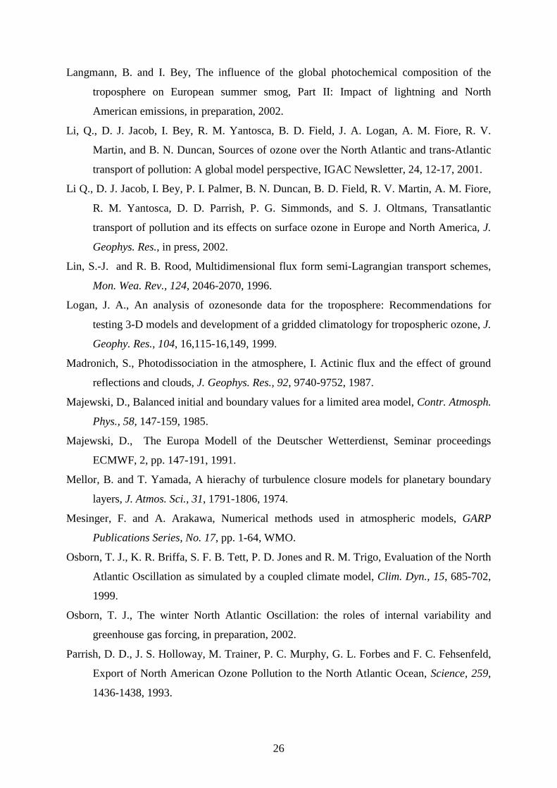
The spatial and temporal variability of ozone mixing ratios as determined by the GEOS-

CHEM model at three locations in the Atlantic ocean at [20N, 20W], [50N, 20W] and [80N,

20W] is shown in Fig. 2 to demonstrate the conditions of the air masses advected towards

Europe. The increase of ozone mixing ratios above the tropopause clearly indicate the decline

of the tropopause altitude with increasing latitude from about 13 km to less than 8 km.

Throughout the troposphere a pronounced day-to-day variability of ozone mixing ratios of up

to 20 ppbv is visible along the longitude of 20W. PBL mixing ratios at [20N, 20W] and [80N,

20W] were influenced by the nearby landmasses whereas at [50N, 20W] maritime conditions

13

prevail in the PBL. The influence of the temporal and spatial fluctuations of ozone mixing

ratios in the downwind direction of Europe on the European photochemical composition in

the troposphere is further elucidated in the following section.

Figure 2

3.3. Ozone over Europe

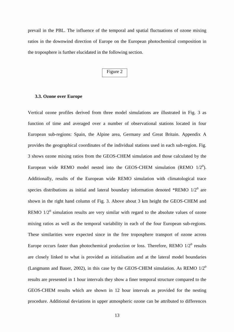
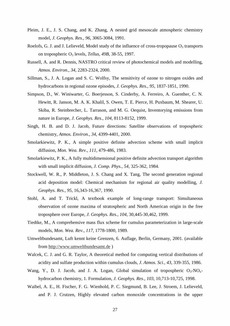
Vertical ozone profiles derived from three model simulations are illustrated in Fig. 3 as

function of time and averaged over a number of observational stations located in four

European sub-regions: Spain, the Alpine area, Germany and Great Britain. Appendix A

provides the geographical coordinates of the individual stations used in each sub-region. Fig.

3 shows ozone mixing ratios from the GEOS-CHEM simulation and those calculated by the

European wide REMO model nested into the GEOS-CHEM simulation (REMO 1/2ο).

Additionally, results of the European wide REMO simulation with climatological trace

species distributions as initial and lateral boundary information denoted *REMO 1/2ο are

shown in the right hand column of Fig. 3. Above about 3 km height the GEOS-CHEM and

REMO 1/2ο simulation results are very similar with regard to the absolute values of ozone

mixing ratios as well as the temporal variability in each of the four European sub-regions.

These similarities were expected since in the free troposphere transport of ozone across

Europe occurs faster than photochemical production or loss. Therefore, REMO 1/2ο results

are closely linked to what is provided as initialisation and at the lateral model boundaries

(Langmann and Bauer, 2002), in this case by the GEOS-CHEM simulation. As REMO 1/2ο

results are presented in 1 hour intervals they show a finer temporal structure compared to the

GEOS-CHEM results which are shown in 12 hour intervals as provided for the nesting

procedure. Additional deviations in upper atmospheric ozone can be attributed to differences

14

in the strength and location of convective mixing by the numerous thunderstorms in the two

simulations. These differences in the meteorology of the GEOS-CHEM and REMO 1/2ο

simulations are caused by a factor of nine difference in the horizontal resolutions, the different

analysis data sets used to drive the two models and the different model philosophies (CTM /

on-line Atmosphere-Chemistry Model).

Figure 3

*REMO 1/2ο simulation results for ozone mixing ratios (Fig. 3, right hand column) above 3

km height are completely different from and considerably smaller than the above discussed

ozone mixing ratios as determined by GEOS-CHEM and REMO 1/2ο. In this case the fixed

climatological trace species profiles chosen for the initialisation and at the lateral model

boundaries mainly determine *REMO 1/2ο results in that altitude region. Hence, the

importance of reliable assumptions for background mixing ratios is emphasised.

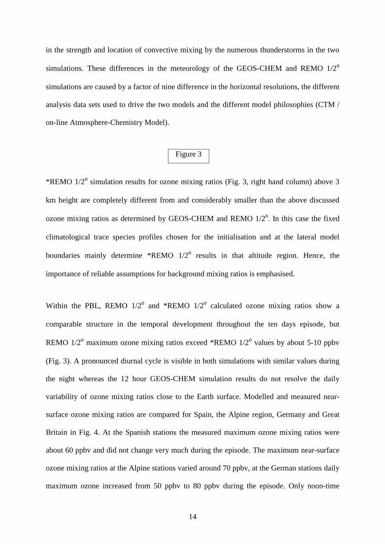
Within the PBL, REMO 1/2ο and *REMO 1/2ο calculated ozone mixing ratios show a

comparable structure in the temporal development throughout the ten days episode, but

REMO 1/2ο maximum ozone mixing ratios exceed *REMO 1/2ο values by about 5-10 ppbv

(Fig. 3). A pronounced diurnal cycle is visible in both simulations with similar values during

the night whereas the 12 hour GEOS-CHEM simulation results do not resolve the daily

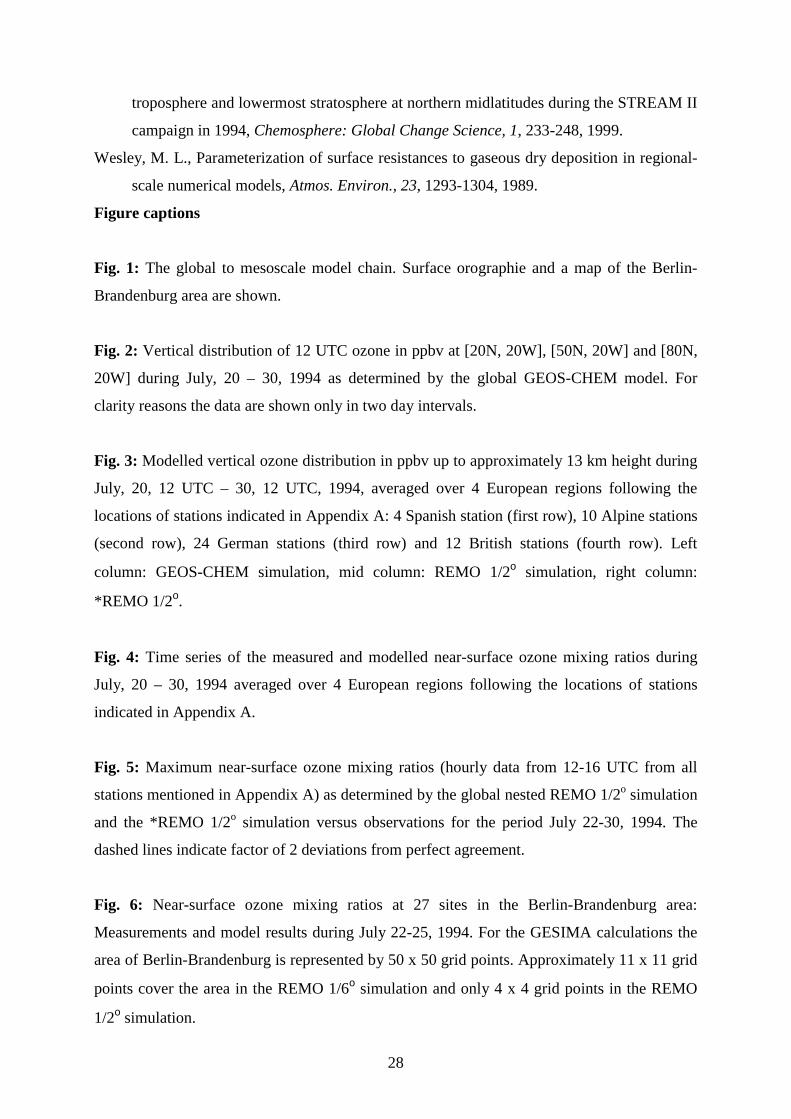
variability of ozone mixing ratios close to the Earth surface. Modelled and measured near-

surface ozone mixing ratios are compared for Spain, the Alpine region, Germany and Great

Britain in Fig. 4. At the Spanish stations the measured maximum ozone mixing ratios were

about 60 ppbv and did not change very much during the episode. The maximum near-surface

ozone mixing ratios at the Alpine stations varied around 70 ppbv, at the German stations daily

maximum ozone increased from 50 ppbv to 80 ppbv during the episode. Only noon-time

15

values are shown for the GEOS-CHEM simulation because the model does not resolve well

the diurnal cycle at continental sites. GEOS-CHEM calculated values reproduce fairly well

the measurements at 12 UTC including the difference of 10 ppbv in maximum ozone between

the Spanish and Alpine regions and the ozone increase at the German stations taking into

account that maximum near-surface ozone mixing ratios are reached later in the afternoon. At

the British stations daily maximum ozone values are generally overpredicted by up to 25

ppbv by the GEOS-CHEM model. Despite this high bias, the coarse resolution of GEOS-

CHEM simulation is able to capture the day-to-day fluctuations in ozone mixing ratios until

the 25th, the less polluted situation afterwards and the rebuild of maximum ozone on the 29th.

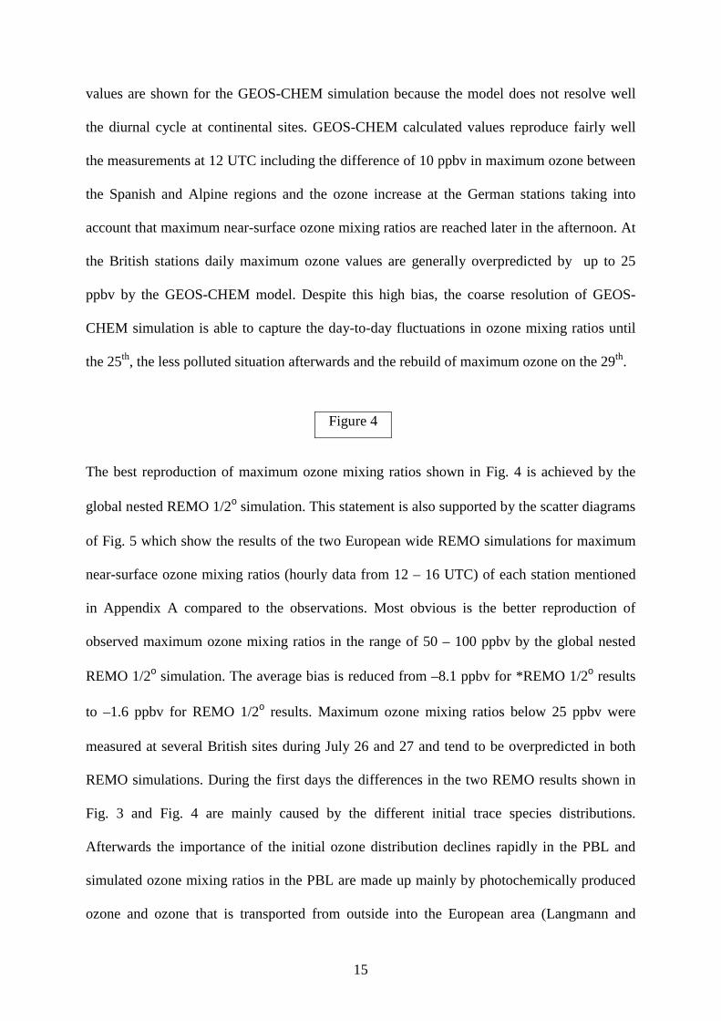
The best reproduction of maximum ozone mixing ratios shown in Fig. 4 is achieved by the

global nested REMO 1/2ο simulation. This statement is also supported by the scatter diagrams

of Fig. 5 which show the results of the two European wide REMO simulations for maximum

near-surface ozone mixing ratios (hourly data from 12 – 16 UTC) of each station mentioned

in Appendix A compared to the observations. Most obvious is the better reproduction of

observed maximum ozone mixing ratios in the range of 50 – 100 ppbv by the global nested

REMO 1/2ο simulation. The average bias is reduced from –8.1 ppbv for *REMO 1/2ο results

to –1.6 ppbv for REMO 1/2ο results. Maximum ozone mixing ratios below 25 ppbv were

measured at several British sites during July 26 and 27 and tend to be overpredicted in both

REMO simulations. During the first days the differences in the two REMO results shown in

Fig. 3 and Fig. 4 are mainly caused by the different initial trace species distributions.

Afterwards the importance of the initial ozone distribution declines rapidly in the PBL and

simulated ozone mixing ratios in the PBL are made up mainly by photochemically produced

ozone and ozone that is transported from outside into the European area (Langmann and

Figure 4

16

Bauer, 2002). As the background mixing ratios are the only difference between the two

REMO simulations, they are also responsible for the differences in the calculated near-surface

ozone mixing ratios. Therefore it can be concluded that during the summer smog episode

investigated here, vertical exchange between PBL and free troposphere air masses clearly

took place. A significant portion (5-10 %) of near-surface maximum ozone during that

episode did not build up from local anthropogenic or biogenic emissions but were due to

transport of background ozone from the free troposphere. Our study emphasises the need for

using realistic background ozone concentrations throughout the troposphere – which might be

different from the climatological values in some cases such as the episode described here – to

reduce uncertainties in the simulation of ozone concentrations in the PBL.

Figure 5

The importance of convective events and accompanying rapid subsidence in bringing

background ozone from the free troposphere into the PBL is also emphasised by Fiore et al.

(2002) who studied the origin and contribution of background ozone to photochemical

pollution events in the United States during summer. The authors report a contribution of

intercontinental transport from Asian and European anthropogenic sources on surface ozone

in the United States of 4-7 ppbv in average.

3.4. Photooxidants in the Berlin-Brandenburg area

For further comparisons of model results and measurements we focus on the area of Berlin-

Brandenburg (Fig. 1) where a field experiment called FLUMOB (German abbreviation of

Aircraft measurements of ozone and precursors to estimate emission reduction measures in

Berlin-Brandenburg) took place at the end of July 1994 (Stark et al., 1995). Aircraft

measurements, near-surface measurements and a few vertical soundings were carried out from

17

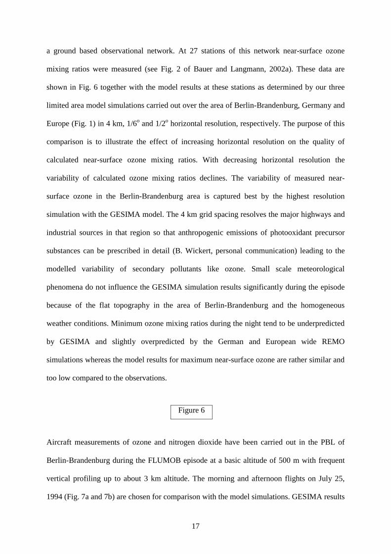
a ground based observational network. At 27 stations of this network near-surface ozone

mixing ratios were measured (see Fig. 2 of Bauer and Langmann, 2002a). These data are

shown in Fig. 6 together with the model results at these stations as determined by our three

limited area model simulations carried out over the area of Berlin-Brandenburg, Germany and

Europe (Fig. 1) in 4 km, 1/6o and 1/2o horizontal resolution, respectively. The purpose of this

comparison is to illustrate the effect of increasing horizontal resolution on the quality of

calculated near-surface ozone mixing ratios. With decreasing horizontal resolution the

variability of calculated ozone mixing ratios declines. The variability of measured near-

surface ozone in the Berlin-Brandenburg area is captured best by the highest resolution

simulation with the GESIMA model. The 4 km grid spacing resolves the major highways and

industrial sources in that region so that anthropogenic emissions of photooxidant precursor

substances can be prescribed in detail (B. Wickert, personal communication) leading to the

modelled variability of secondary pollutants like ozone. Small scale meteorological

phenomena do not influence the GESIMA simulation results significantly during the episode

because of the flat topography in the area of Berlin-Brandenburg and the homogeneous

weather conditions. Minimum ozone mixing ratios during the night tend to be underpredicted

by GESIMA and slightly overpredicted by the German and European wide REMO

simulations whereas the model results for maximum near-surface ozone are rather similar and

too low compared to the observations.

Figure 6

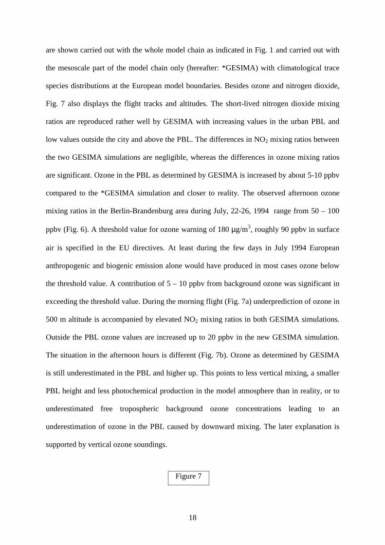
Aircraft measurements of ozone and nitrogen dioxide have been carried out in the PBL of

Berlin-Brandenburg during the FLUMOB episode at a basic altitude of 500 m with frequent

vertical profiling up to about 3 km altitude. The morning and afternoon flights on July 25,

1994 (Fig. 7a and 7b) are chosen for comparison with the model simulations. GESIMA results

18

are shown carried out with the whole model chain as indicated in Fig. 1 and carried out with

the mesoscale part of the model chain only (hereafter: *GESIMA) with climatological trace

species distributions at the European model boundaries. Besides ozone and nitrogen dioxide,

Fig. 7 also displays the flight tracks and altitudes. The short-lived nitrogen dioxide mixing

ratios are reproduced rather well by GESIMA with increasing values in the urban PBL and

low values outside the city and above the PBL. The differences in NO2 mixing ratios between

the two GESIMA simulations are negligible, whereas the differences in ozone mixing ratios

are significant. Ozone in the PBL as determined by GESIMA is increased by about 5-10 ppbv

compared to the *GESIMA simulation and closer to reality. The observed afternoon ozone

mixing ratios in the Berlin-Brandenburg area during July, 22-26, 1994 range from 50 – 100

ppbv (Fig. 6). A threshold value for ozone warning of 180 µg/m3, roughly 90 ppbv in surface

air is specified in the EU directives. At least during the few days in July 1994 European

anthropogenic and biogenic emission alone would have produced in most cases ozone below

the threshold value. A contribution of 5 – 10 ppbv from background ozone was significant in

exceeding the threshold value. During the morning flight (Fig. 7a) underprediction of ozone in

500 m altitude is accompanied by elevated NO2 mixing ratios in both GESIMA simulations.

Outside the PBL ozone values are increased up to 20 ppbv in the new GESIMA simulation.

The situation in the afternoon hours is different (Fig. 7b). Ozone as determined by GESIMA

is still underestimated in the PBL and higher up. This points to less vertical mixing, a smaller

PBL height and less photochemical production in the model atmosphere than in reality, or to

underestimated free tropospheric background ozone concentrations leading to an

underestimation of ozone in the PBL caused by downward mixing. The later explanation is

supported by vertical ozone soundings.

Figure 7

19

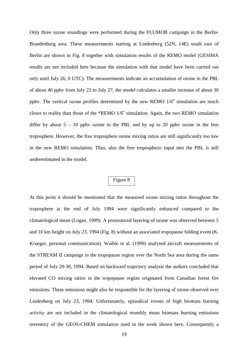
Only three ozone soundings were performed during the FLUMOB campaign in the Berlin-

Brandenburg area. These measurements starting at Lindenberg (52N, 14E) south east of

Berlin are shown in Fig. 8 together with simulation results of the REMO model (GESIMA

results are not included here because the simulation with that model have been carried out

only until July 26, 0 UTC). The measurements indicate an accumulation of ozone in the PBL

of about 40 ppbv from July 23 to July 27, the model calculates a smaller increase of about 30

ppbv. The vertical ozone profiles determined by the new REMO 1/6o simulation are much

closer to reality than those of the *REMO 1/6o simulation. Again, the two REMO simulation

differ by about 5 – 10 ppbv ozone in the PBL and by up to 20 ppbv ozone in the free

troposphere. However, the free troposphere ozone mixing ratios are still significantly too low

in the new REMO simulation. Thus, also the free tropospheric input into the PBL is still

underestimated in the model.

Figure 8

At this point it should be mentioned that the measured ozone mixing ratios throughout the

troposphere at the end of July 1994 were significantly enhanced compared to the

climatological mean (Logan, 1999). A pronounced layering of ozone was observed between 5

and 10 km height on July 23, 1994 (Fig. 8) without an associated tropopause folding event (K.

Krueger, personal communication). Waible et al. (1999) analysed aircraft measurements of

the STREAM II campaign in the tropopause region over the North Sea area during the same

period of July 20-30, 1994. Based on backward trajectory analysis the authors concluded that

elevated CO mixing ratios in the tropopause region originated from Canadian forest fire

emissions. These emissions might also be responsible for the layering of ozone observed over

Lindenberg on July 23, 1994. Unfortunately, episodical events of high biomass burning

activity are not included in the climatological monthly mean biomass burning emissions

inventory of the GEOS-CHEM simulation used in the work shown here. Consequently a

20

portion of photooxidants formation might be missing in the simulation results presented here.

Recently, activities have started to improve the timing of biomass burning emissions during

specific periods in global models using satellite observations (Duncan et al., 2002) so that a

more realistic representation of these emission can be expected in the future.

3.5. European emission reduction experiment

In this section we show results from a European wide model simulation in which

anthropogenic emissions of CO, VOC, NOx and SOx are reduced by 25 %. This reduction

corresponds approximately to the emission decrease of NO2 in Germany from 1994 to 2000

(Umweltbundesamt, 2001). The results of the sensitivity experiment, hereafter REMO-red.

1/2o are compared to the global nested REMO 1/2o simulation presented in section 3.3. The

motivation for this sensitivity experiment is to compare the effect of European wide emission

reductions with the contribution of long-range transported pollution to ozone concentrations

in surface air over Europe during summer smog conditions.

Figure 9

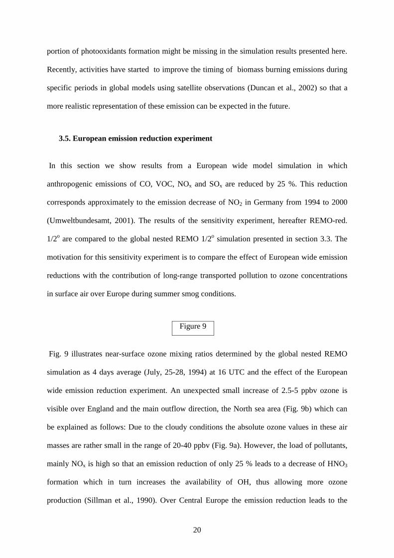
Fig. 9 illustrates near-surface ozone mixing ratios determined by the global nested REMO

simulation as 4 days average (July, 25-28, 1994) at 16 UTC and the effect of the European

wide emission reduction experiment. An unexpected small increase of 2.5-5 ppbv ozone is

visible over England and the main outflow direction, the North sea area (Fig. 9b) which can

be explained as follows: Due to the cloudy conditions the absolute ozone values in these air

masses are rather small in the range of 20-40 ppbv (Fig. 9a). However, the load of pollutants,

mainly NOx is high so that an emission reduction of only 25 % leads to a decrease of HNO3

formation which in turn increases the availability of OH, thus allowing more ozone

production (Sillman et al., 1990). Over Central Europe the emission reduction leads to the

21

expected decrease of the daily ozone maxima. The effect is stronger than 5 ppbv with

maximum values of about 10 ppbv. These values are in the same range but opposite direction

as those presented in the previous subsections related to the effect of long-range transport of

polluted air masses from outside of Europe. Thus, emissions from elsewhere (North America,

Asia) and long-range transport increase daily ozone maxima over Europe during summer

smog conditions by roughly the same amount as European emission reduction efforts decrease

daily ozone maxima.

4. Conclusions and outlook

A global to mesoscale model chain focussing on Europe, Germany and Berlin-Brandenburg

has been applied in this paper for the investigation of the effect of long-range transport of

pollution on surface air composition during a summer smog episode at the end of July 1994.

Throughout this period the global model simulation provides a first estimate of the

photochemical composition of the troposphere twice the day in a relatively coarse horizontal

resolution. Three nesting steps are performed so that the results of the respective lower

resolution model simulation are used as initial and lateral boundary data for the respective

higher resolution model simulation. Thus, we replaced one unknown contribution in the

mathematical formulation of limited area air pollution models – that is the initial and

boundary problem which is usually solved by adjusting boundary conditions within

‘acceptable’ bounds through iterative search for acceptable performance (Russel and Dennis,

2000) – by data sets produced by a global model based on physical and chemical principles.

The standard practice improves model performance without knowing the reasons whereas our

approach also offers the possibility to improve the understanding of the relevant processes

that determine tropospheric photochemistry.

22

The evaluation of model results with near-surface observations of ozone reveals a more

realistic reproduction of the variability of simulated ozone mixing ratios with increasing

horizontal resolution. Ozone mixing ratios simulated by the mesoscale models in the PBL and

the free troposphere are considerably closer to observed levels when initial and lateral

boundary conditions are taken from the global model simulation. However, the observed

unusually high mixing ratios of ozone in the free tropospheric are still underestimated in our

model simulations. A detailed analysis of the origin of ozone in the free troposphere over

Europe at the end of July 1994 is presented in a companion paper (Langmann and Bey, 2002)

to illuminate the uncertainties and the complex interactions between long-range transport of

pollutions, e.g. Canadian forest fire emissions as assumed by Waible et al. (1999), local

sources, e.g. lightning NOx production and convective mixing.

Ozone mixing ratios determined by the global model dominate the results of the higher

resolution limited area models in the free troposphere but also contribute significantly to near-

surface ozone mixing ratios. Convective mixing induced by occasionally occurring

thunderstorms couple the air masses of the free troposphere and the PBL over Europe. It is

shown that ozone from the free troposphere is injected into the PBL contributing an amount of

at least 5-10 ppbv to maximum near-surface ozone mixing ratios during the summer smog

episode under investigation. It should be noted, however, that the contribution of long-range

transported pollution to ozone concentrations in surface air calculated for that period might

not be representative of typical situations because of especially high convective activity

which contributes significantly to vertical transfer between the PBL and the free troposphere.

Further work is needed to evaluate such numbers on a climatological base.

When reducing anthropogenic emissions by 25 % (corresponding approximately to the

emission reduction in Germany from 1994 - 2000) in a European wide model simulation we

23

receive again a modification of 5-10 ppbv in maximum near-surface ozone over Central

Europe, a decrease in this case. From these results we conclude that intercontinental transport

of pollution can obscure the results of local efforts to reduce critical exposure levels of ozone

during summer smog conditions. European pollution might also be reduced by decreasing

emissions elsewhere due to the decreasing contribution to the long range transport of

pollution. Other aspects that affect the long range transport of pollution and its impact on

European pollution levels are modifications in large scale dynamics. For example, Li et al.

(2002) found a high correlation (r = 0.57) between the North Atlantic Oscillation (NAO)

index and ‘North American ozone’ at Mace Head, a remote site at the Atlantic coast of Ireland

for the period 1993 – 1997. A decline in the NAO index would reduce transatlantic transport

of American pollution to Europe. Although in Osborn et al. (1999) a significant decline in the

NAO index is predicted using a general circulation model with anthropogenic forcing from

greenhouse gases and sulphate aerosols, a new manuscript in preparation by Osborn (2002)

using a pattern-based measure of the NAO concludes the opposite – namely a weak increase

in the NAO. This revised result concerning NAO could lead to an increase of transatlantic

transport of American pollution to Europe emphasising that global restrictions of

anthropogenic CO, VOC and NOx emissions are necessary to reduce and control the

formation of photooxidants.

Acknowledgements

The authors would like to acknowledge all the scientists and institutes involved in the

development of the numerical models applied in this paper and those who made their data

available, and thanks to Christiane Textor and Martin Schultz from the MPI for Meteorology

and the two anonymous reviewers for their valuable comments on the manuscript.

24

References

Allen, D. J., R. B. Rood, A. M. Thompson, and R. D. Hidson, Three-dimensional radon222

calculations using assimilated data and a convective mixing algorithm, J. Geophy. Res.,

101, 6871-6881, 1996a.

Allen, D. J., P. Kasibhatla, A. M. Thompson, R. B. Rood, B. G. Doddridge, K. E. Pickering,

R. D. Hudson, and S. J. Lin, Transport induced interannual variability of carbon

monoxide using a chemistry and transport model, J. Geophy. Res., 101, 28,655-28,670,

1996b.

Bauer, S. E.: Photochemical smog in Berlin-Brandenburg: An investigation with the

atmosphere-chemistry model GESIMA, Ph.D. Thesis, Examination Report No. 81,

Max-Planck-Institute for Meteorology, Hamburg, Germany, 2000.

Bauer, S. E. and B. Langmann, An atmosphere-chemistry model on the meso-γ scale: Model

description and evaluation, Atmos. Environ., in press, 2002a.

Bauer, S. E. and B. Langmann, Analysis of a summer smog episode in the Berlin-

Brandenburg region with a nested atmosphere – chemistry model, Atmos. Chem. Phys.,

submitted, 2002b.

Berliner Wetterkarte, available from the Institute for Meteorology, University of Berlin, Carl-

Heinrich-Becker-Weg 6-10, 12165 Berlin, Germany, July 1994.

Bey, I., D. J. Jacob, R. M. Yantosca, J. A. Logan, B. D. Field, A. M. Fiore, Q. Li, H. Y. Liu,

L. J. Mickley, and M. G. Schultz, Global modeling of tropospheric chemistry with

assimilated meteorology: Model description and evaluation, J. Geophy. Res., 23,073-

23,096, 2001.

Chameides, W. L., R. W. Lindsay, J. Richardson, and C. S. Chiang, The role of biogenic

hydrocarbons in urban photochemical smog: Atlanta as a case study, Science, 241,

1473-1475, 1988.

Chang, J. S., R. A. Brost, S. A. Isaksen, S. Madronich, P. Middleton, W. R. Stockwell and C.

J. Walcek, A three dimensional Eulerian acid deposition model: physical concepts and

formulation, J. Geophys. Res., 92, 14,681-14,700, 1987.

25

Duncan B. N., R. V. Martin, A. C. Staudt, R. Yevich and J. A. Logan: Interannual and

Seasonal Variability of Biomass Burning Emissions constrained by Satellite

Observations, J. Geophys. Res., submitted, 2002.

Fiore, A. M., D. J. Jacob, I. Bey, R. M. Yantosca and B. D. Field, Background ozone over the

United States in summer: origin and contribution to pollution episodes, J. Geophys.

Res., in press, 2002.

Forster, C., P. James, G. Wotowa, U. Wandinger, I. Mattis, D. Alshausen, P. Simmonds, S.

O’Doherty, S. G. Jennings, C. Kleefeld, J. Schneider, T. Trickl, S. Kreipl, H. Jaeger and

A. Stohl, Transport of boreal forest fire emissions from Canada to Europe, J. Geophys.

Res., 106, 22,887-22,906, 2001.

Guenther, A. B., R. K. Monson and R. Fall, Isoprene and monoterpene emission rate

variability: Observations with eucalyptus and emission rate algorithm development, J.

Geophys. Res., 96, 10,799-10,808, 1991.

Guenther, A. B., P. R. Zimmermann, P. C. Harley, R. K. Monson and R. Fall, Isoprene and

monoterpene emission rate variability: Model evaluation and sensitivity analysis, J.

Geophys. Res., 98, 12,609-12,617, 1993.

Guenther, A., C. N. Hewitt, D. Erickson, R. Fall, C. Geron, T. Graedel, P. Harley, L. Klinger,

M. Lerdau, W. A. Mckay, T. Pierce, B. Scholes, R. Steinbrecher, R. Tallamraju, J.

Taylor, and P. Zimmerman, A global model of natural volatile organic compound

emissions, J. Geophy. Res., 100, 8873-8892, 1995.

Horowitz, L. W., J. Liang,, G. M. Gardner, and D. J. Jacob, Export of reactive nitrogen from

North America during summertime: Sensitivity to hydrocarbon chemistry, J. Geophy.

Res., 103, 13,451-13,476, 1998.

Jacob, D. J., J. A. Logan, and P. P. Murti, Effect of rising Asian emissions on surface ozone in

the United States, Geophys. Res. Lett., 26, 2175-2178, 1999.

Jaffe, D., T. Anderson, D. Covert, R. Kotchenruther, B. Trost, J. Danielson, W. Simpson, T.

Berntsen, S. Karlsdottir, D. Blake, J. Harris, G. Carmichael, and I. Uno, Transport of

Asian air pollution to North America, Geophys. Res. Lett., 26, 711-714, 1999.

Kapitza, H. and D. Eppel, The non-hydrostatic mesoscale model GESIMA. Part I: Dynamical

equations and tests, Contr. Atmosph. Phys., 65, 129-146, 1992.

Langmann, B., Numerical modelling of regional scale transport and photochemistry directly

together with meteorological processes, Atmos. Environ., 34, 3585-3598, 2000.

Langmann, B. and S. E. Bauer, On the importance of reliable background concentrations of

ozone for regional scale photochemical modelling, J. Atmos. Chem, in print, 2002.

26

Langmann, B. and I. Bey, The influence of the global photochemical composition of the

troposphere on European summer smog, Part II: Impact of lightning and North

American emissions, in preparation, 2002.

Li, Q., D. J. Jacob, I. Bey, R. M. Yantosca, B. D. Field, J. A. Logan, A. M. Fiore, R. V.

Martin, and B. N. Duncan, Sources of ozone over the North Atlantic and trans-Atlantic

transport of pollution: A global model perspective, IGAC Newsletter, 24, 12-17, 2001.

Li Q., D. J. Jacob, I. Bey, P. I. Palmer, B. N. Duncan, B. D. Field, R. V. Martin, A. M. Fiore,

R. M. Yantosca, D. D. Parrish, P. G. Simmonds, and S. J. Oltmans, Transatlantic

transport of pollution and its effects on surface ozone in Europe and North America, J.

Geophys. Res., in press, 2002.

Lin, S.-J. and R. B. Rood, Multidimensional flux form semi-Lagrangian transport schemes,

Mon. Wea. Rev., 124, 2046-2070, 1996.

Logan, J. A., An analysis of ozonesonde data for the troposphere: Recommendations for

testing 3-D models and development of a gridded climatology for tropospheric ozone, J.

Geophy. Res., 104, 16,115-16,149, 1999.

Madronich, S., Photodissociation in the atmosphere, I. Actinic flux and the effect of ground

reflections and clouds, J. Geophys. Res., 92, 9740-9752, 1987.

Majewski, D., Balanced initial and boundary values for a limited area model, Contr. Atmosph.

Phys., 58, 147-159, 1985.

Majewski, D., The Europa Modell of the Deutscher Wetterdienst, Seminar proceedings

ECMWF, 2, pp. 147-191, 1991.

Mellor, B. and T. Yamada, A hierachy of turbulence closure models for planetary boundary

layers, J. Atmos. Sci., 31, 1791-1806, 1974.

Mesinger, F. and A. Arakawa, Numerical methods used in atmospheric models, GARP

Publications Series, No. 17, pp. 1-64, WMO.

Osborn, T. J., K. R. Briffa, S. F. B. Tett, P. D. Jones and R. M. Trigo, Evaluation of the North

Atlantic Oscillation as simulated by a coupled climate model, Clim. Dyn., 15, 685-702,

1999.

Osborn, T. J., The winter North Atlantic Oscillation: the roles of internal variability and

greenhouse gas forcing, in preparation, 2002.

Parrish, D. D., J. S. Holloway, M. Trainer, P. C. Murphy, G. L. Forbes and F. C. Fehsenfeld,

Export of North American Ozone Pollution to the North Atlantic Ocean, Science, 259,

1436-1438, 1993.

27

Pleim, J. E., J. S. Chang, and K. Zhang, A nested grid mesoscale atmospheric chemistry

model, J. Geophys. Res., 96, 3065-3084, 1991.

Roelofs, G. J. and J. Lelieveld, Model study of the influence of cross-tropopause O3 transports

on tropospheric O3 levels, Tellus, 49B, 38-55, 1997.

Russell, A. and R. Dennis, NASTRO critical review of photochemical models and modelling,

Atmos. Environ., 34, 2283-2324, 2000.

Sillman, S., J. A. Logan and S. C. Wolfsy, The sensitivity of ozone to nitrogen oxides and

hydrocarbons in regional ozone episodes, J. Geophys. Res., 95, 1837-1851, 1990.

Simpson, D., W. Winiwarter, G. Boerjesson, S. Cinderby, A. Ferreiro, A. Guenther, C. N.

Hewitt, R. Janson, M. A. K. Khalil, S. Owen, T. E. Pierce, H. Puxbaum, M. Shearer, U.

Skiba, R. Steinbrecher, L. Tarrason, and M. G. Oequist, Inventorying emissions from

nature in Europe, J. Geophys. Res., 104, 8113-8152, 1999.

Singh, H. B. and D. J. Jacob, Future directions: Satellite observations of tropospheric

chemistry, Atmos. Environ., 34, 4399-4401, 2000.

Smolarkiewitz, P. K., A simple positive definite advection scheme with small implicit

diffusion, Mon. Wea. Rev., 111, 479-486, 1983.

Smolarkiewitz, P. K., A fully multidimensional positive definite advection transport algorithm

with small implicit diffusion, J. Comp. Phys., 54, 325-362, 1984.

Stockwell, W. R., P. Middleton, J. S. Chang and X. Tang, The second generation regional

acid deposition model: Chemical mechanism for regional air quality modelling, J.

Geophys. Res., 95, 16,343-16,367, 1990.

Stohl, A. and T. Trickl, A textbook example of long-range transport: Simultaneous

observation of ozone maxima of stratospheric and North American origin in the free

troposphere over Europe, J. Geophys. Res., 104, 30,445-30,462, 1999.

Tiedtke, M., A comprehensive mass flux scheme for cumulus parameterization in large-scale

models, Mon. Wea. Rev., 117, 1778-1800, 1989.

Umweltbundesamt, Luft kennt keine Grenzen, 6. Auflage, Berlin, Germany, 2001. (available

from http://www.umweltbundesamt.de )

Walcek, C. J. and G. R. Taylor, A theoretical method for computing vertical distributions of

acidity and sulfate production within cumulus clouds, J. Atmos. Sci., 43, 339-355, 1986.

Wang, Y., D. J. Jacob, and J. A. Logan, Global simulation of tropospheric O3-NOx-

hydrocarbon chemistry, 1. Formulation, J. Geophys. Res., 103, 10,713-10,725, 1998.

Waibel, A. E., H. Fischer, F. G. Wienhold, P. C. Siegmund, B. Lee, J. Stroem, J. Lelieveld,

and P. J. Crutzen, Highly elevated carbon monoxide concentrations in the upper

28

troposphere and lowermost stratosphere at northern midlatitudes during the STREAM II

campaign in 1994, Chemosphere: Global Change Science, 1, 233-248, 1999.

Wesley, M. L., Parameterization of surface resistances to gaseous dry deposition in regional-

scale numerical models, Atmos. Environ., 23, 1293-1304, 1989.

Figure captions Fig. 1: The global to mesoscale model chain. Surface orographie and a map of the Berlin-

Brandenburg area are shown.

Fig. 2: Vertical distribution of 12 UTC ozone in ppbv at [20N, 20W], [50N, 20W] and [80N,

20W] during July, 20 – 30, 1994 as determined by the global GEOS-CHEM model. For

clarity reasons the data are shown only in two day intervals.

Fig. 3: Modelled vertical ozone distribution in ppbv up to approximately 13 km height during

July, 20, 12 UTC – 30, 12 UTC, 1994, averaged over 4 European regions following the

locations of stations indicated in Appendix A: 4 Spanish station (first row), 10 Alpine stations

(second row), 24 German stations (third row) and 12 British stations (fourth row). Left

column: GEOS-CHEM simulation, mid column: REMO 1/2ο simulation, right column:

*REMO 1/2ο.

Fig. 4: Time series of the measured and modelled near-surface ozone mixing ratios during

July, 20 – 30, 1994 averaged over 4 European regions following the locations of stations

indicated in Appendix A.

Fig. 5: Maximum near-surface ozone mixing ratios (hourly data from 12-16 UTC from all

stations mentioned in Appendix A) as determined by the global nested REMO 1/2o simulation

and the *REMO 1/2o simulation versus observations for the period July 22-30, 1994. The

dashed lines indicate factor of 2 deviations from perfect agreement.

Fig. 6: Near-surface ozone mixing ratios at 27 sites in the Berlin-Brandenburg area:

Measurements and model results during July 22-25, 1994. For the GESIMA calculations the

area of Berlin-Brandenburg is represented by 50 x 50 grid points. Approximately 11 x 11 grid

points cover the area in the REMO 1/6ο simulation and only 4 x 4 grid points in the REMO

1/2ο simulation.

29

Fig. 7: Aircraft measurements a) during the morning and b) during the afternoon hours of July

25, 1994 compared with model results. GESIMA represents global to mesoscale model chain

results, *GESIMA represents mesoscale model chain results.

Fig. 8: Ozone sonde observations at Lindenberg (52N, 14E) and model results from REMO.

Fig. 9: a) Near-surface ozone mixing ratios as determined by the global nested REMO 1/2ο

simulation as 4 days average (July, 25-28, 1994) at 16 UTC together with b) the difference:

REMO 1/2ο minus REMO-red. 1/2ο simulation results which represent the European wide

emission reduction effect.

30

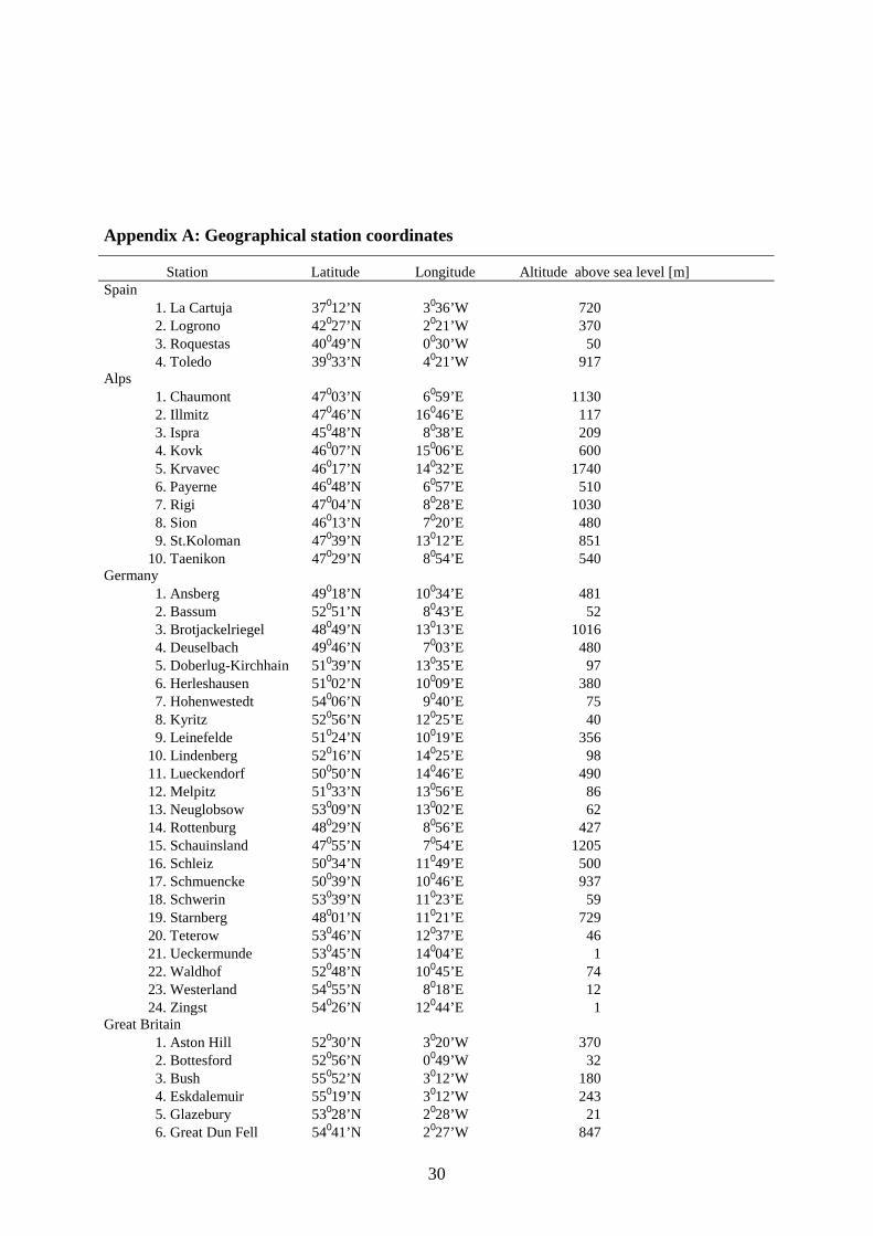
Appendix A: Geographical station coordinates

Station Latitude Longitude Altitude above sea level [m] Spain

1. La Cartuja 37012’N 3036’W 720 2. Logrono 42027’N 2021’W 370 3. Roquestas 40049’N 0030’W 50 4. Toledo 39033’N 4021’W 917

Alps

1. Chaumont 47003’N 6059’E 1130 2. Illmitz 47046’N 16046’E 117 3. Ispra 45048’N 8038’E 209 4. Kovk 46007’N 15006’E 600 5. Krvavec 46017’N 14032’E 1740 6. Payerne 46048’N 6057’E 510 7. Rigi 47004’N 8028’E 1030 8. Sion 46013’N 7020’E 480 9. St.Koloman 47039’N 13012’E 851 10. Taenikon 47029’N 8054’E 540

Germany

1. Ansberg 49018’N 10034’E 481 2. Bassum 52051’N 8043’E 52 3. Brotjackelriegel 48049’N 13013’E 1016 4. Deuselbach 49046’N 7003’E 480 5. Doberlug-Kirchhain 51039’N 13035’E 97 6. Herleshausen 51002’N 10009’E 380 7. Hohenwestedt 54006’N 9040’E 75 8. Kyritz 52056’N 12025’E 40 9. Leinefelde 51024’N 10019’E 356 10. Lindenberg 52016’N 14025’E 98 11. Lueckendorf 50050’N 14046’E 490 12. Melpitz 51033’N 13056’E 86 13. Neuglobsow 53009’N 13002’E 62 14. Rottenburg 48029’N 8056’E 427 15. Schauinsland 47055’N 7054’E 1205 16. Schleiz 50034’N 11049’E 500 17. Schmuencke 50039’N 10046’E 937 18. Schwerin 53039’N 11023’E 59 19. Starnberg 48001’N 11021’E 729 20. Teterow 53046’N 12037’E 46 21. Ueckermunde 53045’N 14004’E 1 22. Waldhof 52048’N 10045’E 74 23. Westerland 54055’N 8018’E 12 24. Zingst 54026’N 12044’E 1

Great Britain

1. Aston Hill 52030’N 3020’W 370 2. Bottesford 52056’N 0049’W 32 3. Bush 55052’N 3012’W 180 4. Eskdalemuir 55019’N 3012’W 243 5. Glazebury 53028’N 2028’W 21 6. Great Dun Fell 54041’N 2027’W 847

31

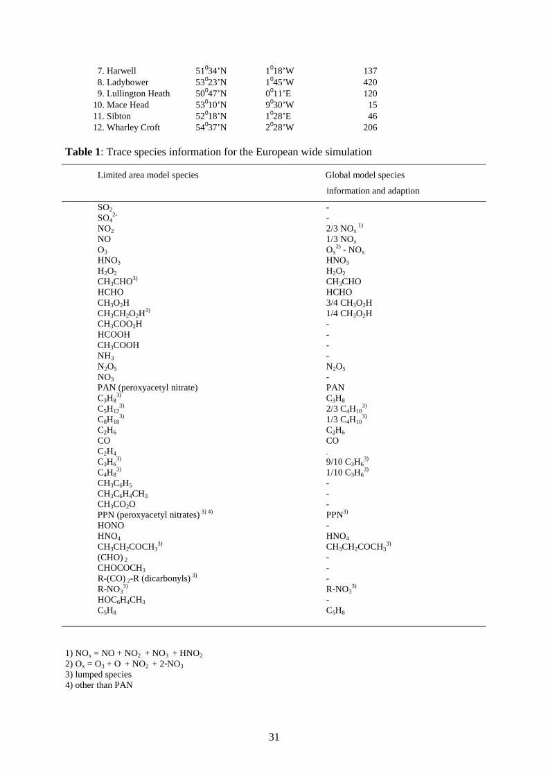
7. Harwell 51034’N 1018’W 137 8. Ladybower 53023’N 1045’W 420 9. Lullington Heath 50047’N 0011’E 120 10. Mace Head 53010’N 9030’W 15 11. Sibton 52018’N 1028’E 46 12. Wharley Croft 54037’N 2028’W 206 Table 1: Trace species information for the European wide simulation

Limited area model species Global model species

information and adaption

SO2 - SO4

2- - NO2 2/3 NOx

1) NO 1/3 NOx O3 Ox

2) - NOx HNO3 HNO3 H2O2 H2O2 CH3CHO3) CH3CHO HCHO HCHO CH3O2H 3/4 CH3O2H CH3CH2O2H

3) 1/4 CH3O2H CH3COO2H - HCOOH - CH3COOH - NH3 - N2O5 N2O5 NO3 - PAN (peroxyacetyl nitrate) PAN C3H8

3) C3H8 C5H12

3) 2/3 C4H103)

C8H183) 1/3 C4H10

3) C2H6 C2H6 CO CO C2H4 - C3H6

3) 9/10 C3H63)

C4H83) 1/10 C3H6

3) CH3C6H5 - CH3C6H4CH3 - CH3CO2O - PPN (peroxyacetyl nitrates) 3) 4) PPN3) HONO - HNO4 HNO4 CH3CH2COCH3

3) CH3CH2COCH33)

(CHO) 2 - CHOCOCH3 - R-(CO) 2-R (dicarbonyls) 3) - R-NO3

3) R-NO33)

HOC6H4CH3 - C5H8 C5H8 1) NOx = NO + NO2 + NO3 + HNO2 2) Ox = O3 + O + NO2 + 2*NO3 3) lumped species 4) other than PAN