THE INFLUENCE OF IRRIGATION WITHGYPSIFEROUS MINE WATER ON SOIL PROPERTIES

AND DRAINAGE WATER

JG Annandale • NZ JovanovicAS Claassens

WRC Report No. 858/1/02

Water Research Commission

Disclaimer

This report emanates from a project financed by the Water Research Commission (WRC) andis approved for publication. Approval does not signify that the contents necessarily reflect theviews and policies of the WRC or the members of the project steering committee, nor doesmention of trade names or commercial products constitute endorsement or recommendation foruse.

Printed by Silowa Printers

EXECUTIVE SUMMARYIntroduction

The mining industry is one of the most important in South Africa, both from the point of view ofgross national product and job creation. In the mining of mineral resources, pollution problemsare created with adverse effects on the already scarce water resources. The type of wastewater emanating from mines depends largely on the geological properties of the coal, gold oreand other geological material with which waters come into contact. The concentrations of saltsand other constituents frequently render this water unsuitable for direct discharge to the riversystems except in periods of high rainfall when an adequate dilution capacity is present andcontrolled release is allowed. Gypsiferous mine water can either be regarded as one of mining'sgreatest problems, or as a potential asset. Large amounts of waste water could possibly bemade available to the farming community and utilized for irrigation of high-potential soils in thecoalfields of Mpumalanga Province, where water resources for irrigation are already underpressure. Concentrating the gypsiferous soil solution through evapotranspiration, therebyprecipitating gypsum in the profile and removing this salt from the water system, could also limitenvironmental pollution. Therefore, the use of gypsiferous mine water for the irrigation ofagricultural crops is a promising technology that could add value through agriculture productionand utilize effluent mine drainage.

Objectives of the project

In this project, the general objective was to ascertain whether gypsiferous mine water can beused on a sustainable basis for irrigation of crops and/or amelioration of acidic soils. This wasachieved by addressing the following secondary aims:

1) Assess the feasibility of managing irrigation with gypsiferous mine water at semi-operational scale in such a way that surface and groundwater contamination isreduced, while soil suitability and crop production are maintained.

2) Evaluate the effect of irrigation with gypsiferous water on the following:

2.1) Yield and plant nutritional effects on a selection of agronomic crops thatcan be grown in the area.

2.2) Gypsum precipitation and immobilization of other chemical constituents inthe soil.

2.3) Effects of gypsum precipitation and salt accumulation on soilcharacteristics.

2.4) Depth of salinization of soil over time.2.5) Quality and quantity of drainage water.2.6) Impact of seasonal and annual rainfall on soil and drainage water

characteristics.2.7) The ameliorating effect of gypsiferous water on acidic soils.

3) Develop predictive models for salt and water budgets for soil under irrigation withgypsum rich mine water.

4) Evaluate and refine these models practically over a (three year) period with summerand winter crops.

i l l

5) Model long-term salt and water budgets for different scenarios.

6) Provide inputs to any associated groundwater studies.

Following the acceptance of the project proposal, it was realized that investigations into theimpact of irrigation on the groundwater regime were also necessary. The following objective wastherefore added:

7) Investigate the extent of groundwater contamination through:

7.1) A complete description of the groundwater regimes in areas to beirrigated, detailing the geohydrology as well as groundwater qualitybefore, during and after irrigation.

7.2) Interpretation of data through the establishment of an expert system andgeohydrological modelling to facilitate the prediction of the medium- andlong-term impacts on both local and regional scales.

Materials and methods

The objectives have been tackled using a multi-disciplinary approach, where various aspects ofthe impact of irrigation with gypsiferous mine water were investigated.

A field trial was set up at Kleinkopje Colliery from the summer season of 1997 until andincluding the winter of 2000, where several crops were irrigated with centre pivots using twomine waters (Jacuzzi and Tweefontein). Jacuzzi water is pumped from underground into aholding dam, whilst Tweefontein Pan holds water pumped from the active opencast pit. PivotsMajor and Fourth were set up on virgin (unmined) land, whilst pivots Tweefontein and Jacuzziwere set up on rehabilitated land. A summary of water sources and pivots is presented below.

Water source

Jacuzzi Dam

Tweefontein Pan

From 1997 to 1999Major

JacuzziTweefontein

From 1999 to 2000Major

TweefonteinFourth

Pivot No.# 1#2# 3# 4

LandVirgin

RehabilitatedRehabilitated

Virgin

Three different irrigation management practices were adopted for each pivot: irrigation with aleaching fraction, irrigation up to field capacity and deficit irrigation (room for rain). Two farmingcompanies were involved in commercial crop production on the pivot sites, namely, Amfarmsfrom 1997 to 1999, and Smith Bros, from 1999 to 2000.

The following measurements were made during the course of the field trial:

i)

ii)

Growth and yield of sugarbeans, maize and wheat were monitored to determinewhether these crops can be commercially produced under irrigation with mine water,as well as to provide data sets for validation of the crop growth subroutine of theSWB model. Several alternative cropping systems were also tested.Plant samples were collected at different growth stages for laboratory analysts toidentify and correct possible plant nutrient deficiencies through fertilization. Nutrientdeficiencies could occur due to excess gypsum and other salts in irrigation water.

iii) Atmospheric measurements were made using an automatic weather station toprovide data sets for validation of the SWB model.

iv) Soil materials were described in terms of their physical properties by determiningbulk density, water retention, hydraulic conductivity and the solute transportcharacteristics of dispersion, adsorption and rate dependant transfers. This wasdone to describe the general behaviour of the water and salt fluxes in the profiles, todetermine initial inputs for the SWB model and to evaluate specific phenomena in theporous media, such as changes to pore structure due to gypsum precipitation.

v) Soil water and salt balance data were collected using intensive monitoring stationsfor each pivot and irrigation treatment, to determine crop water use and soil salinity,as well as to provide data sets for validation of the water and salt redistributionsubroutines of the SWB model.

The equipment used to measure the soil water balance included:Tipping bucket rain gauges for measurement of irrigation water appliedand rainfall.Tensiometers and heat dissipation sensors for measurement of soilmatric potential at different depths in the soil profile.

- Neutron water meter, CS-615 soil water reflectometers and time domainreflectometry (TDR) for measurement of volumetric soil water content atdifferent depths in the soil profile.

The equipment used to measure the salt balance included:Ceramic cup soil water samplers used to extract soil water forlaboratory analysis from different depths in the soil profile.TDR for measurement of bulk soil electrical conductivity.Electromagnetic induction was used to determine soil salinity over theentire field on a grid basis. This was done to get an idea of spatialvariability of soil salinity.Laboratory analyses of irrigation water were also carried out todetermine its quality. Irrigation water samples were collected with plasticbottles at the water source and from pivot nozzles.

vi) Soil chemical analyses were carried out at regular intervals (every season) todetermine possible changes in soil chemical properties due to irrigation with minewater, as well as the amount of gypsum precipitated in the soil profile.

vii) Deep soil sampling was carried out in June 2000 for chemical analyses in thelaboratory, in order to explore whether any salt breakthrough originating fromirrigation could be identified deeper in the soil profile.

viii) Runoff volumes and quality were measured at crump weirs built at the lowest pointsbelow pivots Major and Tweefontein.

ix) Groundwater quality was monitored to determine possible breakthrough of saltsoriginating from irrigation at pivot Major. For this purpose, nine boreholes wereinstalled at specific localities where they were most likely to intersect pollutedgroundwater. Water quality and water levels were the key parameters measured.During the installation of the boreholes, the following additional features were alsonoted and measured: geology; water strikes and yields; the hydraulic conductivity ofthe strata through packer and/or pumping tests; the installation of piezometer tubesto exclude cross contamination from surface water to the groundwater.

Plant nutritional aspects were investigated in a glasshouse pot trial. The aims were to determinewhether plants can grow and produce acceptable yields under irrigation with gypsiferous minewater, and to recommend optimal nutrient management. This work was done becausenutritional problems could materialize under irrigation with water rich in Ca, Mg and SO4 due tocompetition for nutrient uptake. Nutritional imbalances could cause both reduced economicreturn from crop production and reduced mine water consumption through crop transpiration.

A decision was taken to investigate the possible adverse effects of mine water on herbicideactivity after maize crops were damaged on all three pivots in the beginning of the 1999/00season, through the inadvertent application of excess herbicide. This resulted in significant yieldlosses. The objectives of this preliminary investigation were to determine the influence of minewater on the three important performance criteria for herbicides: weed control efficacy, herbicideselectivity, as well as herbicide persistence and mobility in soil (incorporating risks ofenvironmental pollution). For this purpose, chemical analyses of selected herbicides in agypsiferous tank mixture were done by gas chromatography analysis. In a parallel investigation,bioassays were conducted in a greenhouse in order to assess whether the biological activity ofthe selected herbicides is affected by the presence of gypsum in soil.

The purpose of the Kleinkopje field trial was to investigate commercial feasibility of cropproduction and environmental impact under irrigation with mine water in the short term (threeyears). However, the problem of saline water management also has long-term implications.Long-term changes in soil chemical and physical properties can be measured, but the executionof long-term experiments monitoring slow environmental processes can be prohibitivelyexpensive and it is not always possible to wait for the outcome of such experiments. For thisreason, it was necessary to adapt the SWB model for long-term (50 years) predictions of soilwater and salt balance under irrigation with mine water. In order to be confident of the long-termpredictions of SWB, the model had to be refined and validated using atmospheric, soil and cropdata collected in the field trial.

It was not possible to investigate all cropping systems and management options that could besuitable for the utilization of gypsiferous mine water at the Kleinkopje irrigation sites. A scenariostudy was therefore carried out using the SWB model in order to recommend other suitablecropping systems and agricultural management practices for the area in the vicinity ofKleinkopje Colliery. A simple economic analysis was also required in order to recommend themost profitable and environmentally sustainable cropping and irrigation water managementsystem.

In order to investigate the extent of groundwater contamination in the long term, SWB outputwas used by a finite element groundwater model. The purpose was to predict the groundwaterflow and potential pollution migration for a case study at pivot Major.

General findings

In the field trial at Kleinkopje Colliery, crop yields were generally high and the farmingcompanies were keen to participate in the project. The study has shown that crops can besuccessfully grown under irrigation with gypsiferous mine water on a commercial basis.

Yield losses were experienced on two pivots on rehabilitated land (Jacuzzi and Tweefontein)due to waterlogging during the summer seasons, even after levelling work had been carried outand waterways constructed. This was probably due to subsurface drainage from higher areas

VI

and accumulation of water in lower areas through lateral movement of water above the spoillayer.

No symptoms of foliar injury due to sprinkler irrigation with gypsiferous water were noted for anyof the crops. Visual observation and laboratory analyses of plant samples indicated that nospecific symptoms of nutrient deficiency or toxicity occurred due to excess gypsum in irrigationwater.

Soil chemical analyses were carried out during the field trial to determine general trends in soilchemical properties. Soil pH(H2O) generally showed a slight increasing tendency at all pivotsover the study period. Soil salinity generally showed a tendency to increase over time, butfluctuated depending on seasonal rainfall as well as the irrigation and rainfall events prior to soilsampling.

The results of the spatial variability study indicated that there is a tendency for salinity levels tobe higher in the central region of each pivot. This is believed to be due to the larger quantities ofsaline irrigation water applied in these zones during the course of the experiment. Major pivotshowed an accumulation of salts in the lower south-eastern region, in clayey soils in thedrainage line. This appears to reflect the direction of water movement down the slope, and theimpedance to water and salt movement in the heavy soils.

Deep soil samples were collected in June 2000 for laboratory analyses. It was observed that atpivot Major and Tweefontein, most soluble salts were confined to the upper 1 m, probably dueto the presence of a plinthic and spoil layer respectively, which were limiting free drainage. Atpivot Fourth, in the absence of a layer preventing deep percolation, there was a more uniformdistribution of salts in the soil profile, with a slight peak between 1.5 and 2 m down in the profileindicating leaching of salts below the root-zone, even though this field had not been irrigated foras long as pivot Major. An attempt to measure gypsum precipitated in the soil profile was alsomade on deep soil samples. It was, however, clear from the results obtained that a reliablemethod to measure gypsum precipitation still needs to be developed, as much higher values ofmeasured precipitated gypsum were obtained than the amount of salts added through irrigation,based on measured irrigation water quality and amount.

Irrigation water quality analyses indicated that Jacuzzi and Tweefontein waters were similar.Seasonal fluctuations in irrigation water salinity can be expected depending on seasonal rainfall.

Runoff volumes and quality data collected at the weirs from November 1999 to April 2000,indicated that less than 2% of the salts added since the beginning of the trial were lost from theirrigated fields through runoff. More runoff was recorded at pivot Tweefontein compared to pivotMajor, due to the restricted soil depth and steep slopes of the rehabilitated land. Due toimpervious soil layers at pivots Major and Tweefontein, it is likely that runoff and salts in runoffcould have mainly originated from lateral movement of soil water.

Salt migration through soil and aquifers is a slow process. After more than three years ofirrigation, there was still no conclusive evidence that saline irrigation water had reached theaquifer below the irrigation site at pivot Major. This is in spite of the fact that groundwater levelsare within 1 - 3 m from the surface. A slight rise in nitrate concentrations was observed at twoboreholes. This was derived from fertilizer application. At five of the boreholes, a small increasein calcium, magnesium and sulphate levels was observed.

Vll

Data collected in the field trial were compared to model simulations in order to validate the SWBmodel. The model predicted crop growth, water and salt redistribution generally quite well. Fieldmeasurements and model predictions were used to compile soil water and salt balances for allseasons and treatments of the field trial. These accurate predictions of the water and saltbalance with SWB in the short term gave confidence that the model can be applied for long-termpredictions.

Fifty-year scenario simulations were then carried out with SWB. Multiple Criteria Decision-Making (MCDM) techniques were used to advise Kleinkopje Colliery's management on the besteconomically and environmentally sustainable cropping system for irrigation with gypsiferousmine water. From this scenario modelling study, it was clear that perennial pastures have thebiggest year round green canopy, and will therefore use the most water and precipitate the mostsalts. They will also be the most profitable cropping systems, provided that the companymanaging the irrigation pivots is geared to animal production systems. These systems,however, tend to be more labour intensive and are therefore often not preferred. Cash cropsystems lend themselves to mechanization and are therefore often preferred by bigger farmingcompanies. Irrigation management practices also contributed to the sustainability of the system.Simulated yields were the highest for the leaching fraction strategy. However, with this strategy,more salts were leached (64% of the applied salts) compared to the "room for rain" strategywhere only 53% of applied salts were leached.

The output of the SWB model was used as input into a groundwater model in order to predictthe long-term effects of irrigation with gypsiferous mine water on groundwater for a case studyat pivot Major. Irrigation treatments were simulated with SWB for the period of the field trial(from December 1997 to November 2000) followed by 50 years of scenario simulation. Twosimulations were done with the groundwater model. The first simulation was that of potentialpollution dispersion from the irrigation area. The second simulation included the "dirty" Jacuzziwater controlled release dam. The results of modelling potential pollution migration through theaquifer suggested migration to the South-West, eventually to emanate in the stream at aconcentration of about 30% of that in the aquifer below the irrigated site. This drop in salt levelswas ascribed to dilution by rainwater infiltration and the dispersive characteristics of the aquifer.

Technical findings

In the field trial, several crops were irrigated with gypsiferous mine water. Although comparableyield data for crops irrigated with good quality water are not available, the yield of sugar beansunder irrigation with mine water on virgin soil (3.23 Mg ha'1) was comparable to yields registeredin the area, and definitely higher than under dry land conditions (1.12 Mg ha'1). Yields of sugarbeans on rehabilitated land (between 1.23 and 1.37 Mg ha"1) were, however, low compared tovirgin iand, likely due to late planting dates, hail damage, soil compaction, low soil pH andnutritional deficiencies. Excellent yields of wheat (between 5.04 and 8.08 Mg ha"1) wereobtained on both virgin and rehabilitated land. The yield of the short-season cultivar of maizewas also good on virgin land (7.83 Mg ha'1, 1998/99 season). An excess of herbicide mistakenlyapplied to all three pivots by the farming company, caused severe reductions in maize yields insummer 1999/2000. In October 2000, a hailstorm completely wiped out the wheat crops atpivots Fourth and Tweefontein. The estimated loss in crop at pivot Major was 40%. Thepotential yield at all three pivots was 8 Mg ha"1.

Soil chemical analyses indicated that the soil saturated electrical conductivity andconcentrations of soluble Ca2+, Mg2+ and SO4

2" generally increased over time at all four pivotsites. This was due to the relatively high concentrations of these ions in irrigation water. The

Vl l l

values of soluble K+ did not show any particular trend and they were lower by one order ofmagnitude than the other cations, as the irrigation water had a low concentration of K+.Exchangeable Ca2+ and Mg2+ increased with time, whilst K+ decreased at all four pivot sites.This indicated that Ca2+ and, to a certain extent Mg2*, replaced K+ on the soil adsorptivecomplex. Very low values of exchangeable Na+ were measured during the course of the trial.

The results of the analyses of soil water extracted with ceramic cup soil water samplers,indicated that soil salinity is a very dynamic variable as it depends on many factors, mainlyrainfall, irrigation amounts and evapotranspiration. The data generally indicated higher soilsalinity in the topsoil layers compared to deeper layers. This proves that salt, in particulargypsum, accumulated and precipitated where the rooting system is most dense.

Several methods to measure gypsum precipitated in the soil were considered. The AdaptedDilution Method was eventually selected and applied. It appeared, however, from the resultsobtained, that this methodology is not suitable, as much higher values of measured precipitatedgypsum were obtained compared to the amount of salts added through irrigation.

Plant nutritional aspects were investigated in a glasshouse pot trial. Salinity decreased thebiomass production of wheat, mainly due to interactions of Mg and Mn with the uptake of Feand K. Decreases in yield were also associated with significant increases in plantconcentrations of SO4 and Mg. The application of NO3, NH4 and K at rates different from thelevel considered beneficial for non-saline conditions (salinized control) improved wheat growthunder sulphate saline conditions. Differential application of P had no effect on the yield ofwheat. The extraordinary effect of a high NH4 supply under sulphate salinity can be ascribed tothe antagonistic effect that NH4 exerted on Mg and Mn concentrations in plants and/or to NH4

being a supplementary N source when large SO4 concentrations suppressed NO3 uptake bywheat. In practice this could mean that the inclusion of NH4 fertilizers in a NO3:NH4 ratio of 2:1could be advantageous when irrigating crops with water containing high levels of Ca and Mgsulphate. Further experimentation is needed to verify these results in soils under fieldconditions.

The possible adverse effects of mine water on herbicide activity were also investigated in alaboratory trial. The results indicated that there is rapid transformation of the herbicides in themine water, with atrazine having a higher inactivation rate compared to 2,4-D. This suggestedthat the electrolytes found in the mine water interact with herbicide molecules to rapidlytransform them. This could mean that mine water may not be a suitable carrier for herbicidespraying. In the bioassays, however, it was found that the biological activity of atrazine wassignificantly increased in the presence of gypsum, whilst the activity of metolachlor wassignificantly reduced by the same treatment.

The SWB model was refined during the course of this project and the following improvementswere included:

i) The finite-difference water balance subroutine based on Richards' equation wasincluded in the SWB model,

ii) The salt redistribution in the finite-difference water balance mode! can besimulated using the convection/dispersion equation. The convection/dispersionequation is currently being debugged and it was not used in this report,

iii) The cation exchange subroutine was introduced in the mode). This subroutinecan be enabled or disabled in order to test the effect of adsorption on soil salinityand leaching.

IX

iv) Change in input data structure to allow variable irrigation water quality during thesimulation.

v) Change in input data structure to allow input of initial salt contents per soil layer,vi) Calculation of non-instantaneous drainage in the cascading water redistribution

model,vii) Simulation of groundwater table formation in the cascading water redistribution

model,viii) Calculation and output of parameters of the statistical analysis of measured and

simulated data. This allows quick, efficient and quantitative evaluation of themodel.

ix) Graphical output of salt balance parameters,x) Conversion of the CLIMGEN weather data generator to a user-friendly, Windows

95 format. The database of CLIMGEN can be used as weather database ofSWB.

xi) Import of weather data from spreadsheet files into the SWB or CLIMGEN model,xii) Calculation of the soil water deficit from neutron water meter readings and

graphical output. This facilitates real-time irrigation scheduling by neutron watermeter measurements,

xiii) Compilation of a comprehensive help file that enables a better technical andoperational understanding by the users,

xiv) Improvements in user-friendliness.

The finite-difference water movement and the subroutine for convection/dispersion of saltsshould enable a more accurate description of the dynamics of water and salt movement in thesoil profile. For this purpose, however, additional input parameters were required, in particularthose related to soil water retention properties, hydraulic characteristics and soil dispersivity.These parameters were determined using both in situ measurements and laboratory analyseson soil samples collected in the field trial at the intensive monitoring sites.

Model simulations were compared to measurements obtained in the field trial for all seasonsand treatments. In this report, examples of model validation are presented. The followingsubroutines were validated:

i) Crop growth against growth analysis data.ii) Soil water deficit against neutron water meter measurements.iii) Soil water redistribution with the cascading and finite-difference models against

measurements with heat dissipation sensors,iv) Salt redistribution with the cascading model against measurements obtained with

the ceramic cup soil water samplers.

Conclusions and recommendations

In the field trial carried out at Kleinkopje Colliery, several crops were successfully irrigated withgypsiferous mine water on a commercial scale. No significant impact on soil, surface andgroundwater resources was observed, at least in the short term (three years) (Objective 1).

The impact of irrigation with gypsiferous water (Objective 2) was evaluated through fieldmonitoring, laboratory experiments and modelling.

Excellent yields were obtained for wheat on both virgin and rehabilitated land, and also short-season maize grown on virgin land. The yields of sugarbeans were reasonable, and definitelyhigher compared to dry land cropping (Objective 2.1).

Exchangeable Ca2+ and Mg2+ increased with time, whilst K* decreased at all four pivot sites.This indicated that Ca2+ and, to a certain extent Mg2*, replaces K+ on the soil adsorptivecomplex. If loss of K+ through leaching causes nutrient deficiencies to the crop, correctivefertilization should be applied. Field monitoring of crop nutrient status is therefore essential(Objective 2.1).

Further experimentation is needed to verify the results of the salinity-nutrient interactionglasshouse trial under field conditions and determine the optimal rate, method and timing ofespecially NH4 and PO4 fertilizers when irrigating crops with calcium and magnesium sulphateenriched waste waters (Objective 2.1).

The results from the herbicide trial indicated that the Tweefontein and Jacuzzi water may exertan effect on the adsorption characteristics of the atrazine and 2,4-D molecules. This wouldmean that in the field, there is a possibility that soil retention would decrease and so leachingcould increase, reducing the efficacy of the herbicides. Leaching would also lead to groundwatercontamination. The increase in activity of atrazine found in bioassays probably does not holdany practical consequences in terms of herbicide efficacy, selectivity or persistence. In contrast,reduction of metolachlor activity in the presence of gypsum implies that weed control by theherbicide will be poor on soils irrigated with water containing high levels of calcium sulphate(Objective 2.1).

In the study on characterization of soil materials, a database of bulk density, water retentionproperties, hydraulic conductivity and the solute transport characteristics (dispersion, adsorptionand rate dependant transfers) was generated. Based on these results, it was concluded thathigh bulk density due to soil compaction and the presence of the spoil layer with low hydraulicconductivity could be limiting factors for crop production under irrigation on rehabilitated land(Objective 2.1).

Proper preparation of rehabilitated land proved to be important. Settlement of rehabilitated landcaused ponding and waterlogging that had to be overcome by contouring and installing surfacedrainage waterways. This problem is related to the physical nature of rehabilitated land, and notto the chemistry of the water used for irrigation. In the rehabilitation process, if rehabilitated landis to be used for crop production under irrigation, the spoil material should be packed on a slightslope to prevent waterlogging (Objective 2.1).

Several methods for measurement of gypsum precipitated in the soil were considered. TheAdapted Dilution Method was eventually selected and applied. An attempt to measure gypsumprecipitated in the soil profile was done on deep soil samples collected in June 2000. It was,however, clear from the results obtained that a reliable method to measure gypsum precipitationstill needs to be developed (Objective 2.2).

The effects of gypsum precipitation and salt accumulation on soil characteristics (Objective 2.3)were investigated in a laboratory trial. There was no evidence that precipitated gypsum affectedthe water retention capacity adversely.

Soil chemical analyses indicated a general trend of increase of soil salinity during the trial. Thevalues of soil saturated electrical conductivity were, however, still < 400 mS m"1 in the root-zone,

XI

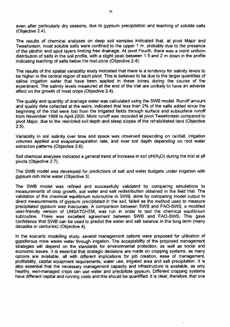
even after particularly dry seasons, due to gypsum precipitation and leaching of soluble salts(Objective 2.4).

The results of chemical analyses on deep soil samples indicated that, at pivot Major andTweefontein, most soluble salts were confined to the upper 1 m, probably due to the presenceof the plinthic and spoil layers limiting free drainage. At pivot Fourth, there was a more uniformdistribution of salts in the soil profile, with a slight peak between 1.5 and 2 m down in the profileindicating leaching of salts below the root-zone (Objective 2.4).

The results of the spatial variability study indicated that there is a tendency for salinity levels tobe higher in the central region of each pivot. This is believed to be due to the larger quantities ofsaline irrigation water that have been applied in these zones during the course of theexperiment. The salinity levels measured at the end of the trial are unlikely to have an adverseeffect on the growth of most crops (Objective 2.4).

The quality and quantity of drainage water was calculated using the SWB model. Runoff amountand quality data collected at the weirs, indicated that less than 2% of the salts added since thebeginning of the trial were lost from the irrigated fields through surface and subsurface runofffrom November 1999 to April 2000. More runoff was recorded at pivot Tweefontein compared topivot Major, due to the restricted soil depth and steep slopes of the rehabilitated land (Objective2.5).

Variability in soil salinity over time and space was observed depending on rainfall, irrigationvolumes applied and evapotranspiration rate, and over soil depth depending on root waterextraction patterns (Objective 2.6).

Soil chemical analyses indicated a general trend of increase in soil pH(H2O) during the trial at allpivots (Objective 2.7).

The SWB model was developed for predictions of salt and water budgets under irrigation withgypsum rich mine water (Objective 3).

The SWB model was refined and successfully validated by comparing simulations tomeasurements of crop growth, soil water and salt redistribution obtained in the field trial. Thevalidation of the chemical equilibrium subroutine in SWB, done by comparing model output todirect measurements of gypsum precipitated in the soil, failed as the method used to measureprecipitated gypsum was inaccurate. A comparison between SWB and FAO-SWS, a modifieduser-friendly version of UNSATCHEM, was run in order to test the chemical equilibriumsubroutine. There was excellent agreement between SWB and FAO-SWS. This gaveconfidence that SWB can be used to predict the water and salt balance in the long term (manydecades or centuries) (Objective 4).

In the scenario modelling study, several management options were proposed for utilization ofgypsiferous mine waste water through irrigation. The acceptability of the proposed managementstrategies will depend on the standards for environmental protection, as well as social andeconomic issues. It is essential that strategic decisions are made on cropping systems, as manyoptions are available, all with different implications for job creation, ease of management,profitability, capital equipment requirements, water use, irrigated area and salt precipitation. It isalso essential that the necessary management capacity and infrastructure is available, as onlyhealthy, well-managed crops can use water and precipitate gypsum. Different cropping systemshave different capital and running costs and this should be quantified. It is clear, therefore, that one

Xll

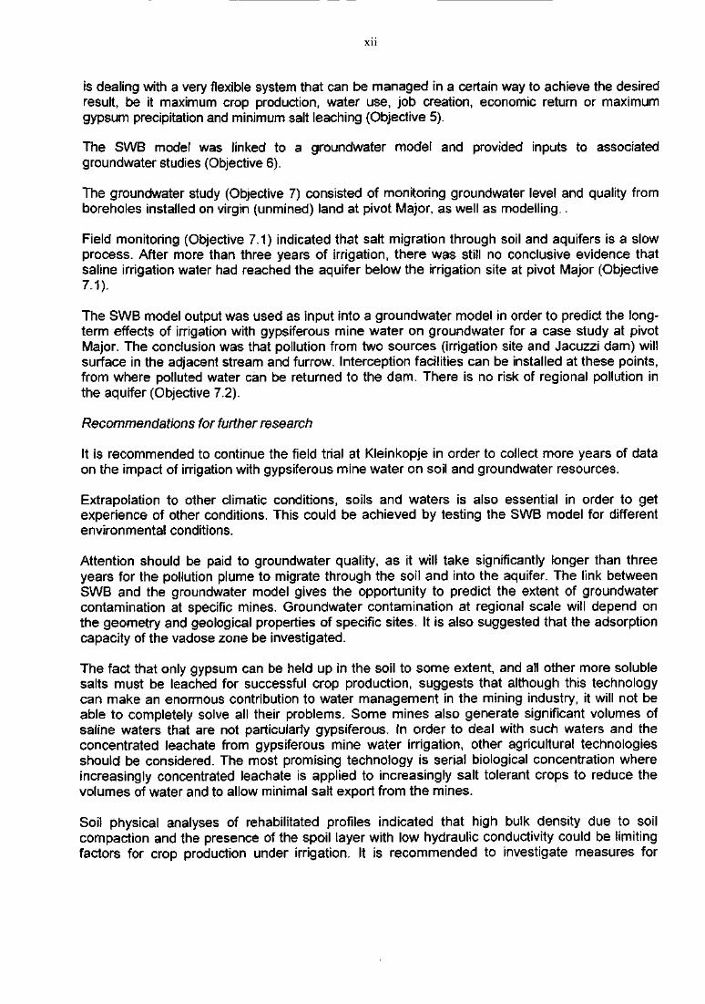
is dealing with a very flexible system that can be managed in a certain way to achieve the desiredresult, be it maximum crop production, water use, job creation, economic return or maximumgypsum precipitation and minimum salt leaching (Objective 5).

The SWB model was linked to a groundwater model and provided inputs to associatedgroundwater studies (Objective 6).

The groundwater study (Objective 7) consisted of monitoring groundwater level and quality fromboreholes installed on virgin (unmined) land at pivot Major, as well as modelling..

Field monitoring (Objective 7.1) indicated that salt migration through soil and aquifers is a slowprocess. After more than three years of irrigation, there was still no conclusive evidence thatsaline irrigation water had reached the aquifer below the irrigation site at pivot Major (Objective7.1).

The SWB model output was used as input into a groundwater model in order to predict the long-term effects of irrigation with gypsiferous mine water on groundwater for a case study at pivotMajor. The conclusion was that pollution from two sources (irrigation site and Jacuzzi dam) willsurface in the adjacent stream and furrow. Interception facilities can be installed at these points,from where polluted water can be returned to the dam. There is no risk of regional pollution inthe aquifer (Objective 7.2).

Recommendations for further research

It is recommended to continue the field trial at Kleinkopje in order to collect more years of dataon the impact of irrigation with gypsiferous mine water on soil and groundwater resources.

Extrapolation to other climatic conditions, soils and waters is also essential in order to getexperience of other conditions. This could be achieved by testing the SWB model for differentenvironmental conditions.

Attention should be paid to groundwater quality, as it will take significantly longer than threeyears for the pollution plume to migrate through the soil and into the aquifer. The link betweenSWB and the groundwater model gives the opportunity to predict the extent of groundwatercontamination at specific mines. Groundwater contamination at regional scale will depend onthe geometry and geological properties of specific sites. It is also suggested that the adsorptioncapacity of the vadose zone be investigated.

The fact that only gypsum can be held up in the soil to some extent, and all other more solublesalts must be leached for successful crop production, suggests that although this technologycan make an enormous contribution to water management in the mining industry, it will not beable to completely solve all their problems. Some mines also generate significant volumes ofsaline waters that are not particularly gypsiferous. In order to deal with such waters and theconcentrated leachate from gypsiferous mine water irrigation, other agricultural technologiesshould be considered. The most promising technology is serial biological concentration whereincreasingly concentrated leachate is applied to increasingly salt tolerant crops to reduce thevolumes of water and to allow minimal salt export from the mines.

Soil physical analyses of rehabilitated profiles indicated that high bulk density due to soilcompaction and the presence of the spoil layer with low hydraulic conductivity could be limitingfactors for crop production under irrigation. It is recommended to investigate measures for

X l l l

reducing soil compaction on rehabilitated soil profiles in order to improve land capability, ormake use of this opportunity to create a "duplex" soil from which drainage water can beretrieved for use in serial biological concentration.

There is opportunity for further improvement to SWB. The simulations with the finite-differencewater balance model were carried out without simulating salt redistribution, as theconvection/dispersion subroutine is currently being debugged. The finite-difference model hasthe potential to predict the soil water and salt balance more accurately than the cascadingmodel, once the salt redistribution subroutine becomes operational.

XIV

ACKNOWLEDGEMENTS

The research in this report emanated from a project funded by the Water Research Commissionentitled:

"The influence of Irrigation with Gypsiferous Mine Water on Soil Properties and Drainage Waterin Mpumalanga".

The Steering Committee responsible for this project, consisted of the following persons:

Mr HM du Plessis Research Manager, Water Research CommissionDr GR Backeberg Water Research CommissionMr HC van Zyl Chamber of MinesMr A McLaren Aqua PlusMr JNJ Viijoen Ingwe Coal CorporationMr ID Lamprecht Agriculture, Conservation and EnvironmentDr G Batchelor Dept. of Environmental Affairs and Tourism, PretoriaDrDJBeukes Agricultural Research Council - Institute for Soil, Climate and

Water, PretoriaMs MC Eksteen Dept. of Water Affairs and Forestry, PretoriaDr M Ligthelm Dept. of Water Affairs and Forestry, NelspruitMr KP Taylor Dept. of Agriculture, PretoriaMr N Opperman South African Agricultural Union, PretoriaProf MV Fey Dept. of Soil Science, University of Stellenbosch, formerly

Dept. of Geology, University of Cape TownMrJBConlin ESKOMMr DA du Plooy ESKOM

The contribution of the members of the Steering Committee is acknowledged gratefully.

The financing of the project by the Water Research Commission, the Technology and HumanResources for Industry Programme (THRIP, a partnership programme funded by theDepartment of Trade and Industry and managed by the National Research Foundation), andfrom the industry (Anglo Coal, Sasol, Duiker, Ingwe) is also acknowledged.

This project was only possible with the co-operation of many individuals and institutions. Theauthors therefore wish to record their sincere thanks to the following:

Mr A van der Westhuizen, who lobbied hard to ensure that generous THRIP funding wassecured and used to significantly enhance the scope of the initially planned project.

Mr HC van Zyl, who served as project leader and kept all the mining houses committed to thisproject.

Prof CF Reinhardt and Mr L Kanyomeka (Dept. Plant Production and Soil Science, University ofPretoria), as well as Mr R Meinhardt (Agricultural Research Council - Plant Protection Researchinstitute, Pesticide Dynamics Division, Roodeplaat) for carrying out the investigation on theeffect of gypsiferous mine water on herbicide activity.

XV

PHE Strohmenger (Agricultural Research Council - Institute for Soil, Climate and Water,Pretoria) for completing two laboratory trials on plant nutrition, as well as for collecting andprocessing plant nutritional data of samples collected in the field.

Mr C de Jager {Dept. Plant Production and Soil Science, University of Pretoria) for collectingand processing plant nutritional data of samples taken in the field.

Ms L Grobler (Dept. Plant Production and Soil Science, University of Pretoria) for studying theeffects of gypsum precipitation on soil properties.

Mr MP Nepfumbada (Dept. of Water Affairs and Forestry, Roodeplaat, formerly Dept. of PlantProduction and Soil Science, University of Pretoria) for his study on characterization of soilmaterial.

Prof MV Fey and Mr R Campbell (Dept. of Geology, University of Cape Town) for analysingdeep soil samples.

Mr G Ascough (School of Bioresources Engineering and Environmental Hydrology, University ofNatal) for operating the GPS unit during the study on soil salinity spatial distribution, processingthe data, and producing the salinity maps on ArcView.

Ms I van der Stoep (Dept. of Agricultural Engineering, University of Pretoria) for testing timedomain reflectometry for measurement of volumetric soil water content and soil salinity.

Mr JJB Pretorius (Dept. Plant Production and Soil Science, University of Pretoria) and Mr OTDoyer (Dept. of Agricultural Economics, University of Pretoria) for their economic analysis ofscenario simulations with the Soil Water Balance (SWB) model.

Mr G Narciso (Agricultural Research Council - Institute for Soil, Climate and Water, Pretoria) foranalysing spatial variability of crop performance and yield with remote sensing.

Mr R Grobbelaar (Institute for Groundwater Studies, University of the Free State, Bloemfontein)for collecting and processing data from the boreholes.

Mr Werner Sullwald (AMFARMS) as well as Gert and Neels Smith (Smith Bros) who whereresponsible for the farming practices during the course of the field trial.

Mr RD Garner (Anglo Coal Environmental Services, Witbank) for managing meetings andsupplying water consumption and irrigation water quality data.

Mr E Meier for his dedication to managing the field trial and supporting the farming company (asrepresentative of Kleinkopje Colliery)

Kleinkopje Colliery (Witbank) for funding, installing the irrigation system and preparing the landat the experimental site.

Finally, a special word of thanks to Mr HM du Plessis (Water Research Commission) whosevision, guidance and encouragement throughout this project have been inspirational to thewhole research team.

XVI

TABLE OF CONTENTS

List of Tables xx

List of Figures xxiv

List of Symbols xxii

1. INTRODUCTION 1

1.1. Statement of the problem 1

1.2. Background 2

1.3. Objectives of the project 3

1.4. Approach 4

2. FIELD MONITORING AND LABORATORY EXPERIMENTS 7

2.1. Introduction 7

2.2. Materials and methods - Field monitoring 7

2.2.1. Irrigation waters 92.2.2. Irrigation pivots 92.2.3. Irrigation water treatments 112.2.4. Atmospheric measurements 122.2.5. Soil measurements 122.2.6. Irrigation water chemical analyses 142.2.7. Characterization of soil material 142.2.8. Soil analyses 152.2.9. Measurement of precipitated gypsum 152.2.10. Evaluation of changes in soil salinity distribution on the irrigatedareas 162.2.11. Runoff amounts and quality 172.2.12. Installation of monitoring boreholes 17

2.2.12.1. Siting of the boreholes 172.2.12.2. Drilling 172.2.12.3. Geology and hydrogeology 192.2.12.4. Piezometer installation 192.2.12.5. Hydraulic characteristics of the aquifer 19

2.2.13. Crop measurements 21

2.3. Results of field monitoring 21

2.3.1. Characterization of soil material 212.3.1.1. Soil classification and texture 222.3.1.2. Soil bulk density and porosity 222.3.1.3. Water retention characteristics 22

XVII

2.3.1.4. Hydraulic conductivity characteristics 262.3.1.5. Solute transport characteristics 302.3.1.6. Gypsum precipitation characteristics 32

2.3.2. Crops 332.3.2.1. Yield 332.3.2.2. Plant nutrition 36

2.3.3. Soils 362.3.3.1. Chemical properties 362.3.3.2. Spatial variability of soil salinity 51

2.3.4. Waters 562.3.4.1. Irrigation water quality 562.3.4.2. Runoff 582.3.4.3. Groundwater 61

2.3.4.3.1. Groundwater quality 612.3.4.3.2. Groundwater levels 63

2.4. Glasshouse and laboratory experiments 65

2.4.1. Plant nutrition 65

2.4.2. Herbicide effects 66

3. SOIL WATER BALANCE MODEL 67

3.1. Model description 67

3.2. Model validation 703.2.1. Soil water balance and crop growth 703.2.2. Soil water redistribution 733.2.3. Salt redistribution 793.2.4. Gypsum precipitation 853.2.5. Comparison between SWB and FAO-SWS 87

4. SCENARIO SIMULATIONS 89

4.1. Introduction 894.2. Materials and methods 89

4.2.1. Long-term effects of cropping systems and environmental impact 894.2.2. Modelling the decision process with MCDM techniques 904.2.3. Economic impact 914.2.4. Analysis 91

4.3. Results and discussion 934.4. Conclusions 95

5. GROUNDWATER MODELLING 97

5.1. Model description and scenario modelling 97

5.2. Governing equations for modelling polfution transport 98

5.3. Hydraulic variables and constraints 101

XV111

5.3.1. Transmissivity and hydraulic conductivity5.3.2. Storativity and effective porosity5.3.3. Regional water table gradient, dispersion and convection5.3.4. Boundaries5.3.5. Sources of water5.3.6. Sinks

5.4. Links between the irrigation and the groundwater model

5.5. Discussion of modelling results

6. CONCLUSIONS AND RECOMMENDATIONS

7. REFERENCES

8. CAPACITY BUILDING

9. TECHNOLOGY TRANSFER

Tables

Automated tensiometers

Methods for characterization of soil material

APPENDIX A:

APPENDIX B:

APPENDIX C:

APPENDIX D:

APPENDIX E:

APPENDIX F:

APPENDIX G:

APPENDIX H:

APPENDIX I:

APPENDIX J:

APPENDIX K:

APPENDIX L:

Methods of measurement of gypsum precipitated in the soil(Soil Science Laboratory, University of Pretoria)

Calculation of the gypsum saturation index as a method fordetecting gypsum in soils, and a preliminary study ofsulphate adsorption in soils irrigated with saline mine waterat Kleinkopje Colliery (Dept. of Geology, University of CapeTown)

Borehole logs

Results from pumping test analysis

Solute transport characteristics breakthrough curves

Chemistry of soils and regolith irrigated with gypsiferousmine water

Results of chemical analyses of borehole water samples

Growth and nutrient composition of Triticum aestivum L. asaffected by nutritional management under sulphate salinity

Herbicide effects

101101101102103103

103

103

106

112

120

121

125

203

206

214

218

228

233

238

241

252

263

271

XX

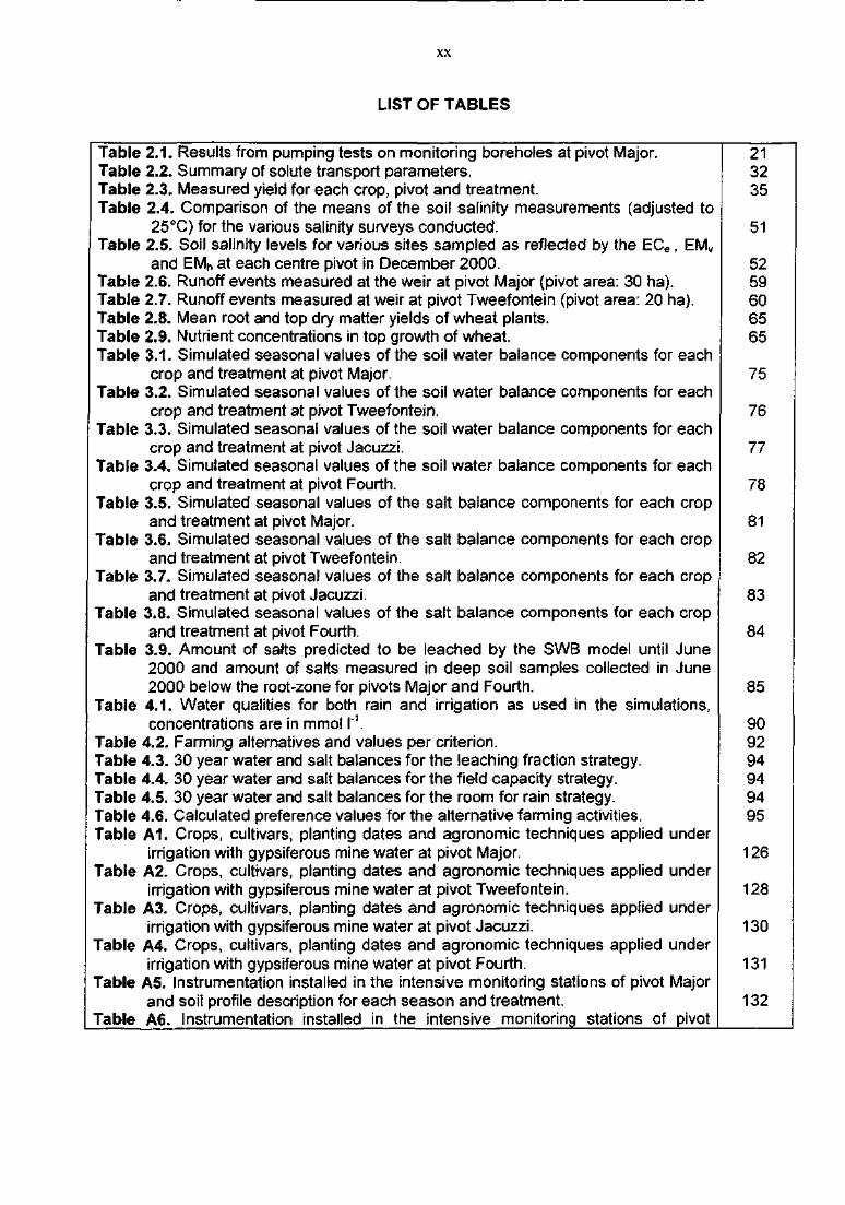
LIST OF TABLES

Table 2.1. Results from pumping tests on monitoring boreholes at pivot Major.Table 2.2. Summary of solute transport parameters.Table 2.3. Measured yield for each crop, pivot and treatment.Table 2.4. Comparison of the means of the soil salinity measurements (adjusted to

25°C) for the various salinity surveys conducted.Table 2.5. Soil salinity levels for various sites sampled as reflected by the ECe, EMV

and EMh at each centre pivot in December 2000.Table 2.6. Runoff events measured at the weir at pivot Major (pivot area: 30 ha).Table 2.7. Runoff events measured at weir at pivot Tweefontein (pivot area: 20 ha).Table 2.8. Mean root and top dry matter yields of wheat plants.Table 2.9. Nutrient concentrations in top growth of wheat.Table 3.1. Simulated seasonal values of the soil water balance components for each

crop and treatment at pivot Major.Table 3.2. Simulated seasonal values of the soil water balance components for each

crop and treatment at pivot Tweefontein.Table 3.3. Simulated seasonal values of the soil water balance components for each

crop and treatment at pivot Jacuzzi.Table 3.4. Simulated seasonal values of the soil water balance components for each

crop and treatment at pivot Fourth.Table 3.5. Simulated seasonal values of the salt balance components for each crop

and treatment at pivot Major.Table 3.6. Simulated seasonal values of the salt balance components for each crop

and treatment at pivot Tweefontein.Table 3.7. Simulated seasonal values of the salt balance components for each crop

and treatment at pivot Jacuzzi.Table 3.8. Simulated seasonal values of the salt balance components for each crop

and treatment at pivot Fourth.Table 3.9. Amount of salts predicted to be leached by the SWB model until June

2000 and amount of salts measured in deep soil samples collected in June2000 below the root-zone for pivots Major and Fourth.

Table 4.1. Water qualities for both rain and irrigation as used in the simulations,concentrations are in mmo! I'1.

Table 4.2. Farming alternatives and values per criterion.Table 4.3. 30 year water and salt balances for the leaching fraction strategy.Table 4.4. 30 year water and salt balances for the field capacity strategy.Table 4.5. 30 year water and salt balances for the room for rain strategy.Table 4.6. Calculated preference values for the alternative farming activities.Table A1. Crops, cultivars, planting dates and agronomic techniques applied under

irrigation with gypsiferous mine water at pivot Major.Table A2. Crops, cultivars, planting dates and agronomic techniques applied under

irrigation with gypsiferous mine water at pivot Tweefontein.Table A3. Crops, cultivars, planting dates and agronomic techniques applied under

irrigation with gypsiferous mine water at pivot Jacuzzi.Table A4. Crops, cuttivars, planting dates and agronomic techniques applied under

irrigation with gypsiferous mine water at pivot Fourth.Table A5. Instrumentation installed in the intensive monitoring stations of pivot Major

and soil profile description for each season and treatment.Table A6. Instrumentation installed in the intensive monitoring stations of pivot

213235

51

5259606565

75

76

77

78

81

82

83

84

85

909294949495

126

128

130

131

132

XXI

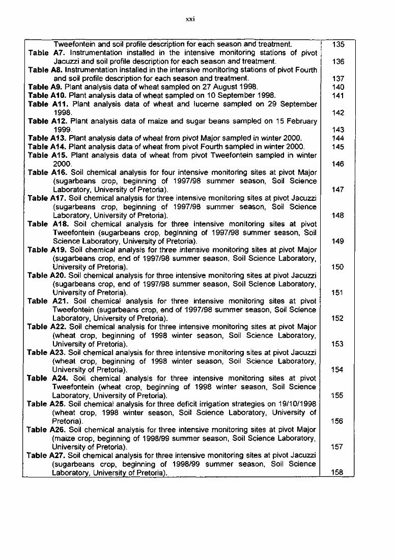
Tweefontein and soil profile description for each season and treatment.Table A7. Instrumentation installed in the intensive monitoring stations of pivot

Jacuzzi and soil profile description for each season and treatment.Table A8. Instrumentation installed in the intensive monitoring stations of pivot Fourth

and soil profile description for each season and treatment.Table A9. Plant analysis data of wheat sampled on 27 August 1998.Table A10. Plant analysis data of wheat sampled on 10 September 1998.Table A11. Plant analysis data of wheat and lucerne sampled on 29 September

1998.Table A12. Plant analysis data of maize and sugar beans sampled on 15 February

1999.Table A13. Plant analysis data of wheat from pivot Major sampled in winter 2000.Table A14. Plant analysis data of wheat from pivot Fourth sampled in winter 2000.Table A15. Plant analysis data of wheat from pivot Tweefontein sampled in winter

2000.Table A16. Soil chemical analysis for four intensive monitoring sites at pivot Major

(sugarbeans crop, beginning of 1997/98 summer season, Soil ScienceLaboratory, University of Pretoria).

Table A17. Soil chemical analysis for three intensive monitoring sites at pivot Jacuzzi(sugarbeans crop, beginning of 1997/98 summer season, Soil ScienceLaboratory, University of Pretoria).

Table A18. Soil chemical analysis for three intensive monitoring sites at pivotTweefontein (sugarbeans crop, beginning of 1997/98 summer season, SoilScience Laboratory, University of Pretoria).

Table A19. Soil chemical analysis for three intensive monitoring sites at pivot Major(sugarbeans crop, end of 1997/98 summer season, Soil Science Laboratory,University of Pretoria).

Table A20. Soil chemical analysis for three intensive monitoring sites at pivot Jacuzzi(sugarbeans crop, end of 1997/98 summer season, Soil Science Laboratory,University of Pretoria).

Table A21. Soil chemical analysis for three intensive monitoring sites at pivotTweefontein (sugarbeans crop, end of 1997/98 summer season, Soil ScienceLaboratory, University of Pretoria).

Table A22. Soil chemical analysis for three intensive monitoring sites at pivot Major(wheat crop, beginning of 1998 winter season, Soil Science Laboratory,University of Pretoria).

Table A23. Soil chemical analysis for three intensive monitoring sites at pivot Jacuzzi(wheat crop, beginning of 1998 winter season, Soil Science Laboratory,University of Pretoria).

Table A24. Soil chemical analysis for three intensive monitoring sites at pivotTweefontein (wheat crop, beginning of 1998 winter season, Soil ScienceLaboratory, University of Pretoria).

Table A25. Soil chemical analysis for three deficit irrigation strategies on 19/10/1998(wheat crop, 1998 winter season, Soil Science Laboratory, University ofPretoria).

Table A26. Soil chemical analysis for three intensive monitoring sites at pivot Major(maize crop, beginning of 1998/99 summer season, Soil Science Laboratory,University of Pretoria).

Table A27. Soil chemical analysis for three intensive monitoring sites at pivot Jacuzzi(sugarbeans crop, beginning of 1998/99 summer season, Soil ScienceLaboratory, University of Pretoria).

135

136

137140141

142

143144145

146

147

148

149

150

151

152

153

154

155

156

157

158

XXI1

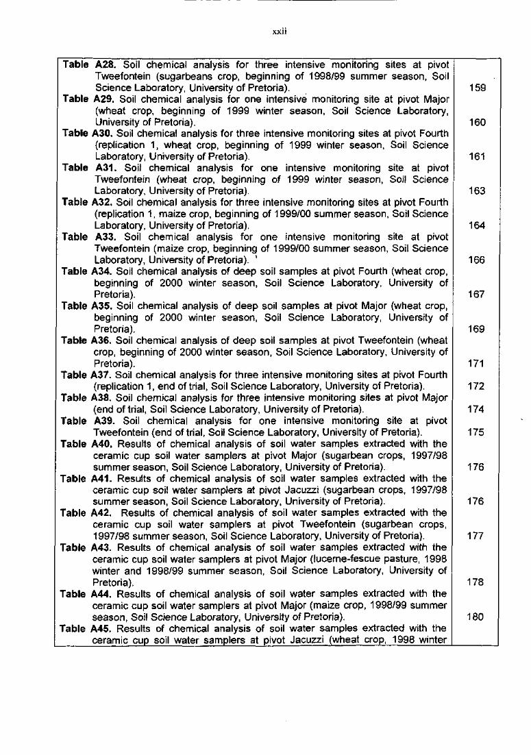
Table A28. Soil chemical analysis for three intensive monitoring sites at pivotTweefontein (sugarbeans crop, beginning of 1998/99 summer season, SoilScience Laboratory, University of Pretoria).

Table A29. Soil chemical analysis for one intensive monitoring site at pivot Major(wheat crop, beginning of 1999 winter season, Soil Science Laboratory,University of Pretoria).

Table A30. Soil chemical analysis for three intensive monitoring sites at pivot Fourth(replication 1, wheat crop, beginning of 1999 winter season, Soil ScienceLaboratory, University of Pretoria).

Table A31. Soil chemical analysis for one intensive monitoring site at pivotTweefontein (wheat crop, beginning of 1999 winter season, Soil ScienceLaboratory, University of Pretoria).

Table A32. Soil chemical analysis for three intensive monitoring sites at pivot Fourth(replication 1, maize crop, beginning of 1999/00 summer season, Soil ScienceLaboratory, University of Pretoria).

Table A33. Soil chemical analysis for one intensive monitoring site at pivotTweefontein (maize crop, beginning of 1999/00 summer season, Soil ScienceLaboratory, University of Pretoria). *

Table A34. Soil chemical analysis of deep soil samples at pivot Fourth (wheat crop,beginning of 2000 winter season, Soil Science Laboratory, University ofPretoria).

Table A35. Soil chemical analysis of deep soil samples at pivot Major (wheat crop,beginning of 2000 winter season, Soil Science Laboratory, University ofPretoria).

Table A36. Soil chemical analysis of deep soil samples at pivot Tweefontein (wheatcrop, beginning of 2000 winter season, Soil Science Laboratory, University ofPretoria).

Table A37. Soil chemical analysis for three intensive monitoring sites at pivot Fourth(replication 1, end of trial, Soil Science Laboratory, University of Pretoria).

Table A38. Soil chemical analysis for three intensive monitoring sites at pivot Major(end of trial, Soil Science Laboratory, University of Pretoria).

Table A39. Soil chemical analysis for one intensive monitoring site at pivotTweefontein (end of trial, Soil Science Laboratory, University of Pretoria).

Table A40. Results of chemical analysis of soil water samples extracted with theceramic cup soil water samplers at pivot Major (sugarbean crops, 1997/98summer season, Soil Science Laboratory, University of Pretoria).

Table A41. Results of chemical analysis of soil water samples extracted with theceramic cup soil water samplers at pivot Jacuzzi (sugarbsan crops, 1997/98summer season, Soil Science Laboratory, University of Pretoria).

Table A42. Results of chemical analysis of soil water samples extracted with theceramic cup soil water samplers at pivot Tweefontein (sugarbean crops,1997/98 summer season, Soil Science Laboratory, University of Pretoria).

Table A43. Results of chemical analysis of soil water samples extracted with theceramic cup soil water samplers at pivot Major (lucerne-fescue pasture, 1998winter and 1998/99 summer season, Soil Science Laboratory, University ofPretoria).

Table A44. Results of chemical analysis of soil water samples extracted with theceramic cup soil water samplers at pivot Major (maize crop, 1998/99 summerseason, Soil Science Laboratory, University of Pretoria).

Table A45. Results of chemical analysis of soil water samples extracted with theceramic cup soil water samplers at pivot Jacuzzi (wheat crop, 1998 winter

159

160

161

163

164

166

167

169

171

172

174

175

176

176

177

178

180

xxni

season, Soil Science Laboratory, University of Pretoria).Table A46. Results of chemical analysts of soil water samples extracted with the

ceramic cup soil water samplers at pivot Tweefontein (wheat crop, 1998 winterseason, Soil Science Laboratory, University of Pretoria).

Table A47. Results of chemical analysis of soil water samples extracted with theceramic cup soil water samplers at pivot Fourth (wheat crop, 1999 winterseason, Soil Science Laboratory, University of Pretoria).

Table A48. Results of chemical analysis of soil water samples extracted with theceramic cup soil water samplers at pivot Fourth (maize crop, 1999/00 summerseason, Soil Science Laboratory, University of Pretoria).

Table A49. Results of chemical analysis of soil water samples extracted with theceramic cup soil water samplers at pivot Fourth (wheat crop, 2000 winterseason, Soil Science Laboratory, University of Pretoria).

Table A50. Results of chemical analysis for Jacuzzi water (Kleinkopje Colliery,personal communication).

Table A51. Results of chemical analysis for Tweefontein dam water (KleinkopjeColliery, personal communication).

Table A52. Results of chemical analysis for Jacuzzi water (Soil Science Laboratory,University of Pretoria).

Table A53. Results of chemical analysis for Tweefontein dam water (Soil ScienceLaboratory, University of Pretoria).

Table A54. Results from chemical analyses of water samples from the Jacuzzi dam.Table A55. Summary of soil characterization tests performed.Table A56. Summary of soil characteristics data.Table A57. Van Genuchten soil hydraulic characteristic parameters.Table A58. Brooks-Corey soil hydraulic characteristic parameters.Table A59. Campbell soil hydraulic characteristic parameters.Table E1. Composition and gypsum saturation indices of a saturated gypsum

solution.Table E2. Composition and gypsum saturation indices of solutions equilibrated with

soils and treated with gypsum as indicated.Table K1. Mean root and top dry matter yields of wheat plants.Table K2. Nutrient concentrations in top growth of wheat.Table L1. Chemical composition of mine water used in the herbicide tank mixture.Table L2. Quantitative results of the mine water herbicide tank-mix.Table L3. Effect of gypsum in soil on the biological activity of atrazine across ten

herbicide concentrations.Table L4. Effect of gypsum in soil on the biologica! activity of metolachlor across ten

herbicide concentrations.

181

182

183

184

185

188

192

195

195196197198199201202

219

220267268273274

275

275

XXIV

LIST OF FIGURES

Figure 2.1. Locality plan of Kleinkopje Colliery.Figure 2.2. Mine map with the location of the pivots, dams, plants, infrastructure and

mining areas.Figure 2.3. Typical layout of irrigation pivot.Figure 2.4. Locality plan of the irrigation pivot Major showing the positions of

boreholes.Figure 2.5. Typical geological log in the irrigation pivot Major area.Figure 2.6. Typical installation of a piezometer in borehole at the irrigation pivot Major.Figure 2.7. Water retention characteristics for pivot Major on the surface. The

Campbell functions (solid lines) are fitted to the sets of data for Major 1 (upperbound) and for Major 3 (lower bound).

Figure 2.8. Water retention characteristics for pivot Major at 0.5 m below the surface.The Campbell functions (solid lines) are fitted to the sets of data for Major 1(upper bound) and for Major 4 (lower bound).

Figure 2.9. Water retention characteristic for pivot Major on the plinthite layer, 1.0 mbelow the surface. The Campbell function (solid line) is fitted to the data set.

Figure 2.10. Water retention characteristics for topsoil and spoil material at pivotTweefontein. The Campbell functions (solid lines) are fitted to the data sets.

Figure 2.11. Hydraulic conductivity characteristic for topsoils and spoil material atpivot Jacuzzi. The mathematical functions for surface and spoil layer (solidlines) were derived by simultaneously optimizing the van Genuchtencharacteristic functions to the water retention and hydraulic conductivity data.

Figure 2.12. Hydraulic conductivity characteristic for topsoil and spoil material at pivotTweefontein. The mathematical functions for surface and spoil layer (solidlines) were derived by simultaneously optimizing the van Genuchtencharacteristic functions to the water retention and hydraulic conductivity data.

Figure 2.13. Hydraulic conductivity characteristic for topsoils and plinthite material atpivot Major. The mathematical functions for surface and plinthite layer (solidlines) were derived by simultaneously optimizing the van Genuchtencharacteristic functions to the water retention and hydraulic conductivity data.

Figure 2.14. Spatial distribution of hydraulic conductivities at 60 mm tension at pivotMajor.

Figure 2.15. Spatial distribution of hydraulic conductivities at 210 mm tension at pivotMajor.

Figure 2.16. Breakthrough characteristic for distilled water injection of sample frompivot Fourth. .

Figure 2.17. Breakthrough characteristic for CaSO4 and KCI solution injection ofsample from pivot Fourth.

Figure 2.18. Water retention characteristics of samples from gypsum precipitationcolumns of 8 and 30 Mg ha"1. The field cores (dashed lines) represent theupper and lower bound water retention functions (Figure 2.8).

Figure 2.19. Soil pH(H2O) at pivot Major (field capacity treatment) taken at seasonalintervals as a function of depth (cm).

Figure 2.20. Soil pH(H2O) at pivot Tweefontein (field capacity treatment) taken atseasonal intervals as a function of depth (cm).

Figure 2.21. Soil pH(H2O) at pivot Fourth (field capacity treatment) taken at seasonalintervals as a function of depth (cm).

Figure 2.22. Soil pH(H2O) at pivot Jacuzzi (field capacity treatment) taken at seasonal

8

1011

182020

24

24

25

25

27

27

28

29

29

31

31

33

38

38

38

XXV

intervals as a function of depth (cm). 38Figure 2.23. Electrical conductivity (mS m~1) of the saturated soil extract at pivot Major

(leaching fraction treatment) taken at seasonal intervals as a function of depth(cm). 39

Figure 2.24. Electrical conductivity (mS m'1) of the saturated soil extract at pivot Major(field capacity treatment) taken at seasonal intervals as a function of depth(cm). 39

Figure 2.25. Electrical conductivity (mS m'1) of the saturated soil extract at pivot Major(deficit treatment) taken at seasonal intervals as a function of depth (cm). 39

Figure 2.26. Soluble calcium content (cmolc kg"1) of the saturated soil extract at pivotMajor (leaching fraction treatment) taken at seasonal intervals as a function ofdepth (cm). 40

Figure 2.27. Soluble calcium content (cmolc kg"1) of the saturated soil extract at pivotMajor (field capacity treatment) taken at seasonal intervals as a function ofdepth (cm). 40

Figure 2.28. Soluble calcium content (cmolc kg"1) of the saturated soil extract at pivotMajor (deficit treatment) taken at seasonal intervals as a function of depth(cm). 40

Figure 2.29. Soluble magnesium content (cmolc kg"1) of the saturated soil extract atpivot Major (leaching fraction treatment) taken at seasonal intervals as afunction of depth (cm). 41

Figure 2.30. Soluble magnesium content (cmolc kg"1) of the saturated soil extract atpivot Major (field capacity treatment) taken at seasonal intervals as a functionof depth (cm). 41

Figure 2.31. Soluble magnesium content (cmolc kg"1) of the saturated soil extract atpivot Major (deficit treatment) taken at seasonal intervals as a function of depth(cm). 41

Figure 2.32. Soluble potassium content (cmolc kg"1) of the saturated soil extract atpivot Major (leaching fraction treatment) taken at seasonal intervals as afunction of depth (cm). 42

Figure 2.33. Soluble potassium content (cmolc kg"1) of the saturated soil extract atpivot Major (field capacity treatment) taken at seasonal intervals as a functionof depth (cm). 42

Figure 2.34. Soluble potassium content (cmolc kg'1) of the saturated soil extract atpivot Major (deficit treatment) taken at seasonal intervals as a function of depth(cm). 42

Figure 2.35. Sulphate content (cmolc kg"1) of the saturated soil extract at pivot Major(leaching fraction treatment) taken at seasonal intervals as a function of depth(cm). 43

Figure 2.36. Sulphate content (cmolc kg'1) of the saturated soil extract at pivot Major(field capacity treatment) taken at seasonal intervals as a function of depth(cm). 43

Figure 2.37. Sulphate content (cmolc kg"1) of the saturated soit extract at pivot Major(deficit treatment) taken at seasonal intervals as a function of depth (cm). 43

Figure 2.38. Exchangeable calcium content (cmo!c kg'1) of the saturated soil extract atpivot Major (leaching fraction treatment) taken at seasonal intervals as afunction of depth (cm). 44

Figure 2.39. Exchangeable calcium content (cmolc kg'1) of the saturated soil extract atpivot Major (field capacity treatment) taken at seasonal intervals as a functionof depth (cm). 44

Figure 2.40. Exchangeable calcium content (cmolc kg1) of the saturated soil extract at

XXV!

pivot Major (deficit treatment) taken at seasonal intervals as a function of depth(cm).

Figure 2.41. Exchangeable potassium content (cmolc kg"1) of the saturated soil extractat pivot Major (leaching fraction treatment) taken at seasonal intervals as afunction of depth (cm).

Figure 2.42. Exchangeable potassium content (cmolc kg"1) of the saturated soil extractat pivot Major (field capacity treatment) taken at seasonal intervals as afunction of depth (cm).

Figure 2.43. Exchangeable potassium content (cmolc kg"1) of the saturated soil extractat pivot Major (deficit treatment) taken at seasonal intervals as a function ofdepth (cm).

Figure 2.44. Calculated CEC (cmolc kg'1) at pivot Major (leaching fraction treatment)taken at seasonal intervals as a function of depth (cm).

Figure 2.45. Calculated CEC (cmolc kg"1) at pivot Major (field capacity treatment)taken at seasonal intervals as a function of depth (cm).

Figure 2.46. Calculated CEC (cmolc kg"1) at pivot Major (deficit treatment) taken atseasonal intervals as a function of depth (cm).

Figure 2.47. Soil pH(H2O) at pivot Major as a function of depth (m) in June 2000.Figure 2.48. Soil pH(H2O) at pivot Fourth as a function of depth (m) in June 2000.Figure 2.49. Soil pH(H2O) at pivot Tweefontein as a function of depth (m) in June

2000.Figure 2.50. Electrical conductivity (mS m"1) of the saturated soil extract at pivot Major

as a function of depth (m) in June 2000.Figure 2.51. Electrical conductivity (mS m'1) of the saturated soil extract at pivot

Fourth as a function of depth (m) in June 2000.Figure 2.52. Electrical conductivity (mS m'1) of the saturated soil extract at pivot

Tweefontein as a function of depth (m) in June 2000.Figure 2.53. Soluble calcium content (cmolc kg*1) of the saturated soil extract at pivot

Major as a function of depth (m) in June 2000.Figure 2.54. Soluble calcium content (cmolc kg'1) of the saturated soil extract at pivot

Fourth as a function of depth (m) in June 2000.Figure 2.55. Soluble calcium content (cmolc kg"1) of the saturated soil extract at pivot

Tweefontein as a function of depth (m) in June 2000.Figure 2.56. Sulphate content (cmolc kg"1) of the saturated soil extract at pivot Major

as a function of depth (m) in June 2000.Figure 2.57. Sulphate content (cmolc kg'1) of the saturated soil extract at pivot Fourth

as a function of depth (m) in June 2000.Figure 2.58. Sulphate content (cmolc kg"1) of the saturated soil extract at pivot

Tweefontein as a function of depth (m) in June 2000.Figure 2.59. Spatial distribution of salinity in the upper soil profile (ECe over 0-60 cm)

of the Tweefontein centre pivot showing changes over the study period. The 1m contour lines illustrate a downward slope from West to East.

Figure 2.60. Spatial distribution of salinity in the upper soil profile (ECe over 0-60 cm)of the Major centre pivot showing changes over the study period. The 1 mcontour lines illustrate a downward slope from North to South.

Figure 2.61. Spatial distribution of salinity in the upper soil profile (ECe over 0-60 cm)of the Fourth centre pivot showing changes over the study period. Individualfigures on the transect for 1999 are in mS m'1. The 1 m contour lines illustratea downward slope from North-West to South-East.

Figure 2.62. Approximate stage curve for the mine water holding dam.Figure 2.63. Results from chemical analyses on water samples from monitoring

44

45

45

45

46

46

464747

47

48

48

48

49

49

49

50

50

50

54

55

5657

XXV11

boreholes at pivot Major for NO3' and electrical conductivity.Figure 2.64. Results from chemical analyses on water samples from monitoring

boreholes at pivot Major for Na+, Mg3+ and Ca2+.Figure 2.65. Results from chemical analyses on water samples from monitoring

boreholes at pivot Major for pH, total alkalinity and SO42'.

Figure 2.66. Water levels in monitoring boreholes at the irrigation site.Figure 3.1. Soil water balance summary graph (wheat crop, winter 1999 season, pivot

Fourth, leaching fraction treatment, replication 2).Figure 3.2. Simulated (solid line) and measured (symbols) root depth (RD), leaf area

index (LAI), top and harvestable dry matter (TDM & HDM), as well as soil waterdeficit to field capacity (wheat crop, winter 1999 season, pivot Fourth, leachingfraction treatment, replication 2).

Figure 3.3. Measured and simulated soil matric potential with the cascading and finite-difference water balance model at 16 cm soil depth, as well as irrigation andrainfall (wheat crop, winter 1999 season, pivot Fourth, leaching fractiontreatment, replication 2).

Figure 3.4. Measured and simulated electrical conductivity of the soil solution for threeirrigation treatments (wheat crop, winter 1999 season, pivot Fourth, replication2).

Figure 3.5. Measured and simulated values of gypsum precipitated in the soil profilein June 2000 at pivot Major.

Figure 3.6. Amounts of gypsum precipitated in the soil profile simulated with SWB andFAO-SWS for an imaginary pasture crop after one year of irrigation withTweefontein water.

Figure 5.1. Groundwater level distribution, also showing the irrigation pivot Major anddam.

Figure 5.2. Predicted concentrations at which specific constituents will leach into thegroundwater underneath the irrigation site.

Figure 5.3. Pollution plumes for hydraulic gradients 1:10, 1:100 and 1:1000 from northto south through a pollution source over a period of 3 years. The scale for eachdiagram is 1000 m from left to right.

Figure 5.4. Stream intersecting a pollution plume (left). Stream and borehole whichabstract water, intersect the same pollution plume.

Figure 5.5. Development of the pollution plume with no retardation, on the assumptionthat pollution has moved vertically into the aquifer over the whole irrigationpivot.

Figure 5.6. Breakthrough curves for positions indicated in Figure 5.5 (fourth diagram).Figure 5.7. Potential development of the pollution plumes from the irrigation area and

mine water dam.Figure B1. Schematic view of automated tensiometer and logging system for

recording soil matric pressure head. (Three or four tensiometers were installedat each intensive monitoring site).

Figure C1. Schematic layout of the controlled outflow cell apparatus for determinationof the water retention characteristic of undisturbed and packed samples.

Figure C2. Constant head permeameter for measuring saturated hydraulicconductivity.

Figure C3. Schematic of the Bruce-Klute diffusivity cell assembly.Figure C4. Schematic views of the tension (left) and double ring (right) infiltrometers.Figure C5. Schematic view of the equilibrated soluble mass column leach test

apparatus.Figure E1. Sulphate concentration in solution before and after equilibration with four

62

62

6364

71

72

74

80

86

88

98

100

102

102

104104

105

205

208

209210212

213

XXVI11

soils. PM2 = Pivot Major (field capacity treatment); PM4 = Pivot Major (outsidepivot).

Figure E2. Adsorption of sulphate by soils from sodium sulphate solutions. Best-fitLangmuir and Freundlich isotherms are indicated. PM4 = Pivot Major (outsidepivot); PF4 = Pivot Fourth (outside pivot).

Figure E3. Sulphate adsorption by soils from gypsum solutions. A best-fit Freundlichisotherm is indicated. PM4 = Pivot Major (outside pivot); PF4 = Pivot Fourth(outside pivot).

Figure E4. Calcium adsorption by soils from gypsum solutions. A best-fit Freundlichisotherm for two of the soils is indicated. PM4 = Pivot Major (outside pivot);PF4 = Pivot Fourth (outside pivot).

Figure E5. Plot of sulphate adsorbed vs. calcium adsorbed by three soils fromgypsum solutions. PM4 = Pivot Major (outside pivot); PF4 = Pivot Fourth(outside pivot).

Figure F1. Geological log of borehole BH1 at pivot Major.Figure F2. Geological log of borehole BH4 at pivot Major.Figure F3. Geological log of borehole BH5 at pivot Major.Figure F4. Geological log of borehole BH6 at pivot Major.Figure F5. Geological log of borehole BH7 at pivot Major.Figure F6. Geological log of borehole BH8 at pivot Major.Figure F7. Geological log of borehole BH9 at pivot Major.Figure G1. Pumping test curve for groundwater monitoring borehole BH3 at pivot

Major.Figure G2. Pumping test curve for groundwater monitoring borehole BH4 at pivot

Major.Figure G3. Pumping test curve for groundwater monitoring borehole BH5 at pivot

Major.Figure G4. Pumping test curve for groundwater monitoring borehole BH6 at pivot

Major.Figure G5. Pumping test curve for groundwater monitoring borehole BH7 at pivot

Major.Figure G6. Pumping test curve for groundwater monitoring borehole BH8 at pivot

Major.Figure G7. Pumping test curve for groundwater monitoring borehole BH9 at pivot

Major.Figure H1. Breakthrough characteristic for distilled water injection of sample from

pivot Tweefontein.Figure H2. Breakthrough characteristic for CaSO4 and KCI solution injection of sample

from pivot Tweefontein.Figure H3. Breakthrough characteristic for CaSO4 and KCI solution injection of sample

from pivot Major.Figure H4. Breakthrough characteristic for distilled water injection of sample from

pivot Major.Figure 11. Soluble calcium concentration (meq I"1) of the saturated paste extract (SPE)

in the field capacity treatment of pivot Major (PM2) and outside the pivot area(PM4) as a function of depth (mm).

Figure 12. Soluble calcium concentration (meq I'1) of the saturated paste extract (SPE)in the field capacity treatment of pivot Fourth (PF2) and outside the pivot area(PF4) as a function of depth (mm).

Figure 13. Soluble calcium concentration (meq I"1) of the saturated paste extract (SPE)in the field capacity treatment of pivot Tweefontein (PT2) and outside the pivot

225

225

226

226

227229230230231231232232

234

234

235

235

236

236

237

239

239

240

240

244

244

XXIX

area (PT4) as a function of depth (mm). | 245Figure 14. Soluble magnesium concentration (meq I"1) of the saturated paste extract

(SPE) in the field capacity treatment of pivot Major (PM2) and outside the pivotarea (PM4) as a function of depth (mm). 246

Figure 15. Soluble magnesium concentration (meq I"1) of the saturated paste extract(SPE) in the field capacity treatment of pivot Fourth (PF2) and outside the pivotarea (PF4) as a function of depth (mm). 246

Figure 16. Soluble magnesium concentration (meq I"1) of the saturated paste extract(SPE) in the field capacity treatment of pivot Tweefontein (PT2) and outsidethe pivot area (PT4) as a function of depth (mm). 247

Figure 17. Soluble sulphate concentration (meq I"1) of the saturated paste extract(SPE) in the field capacity treatment of pivot Major (PM2) and outside the pivotarea (PM4) as a function of depth (mm). 248

Figure 18. Soluble sulphate concentration (meq I"1) of the saturated paste extract(SPE) in the field capacity treatment of pivot Fourth (PF2) and outside the pivotarea (PF4) as a function of depth (mm). 248

Figure 19. Soluble sulphate concentration (meq I"1) of the saturated paste extract(SPE) in the field capacity treatment of pivot Tweefontein (PT2) and outsidethe pivot area (PT4) as a function of depth (mm). 249

Figure 110. NH4 acetate extractable calcium (meq kg'1) in the field capacity treatmentof pivot Major (PM2) and outside the pivot area (PM4) as a function of depth(mm). 250

Figure 111. NH4 acetate extractable calcium (meq kg'1) in the field capacity treatmentof pivot Tweefontein (PT2) and outside the pivot area (PT4) as a function ofdepth (mm). 250

Figure 112. NH4 acetate extractable magnesium (meq kg"1) in the field capacitytreatment of pivot Major (PM2) and outside the pivot area (PM4) as a functionof depth (mm). 251

Figure 113. NH4 acetate extractable magnesium (meq kg"1) in the field capacitytreatment of pivot Tweefontein (PT2) and outside the pivot area (PT4) as afunction of depth (mm). 251

Figure J1. Concentrations of aluminum, barium and boron in boreholes BH2 to BH9 atpivot Major and Jacuzzi dam. 253

Figure J2. Concentrations of bromide, calcium and chloride in boreholes BH2 to BH9at pivot Major and Jacuzzi dam. 254

Figure J3. Concentrations of chromium, copper and iron in boreholes BH2 to BH9 atpivot Major and Jacuzzi dam. 255

Figure J4. Electrical conductivity and concentrations of fluoride and lithium inboreholes BH2 to BH9 at pivot Major and Jacuzzi dam. 256

Figure J5. Concentrations of magnesium, manganese and molybdenum in boreholesBH2 to BH9 at pivot Major and Jacuzzi dam. 257

Figure J6. Concentrations of nickel and nitrogen (NO3 and NO2) in boreholes BH2 toBH9 at pivot Major and Jacuzzi dam. 258

Figure J7. pH and concentrations of phosphate and potassium in boreholes BH2 toBH9 at pivot Major and Jacuzzi dam. 259

Figure J8. Concentrations of selenium, sodium and strontium in boreholes BH2 toBH9 at pivot Major and Jacuzzi dam. 260

Figure J9. Concentrations of sulphate, total alkalinity and concentrations of vanadiumin boreholes BH2 to BH9 at pivot Major and Jacuzzi dam. 261

Figure J10. Concentrations of zinc and sodium adsorption ratio diagram for boreholesBH2 to BH9 at pivot Major and Jacuzzi dam. I 262

XXX

Figure K1. Nutrient vector analysis, interpretation of directional changes in relative drymass and nutrient status of plants differing in productivity (modified fromTimmer and Teng, 1999).

Figure K2. Relative response in nutrient concentration, content and dry mass of thesulphate salinized control treatment.

Figure M1. Nodal set-up showing upper and lower halves of layers, layer thicknesses(Az), control volumes and fluxes of vapour, (Jv) and liquid, (J,) between controlvolumes.

Figure N1. Soil water balance summary graph (wheat crop, winter 1999 season, pivotFourth, field capacity treatment, replication 2).

Figure N2. Soil water balance summary graph (wheat crop, winter 1999 season, pivotFourth, deficit irrigation treatment, replication 2).

Figure N3. Simulated (solid line) and measured (symbols) root depth (RD), leaf areaindex (LAI), top and harvestable dry matter (TDM & HDM), as well as soil waterdeficit to field capacity (wheat crop, winter 1999 season, pivot Fourth, fieldcapacity treatment, replication 2).

Figure N4. Simulated (solid line) and measured (symbols) root depth (RD), ieaf areaindex (LAI), top and harvestable dry matter (TDM & HDM), as well as soil waterdeficit to field capacity (wheat crop, winter 1999 season, pivot Fourth, deficitirrigation treatment, replication 2).

Figure N5. Measured and simulated soil matric potential with the cascading waterbalance model at different depths in the soil profile, as well as irrigation andrainfall (wheat crop, winter 1999 season, pivot Fourth, leaching fractiontreatment, replication 2).

Figure N6. Measured and simulated soil matric potential with the cascading waterbalance model at different depths in the soil profile, as well as irrigation andrainfall (wheat crop, winter 1999 season, pivot Fourth, field capacity treatment,replication 2).

Figure N7. Measured and simulated soil matric potential with the cascading waterbalance model at different depths in the soil profile, as well as irrigation andrainfall (wheat crop, winter 1999 season, pivot Fourth, deficit irrigationtreatment, replication 2).

Figure N8. Measured and simulated soil matric potential with the finite-differencewater balance model at different depths in the soil profile, as well as irrigationand rainfall (wheat crop, winter 1999 season, pivot Fourth, leaching fractiontreatment, replication 2).

Figure N9. Measured and simulated soil matric potential with the finite-differencewater balance model at different depths in the soil profile, as we!) as irrigationand rainfall (wheat crop, winter 1999 season, pivot Fourth, field capacitytreatment, replication 2).

Figure N10. Measured and simulated soil matric potential with the finite-differencewater balance model at different depths in the soil profile, as well as irrigationand rainfall (wheat crop, winter 1999 season, pivot Fourth, deficit irrigationtreatment, replication 2).

Figure N11- Measured (symbols) and simulated (line) concentration of calcium in thesoil solution (wheat crop, winter 1999 season, pivot Fourth, leaching fractiontreatment, replication 2) at different depths in the soil profile (top graph: 0.4 m;middle graph: 1.0 m; bottom graph: 1.4 m).

Figure N12. Measured (symbols) and simulated (line) concentration of magnesium inthe soil solution (wheat crop, winter 1999 season, pivot Fourth, leachingfraction treatment, replication 2) at different depths in the soil profile (top graph:

266

269

279

290

291

292

293

294

295

296

297

298

299

300

XXXI

0.4 m; middle graph: 1.0 m; bottom graph: 1.4 m). | 301Figure N13. Measured (symbols) and simulated (line) concentration of sulphate in the

soil solution (wheat crop, winter 1999 season, pivot Fourth, leaching fractiontreatment, replication 2) at different depths in the soil profile (top graph: 0.4 m;middle graph: 1.0 m; bottom graph: 1.4 m). | 302

XXX11

LIST OF SYMBOLS AND ACRONYMS

a - Intercept of Campbell 's log-log soil water retention function

ADG - Average daily gain

ADM - Adapted dilution method

AMD - Acid mine drainage

AVR - Average value ranking

A(l) - Term of the coefficient matrix

b - Slope of Campbell 's log-log water retention function

BTC - Breakthrough curve

B(l) - Term of the coefficient matrix

C - Solute concentration in the soil solution (mol I"1)

CAM - Conflict analysis method

CDE - Convection-dispersion equation

Cavg - Time weighted average concentration of a particular solute (mol I"1)

CEC - Cation exchange capacity (cmolc kg'1)

CR - Total capital requirement per m3 water used for the specific farming alternative

cv - Vapour concentration in the soil atmosphere (kg m"3)

Cy - Saturation vapour concentration (kg m"3)

CV - Control volume (m m'1)

C(0) - Concentration of the aerial node (of infiltrating water) (mol I"1)

C(l) - Term of the coefficient matrix

D - Combined diffusion and dispersion coefficient (m2 s"1); Drainage (mm); Willmott's

(1982) index of agreement

DAP - Days after sowing

DE - Deficit irrigation strategy

DM| - Dry matter increment (kg m~2)

XXX111

Do - Ionic or molecular diffusion coefficient in free water

Dv - Vapour diffusivity in soil (m2s'1)

Dv0 - Vapour diffusivity in air (m2 s"1)

D x . Dispersion coefficient in the x-direction (m d"1)

DUL - Drainage upper limit (m m"1)

D(l) - Term of the coefficient matrix containing the previous time step soluteconcentrations

E - Evaporation (m)

EA - Net present value for the specific farming alternative over 30 years

EC - Electrical conductivity (mS m"1)

ECe - Saturated soil electrical conductivity (mS m"1)

EDX - Energy dispersive X-ray

EM - Electromagnetic induction

EMh - Horizontal electromagnetic induction

EMV - Vertical electromagnetic induction

EMmean- Mean electromagnetic induction (mS m"1)

Ep - Potential evaporation (kg m"2 s"1)

ET - Evapotranspiration (m)

ej(a,b) - Difference in impact score on criterion j for those criteria for which alternative a isbetter than alternative b

FAO - Food and Agricultural Organization of the United Nations

FC - Field capacity

g - Gravitational acceleration (9.8 m s"2)

gj - Relative importance of criterion j

h - Water level above the weir (m); Hydraulic head (m); Matric pressure head (mm)

ha - Atmospheric humidity

XXXIV

hd - Air entry pressure (mm)

HDM - Harvestable dry matter (kg m"2)

HDS - Heat dissipation sensors

he - Campbell air entry parameter (mm)

hi - Inflection point where Campbell's water retention equation changes fromexponential to quadratic

hr - Fractional relative humidity

hs - Humidity of the surface

i - Time step in the finite-difference model

I - Irrigation (m)

IC - Ion chromatography

Ji - Liquid flux (kg m"2 s"1)

Ji° - Liquid flux at the surface (kg m"2 s"1)

jsd - Diffusive and dispersive solute fluxes

jsmi - Mass solute flux

Jv - Vapour flux (kg m"2 s"1)

k - Hydraulic conductivity (m d"1); Ranking for economic criterion

K - Hydraulic conductivity (kg s m~3)

Ks - Saturated hydraulic conductivity (mm h"1 or kg s m"3)

kv' - Transfer coefficient

i - Lower half of a soil layer

LAI - Leaf area index

LF - Leaching fraction

m - Pore connectivity parameter

MAE - Mean absolute error

MBE - Mass balance error

MCDM - Multiple criteria decision-making

XXXV

Mw - Molecular mass of water (kg mol'1)

n - Effective porosity; Number of criteria; Coefficient of the hydraulic conductivityfunction; Empirical constant in the solute dispersion/diffusion equation

N - Number of observations

NWM - Neutron water meter

PCM - Precipitation of salts over 30 years (Mg ha"1)

PET - Potential evapotranspiration (mm)

P(a,b) - Aggregate preference indices between alternatives a and b

Q - Abstraction/recharge (m3 d'1); Water flow over the weir (m3 s"1)

r2 - Coefficient of determination

ruk - Root water uptake coefficient (kg s m"4)

R - Retardation coefficient; Rainfall (mm)

RD - Root depth (m)

RMSE - Root mean square error

Ru - Root water uptake (kg m"2 s'1)

S - Storage coefficient; Source/sink of water (kg m'3 s'1)

SCS - Soil Conservation Service of the U.S. Department of Agriculture

Se - Effective saturation

SEM - Scanning electron microscope

SPE - Saturated paste extract

SWB - Soil Water Balance model

t - Time (s)

T - Transmissivity (m2 d'1); Temperature (K); Transpiration (mm)

TDM - Top dry matter (kg m"2)

TDR - Time domain reflectometry

TDS - Total dissolved salts (mg I"1)

XXXVI

U - Upper half of a soil layer

USDA - U. S. Department of Agriculture

v - Seepage velocity (m d"1)

Y - Average convective pore liquid velocity

WP - Wilting point (m m"1)

WU - Water utilization over a period of 30 years <m3)

X - Set of feasible alternatives; Distance (m)

Y - Criterion space

z - Vertical distance (m); Layer depth <m)

a - Air entry parameter (mm'1)

0 g - Gas filled porosity

8, s - Space weighting factors

Y - Coefficient due to time dependant transfer of solute species

AS - Control volume change in storage (kg m'2 s"1)

Az - Layer thickness (m)

e - Dispersivity of the medium (m2 s'1)

<j) - Matric flux potential (kg m"1 s'1)

k - Pore size distribution parameter

u - Coefficient due to time dependant transfer of solute species

r| - Time weighted factor for average concentration of a particular solute

v - Pore water velocity (m s"1)

9 - Volumetric water content (m3 m"3)

0r - Residual volumetric water content (m3 m"3)

9S - Saturated volumetric water content (m3 m"3)

pb - Dry bulk soil density (Mg m"3)

XXXVII

Density of gypsum (kg m")

ps - Particle density (Mg m"3)

pSoii - Density of soil (kg m'3)

pw - Density of water (kg m'3)

a - Space weighting factor for gravity flow which can vary between 0 and 1

x - Tortuosity

P - Matric potential (J kg"1)

Pe - Air entry potential (J kg"1)

Pi - Threshold water potential (J kg"1)

\|/x - Water potential in the xylem (J kg"1)

CHAPTER 1

1. INTRODUCTION

1.1. Statement of the problem

The mining industry is one of the most important in South Africa, both from the point of view ofgross national product and job creation. In the mining of mineral resources, pollution problemsare created with adverse effects on the already scarce water resources. Disposal of mine wastewater is a world-wide problem occurring wherever operating coal and gold mines, as well asclosed underground workings are found (Pulles et al., 1995). The type of water emanating frommines depends largely on the geological properties of the coal, gold ore and other geologicalmaterial with which waters come into contact. The concentrations of salts and other constituentsfrequently render this water unsuitable for direct discharge to the river systems except in periodsof high rainfall when an adequate dilution capacity is present and controlled release is allowed.

Current measures to prevent pollution of the environment include: i) prevention of ingress ofwater into the workings by grading the surface area around the mine, or building channels tocollect and divert storm water; ii) establishment of vegetation on tailing dumps and damsurfaces to prevent erosion, reduce the quantity and improve the quality of rainfall runoff fromdump sites; iii) storage of mine water in evaporation areas; iv) recycling of water from tailingdams through gold-recovery plants; and v) utilization of mine water for cooling and by selectedindustries which can tolerate low quality water (Pufles et al., 1996). In several mines, the effluentis highly acid (pH <= 2). This acidity is usually associated with sulphuric acid generated by theexposure of sulphide minerals to oxidizing conditions and water (Thompson, 1980). In manyrock types natural neutralisation occurs as a result of reaction between the sulphuric acid andbase minerals. Where inadequate natural neutralisation potential is present, acid mine drainage(AMD) is usually neutralised using calcium carbonate, oxide or hydroxide (Van Staden, 1979).Most of the resulting CaSO4 is precipitated in sedimentation basins, but the liquid effluent issaline and gypsiferous with an electrical conductivity (EC) typically in the range from 130 to 290mS m*1, due mainly to the presence of Ca2+ and SO4

2' in solution (Jovanovic et al., 1998). In allcases the end product is a pH-neutral water with a high calcium sulphate (gypsum) content.This effluent is then used for dust alleviation on gravel roads and for irrigation of lawns. Otherphysico-chemical and biological methods of water purification, like reverse osmosis, ultra- andnanofiltration, ion exchange with cation and anion resins, and biological reduction of SO/', areoften prohibitively expensive.

Gypsiferous mine water can be regarded as one of mining's greatest problems, or as a potentialasset. Large amounts of waste water could possibly be made available to the farmingcommunity and utilized for irrigation of high-potential soils in the coalfields of MpumalangaProvince, where water resources for irrigation are already under extreme pressure. In thissummer rainfall region, dry-land winter cropping is not feasible and mine water is often the onlysource of water for irrigation. Moreover, concentrating the gypsiferous soil solution throughevapotranspiration, thereby precipitating gypsum in the profile, could limit environmentalpollution. Contamination of downstream water supplies for other users could also be reduced,and additional income could be achieved through farming. The high capital expenses andoperational costs of effluent treatment could also be offset to some extent by farming income. Altoxicity, often occurring in these soils, could be reduced through irrigation with gypsiferous mine

water (Barnard et al., 1998). An enormous surplus water problem for the coal mining industrycould also be significantly reduced.

The size of the opportunity depends on the availability of water in proximity to suitable soils(Tanner et al., 1999). At present, there are no accurate measures of the total volumes of watercontained in old underground workings, nor of the rate at which additional affected water isaccumulating. Some estimates of the quantities of salt that are discharged into the nationalstreams have been made. In 1992 it was estimated that some 130 0001 of salt were dischargedfrom coal mines, and 200 000 t from gold mines. At an average total dissolved saltsconcentration of 2 g I'1, this would indicate an annual discharge of some 65 million m3 of waterfrom the coal mines, and 100 million m3 from the gold mines. These volumes are expected toincrease with time.

Reasonable estimates of volumes of mine water stored and generated are available for anumber of active mines, and the accuracy of these estimates is improving rapidly. For instance,Kleinkopje Colliery (near Witbank, Mpumalanga) currently has some 12 million m3 of waterstored underground, and it is estimated that the generated volume is in the order of 14 Ml d"1.This is sufficient to sustain an irrigated system of some 500 to 700 ha (depending on croppingsystem). There are a number of operating and closed coal mines in the Mpumalanga Highveldregion. If 30 of these are generating water of suitable quality for irrigation at a rate similar to thatof Kleinkopje Colliery, then the potential exists to irrigate some 15 000 to 20 000 ha. Thegoldfields areas, similarly, have significant areas that could be used for irrigation. As more wateris generated in the goldfields of South Africa, this potential could be at least doubled.

1.2. Background

The use of gypsiferous mine water for irrigation of agricultural crops is a promising technologythat could add value through agricultural production and utilize effluent mine drainage. Thepotential for use of this water for crop irrigation was first evaluated in South Africa by Du Plessis(1983), using a steady state chemical equilibrium model (Oster and Rhoades, 1975) to predictthe amount of salts leached that would contaminate groundwater. Simulation results indicatedthat irrigating with a gypsum rich water will result in lower soil and percolate salinity compared toa chloride rich water of otherwise similar ionic composition. This can be attributed toprecipitation of gypsum in the soil. The increased sodium hazard caused by gypsumprecipitation is not expected to seriously affect soil physical properties and crop yield using atypical mine water quality for irrigation (Du Plessis, 1983).

In a previous Water Research Commission project, Barnard et al. (1998) carried out field andlaboratory screening trials, where a wide range of crop and pasture species were irrigated withlime-treated AMD. They proved that irrigation with this water should not present a soil salinity orcrop production problem within a relatively short time period (three years), provided carefulfertilization practices are carried out. The problem of saline water management, however, hasalso long-term implications (Bresleret al., 1982). Long-term changes in soil chemical propertiescan be measured, but the execution of long-term experiments monitoring slow environmentalprocesses can be prohibitively expensive and it is not always possible to wait for the outcome ofsuch experiments. The long-term effect (fifty years) of irrigation with gypsiferous water on soiland water resources was assessed by Annandale et al. (1999a) for a case study at theKleinkopje mine. They used the Soil Water Balance (SWB) model (Annandale et al., 1999b) incombination with the CLIMGEN weather data generator (Campbell, 1990) to simulate the long-term soil water and salt balance, and concluded that irrigation with gypsiferous mine water

should not cause irreparable damage to soil and groundwater resources. Considerable amountsof salts could be, for all practical purposes, permanently removed from the water system byprecipitating gypsum in the soil profile, with very slow dissolution and leaching after thecessation of irrigation. They also recommended high-frequency irrigation and careful fertilizationpractices to provide crops with the right amounts of available soil water and nutrients throughoutthe growing season.

1.3. Objectives of the project

In this project, the general objective was to ascertain whether gypsiferous mine water can beused on a sustainable basis for the irrigation of crops and/or amelioration of acidic soils. Thiswas achieved by addressing the following secondary aims:

1) Assess the feasibility to manage irrigation with gypsiferous mine water at semi-operational scale in such a way that surface and groundwater contamination isreduced, while soil suitability and crop production are maintained.

2) Evaluate the effect of irrigation with gypsiferous water on the following:

2.1) Yield and plant nutritional effects on a selection of agronomic crops thatcan be grown in the area.

2.2) Gypsum precipitation and immobilization of other chemical constituents inthe soil.

2.3) Effects of gypsum precipitation and salt accumulation on soilcharacteristics.

2.4) Depth of salinization of soil over time.2.5) Quality and quantity of drainage water.2.6) Impact of seasonal and annual rainfall on soil and drainage water

characteristics.2.7) The ameliorating effect of gypsiferous water on acidic soils.

3) Develop predictive models for salt and water budgets for soil under irrigation withgypsum rich mine water.

4) Evaluate and refine these models practically over a (three year) period with summerand winter crops.

5) Model long-term salt and water budgets for different scenarios.

6) Provide inputs to any associated groundwater studies.

Following the acceptance of the project proposal, it was realized that investigations into theimpact of irrigation on the groundwater regime were also necessary. The institute forGroundwater Studies (Bloemfontein) was approached by Anglo Coal and the Water ResearchCommission for the necessary groundwater research. The following objective was thereforeadded:

7) Investigate the extent of groundwater contamination through:

7.1) A complete description of the groundwater regimes in areas to beirrigated, detailing the geohydrology as well as groundwater qualitybefore, during and after irrigation.

7.2) Interpretation of data through the establishment of an expert system andgeohydrological modelling to facilitate the prediction of the medium- andlong-term impacts on both local and regional scales.

1.4. Approach

The objectives have been tackled using a multi-disciplinary approach, where various aspects ofthe impact of irrigation with gypsiferous mine water were investigated.

The sustainability of the use of gypsiferous mine water for irrigation of crops and/or ameliorationof acidic soils (General Objective) was investigated in a three-year field trial set up at KleinkopjeColliery. Two farming companies were involved in crop management and commercialproduction, namely Amfarms from 1997 to 1999, and Smith Bros, from 1999 to 2000. Modellingwas used to ascertain the long-term sustainability.

The feasibility of managing irrigation with gypsiferous mine water on a commercial scale in sucha way that surface and groundwater contamination is minimized, while soil suitability and cropproduction are maintained (Objective 1), was addressed through field monitoring and laboratoryexperiments (Chapter 2).

The impact of irrigation with gypsiferous water (Objective 2) was also evaluated through fieldmonitoring and laboratory experiments (Chapter 2) as well as modelling (Chapters 3 and 4).

In particular, field trial and laboratory experiments were used for Objective 2.1. Data from thefield trial were used to evaluate crop yields (Section 2.3.2.1) and investigate plant nutritionalaspects (Section 2.3.2.2). Additional glasshouse and laboratory experiments were carried outon crop response to irrigation with gypsiferous mine water. A reason for concern was thatnutritional problems could materialize under irrigation with water rich in Ca, SO4

2" and Mg, dueto competition for nutrient uptake. This was observed, in some cases, in a field trial at LandauColliery where several species were screened for tolerance to irrigation with lime-treated AMD(Barnard et al., 1998; Jovanovic et al., 1998). Nutritional imbalances could cause both reducedeconomic return for crop production and reduced mine water consumption through impairedcrop transpiration. Plant nutritional aspects were therefore investigated in a glasshouse pot trial(Section 2.4.1). The aims were to determine whether plants can grow and produce acceptableyields under irrigation with gypsiferous mine water, and to recommend optimal nutrientmanagement. An investigation was also carried out to determine possible adverse effects ofmine water on herbicide activity (Section 2.4.2). This study was done by the Department ofPlant Production and Soil Science, University of Pretoria and the Pesticide Dynamics Division,Plant Protection Research Institute of the Agricultural Research Council (Roodeplaat).

Gypsum precipitation and immobilization of other chemical constituents in the soil (Objective2.2) was investigated and reported on in Section 3.2.4 and Appendix E.

The effects of gypsum precipitation and salt accumulation on soil characteristics (Objective 2.3)were evaluated. This was done in laboratory experiments by investigating the effect of gypsumprecipitation on pore size distribution and soil hydraulic properties (Section 2.3.1.6).

Depth of salinization of soil over time (Objective 2.4) was investigated in the field trial atKleinkopje Colliery for different irrigation management practices. Firstly, the soil material wascharacterized (Section 2.3.1). Soil chemical properties in the root-zone were then monitoredevery season during the course of the trial (Section 2.3.3.1). The impact of irrigation withgypsiferous mine water on the soil below the root-zone was also investigated (Section 2.3.3.1).Deep soil samples were collected in June 1999 and were analysed at the Universities of CapeTown and Pretoria. Measurements of soil salinity over the entire irrigated fields on a grid basiswere carried out in order to get an idea of spatial variability (Section 2.3.3.2). This was done bythe Department of Soil Science (University of Natal, Pietermaritzburg) at the beginning of eachcropping season using electromagnetic induction.

The quality and quantity of drainage water (Objective 2.5) was calculated using the SWB model.The model was validated using data from the field trial and used to simulate soil waterredistribution (Section 3.2.2) and salt redistribution (Section 3.2.3). In winter 1999, runoff crumpweirs were built at the lowest points of two irrigated fields and used to measure surface andsubsurface runoff at a field level (Section 2.3.4.2). Electrical conductivity was also recorded atthe weirs to estimate the mass of salts lost through runoff (Section 2.3.4.2).

The impact of seasonal and annual rainfall on soil and drainage water characteristics (Objective2.6) was investigated using field data and modelling. Chemical analyses of soil samplescollected in the field were used to determine the impact of seasonal and annual rainfall on thesoil (Section 2.3.3.1). The salt content in the soil solution was also measured by extracting soilwater with ceramic cup soil water samplers for laboratory analyses (Section 2.3.3.1). Modellingsoil water redistribution (Section 3.2.2) and salt redistribution (Section 3.2.3) as well as datacollected at the weirs (Section 2.3.4.2) were used to determine seasonal variations of drainagequantity and quality.

Soil pH was analysed in the laboratory at the end of every season on samples collected in thefield (Section 2.3.3.1) to evaluate the ameliorating effect of gypsiferous water on acidic soils(Objective 2.7).

The SWB model was developed for predictions of salt and water budgets under irrigation withgypsum rich mine water (Objective 3). The detailed model description is presented in Section3.1.

The SWB model was refined and validated in detail using data from the field trial for summerand winter crops (Objective 4). The model was improved to include finite-difference watermovement, whilst the subroutine for convection/dispersion of salts is under development(Section 3.1 and Appendix M). This should enable a more accurate description of the dynamicsof water and salt movement in the soil profile. For this purpose, however, additional inputparameters are required, in particular those related to soil water retention properties, hydrauliccharacteristics and soil dispersivity. These parameters were determined using both in situmeasurements and laboratory analyses on soil samples collected in the field trial (Section2.3.1). This work was carried out by the School of Bioresources Engineering and EnvironmentalHydrology (University of Natal, Pietermaritzburg). The University of Natal set up instrumentationfor the measurement of these parameters at the Soil Physics Laboratory of the University ofPretoria. Data collected in the field trial were compared to model simulations in order to validatethe SWB model (Section 3.2). The soil water and salt balances in the root-zone of crops weremeasured and calculated for two water qualities, as well as three water and salt applicationtreatments on virgin and rehabilitated soil. The measurements were done at representative pointlocations in the irrigated fields by setting up intensive monitoring stations.

Accurate predictions of the water and salt balance with SWB in the short-term, should giveconfidence when applying the model for longer term predictions (Objective 5). In the field trial atKleinkopje Colliery, it was not possible to investigate all options of cropping systems andmanagement that could be suitable for the utilization of gypsiferous mine water throughirrigation. An additional study was therefore carried out in order to recommend suitable croppingsystems and agricultural management for the area in the vicinity of Kleinkopje Colliery. TheSWB model was used to simulate different long-term scenarios of cropping systems andirrigation with saline water (Chapter 4), A simple economic analysis was also performed.

The SWB model was used to provide inputs to a groundwater model (Objective 6). The linkbetween the irrigation and groundwater model is presented in Chapter 5.

The extent of groundwater contamination (Objective 7) was investigated using both fieldmonitoring at Kleinkopje Colliery and modelling. This work was carried out by the Institute forGroundwater Studies (University of the Free State, Bloemfontein).

A complete description of the groundwater regimes in the irrigated area, detailing thegeohydrology as well as groundwater quality before, during and after irrigation (Objective 7.1)was carried out. Field monitoring consisted of measuring groundwater levels and extractinggroundwater samples from boreholes installed on virgin (unmined) land for laboratory analyses(Section 2.3.4.3). The monitoring on rehabilitated land was not done because the level ofcontamination of the spoil material is so high that little impact was expected from drainage wateroriginating from irrigation.

Output of the SWB model was used as input into the groundwater model in order to predict themedium- and long-term impacts on both local and regional scales (Objective 7.2). A case studywas run for Kleinkopje Colliery (Chapter 5). Groundwater contamination at regional scale willdepend on the geometry and geological properties of specific sites.

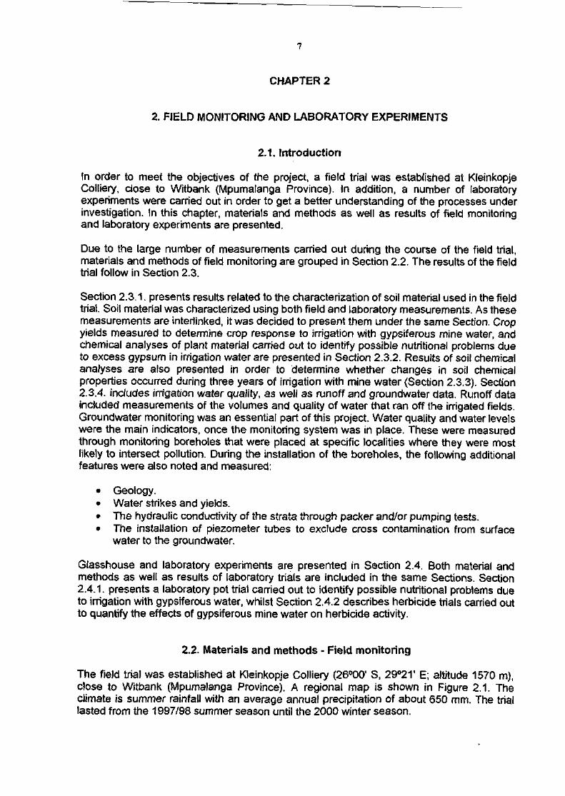
CHAPTER 2

2. FIELD MONITORING AND LABORATORY EXPERIMENTS

2.1. Introduction

In order to meet the objectives of the project, a field trial was established at KleinkopjeColliery, close to Witbank (Mpumalanga Province). In addition, a number of laboratoryexperiments were carried out in order to get a better understanding of the processes underinvestigation. In this chapter, materials and methods as well as results of field monitoringand laboratory experiments are presented.

Due to the large number of measurements carried out during the course of the field trial,materials and methods of field monitoring are grouped in Section 2.2. The results of the fieldtrial follow in Section 2.3.

Section 2.3.1. presents results related to the characterization of soil material used in the fieldtrial. Soil material was characterized using both field and laboratory measurements. As thesemeasurements are interlinked, it was decided to present them under the same Section. Cropyields measured to determine crop response to irrigation with gypsiferous mine water, andchemical analyses of plant material carried out to identify possible nutritional problems dueto excess gypsum in irrigation water are presented in Section 2.3.2. Results of soi! chemicalanalyses are also presented in order to determine whether changes in soil chemicalproperties occurred during three years of irrigation with mine water (Section 2.3.3). Section2.3.4. includes irrigation water quality, as well as runoff and groundwater data. Runoff dataincluded measurements of the volumes and quality of water that ran off the irrigated fields.Groundwater monitoring was an essential part of this project. Water quality and water levelswere the main indicators, once the monitoring system was in place. These were measuredthrough monitoring boreholes that were placed at specific localities where they were mostlikely to intersect pollution. During the installation of the boreholes, the following additionalfeatures were also noted and measured:

• Geology.• Water strikes and yields.• The hydraulic conductivity of the strata through packer and/or pumping tests.• The installation of piezometer tubes to exclude cross contamination from surface

water to the groundwater.

Glasshouse and laboratory experiments are presented in Section 2.4. Both material andmethods as well as results of laboratory trials are included in the same Sections. Section2.4.1. presents a laboratory pot trial carried out to identify possible nutritional problems dueto irrigation with gypsiferous water, whilst Section 2.4.2 describes herbicide trials carried outto quantify the effects of gypsiferous mine water on herbicide activity.

2.2. Materials and methods - Field monitoring

The field trial was established at Kleinkopje Colliery (26°00' S, 29°2f E; altitude 1570 m),close to Witbank (Mpumalanga Province). A regional map is shown in Figure 2.1. Theclimate is summer rainfall with an average annual precipitation of about 650 mm. The triallasted from the 1997/98 summer season until the 2000 winter season.

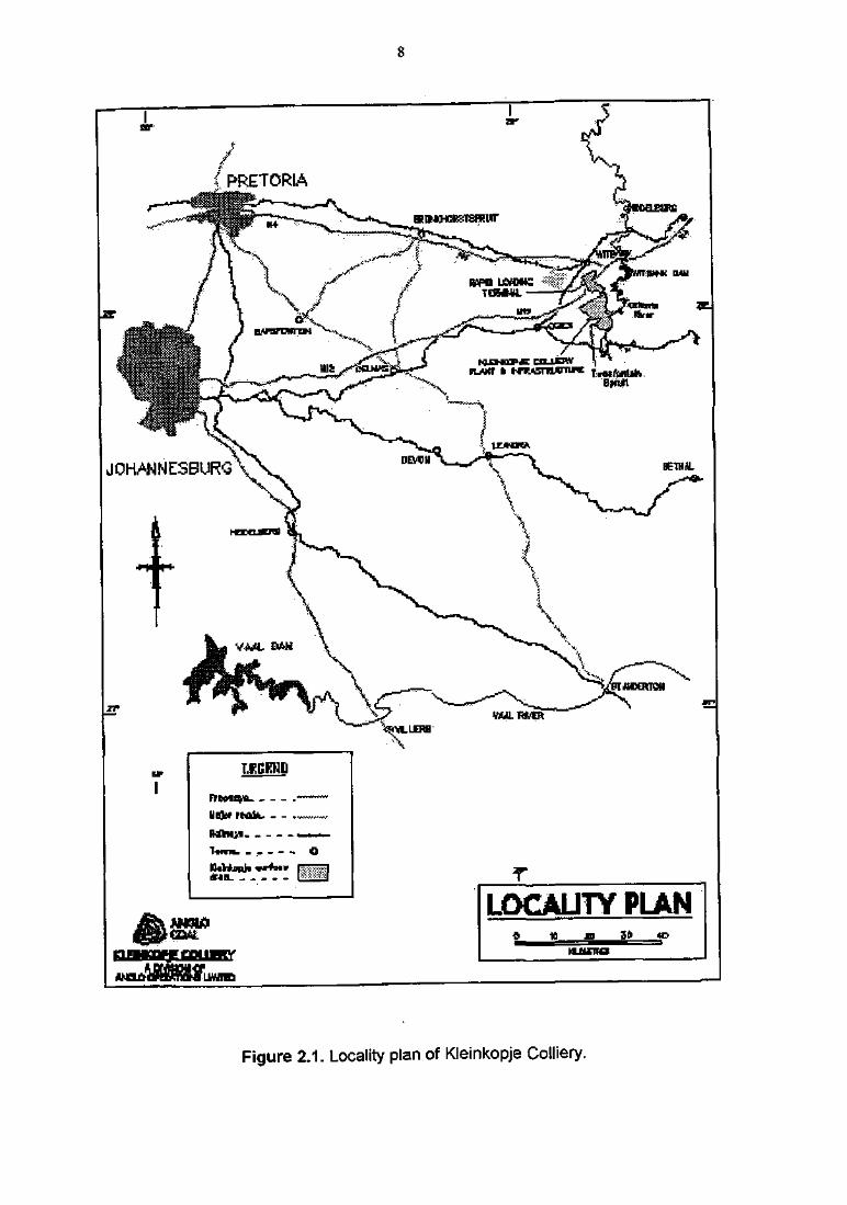
LOCAUTY PLAN

Figure 2.1. Locality plan of Kleinkopje Colliery.

2.2.1. Irrigation waters

Irrigations were carried out using two water qualities, namely Jacuzzi and Tweefontein.Jacuzzi water is pumped out of old underground workings and needs to be utilized byKleinkopje Colliery in order to enable mining operations to continue. Most of this water ispumped to a large storage dam and is released under controlled conditions under licencefrom the Dept. of Water Affairs and Forestry, Pretoria. Tweefontein water is pumped from anactive opencast pit and stored in the Tweefontein Pan.

2.2.2. Irrigation pivots

Four centre pivots were used for irrigation with gypsiferous mine water during the course ofthe trial:

• Pivot Major: Irrigated 30 ha of virgin (unmined) soil, predominantly Bainsvlei andClovelly (Soil Classification Working Group, 1991); Used Jacuzzi water for irrigation.

• Pivot Tweefontein: Irrigated 20 ha of rehabilitated soil; Used water from theTweefontein dam for irrigation.

• Pivot Jacuzzi: Irrigated 20 ha of rehabilitated soil from 1997 to 1999; Used Jacuzziwater for irrigation.

• Pivot Fourth: In autumn 1999, pivot Jacuzzi was moved to a virgin (unmined) site,due to problematic drainage at the rehabilitated site, and from then on, it was referredto as pivot Fourth. This was done to collect data for validation of the one-dimensionalSWB model at a well-drained site. One tower and an extension were added to thepivot, so that pivot Fourth irrigated 30 ha of Hutton soil (Soil Classification WorkingGroup, 1991) and used Tweefontein water for irrigation.

The mine map with the locations of the pivots, dams, plants, infrastructure and mining areasis shown in Figure 2.2.

Sugarbeans (Phaseolus vulgahs), maize (Zea Mays) and wheat (Triticum aestivum) weregrown during the course of the trial. Maize, babala (Pennisetum glaucum), stooling rye(Secale cereale), ryegrass (Lolium multiflorum) and a lucerne (Medicago sativa) - fescue(Festuca arundinacea) mixed perennial pasture were also grown under pivot Major on 0.5 halarge strips in order to test crop response and water use of alternative cropping systems.

Crops, cultivars, planting dates and agronomic techniques are summarized in Tables A1 toA4 (Appendix A) for each pivot. The lucerne-fescue pasture was fertigated according to therequirements of the main crop at pivot Major (Table A1, Appendix A).

From winter 1998, contours and waterways were shaped before the beginning of eachcropping season in order to facilitate drainage of excess water from the cultivated fields atpivots Major and Tweefontein.

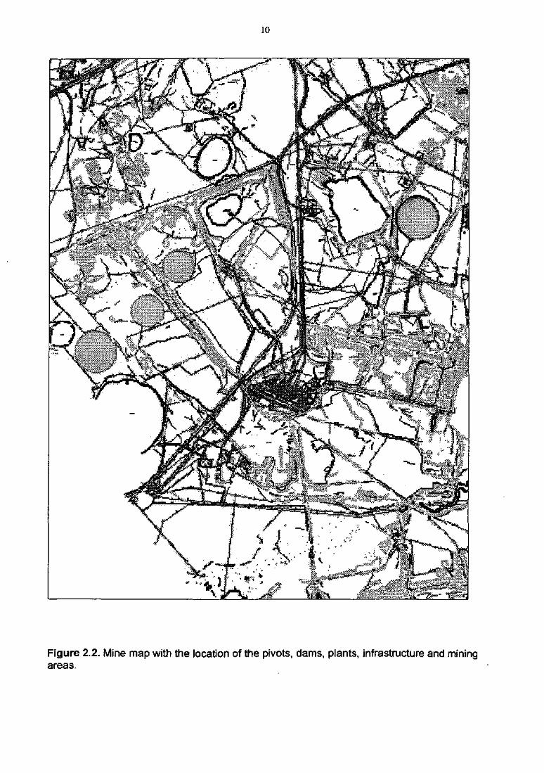
10

t ? •?&&••]

Figure 2.2. Mine map with the location of the pivots, dams, plants, infrastructure and miningareas.

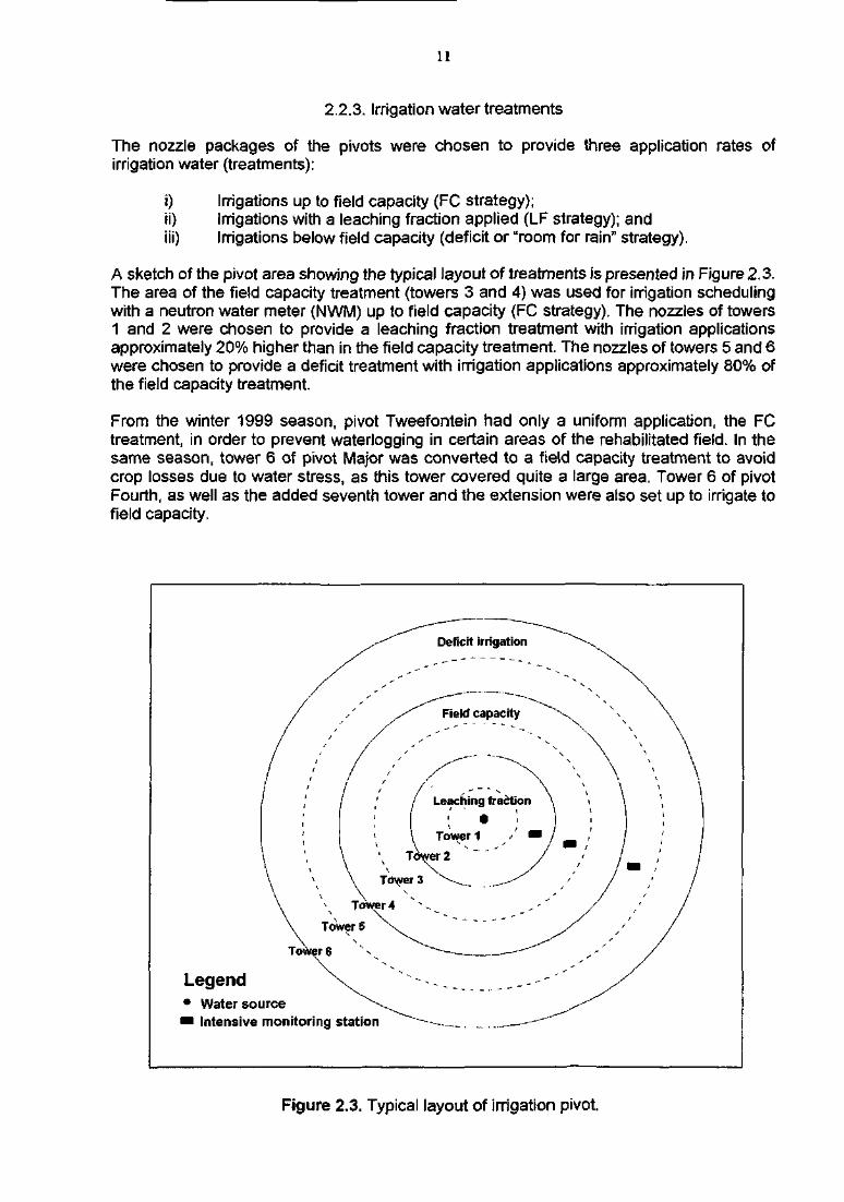
11

2.2.3. Irrigation water treatments

The nozzle packages of the pivots were chosen to provide three application rates ofirrigation water (treatments):

i) Irrigations up to field capacity (FC strategy);ii) Irrigations with a leaching fraction applied (LF strategy); andiii) Irrigations below field capacity (deficit or "room for rain" strategy).

A sketch of the pivot area showing the typical layout of treatments is presented in Figure 2.3.The area of the field capacity treatment (towers 3 and 4) was used for irrigation schedulingwith a neutron water meter (NWM) up to field capacity (FC strategy). The nozzles of towers1 and 2 were chosen to provide a leaching fraction treatment with irrigation applicationsapproximately 20% higher than in the field capacity treatment. The nozzles of towers 5 and 6were chosen to provide a deficit treatment with irrigation applications approximately 80% ofthe field capacity treatment.

From the winter 1999 season, pivot Tweefontein had only a uniform application, the FCtreatment, in order to prevent waterlogging in certain areas of the rehabilitated field. In thesame season, tower 6 of pivot Major was converted to a field capacity treatment to avoidcrop losses due to water stress, as this tower covered quite a large area. Tower 6 of pivotFourth, as well as the added seventh tower and the extension were also set up to irrigate tofield capacity.

Leaching fraction

Tower 1

Legend* Water source• Intensive monitoring station

Figure 2.3. Typical layout of irrigation pivot.

12

2.2.4. Atmospheric measurements

An automatic weather station was set up on 27/10/1997, at a location adjacent to pivotJacuzzi, approximately 100 m from the cropped area. In June 1999, before the beginning ofthe winter season when pivot Jacuzzi was moved to become pivot Fourth, the weatherstation was also moved to a location adjacent to pivot Tweefontein, approximately 100 mfrom the cropped area. Both sites where the weather station was set up, were surrounded bygrass and on a slight slope. The sites were assumed to be representative for the area wherethe three pivots were located.

The following data were recorded with the weather station:

Temperature and relative humidity with a CS-500 Vaisala temperature andhumidity probe;Solar radiation with a Li-Cor Ll-200 pyranometer;Wind speed with an R.M. Young cup anemometer; andRainfall amount and intensity with a tipping bucket Texas Electronics Inc. raingauge.

Weather data were recorded every 10 s with a Campbell Scientific CR10 data logger.Temperatures were averaged hourly, as well as averaged, maximized and minimized daily.Daily average, maximum and minimum relative humidity were recorded. The data loggerprogram was set up to calculate and output hourly and daily average vapour pressure andsaturation vapour pressure. Solar irradiance was averaged hourly and total daily radiant fluxdensity calculated. Wind speed was averaged, maximized and minimized daily.

Rainfall, if occurring, was recorded every minute in order to determine intensity, and totalisedhourly and daily. Rainfall recorded with the weather station could have been very differentfrom the rainfall occurring at the locations of the pivots. For this reason, intensive soilmonitoring stations at the pivots were provided with tipping bucket rain gauges (see followingSection 2.2.5. on intensive soil monitoring stations).

All sensors were regularly calibrated. Data recorded with the weather station were used asinput in the SWB model.

2.2.5. Soil measurements

Intensive monitoring stations were established under the pivots for measurement of thewater and salt balance in the soil profile. The purpose was to collect data for validation of theone-dimensional SWB model. Representative locations were chosen for each treatment inareas as flat as possible to minimize lateral movement of soil water.

The intensive monitoring stations included the following instrumentation:

i) Tipping bucket rain gauges for measurement of amount and intensity ofrainfall and irrigation. Rainfall and irrigation, if occurring, were recorded everyminute and totalised hourly and daily,

ii) Heat dissipation sensors (HDS) for measuring soil matric potential. Data wererecorded every 15 min or hourly, and sampled at the end of the day withCampbell Scientific CR10X data loggers,

iii) CS-615 soil water reflectometers for measuring volumetric soil water content.Data were recorded every 15 min, averaged hourly, and sampled at the endof the day with Campbell Scientific CR10X data loggers,

iv) Neutron probe access tubes for monitoring volumetric soil water content witha NWM, every 0.2 m down to 1.4 m. Readings were taken weekly.

13

v) Time domain reflectometry (TDR) probes for monitoring volumetric soil watercontent and bulk soil electrical conductivity with a Campbell ScientificTDR100 system. Readings were taken every hour.

vi) Ceramic cup soil water samplers to extract soil water samples for laboratoryanalyses.

vii) Automated tensiometer nests, comprising a logger and three or fourtensiometers, to determine the direction and magnitude of the hydraulicgradients and ultimately to verify detailed modelling of the liquid fluxes(Appendix B).

The treatments, instrumentation used, depths of installation and the description of the soilprofile where the instrumentation was installed are summarized in Tables A5 to A8(Appendix A) for each pivot and season.

During the first cropping season (summer 1997/98), the dry land area outside pivot Majorwas monitored as a control, both for the main crop (sugarbeans) and for the alternativecropping systems (babala and maize) (Table A5, Appendix A).

Two neutron probe access tubes per crop and treatment were installed in the alternativecropping systems plot of pivot Major during the 1997/98 summer season (babala and maize)and during the 1998 winter season (ryegrass and stooling rye). Soil water content readingswith the NWM were taken weekly. Irrigations and rainfall were recorded with manual raingauges for each treatment (LF, FC, deficit and dry land).

Two neutron probe access tubes per treatment were also installed in the wheat crops (1998,1999 and 2000 winter season) and maize crop (1999/2000 summer season) at pivot Major,Soil water content readings with the NWM were taken weekly. Irrigation and rainfall amountsand intensities were measured in the intensive monitoring stations of the lucerne-fescueperennial pasture for wheat and maize.

From winter 1999, the nozzle package of pivot Tweefontein was replaced to apply uniformamounts of water along its radius (FC strategy, Table A6, Appendix A). This limited thewaterlogging and crop losses, which were experienced in some areas of the LF treatment inthe previous summer cropping seasons.

Pivot Jacuzzi operated only from summer 1997/98 until summer. 1998/99 (Table A7,Appendix A). Before the beginning of the 1999 winter season, pivot Jacuzzi was removedfrom its original location to a virgin land site next to the Tweefontein dam (KleinkopjeColliery). The soil is Hutton (Soil Classification Working Group, 1991) with good drainageproperties. The main reason for the removal of the pivot was to collect field data at a well-drained site where lateral drainage is negligible. The original location of pivot Jacuzzi was onrehabilitated land, where lateral drainage was an important component of the soil water andsalt balance. Lateral drainage could only be modelled with a two- or three-dimensionalmodel. One of the main objectives of this project was to validate the SWB model in itspresent one-dimensional form.

From the winter 1999 season, and following the visit of Prof DR Nielsen (University of Davis,California) and the workshop on "Sampling field soils and their vegetation" held at theUniversity of Pretoria on the 24-25/07/1999, it was decided to move the remainingequipment from pivot Major to pivot Fourth in order to get replications and account for spatialvariability in measuring the soil water and salt balance. Six intensive soil monitoring stationswere established at pivot Fourth, along a diameter transect. Two stations were set up ineach treatment (Table A8, Appendix A).

14

2.2.6. Irrigation water chemical analyses

Irrigation water samples were collected in winter 1998 for chemical analyses at the SoilScience Laboratory (University of Pretoria). The samples were collected from the pivotnozzles. The irrigation water was analysed for concentrations of Ca2+, Mg2+, K+, Na+, SO4

2'and CI'. Electrical conductivity and pH were also measured. Irrigation water samples werealso collected and analysed by Kleinkopje Colliery at regular intervals. The results ofirrigation water chemical analyses are presented in Section 2.3.4.1.

2.2.7. Characterization of soil material

The soil profiles at the intensive monitoring stations were described and classified. Dry bulkdensities were determined with a variety of methods (Appendix C), whilst texture wasdetermined by sieving and with the hydrometer method.

The physical, hydraulic and solute transport characteristics of the soils and disturbedmaterials were determined for each of the pivots. Characterization of the soils served threepurposes:

i) The soil characteristics were used to describe the general behaviour of the waterin the profiles prior to modelling;

ii) The measured characteristics were used as initial model inputs to simulate thephysics and chemistry of liquid and solute movement in and below the root-zone;and

iii) Characteristics measured at different times were used to evaluate specificphenomena in the porous media, such as changes to pore structure due togypsum precipitation. Specific laboratory experiments were also conducted toaccelerate gypsum precipitation so that the pore structure changes could beevaluated without resorting to long-term in situ measurements.

The method of soil hydraulic characterization involved both in situ and laboratorymeasurements. A consistent procedure was adopted, wherever possible, for characterizingthe soil profiles investigated.

Firstly, at each level in the profile, a duplicate set of measurements was made. Themeasurements included an in situ tension infiltrometer test, followed by a double ringinfiltrometer test on exactly the same location. Secondly, an undisturbed core was takenfrom the precise site of the tension infiltrometer and double ring tests for laboratorydetermination of water retention characteristics and bulk density. The specific methodsemployed in developing the characteristics of the porous media are summarized in AppendixC. Detailed descriptions of conventional methods are not included here, except where themethods used in this study differ from convention.

A series of 300 mm deep by 110 mm diameter columns were packed with soil from pivotMajor in order to accelerate the gypsum precipitation process with loadings of approximately8, 30, 75 and 90 ton gypsum ha"1. A saturated solution was fed into the column intermittently.A vacuum pump was used to draw air through the pore spaces in the column between thecycles of gypsum solution inflow in order to enhance the precipitation of gypsum and toensure that the gypsum precipitated throughout the column as it would in a root-zone in thefield. A series of qualitative observations and a few quantitative estimates of the effect of thegypsum on the soil pore system were performed.

15

2.2.8. Soil analyses

Soil samples were collected before the beginning of the trial in the soil profiles from eachpivot and treatment area. The following parameters were determined for 0.2 m soil layersdown to 1 m:

Bulk density;Volumetric soil water content at -10 and -1500 J kg'1 soil matric potential;Concentrations of soluble Ca2+, Mg2+, K+, Na+, NH/ , SO/", CI", NCV, HCO3"and CO3

2';Concentrations of exchangeable Ca2 \ Mg2+, K+ and Na+; andBray I P.

In addition, soil pH(H2O) and electrical conductivity of the saturated soil extract (ECe) weredetermined.

Soil samples were also collected at the beginning of each season in the soil profiles fromeach pivot and treatment area. The following parameters were determined for 0.2 m soillayers down to 1 m;

Concentrations of Ca2+, Mg2+, K+, Na+, NH4+, SO/", Cr, NO3", HCCV and

CO32-;

Concentrations of exchangeable Ca2+, Mg2+, K+ and Na+;Soil pH(H2O);Electrical conductivity of the saturated soil extract; andBray I P.

These data were essential for the initial input settings of the SWB model, and for fertilizationrecommendations.

Water analyses were carried out on samples of soil water collected with the ceramic cup soilwater samplers. These samples were analysed for concentrations of Ca2+, Mg2+, K+, Na+,SO4

2' and CI". Electrical conductivity and pH were also measured. The purpose was tocompare these measurements to model predictions. Due to difficulties encountered inextracting soil water with the ceramic cup soil water samplers, particularly under dryconditions, soil samples were taken on 19/10/1998 in the deficit irrigation treatments of thewheat crop at all three pivot sites for laboratory analyses.

Deep soil sampling was carried out before the beginning of the winter 2000 season (June2000). This was done in order to explore whether any salt breakthrough originating fromirrigation could be identified in the vadose zone between the root-zone and the groundwater.Deep soil samples were collected from pivots Major, Fourth and Tweefontein. A geologicaldrill rig fitted with a 100 mm diameter push-tube soil corer was used to obtain completecores of soil from surface to a depth of 4.5 m in each of the irrigation treatment areas, and inan area just outside each of the three pivots, the latter samples being intended to representsoil not exposed to irrigation with gypsiferous mine water. Each soil core was divided in 200to 300 mm long sub-samples and bagged. The samples were air dried and analysed by theDepartment of Geology (University of Cape Town) and by the Soil Science Laboratory(University of Pretoria). Replicate sub-samples were analysed at both laboratories fordouble-checking purposes.

2.2.9. Measurement of precipitated gypsum

Precipitated gypsum was measured on deep soil samples collected in June 2000 for eachpivot and treatment block, as well as outside the pivot areas. Measurements of precipitated

16

gypsum were carried out on replicate sub-samples both at the Soil Science Laboratory(University of Pretoria) and at the Department of Geology (University of Cape Town). In thisSection, the methods used for measurement of precipitated gypsum are presented.

So/7 Science Laboratory (University of Pretoria)

Because of the low solubility of gypsum in water, the biggest problem with most of thegypsum determination methods is to determine the right soil to solution ratio in which all thegypsum in the soil will dissolve. This has lead to mostly lengthy and laborious methods. Theother drawback of gypsum analysis methods is that these methods have been developedmostly for taxonomical purposes, and not to obtain quantitative data. A brief overview of themethods found in the literature to determine soil gypsum content is given in Appendix D.After evaluation of all methods, it was decided to adapt the methods of Bower and Huss(1948) and the U.S. Soil Conservation Service (1972). This method is referred to as theAdapted Dilution Method (ADM). In this method, the low solubility of gypsum was anadvantage rather than a drawback and it was used to distinguish between gypsum and othersulphates, especially magnesium sulphates.

Department of Geology (University of Cape Town)

The research conducted at the Department of Geology (University of Cape Town) wasintended to supplement our knowledge of the potential of the soils of the MpumalangaHighveld to serve as repositories for the salts dissolved in saline mine water. In particular,this study had two aims: firstly, to assess whether the method used by Campbell (2001) todetect gypsum in soils - i.e. the analysis of the ionic composition of saturated paste extractsand the calculation of the gypsum saturation index (SI) - is reliable, and, secondly, to studythe capacity of the soils currently under irrigation with mine water at Kleinkopje to adsorbsulphate ions. The methodology and results for gypsum precipitation obtained at theDepartment of Geology (University of Cape Town) are given in Appendix E. The first part ofthis Appendix deals with the gypsum detection method and the second part with sulphateadsorption.

2.2.10. Evaluation of changes in soil salinity distribution on the irrigated areas

Establishment of changes in the spatial distribution of soil salinity with time was based onsurveys conducted using the electromagnetic induction (EM) technique. The EM-38 sensorof Geonics Ltd (Ontario) makes rapid measurements of soil EC and has been shown toprovide a cost-effective method to map soil salinity distribution (Rhoades, 1992; McKenzie etal., 1989; Johnston et al., 1994). Measurements can be made with the sensor positionedeither in the horizontal (EMh) or vertical (EMV) position. In the former position the response isprimarily from the upper soil profile (64% of the response arises from the upper 60 cm), whilein the vertical position the instrument is more responsive to the deeper layers (only 36%attributed to the upper 60 cm). Interpretation of the measurements is greatly enhanced bycalibration during each survey of the EM values with the ECe of soil samples taken down theprofile (Johnston et al., 1997). From a limited number of observation points a regressionrelationship can be established that allows the prediction of ECe from the numerous EMmeasurements that are made over the whole survey area.

Each year since 1997 a survey has been conducted at the different centre pivots. The EM-38 sensor has been used to obtain field measurements of EMV and EMh These have beencorrected to a standard temperature of 25°C, as recommended by McKenzie et al. (1989),based on soil temperature at a depth of 45 cm. From these values the mean of the EMV andEMh (i-6- EMmean) was determined. The salinity surveys have increased in their sophisticationover the period of this project, partly due to new equipment that has become available. Thisrelates mainly to the use of a G.P.S. receiver. The measurement positions were, during

17

1997-1999, located at points on a grid. This 40 X 80 m (or 40 X 40 m) grid had to be peggedout manually, which was a laborious and time-consuming exercise. The SURFER graphicspackage (Golden Software Inc.) was used in 1998 and 1999 to plot salinity contours. InDecember 2000 the G.P.S. (Trimble model TSC1) was used to provide accurate (< 1.0 m)positions of measurement points at spacings of between 25 and 50 m on three centre pivots(Major, Tweefontein and Fourth). This allowed for a faster and more appropriate procedure.In that geographic co-ordinates were being recorded, the ArcView G.I.S. package could beused to process the data and produce salinity contours using the "Kriging" statistical option.During each survey, soil samples were taken at 30 cm intervals down the profile fromdominant soil types on each pivot for saturation extract analysis. A regression relationshipwas then established between ECe (0-60 cm) and EMmean-

2.2.11. Runoff amounts and quality

During winter 1999, runoff crump weirs were built at the bottom of the waterways at pivotMajor and Tweefontein. The depth of water overflowing the weirs was measured with apressure transducer connected to a CR-510 data logger. This was then used to determinethe amount of water overflowing the weir. Electrical conductivity of runoff water was alsomeasured with a salinity sensor connected to the CR-510 data logger. Data were recordedevery 2 min only during runoff events (weir overflowing). The data collected at the weirswere used to quantify the amount of water and salts running off the irrigated areas at pivotsMajor and Tweefontein.

2.2.12. Installation of monitoring boreholes

2.2.12.1. Siting of the boreholes

A budget was provided by the mine for nine monitoring boreholes at pivot Major. These werespaced as indicated in Figure 2.4.

The surface slope through the irrigation area is to the South-West at an average gradient of1:30.

Borehole 1 was intended to monitor virgin conditions, but it collapsed soon after installation.Boreholes 2 - 7 are spaced on a West to East line, approximately coinciding with the 1 560m contour across the irrigation area. Boreholes 8 and 9 are located at the lowest surfacepositions.

The holes were all drilled to a depth of 15 m. This shallow depth was necessitated by thepresence of underground mining of the No. 5 Seam Horizon (Figure 2.4), which could be asshallow as 20 m below the surface in some places.

2.2.12.2. Drilling

Drilling of the boreholes was done through air percussion drilling. The hole diameters are165 mm. Samples for geological logging were taken at 1 m intervals. The blowout yieldsfrom the boreholes were noted while drilling.

Considerable instability of the strata was encountered while drilling. Yields from theboreholes were very low, but sufficient to cause additional instability in the holes once waterwas intersected. This instability necessitated a change in test procedures. It was intended toperform packer, pumping and slug tests on the boreholes to determine the hydrauliccharacteristics of the strata. The collapse of the boreholes was so severe that piezometershad to be installed immediately after each borehole was drilled.

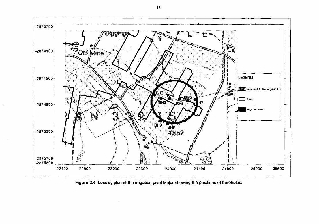
18

-2873700 i

-2874100^

-2874500-

-2874900-

-2875300

-2875700--2875800

LEGEND

Landau 5 S Underground

i 1 Dam

Irrigation area

22400 22800 23200 23600 24000 24400 24800 25200 25600

Figure 2.4. Locality plan of the irrigation pivot Major showing the positions of boreholes.

19

2.2.12.3. Geology and geohydrology

The geology of the area is relatively homogeneous. It consists of 2 - 5 m soil, followed bysandstone. The sandstone is highly weathered to depths of 10 - 12 m. Below this depth, thesandstone is fresh with a white appearance. A typical geological profile is shown in Figure2.5. Complete geological logs for each of the boreholes are presented in Appendix F.

Water, in small quantities, was intersected in all boreholes in the weathered sandstone.

2.2.12.4. Piezometer installation

A piezometer consists of a slotted PVC tube, 62.5 mm in diameter, which is installed in aborehole for the purpose of measuring and sampling at specific elevations.

The purpose of piezometer installation in each of the monitoring boreholes was two-fold. Inthe first instance, the piezometer tubes serve to keep the holes from collapsing. Secondly,they effectively seal the holes in the vertical dimension, thus preventing surface water fromflowing into the holes. A typical piezometer design is demonstrated in Figure 2.6. Details ofpiezometer installations in all the boreholes are provided in Appendix.F.

2.2.12.5. Hydraulic characteristics of the aquifer

Due to the collapsing nature of the strata, hydraulic tests could not be performed beforepiezometer installation. As a result, pumping tests had to be performed with a small diameterpump, which was lowered into the piezometer tubes. The pumping test curves are includedin Appendix G. Table 2.1 summarizes the results from the pumping tests.

The calculated transmissivities are low and incapable of sustaining prolonged groundwaterabstraction. Nevertheless, hydraulic conductivity is high enough for water on the surface topenetrate into the sediments below. Water will move vertically to a depth of 10 - 12 m,whereafter it will move laterally on top of the fresh sandstone. The hydraulic gradient istowards South-West, i.e. in the direction of the stream.

Noticeable is the higher transmissivity of the strata at BH5 and the associated deeper staticgroundwater level. This suggests a lateral hydraulic connection, which allows drainage ofgroundwater from this area.

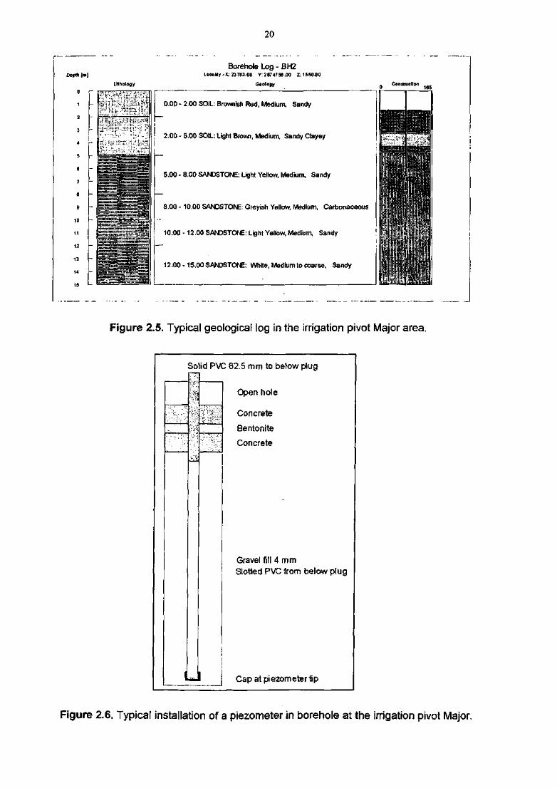
20

DepBilm

0

1

2

3

4

5

e

7

a

e

10

11

12

13

14

15

Ulhology

Borehole Log - BH2LoiaMy.)t2J7B3.O0 Y;28747S6.00 Z:1560H0

Gsotopy

0.00-2.00 SOIL: BTOvmish Red, Mediunn, Sandy

2.00 - 5.00 SOIL: Lighl BIOVJCX, Medium, Sandy Clayey

S.OO - 8.00 SANDSTONE: Light Yellow, Medium, Sandy

8.00 -10.00 SANDSTONE: Greyish Yellow, Medium, Carbonaceous

10.00 -12.00 SANDSTONE: Light Yellow, Medium, Sandy

12.00-1S.O0 SANDSTONE: White, Medium to coarse, Sandy

Figure 2.5. Typical geological log in the irrigation pivot Major area.

Solid PVC 62.5 mm to below plug

Open hole

Concrete

Bentonite

Concrete

Gravel fill 4 mmSlotted PVC from below plug

I-J i Cap at piezometer lip

Figure 2.6. Typical installation of a piezometer in borehole at the irrigation pivot Major.

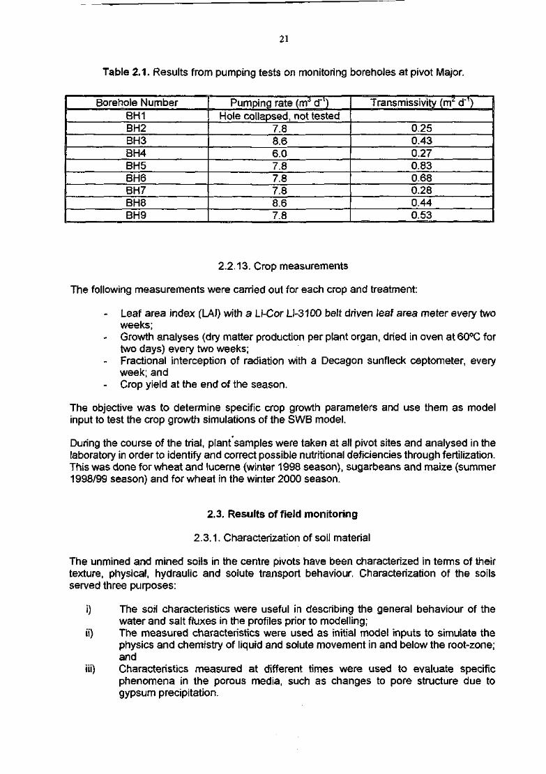
21

Table 2.1. Results from pumping tests on monitoring boreholes at pivot Major.

Borehole NumberBH1BH2BH3BH4BH5BH6BH7BH8BH9

Pumping rate (m3 d"1)Hole collapsed, not tested

7.88.66.07.87.87.88.67.8

Transmissivity (m2 d"1)

0.250.430.270.830.680.280.440.53

2.2.13. Crop measurements

The following measurements were carried out for each crop and treatment:

- Leaf area index (LAI) with a Li-Cor LI-3100 belt driven feaf area meter every twoweeks;

- Growth analyses (dry matter production per plant organ, dried in oven at 60°C fortwo days) every two weeks;Fractional interception of radiation with a Decagon sunfleck ceptometer, everyweek; and

- Crop yield at the end of the season.

The objective was to determine specific crop growth parameters and use them as modelinput to test the crop growth simulations of the SWB model.

During the course of the trial, plant samples were taken at all pivot sites and analysed in thelaboratory in order to identify and correct possible nutritional deficiencies through fertilization.This was done for wheat and lucerne (winter 1998 season), sugarbeans and maize (summer1998/99 season) and for wheat in the winter 2000 season.

2.3. Results of field monitoring

2.3.1. Characterization of soil material

The unmined and mined soils in the centre pivots have been characterized in terms of theirtexture, physical, hydraulic and solute transport behaviour. Characterization of the soilsserved three purposes:

i) The soil characteristics were useful in describing the general behaviour of thewater and salt fluxes in the profiles prior to modelling;

ii) The measured characteristics were used as initial model inputs to simulate thephysics and chemistry of liquid and solute movement in and below the root-zone;and

iii) Characteristics measured at different times were used to evaluate specificphenomena in the porous media, such as changes to pore structure due togypsum precipitation.

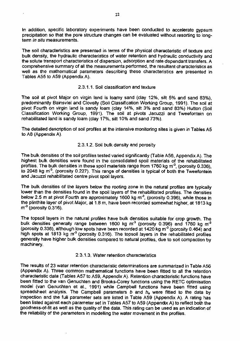
22

In addition, specific laboratory experiments have been conducted to accelerate gypsumprecipitation so that the pore structure changes can be evaluated without resorting to long-term in situ measurements.

The soil characteristics are presented in terms of the physical characteristic of texture andbulk density, the hydraulic characteristics of water retention and hydraulic conductivity andthe solute transport characteristics of dispersion, adsorption and rate dependant transfers. Acomprehensive summary of all the measurements performed, the resultant characteristics aswell as the mathematical parameters describing these characteristics are presented inTables A55 to A59 (Appendix A).

2.3.1.1. Soil classification and texture

The soil at pivot Major on virgin land is loamy sand (clay 12%, silt 5% and sand 83%),predominantly Bainsvlei and Clovelly (Soil Classification Working Group, 1991). The soil atpivot Fourth on virgin land is sandy loam (clay 14%, silt 3% and sand 83%) Hutton (SoilClassification Working Group, 1991). The soil at pivots Jacuzzi and Tweefontein onrehabilitated land is sandy loam (clay 17%, silt 10% and sand 73%).

The detailed description of soil profiles at the intensive monitoring sites is given in Tables A5to A8 (Appendix A).

2.3.1.2. Soil bulk density and porosity

The bulk densities of the soil profiles tested varied significantly (Table A56, Appendix A). Thehighest bulk densities were found in the consolidated spoil materials of the rehabilitatedprofiles. The bulk densities in these spoil materials range from 1760 kg m"3, (porosity 0.336),to 2048 kg m"3, (porosity 0.227). This range of densities is typical of both the Tweefonteinand Jacuzzi rehabilitated centre pivot spoil layers.

The bulk densities of the layers below the rooting zone in the natural profiles are typicallylower than the densities found in the spoil layers of the rehabilitated profiles. The densitiesbelow 2.5 m at pivot Fourth are approximately 1600 kg m'3, (porosity 0.396), while those inthe piinthite layer of pivot Major, at 1.8 m, have been recorded somewhat higher, at 1813 kgrrT3 (porosity 0.316).

The topsoil layers in the natural profiles have bulk densities suitable for crop growth. Thebulk densities generally range between 1600 kg m~3 (porosity 0.396) and 1760 kg m"3

(porosity 0.336), although low spots have been recorded at 1420 kg m"3 (porosity 0.464) andhigh spots at 1813 kg m'3 (porosity 0.316). The topsoil layers in the rehabilitated profilesgenerally have higher bulk densities compared to natural profiles, due to soil compaction bymachinery.

2.3.1.3. Water retention characteristics

The results of 23 water retention characteristic determinations are summarized in Table A56(Appendix A). Three common mathematical functions have been fitted to all the retentioncharacteristic data (Tables A57 to A59, Appendix A). Retention characteristic functions havebeen fitted to the van Genuchten and Brooks-Corey functions using the RETC optimisationmodel (van Genuchten et al,, 1991) while Campbell functions have been fitted usingspreadsheet analysis. The Campbell parameters b and he were fitted to the data byinspection and the full parameter sets are listed in Table A59 (Appendix A). A rating hasbeen listed against each parameter set in Tables A57 to A59 (Appendix A) to reflect both thegoodness-of-fit as well as the quality of the data. This rating can be used as an indication ofthe reliability of the parameters in modelling the water movement in the profiles.

23

Typical ranges of water retention characteristics for four locations at pivot Major are shownin Figure 2.7 for the surface layer, and in Figure 2.8 for materials sampled at 0.5 m belowsurface. The Campbell mathematical function was fitted to the data for the upper and lowerrange of retention characteristics, which define the envelope of the distribution of data. Theretention characteristic curve fitted to the data with the larger water content for a givencapillary pressure head (Major 1 in Figures 2.7 and 2.8} is called the upper bound. Theretention characteristic curve fitted to the data with the lower water content (Major 3 in Figure2.7 and Major 4 in Figure 2.8) is called the lower bound. These fitted characteristics,therefore, define the limits of the range of water retention parameters that would be used in asensitivity study of modelled soil water dynamics.

Both these sets of retention characteristics show a significant loss of liquid at low matricpressure heads (below 2 m), reflecting a loose structure and the presence of a significantvolume of large pore sizes and, thus, a low Drained Upper Limit (DUL). However, thisvolume of large pore sizes is greater for the surface samples than for those at 0.5 m. Theresidual water content at a matric pressure head of 20 m (2 bar), ranges between 0.05 and0.12 for the samples at 0.5 m, while on the surface this residual water content is narrowlydistributed between 0.03 and 0.05. The spatial variation in water retention characteristicappeared to be greater at 0.5 m than at the surface, where the materials have probably beenmore disturbed through the tilling processes.

The water retention characteristic for the plinthite material at pivot Major is shown in Figure2.9. The porosity of this material (0.31) is lower than the porosities found in the surface andnear surface soils (0.35 - 0.45). The residual water content at 20 m matric pressure head(0.18) is also greater than any recorded for the upper layers.

The water retention characteristics for a typical topsoi! and spoil sample are shown for therehabilitated profile at pivot Tweefontein in Figure 2.10. The porosity is low (0.32) and theresidual water content at 2 m matric pressure head is high (0.18), indicative of thecompacted structure of the material.

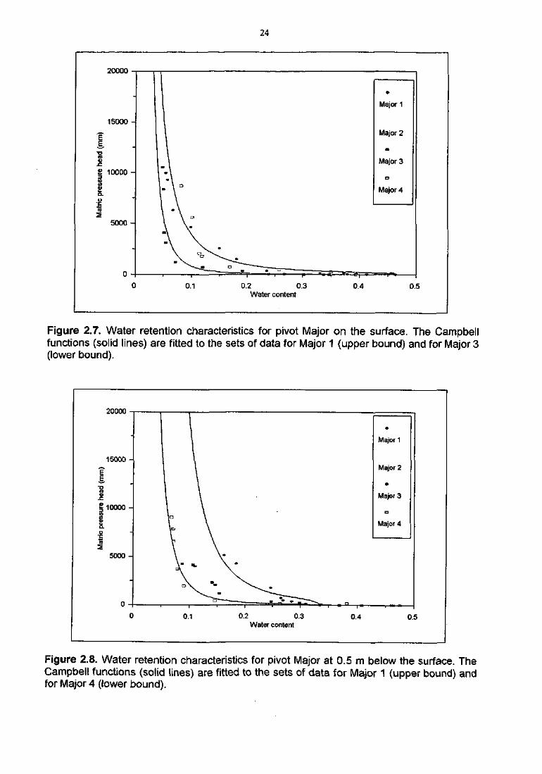
24

20000

15000 -

E

£ 10000

5000 -

0 -

0 0.2 0.3Water content

0.4

Major 1

Major 2

Major 3

Major 4

0.5

Figure 2.7. Water retention characteristics for pivot Major on the surface. The Campbellfunctions (solid lines) are fitted to the sets of data for Major 1 (upper bound) and for Major 3(lower bound).

''0000

mm

)ric

pre

ssur

e he

ad i

o o 8i

i

Mat

0 -

0

I

In

V

• \

0.1

\

0.2 0.3 0.4Water content

Major 1

Major 2

m

Major 3

•

Major 4

0 5

Figure 2.8. Water retention characteristics for pivot Major at 0.5 m below the surface. TheCampbell functions (solid lines) are fitted to the sets of data for Major 1 (upper bound) andfor Major 4 (lower bound).

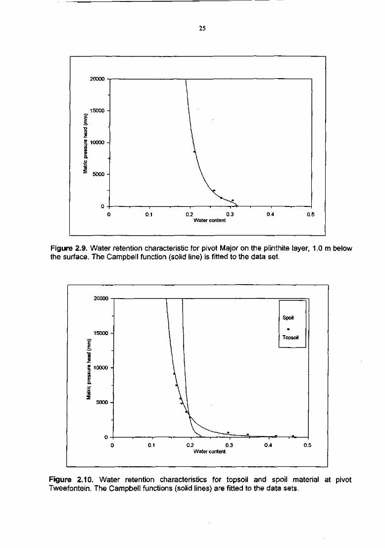
25

Figure 2.9. Water retention characteristic for pivot Major on the piinthite layer, 1.0 m belowthe surface. The Campbell function (solid line) is fitted to the data set.

9nnnn

15000 -

£•aIB

£ 10000 -•9

latric

pre

s

5000 -

0

1Spoil

Topsoil

I

1\

i | i | i | i | 1 •

0.1 0.2 0.3 0.4 0.5Water content

Figure 2.10. Water retention characteristics for topsoil and spoil material at pivotTweefontein. The Campbell functions (solid lines) are fitted to the data sets.

26

2.3.1.4. Hydraulic conductivity characteristics

The results of the saturated and unsaturated hydraulic conductivity measurements aresummarized in Table A56 (Appendix A) for all the pivots. The hydraulic conductivities of allprofiles, whether natural or disturbed, decreased with depth. Saturated hydraulicconductivities at the surface ranged typically from 5 mm h'1 and 500 mm h"1 with pivot Majorexhibiting the highest conductivities. A single measurement in the spoil layer at Jacuzziyielded a conductivity of 0.9 mm h'1, however the measurements of unsaturated hydraulicconductivity at 60 mm and 150 mm matric pressure head in the spoil were similar to those inthe topsoil profile.

Typical hydraulic characteristic curves were plotted for pivot Major, Jacuzzi and Tweefonteinin Figures 2.11 to 2.13. The mathematical functions derived by simultaneously optimizing thevan Genuchten characteristic functions to the water retention and hydraulic conductivity dataare also shown in Figures 2.11 to 2.13. The curves show the typical variation of hydraulicconductivity characteristic with depth. Parameters of the van Genuchten, Brooks-Corey andCampbell functions that have been simultaneously fitted to the retention and hydraulicconductivity data are summarized in Tables A57 to A59 (Appendix A).

In the rehabilitated profiles, the conductivity characteristic is high at low matric pressureheads (high saturation), typically between 10 and 100 mm IT1 (Figure 2.11 and 2.12).However, the characteristic curve drops off rapidly with conductivities decreasing two ordersof magnitude over a range of 1 m of matric pressure head. In the deeper spoil profiles theconductivities near saturation are low (between 1 and 10 mm h"1), but do not drop off asrapidly with increasing matric pressure head as those near the surface. Here theconductivities reduce by less than an order of magnitude over a change in matric pressurehead of 1 m. This behaviour reflects the loose structure of the near surface materials incontrast to the compacted structure of the deeper soil layers and spoil materials.

In the natural profile at pivot Major, the conductivity characteristic shapes are similar for thesurface and plinthite materials, but the plinthite conductivities are some two orders ofmagnitude smaller than those of the soil, both nearer the surface and at 0.85 m below thesurface (Figure 2.13). The soil/plinihite contact is therefore likely to conduct water easily,without ponding or inducing lateral movement of water at this interface.

In order to define the spatial variability of hydraulic characteristics, a set of 35 tensioninfiltrometer measurements were performed in a radial pattern at pivot Major. The average ofthe hydraulic conductivity measurements decreased with increased applied tension, whilethe range of the maximum and minimum of the hydraulic conductivity measurementsincreased with increased applied tension. The decrease of the average hydraulicconductivity was small, varying from 12.6 mm h'1 at an applied tension of 60 mm to 7.5 mmh"1 at 150 mm.

The spatial distribution of the hydraulic conductivity measurements is represented in Figure2.14 for the 60 mm tension and in Figure 2.15 for the 150 mm tension. While the range ofhydraulic conductivity values was high for the 150 mm measurements, the variabilityspatially was low, with most of the pivot area exhibiting conductivities between 6 and 8 mmh"1. The spatial variability of the measurements at 60 mm tension was larger than that for the150 mm tension measurements, however some 50% of the field had conductivities between8 and 14 mm h'1 at 60 mm tension.

Based on these results, it is clear that high bulk density due to soil compaction and thepresence of the spoil layer with low hydraulic conductivity are limiting factors for cropproduction under irrigation on rehabilitated land.

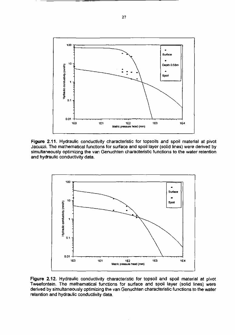
27

100 -3

_ 10 -

E

uct

ivity

8 ;ZJ

0 .1 •:

.

1E0

_ _ _ _

1E1

\

\

\

1E2Matric pressure head (mm)

\

\

1E3

Surface

•

Depth 0.55fn

Spoil

\

\

1E4

Figure 2.11. Hydraulic conductivity characteristic for topsoils and spoil material at pivotJacuzzi. The mathematical functions for surface and spoil layer (solid lines) were derived bysimultaneously optimizing the van Genuchten characteristic functions to the water retentionand hydraulic conductivity data.

Figure 2.12. Hydraulic conductivity characteristic for topsoil and spoil material at pivotTweefontein. The mathematical functions for surface and spoil layer (solid lines) werederived by simultaneously optimizing the van Genuchten characteristic functions to the waterretention and hydraulic conductivity data.

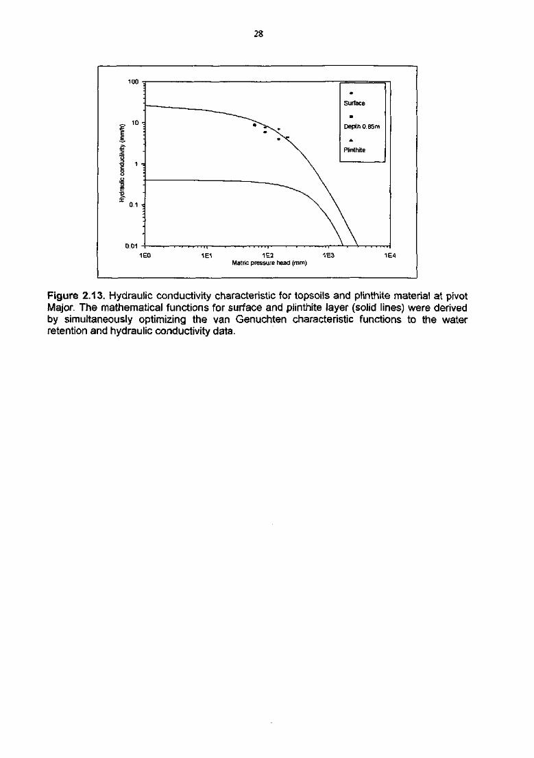
28

1Q0

10 -.

1 -.

0.1 •:

0.01

Surface

Depth 0.85m

Plinthite

1EO 1E1 1E2Matric pressure head (mm)

1E3 1E4

Figure 2.13. Hydraulic conductivity characteristic for topsoils and plinthite material at pivotMajor. The mathematical functions for surface and plinthite layer (solid lines) were derivedby simultaneously optimizing the van Genuchten characteristic functions to the waterretention and hydraulic conductivity data.

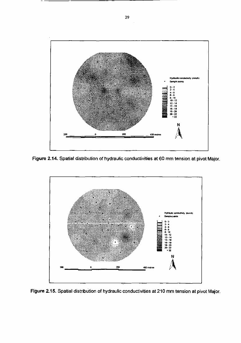
29

A «

c ccfiductt^ty (mroAi)

Sample points

0 - 22 - 44 - 66 - 68- 1010-1212-1414-1616-1618-2020-22

N

200

Figure 2.14. Spatial distribution of hydraulic conductivities at 60 mm tension at pivot Major.

, ' . - : - : • : : - : • : : : • : • : • : • : • : : • : • : - : - : • : • / : • : • : • : • : • : • : • • • : •*:•:-.-.. . - : • • : - : - : : ••:- : • : ••:• vs. '•• >:'.<•'.- >-•>: • ; • : • : • : • : • ; • : • ; • : • : : H X «

!:::;:::;:':;:!:^:::^:::-r-:::":Sy$>!-^'™^

^:S::-:::O: :: :: :: ::"5:S::S5SS:::WJ¥S-KSK-^^^^

'•'•:::;:^;::::::::H:Si;:s;j;SSg;^g¥s::;"'

20a 0 200

^ ^ f c H^raJ« mndudl̂ ly (n,m/h|

l i i i l l t : * ^p,.p*ts^ 1 H LJ *-*: .•:•.--•>; •:•;-:-:•:•:':• :•:•:$

:-:•:•:•>:•:-:•:-:->:-:-:•:-;-:

• - • ' • • > . 2 - 4

«SS 8-10Ks«-:-:*K-:-:jvC-W' .; ̂ . ; ; -

!?>::::?feo:SySf i ̂ ^ 12-14

i ^ i i P . ^ 14-ieWM&W ^ 16-18|ip;p- E ^ 18-20

N

4400 metres

Figure 2.15. Spatial distribution of hydraulic conductivities at 210 mm tension at pivot Major.

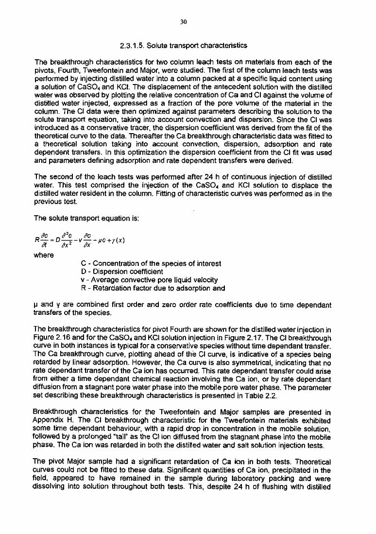
30

2.3.1.5. Solute transport characteristics

The breakthrough characteristics for two column leach tests on materials from each of thepivots, Fourth, Tweefontein and Major, were studied. The first of the column leach tests wasperformed by injecting distilled water into a column packed at a specific liquid content usinga solution of CaSO4 and KCI. The displacement of the antecedent solution with the distilledwater was observed by plotting the relative concentration of Ca and CI against the volume ofdistilled water injected, expressed as a fraction of the pore volume of the material in thecolumn. The CI data were then optimized against parameters describing the solution to thesolute transport equation, taking into account convection and dispersion. Since the CI wasintroduced as a conservative tracer, the dispersion coefficient was derived from the fit of thetheoretical curve to the data. Thereafter the Ca breakthrough characteristic data was fitted toa theoretical solution taking into account convection, dispersion, adsorption and ratedependent transfers. In this optimization the dispersion coefficient from the CI fit was usedand parameters defining adsorption and rate dependent transfers were derived.

The second of the leach tests was performed after 24 h of continuous injection of distilledwater. This test comprised the injection of the CaSO4 and KCI solution to displace thedistilled water resident in the column. Fitting of characteristic curves was performed as in theprevious test.

The solute transport equation is:

ndc ^d2c dcR D v

whereC - Concentration of the species of interestD - Dispersion coefficientv - Average convective pore liquid velocityR - Retardation factor due to adsorption and

u and Y are combined first order and zero order rate coefficients due to time dependanttransfers of the species.

The breakthrough characteristics for pivot Fourth are shown for the distilled water injection inFigure 2.16 and for the CaSO4 and KCI solution injection in Figure 2.17. The CI breakthroughcurve in both instances is typical for a conservative species without time dependant transfer.The Ca breakthrough curve, plotting ahead of the CI curve, is indicative of a species beingretarded by linear adsorption. However, the Ca curve is also symmetrical, indicating that norate dependant transfer of the Ca ion has occurred. This rate dependant transfer could arisefrom either a time dependant chemical reaction involving the Ca ion, or by rate dependantdiffusion from a stagnant pore water phase into the mobile pore water phase. The parameterset describing these breakthrough characteristics is presented in Table 2.2.

Breakthrough characteristics for the Tweefontein and Major samples are presented inAppendix H. The CI breakthrough characteristic for the Tweefontein materials exhibitedsome time dependant behaviour, with a rapid drop in concentration in the mobile solution,followed by a prolonged "tail" as the CI ion diffused from the stagnant phase into the mobilephase. The Ca ion was retarded in both the distilled water and salt solution injection tests.

The pivot Major sample had a significant retardation of Ca ion in both tests. Theoreticalcurves could not be fitted to these data. Significant quantities of Ca ion, precipitated in thefield, appeared to have remained in the sample during laboratory packing and weredissolving into solution throughout both tests. This, despite 24 h of flushing with distilled

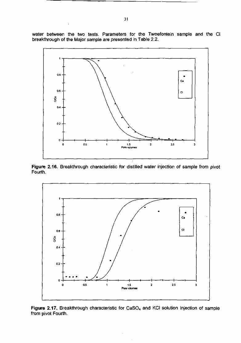
31

water between the two tests. Parameters for the Tweefontein sample and the Clbreakthrough of the Major sample are presented in Table 2.2.

1 "I

o.e -

0.6 -

0.4 -

o -

0 0.5

\

\ \

\ \

\

1 1.5Pors volumes

2

*

Ca

Cl

2.5 3

Figure 2.16. Breakthrough characteristic for distilled water injection of sample from pivotFourth.

0 . 8 - -

0 . 6 - -

8 -0,4 - -

0.2 - -

2.5

Figure 2.17. Breakthrough characteristic for CaSO4 and KCI solution injection of samplefrom pivot Fourth.

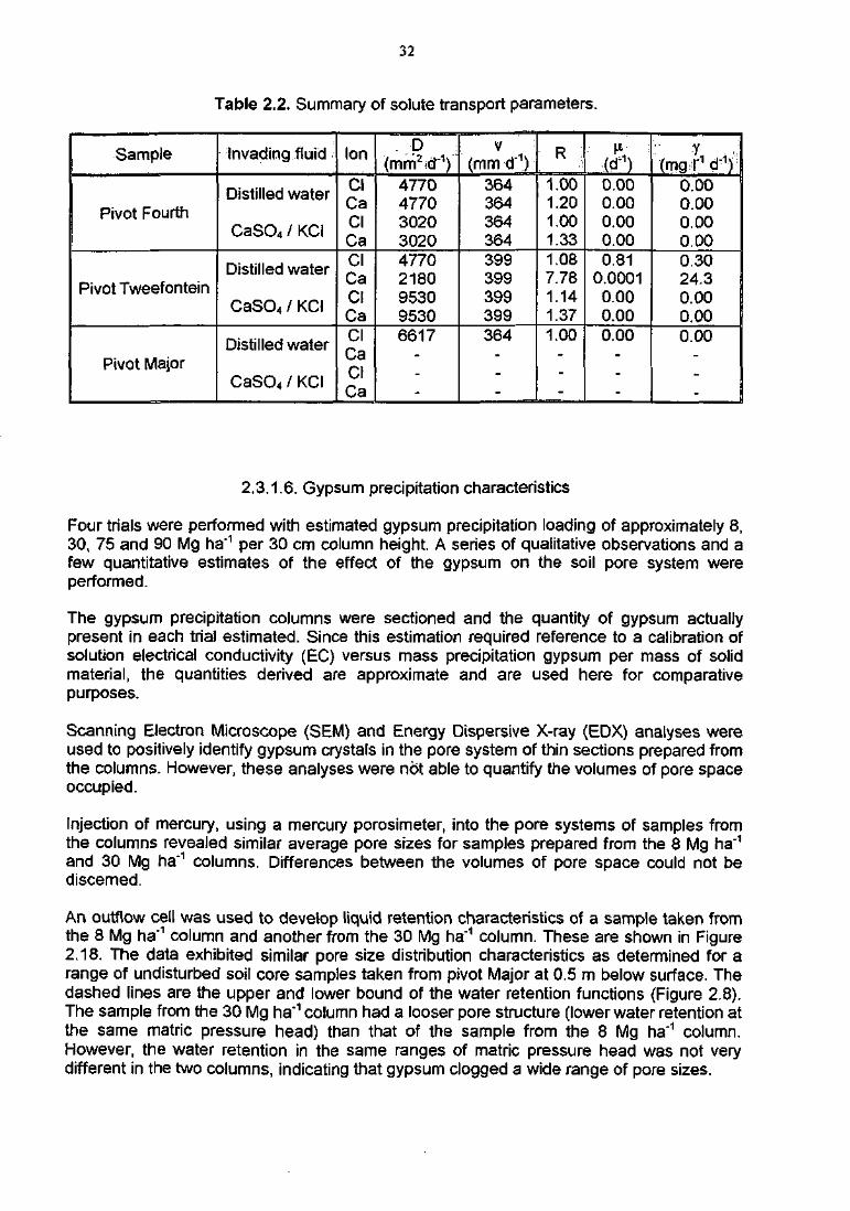
32

Table 2.2. Summary of solute transport parameters.

Sample

Pivot Fourth

Pivot Tweefontein

Pivot Major

Invading fluid

Distilled water

CaSO4 / KCI

Distilled water

CaSO4 / KCI

Distilled water

CaSCU / KCI

Ion

ClCaClCaClCaClCaClCaClCa

D(mm2 id'1)

477047703020302047702180953095306617

V

(mmd"1)364364364364399399399399364

: R i1.001.201.001.331.087.781.141.371.00

:(d'1)0.000.000.000.000.81

0.00010.000.000.00

;• r . J(mgl'1 tf1);

0.000.000.000.000.3024.30.000.000.00

2.3.1.6. Gypsum precipitation characteristics

Four trials were performed with estimated gypsum precipitation loading of approximately 8,30, 75 and 90 Mg ha"1 per 30 cm column height. A series of qualitative observations and afew quantitative estimates of the effect of the gypsum on the soil pore system wereperformed.

The gypsum precipitation columns were sectioned and the quantity of gypsum actuallypresent in each trial estimated. Since this estimation required reference to a calibration ofsolution electrical conductivity (EC) versus mass precipitation gypsum per mass of solidmaterial, the quantities derived are approximate and are used here for comparativepurposes.

Scanning Electron Microscope (SEM) and Energy Dispersive X-ray (EDX) analyses wereused to positively identify gypsum crystals in the pore system of thin sections prepared fromthe columns. However, these analyses were not able to quantify the volumes of pore spaceoccupied.

Injection of mercury, using a mercury porosimeter, into the pore systems of samples fromthe columns revealed similar average pore sizes for samples prepared from the 8 Mg ha"1

and 30 Mg ha'1 columns. Differences between the volumes of pore space could not bediscerned.

An outflow cell was used to develop liquid retention characteristics of a sample taken fromthe 8 Mg ha"1 column and another from the 30 Mg ha"1 column. These are shown in Figure2.18. The data exhibited similar pore size distribution characteristics as determined for arange of undisturbed soil core samples taken from pivot Major at 0.5 m below surface. Thedashed lines are the upper and lower bound of the water retention functions (Figure 2.8).The sample from the 30 Mg ha"1 column had a looser pore structure (lower water retention atthe same matric pressure head) than that of the sample from the 8 Mg ha"1 column.However, the water retention in the same ranges of matric pressure head was not verydifferent in the two columns, indicating that gypsum clogged a wide range of pore sizes.

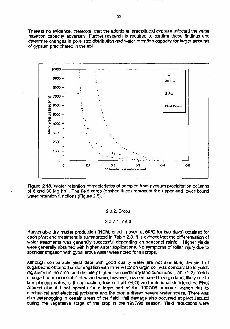
33

There is no evidence, therefore, that the additional precipitated gypsum affected the waterretention capacity adversely. Further research is required to confirm these findings anddetermine changes in pore size distribution and water retention capacity for larger amountsof gypsum precipitated in the soil.

c

c pr

essu

re h

ead

(nM

atr

9000 -

8000 -

7000 -

6000 -

5000 -

4000 -

3000 -

2000 -

1000 -

U -i0

1

1

1

1

m \

1

\

1

\

\

\

\

0.1

1

1

\

I

1

\\

\

\

\

\

\

\

* v.

^ . • _ ~ -~- • "~ - .

0.2 0.3Volumetric soil water content

30t/ha

8t/ha

Field Cores

0.4 0.5

Figure 2.18. Water retention characteristics of samples from gypsum precipitation columnsof 8 and 30 Mg ha'1. The field cores (dashed lines) represent the upper and lower boundwater retention functions (Figure 2.8).

2.3.2. Crops

2.3.2.1. Yield

Harvestable dry matter production (HDM, dried in oven at 60°C for two days) obtained foreach pivot and treatment is summarized in Table 2.3. It is evident that the differentiation ofwater treatments was generally successful depending on seasonal rainfall. Higher yieldswere generally obtained with higher water applications. No symptoms of foliar injury due tosprinkler irrigation with gypsiferous water were noted for all crops.

Although comparable yield data with good quality water are not available, the yield ofsugarbeans obtained under irrigation with mine water on virgin soil was comparable to yieldsregistered in the area, and definitely higher than under dry land conditions (Table 2.3). Yieldsof sugarbeans on rehabilitated land were, however, low compared to virgin land, likely due tolate planting dates, soil compaction, low soil pH (H2O) and nutritional deficiencies. PivotJacuzzi also did not operate for a large part of the 1997/98 summer season due tomechanical and electrical problems and the crop suffered severe water stress. There wasalso waterlogging in certain areas of the field. Hail damage also occurred at pivot Jacuzziduring the vegetative stage of the crop in the 1997/98 season. Yield reductions were

34

experienced due to waterlogging at pivot Tweefontein. The yield of sugarbeans onrehabilitated land was not better in the 1998/99 summer season compared to 1997/98, evenafter levelling works were carried out and waterways built to prevent waterlogging in certainareas of the field. Sugarbeans were, therefore, replaced by maize during the 1999/00season.

Particular attention is therefore required in managing irrigations on rehabilitated soil profileson top of a spoil profile. The hydraulic conductivity of the spoil layer is generally at least oneorder of magnitude lower than that of the overlying soil (Lorentz et al., 1999). This canprevent free percolation of water and leaching of salts, and has significant ramifications withrespect to waterlogging and the lateral flow process. Ponding occurred during the rainysummer season, probably due to subsurface drainage from higher areas. A spatial variabilitystudy and a two-dimensional model are recommended to accurately predict crop growth andwater use, as well as the water and salt balance under such conditions. In the rehabilitationprocess, the spoil material should be packed on a slight slope to minimize lateral flowaccumulation, if rehabilitated land is to be used for crop production under irrigation. Spoilslumping over time is likely to remain problematic.

Excellent yields of wheat were obtained on both virgin and rehabilitated land (Table 2.3).Wheat is reportedly more tolerant to soil salinity than beans (Maas, 1986). The yield of theshort-season cultivar of maize was also good on virgin land (1998/99 season).

The maize crops were damaged in the beginning of the 1999/00 season, when an excess ofherbicide (up to 3 times the planned rate) was mistakenly applied to all three pivots by thefarming company. This resulted in yield losses (Table 2.3). The expected yields werebetween 6 and 10 Mg ha"1 for the short-season cultivar. It was therefore decided toinvestigate the effect of mine water on herbicide activity. The results are presented inSection 2.4.2. of this report. The high rainfall experienced during the cropping season alsoaffected the crops by causing some waterlogging and flooding in the pivot areas. This wasparticularly evident at Tweefontein pivot (rehabilitated ground), but also occurred at pivotMajor. This resulted in areas of poor yield and localized flooding with associated crop death.The maize hybrid used in the short cropping season was chosen for the BT-gene, which issupposed to limit insect damage. However, it appears that this hybrid is very susceptible toNorthern Leaf Blight (rust). This proved to be the case and extensive rust was noted on thecrops near the end of the season. A neighbouring farmer planted the same hybrid early inthe season, which served as a source of infection for the pivots with the Northern Leaf Blight.This was also a reason for the reduced yield obtained. Fungicide applications were requiredto control the spread of the Northern Leaf Blight within the pivots.

In October 2000, a hail storm completely wiped out the wheat crops at pivots Fourth andTweefontein. The estimated loss in crop at pivot Major was 40%. The hail storm occurredduring the grain filling stage of wheat. The potential yield at all three pivots was 8 Mg ha'1.

In conclusion, commercial production of crops under irrigation with gypsiferous mine water isfeasible. Higher yields can be achieved with higher mine water applications, in particularcompared to dry land cropping. The major problem experienced was waterlogging in certainareas of rehabilitated land, especially during the summer months, when control over the soilwater regime is difficult due to rainfall. This problem is related to the physical nature ofrehabilitated land, where levelling of the spoil material and overlying soil is essential due tothe low hydraulic conductivity of the spoil layer. The problem is not related to the chemistryof the water used for irrigation.

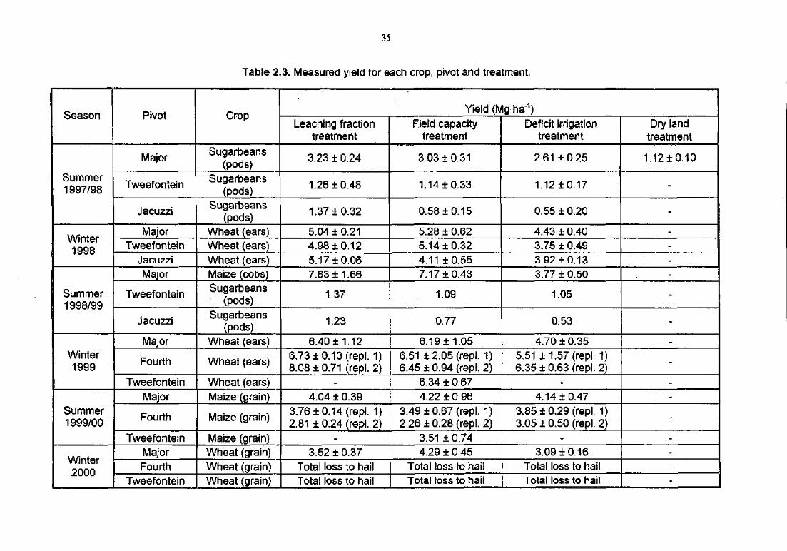
35

Table 2.3. Measured yield for each crop, pivot and treatment.

Season

Summer1997/98

Winter1998

Summer1998/99

Winter1999

Summer1999/00

Winter2000

Pivot

Major

Tweefontein

Jacuzzi

MajorTweefontein

JacuzziMajor

Tweefontein

Jacuzzi

Major

Fourth

TweefonteinMajor

Fourth

TweefonteinMajorFourth

Tweefontein

Crop

Sugarbeans(pods)

Sugarbeans(pods)

Sugarbeans(pods)

Wheat (ears)Wheat (ears)Wheat (ears)Maize (cobs)Sugarbeans

(pods)Sugarbeans

(pods)Wheat (ears)

Wheat (ears)

Wheat (ears)Maize (grain)

Maize (grain)

Maize (grain)Wheat (grain)Wheat (grain)Wheat (grain)

Yield (Mg ha"1)Leaching fraction

treatment

3.23 ± 0.24

1.26 ±0.48

1.37 + 0.32

5.04 ± 0.214.98 ±0.125.17 ±0.067.83 ±1.66

1.37

1.23

6.40 ±1.126.73 ±0.13 (repl. 1)8.08 ± 0.71 (repl. 2)

-

4.04 ±0.393.76 ±0.14 (repl. 1)2.81 ± 0.24 (repl. 2)

-3.52 ± 0.37

Total loss to hailTotal loss to hail

Field capacitytreatment

3.03 ±0.31

1.14 ±0.33

0.58 ±0.15

5.28 ± 0.625.14 ±0.324.11 ±0.557.17 ±0.43

1.09

0.77

6.19 ±1.056.51 ± 2.05 (repl. 1)6.45 ± 0.94 (repl. 2)

6.34 ± 0.674.22 ± 0.96

3.49 ± 0.67 (repl. 1)2.26 ±0.28 (repl. 2)

3.51 ± 0.744.29 ± 0.45

Total loss to hailTotal loss to hail

Deficit irrigationtreatment

2.61 ± 0.25

1.12 ±0.17

0.55 ± 0.20

4.43 ± 0.403.75 ± 0.493.92 ±0.133.77 ±0.50

1.05

0.53

4.70 ±0.355.51 ±1.57 (repl. 1)6.35 ± 0.63 (repl. 2)

-4.14 ±0.47

3.85 ± 0.29 (repl. 1)3.05 ± 0.50 (repl. 2)

-3.09 ±0.16

Total loss to hailTotal loss to hail

Dry landtreatment

1.12±0.10

-

-

---

-

-

-

-

--

-

----

36

2.3.2.2. Plant nutrition

Chemical analyses of plant material were carried out in order to indicate possible nutrientdeficiencies during the growth of the crops, and correct these deficiencies throughfertilization. This was done on wheat, lucerne, sugarbeans and maize. The complete resultsof analyses of plant material are presented in Tables A9 to A15 (Appendix A). In thesetables, normal ranges for each analysis are also reported.

In 1998, the N contents of wheat were normal at the early stage. They became fairly high 70to 80 days after planting and were normal again towards the end of the growing season. Kcontents on most samples were on the lower end of the normal range and were low towardsthe end of the growing season on pivots Jacuzzi and Major. The remaining analyses ofwheat plant material were normal. In September 1998, the P contents of lucerne were lowand the K contents were very low. The remaining analyses were normal.

In February 1999, the plant analysis values for sugarbeans were generally normal. Stuntedgrowth was, however, observed at pivot Jacuzzi and this could be due too a low P content.Chlorotic symptoms were also observed at pivot Jacuzzi and could be due to low N content.This can be possibly due to the poor drainage at pivot Jacuzzi.

In 2000, the N and P contents during the early growth stages (tillering) of wheat were low atpivot Major. At later stages, these values were in the adequate range. The K content washigher than normal throughout the different growth stages. S was also higher than normal.The remaining analyses were normal.

At pivot Tweefontein, N was low during the tillering stage of wheat (winter 2000 season), butbecame normal to high at the latter growth stages. K and S were higher than normal. Thecontents of Fe, Mn and Zn were higher than normal and this could be due to wet conditionscaused by periodic waterlogging.

At pivot Fourth, the N contents of wheat (winter 2000 season) were on the low sidethroughout the growing season. K was high and became very high towards the later stagesof the growing season. S was also high. The remaining analyses were normal.

In conclusion, specific fertilization and monitoring of the nutrient status of the crop is requiredunder irrigation with gypsiferous mine water. Waterlogging should be avoided because of thenegative effect not only on the plants due to high concentrations of SCU and Ca as well asFe, Mn and Zn in the soil solution, but also on gypsum precipitation. Further, the possibilitythat other sulphate minerals can precipitate (or might have) must be investigated.

2.3.3. Soils

2.3.3.1. Chemical properties

In this Section of the report, the general trends of soil chemical properties are reported ingraphical format based on chemical analyses carried out at regular intervals on soil samplescollected in the field. The complete results of soil chemical analyses are reported inAppendix A (Tables A16 to A39 in chronological order). Due to dry soil profiles, it wasgenerally not possible to extract enough soil water with the ceramic cups for chemicalanalysis at the deficit strategy intensive monitoring stations. For this reason, soil sampleswere taken in the deficit treatments on 19/10/1998 for analysis (Table A25, Appendix A). InTables A16 to A39 (Appendix A), the cation exchange capacity was calculated as the sum ofexchangeable Ca2+, K+, Mg2+ and Na+. The charge balances are also reported in the rightcolumn of each Table. The positive sign of the charge balance indicates excess of cations.

37

These differences could be due to the presence of other ions in solution that were notanalysed.

The values of soil pH(H2O) generally showed a slight tendency to increase during the courseof the trial at all pivots (Figures 2.19 to 2.22). The electrical conductivity and the soluble tonsin the saturated soil extract fluctuated depending on seasonal rainfall as well as on theirrigation and rainfall events prior to soil sampling. They did not, however, reach levelsdeleterious to the plants as the main ions in the soil solution precipitated in the form ofCaSO4 and due to the dilution effect of rainfall. The general tendencies are shown in theexamples in Figures 2.23 to 2.37 for pivot Major, which was irrigated throughout the durationof the field trial. The electrical conductivity and soluble Ca2+, Mg2+ and SO42" generallyshowed a tendency to increase with time at ail four pivot sites, due to the relatively highconcentrations of these ions in irrigation water. The values of soluble K+ did not show anyparticular trend and they were lower by one order of magnitude than the other cations(Figures 2.32 to 2.34), as the irrigation water has a low K+ concentration.

Exchangeable Ca2t and Mg2+ increased with time, whilst K+ decreased at all four pivot sites.Examples are shown for exchangeable Ca2+ and K+ at pivot Major (Figures 2.38 to 2.43).This indicates that Ca2+ and, to a certain extent Mg2+, replace K+ on the cation exchangecomplex. If loss of K+ through leaching causes nutrient deficiencies to the crop, correctivefertilization should be applied as symptoms appear. Field monitoring of crop nutrient status istherefore essential at this stage of the research. Very low values of exchangeable Na+ weremeasured during the course of the trial. The cation exchange capacity, calculated as thesum of adsorbed Ca2+, Mg2+, Na+ and K+, showed a slight tendency to increase during thecourse of the trial. An example is shown for pivot Major and three irrigation treatments inFigures 2.44 to 2.46.

Deep soil sampling was carried out before the beginning of the winter 2000 season (June2000). This was done in order to explore whether any salt breakthrough originating fromirrigation could be identified deeper in the soil profile. Replicate sub-samples were analysedby both the Department of Geology (University of Cape Town) and the Soil ScienceLaboratory at the University of Pretoria for double-checking purposes. Some of the results ofthe analyses carried out at the University of Pretoria are summarized in Figures 2.47 to 2.58.It is clear that, at pivot Major, most soluble salts were confined to the upper 1 m, probablydue to the presence of the plinthic layer at 1.1 m limiting free drainage. At pivot Fourth, therewas a more uniform distribution of salts in the soil profile, with a slight peak between 1.5 and2 m down in the profile indicating leaching of salts below the root-zone. The deep soilsampling at pivot Tweefontein included a sample in the spoil material (deepest data points inFigures 2.49, 2.52, 2.55 and 2.58). The detailed analysis results obtained at the University ofPretoria, can be found in Tables A34 to A36 (Appendix A). The detailed analyses of deepsoil samples carried out at the University of Cape Town are presented in Appendix I. Similartrends in the results of the analyses were observed in both laboratories.

Chemical analyses of soil water extracted with ceramic cup soil water samplers are shown inTables A40 to A49 (Appendix A). The results of the analyses confirmed that soil salinity is avery dynamic property as it depends on many factors, mainly rainfall, irrigation amounts andquality, and evapotranspiration. The data generally indicated higher soil salinity in the topsoillayers (ceramic cups placed at 0.4 m soil depth) compared to deeper layers (ceramic cupsplaced at 1.0 and 1.4 m soil depth). This proves that salt, in particular gypsum, accumulatesand precipitates where the rooting system is most dense. During the 1999/00 summerseason, high salinity was recorded at pivot Fourth at 1.0 m, particularly in the deficit irrigationtreatment (Table A48, Appendix A). This was due to salt leaching caused by heavy rainfall.

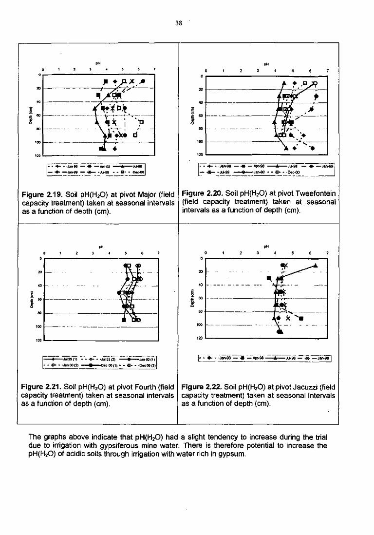
38

PH

- - JaitOS — -m- — Apr-es * Ji>8SI— •• • —Jan-99 — • * — -Js*-S9 - - a - - -DM.00

Figure 2.19. Soil pH(H2O) at pivot Major (fieldcapacity treatment) taken at seasonal intervalsas a function of depth (cm).

• •*• - -Jaiv9S — •

• -X Jli-99

-Apr-98 * Jii-93 —

'-Jan-OO - - O - - -Dec-00

Figure 2.20. Soil pH(H2O) at pivot Tweefontein(field capacity treatment) taken at seasonalintervals as a function of depth (cm).

- - O- - -Jan00(2)- •Jii99(2) — • Jan 00(1)

Dec 00(11 - - D- - •Dec»(2|

. - -Jan-93 — « — Apf-98 - -Jtf-98 — -X- — Jan-99

Figure 2.21. Soil pH(H2O) at pivot Fourth (fieldcapacity treatment) taken at seasonal intervalsas a function of depth (cm).

Figure 2.22. Soil pH(H2O) at pivot Jacuzzi (fieldcapacity treatment) taken at seasonal intervalsas a function of depth (cm).

The graphs above indicate that pH(H2O) had a slight tendency to increase during the trialdue to irrigation with gypsiferous mine water. There is therefore potential to increase thepH(H2O) of acidic soils through irrigation with water rich in gypsum.

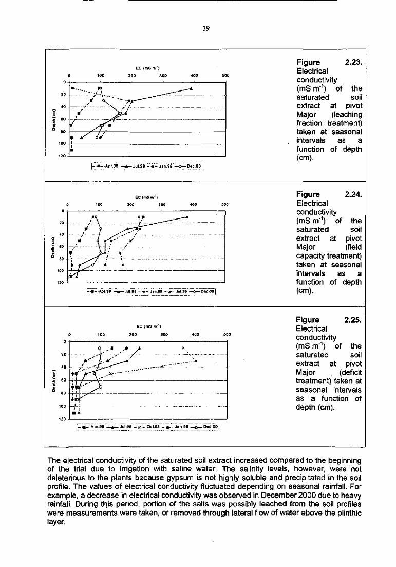
39

EC (mS m'1)

200 300 400 600

100

- •—•Apr .98 Jul,98 - • • - Jan.99 -Dec,00

Figure 2.23.Electricalconductivity(mS m"1) of thesaturated soilextract at pivotMajor (leachingfraction treatment)taken at seasonalintervals as afunction of depth(cm).

EC(mSm' l

200 300

- • - . A p r . 9 8 —*—Jul.96 - • • - Jtn.99 - • * - • Jur.99 —O— Dec.00

Figure 2.24.Electricalconductivity<mS m"1) of thesaturated soilextract at pivotMajor (fieldcapacity treatment)taken at seasonalintervals as afunction of depth(cm).

Figure 2.25.Electricalconductivity(mS m"1) of thesaturated soilextract at pivotMajor . (deficittreatment) taken atseasonal intervalsas a function ofdepth (cm).

The electrical conductivity of the saturated soil extract increased compared to the beginningof the trial due to irrigation with saline water. The salinity levels, however, were notdeleterious to the plants because gypsum is not highly soluble and precipitated in the soilprofile. The values of electrical conductivity fluctuated depending on seasonal rainfall. Forexample, a decrease in electrical conductivity was observed in December 2000 due to heavyrainfall. During this period, portion of the salts was possibly leached from the soil profileswere measurements were taken, or removed through lateral flow of water above the plinthiclayer.

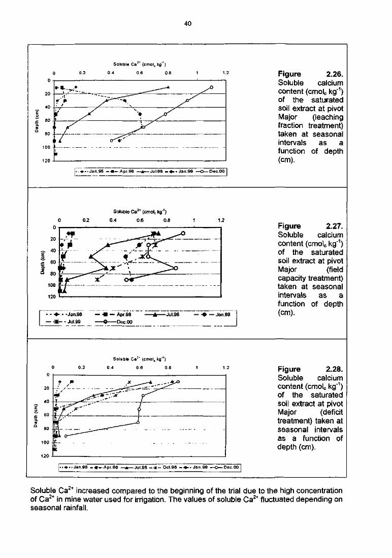
40

0.2

Soluble Ca2' (cmolc kg'1)

0.4 0.6 0.8 1.2

120

. ••.Jan.98 -••-•Apr.98 —4—Jul.SB - « - - Jan.99 -Dec.00

Figure 2.26.Soluble calciumcontent (cmolc kg"1)of the saturatedsoil extract at pivotMajor (leachingfraction treatment)taken at seasonalintervals as afunction of depth(cm).

0.2

Soluble Ca2* (cmolc kg"1)

0.4 0.6 0.8

•Jan.98 —

• Jul.99 —

• Apr .98

-Dec.00

- Jul.98 — ••• — Jan.99

Figure 2.27.Soluble calciumcontent (cmolc kg"1)of the saturatedsoil extract at pivotMajor (fieldcapacity treatment)taken at seasonalintervals as afunction of depth(cm).

0.2

Soluble Ca !' (cmolt kg"1)

0.4 0.6 0.8

• •»... Jan 96 -••-•Apr.QS -Jul.98 - * - Oct.9S - • - • Jan.99 -Dec.00

Figure 2.28.Soluble calciumcontent (cmolo kg"1)of the saturatedsoil extract at pivotMajor (deficittreatment) taken atseasonal intervalsas a function ofdepth (cm).

Soluble Ca2+ increased compared to the beginning of the trial due to the high concentrationof Ca2+ in mine water used for irrigation. The values of soluble Ca2+ fluctuated depending onseasonal rainfall.

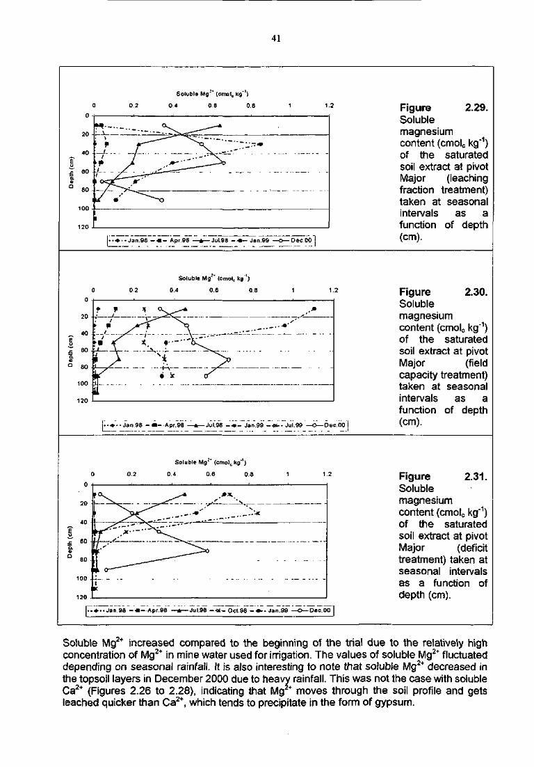
41

0.2

Soluble Mg 3 ' (cmol t Kg"1)

0.4 0.6 O.B 1.2

100

120

[ • • • • • J a n . 9 8 - * - Apr.98 — * — J u l . 9 8 - * - Jan.99 —O—Dec.00 j

Figure 2.29.Solublemagnesiumcontent (cmolc kg"1)of the saturatedsoil extract at pivotMajor (leachingfraction treatment)taken at seasonalintervals as afunction of depth(cm).

0,2

Soluble Mg (cmolt kg')

0.4 0.6 OB 1.2

• • • • Jan 98 - a- .Apr .96 —A—Jul.98 — • • - Jan.99 — -as-- Jul.99 —o—Dec.00

Figure 2.30.Solublemagnesiumcontent (cmol0 kg"1)of the saturatedsoil extract at pivotMajor (fieldcapacity treatment)taken at seasonalintervals as afunction of depth(cm).

0.2

Soluble Mg2* (cmolc kg"')

0.4 0.8 0.8 1.2

120

[^• • •Jan.98 - • - • A p r . 9 8 —*—Jul.98 - • * - Oct.96 - • - • Jan.99 —o— Dec

Figure 2.31.Solublemagnesiumcontent (cmolc kg"1)of the saturatedsoil extract at pivotMajor (deficittreatment) taken atseasonal intervalsas a function ofdepth (cm).

Soluble Mg2+ increased compared to the beginning of the trial due to the relatively highconcentration of Mg2+ in mine water used for irrigation. The values of soluble Mg2+ fluctuateddepending on seasonal rainfall. It is also interesting to note that soluble Mg2+ decreased inthe topsoil layers in December 2000 due to heavy rainfall. This was not the case with solubleCa2+ (Figures 2.26 to 2.28), indicating that Mg moves through the soil profile and getsleached quicker than Ca2+, which tends to precipitate in the form of gypsum.

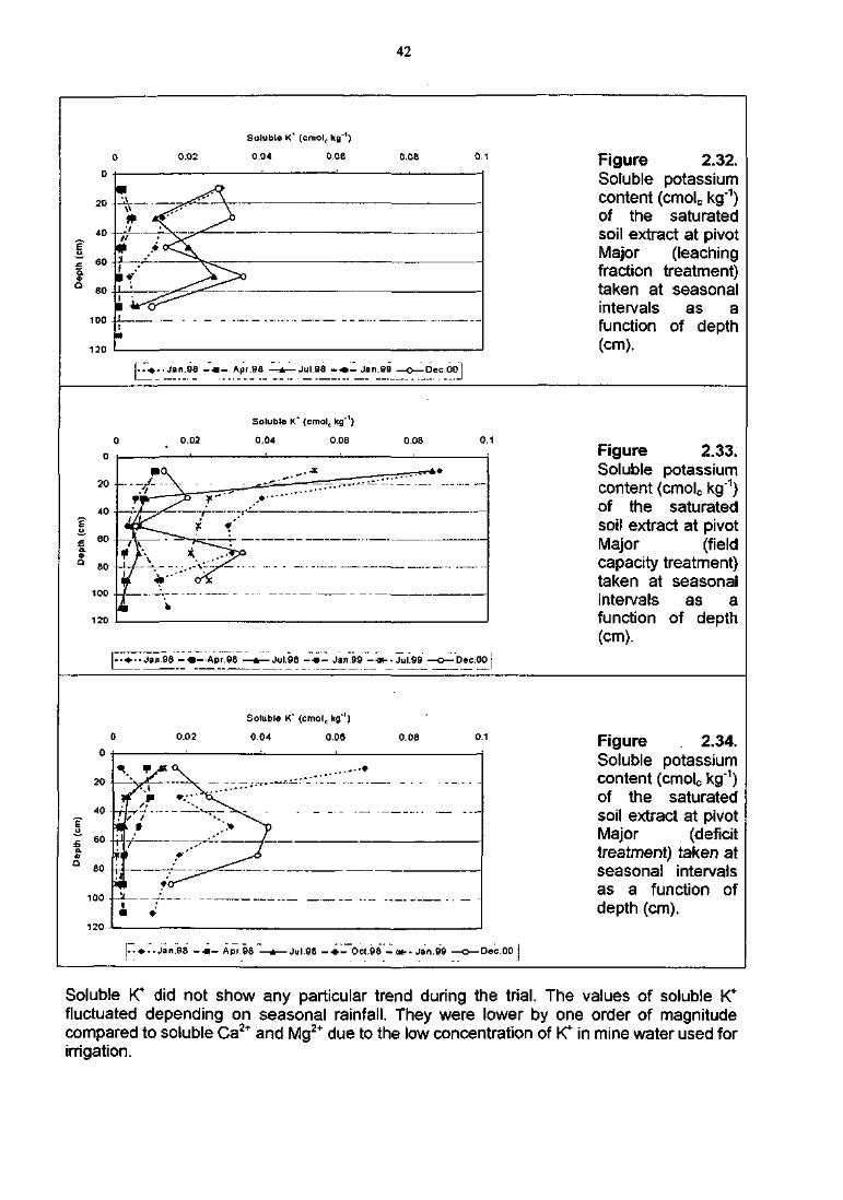
42

0.02

Soluble K (cmolc kg'1)

0,04 0 06 o.oa 0.1

80

1 oo -i

120

• •••Jan.98 - • • - Apr.98 - Jul.98 - « - Jan.99 -Dec.00

Figure 2.32.Soluble potassiumcontent (cmolc kg'1)of the saturatedsoil extract at pivotMajor (leachingfraction treatment)taken at seasonalintervals as afunction of depth(cm).

0.02

Soluble K (cmolc kg )

0.04 0.06 0.08 0.1

- . • • • Jan.98 - • - • A p r . 9 8 —*—Jul.9B - • • - Jan.99 - • * - . Jul.99 —o—Dec.OOt

Figure 2.33.Soluble potassiumcontent (cmolc kg"1)of the saturatedsoil extract at pivotMajor (fieldcapacity treatment)taken at seasonalintervals as afunction of depth(cm).

0.02

Soluble K* (cmole kg'1)

0.04 0.06 0.08

P".».. Jan.98 -•m- Apr.98 —*—Jul.9B - * - Oct.98 - « - . Jan.99 —o—Dec.00

Figure 2.34.Soluble potassiumcontent (cmolc kg"1)of the saturatedsoil extract at pivotMajor (deficittreatment) taken atseasonal intervalsas a function ofdepth (cm).

Soluble IC did not show any particular trend during the trial. The values of soluble K+

fluctuated depending on seasonal rainfall. They were lower by one order of magnitudecompared to soluble Ca2+ and Mg2+ due to the low concentration of K+ in mine water used forirrigation.

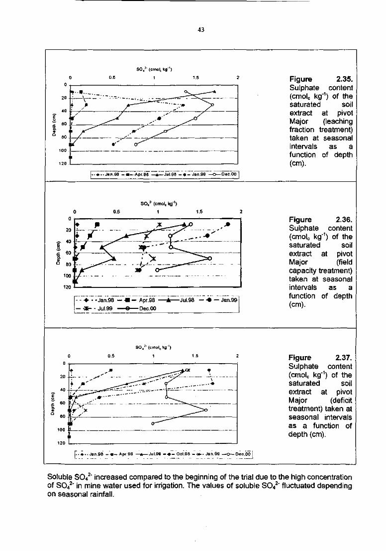
43

vD

80 . _ y l

100

120

; - . * . . Jan.93 - « - . A p r . 9 6 —*—JuL98 - • - Jan.99 —O—Dec.Ool

Figure 2.35.Sulphate content(cmolc kg'1) of thesaturated soilextract at pivotMajor (leachingfraction treatment)taken at seasonalintervals as afunction of depth(cm).

SO42' (cmolt kg"1)

1 1.5

••• - -Jan.98 — •

- -3K- -JUI .99 —

Apr.98 •

-Dec.00

-Jut.98 — • • — Jan.99

Figure 2.36.Sulphate content(cmolc kg'1) of thesaturated soilextract at pivotMajor (fieldcapacity treatment)taken at seasonalintervals as afunction of depth(cm).

120

[^••••Jan.98 - * - A p r , 9 8 —* lul.96 - • • - Oct.98 - « - . Jan.99 —o— Dec.00 j

Figure 2.37.Sulphate content(cmolc kg'1) of thesaturated soilextract at pivotMajor (deficittreatment) taken atseasonal intervalsas a function ofdepth (cm).

Soluble SO4 increased compared to the beginning of the trial due to the high concentrationof SO4

2' in mine water used for irrigation. The values of soluble SCu2' fluctuated dependingon seasonal rainfall.

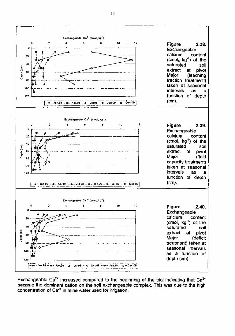
44

Exchangeable Ca3 '(cmol£ kg 1)

10 12

120

I-. •-•Jan.98 - • - Apr.98 —*—Jul.98 - « - JJul.98 - « - Jan.99 —o—Oec.00

Figure 2.38.Exchangeablecalcium content(cmolc kg'1) of thesaturated soilextract at pivotMajor (leachingfraction treatment)taken at seasonalintervals as afunction of depth(cm).

Exchangeable Ca (cmol, kg )

4 6 6

L. «... Jan.98 - • - • A p r , 98 —*—Jul.98 - - » - Jan.99 - • * - - Jul 99 —c—Oec.00 I

Figure 2.39.Exchangeablecalcium content(cmolc kg"1) of thesaturated soilextract at pivotMajor (fieldcapacity treatment)taken at seasonalintervals as afunction of depth(cm).

Exchangeable Ca2 ' (cmolc kg'1)

4 6 6 10 12

120

- • • -Jan.98 — * - Apr.98 -Jul.98 - - » - O c t 9 8 - • - • Jan.99 -Dee.00

Figure 2.40.Exchangeablecalcium content(cmolc kg'1) of thesaturated soilextract at pivotMajor (deficittreatment) taken atseasonal intervalsas a function ofdepth (cm).

Exchangeable Ca2+ increased compared to the beginning of the trial indicating that Ca2+

became the dominant cation on the soil exchangeable complex. This was due to the highconcentration of Ca2+ in mine water used for irrigation.

45

0.1

Exchangeable K* (cmolc

0.2 0.3 0.1 0.5 0.6 0-7

20

40 ^ v A 1

120

•ATrk

** • ' • ' . .

>

* >

60 .—,

ao —:.

100

! - • • • • Jan.98 - • - Apr.98 -Jul.98 - « - Jan.99 -Dec.00

Figure 2.41.Exchangeablepotassiumcontent (cmolckg"1) of thesaturated soilextract at pivotMajor (leachingfractiontreatment) takenat seasonalintervals as afunction of depth(cm).

0 1

Exchangeable K* (cmolc kg'1)

0.2 0,3 0.4 0.5 0.6

- • • - - Jan.96 - • — Apt.96 —*—Jul.98 - •— Jan.99 - < * • • Jul.99 —O—Dec.00 !

Figure 2.42.Exchangeablepotassiumcontent (cmolckg"1) of thesaturated soilextract at pivotMajor (fieldcapacitytreatment) takenat seasonalintervals as afunction of depth(cm).

0.1

Exchangeable K* (cmol, kg'1)

0.2 0.3 0.4 0.5 0.6 0.7

an.98 - • - Apt.98 -Jul.98 -.sue- QctSS - • • Jan.99 - Dec.QO

Figure 2.43.Exchangeablepotassiumcontent (cmolckg"1) of thesaturated soilextract at pivotMajor (deficittreatment) takenat seasonalintervals as afunction of depth(cm).

Exchangeable K+ decreased compared to the beginning of the trial indicating that K+ wasdisplaced, mainly by Ca2+, on the soil exchangeable complex. This was due to the highconcentration of Ca2+ and low concentration of fC in mine water used for irrigation. As K+ isnot retained by the soil adsorptive complex, there is a potential risk of K+ leaching and thenutrient status of the plants should be monitored and corrected through fertilization.

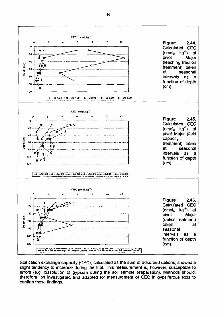
46

CEC

10 12

120

[*-••-• Jan. 98 - • • - Apr.98 —*—Jul.QB - « - Jan.99 —o—Dee.DO I

Figure 2.44.Calculated CEC(cmolG kg"1) atpivot Major(leaching fractiontreatment) takenat seasonalintervals as afunction of depth(cm).

CEC

10 12

.Jan.98 - • - -Jul.98 - • - Jan.99 - • * • • JuJ.99 -Dec.00

Figure 2.45.Calculated CEC(cmolc kg'1) atpivot Major (fieldcapacitytreatment) takenat seasonalintervals as afunction of depth(cm).

CEC (cmol.kg1)

4 6 8 12

120

• •..Jaiv98 -«-~AprS5 —*—Jui.98~-« - Oct.98 - • - • Jan.99 —O— bec.OO |

Figure 2.46.Calculated CEC(cmolc kg"1) atpivot Major(deficit treatment)taken atseasonalintervals as afunction of depth(cm).

Soil cation exchange capacity (CEC), calculated as the sum of adsorbed cations, showed aslight tendency to increase during the trial. This measurement is, however, susceptible toerrors (e.g. dissolution of gypsum during the soil sample preparation). Methods should,therefore, be investigated and adapted for measurement of CEC in gypsiferous soils toconfirm these findings.

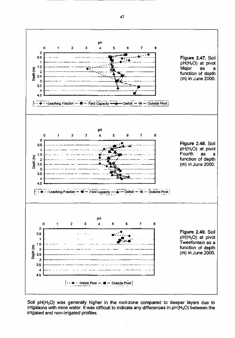
47

[ - - • » • ' • - Leaching Fraction — - • — Field Capacity — + — D e f i c i t — -X — Outside Pivot

Figure 2.47. SoilpH(H2O) at pivotMajor as afunction of depth(m) in June 2000.

f- • • - -Leaching Fraction — - • — Field Capacity • • Deficit — -X — Outside Pivot

Figure 2.48. SoilpH(H2O) at pivotFourth as afunction of depth(m) in June 2000.

(0

0.5

1

„ 1.5 •

3-2.5-° 3

3.5 •

4ACL .

) 1

_ . ..

2

pH

3 4 5 6 7 S

, •

:.... :_v_._£*i._:.__

• - - Inside Pivot — • — Outside Pivot!

Figure 2.49. SoilpH(H2O) at pivotTweefontein as afunction of depth(m) in June 2000.

Soil pH(H2O) was generally higher in the root-zone compared to deeper layers due toirrigations with mine water. It was difficult to indicate any differences in pH(H2O) between theirrigated and non-irrigated profiles.

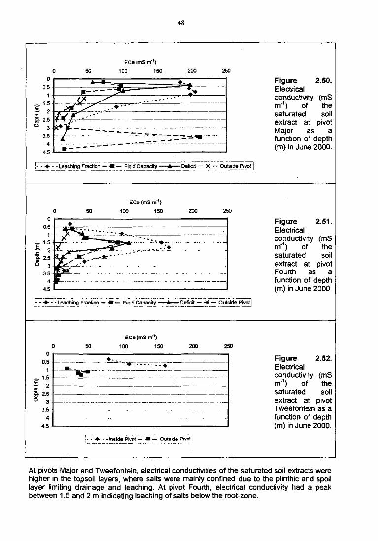
48

50

ECe (mS m'1)

100 150 200 250

- -Leaching Fraction — - • — Field Capacity —•—Def ic i t — -X — Outside Pivot]

FigureElectricalconductivityrrT1) ofsaturatedextract atMajor as

2.50.

(mSthesoil

pivota

function of depth(m) in June 2000.

50

ECe (mS m"1)

100 150 200 250

• - - Leaching Fraction — • • — Field Capacity • - Deficit — -X — Outside Pivot

Figure 2.51.Electricalconductivity <mSm'1) of thesaturated soilextract at pivotFourth as afunction of depth(m) in June 2000.

50

ECe (mS m'1)

100 150 200

; - • • • • - - inside Pivot — - • — Outside Pivot ,t

Figure 2.52.Electricalconductivity (mSrrf1) of thesaturated soilextract at pivotTweefontein as afunction of depth(m) in June 2000.

At pivots Major and Tweefontein, electrical conductivities of the saturated soil extracts werehigher in the topsoil layers, where salts were mainly confined due to the plinthic and spoillayer limiting drainage and leaching. At pivot Fourth, electrical conductivity had a peakbetween 1.5 and 2 m indicating leaching of salts below the root-zone.

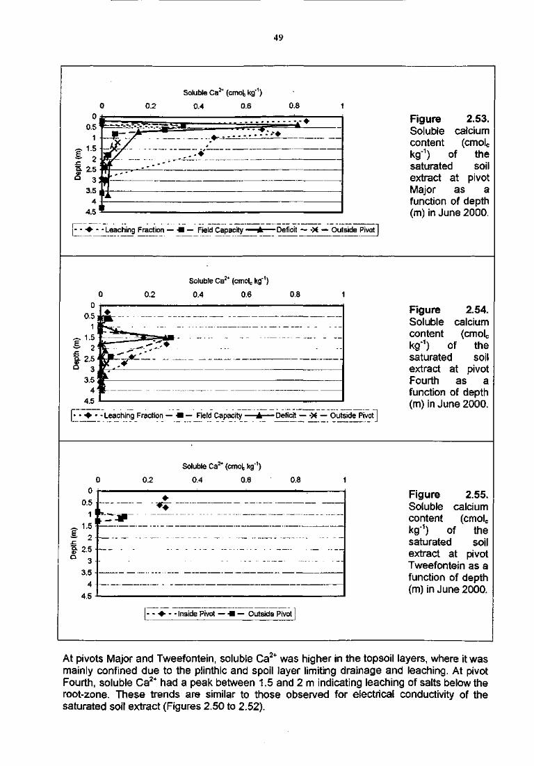
49

Soluble Ca2* (cmot kg"1)

00 j

0.5 J-

A3.5 1

,1*

0.2

j - - ' ' ' '

f

0.4

• L ^ _

#

0.6 0.8 1

[^j • - - Leaching Fraction — • • — Field Capacity — A — Deficit — -X — Outside Pivot j

Figure 2.53.Soluble calciumcontent (cmolckg"1) of thesaturated soilextract at pivotMajor as afunction of depth(m) in June 2000.

Soluble Ca2* (cmolc kg"1)

0.4 0.6 0.8

[•-•••-• Leaching Fraction — • • — Fiefd Capacity — A — Deficit — -X — Outside Pivot

Figure 2.54.Soluble calciumcontent (cmolckg"1) of thesaturated soilextract at pivotFourth as afunction of depth(m) in June 2000.

0.2

Soluble Ca2* (cmot kg"1)

0.4 0.6 0.8

• - -Inside Pivot — - • — Outside Pivot

Figure 2.55.Soluble calciumcontent (cmolckg"1) of thesaturated soilextract at pivotTweefontein as afunction of depth(m) in June 2000.

At pivots Major and Tweefontein, soluble Ca2+ was higher in the topsoil layers, where it wasmainly confined due to the piinthic and spoil layer limiting drainage and leaching. At pivotFourth, soluble Ca2+ had a peak between 1.5 and 2 m indicating leaching of salts below theroot-zone. These trends are similar to those observed for electrical conductivity of thesaturated soil extract (Figures 2.50 to 2.52).

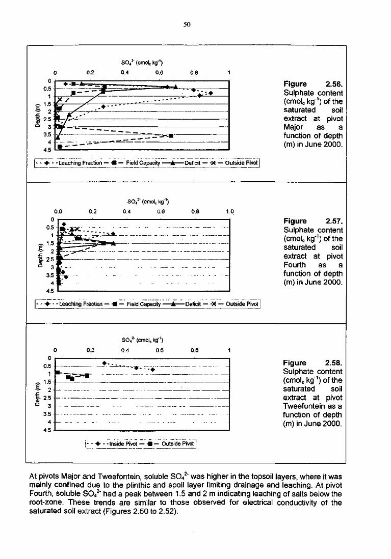
50

0.2

SO42" (cmole kg"1)

0.4 0.6

f- - • • -Leaching Fraction — • • — Field Capacity — £ — D e f i c i t — -X — Outside Pivot |

Figure 2.56.Sulphate content(cmoic kg"1) of thesaturated soilextract at pivotMajor as afunction of depth(m) in June 2000.

o.o

SO*2" (cmolc kg"1)

0.4 0.6 0.8 1.0

- - Leaching Fraction — • • — Field Capacity • -Deficit — -X — Outside Pivot

Figure 2.57.Sulphate content(cmolc kg"1) of thesaturated soilextract at pivotFourth as afunction of depth(m) in June 2000.

0.2

SO42" (cmolc kg'1)

0.4 0.6 0.8

- - Inside Pivot — -U — Outside Pivot

Figure 2.58.Sulphate content(cmolc kg"1) of thesaturated soilextract at pivotTweefontein as afunction of depth(m) in June 2000.

At pivots Major and Tweefontein, soluble SO42' was higher in the topsoil layers, where it was

mainly confined due to the plinthic and spoil layer limiting drainage and leaching. At pivotFourth, soluble S O / ' had a peak between 1.5 and 2 m indicating leaching of salts below theroot-zone. These trends are similar to those observed for electrical conductivity of thesaturated soil extract (Figures 2.50 to 2.52).

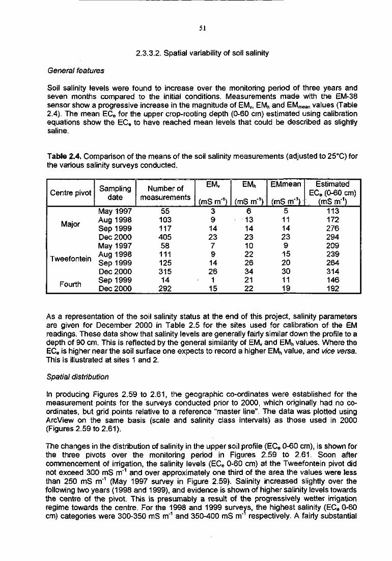
51

2.3.3.2. Spatial variability of soil salinity

General features

Soil salinity levels were found to increase over the monitoring period of three years andseven months compared to the initial conditions. Measurements made with the EM-38sensor show a progressive increase in the magnitude of EMV, EMh and EMmean values (Table2.4). The mean ECe for the upper crop-rooting depth (0-60 cm) estimated using calibrationequations show the ECe to have reached mean levels that could be described as slightlysaline.

Table 2.4. Comparison of the means of the soil salinity measurements (adjusted to 25°C) forthe various salinity surveys conducted.

Centre pivot

•

Major

Tweefontein

ruurtn

Samplingdate

May 1997Aug 1998Sep 1999Dec 2000May 1997Aug 1998Sep 1999Dec 2000Sep 1999Dec 2000

Number ofmeasurements

551031174055811112531514

292

EMV

(mSm-1)3914237914261

15

EMh

(mS rrf1)6131423102226342122

EMmean

(mS m;1)511142391520301119

EstimatedECe (0-60 cm)

: (mS rrf1) :113172276294209239264314146192

As a representation of the soil salinity status at the end of this project, salinity parametersare given for December 2000 in Table 2.5 for the sites used for calibration of the EMreadings. These data show that salinity levels are generally fairly similar down the profile to adepth of 90 cm. This is reflected by the general similarity of EMV and EMh values. Where theECe is higher near the soil surface one expects to record a higher EMh value, and vice versa.This is illustrated at sites 1 and 2.

Spatial distribution

In producing Figures 2.59 to 2.61, the geographic co-ordinates were established for themeasurement points for the surveys conducted prior to 2000, which originally had no co-ordinates, but grid points relative to a reference "master line". The data was plotted usingArcView on the same basis (scale and salinity class intervals) as those used in 2000(Figures 2.59 to 2.61).

The changes in the distribution of salinity in the upper soil profile (ECe 0-60 cm), is shown forthe three pivots over the monitoring period in Figures 2.59 to 2.61. Soon aftercommencement of irrigation, the salinity levels (ECe 0-60 cm) at the Tweefontein pivot didnot exceed 300 mS m"1 and over approximately one third of the area the values were lessthan 250 mS m"1 (May 1997 survey in Figure 2.59). Salinity increased slightly over thefollowing two years (1998 and 1999), and evidence is shown of higher salinity levels towardsthe centre of the pivot. This is presumably a result of the progressively wetter irrigationregime towards the centre. For the 1998 and 1999 surveys, the highest salinity (ECe 0-60cm) categories were 300-350 mS m'1 and 350-400 mS m"1 respectively. A fairly substantial

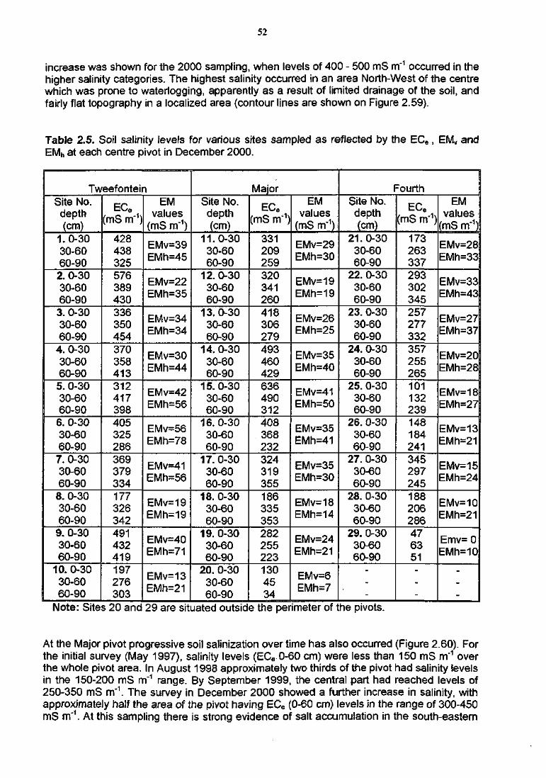
52

increase was shown for the 2000 sampling, when levels of 400 - 500 mS m"1 occurred in thehigher salinity categories. The highest salinity occurred in an area North-West of the centrewhich was prone to waterlogging, apparently as a result of limited drainage of the soil, andfairly flat topography in a localized area (contour lines are shown on Figure 2.59).

Table 2.5. Soil salinity levels for various sites sampled as reflected by the ECe, EMV andEMh at each centre pivot in December 2000.

TweefonteinSite No.depth(cm)

1.0-3030-6060-902. 0-3030-6060-903. 0-3030-6060-90

4. 0-3030-6060-905. 0-3030-6060-90

6. 0-3030-6060-907. 0-3030-6060-908. 0-3030-6060-909. 0-3030-6060-90

10. 0-3030-6060-90

ECe

(mS m"1)

428438325576389430336350454370358413312417398405325286369379334177326342491432419197276303

EMvalues

(mS m"1)

EMv=39EMh=45

EMv=22EMh=35

EMv=34EMh=34

EMv=30EMh=44

EMv=42EMh=56

EMv=56EMh=78

EMv=41EMh=56

EMv=19EMh=19

EMv=40EMh=71

EMv=13EMh=21

MajorSite No.

depth(cm)

11.0-3030-6060-90

12.0-3030-6060-90

13.0-3030-6060-90

14. 0-3030-6060-90

15.0-3030-6060-90

16.0-3030-6060-90

17.0-3030-6060-90

18.0-3030-6060-90

19.0-3030-6060-90

20. 0-3030-6060-90

ECe

(mS nr1)

3312092593203412604183062794934604296364903124083682323243193551863353532822552231304534

EMvalues

(mS rrr1)

EMv=29EMh=30

EMv=19EMh=19

EMv=26EMh=25

EMv=35EMh=40

EMv=41EMh=50

EMv=35EMh=41

EMv=35EMh=30

EMv=18EMh=14

EMv=24EMh=21

EMv=6EMh=7

FourthSite No.depth(cm)

21.0-3030-6060-90

22. 0-3030-6060-90

23. 0-3030-6060-90

24. 0-3030-6060-90

25. 0-3030-6060-90

26. 0-3030-6060-90

27. 0-3030-6060-90

28. 0-3030-6060-90

29. 0-3030-6060-90

-

ECe

(mS m"1)

173263337293302345257277332357255265101132239148184241345297245188206286476351

-

EMvalues

(mS m"1)

EMv=28EMh=33

EMv=33EMh=43

EMv=27EMh=37

EMv=20EMh=28

EMv=18EMh=27

EMv=13EMh=21

EMv=15EMh=24

EMv=10EMh=21

Emv= 0EMh=10

-

Note: Sites 20 and 29 are situated outside the perimeter of the pivots.

At the Major pivot progressive soil salinization over time has also occurred (Figure 2.60). Forthe initial survey (May 1997), salinity levels (ECe 0-60 cm) were less than 150 mS m"1 overthe whole pivot area. In August 1998 approximately two thirds of the pivot had salinity levelsin the 150-200 mS m"1 range. By September 1999, the central part had reached levels of250-350 mS m"1. The survey in December 2000 showed a further increase in salinity, withapproximately half the area of the pivot having ECe (0-60 cm) levels in the range of 300-450mS m~1. At this sampling there is strong evidence of salt accumulation in the south-eastern

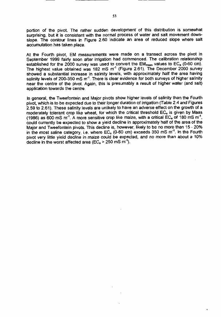
53

portion of the pivot. The rather sudden development of this distribution is somewhatsurprising, but it is consistent with the normal process of water and salt movement down-slope. The contour lines in Figure 2.60 indicate an area of reduced slope where saltaccumulation has taken place.

At the Fourth pivot, EM measurements were made on a transect across the pivot inSeptember 1999 fairly soon after irrigation had commenced. The calibration relationshipestablished for the 2000 survey was used to convert the EMmean values to ECe (0-60 cm).The highest value obtained was 182 mS m'1 (Figure 2.61). The December 2000 surveyshowed a substantial increase in salinity levels, with approximately half the area havingsalinity levels of 200-350 mS rrf1. There is clear evidence for both surveys of higher salinitynear the centre of the pivot. Again, this is presumably a result of higher water (and salt)application towards the centre.

In general, the Tweefontein and Major pivots show higher levels of salinity than the Fourthpivot, which is to be expected due to their longer duration of irrigation (Table 2.4 and Figures2.59 to 2.61). These salinity levels are unlikely to have an adverse effect on the growth of amoderately tolerant crop like wheat, for which the critical threshold ECe is given by Maas(1986) as 600 mS m"1. A more sensitive crop like maize, with a critical ECe of 180 mS m"\could currently be expected to show a yield decline in approximately half of the area of theMajor and Tweefontein pivots. This decline is, however, likely to be no more than 15 - 20%in the most saline category, i.e. where ECe (0-60 cm) exceeds 350 mS m'1. In the Fourthpivot very little yield decline in maize could be expected, and no more than about a 10%decline in the worst affected area (ECB > 250 mS m~1).

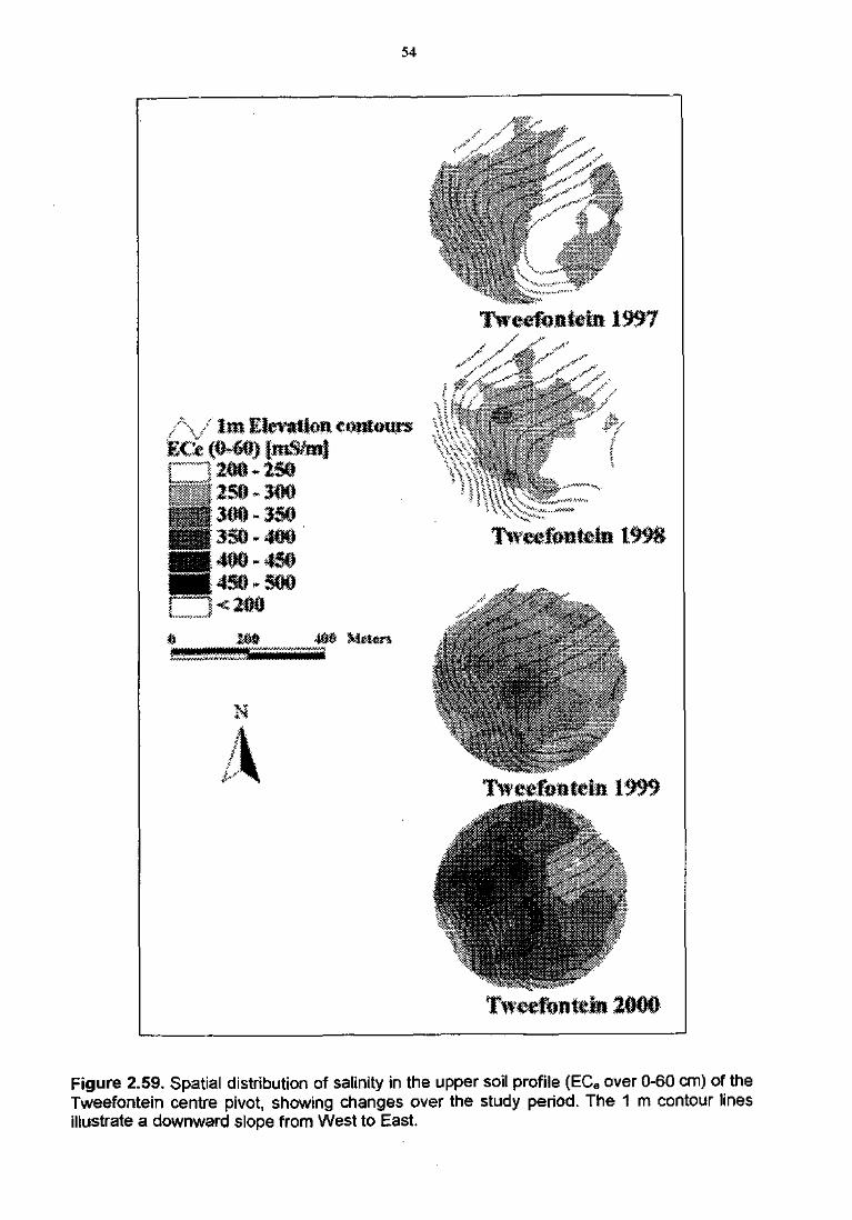
54

A/IJ»Bi

A

in 1997

4 fr - • ' • •

Figure 2.59. Spatial distribution of salinity in the upper soil profile (ECe over 0-60 cm) of theTweefontein centre pivot, showing changes over the study period. The 1 m contour linesillustrate a downward slope from West to East.

55

i

43$-45$1«1S0

" * • • ' . - .

.m

V r ' • • - . T _

. • . • • ' • > • • " ' " ' " - . • • • • • • '

,^.->-'"'"J""

, , , , , v , ^ - - > - V '

" • ^ • • • ^ • - . • ^ • • " ' : ;

, • • • •

Figure 2.60. Spatial distribution of salinity in the upper soil profile (ECe over 0-60 cm) of theMajor centre pivot, showing changes over the study period. The 1 m contour lines illustrate adownward slope from North to South.

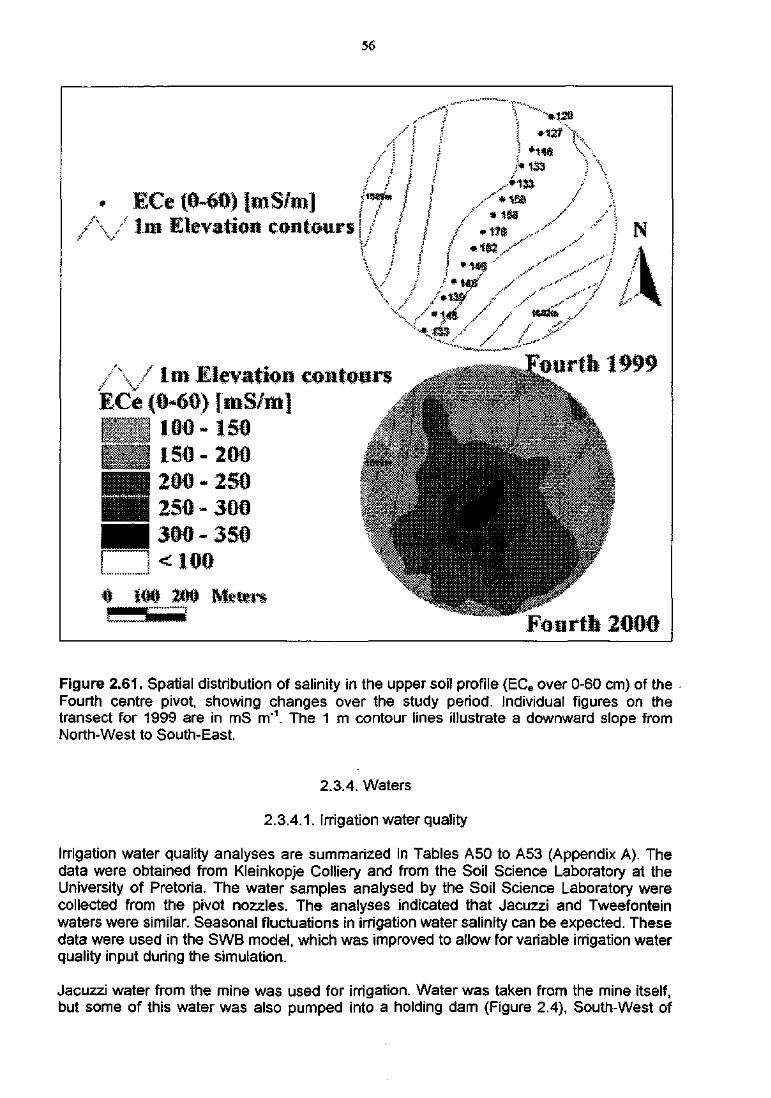
56

A/ \ /

ICe (S-tfO) ImS/m]Elevation

Fotirth

Figure 2.61. Spatial distribution of salinity in the upper soil profile (ECe over 0-60 cm) of theFourth centre pivot, showing changes over the study period. Individual figures on thetransect for 1999 are in mS m*1. The 1 m contour lines illustrate a downward slope fromNorth-West to South-East.

2.3.4. Waters

2.3.4.1. Irrigation water quality

Irrigation water quality analyses are summarized in Tables A50 to A53 (Appendix A). Thedata were obtained from Kleinkopje Colliery and from the Soil Science Laboratory at theUniversity of Pretoria. The water samples analysed by the Soil Science Laboratory werecollected from the pivot nozzles. The analyses indicated that Jacuzzi and Tweefonteinwaters were similar. Seasonal fluctuations in irrigation water salinity can be expected. Thesedata were used in the SWB model, which was improved to allow for variable irrigation waterquality input during the simulation.

Jacuzzi water from the mine was used for irrigation. Water was taken from the mine itself,but some of this water was also pumped into a holding dam (Figure 2.4), South-West of

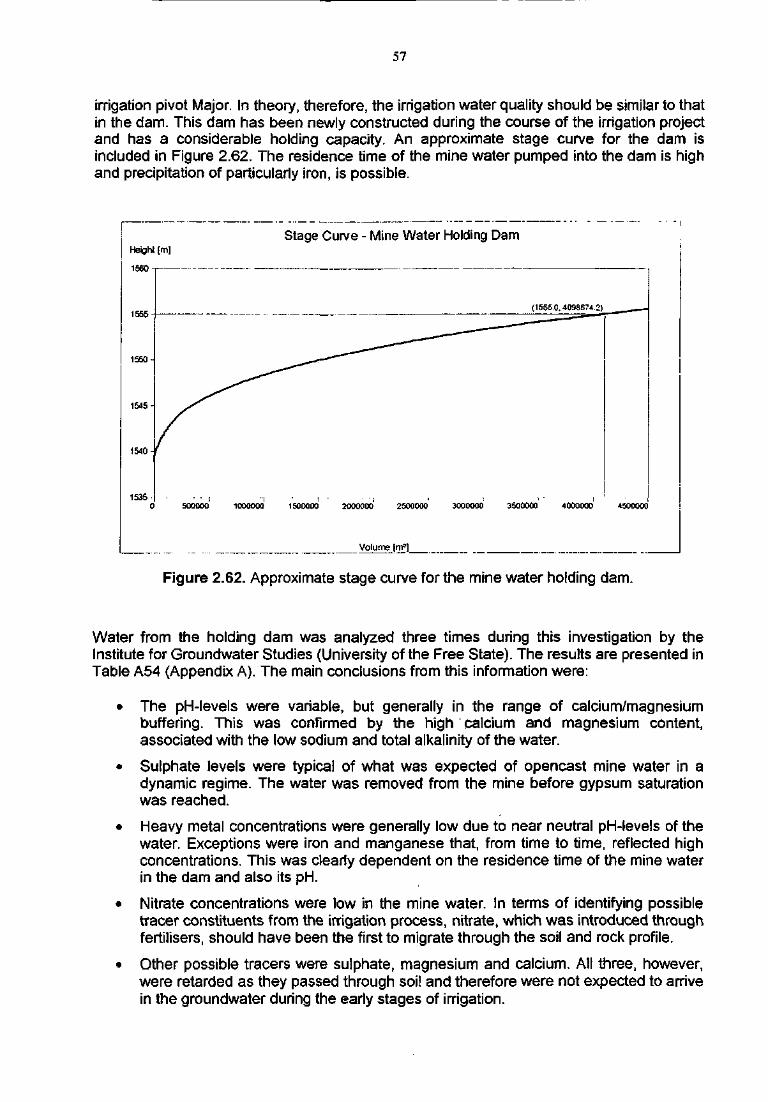
57

irrigation pivot Major. In theory, therefore, the irrigation water quality should be similar to thatin the dam. This dam has been newly constructed during the course of the irrigation projectand has a considerable holding capacity. An approximate stage curve for the dam isincluded in Figure 2.62. The residence time of the mine water pumped into the dam is highand precipitation of particularly iron, is possible.

Stage Curve - Mine Water Holding DamHeigh! [mj

1560 -i

1555

1550-

(1556.0.4098674.2)

0 500000 1000000 150D000 2000000 2500000 3OODO00 3500000 4000DOO 4500000

Volume |rrf]

Figure 2.62. Approximate stage curve for the mine water holding dam.

Water from the holding dam was analyzed three times during this investigation by theInstitute for Groundwater Studies (University of the Free State). The results are presented inTable A54 (Appendix A). The main conclusions from this information were:

• The pH-levels were variable, but generally in the range of calcium/magnesiumbuffering. This was confirmed by the high calcium and magnesium content,associated with the low sodium and total alkalinity of the water.

• Sulphate levels were typical of what was expected of opencast mine water in adynamic regime. The water was removed from the mine before gypsum saturationwas reached.

• Heavy metal concentrations were generally low due to near neutral pH-leve!s of thewater. Exceptions were iron and manganese that, from time to time, reflected highconcentrations. This was clearly dependent on the residence time of the mine waterin the dam and also its pH.

• Nitrate concentrations were low in the mine water. In terms of identifying possibletracer constituents from the irrigation process, nitrate, which was introduced throughfertilisers, should have been the first to migrate through the soil and rock profile.

• Other possible tracers were sulphate, magnesium and calcium. All three, however,were retarded as they passed through soii and therefore were not expected to arrivein the groundwater during the early stages of irrigation.

58

The quality of water in the dam was consistent with the irrigation water qualitiesshown in Tables A50 and A53 (Appendix A).

2.3.4.2. Runoff

From spring 1999, runoff amounts and quality were measured at the weirs at pivot Major andTweefontein. Runoff events and quality of runoff water are summarized in Tables 2.6 (pivotMajor) and 2.7 (pivot Tweefontein). Water flow over the weir (Q) was calculated with thefollowing formula:

Q = 1.585 x 5 x h 2 5

where h is the water level above the weir in m, whilst 1.585, 5 and 2.5 are coefficientsdepending on the shape and size of the weir and used to express flow in m3 s"1. Eachreading of h recorded with the pressure transducer and the data logger, was used tocalculate Q. This was then multiplied by 120 s (reading interval) and summed in order tocalculate the total amount of runoff.

The amount of salts in runoff was calculated using the following equation:

TDS= 10 EC

where TDS is total dissolved salts in g m"3 and EC is the electrical conductivity measuredwith the salinity sensor in mS m'1. The factor "10" is commonly used in the conversion forwaters rich in SO4

2". Each reading of EC recorded with the salinity sensor and the datalogger was used to determine TDS. This was then multiplied by the amount of water in m3

flowing over the weir in 120 s (reading interval) and summed in order to calculate the amountof salts leaving the field in a runoff event. The average EC values in Tables 2.6 and 2.7 areweighted by the water flow during each measurement interval.

The results indicated that less than 2% of the salts added since the beginning of the trial(Tables 3.5 and 3.6) were lost from the irrigated fields through surface and subsurface runofffrom November 1999 until April 2000. More runoff was recorded at pivot Tweefonteincompared to pivot Major, due to the restricted soil depth of the rehabilitated land. Due toimpervious soil layers at pivots Major and Tweefontein, it is likely that runoff and salts inrunoff could have mainly originated from lateral movement of soil water.

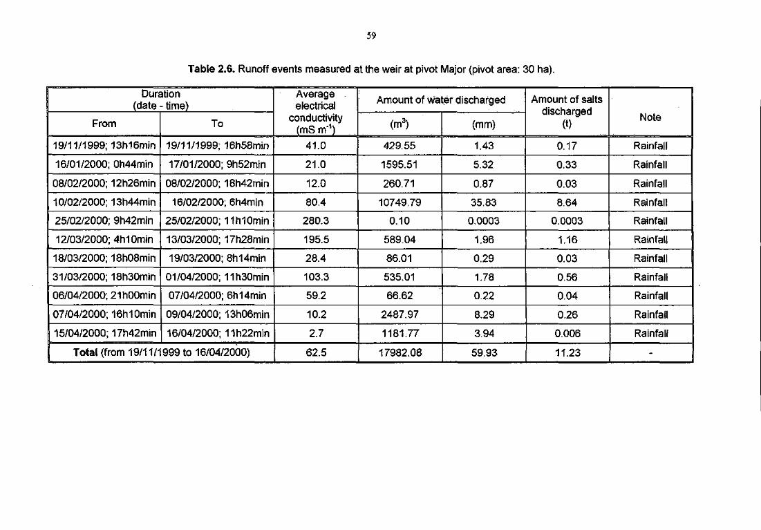
59

Table 2.6. Runoff events measured at the weir at pivot Major (pivot area: 30 ha).

Duration(date - time)

From

19/11/1999; 13h16min

16/01/2000; 0h44min

08/02/2000; 12h26min

10/02/2000; 13h44min

25/02/2000; 9h42min

12/03/2000; 4h10min

18/03/2000; 18hO8min

31/03/2000; 18h30min

06/04/2000; 21 hOOmin

07/04/2000; 16h10min

15/04/2000; 17h42min

To

19/11/1999; 16h58min

17/01/2000; 9h52min

08/02/2000; 18h42min

16/02/2000; 6h4min

25/02/2000; 11h10min

13/03/2000; 17h28min

19/03/2000; 8h14min

01/04/2000; 11h30min

07/04/2000; 6h14min

09/04/2000; 13hO6min

16/04/2000; 11 h22min

Total (from 19/11/1999 to 16/04/2000)

Average -electrical

conductivity(mSnry

41.0

21.0

12.0

80.4

280.3

195.5

28.4

103.3

59.2

10.2

2.7

62.5

Amount of water discharged

(m3)

429.55

1595.51

260.71

10749.79

0.10

589.04

86.01

535.01

66.62

2487.97

1181.77

17982.08

(mm)

1.43

5.32

0.87

35.83

0.0003

1.96

0.29

1.78

0.22

8.29

3.94

59.93

Amount of saltsdischarged

(t)

0.17

0.33

0.03

8.64

0.0003

1.16

0.03

0.56

0.04

0.26

0.006

11.23

Note

Rainfall

Rainfall

Rainfall

Rainfall

Rainfall

Rainfall

Rainfall

Rainfall

Rainfall

Rainfall

Rainfall

-

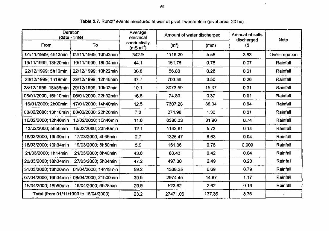
60

Table 2.7. Runoff events measured at weir at pivot Tweefontein (pivot area: 20 ha).

Duration(date - time)

From

01/11/1999; 4h13min

19/11/1999; 13h20min

22/12/1999; 5h10min

23/12/1999; 1h18min

28/12/1999; 18h56min

06/01/2000; 16h10min

16/01/2000; 2h00min

08/02/2000; 13h18min

10/02/2000; 12h46min

13/02/2000; 5h56min

16/03/2000; 19h30min

18/03/2000; 19h34min

21/03/2000; 1h14min

26/03/2000; 18h34min

31/03/2000; 13h20min

07/04/2000; 16h34min

15/04/2000; 18h50min

To

02/11/1999; 10h33min

19/11/1999; 18hO4min

22/12/1999; 10h22min

23/12/1999; 12h46min

29/12/1999; 10h02min

06/01/2000; 22h32min

17/01/2000; 14h40min

08/02/2000; 22h26min

12/02/2000; 10h46min

13/02/2000; 23h40min

17/03/2000; 4h36min

19/03/2000; 5h50min

21/03/2000; 8h40min

27/03/2000; 5h34min

01/04/2000; 14h18min

08/04/2000; 21 hOOmin

16/04/2000; 6h28min

Total (from 01/11/1999 to 16/04/2000)

Averageelectrical

conductivity(mS m'1)

342.9

44.1

30.8

37.7

10.1

16.6

12.5

7.3

11.6

12.1

2.7

5.9

43.8

47.2

59.2

39.6

29.9

23.2

Amount of water discharged

(m3)

1116.20

151.75

56.88

700.36

3073.59

74.80

7607.28

271.98

6380.33

1143.91

1325.47

151.36

83.43

497.30

1338.35

2974.45

523.62

27471.06

(mm)

5.58

0.76

0.28

3.50

15.37

0.37

38.04

1.36

31.90

5.72

6.63

0.76

0.42

2.49

6.69

14.87

2.62

137.36

Amount of saltsdischarged

<t)

3.83

0.07

0.01

0.26

0.31

0.01

0.94

0.01

0.74

0.14

0.04

0.009

0.04

0.23

0.79

1.17

0.16

8.76

Note

Over-irrigation

Rainfall

Rainfall

Rainfall

Rainfall

Rainfall

Rainfall

Rainfall

Rainfall

Rainfall

Rainfall

Rainfall

Rainfall

Rainfall

Rainfall

Rainfall

Rainfall

-

61

2.3.4.3. Groundwater

2.3.4.3.1. Groundwater quality

Piezometer installations are done through the introduction of foreign material into theboreholes. Great care is usually taken to ensure that groundwater is not undulycontaminated during these installations. A certain degree of contamination is, however,unavoidable, since sodium bentonite is one of the prime materials used to hydraulicallyisolate one horizon from another.

After the installation of a bentonite plug, boreholes have to be flushed, usually over a periodof months, to ensure that all free salts from the bentonite are leached.

In the case of the monitoring holes in the irrigation area, periodic flushing was necessary forthree months after piezometer installation. The results from chemical analyses during thisperiod have therefore been ignored, since they do not reflect the true composition of thegroundwater. Even after this period, traces of abnormal sodium levels were still detected inboreholes BH4 and BH7.

The results from the chemical analyses are presented in Appendix J. Figures 2.63 to 2:65summarize some of the relevant information.

Conclusions from this information are:

• Boreholes BH2 and BH8 showed an increase in nitrate concentrations. Nitrate wasthe most mobile constituent available in the irrigation system and was derived fromfertilizer. The mine water did not contain nitrate concentrations at these levels.

• Boreholes BH2, BH3, BH5, BH8 and BH9 showed a general but small increase incalcium, magnesium and sulphate.

• Boreholes BH4, BH6 and BH7 showed no increase in any of its constituents.

• These response patterns are typical of what can be expected in a geologicalenvironment such as the irrigation pivot. Water from the irrigated area will infiltratealong preferred pathways, thus contaminating the aquifer in a patchy manner.

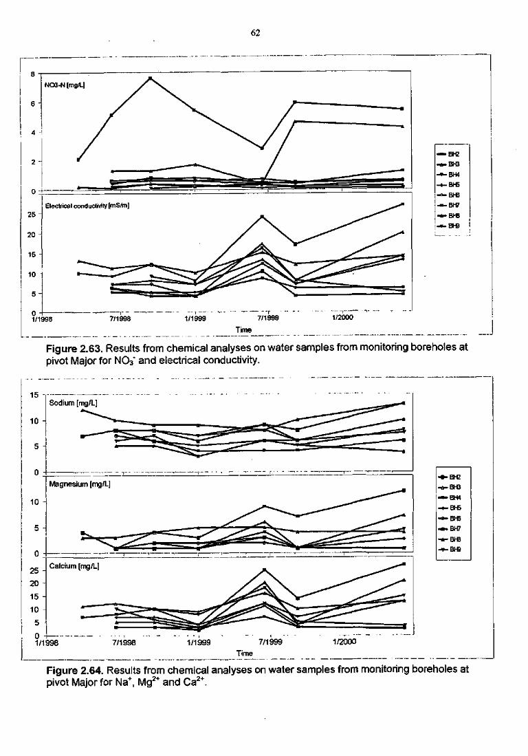
62

-O-BH3

-•-BH4

-t-BI-5

— BH7

-«-BhQ

1/1998 7/1998 1/1999 7/1999 1/2000

Time JFigure 2.63. Results from chemical analyses on water samples from monitoring boreholes atpivot Major for NO3" and electrical conductivity.

7/1998 1/1999 7/1999 1/2000

Time

Figure 2.64. Results from chemical analyses on water samples from monitoring boreholes atpivot Major for Na+, Mg2+ and Ca2+.

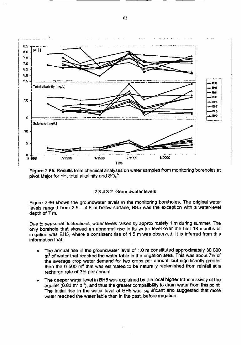
63

8.5

— BH2

-O-BH3

-•-BH4

_j_BH5

— Bl-B

— BH7— BHB-• -BH9

7/1998 1/1999 7/1999 1/2000Time

Figure 2.65. Results from chemical analyses on water samples from monitoring boreholes atpivot Major for pH, total alkalinity and SO4

2".

2.3.4.3.2. Groundwater levels

Figure 2.66 shows the groundwater levels in the monitoring boreholes. The original waterlevels ranged from 2.5 - 4.8 m below surface; BH5 was the exception with a water-leveldepth of 7 m.

Due to seasonal fluctuations, water levels raised by approximately 1 m during summer. Theonly borehole that showed an abnormal rise in its water level over the first 18 months ofirrigation was BH5, where a consistent rise of 1.5 m was observed. It is inferred from thisinformation that:

• The annual rise in the groundwater level of 1.0 m constituted approximately 30 000m3 of water that reached the water table in the irrigation area. This was about 7% ofthe average crop water demand for two crops per annum, but significantly greaterthan the 6 500 m3 that was estimated to be naturally replenished from rainfall at arecharge rate of 3% per annum.

• The deeper water level in BH5 was explained by the local higher transmissivity of theaquifer (0.83 mz d"1), and thus the greater compatibility to drain water from this point.The initial rise in the water level at BH5 was significant and suggested that morewater reached the water table than in the past, before irrigation.

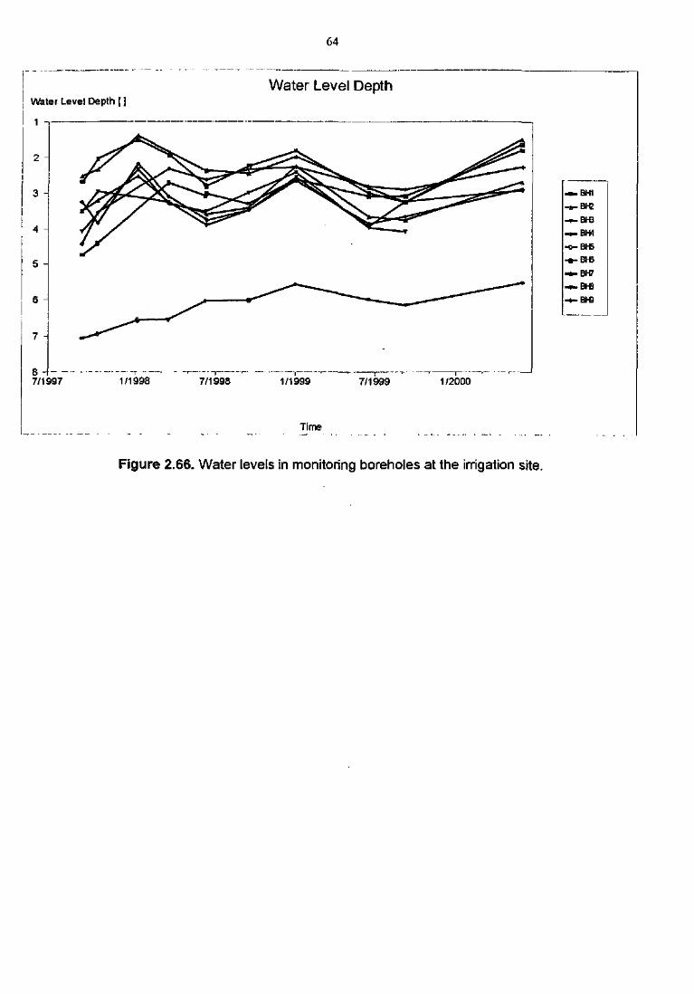
64

Water Level Depth [ ]

1

Water Level Depth

2

3 H

5 -

7 -

8 -f- -7/1997 1 /1998

— BH1

-a-BHE

-*-BH3

-t-B-M

•O-BH5

-«-BH3

-*-BH?

^ " DTD

7/1998 1/1999 7/1999 1/2000

Time

Figure 2.66. Water levels in monitoring boreholes at the irrigation site.

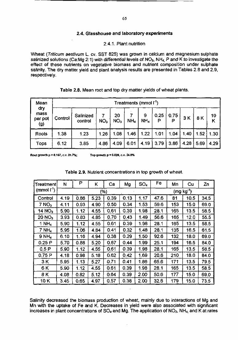
65

2.4. Glasshouse and laboratory experiments

2.4.1. Plant nutrition

Wheat (Triticum aestivum L cv. SST 825) was grown in calcium and magnesium sulphatesalinized solutions (Ca:Mg 2:1) with differential levels of NO3, NH4, P and K to investigate theeffect of these nutrients on vegetative biomass and nutrient composition under sulphatesalinity. The dry matter yield and plant analysis results are presented in Tables 2.8 and 2.9,respectively.

Table 2.8. Mean root and top dry matter yields of wheat plants.

Meandry

massper pot

(g)

Roots

Tops

Treatments (mmol I"1)

Control

1.38

6.12

Salinizedcontrol :

1.23

3.85

7NO3

1.26

4.86

20NO3

1.08

4.09

7NH4

1.46

6.01

9NH4

1.22

4.19

0.25P

1.01

3.79

0.75P

1.04

3.86

3 K

1.40

4.28

8 K

1.52

5.69

10K

1.30

4.29

Root growth p = 0.167, cv. 21.7%; Top growth p = 0.029, cv. 24.8%

Table 2.9. Nutrient concentrations in top growth of wheat.

Treatmenti (mmol r1)

Control7NO3

14NO3

2ONO31 NH4

7NH 4

9NH 4

0.25 P0.5 P

0.75 P3 K6 K8 K10 K

N P K Ca Mg SO4

4.194.115.903.935.905.956.105.705.904.185.955.904.083.45

0.860.93

1.120.83

1.121.061.160.88

1.120.98

1.131.120.820.65

5.234.904.554.854.55

4.844.945.204.555.185.274.555.124.97

0.390.500.610.700.610.410.380.670.610.620.710.61

0.640.57

0.130.340.390.430.390.320.290.440.390.420.410.390.390.38

1.171.531.981.491.981.481.501.991.981.691.861.982.002.00

Fe Mn Cu Zn

(mg kg*1):

47.659.628.156.628.128.192.625.128.120.665.628.1

50.632.6

81153165165165135132194165210

171165177

179

10.515.013.512.013.516.518.016.513.518.013.513.515.015.0

34.569.058.555.558.561.569.084.058.584.079.558.569.073.5

Salinity decreased the biomass production of wheat, mainly due to interactions of Mg andMn with the uptake of Fe and K. Decreases in yield were also associated with significantincreases in plant concentrations of SO4 and Mg. The application of NO3, NH4, and K at rates

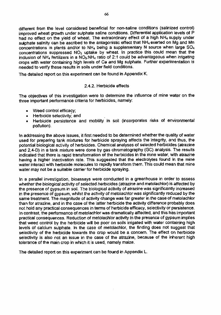
66

different from the level considered beneficial for non-saline conditions (salinized control)improved wheat growth under sulphate saline conditions. Differential application levels of Phad no effect on the yield of wheat. The extraordinary effect of a high NH4 supply undersulphate salinity can be ascribed to the antagonistic effect that NH4 exerted on Mg and Mnconcentrations in plants and/or to NH4 being a supplementary N source when large SO4

concentrations suppressed NO3 uptake by wheat. In practice this could mean that theinclusion of NH4 fertilizers in a NO3:NH4 ratio of 2:1 could be advantageous when irrigatingcrops with water containing high levels of Ca and Mg sulphate. Further experimentation isneeded to verify these results in soils under field conditions.

The detailed report on this experiment can be found in Appendix K.

2.4.2. Herbicide effects

The objectives of this investigation were to determine the influence of mine water on thethree important performance criteria for herbicides, namely:

• Weed control efficacy;• Herbicide selectivity; and• Herbicide persistence and mobility in soil (incorporates risks of environmental

pollution).

In addressing the above issues, it first needed to be determined whether the quality of waterused for preparing tank mixtures for herbicide spraying affects the integrity, and thus, thepotential biological activity of herbicides. Chemical analyses of selected herbicides (atrazineand 2,4-D) in a tank mixture were done by gas chromatography (GC) analysis. The resultsindicated that there is rapid transformation of the herbicides in the mine water, with atrazinehaving a higher inactivation rate. This suggested that the electrolytes found in the minewater interact with herbicide molecules to rapidly transform them. This could mean that minewater may not be a suitable carrier for herbicide spraying.

In a parallel investigation, bioassays were conducted in a greenhouse in order to assesswhether the biological activity of selected herbicides (atrazine and metolachlor) is affected bythe presence of gypsum in soil. The biological activity of atrazine was significantly increasedin the presence of gypsum, whilst the activity of metolachlor was significantly reduced by thesame treatment. The magnitude of activity change was far greater in the case of metolachlorthan for atrazine, and in the case of the latter herbicide the activity difference probably doesnot hold any practical consequences in terms of herbicide efficacy, selectivity or persistence.In contrast, the performance of metolachlor was dramatically affected, and this has importantpractical consequences. Reduction of metolachlor activity in the presence of gypsum impliesthat weed control by the herbicide will be poor on soils irrigated with water containing highlevels of calcium sulphate. In the case of metolachlor, the finding does not suggest thatselectivity of the herbicide towards the crop would be a concern. The effect on herbicideselectivity is also not an issue in the case of the atrazine, because of the inherent hightolerance of the main crop in which it is used, namely maize.

The detailed report on this experiment can be found in Appendix L.

67

CHAPTER 3

3. SOIL WATER BALANCE MODEL

3.1. Model description

Soil Water Balance (SWB) is a mechanistic, multi-layer, daily time step, soil water-salt balance-generic crop growth model, developed from NEWSWB, a modified version of the modelpublished by Campbell and Diaz (1988).

The first components of the soil water balance, which are calculated on a daily time step, arecanopy interception of water and surface runoff. Water infiltration and redistribution can then becalculated using either a cascading soil water balance or a finite-difference water movementmodule based on Richards' equation. In the case of the cascading water balance, saltredistribution is determined assuming complete mixing of irrigation and rainfall with the soilsolution of the topsoil layer, and similarly for the solution percolating to the next lower soil layerand so on. In the case of the finite-difference model, salt redistribution is solved using aconvection/dispersion equation. The salt redistribution subroutine of the finite-difference modelis, however, currently being debugged, and was not therefore used in this report. Any water thatpasses beyond the bottom layer is assumed lost to deep percolation. The amount of saltleached is calculated from the amount and quality of the drained water.

Chemical equilibrium is calculated on a daily time step per soil layer, using the model publishedby Robbins (1991). Critical assumptions of the chemical equilibrium model and the validationwith lysimeter data are discussed in the same study. The model of Robbins (1991) solveschemical equilibrium by iteration. Within each iteration, activity coefficients and ion activities arecalculated for Ca2+, Mg2+, Na+, H+, SO4

2', HCO3" and CO32', and the solution phase is

equilibrated with solid phase lime and gypsum, if present. EC is calculated from individual ionconcentrations (McNeal et al., 1970) for each soil layer. The SWB model ends the iterationprocedure when the change in EC between the previous and the following loop is < 0.01 mSm'1.

Potential evapotranspiration (PET) is calculated as a function of daily average air temperature,vapour pressure deficit, radiation and wind speed, adopting the internationally standardizedFAO Penman-Monteith methodology (Allen et al., 1998). The two components of PET (potentialevaporation and potential transpiration) are estimated from canopy cover. Actual transpiration isdetermined on a daily basis as the lesser of root water uptake or maximum loss rate. Total soilwater potential is used to determine the amount of water available for crop transpiration in eachsoil layer. The osmotic effect on crop growth is simulated by adding osmotic potential to thematric and gravitational soil water potentials. Osmotic potential is calculated as a function ofionic concentration (Campbell, 1985). The daily dry matter increment (DM,) is taken as theminimum of the water supply limited (Tanner and Sinclair, 1983) and radiation limited DMj(Monteith, 1977). A stress index, the ratio between actual and potential transpiration, is used asa limiting factor for canopy growth.

Required weather and management input data are planting date, latitude, altitude, rainfall andirrigation water amounts and quality, as well as maximum and minimum daily temperature. Inthe absence of measured data, SWB estimates solar radiation, vapour pressure and wind speedaccording to the FAO recommendations (Allen et al., 1998). Required soil input data are

68

volumetric field capacity, permanent wilting point and a runoff curve number to calculate runoffbased on the SCS method (Stewart et al., 1976). In addition, initial volumetric soil water content,the content of soluble and exchangeable ionic species, as well as initial gypsum and lime arerequired for each soil layer.

If the cascading water redistribution is used, a drainage factor (fraction of water above fieldcapacity that cascades daily to the next layer) and a drainage rate upper limit (maximumamount of water that percolates from the bottom layer in one day) need to be entered. Thefinite-difference model does not need inputs like drainage factor and maximum drainage rate,which are very difficult to estimate in particular for poorly drained soils, but a realisticassumption of the bottom boundary condition is required. If available, measured saturatedhydraulic conductivity can be entered as input for each soil layer when the finite-difference waterbalance is run. Alternatively, the model estimates saturated hydraulic conductivity from fieldcapacity and permanent wilting point using the function of Campbell (1985). Theconvection/dispersion equation also requires dispersivity factors for each ionic species.

The SWB model is written in Delphi v. 5.0 (Inprise Corp.) and runs in a user-friendly Windows95 environment. A full description of the model before the improvements made during thecourse of this project, can be found in Annandale et al. (1999b). The SWB model includesspecific crop growth parameters for a wide range of species (Annandale et al., 1999b).

Weather data are generated using CLIMGEN, a two-component weather generator developedby GS Campbell (Washington State University) and based on the work of Richardson andWright (1984). The first component (CLIMPAR) determines statistical parameters required forlong-term daily weather data generation, while the second component (CLIMGEN) generatesweather data. CLIMGEN generates daily maximum and minimum air temperature, as well asprecipitation from either historic daily weather data, if available, or from monthly averages. Atleast 20 years of rainfall and 10 years of historic temperature data are required in order to get areliable simulation. The CLIMGEN weather data generator was assessed at South African sitesby Clemence (1997), who showed the estimations to be quite satisfactory.

CLIMGEN is also written in Delphi v. 5.0 and runs in a user-friendly Windows 95 format. Thedatabase of CLIMGEN can be used as the weather database of SWB.

Improvements to the SWB model

The following improvements have been made to the SWB model during the course of thisproject:

i) The finite-difference water balance subroutine based on Richards' equation wasincluded in the SWB model. This was done during the study leave of the projectleader at CSiRO (Townsville, Australia). The finite-difference water redistributionimproves the simulations as water moves both upwards and downwards drivenby soil matric potential gradients. The theory of the finite-difference waterredistribution model is reported in Appendix M.

ii) The salt redistribution in the finite-difference water balance model can besimulated using the convection/dispersion equation. The code was also writtenduring the study leave of the project leader at CSIRO. The convection/dispersionequation is expected to improve the simulation of salt redistribution as salts aremoved by mass flow or convection, as well as by diffusion in response to

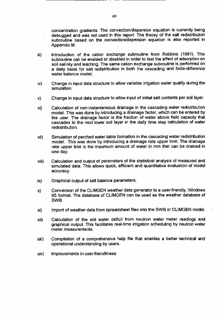
69

concentration gradients. The convection/dispersion equation is currently beingdebugged and was not used in this report. The theory of the salt redistributionsubroutine based on the convection/dispersion equation is also reported inAppendix M.

iii) Introduction of the cation exchange subroutine from Robbins (1991). Thissubroutine can be enabled or disabled in order to test the effect of adsorption onsoil salinity and leaching. The same cation exchange subroutine is performed ona daily basis for salt redistribution in both the cascading and finite-differencewater balance model.

iv) Change in input data structure to allow variable irrigation water quality during thesimulation.

v) Change in input data structure to allow input of initial salt contents per soil layer.

vi) Calculation of non-instantaneous drainage in the cascading water redistributionmodel. This was done by introducing a drainage factor, which can be entered bythe user. The drainage factor is the fraction of water above field capacity thatcascades to the next lower soil layer in the daily time step calculation of waterredistribution.

vii) Simulation of perched water table formation in the cascading water redistributionmodel. This was done by introducing a drainage rate upper limit. The drainagerate upper limit is the maximum amount of water in mm that can be drained inone day.

viii) Calculation and output of parameters of the statistical analysis of measured andsimulated data. This allows quick, efficient and quantitative evaluation of modelaccuracy.

ix) Graphical output of salt balance parameters.

x) Conversion of the CLIMGEN weather data generator to a user-friendly, Windows95 format. The database of CLIMGEN can be used as the weather database ofSWB.

xi) Import of weather data from spreadsheet files into the SWB or CLIMGEN model.

xii) Calculation of the soil water deficit from neutron water meter readings andgraphical output. This facilitates real-time irrigation scheduling by neutron watermeter measurements.

xiii) Compilation of a comprehensive help file that enables a better technical andoperational understanding by users.

xiv) Improvements in user-friendliness.

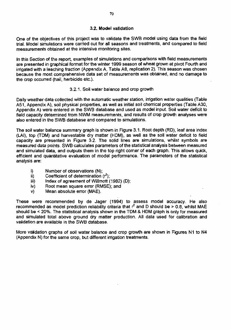
70

3.2. Model validation

One of the objectives of this project was to validate the SWB model using data from the fieldtrial. Model simulations were carried out for all seasons and treatments, and compared to fieldmeasurements obtained at the intensive monitoring sites.

In this Section of the report, examples of simulations and comparisons with field measurementsare presented in graphical format for the winter 1999 season of wheat grown at pivot Fourth andirrigated with a leaching fraction (Appendix A, Table A8, replication 2). This season was chosenbecause the most comprehensive data set of measurements was obtained, and no damage tothe crop occurred (hail, herbicide etc.).

3.2.1. Soil water balance and crop growth

Daily weather data collected with the automatic weather station, irrigation water qualities (TableA51, Appendix A), soil physical properties, as well as initial soil chemical properties (Table A30,Appendix A) were entered in the SWB database and used as model input. Soil water deficit tofield capacity determined from NWM measurements, and results of crop growth analyses werealso entered in the SWB database and compared to simulations.

The soil water balance summary graph is shown in Figure 3.1. Root depth (RD), leaf area index(LAI), top (TDM) and harvestable dry matter (HDM), as well as the soil water deficit to fieldcapacity are presented in Figure 3.2. The solid lines are simulations, whilst symbols aremeasured data points. SWB calculates parameters of the statistical analysis between measuredand simulated data, and outputs them in the top right corner of each graph. This allows quick,efficient and quantitative evaluation of model performance. The parameters of the statisticalanalysis are:

i) Number of observations (N);ii) Coefficient of determination (r2);iii) Index of agreement of Willmott (1982) (D);iv) Root mean square error (RMSE); andv) Mean absolute error (MAE).

These were recommended by de Jager (1994) to assess model accuracy. He alsorecommended as model prediction reliability criteria that r2 and D should be > 0.8, whilst MAEshould be < 20%. The statistical analysis shown in the TDM & HDM graph is only for measuredand simulated total above ground dry matter production. All data used for calibration andvalidation are available in the SWB database.

More validation graphs of soil water balance and crop growth are shown in Figures N1 to N4(Appendix N) for the same crop, but different irrigation treatments.

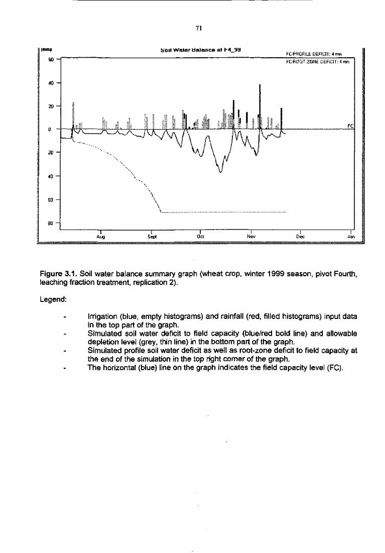
71

Qc; Nov Dee •Jan

Figure 3.1. Soil water balance summary graph (wheat crop, winter 1999 season, pivot Fourth,leaching fraction treatment, replication 2).

Legend:

Irrigation (blue, empty histograms) and rainfall (red, filled histograms) input datain the top part of the graph.Simulated soil water deficit to field capacity (blue/red bold line) and allowabledepletion level (grey, thin line) in the bottom part of the graph.Simulated profile soil water deficit as well as root-zone deficit to field capacity atthe end of the simulation in the top right corner of the graph.The horizontal (blue) line on the graph indicates the field capacity level (FC).

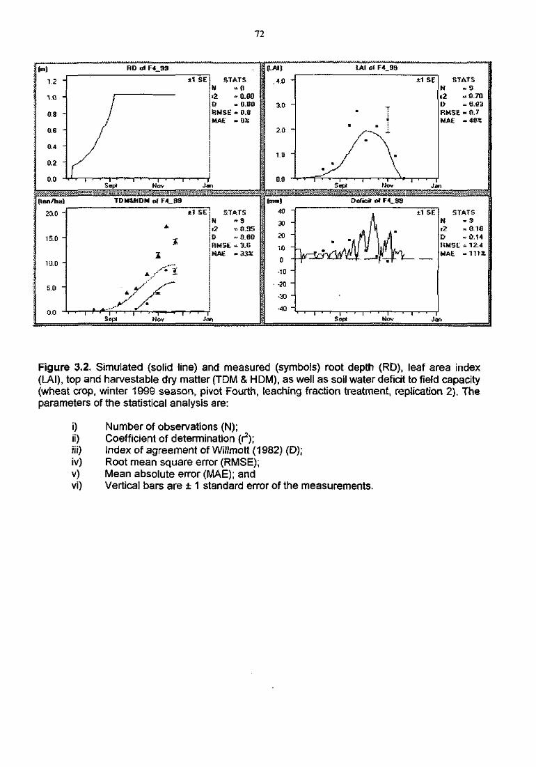
72

Hm)

i 1.2 "

i 1.0 -

\ 0.8 "

;! 0.6 -

i 0.4 "

i 0.2 "

J 0.0

i (inn/ha)

- 2ao -

1 15.0 "

'•• ia D •

\ 5.0 -

\ o.o -

RD of F4_33

//

/

jJ

f• • \ ' ' ! ' ' i ' • i •

Sept NovW w S ' i v - ' S •'.•?£• io'^'o1-"- ••••• •*• "Wvv i*+": "̂ ;"'-w:"' •S^::-;; :¥; •£• I '^ ' fe

TDMtHDM of F-1_.SJ

*

2

Sept Nov

±1 SEU

(2B

STATS

^ U.00ise - o.c

Jan

I

±1 SE!

r2

»».

Jon

STATS- S.. 0.35--• B.88

iSEJ i ' j i !tt »3SS

• (LAI)

3 4.0

^ 3.0

j 20

1.0

5 0.0

: 40

30

20

) o-10

• -20

-30

•40

LAI of F4_33

-

-

-

±1 SE

• ;

a

/ ' ^

_>>/ \

STATSH -5t2 " 0.70D - 0.83KMSt - 0.7MAE - 4BX

• • , • . | • . J • , . r- j , [

Sept Ho* Jon

Deficit of F4_3S

-

_

-

-

-

-

-

, ±1 SE

\\ y iijv

I I 1 • I . . . . . . 1 . , . . ,

STATS

r2 - 0.18D nr 0.14KMSt - 12.4MAE -111X

Sept Nov Jari

Figure 3.2. Simulated (solid line) and measured (symbols) root depth (RD), leaf area index(LAI), top and harvestable dry matter (TDM & HDM), as well as soil water deficit to field capacity(wheat crop, winter 1999 season, pivot Fourth, leaching fraction treatment, replication 2). Theparameters of the statistical analysis are:

i) Number of observations (N);ii) Coefficient of determination (r2);iii) Index of agreement of Willmott (1982) (D);iv) Root mean square error (RMSE);v) Mean absolute error (MAE); andvi) Vertical bars are ± 1 standard error of the measurements.

73

The growth parameters for wheat used in these simulations were obtained from the database ofSWB (Annandale et al., 1999b). A slight modification was introduced to correct the thermal timerequirements for crop developmental stages, and dry matter partitioning in order to simulatemore accurately the development and growth of the particular cultivar.

The statistical analysis indicated that the simulated and measured data were generally inside ormarginally outside the established criteria. Discrepancies were mainly due to spatial variabilityfor crop growth parameters (LAI, TDM and HDM). Large MAE was observed for soil water deficitto field capacity for the leaching fraction treatment (Figure 3.2), as the values were generallyclose to 0.

3.2.2. Soil water redistribution

A detailed validation of water redistribution was carried out by comparing simulated values ofsoil matric potential to those obtained with the heat dissipation sensors. The heat dissipationsensors were individually calibrated and their readings normalized for soil temperature at 20 °Cusing the procedure described by Campbell et al. (2001).

The CS-615 soii reflectometers, which were installed in the field in the first three seasons of thetrial, proved to be unsuitable for this type of experiment, as it was impossible to separate out theeffects of volumetric soil water content and soil salinity on their readings. The reflectometerswere therefore replaced by the TDR system, which should provide measurement of volumetricsoil water content and electrical conductivity of the soil solution separately. However, the TDRtechnique was still under development at the time of compilation of this report.

Figure 3.3 presents the comparison between simulated and measured soil matric potentials,where simulated values were obtained using both the cascading and the finite-difference model.The comparison was done for 16 cm soil depth, where soil water redistribution is more dynamiccompared to deeper soil layers due to infiltration and evaporation fluxes. Simulated data of soilmatric potential generally compared very well to field measurements. It is interesting to note thesensitivity of the sensors and the model response to irrigation and rainfall events. The finite-difference model proved to be more dynamic than the cascading model, as can be seen fromthe trend of the simulation line. The finite-difference model moves water both downwards andupwards according to matric potential gradients. The simulation with the finite-difference model,however, was carried out without any effect of salts, as the convection/dispersion saltredistribution subroutine is currently being debugged. The finite-difference model has potentialto predict the soil and salt water baJance more accurately than the cascading model, once thesalt redistribution subroutine is included in SWB.

More validation data of soil water redistribution are shown in Appendix N (Figures N5 to N10) forthe same crop, but different irrigation treatments and soil depths.

A summary of the seasonal soil water balances predicted with the cascading model for all pivotsand treatments is included in Tables 3.1 to 3.4. Rainfall and irrigation were measured withtipping bucket rain gauges at all intensive monitoring stations. Less irrigation was generallyapplied during the rainy summer seasons. In particular, very little irrigation was applied duringthe 1999/00 season, which was extremely wet. The SWB model was used to split the waterbalance losses between soil evaporation, crop transpiration, drainage, canopy interception aswell as surface and subsurface runoff. Soil evaporation and crop transpiration depended onplant species and canopy cover. Drainage varied at pivots Major and Fourth (Tables 3.1 and3.4) depending on rainfall. In particular, considerable amounts of water were predicted to have

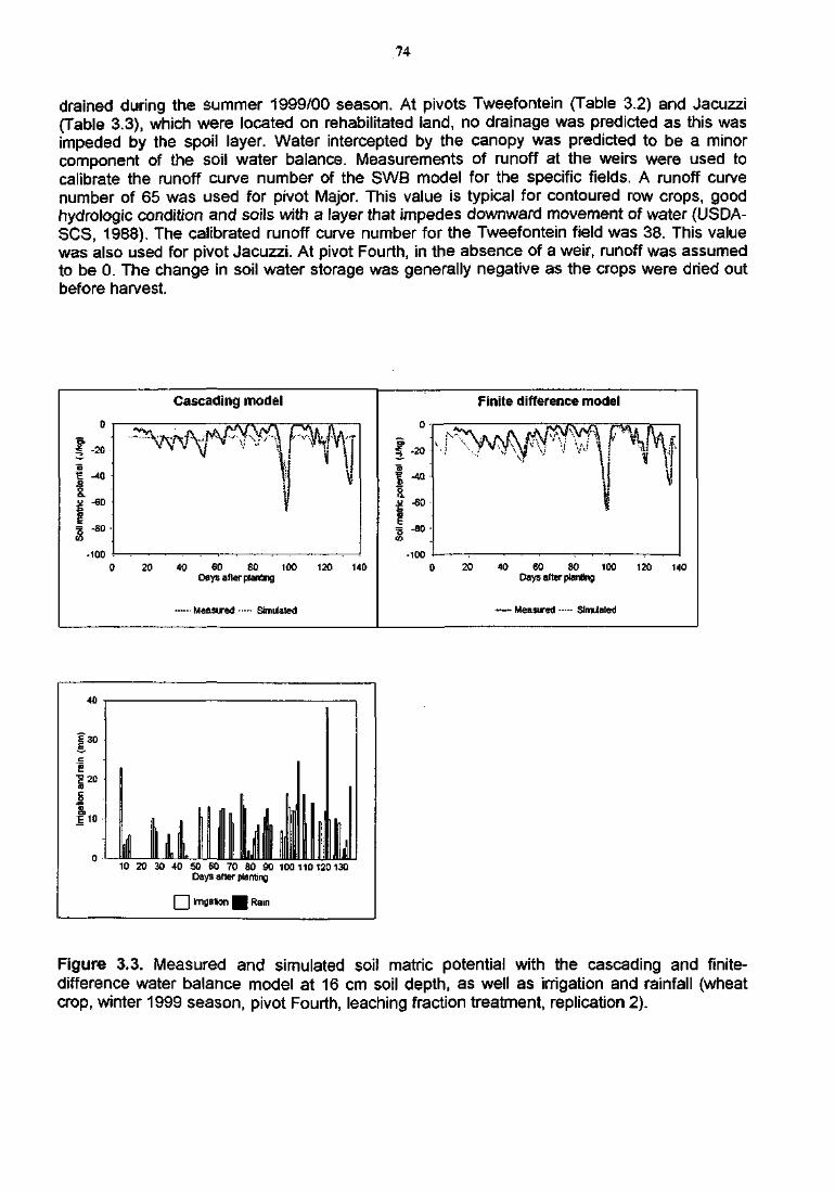
74

drained during the summer 1999/00 season. At pivots Tweefontein (Table 3.2) and Jacuzzi(Table 3.3), which were located on rehabilitated land, no drainage was predicted as this wasimpeded by the spoil layer. Water intercepted by the canopy was predicted to be a minorcomponent of the soil water balance. Measurements of runoff at the weirs were used tocalibrate the runoff curve number of the SWB model for the specific fields. A runoff curvenumber of 65 was used for pivot Major. This value is typical for contoured row crops, goodhydrologic condition and soils with a layer that impedes downward movement of water (USDA-SCS, 1988). The calibrated runoff curve number for the Tweefontein field was 38. This valuewas also used for pivot Jacuzzi. At pivot Fourth, in the absence of a weir, runoff was assumedto be 0. The change in soil water storage was generally negative as the crops were dried outbefore harvest.

0

1 - 2 0

? -40

I

S -80

• 100 L

0

Cascading model

20 40 60 SO 100 120 140Days after planing

Measured Simulated

Finite difference modet

-10020 40 60 80 100 120 140

Days after platting

• Measured Simulated

40

10 20 30 40 50 60 70 80 90 100 110 120130Days after planting

I I Imgation • Rain

Figure 3.3. Measured and simulated soil matric potential with the cascading and finite-difference water balance model at 16 cm soil depth, as well as irrigation and rainfall (wheatcrop, winter 1999 season, pivot Fourth, leaching fraction treatment, replication 2).

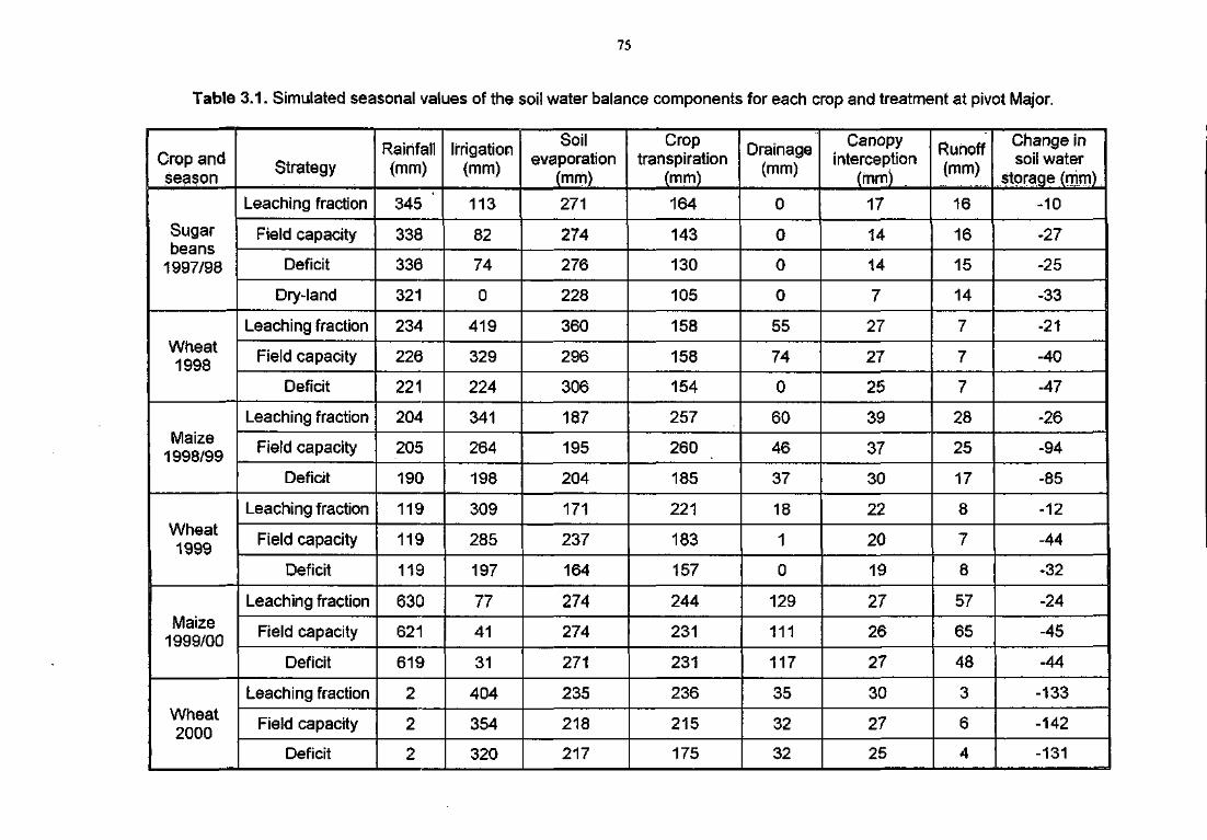
75

Table 3.1. Simulated seasonal values of the soil water balance components for each crop and treatment at pivot Major.

Crop andseason

Sugarbeans

1997/98

Wheat1998

Maize1998/99

Wheat1999

Maize1999/00

Wheat2000

Strategy

Leaching fraction

Field capacity

Deficit

Dry-land

Leaching fraction

Field capacity

Deficit

Leaching fraction

Field capacity

Deficit

Leaching fraction

Field capacity

Deficit

Leaching fraction

Field capacity

Deficit

Leaching fraction

Field capacity

Deficit

Rainfall(mm)

345 '

338

336

321

234

226

221

204

205

190

119

119

119

630

621

619

2

2

2

Irrigation(mm)

113

82

74

0

419

329

224

341

264

198

309

285

197

77

41

31

404

354

320

Soilevaporation

(mm)

271

274

276

228

360

296

306

187

195

204

171

237

164

274

274

271

235

218

217

Croptranspiration

(mm)

164

143

130

105

158

158

154

257

260

185

221

183

157

244

231

231

236

215

175

Drainage(mm)

0

0

0

0

55

74

0

60

46

37

18

1

0

129

111

117

35

32

32

Canopyinterception

(mm)

17

14

14

7

27

27

25

39

37

30

22

20

19

27

26

27

30

27

25

Runoff(mm)

16

16

15

14

7

7

7

28

25

17

8

7

8

57

65

48

3

6

4

Change insoil water

storage (mm)

-10

-27

-25

-33

-21

-40

-47

-26

-94

-85

-12

-44

-32

-24

-45

-44

-133

-142

-131

76

Table 3.2. Simulated seasonal values of the soil water balance components for each crop and treatment at pivot Tweefontein.

Crop andseason

Sugarbeans1997/98

Wheat1998

Sugarbeans1998/99

Wheat1999Maize

1999/00Wheat2000

Strategy

Leaching fraction

Field capacity

Deficit

Leaching fraction

Fieid capacity

Deficit

Leaching fraction

Field capacity

Deficit

Field capacity

Field capacity

Field capacity

Rainfall(mm)

192

191

194

184

222

201

161

154

156

132

668

2

Irrigation(mm)

82

70

59

444

339

208

278

237

199

458

13

615

Soilevaporation

(mm)

188

189

188

386

367

309

288

287

277

314

264

260

Croptranspiration

(mm)

70

70

70

153

153

150

134

106

87

222

225

236

Drainage(mm)

0

0

0

0

0 .

0

0

0

0

0

0

0

Canopyinterception

(mm)

9

9

9

26

27

25

19

16

16

22

26

29

Runoff(mm)

22

20

20

25

19

22

39

34

33

47

130

63

Change insoil waterstorage

(mm)

-15

-27

-34

38

-5

-97

-41

-52

-58

-15

36

29

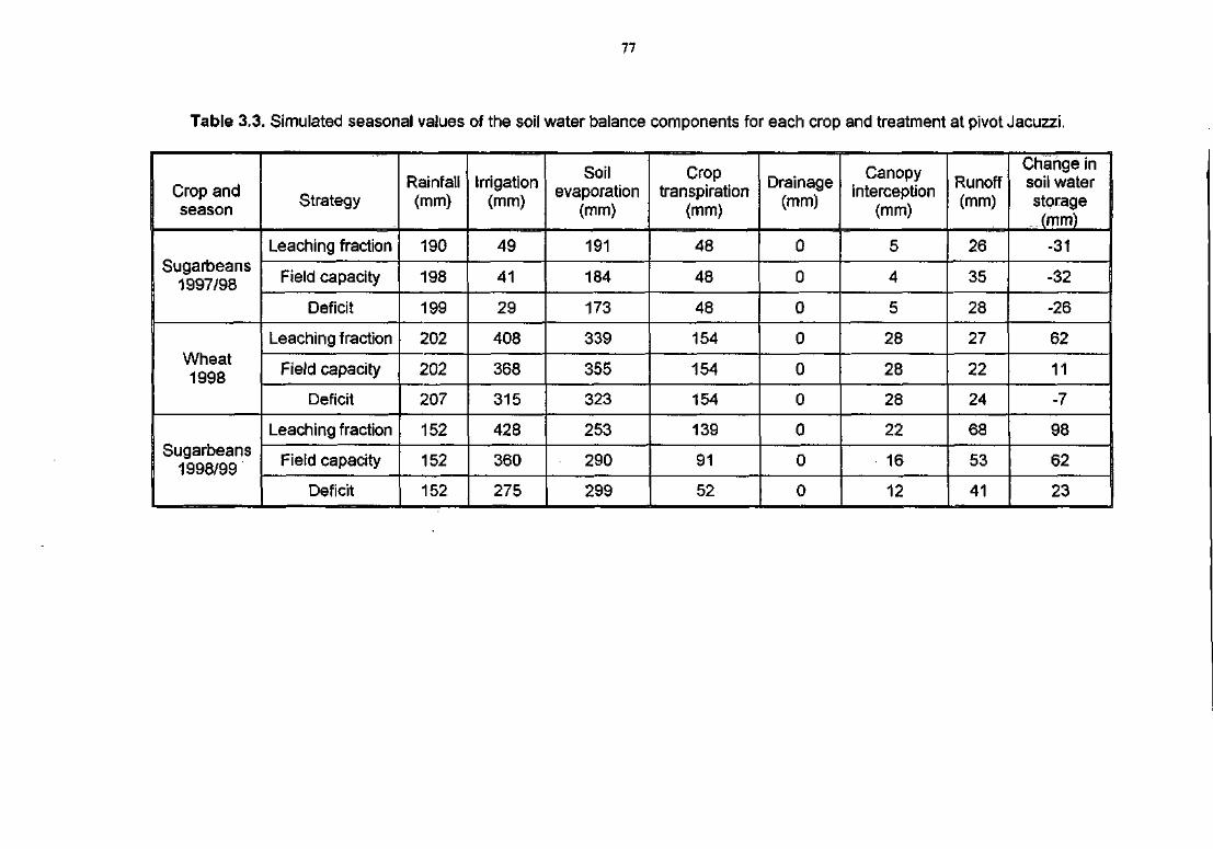
77

Table 3.3. Simulated seasonal values of the soil water balance components for each crop and treatment at pivot Jacuzzi.

Crop andseason

Sugarbeans1997/98

Wheat1998

Sugarbeans1998/99

Strategy

Leaching fraction

Field capacity

Deficit

Leaching fraction

Field capacity

Deficit

Leaching fraction

Field capacity

Deficit

Rainfall(mm)

190

198

199

202

202

207

152

152

152

Irrigation(mm)

49

41

29

408

368

315

428

360

275

Soilevaporation

(mm)

191

184

173

339

355

323

253

290

299

Croptranspiration

(mm)

48

48

48

154

154

154

139

91

52

Drainage(mm)

0

0

0

0

0

0

0

0

0

Canopyinterception

(mm)

5

4

5

28

28

28

22

16

12

Runoff(mm)

26

35

28

27

22

24

68

53

41

Change insoil waterstorage(mm)-31

-32

-26

62

11

-7

98

62

23

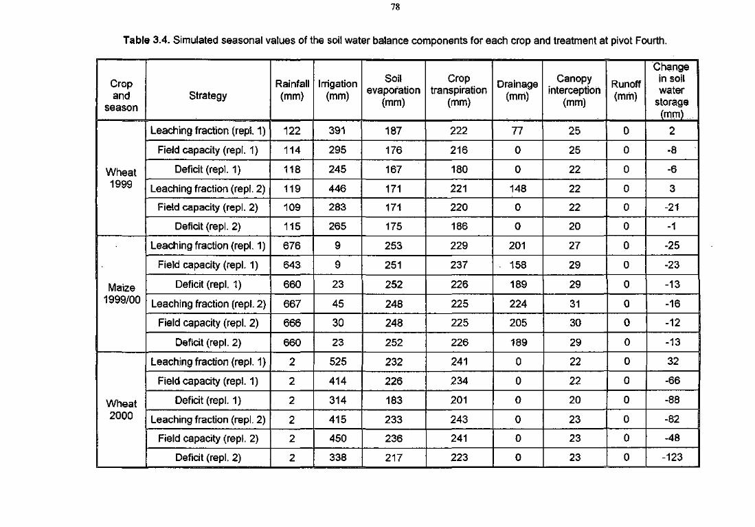
78

Table 3.4. Simulated seasonal values of the soil water balance components for each crop and treatment at pivot Fourth.

Cropand

season

Wheat1999

Maize1999/00

Wheat2000

Strategy

Leaching fraction (repl. 1)

Field capacity (repl. 1)

Deficit (repl. 1)

Leaching fraction (repl. 2)

Field capacity (repl. 2)

Deficit (repl. 2)

Leaching fraction (repl. 1)

Field capacity (repl. 1)

Deficit (repl. 1)

Leaching fraction (repl. 2)

Field capacity (repl. 2)

Deficit (repl. 2)

Leaching fraction (repl. 1)

Field capacity (repl. 1)

Deficit (repl. 1)

Leaching fraction (repl. 2)

Field capacity (repl. 2)

Deficit (repl. 2)

Rainfall(mm)

122

114

118

119

109

115

676

643

660

667

666

660

2

2

2

2

2

2

Irrigation(mm)

391

295

245

446

283

265

9

9

23

45

30

23

525

414

314

415

450

338

Soilevaporation

(mm)

187

176

167

171

171

175

253

251

252

248

248

252

232

226

183

233

236

217

Croptranspiration

(mm)

222

216

180

221

220

186

229

237

226

225

225

226

241

234

201

243

241

223

Drainage(mm)

77

0

0

148

0

0

201

. 158

189

224

205

189

0

0

0

0

0

0

Canopyinterception

(mm)

25

25

22

22

22

20

27

29

29

31

30

29

22

22

20

23

23

23

Runoff(mm)

0

0

0

0

0

0

0

0

0

0

0

0

0

0

0

0

0

0

Changein soilwater

storage(mm)

2

-8

-6

3

-21

-1

-25

-23

-13

-16

-12

-13

32

-66

-88

-82

-48

-123

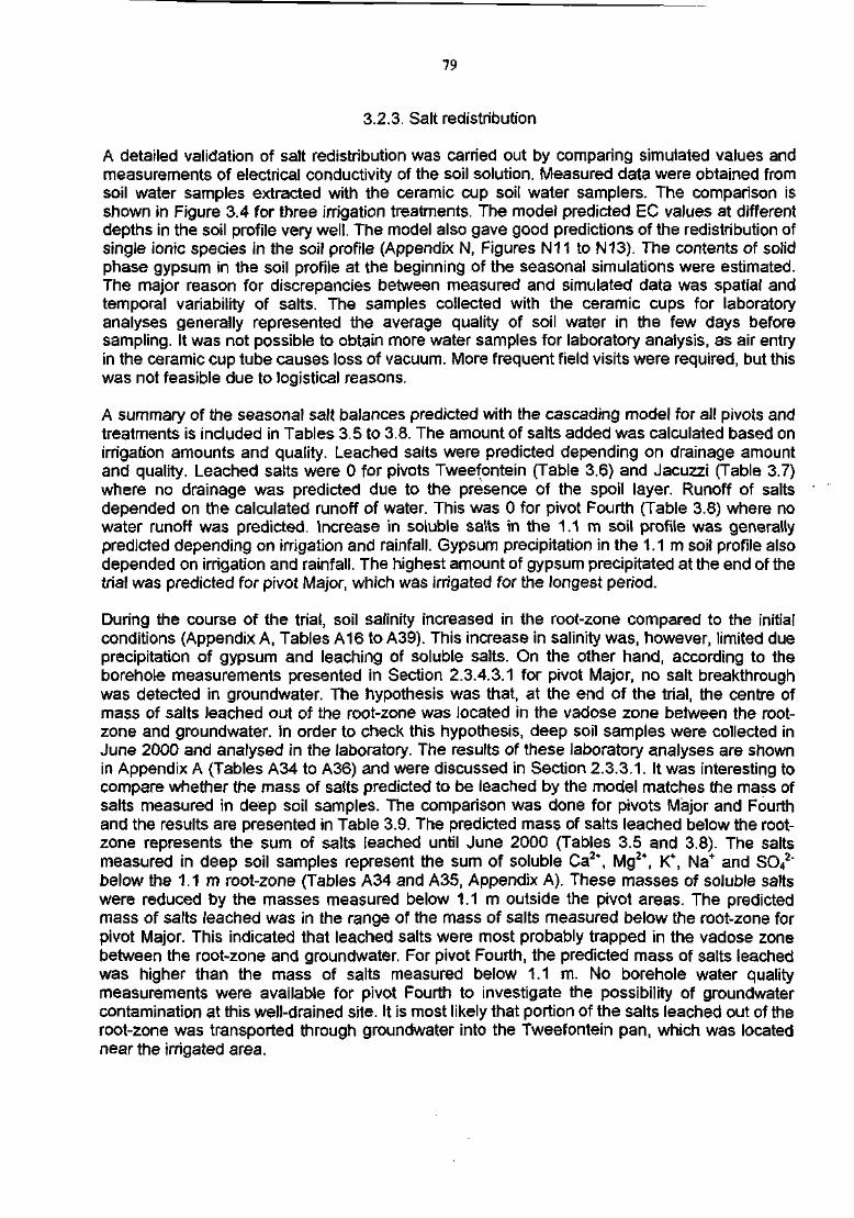
79

3.2.3. Salt redistribution

A detailed validation of salt redistribution was carried out by comparing simulated values andmeasurements of electrical conductivity of the soil solution. Measured data were obtained fromsoil water samples extracted with the ceramic cup soil water samplers. The comparison isshown in Figure 3.4 for three irrigation treatments. The model predicted EC values at differentdepths in the soil profile very well. The model also gave good predictions of the redistribution ofsingle ionic species in the soil profile (Appendix N, Figures N11 to N13). The contents of solidphase gypsum in the soil profile at the beginning of the seasonal simulations were estimated.The major reason for discrepancies between measured and simulated data was spatial andtemporal variability of salts. The samples collected with the ceramic cups for laboratoryanalyses generally represented the average quality of soil water in the few days beforesampling. It was not possible to obtain more water samples for laboratory analysis, as air entryin the ceramic cup tube causes loss of vacuum. More frequent field visits were required, but thiswas not feasible due to logistical reasons.

A summary of the seasonal salt balances predicted with the cascading model for all pivots andtreatments is included in Tables 3.5 to 3.8. The amount of salts added was calculated based onirrigation amounts and quality. Leached salts were predicted depending on drainage amountand quality. Leached salts were 0 for pivots Tweefontein (Table 3.6) and Jacuzzi (Table 3.7)where no drainage was predicted due to the presence of the spoil layer. Runoff of saltsdepended on the calculated runoff of water. This was 0 for pivot Fourth (Table 3.8) where nowater runoff was predicted. Increase in soluble salts in the 1.1 m soil profile was generallypredicted depending on irrigation and rainfall. Gypsum precipitation in the 1.1 m soil profile alsodepended on irrigation and rainfall. The highest amount of gypsum precipitated at the end of thetrial was predicted for pivot Major, which was irrigated for the longest period.

During the course of the trial, soil salinity increased in the root-zone compared to the initialconditions (Appendix A, Tables A16 to A39). This increase in salinity was, however, limited dueprecipitation of gypsum and leaching of soluble salts. On the other hand, according to theborehole measurements presented in Section 2.3.4.3.1 for pivot Major, no salt breakthroughwas detected in groundwater. The hypothesis was that, at the end of the trial, the centre ofmass of salts leached out of the root-zone was located in the vadose zone between the root-zone and groundwater. In order to check this hypothesis, deep soil samples were collected inJune 2000 and analysed in the laboratory. The results of these laboratory analyses are shownin Appendix A (Tables A34 to A36) and were discussed in Section 2.3.3.1. It was interesting tocompare whether the mass of saits predicted to be leached by the model matches the mass ofsalts measured in deep soil samples. The comparison was done for pivots Major and Fourthand the results are presented in Table 3.9. The predicted mass of salts leached below the root-zone represents the sum of salts leached until June 2000 (Tables 3.5 and 3.8). The saltsmeasured in deep soil samples represent the sum of soluble Ca2*, Mg2+, K+, Na+ and SO4

2'below the 1.1 m root-zone (Tables A34 and A35, Appendix A). These masses of soluble saltswere reduced by the masses measured below 1.1 m outside the pivot areas. The predictedmass of salts leached was in the range of the mass of salts measured below the root-zone forpivot Major. This indicated that leached salts were most probably trapped in the vadose zonebetween the root-zone and groundwater. For pivot Fourth, the predicted mass of salts leachedwas higher than the mass of salts measured below 1.1 m. No borehole water qualitymeasurements were available for pivot Fourth to investigate the possibility of groundwatercontamination at this well-drained site. It is most likely that portion of the salts leached out of theroot-zone was transported through groundwater into the Tweefontein pan, which was locatednear the irrigated area.

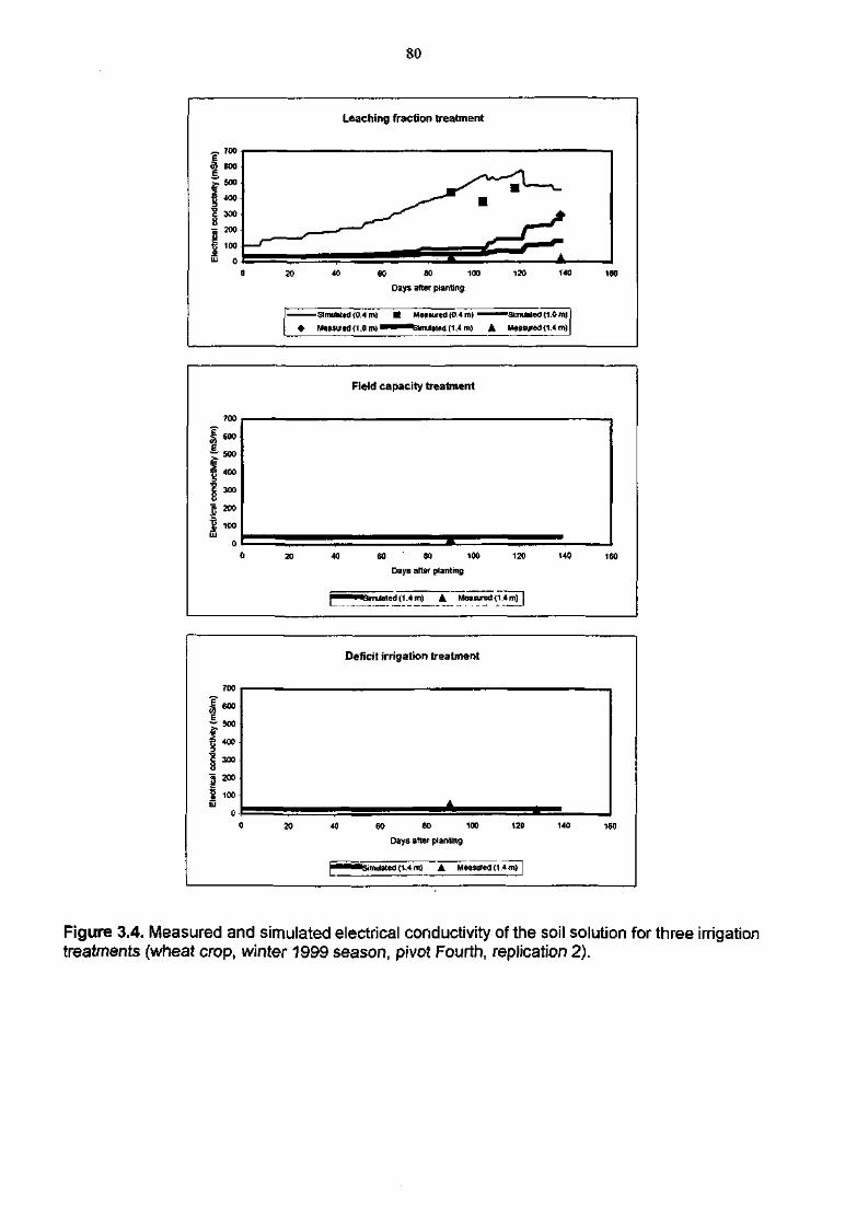
80

Leaching fraction treatment

60 80 100

Days after planting

120 140

Simulated (0.4 m)• Measured n.Om)

•S-rnulato) 11.0 m!led (1.1m) A

II 5 0 0

200

100

Field capacity treatment

80 ' 80 100

Days after plantmg

120 140

A Measued<1.4m) j

160

I 5 0 0400

300

20

Deficit irrigation treatment

M""B*Simuisted (1.4 m) A Measured (i!?n^]

60 80 100 120 140

Days after planting

Figure 3.4. Measured and simulated electrical conductivity of the soil solution for three irrigationtreatments (wheat crop, winter 1999 season, pivot Fourth, replication 2).

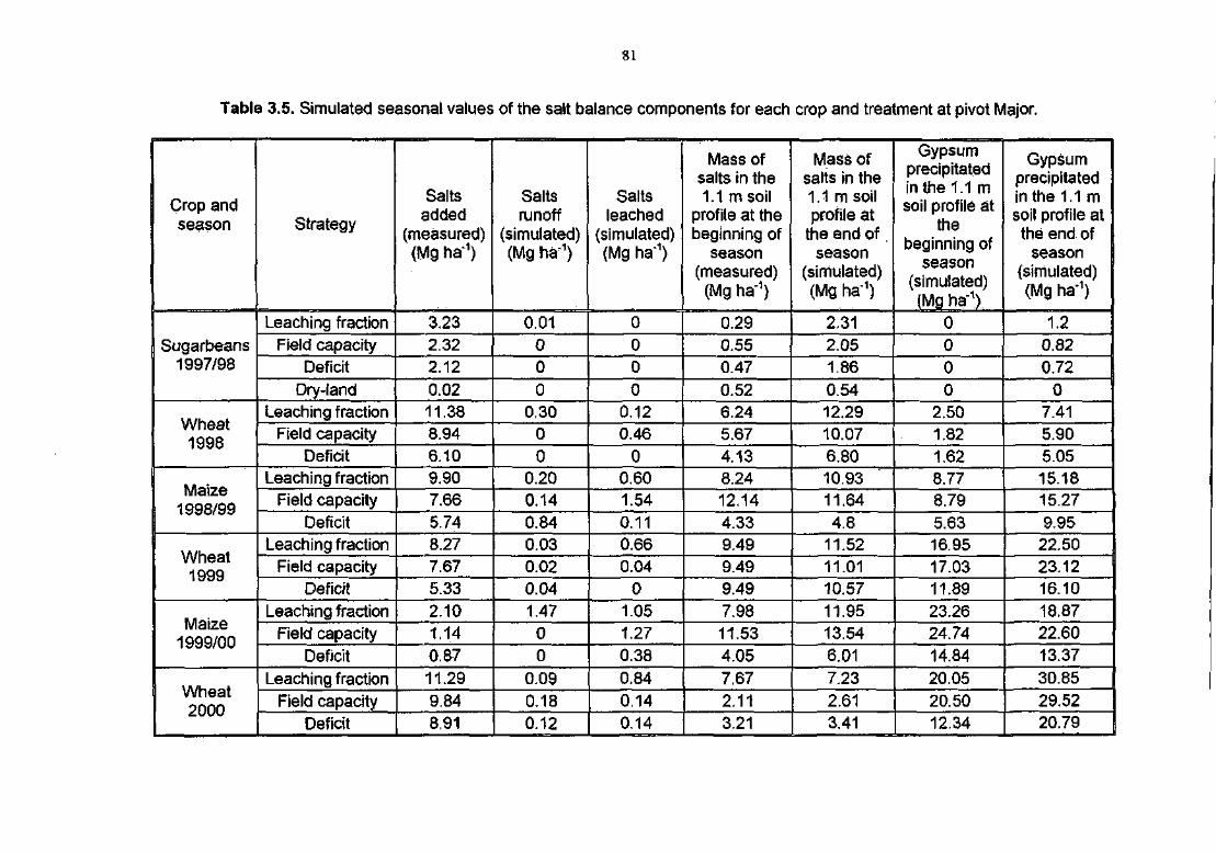
81

Table 3.5. Simulated seasonal values of the salt balance components for each crop and treatment at pivot Major.

Crop andseason

Sugarbeans1997/98

Wheat1998

Maize1998/99

Wheat1999

Maize1999/00

Wheat2000

Strategy

Leaching fractionField capacity

Deficit

Dry-landLeaching fraction

Field capacityDeficit

Leaching fractionField capacity

DeficitLeaching fraction

Field capacityDeficit

Leaching fractionField capacity

DeficitLeaching fraction

Field capacityDeficit

Saltsadded

(measured)(Mg ha*1)

3.232.322.120.0211.388.946.109.907.665.748.277.675.332.101.140.8711.299.848.91

Saltsrunoff

(simulated)(Mg ha"1)

0.01000

0.3000

0.200.140.840.030.020.041.47

00

0.090.180.12

Saltsleached

(simulated)(Mg ha'1)

0000

0.120.46

00.601.540.110.660.04

01.051.270.380.840.140.14

Mass ofsalts in the1.1 m soil

profile at thebeginning of

season(measured)

(Mg ha'1)

0.290.550.470.526.245.674.138.2412.144.339.499.499.497.9811.534.057.672.113.21

Mass ofsalts in the1.1 m soilprofile at

the end of.season

(simulated)(Mg ha1)

2.312.051.860.5412.2910.076.8010.9311.644.8

11.5211.0110.5711.9513.546.017.232.613.41

Gypsumprecipitatedin the 1.1 msoil profile at

thebeginning of

season(simulated)(Mg ha"1)

0000

2.501.821.628.778.795.6316.9517.0311.8923.2624.7414.8420.0520.5012.34

Gypsumprecipitatedin the 1.1 msoil profile atthe end of

season(simulated)(Mg ha"1)

1.20.820.72

07.415.905.0515.1815.279.95

22.5023.1216.1018.8722.6013.3730.8529.5220.79

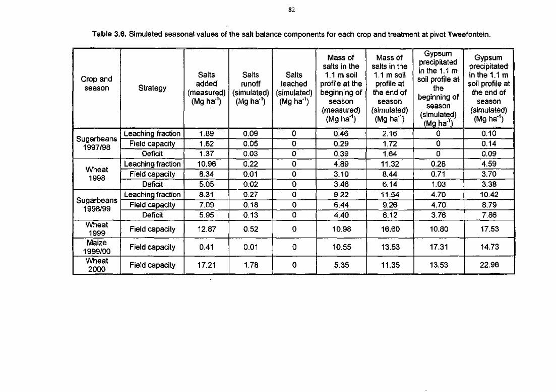
82

Table 3.6. Simulated seasonal values of the salt balance components for each crop and treatment at pivot Tweefontein.

Crop andseason

Sugarbeans1997/98

Wheat1998

Sugarbeans1998/99

Wheat1999Maize

1999/00Wheat2000

Strategy

Leaching fractionField capacity

DeficitLeaching fraction

Field capacityDeficit

Leaching fractionField capacity

Deficit

Field capacity

Field capacity

Field capacity

Saltsadded

(measured)(Mg ha'1)

1.891.621.3710.968.345.058.317.095.95

12.87

0.41

17.21

Saltsrunoff

(simulated)<Mg ha'1)

0.090.050.030.220.010.020.270.180.13

0.52

0.01

1.78

Saltsleached

(simulated)(Mg ha1)

000

000000

0

0

0

Mass ofsalts in the1.1 m soil

profile at thebeginning of

season(measured)

(Mg ha"1)

0.460.290.394.893.103.469.226.444.40

10.98

10.55

5.35

Mass ofsalts in the1.1 rn soilprofile at

the end ofseason

(simulated)(Mg ha1)

2.161.721.64

11.328.446.1411.549.266.12

16.60

13.53

11.35

Gypsumprecipitatedin the 1.1 msoil profile at

thebeginning of

season(simulated)(Mg ha-1)

000

0.280.711.034.704.703.76

10.80

17.31

13.53

Gypsumprecipitatedin the 1.1 msoil profile atthe end of

season(simulated)(Mg ha'1)

0.100.140.094.593.703.3810.428.797.86

17.53

14.73

22.96

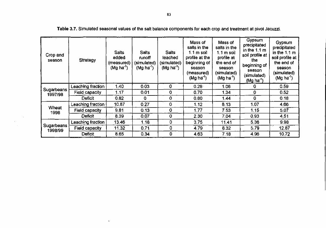
83

Table 3.7. Simulated seasonal values of the salt balance components for each crop and treatment at pivot Jacuzzi.

Crop andseason

Sugarbeans1997/98

Wheat1998

Sugarbeans1998/99

Strategy

Leaching fractionField capacity

DeficitLeaching fraction

Field capacityDeficit

Leaching fractionField capacity

Deficit

Saltsadded

(measured)<Mg ha1)

1.401.170.8210.879.818.3913.4611.328.65

Saltsrunoff

(simulated)(Mg ha1)

0.030.01

0

0.270.130.071.180.710.34

Saltsleached

(simulated)(Mg ha"1)

000000000

Mass ofsalts in the1.1 m soil

profile at thebeginning of

season(measured)

(Mg ha"1)

0.280.700.801.121.772.303.754.794.63

Mass ofsalts in the1.1 msoilprofile at

the end ofseason

(simulated)(Mg ha"1)

1.061.341.448.137.537.0411.418.327.18

Gypsumprecipitatedin the 1.1 msoil profile at

thebeginning of

season(simulated)(Mg ha1)

000

1.071.150.935.365.794.96

Gypsumprecipitatedin the 1.1 msoil profile at

the end ofseason

(simulated)(Mg ha"1)

0.590.520.184.665.074.519.9812.8710.72

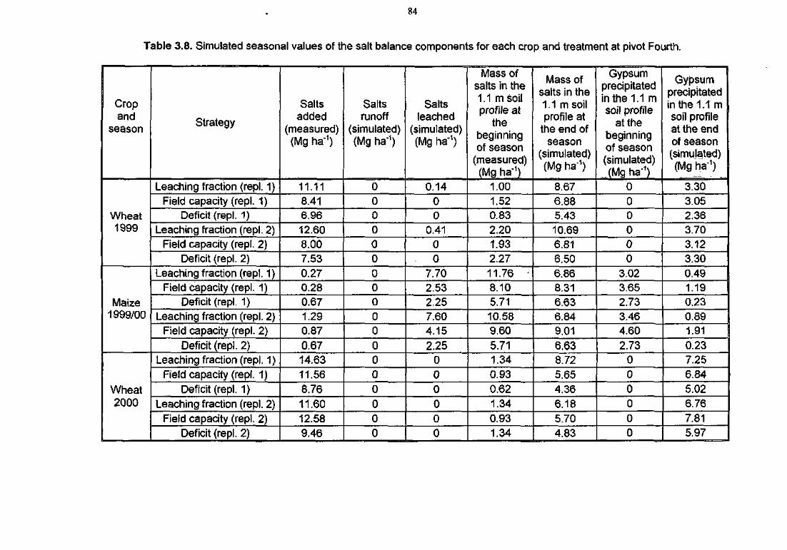
84

Table 3,8. Simulated seasonal values of the salt balance components for each crop and treatment at pivot Fourth.

Cropand

season

Wheat1999

Maize1999/00

Wheat2000

Strategy

Leaching fraction (repl. 1)Field capacity (repl. 1)

Deficit (repl. 1)Leaching fraction (repl. 2)

Field capacity (repl. 2)Deficit (repl. 2)

Leaching fraction (repl. 1)Field capacity (repl. 1)

Deficit (repl. 1)Leaching fraction (repl. 2)

Field capacity (repl. 2)Deficit (repl. 2)

Leaching fraction (repl. 1)Field capacity (repl. 1)

Deficit (repl. 1)Leaching fraction (repl. 2)

Field capacity (repl. 2)Deficit (repl. 2)

Saltsadded

(measured)(Mg ha'1)

11.118.416.9612.608.007.530.270.280.671.290.870.6714.6311.568.7611.6012.589.46

Saltsrunoff

(simulated)(Mg ha'1)

000000000000000000

Saltsleached

(simulated)(Mg ha1)

0.1400

0.410

. 07.702.532.257.604.152.25

000000

Mass ofsalts in the1.1 m soilprofile at

thebeginningof season

(measured)(Mg ha'1)

1.001.520.832.201.932.2711.76 -8.105.7110.589.605.711.340.930.621.340.931.34

Mass ofsalts in the1.1 m soilprofile at

the end ofseason

(simulated)(Mg ha1)

8.676.885.4310.696.816.506.868.316.636.849.016.638.725.654.366.185.704.83

Gypsumprecipitatedin the 1.1 msoil profile

at thebeginningof season(simulated)(Mgha-1)

000000

3.023.652.733.464.602.73

000000

Gypsumprecipitatedin the 1.1 msoil profileat the endof season(simulated)(Mg ha1)

3.303.052.363.703.123.300.491.190.230.891.91

0.237.256.845.026.767.815.97

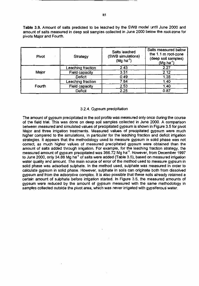
85

Table 3.9. Amount of salts predicted to be leached by the SWB model until June 2000 andamount of salts measured in deep soil samples collected in June 2000 below the root-zone forpivots Major and Fourth.

Pivot

Major

Fourth

Strategy

Leaching fractionField capacity

DeficitLeaching fraction

Field capacityDeficit

Salts leached(SWB simulations)

(Mg ha'1)

2.433.310.497.842.532.25

Salts measured belowthe 1.1 m root-zone(deep soil samples)

(Mg ha"1)2.272.121.351.401.400.87

3.2.4. Gypsum precipitation

The amount of gypsum precipitated in the soil profile was measured only once during the courseof the field trial. This was done on deep soil samples collected in June 2000. A comparisonbetween measured and simulated values of precipitated gypsum is shown in Figure 3.5 for pivotMajor and three irrigation treatments. Measured values of precipitated gypsum were muchhigher compared to the simulations, in particular for the leaching fraction and deficit irrigationstrategies. It appears that the methodology used to measure gypsum in solid phase was notcorrect, as much higher values of measured precipitated gypsum were obtained than theamount of salts added through irrigation. For example, for the leaching fraction strategy, themeasured amount of gypsum precipitated was 366.72 Mg ha-1. However, from December 1997to June 2000, only 34.88 Mg ha'1 of salts were added (Table 3.5), based on measured irrigationwater quality and amount. The main source of error of the method used to measure gypsum insolid phase was adsorbed sulphate. In the method used, sulphate was measured in order tocalculate gypsum in solid phase. However, sulphate in soils can originate both from dissolvedgypsum and from the adsorptive complex. It is also possible that these soils already retained acertain amount of sulphate before irrigation started. In Figure 3.5, the measured amounts ofgypsum were reduced by the amount of gypsum measured with the same methodology insamples collected outside the pivot area, which was never irrigated with gypsiferous water.

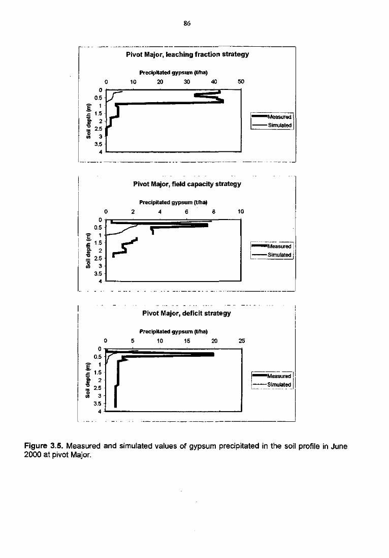
86

Pivot Major, leaching fraction strategy

Precipitated gypsum (t/ha)

Simulated

Pivot Major, field capacity strategy

Precipitated gypsum (t/ha)

2 4 6 8 10

•Measured

-Simulated

Pivot Major, deficit strategy

Precipitated gypsum (t/ha)

5 10 15 20

'Measured

Simulated

Figure 3.5. Measured and simulated values of gypsum precipitated in the soil profile in June2000 at pivot Major.

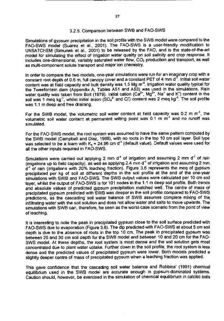
87

3.2.5. Comparison between SWB and FAO-SWS

Simulations of gypsum precipitation in the soil profile with the SWB mode! were compared to theFAO-SWS model (Suarez et al., 2001). The FAO-SWS is a user-friendly modification toUNSATCHEM (Simunek et al., 2001) to be released by the FAO, and is the state-of-the-artmodel for simulating the effect of irrigation water quality on soil salinity and crop response. Itincludes one-dimensional, variably saturated water flow, CO2 production and transport, as wellas multi-component solute transport and major ion chemistry.

In order to compare the two models, one-year simulations were run for an imaginary crop with aconstant root depth of 0.6 m, full canopy cover and a constant PET of 4 mm d'1. Initial soil watercontent was at field capacity and bulk density was 1.5 Mg nrf3. Irrigation water quality typical forthe Tweefontein dam (Appendix A, Tables A51 and A53) was used in the simulations. Rainwater quality was taken from Bolt (1979). Initial cation (Ca2+, Mg2+, Na+ and K+) content in thesoil was 1 meq kg"1, whilst initial anion (SO4

2" and Cl") content was 2 meq kg'1. The soil profilewas 1.1 m deep and free draining.

For the SWB model, the volumetric soil water content at field capacity was 0.2 m m"\ thevolumetric soil water content at permanent wilting point was 0.1 m m"1 and no runoff wassimulated.

For the FAO-SWS model, the root system was assumed to have the same pattern computed bythe SWB model (Campbell and Diaz, 1988), with no roots in the top 10 cm soil layer. Soil typewas selected to be a loam with Ks = 24.96 cm d'1 (default value). Default values were used forall the other inputs required in FAO-SWS,

Simulations were carried out applying 2 mm d"1 of irrigation and assuming 2 mm d*1 of rain(irrigations up to field capacity), as well as applying 2.4 mm d"1 of irrigation and assuming 2 mmd'1 of rain (irrigations with 20% leaching fraction). Figure 3.6 represents the meq of gypsumprecipitated per kg of soil at different depths in the soil profile at the end of the one-yearsimulations with SWB and FAO-SWS. The SWB output values were calculated per 10 cm soillayer, whilst the output of FAO-SWS is for 101 nodes in the 1.1m deep soil profile. Both trendsand absolute values of predicted gypsum precipitation matched well. The centre of mass ofprecipitated gypsum predicted with SWB was deeper in the soil profile compared to FAO-SWSpredictions, as the cascading soil water balance of SWB assumes complete mixing of theinfiltrating water with the soil solution and does not allow water and salts to move upwards. Thesimulations with SWB can, therefore, be seen as the worst-case scenario from the point of viewof leaching.

It is interesting to note the peak in precipitated gypsum close to the soil surface predicted withFAO-SWS due to evaporation (Figure 3.6). The dip predicted with FAO-SWS at about 5 cm soildepth is due to the absence of roots in the top 10 cm. The peak in precipitated gypsum wasbetween 20 and 30 cm soil depth for the SWB mode! and between 10 and 20 cm for the FAO-SWS model. At these depths, the root system is most dense and the soil solution gets mostconcentrated due to plant water uptake. Further down in the soil profile, the root system is lessdense and the predicted values of precipitated gypsum were lower. Both models predicted aslightly deeper centre of mass of precipitated gypsum when a leaching fraction was applied.

This gave confidence that the cascading soil water balance and Robbins' (1991) chemicalequilibrium used in the SWB model are accurate enough in gypsum-dominated systems.Caution should, however, be exercised in the simulation of chemical equilibrium in calcitic soils

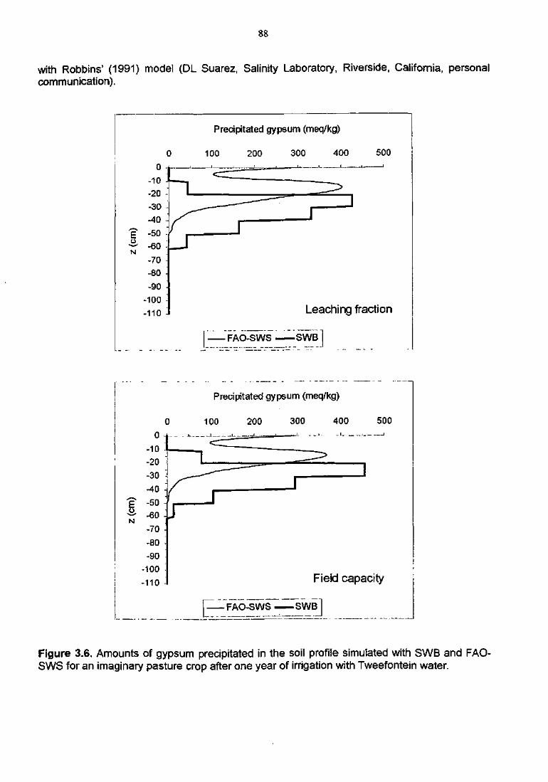
with Robbins' (1991) model (DL Suarez, Salinity Laboratory, Riverside, California, personalcommunication).

o-10 -I

-20 -

-30 -

-40

-50 -

-60

-70

-SO -

-90 •

-100 •

-110

Precipitated gypsum (meq/kg)

100 200 300 400 500

Leaching fraction

. FAO-SWS • SWB

o0

-10-20-30-40-50-60 --70 --80 •

-90-100-110

Precipitated gypsum (meq/kg)

100 200 300 400 500

Field capacity

S WB J

Figure 3.6. Amounts of gypsum precipitated in the soil profile simulated with SWB and FAO-SWS for an imaginary pasture crop after one year of irrigation with Tweefontein water.

89

CHAPTER 4

4. SCENARIO SIMULATIONS

4.1. Introduction

The validation of SWB presented in the previous Sections gave confidence that the model couldbe used for long-term scenario simulations in order to recommend the most suitablemanagement practices.

Different cropping practices have different implications for water utilization, capital outlay, saltprecipitation, and economic impacts. The managers are therefore faced with a decision-makingproblem defined by Massam (1988) as "Given a set of alternate plans, each characterized by aset of assessments for selected criteria, and a set of interest groups whose opinions regardingthe selection of criteria and the assessment have to be considered, provide an appropriateprocedure to define the attractiveness of the alternate plans with a view to identifying the bestone." All these factors have to be valued and harmonised to determine an optimal solution forthe problem.'

Although it was assumed that the cropping system is sustainable, it was still very important toverify this. When deciding what cropping system to adopt, it is important to consider not onlywhich system uses the most water or which system precipitates the most salts but also toassess which system is the best economic option for the particular conditions. To do this, theeconomic feasibility of every cropping system must be evaluated before a decision is made.Multiple Criteria Decision-Making (MCDM) is both an approach and a body of techniques toassist people to relate their multiple, non-commensurate and conflicting criteria to optimaldecisions (Bogetoftand Pruzan, 1991).

The objective of this Section was to investigate the long-term effects of different croppingsystems on the volume of water used for irrigation, and the subsequent precipitation of salts inthe profile. MCDM techniques were also used to advise Kleinkopje Collieries management onthe most economical and environmentally sustainable cropping system for irrigation withgypsiferous mine water.

4.2. Materials and methods

4.2.1. Long-term effects of cropping systems and environmental impact

The long-term modelling approach used by Annandale et al. (1999a) showed that irrigation ofagricultural crops with gypsiferous mine water is sustainable and that the soii can act as aneffective salt sink. In this Section, the SWB model has been used to determine the long-term (30years) water use and yields of different cropping systems. The water and salt balance fordifferent crop rotations were simulated. The model required as inputs, soil, weather and cropdata. Soil data for field Major were used as input. The specific plant growth parameters weredetermined in the field trial undertaken at Kleinkopje Colliery under centre pivot irrigation. Long-term weather data were generated for the region using the CLIMGEN weather data generator(Campbell, 1990) and used in the simulations. Water qualities used for both rain and irrigationcan be seen in Table 4.1.

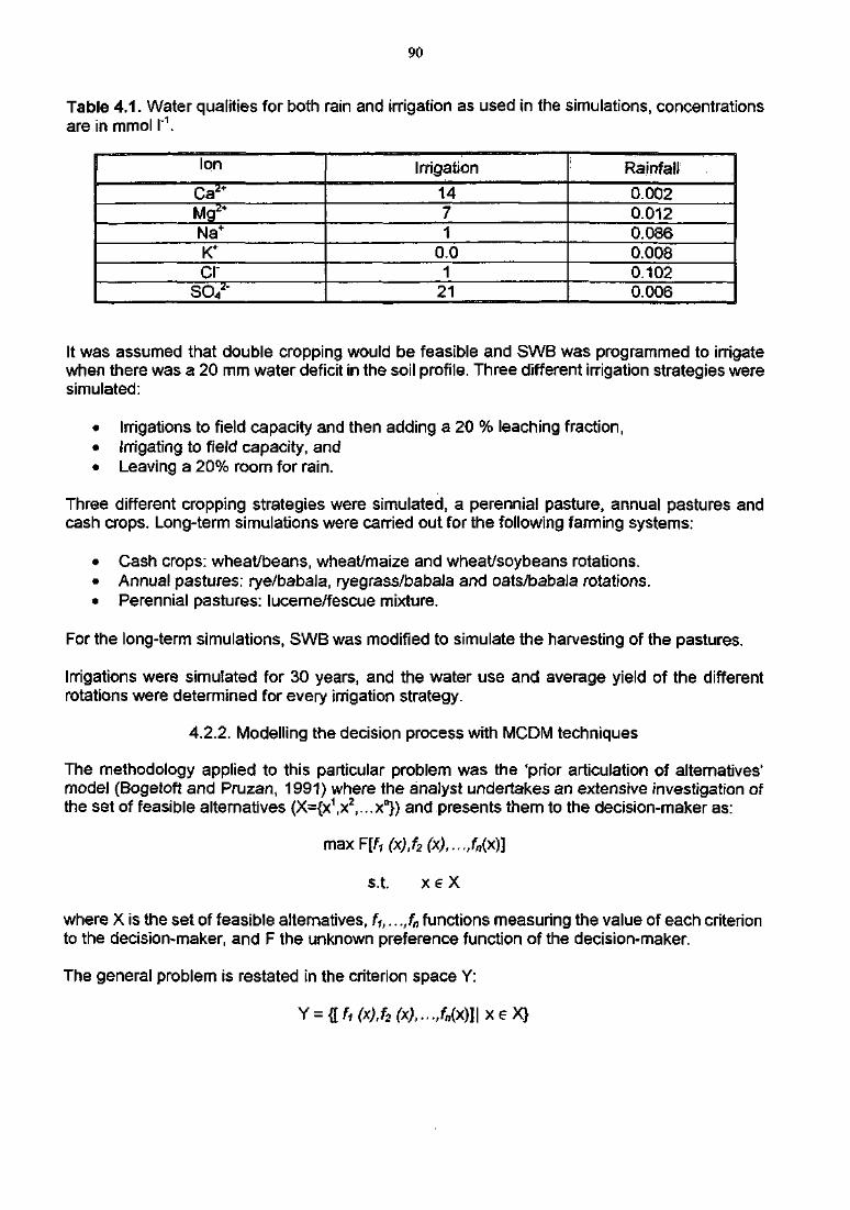
90

Table 4.1. Water qualities for both rain and irrigation as used in the simulations, concentrationsare in mmol I'1.

Ion

Ca2+

M g *Na+

K+

crSO4

2'

Irrigation

1471

0.01

21

: Rainfall

0.0020.0120.0860.0080.1020.006

It was assumed that double cropping would be feasible and SWB was programmed to irrigatewhen there was a 20 mm water deficit in the soil profile. Three different irrigation strategies weresimulated:

• Irrigations to field capacity and then adding a 20 % leaching fraction,• Irrigating to field capacity, and• Leaving a 20% room for rain.

Three different cropping strategies were simulated, a perennial pasture, annual pastures andcash crops. Long-term simulations were carried out for the following farming systems:

• Cash crops: wheat/beans, wheat/maize and wheat/soybeans rotations.• Annual pastures: rye/babala, ryegrass/babala and oats/babala rotations.• Perennial pastures: lucerne/fescue mixture.

For the long-term simulations, SWB was modified to simulate the harvesting of the pastures.

Irrigations were simulated for 30 years, and the water use and average yield of the differentrotations were determined for every irrigation strategy.

4.2.2. Modelling the decision process with MCDM techniques

The methodology applied to this particular problem was the 'prior articulation of alternatives'model (Bogetoft and Pruzan, 1991) where the analyst undertakes an extensive investigation ofthe set of feasible alternatives {X={x1,x2,...x"}) and presents them to the decision-maker as:

maxF[f, (x),f2(x),..Jn(x)]

s.t. x e X

where X is the set of feasible alternatives, f-,,.. .,fn functions measuring the value of each criterionto the decision-maker, and F the unknown preference function of the decision-maker.

The general problem is restated in the criterion space Y:

Y = {[f1(x),f2(x)l..Jn(x)}\xeX}

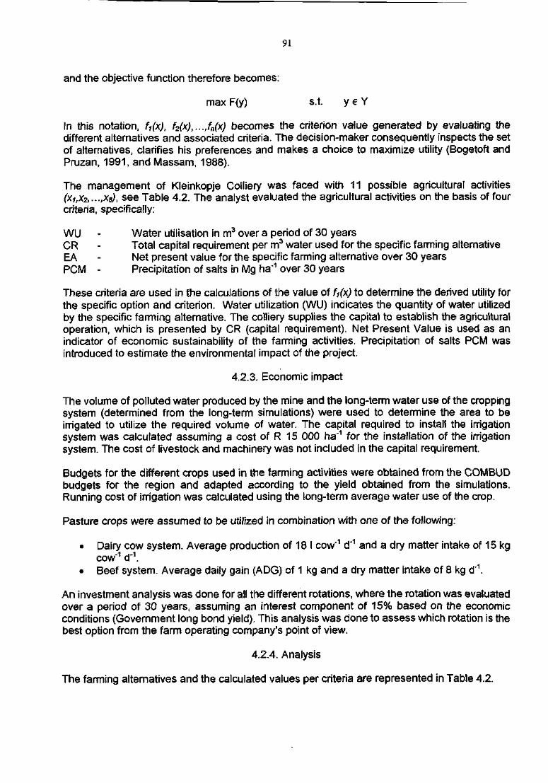
91

and the objective function therefore becomes:

max F(y) s.t. y e Y

In this notation, tyx), f2(x),...,fn(x) becomes the criterion value generated by evaluating thedifferent alternatives and associated criteria. The decision-maker consequently inspects the setof alternatives, clarifies his preferences and makes a choice to maximize utility (Bogetoft andPruzan, 1991, and Massam, 1988).

The management of Kleinkopje Colliery was faced with 11 possible agricultural activities(xi,X2,...,Xs)< s e e Table 4.2. The analyst evaluated the agricultural activities on the basis of fourcriteria, specifically:

WU - Water utilisation in m3 over a period of 30 yearsCR - Total capital requirement per m3 water used for the specific farming alternativeEA - Net present value for the specific farming alternative over 30 yearsPCM - Precipitation of salts in Mg ha"1 over 30 years

These criteria are used in the calculations of the value of U(x) to determine the derived utility forthe specific option and criterion. Water utilization (WU) indicates the quantity of water utilizedby the specific farming alternative. The colliery supplies the capital to establish the agriculturaloperation, which is presented by CR (capital requirement). Net Present Value is used as anindicator of economic sustainabifity of the farming activities. Precipitation of salts PCM wasintroduced to estimate the environmental impact of the project.

4.2.3. Economic impact

The volume of polluted water produced by the mine and the long-term water use of the croppingsystem (determined from the long-term simulations) were used to determine the area to beirrigated to utilize the required volume of water. The capital required to install the irrigationsystem was calculated assuming a cost of R 15 000 ha"1 for the installation of the irrigationsystem. The cost of livestock and machinery was not included in the capital requirement.

Budgets for the different crops used in the farming activities were obtained from the COMBUDbudgets for the region and adapted according to the yield obtained from the simulations.Running cost of irrigation was calculated using the long-term average water use of the crop.

Pasture crops were assumed to be utilized in combination with one of the following:

• Dairy cow system. Average production of 18 I cow'1 d'1 and a dry matter intake of 15 kgcow"1 d"1.

• Beef system. Average daily gain (ADG) of 1 kg and a dry matter intake of 8 kg d"1.

An investment analysts was done for all the different rotations, where the rotation was evaluatedover a period of 30 years, assuming an interest component of 15% based on the economicconditions (Government long bond yield). This analysis was done to assess which rotation is thebest option from the farm operating company's point of view.

4.2.4. Analysis

The farming alternatives and the calculated values per criteria are represented in Table 4.2.

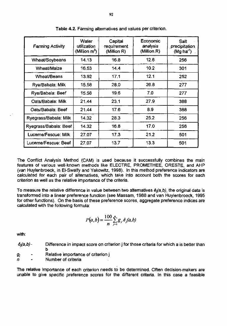
92

Table 4.2. Farming alternatives and values per criterion.

Farming Activity

Wheat/Soybeans

Wheat/Maize

Wheat/Beans

Rye/Babala: Milk

Rye/Babala: Beef

Oats/Babala: Milk

Oats/Babala: Beef

Ryegrass/Babala: Milk

Ryegrass/Babala: Beef

Lucerne/Fescue: Milk

Lucerne/Fescue: Beef

Waterutilization

(Million rn3)

14.13

16.53

13.92

15.58

15.58

21.44

21.44

14.32

14.32

27.07

27.07

Capitalrequirement(Million R)

16.8

14.4

17.1

28.0

me23.1

17.6

28.3

16.8

17.3

13.7

Economicanalysis

(Million R)

12.6

10.2

12.1

26.8

7.0

27.9

8.9

25.2

17.0

21.2

13.3

Saltprecipitation

(Mgha1)

256

301

252

277

277

388

388

256

256

501

501

The Conflict Analysis Method (CAM) is used because it successfully combines the mainfeatures of various well-known methods (ike ELECTRE, PROMETHEE, ORESTE, and AHP(van Huylenbroeck, in El-Swaify and Yakowitz, 1998). In this method preference indicators arecalculated for each pair of alternatives, which take into account both the scores for eachcriterion as well as the relative importance of the criteria.

To measure the relative difference in value between two alternatives e}{a,b), the original data istransformed into a linear preference function (see Massam, 1988 and van Huylenbroeck, 1995for other functions). On the basis of these preference scores, aggregate preference indices arecalculated with the following formula:

with:

9jn

100

n j=\

Difference in impact score on criterion j for those criteria for which a is better thanbRelative importance of criterion jNumber of criteria

The relative importance of each criterion needs to be determined. Often decision-makers areunable to give specific preference scores for the different criteria. In this case a feasible

93

alternative is the Average Value Ranking (AVR) method as discussed in van Huylenbroeck(1990). In this approach the g} factor is calculated with the following formula:

V l

s ,= S —i = k I

where k = the ranking for criterion j (with k = 1 for the most important and k = n for the leastimportant criterion).

The mine management ranked economic impact (EA) as the most important criterion, followedby salt precipitation (PCM), water usage (WU), and capital requirement (CR).

4.3. Results and discussions

The major elements of the water and salt balances, namely total rainfall (R), irrigation (I),evaporation (E), transpiration (T), evapotranspiration (ET), drainage (D), salts added to theprofile, salts leached from the profile and salts precipitated in the profile as simulated over a 30-year period for the three irrigation strategies, are given in Tables 4.3, 4.4 and 4.5.

It is dear that the permanent pasture uses the most water followed by the annual pastures andthen the cash crops. The reason for this is that with a perennial pasture there is a full covercanopy throughout the year and thus transpiration is high, as opposed to cash crops where adrying off period is required during which no irrigation takes place. Annual pastures use morewater than the cash crops because no drying off period is required.

Salts precipitated followed the same trend with the most precipitating under the permanentpasture and the least under the cash crop rotations. The salts that neither leached norprecipitated were those still in the soil solution and those that were intercepted, which wasnegligible.

The Lucerne/Fescue: Milk farming combination is the most preferred farming alternative (seeTable 4.6). Value adding through the use of animal production systems (milk and beef)increases farming profitability. Since farming profitability received the highest ranking from themine management, this is the most important determining factor in the results. Capitalrequirement's low ranking caused a positive bias towards capital intensive farming activities.The reason for the low ranking of the capital requirement criterion is the exorbitant cost of thenext best option to manage environmental pollution, which is reverse osmosis. Therefore, minemanagement gave a higher priority to the economic sustainability of the farming option that ismeasured by the EA or Net Present Value.

The year-round green canopy of the pasture crops increases water usage (WU) and saltprecipitation (PCM). Cash crops require a drying-off period of two to three months during whichno water is required, thus reducing water use. This fact combined with smaller margins in cashcrop alternatives, leads to relatively lower rankings for these traditional irrigation-farmingsystems.

94

Table 4.3. 30-year water and salt balances for the leaching fraction strategy.

Rotation

Lucerne/FescueWheat/Sovbeans2

Wheat/Maize^Wheat/Beans^Rye/Babala3

Ryeqrass/Babala3

Oats/Babala3

R(m)

20.920.920.920.920.920.920.9

I(m)

45.230.522.520.933.236.139.9

E(m.)

15.519.312.512.913.19.811.7

T(m)

30.115.615.814.424.128.630.2

ET(m)

45.634.928.327.337.238.441.9

D(m)

18.015.013.313.014.916.116.5

SaltsAdded

(Mg.ha-1)127185863258893310141120

SaltsLeached(Mgha-1)

741556458439572619622

SaltsPrecipitated

(Mgha"1)493282154130329360422

Table 4.4. 30-year water and salt balances for the field capacity strategy.

Rotation

Lucerne/Fescue1

Wheat/Soybeans2

Wheat/Maize^Wheat/Beans2

Rye/Babalad

Ryegrass/Babala3

Oats/Babala3

R(m)

20.920.920.920.920.920.9

20.9

I(m)

38.525.418.417.427.730.0

33.2

E(m)

10.919.312.012.913.19.7

11.7

T(m)

35.215.616.114.424.128.6

30.2

ET(m)

46.134.928.127.337.238.3

41.9

D(m)

10.49.99.89.59.310.1

9.8

Saltsadded

(Mg ha1)1081716518490111844

933

SaltsLeached(Mg ha'1)

521405348335407440

465

SaltsPrecipitated

(Mg ha'1)517289152136337368

431

Table 4.5. 30-year water and salt balances for the room for rain strategy.

Rotation

Lucerne/Fescue1

Wheat/Soybeans2

Wheat/Maize2

Wheat/Beans2

Rve/Babala^Ryegrass/Babala3

Oats/Babala3

R(m)

20.920.920.920.920.920.9

20.9

I(m)

36.627.118.717.327.429.1

32.6

E(m)

15.721.813.313.613.79.9

12.3

T(m)

30.115.615.814.424.128.6

30.2

ET(m)

45.837.429.128.037.838.5

42.5

D(m)

9.09.08.88.78.38.9

8.5

Saltsadded

(Mg ha*1)1028763526488769819

918

SaltsLeached(Mg ha"1)

477398327317381405

430

SaltsPrecipitated

(Mg ha"1)508340174150349372

444

1 - Perennial pasture2 - Cash crops3 - Annual pasture

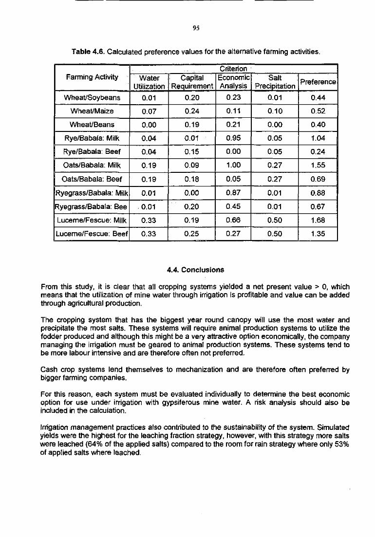
95

Table 4.6. Calculated preference values for the alternative farming activities.

Farming Activity

Wheat/Soybeans

Wheat/Maize

Wheat/Beans

Rye/Babala: Milk

Rye/Babala: Beef

Oats/Babala: Milk

Oats/Babala: Beef

Ryegrass/Babala: Milk

Ryegrass/Babala: Bee

Lucerne/Fescue: Milk

Lucerne/Fescue: Beef

CriterionWater

Utilization

0.01

0.07

0.00

0.04

0.04

0.19

0.19

0.01

0.01

0.33

0.33

• CapitalRequirement

0.20

0.24

0.19

0.01

0.15

0.09

0.18

0.00

0.20

0.19

0.25

EconomicAnalysts

0.23

0.11

0.21

0.95

0.00

1.00

0.05

0.87

0.45

0.66

0.27

SaltPrecipitation

0.01

0.10

0.00

0.05

0.05

0.27

0.27

0.01

0.01

0.50

0.50

Preference

0.44

0.52

0.40

1.04

0.24

1.55

0.69

0.88

0.67

1.68

1.35

4.4. Conclusions

From this study, it is clear that all cropping systems yielded a net present value > 0, whichmeans that the utilization of mine water through irrigation is profitable and value can be addedthrough agricultural production.

The cropping system that has the biggest year round canopy will use the most water andprecipitate the most salts. These systems will require animal production systems to utilize thefodder produced and although this might be a very attractive option economically, the companymanaging the irrigation must be geared to animal production systems. These systems tend tobe more labour intensive and are therefore often not preferred.

Cash crop systems lend themselves to mechanization and are therefore often preferred bybigger farming companies.

For this reason, each system must be evaluated individually to determine the best economicoption for use under irrigation with gypsiferous mine water. A risk analysis should also beincluded in the calculation.

Irrigation management practices also contributed to the sustatnability of the system. Simulatedyields were the highest for the leaching fraction strategy, however, with this strategy more saltswere leached (64% of the applied salts) compared to the room for rain strategy where only 53%of applied salts where leached.

96

A balance between agriculture and environment must be found. This will be a managementpractice that precipitates an acceptable fraction of the applied salts and where yields are stillacceptable to the farming company. It is clear form this study that large quantities of gypsumcan be precipitated in the soil and therefore removed from the water system. However, carefulmanagement of this delicate system is needed to minimize leaching and still achievesatisfactory yields.

97

CHAPTER 5

5. GROUNDWATER MODELLING

In this Chapter of the report, a case study of groundwater modelling is presented for pivotMajor. This modelling study was carried out by the Institute for Groundwater Studies of theUniversity of the Free State using modelled values from the SWB model.

Firstly, the SWB model was run to generate input data for the groundwater model. Thesimulation was run for the period of the field trial (from December 1997 to November 2000)followed by 50 years of scenario simulation. The scenario simulation was done for a shortseason maize-wheat rotation irrigated to field capacity on days when the calculated soilwater deficit was 8 mm (the application rate of pivot Major is 8 mm d'1). Drainage andleaching were assumed from a depth of 3 m (depth at which hard rock was generallyencountered during the deep sampling in June 2000 (Section 2.3.3.1)). The water retentionand chemical properties of the layer below the root-zone (from 1 m to 3 m) were assumed tobe similar to those of the bottom layer of the root-zone (from 0.8 m to 1 m). The generateddata for the groundwater model were:

• Monthly volume of water drained

• Monthly tonnage of salts leached

• Concentrations of the major ionic species expected to be leached (Ca2+, SO42" and

Mg2+) in mg I"1

No significant pollution was detected in the groundwater at pivot Major during the irrigationperiod (Section 2.3.4.3.1). It is, however, expected that pollution will start reporting ifirrigations with mine water continue. A finite element model of the groundwater flow andpotential pollution migration was therefore run for pivot Major assuming a worst-casescenario where groundwater pollution started to occur. This was done to ensure that:

• Monitoring boreholes BH8 and BH9 are placed in localities where they are likely tointercept pollution once it arrives in the groundwater.

• The migration rate and mechanism of water and salt flow along the aquifer aresufficiently understood.

• The modelling capability exists, if required.

A description of the groundwater model and the results for this case study are presented inthe following Sections.

5.1. Model description and scenario modelling

The first step in constructing such a model is the subdivision of the area to be modelled intoelements where the characteristics are similar. Considerations for subdivision of the area aretypically:

• The surface geometry, such as topography, streams, dams and the irrigation area.

• The hydraulic characteristics of the underlying aquifer.

• The potential groundwater quality distribution.

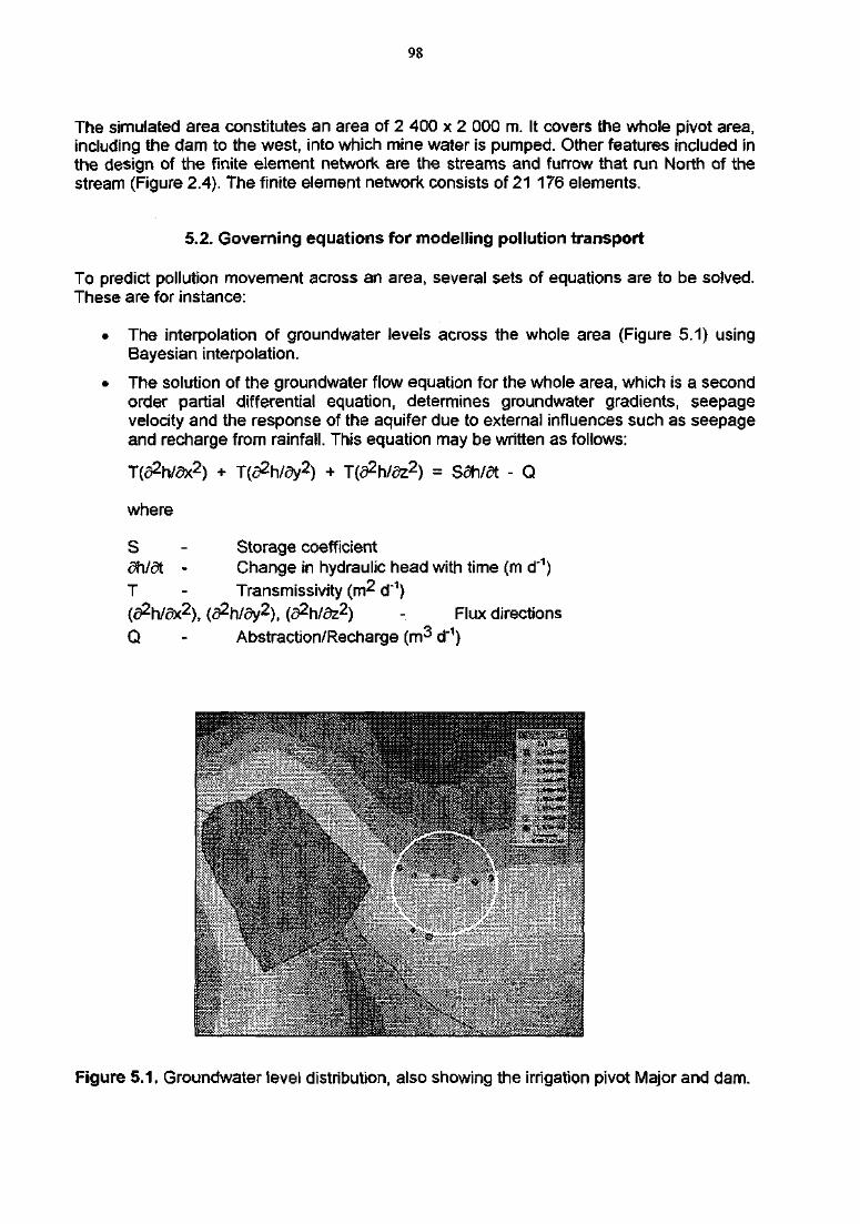
98

The simulated area constitutes an area of 2 400 x 2 000 m. It covers the whole pivot area,including the dam to the west, into which mine water is pumped. Other features included inthe design of the finite element network are the streams and furrow that run North of thestream (Figure 2.4). The finite element network consists of 21 176 elements.

5.2. Governing equations for modelling pollution transport

To predict pollution movement across an area, several sets of equations are to be solved.These are for instance:

• The interpolation of groundwater levels across the whole area (Figure 5.1) usingBayesian interpolation.

• The solution of the groundwater flow equation for the whole area, which is a secondorder partial differential equation, determines groundwater gradients, seepagevelocity and the response of the aquifer due to external influences such as seepageand recharge from rainfall. This equation may be written as follows:

+ T ^ h / o y 2 ) + T ^ h / a z 2 ) = Sah/at - Q

where

Sah/atT

Q

Storage coefficientChange in hydraulic head with time (m d'1)Transmissivity (m2 d~1)

, (a2h/ay2), (cPb/dz2) - Flux directionsAbstraction/Recharge (m3 d'1)

rA-r J-j-J ' ' •> j - s - r - ...I-. - - - - - , . . . \ • :

Figure 5.1. Groundwater level distribution, also showing the irrigation pivot Major and dam.

99

This equation describes the three-dimensional flow of groundwater through substrata,calculating the water table response. The equation may be solved analytically for simpleproblems, though for the irrigation problem, which is more complex, piece-wiseapproximation of the equation is obtained through the finite element method.

Once the water level distribution is available over the whole area, the seepage velocity anddirection can be calculated, using the following equation:

v - k(5h/ai)/n

where

v - Seepage velocity (m d"1)k - Hydraulic conductivity (m d'1)n - Effective porositydh/6\ - Groundwater gradient (m m"1)

On the basis of the hydraulic gradients and flow velocities, the movement of pollutantsthrough the aquifer is calculated next. The mass transport equation is used and is of thefollowing type in its one-dimensional form:

-Vx(5c/ax) = R(5c/at)

where

Dx - Dispersion coefficient in the x-direction (m2 d~1)

c^c/dx2 - Flux directionV x - Seepage velocity (m d'1)

dc/dx. - Change in concentration with distanceR - Retardation coefficientdc/dt - Change in concentration with time (decay)

This equation may be expanded into two or three dimensions, depending on requirements.

It is clear from the above that the coupling of the mass transport equation with the flowequation becomes rather complex because of the additional variables present. Thedispersive properties of the soil and aquifer, degree of convection in these systems, as wellas chemical reactions that take place, must be known before the mass transport equationcan be applied successfully.

Certain simplifying assumptions may be made regarding the problem to be modelled, withoutjeopardizing the value of the model. Examples of assumptions that have been applied forthis modelling exercise are:

• The vertical dimension in the equations may be eliminated by simulating onlypollution movement once it reaches the water table. At the irrigation site, the watertable is within a few metres from the surface ( 1 - 4 m). The vertical dimension forgroundwater flow is therefore very small compared to the lateral dimension, whichfrom the centre of the pivot to the nearest stream is 700 m. After three years ofmonitoring, the pollution plume has not yet arrived in the aquifer below the irrigatedsite. It is assumed, however, that this will happen at some stage in the future. Thetime that it takes for the pollution front to travel through the unsaturated zone should

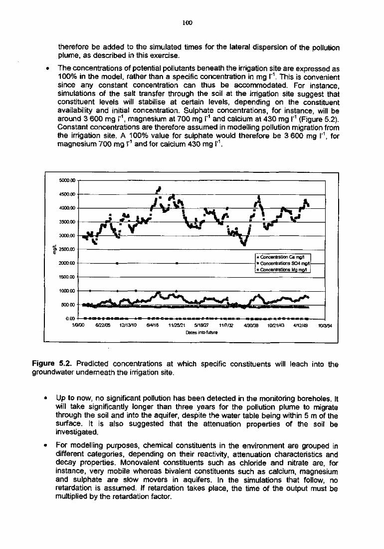
100

therefore be added to the simulated times for the lateral dispersion of the pollutionplume, as described in this exercise.

The concentrations of potential pollutants beneath the irrigation site are expressed as100% in the model, rather than a specific concentration in mg I'1. This is convenientsince any constant concentration can thus be accommodated. For instance,simulations of the salt transfer through the soil at the irrigation site suggest thatconstituent levels will stabilise at certain levels, depending on the constituentavailability and initial concentration. Sulphate concentrations, for instance, will bearound 3 600 mg I"1, magnesium at 700 mg I"1 and calcium at 430 mg I"1 (Figure 5.2).Constant concentrations are therefore assumed in modelling pollution migration fromthe irrigation site, A 100% value for sulphate would therefore be 3 600 mg I"1, formagnesium 700 mg I"1 and for calcium 430 mg I'1.

5000.00

4500.00

4000.00

3500.00

3000.00

2500.00

2000.00

1500.00

1000.00

500.00

0.00

±r

* Concentration Ca mg/l• Concentrations SO4 mg/l« Concentrations Mg mg/l

1/0/00 6/22/05 12/13/10 6/4/16 11/25/21 5/18/27 11/7/32 4/30/38 10/21/43 4/12/49 10/3/54

Dates into future

Figure 5.2. Predicted concentrations at which specific constituents will leach into thegroundwater underneath the irrigation site.

Up to now, no significant pollution has been detected in the monitoring boreholes. Itwill take significantly longer than three years for the pollution plume to migratethrough the soil and into the aquifer, despite the water table being within 5 m of thesurface. It is also suggested that the attenuation properties of the soil beinvestigated.

For modelling purposes, chemical constituents in the environment are grouped indifferent categories, depending on their reactivity, attenuation characteristics anddecay properties. Monovalent constituents such as chloride and nitrate are, forinstance, very mobile whereas bivaient constituents such as calcium, magnesiumand sulphate are slow movers in aquifers. In the simulations that follow, noretardation is assumed. If retardation takes place, the time of the output must bemultiplied by the retardation factor.

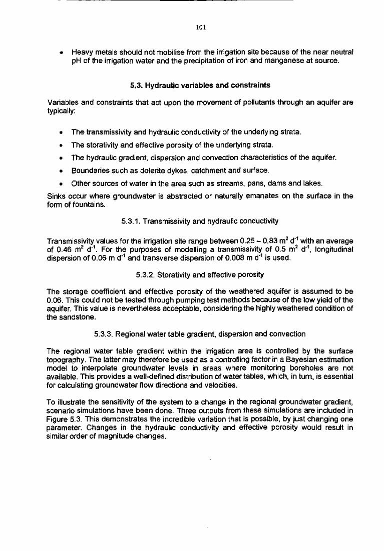
101

• Heavy metals should not mobilise from the irrigation site because of the near neutralpH of the irrigation water and the precipitation of iron and manganese at source.

5.3. Hydraulic variables and constraints

Variables and constraints that act upon the movement of pollutants through an aquifer aretypically:

• The transmissivrty and hydraulic conductivity of the underlying strata.

• The storativity and effective porosity of the underlying strata.

• The hydraulic gradient, dispersion and convection characteristics of the aquifer.

• Boundaries such as dolerite dykes, catchment and surface.

• Other sources of water in the area such as streams, pans, dams and lakes.

Sinks occur where groundwater is abstracted or naturally emanates on the surface in theform of fountains.

5.3.1. Transmissivity and hydraulic conductivity

Transmissivity values for the irrigation site range between 0.25 - 0.83 m2 d'1 with an averageof 0.46 m2 d"1. For the purposes of modelling a transmissivity of 0.5 m2 d"1, longitudinaldispersion of 0.06 m d'1 and transverse dispersion of 0.008 m d'1 is used.

5.3.2. Storativity and effective porosity

The storage coefficient and effective porosity of the weathered aquifer is assumed to be0.06. This could not be tested through pumping test methods because of the low yield of theaquifer. This value is nevertheless acceptable, considering the highly weathered condition ofthe sandstone.

5.3.3. Regional water table gradient, dispersion and convection

The regional water table gradient within the irrigation area is controlled by the surfacetopography. The latter may therefore be used as a controlling factor in a Bayesian estimationmodel to interpolate groundwater levels in areas where monitoring boreholes are notavailable. This provides a well-defined distribution of water tables, which, in turn, is essentialfor calculating groundwater flow directions and velocities.

To illustrate the sensitivity of the system to a change in the regional groundwater gradient,scenario simulations have been done. Three outputs from these simulations are included inFigure 5.3. This demonstrates the incredible variation that is possible, by just changing oneparameter. Changes in the hydraulic conductivity and effective porosity would result insimilar order of magnitude changes.

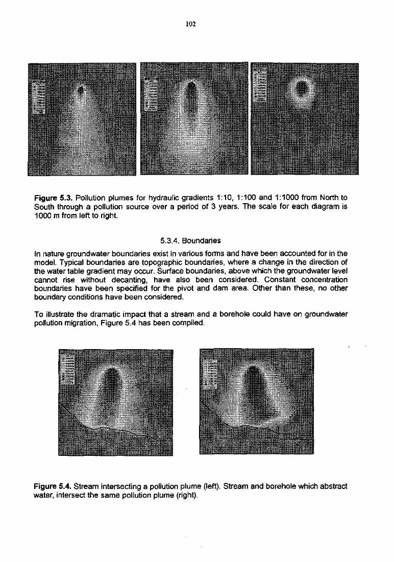
102

Figure 5.3. Pollution plumes for hydraulic gradients 1:10, 1:100 and 1:1000 from North toSouth through a pollution source over a period of 3 years. The scale for each diagram is1000 m from left to right.

5.3.4. BoundariesIn nature groundwater boundaries exist in various forms and have been accounted for in themodel. Typical boundaries are topographic boundaries, where a change in the direction ofthe water table gradient may occur. Surface boundaries, above which the groundwater levelcannot rise without decanting, have also been considered. Constant concentrationboundaries have been specified for the pivot and dam area. Other than these, no otherboundary conditions have been considered.

To illustrate the dramatic impact that a stream and a borehole could have on groundwaterpollution migration, Figure 5.4 has been compiled.

Figure 5.4. Stream intersecting a pollution plume (left). Stream and borehole which abstractwater, intersect the same pollution plume (right).

103

The conclusion is that pollution plumes can be intercepted and managed on condition thatthe flow dynamics is understood. Furthermore, the shape of a pollution plume is dependenton site-specific issues and it is senseless to simulate hypothetical scenarios to demonstratethe variability in possible outcomes. Therefore, the simulations that follow will be based onactual data from the irrigation site.

5.3.5. Sources of water

Sources of water are incorporated in the groundwater model as constant or specified fluxsources. Examples of such sources are the constant water infiltration from the mine waterdam and specified flux from the irrigation pivot area. Another source of water is the rainfallthat recharges the aquifer. Simulations for the water that flows through the soil, done withthe SWB model, suggest that some 20 m3 d"1 passes through the soil and into the aquiferbelow. This is slightly less, but of the same order, as the recharge estimated from the annualfluctuation of water levels in the area, which amounts to 80 m3 d'1.

5.3.6. Sinks

Points where water is taken from the system, such as boreholes, drains or fountains, arereferred to as sinks. Currently, there are no users of groundwater in the area who couldimpact on the movement of pollutants through the aquifer.

5.4. Links between the irrigation and the groundwater model

Flow of irrigation water through the soil has been researched in detail during this project.Below the soil zone lies weathered sandstone. The degree of weathering varies from onelocality to the next in the irrigation area. The conclusion is that a continuum exists in theweathered sandstone, from highly weathered to almost unweathered. In the highlyweathered sandstone, porous flow will be the dominating flow mechanism. Fracture flow willbe the dominant mechanism in the unweathered strata. It should therefore, in theory, takelonger for the irrigation water to pass through the highly weathered sediments than throughthe fractured sediments.

In reality, this does not matter. The vertical distance to the aquifer is less than 4 m. Thehorizontal scale of the pivot is 640 m in diameter. The time that it will take for water to moveunder unity gradient through the 4 m unsaturated zoned would be negligibly small comparedto the time that it would take for the water to flow laterally underneath the pivot. The verticalseepage time can therefore be ignored in groundwater pollution plume modelling.

5.5. Discussion of modelling results

Two simulations have been done. The first simulation was that of potential pollutiondispersion from the irrigation area. The second simulation included the dirty water dam. Theresults from these simulations are included in Figures 5.5 to 5.7.

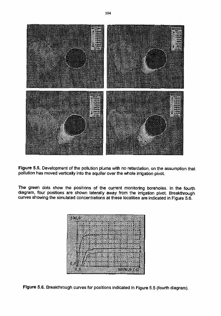
104

I .4

- t .

Figure 5.5. Development of the pollution plume with no retardation, on the assumption thatpollution has moved vertically into the aquifer over the whole irrigation pivot.

The green dots show the positions of the current monitoring boreholes. In the fourthdiagram, four positions are shown laterally away from the irrigation pivot. Breakthroughcurves showing the simulated concentrations at these localities are indicated in Figure 5.6.

+ 1 -

* -

1

nit

+

i

*

,t>*"

• 1 *

1

t

1 t

1 ' ti*4. * 4.• ±

i +

•

I

*i

*t + 4f

•3

1"I

1

m

±

4

• • • • ¥ • + • ^4-

" ; "

f

1 ,

4t

Figure 5.6. Breakthrough curves for positions indicated in Figure 5.5 (fourth diagram).

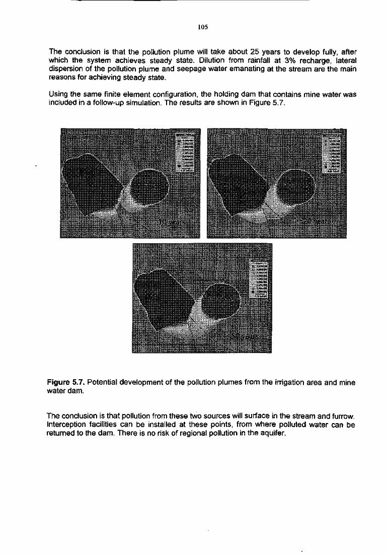
105

The conclusion is that the pollution plume will take about 25 years to develop fully, afterwhich the system achieves steady state. Dilution from rainfall at 3% recharge, lateraldispersion of the pollution plume and seepage water emanating at the stream are the mainreasons for achieving steady state.

Using the same finite element configuration, the holding dam that contains mine water wasincluded in a follow-up simulation. The results are shown in Figure 5.7.

K *

I \ * *I * '

"-J

Figure 5.7. Potential development of the pollution plumes from the irrigation area and minewater dam.

The conclusion is that pollution from these two sources will surface in the stream and furrow.Interception facilities can be installed at these points, from where polluted water can bereturned to the dam. There is no risk of regional pollution in the aquifer.

106

CHAPTER 6

6. CONCLUSIONS AND RECOMMENDATIONS

The conclusions emanating from this research are discussed below, based on the objectivesof the project.

Objective 1

The feasibility of managing irrigation with gypsiferous mine water on a commercial scale insuch a way that surface and groundwater contamination is reduced, while soil suitability andcrop production are maintained, was assessed. In the field trial carried out at KleinkopjeColliery, several crops were successfully irrigated with gypsiferous mine water on acommercial scale. No significant impact on soil, surface and groundwater resources wasobserved, at least in the short-term (three years).

Objective 2

The impact of irrigation with gypsiferous water was evaluated through field monitoring,laboratory experiments and modelling.

Objective 2.1

Yield and plant nutritional effects on a selection of crops that can be grown in the area wereevaluated. Excellent yields were obtained for wheat on both virgin and rehabilitated land,and also short-season maize grown on virgin land. The yields of sugarbeans werereasonable, and definitely higher than those obtained under dry land cropping.

Based on chemical analyses carried out on soil samples collected in the field, exchangeableCa2+ and Mg2+ increased with time, whilst K+ decreased at all four pivot sites. This indicatedthat Ca2+ and, to a certain extent Mg2+, replaced K+ on the cation exchange complex. If lossof K+ through leaching causes nutrient deficiencies to the crop, corrective fertilization shouldbe applied as, or preferably before, symptoms appear. Field monitoring of crop nutrientstatus is therefore essential at this stage of the research and for long-term management withthese water qualities.

In a glasshouse pot trial, calcium and magnesium sulphate salinity decreased the biomassproduction of wheat. This was mainly due to interactions of Mg with the uptake of essentialnutrients. The application of NO3, NH4i and K at rates different from the level consideredbeneficial for non-saline conditions improved wheat growth under sulphate saline conditions.A beneficial effect of higher NH4 supply was observed. This can be ascribed to theantagonistic effect that NH4 exerted on Mg concentrations in plants and/or to a higher N-utilization efficiency where N was supplied as NH4 compared to NO3, which competes foruptake with SO4. Differential application of P had no effect on the yield of wheat. Furtherexperimentation is needed to verify these results under field conditions and determine theoptimal rate, method and timing of especially NH4 when irrigating crops with these calciumand magnesium sulphate enriched waste waters.

The results from the herbicide trial indicated that the Tweefontein and Jacuzzi water mayexert an influence on the adsorption characteristics of atrazine and 2,4-D molecules. This isnot completely unexpected, as one would expect dissolved salts to have an effect on thepolarity of the compounds. This would mean that in the field, there is a possibility that soilretention would decrease and therefore leaching could increase, reducing the efficacy of the

107

herbicides because the herbicide may not stay long enough in the topsoil layer to beabsorbed by plants. Leaching would also lead to groundwater contamination. The increasein activity of atrazine found in bioassays probably does not hold any practical consequencesin terms of herbicide efficacy, selectivity or persistence. In contrast, reduction of metolachloractivity in the presence of gypsum implies that weed control by the herbicide will be poor onsoils irrigated with water containing high levels of calcium sulphate. In the case ofmetolachlor, the finding does not suggest that selectivity of the herbicide towards the cropwould be a concern. The effect on herbicide selectivity is also not an issue in the case of theatrazine, because of the inherent high tolerance of the main crop in which it is used, namelymaize.

In the study on characterization of soil materials, a database of bulk density, water retentionproperties, hydraulic conductivity and solute transport characteristics (dispersion, adsorptionand rate dependant transfers) was generated. Based on these results, it was concluded thathigh bulk density due to soil compaction and the presence of the spoil layer with lowhydraulic conductivity could be limiting factors for crop production under irrigation onrehabilitated land.

Proper preparation of rehabilitated land proved to be important. Settlement on rehabilitatedland caused ponding and waterlogging that had to be overcome by contouring and installingsurface drainage waterways. This problem is related to the physical nature of rehabilitatedland, and not to the chemistry of the water used for irrigation. A spatial variability study and atwo- or three-dimensional model are recommended to accurately predict crop growth andwater use, as well as the water and salt balance under such conditions. In the rehabilitationprocess, if rehabilitated land is to be used for crop production under irrigation, the spoilmaterial should be packed on a slight slope to prevent waterlogging.

Objective 2.2

Several methods for measurement of gypsum precipitated in the soil were considered at theSoil Science Laboratory (University of Pretoria). The Adapted Dilution Method waseventually selected and applied. At the Department of Geology (University of Cape Town),the gypsum saturation index (SI) of a saturated gypsum solution and that of solutions inequilibrium with soil samples to which known masses of gypsum had been added wascalculated using PHREEQC (Parkhurst and Apello, 1999). An attempt to measure gypsumprecipitated in the soil profile was done on deep soil samples collected in June 2000. It was,however, clear from the results obtained that a sufficiently accurate method to measuregypsum precipitation still needs to be developed.

Objective 2.3

The effects of gypsum precipitation and salt accumulation on soil characteristics wereinvestigated in a laboratory trial. There was no evidence that precipitated gypsum affectedthe water retention capacity adversely. Further research is required to confirm these findingsand determine changes in pore size distribution and water retention capacity for largeramounts of gypsum precipitated in the soil.

Objective 2.4

Depth of salinization of soil over time was investigated in the field trial for different irrigationmanagement practices. Soil chemical analyses indicated that soil salinity increasedcompared to the initial conditions. The electrical conductivity of the saturated soil extractincreased mainly due to an increase in concentrations of soluble Ca2+, Mg2+ and SO4

2", whichare the main ionic species in the irrigation water. The values of soil saturated EC were,however, still < 400 mS m'1 even after particularly dry seasons due to gypsum precipitation

108

and leaching of soluble salts. The data generally indicated higher soil salinity in the topsoillayers compared to deeper layers.

Deep soil sampling was carried out in June 2000 in order to explore whether any saltbreakthrough originating from irrigation could be identified deeper in the soil profile. Theresults indicated that, at pivot Major and Tweefontein, most soluble salts were confined tothe upper 1 m, probably due to the presence of the plinthic layer and spoil layers limiting freedrainage. At pivot Fourth, there was a more uniform distribution of salts in the soil profile,with a slight peak between 1.5 and 2 m down in the profile indicating leaching of salts belowthe root-zone.

The results of the spatial variability study indicated that there is a tendency for salinity levelsto be higher in the central region of each pivot. This is believed to be due to the largerquantities of saline irrigation water that have been applied in these zones during the courseof the experiment. The salinity levels measured at the end of the trial are unlikely to have anadverse effect on the growth of most crops.

Objective 2.5

The quality and quantity of drainage water was calculated using the SWB model. Runoffamount and quality data collected at the weirs, indicated that less than 2% of the salts addedsince the beginning of the trial were lost from the irrigated fields through surface andsubsurface runoff from November 1999 to April 2000. More runoff was recorded at pivotTweefontein compared to pivot Major, due to the restricted soil depth and steep slopes of therehabilitated land.

Objective 2.6

Seasonal fluctuations of soil salinity and drainage water characteristics were observed in thefield trial. The results of chemical analyses of soil samples and soil water extracted withceramic cup soil water samplers, indicated that soil salinity is a very dynamic variable as itdepends on many factors, mainly rainfall, irrigation amounts and evapotranspiration. Modelpredictions confirmed that seasonal fluctuations of drainage water characteristics can beexpected. Data collected at the weirs indicated that runoff occurred during the summer rainyseason.

Objective 2.7

The ameliorating effect of gypsiferous water on acidic soils was assessed using results ofchemical analyses on soil samples collected in the field. Soil pH(H2O) generally showed aslight tendency to increase during the course of the trial at all pivots.

Objective 3

The SWB model was developed for predictions of salt and water budgets under irrigationwith gypsum rich mine water.

Objective 4

The SWB model was refined and successfully validated by comparing simulations tomeasurements of crop growth, soil water and salt redistribution obtained in the field trial.This indicated that SWB can be used to predict the water and salt balance in the long term(many decades or centuries). The present version of SWB includes a cascading waterredistribution and assumes complete mixing of irrigation and rainfall with the soil solution.

109

The validation of the chemical equilibrium subroutine in SWB, done by comparing modeloutput to direct measurements of gypsum precipitated in the soil, failed as the method usedto measure precipitated gypsum was inaccurate. The chemical equilibrium model has beenwidely tested by other research groups and is likely to be quite reliable. A reliable gypsumanalysis method is urgently required.

A comparison between SWB and FAO-SWS (Suarez et al., 2001), a modification toUNSATCHEM (Simunek et al., 2001), was run in order to test the chemical equilibriumsubroutine. There was excellent agreement between SWB and FAO-SWS. This gaveconfidence that the cascading soil water balance and Robbins' (1991) chemical equilibriumused in the SWB model are accurate enough in gypsum-dominated systems. Cautionshould, however, be exercised in the simulation of chemical equilibrium in calcitic soils withRobbins' (1991) model (DL Suarez, Salinity Laboratory, Riverside, California, personalcommunication).

Objective 5

Scenario simulations were carried out with SWB in order to recommend the most profitableand environmentally sustainable cropping and irrigation water management system. Fromthis study, it was clear that perennial pastures have the biggest year round green canopy,they will use the most water and precipitate the most salts of all other cropping systemsevaluated. They also require the smallest irrigation area and therefore capital cost to utilizethe water. These systems will require animal production systems to utilize the fodderproduced, and although this might be a very attractive option economically, the companymanaging the irrigation must be geared to animal production systems. These systems tendto be more labour intensive and are therefore often not preferred. Cash crop systems lendthemselves to mechanization and are therefore often preferred by bigger farmingcompanies.

A balance between agriculture and environment must be found. It was clear from thescenario modelling study that large quantities of gypsum can be precipitated in the soil andtherefore removed from the water system. However, careful management of this system isneeded to precipitate a considerable fraction of the applied salts, minimize leaching and stillachieve yields that are acceptable to the farming company. Simulated yields were thehighest for the leaching fraction strategy. However, with this strategy more salts wereleached (64% of the applied salts) compared to the room for rain strategy where only 53% ofapplied salts were leached.

In the scenario modelling study, several management options were proposed for utilization ofgypsiferous mine waste water through irrigation. The acceptability of the proposedmanagement strategies will depend on the standards for environmental protection, as well associal and economic issues. It is essential that strategic decisions are made on croppingsystems, as many options are available, all with different implications for job creation, ease ofmanagement, profitability, capital equipment requirements, water use, irrigated area and saltprecipitation. It is also essential that the necessary management capacity and infrastructure isavailable, as only healthy well-managed crops can use water and precipitate gypsum. Differentcropping systems have different capital and running costs and this should be quantified. It isclear, therefore, that one is dealing with a very flexible system that can be managed in a certainway to achieve the desired result, be it maximum crop production, water use, job creation,economic return or maximum gypsum precipitation and minimum salt leaching.

Objective 6

The SWB model was linked to a groundwater model and provided inputs to associatedgroundwater studies.

110

Objective 7

The groundwater study consisted of monitoring groundwater level and quality from boreholesinstalled on virgin (unmined) land at pivot Major, as well as modelling.

Objective 7.1

Field monitoring indicated that salt migration through soil and aquifers is a slow process.After more than three years of irrigation, there was still no conclusive evidence that salineirrigation water had reached the aquifer below the irrigation site at pivot Major. This is inspite of the fact that groundwater levels are within 1 - 3 m from the surface.

A slight rise in nitrate concentrations was observed at two boreholes. This was derived fromfertilizer application. At five of the boreholes, a small increase in calcium, magnesium andsulphate levels was observed. It is concluded that the system will have to be observed overmany more years before a conclusive answer can be given in terms of the potential long-term impact of irrigation on the aquifer.

Objective 7.2

Output of the SWB model was used as input into the groundwater model in order to predictthe long-term effects of irrigation with gypsiferous mine water on groundwater for a casestudy at pivot Major. Two simulations were done with the groundwater model. The firstsimulation was that of potential pollution dispersion from the irrigation area. The secondsimulation included the dirty water controlled release dam. Modelling of potential pollutionmigration through the aquifer suggested migration to the South-West, eventually to emanatein the stream at a concentration of about 30% of that reaching the aquifer below the irrigatedsite. This drop in salt levels was ascribed to dilution by rainwater infiltration and thedispersive characteristics of the aquifer. The conclusion is that pollution from these twosources (irrigation site and dam) will surface in the stream and furrow. Interception facilitiescan be installed at these points, from where polluted water can be returned to the dam.There is no risk of regional pollution of the aquifer.

The following recommendations for groundwater modelling are made:

• Groundwater quality monitoring should continue for as long as irrigation with minewater continues.

• The monitoring boreholes should be measured with a multi-parameter probe on a bi-annual basis to ensure that sampling is done using the correct method. Samplingshould be done using either stratified or pumping methods, depending on thecircumstances.

• In the event that the monitoring holes are polluted by the bentonite plugs, the holesshould be purged to remove all pollution derived from piezometer installations.

• Parameters that should be analysed for are pH, EC, Ca, Mg, Na, K, Cl, SO4, TAlk,NO3j Fe, Mn and F. In addition, heavy metals should be analysed for, if pH-valuesdrop below 5.0. The samples should be preserved in the field.

• Water levels should be measured in the boreholes before each sampling exercise.

• The data should be added to that generated during this exercise and processed as itbecomes available.

• Anomalies should be identified and followed up.

I l l

• Reports should be issued on an annual basis.

Recommendations for further research

It is recommended to continue the field trial at Kleinkopje in order to collect more years ofdata on the impact of irrigation with gypsiferous mine water on soil and groundwaterresources, as an extremely valuable research site with a well monitored history of irrigationwith such water has been established. Extrapolation to other climatic conditions, soils andwaters is also essential in order to get experience with other conditions. This could beachieved by testing the SWB mode/ for different environmental conditions (water qualities,soils, climates, cropping systems) to extend the scope of the long-term predictive mode ofthe model.

Attention should be paid to groundwater quality, as it will take significantly longer than threeyears for the pollution plume to migrate through the soil and into the aquifer. The linkbetween SWB and the groundwater model gives the opportunity to predict the extent ofgroundwater contamination at specific mines. Groundwater contamination on a regionalscale will depend on the geometry and geological properties of specific sites. It is alsosuggested that the adsorption capacity of the vadose zone be investigated.

The fact that only gypsum can be held up in the soil to some extent, and all other moresoluble salts must be leached for successful crop production, suggests that although thistechnology can make an enormous contribution to water management in the mining industry,it will not be able to completely solve all their problems. Some mines also generatesignificant volumes of saline waters that are not particularly gypsiferous. In order to deal withsuch waters and the concentrated leachate from gypsiferous mine water irrigation, otheragricultural technologies should be considered. The most promising technology is serialbiological concentration, where increasingly concentrated leachate is applied to increasinglysalt tolerant crops to reduce the volumes of water and to allow minima! salt export from themines.

Soil physical analyses of rehabilitated profiles indicated that high bulk density due to soilcompaction and the presence of the spoil layer with low hydraulic conductivity could belimiting factors for crop production under irrigation. It is recommended to investigatemeasures for reducing soil compaction on rehabilitated soil profiles in order to improve landcapability, or make use of this opportunity to create a "duplex" soil from which drainagewater can be retrieved for use in serial biological concentration.

There is opportunity for further improvement to SWB. The simulations with the finite-difference water balance model were carried out without simulating salt redistribution, as theconvection/dispersion subroutine is currently being debugged. The finite-difference modelhas the potential to predict the soil water and salt balance more accurately than thecascading model, once the salt redistribution subroutine becomes operational.

112

CHAPTER 7

REFERENCES

AKOBUNDU 10 (1987) Weed Science in the tropics: Principles and Practices. John Wifey &Sons, New York.

ALASA (1998) Handbook of feeds and plant analysis. D. Palic (ed.).

ALLEN RG, PEREIRA LS, RAES D and SMITH M (1998) Crop evapotranspiration.Guidelines for computing crop water requirements. FAO Irrigation and Drainage Paper No.56. FAO, Rome, Italy.

ANANTHANARAYANA R and HANUMANTHARAJU TH (1992) Interactions of calcium ormagnesium with other plant nutrients. In: Tandon HLS (ed.) Management of nutrientinteractions in agriculture. Fertiliser Development and Consultation Organisation. New Delhi,India.

ANNANDALE JG (1991) Two-dimensional simulation of nitrate leaching in potatoes. PhDThesis, Washington State University, USA, December 1991.

ANNANDALE JG, JOVANOVIC NZ, BENADE N and TANNER PD (1999a) Modelling thelong-term effect of irrigation with gypsiferous water on soil and water resources. Agriculture,Ecosystems and Environment 76 109-119.

ANNANDALE JG, BENADE N, JOVANOVIC NZ, STEYN JM and DU SAUTOY N (1999b)Facilitating irrigation scheduling by means of the soil water balance model. Water ResearchCommission Report No. 753/1/99, Pretoria, South Africa.

ARMSTRONG DE, CHESTERS G and HARRIES RF (1967) Atrazine hydrolysis in soil. SoilSci. Soc. Am. Proc. 31 61-66.

ASHTON FM and CRAFTS AS (1981) Mode of action of herbicides. John Wiley & Sons,New York.

BARNARD RO, RETHMAN NFG, ANNANDALE JG, MENTZ W and JOVANOVIC NZ (1998)The screening of crop, pasture and wetland species for tolerance of polluted wateroriginating in coal mines. Water Research Commission Report No. 582/1/98, Pretoria, SouthAfrica.

BERNSTEIN L, FRANCOIS LE and CLARK RA (1974) Interactive effects of salinity andfertility on yields of grains and vegetables. Agron. J. 66 412-421.

BOGETOFT P and PRUZAN P (1991) Planning with Multiple Criteria: Investigation,Communication, Choice. North-Holland. Amsterdam, Netherlands.

BOLT GH (1979) Soil Chemistry. B. Physico-Chemical Models. Elsevier, New York, 527 pp.

BOTELLA MA, CERDA A, MARTINEZ A and LIPS SH (1994) Nitrate and ammonium uptakeby wheat seedlings as affected by salinity and light. J. of Plant Nutr. 17(5) 839-850.

BOWER CA and HUSS RB (1948) Rapid conductometric method for estimating gypsum insoils. So/7. Sci. 66 199.

113

BRADY NC (1974) The nature and properties of soils. Collier-McMillan, London.

BRESLER E, McNEAL BL and CARTER DL (1982) Saline and Sodic Soils. Springer-Verlag,New York, 236 pp.

BROOKS RH and COREY AT (1964) Hydraulic properties of porous media. Hydrol. PaperNo. 3. Civ. Eng. Dept., Colorado State University, Fort Collins, USA.

BROOKS RH and COREY AT (1966) Properties of porous media affecting fluid flow. J. Irrig.Drain. Div. Am. Soc. Civ. Eng. 92(IR2) 555-560.

BRUCE RR and LUXMORE RJ (1986) Water retention: Field methods. In: Klute A (ed.)Methods of Soil Analysis. Part 1 Physical and Mineralogical Methods. 2nd Edition. AgronomySeries 9 (Part 1), American Society of Agronomy, Soil Science Society of America, Madison,Wisconsin, USA.

CAMPBELL GS (1974) A simple method for determining unsaturated conductivity frommoisture retention data. So/7 Sci. 117 311-314.

CAMPBELL GS (1985) Soil Physics with Basic. Elsevier, Amsterdam, 150 pp.

CAMPBELL GS (1990) CUMGEN, a program that generates weather data (precipitation,maximum and minimum temperature). Unpublished.

CAMPBELL GS and DIAZ R (1988) Simplified soil-water balance models to predict croptranspiration. In: Bidinger FR and Johansen C (Eds.) Drought Research Priorities for theDryland Tropics. ICRISAT, India, 15-26.

CAMPBELL GS and NORMAN JM (1998) An Introduction to Environmental Biophysics.Springer-Verlag, New York. 286 pp.

CAMPBELL GS, FLINT AL, BILSKIE J and CALISSENDORFF C (2001) Calibration andtemperature correction of heat dissipation matric potential sensors. Unpublished.

CAMPBELL RB (2001) The chemical response of deeply leached and weathered soils of theMpumalanga Highveld, South Africa, to irrigation with saline mine water. MSc. Thesis, Dept.of Geology, University of Cape Town.

CAO W and TIBBITS W (1998) Response of potatoes to nitrogen concentrations differ withnitrogen forms. J. of Plant Nutr. 21(4) 615-623.

CLAY Z, SA L, CLAY DE and HARPER SS (1995) Ammonia impact on atrazine leachingthrough undisturbed soil column. J. Environ. Quai. 24 1170-1173.

CLEMENCE BSE (1997) A brief assessment of a weather data generator (CLIMGEN) atSouth African sites. Water SA 23 271-274.

CLOTHIER BE, SCOTTER DR and GREEN AE (1983) Diffusivity and one-dimensionalabsorption experiments. Soil Sci. Soc. Am. J. 47 641-644.

CORDOVILLA MP, OCANA A, LIGERO F and LLUCH C (1995) Growth and macronutrientcontents of faba bean plants: Effects of salinity and nitrate nutrition. J. Plant Nutr. 18(8)1611-1628.

114

DANGARWALA RT (1992) Interactions of iron or manganese with other nutrients. In:Tandon HLS (ed.) Management of nutrient interactions in agriculture. Fertiliser Developmentand Consultation Organisation. New Delhi, India.

DAO TH and L A W LT (1978) Atrazine adsorption on soil as influenced by temperature,moisture content and electrolyte concentration. Weed Sci. 26 390-394.

DE JAGER JM (1994) Accuracy of vegetation evaporation ratio formulae for estimating finalwheat yield. Water SA 20(4) 307-315.

DREVER JM (1997) The Geochemistry of Natural Waters (3rd edition). Prentice-Hall.

DUDLEY LM, WAGENET RJ and JURINAK JJ (1981) Description of soil chemistry duringtransient solute transport. Water Resour. Res. 17(5) 1498-1504.

DU PLESSIS HM (1983) Using lime treated acid mine water for irrigation. Wat. Sci. Tech. 15145-154.

EL-SWAIFY SA and YAKOWITZ DS (1998) Multiple Objective Decision Making for Land,Water, and Environmental Management. Proceedings of the First international Conferenceon Multiple Objective Decision Support Systems (MODSS) for Land, Water, andEnvironmental Management: Concepts, Approaches, and Applications. Lewis Publishers.

FEY MV, TOMLINSON IR and WILLIS JP (1997) Amelioration of acidic soil with an ettringiticby-product of waste water treatment. S. Afr. Jnl. Plant Soil. 14(3) 112-119.

FRENKEL H, GERSTL Z, and RENGER VAN DE VEEN J (1986) Determination of gypsumand cation exchange capacity in arid soils by a resin method. Geoderma 39 67 - 77.

GENSTAT 5 COMMITTEE OF THE STATISTICS DEPARTMENT (1993) Genstat 5 Release3 Reference Manual. lACR-Rothamsted, UK. Clarendon Press: Oxford.

GOMEZ I, NAVARRO PEDRENO J, MORAL R and IBORRA MR (1996) Salinity andnitrogen fertilization affecting the macronutrient content and yield of sweet pepper plants. J.of Plant Nutr. 19{2) 353-359.

GRATTAN SR and GRIEVE CM (1994) Mineral nutrient acquisition and response by plantsgrown in saline environments. In: Pessarakli M (ed.) Handbook of plant and crop stress. NewYork: Marcel Dekker. Review 199, pp. 203-219.

HOAGLAND DR and ARNON Dl (1950) The water culture method for growing plants withoutsoil. University of California, Berkeley; Calif. Agric. Exp. Station Circular 347.

HUANG J and REDMANN RE (1995) Solute adjustment to salinity and calcium supply incultivated and wild barley. J. Plant Nutr. 18(7) 1371-1389.

HURLE KB and FREED VH (1972) Effect of electrolytes on the solubility of some 1, 3, 5 -triazine and substituted urea and their adsorption on soil. Weed Res. 12 1-10.

HUTSON JL and CASS A (1987) A retentivity function for use in soil-water simulationmodels. J. Soil Sci. 38 105-113.

JOHNSTON MA, MEYER JH, SAVAGE MJ and VAN ANTWERPEN R (1994)Electromagnetic induction as a technique for diagnosing and mapping soil salinity.Proceedings of the S.A. Sugar Technologists'Association, 68th Annual Congress, pp. 65-69.

115

JOHNSTON MA, SAVAGE MJ MOOLMAN JH and DU PLESSIS HM (1997) Evaluation ofcalibration methods for interpreting soil salinity from electromagnetic inductionmeasurements. Soil Sci. Soc. Am. J. 61 1627-1633.

JOVANOVIC NZ, BARNARD RO, RETHMAN NFG and ANNANDALE JG (1998) Crops canbe irrigated with lime-treated acid mine drainage. Water SA 24(2) 113-122.

KEREN R and SHAINBERG I (1980) Effect of dissolution rate of industrial and minedgypsum in improving infiltration of a sodic soils. Soil. Sci. Soc. Am. J. 45 103 - 107.

KHAN MG, SILLERBUSH M and LIPS SH (1994) Physiological studies on salinity andnitrogen interactions in alfalfa. I. Biomass production and root development. Journal of PlantNutr. 17(4)657-668.

KLINGMAN GC, ASHTON FM and NOORDHOFF LJ (1982) Weeds Science: Principles andpractices. John Wiiey & Sons, New York.

KLUTE A (1986) Water retention: Laboratory Methods. In: Klute A (ed.) Methods of SoilAnalysis. Part 1 Physical and Mineralogical Methods. 2nd Edition. Agronomy Series 9 (Part1). American Society of Agronomy, Soil Science Society of America, Madison, Wisconsin,USA, 635-662.

LASA B, FRECHILLA S, ALEU M, CONZALEZ-MORO B, LAMSFUS C and APARICIO-TEJP PM (2000) Effects of low and high levels of magnesium on the response of sunflowerplants grown with ammonium and nitrate. Plant Soil. 225 164-174.

LORENTZ SA, NEPFUMBADA MP, ANNANDALE JG and JOVANOVIC NZ (1999) Irrigationwith gypsiferous mine water: soil water dynamics on a rehabilitated profile. Proceedings ofthe 22nd Congress of the Soil Science Society of South Africa, June 1999, Pretoria, SouthAfrica, pp. 152-155.

MAAS EV (1986) Salt tolerance in plants. Appl. Agric. Res. 1(1) 12-26.

MAGALHAES JR and WILCOX GE (1984) Ammonium toxicity development in tomato plantsrelative to nitrogen form and light intensity. J. Plant Nutr. 7(10) 1477-1496.

MAGALHAES JR, MACHADO AT and HUBER DM (1995) Similarities in response of maizeto water logging and ammonium toxicity. J. Plant Nutr. 18(11) 2339-2346.

MARCANO-MARTINEZ E and MCBRIDE MB (1989) Calcium and sulfate retention by twoOxisols of the Brazilian Cerrado. So/7 Sci.Soc.Am.J. 53 63-69.

MASHALI AM (1996) Soil management practices for gypsiferous soils. In: Poch RM (ed.)Proceedings of the International Symposium on Soils with Gypsum. Lleida, 15-21 September1996. Catolinia, Spain.

MASSAM HM (1988) Multi-Criteria Decision-Making (MCDM) Techniques in Planning.Pergamon Press.

MCKENZIE RC, CHOMISTEK W and CLARK NF (1989) Conversion of electromagneticinductance readings to saturated paste extract values in soils for different temperature,texture, and moisture conditions. Can. J. Soil Sci. 69 25-32.

116

MCNEAL BL, OSTER JD and HATCHER JT (1970) Calculation of electrical conductivityfrom solution composition data as an aid to in situ estimation of soil salinity. Soil Sci. 110405-414.

MENGEL K (1976) Effect of potassium on uptake and incorporation of ammonium-nitrogenof rice plants. Plant Soil. 44 547-558.

MENGEL K and KIRKBY EA (1987) Principles of plant nutrition. 4th Revised Edition.International Potash Institute, Bern, Switzerland.

MILLINGTON RJ and QUIRK JP (1961) Permeability of porous solids. Trans. Faraday Soc.57 1200-1207.

MONTEITH JL (1977) Climate and efficiency of crop production in Britain. Philos. Trans. R.Soc. London, Ser. B 281 277-294.

MUALEM Y (1976) A new mode! for predicting the hydraulic conductivity of unsaturatedporous media. Water Resour. Res. 12 513-522.

NELSON RE (1982) Carbonates and gypsum. In: Page AL (ed.) Methods of Soil Analysis,Part 2. Chemical and Microbiological Properties. American Society of Agronomy, Madison,Wisconsin.

NELSON RE, KLAMETH LC and NETTLETON WD (1978) Determining gypsum content andexpressing properties of gypsiferous soils. Soil. Sci. Soc. Am. J. 42 6 5 9 - 6 6 1 .

OSTER JD and RHOADES JD (1975) Calculated drainage water composition and saltburdens resulting from irrigation with river waters in the Western United States. J. Environ.Qual. 4 73-79.

OYONARTE C, ARANA V and ALVARADO (1996) Soil solution and micronutrient availabilityin the rhizosphere of gypsophiles and nongypsophiles plants. In: Poch RM (ed.) InternationalSymposium on Soils with Gypsum. Lleida, 15-21 September 1996.

PANAHI M and ROWELL DL (1996) The effect of gypsum on phosphate sorption incalcareous soils. In: Poch RM (ed.) International Symposium on Soils with Gypsum. Lleida,15-21 September 1996.

PAPADOPOULOS I and REN DIG VV (1983) Interactive effects of salinity and nitrogen ongrowth and yield of tomato plants. Plant Soil 73 47-57.

PARKHURST DL and APPELO CAJ (1999) User's guide to PHREEQC Version 2-Acomputer program for speciation, batch-reaction, one-dimensional transport and inversegeochemical calculations. Water-Resources Investigations Report 99-4259. US GeologicalSurvey, Denver, Colorado.

PULLES W, HOWIE D, OTTO D and EASTON J (1995) A Manual on Mine Water Treatmentand Management in South Africa. Water Research Commission Report No. TT 80/96,Pretoria, South Africa.

PULLES W, HEATH R and HOWARD M (1996) A Manual to Assess and Manage the Impactof Gold Mining Operations on the Surface Water Environment. Water Research CommissionReport No. TT 79/96, Pretoria, South Africa.

117

REUTER DJ (1986) Temperate and sub-tropical crops. In: Reuter DJ and Robinson JB(eds.) Plant analysis. An interpretation manual. Inkata Press. Melbourne, Sydney.

RHOADES JD (1992) Instrumental field methods of salinity appraisal. In: Advances inmeasurement of soil physical properties: bringing theory into practice. Special publication no.30, Soil Sci Soc. Am., Madison, Wis.

RICHARDSON CW and WRIGHT DA (1984) WGEN: A Model for Generating Daily WeatherVariables. US Dept. of Agriculture, Agricultural Research Services.

ROBBINS CH (1991) Solute transport and reactions in salt-affected soils. In: Hanks RJ andRitchie JT (eds.) Modeling plant and soil systems. Agronomy Monograph No. 31, ASA-CSSA-SSSA, Madison, Wisconsin, USA, 365-395.

ROSS PJ (1990) Efficient numerical methods for infiltration using Richard's equation. WaterResour. Res. 26 279-290.

ROSS PJ and BRISTOW KL (1990) Simulating water movement in layered and gradationalsoils using the Kirchhoff transform. Soil Sci. Soc. Am. J. 54 1519-1524.

SHAINBERG I, SUMNER ME, MILLER WP, FARINA MPW, PA VAN MA and FEYMV (1989)Use of gypsum on soils: A review. Adv. Soil Sci. 9 1-111.

SIMUNEK J, SUAREZ DL and SEJNA M (1996) The UNSATCHEM Software Package forSimulating One-Dimensional Variably Saturated Water Flow, Heat Transport, CarbonDioxide Production and Transport, and Solute Transport with Major Ion Equilibrium andKinetic Chemistry, Version 2.0. Research Report No. 141, US Salinity Laboratory, USDA,ARS, Riverside, California. 186 pp.

SIMUNEK J, SUAREZ DL and SEJNA M (2001) UNSATCHEM. Version 2.0. George E.Brown Jr., Salinity Laboratory, USDA-ARS, 450 W. Big Springs Road, Riverside, CA 92507,USA, Compact Disk.

SOIL CLASSIFICATION WORKING GROUP (1991) So/7 Classification. A TaxonomicSystem for South Africa. Dept. of Agricultural Development, Pretoria, South Africa.

STEWART BA, WOOLHISER DA, WISCHMEIER WH, CARO LH and FRERE MH (1976)Control of water pollution from cropland. Vol. 2. An overview. U.S. Department of Agriculture,Agricultural Research Service. Beltsville, Maryland, USA.

SUAREZ DL, VAUGHAN P and LIN J (2001) FAO Soil-Water Salinity. Version 1.2. GeorgeE. Brown Jr., Salinity Laboratory, USDA-ARS, 450 W. Big Springs Road, Riverside, CA92507, USA, Compact Disk.

TANNER CB and SINCLAIR TR (1983) Efficient water use in crop production: research orre-search? In: Taylor HM, Jordan WR and Sinclair TR (eds.) Limitations to Efficient WaterUse in Crop Production. ASA-CSSA-SSSA, 677 S. Segoe Rd., Madison, Wl 53711, 1-27.

TANNER PD, ANNANDALE JG and RETHMAN NFG (1999) Converting problems intoopportunities - The use of gypsiferous mine water for crop irrigation. Proc. 22nd Conf. SoilScience Society of South Africa. Pretoria, South Africa, 160-162.

THOMPSON JG (1980) Acid mine waters in South Africa and their amelioration. Water SA 6130-134.

118

TIMMER VR and STONE EL (1978) Comparative foliar analysis of young balsam fir fertilizedwith nitrogen, phosphorus, potassium and lime. Soil Sci. Am. J. 42 125-130.

TIMMER VR and TENG Y (1999) Foliar nutrient analysis of sugar maple decline:retrospective vector diagnosis. In: Horseley SB and Long RP (eds.) Sugar Maple Ecologyand Health: Proceedings of an International Symposium, June 2-4, 1998, Warren, PA, Gen.Tech. Rep. NE-26. Radnor, PA: U.S. Dept. of Agriculture, Forest Service, NortheasternResearch Station, pp. 69-73.

USDA-SCS (1988) National Engineering Handbook, Hydrology Section 4. U.S. GovernmentPrinting Office, USDA, Washington DC, pp 4-10.

US SALINITY LABORATORY STAFF (1954) Diagnosis and improvement of saline and alkalisoils. USDA Agric. Handbook 60.

US SOIL CONSERVATION SERVICE (1972) Soil survey laboratory methods. Proceduresfor collecting soil samples. Soil survey investigations report no. 1. USDA, U.S. GovernmentPrinting Office, Washington, D.C. 63 p.

VAN GENUCHTEN MTh (1980) A closed-form equation for predicting the hydraulicconductivity of unsaturated soils. Soil Sci. Soc. Am. J. 44 892-898.

VAN GENUCHTEN MTh and NIELSEN DR (1985) On describing and predicting thehydraulic properties of unsaturated soils. Ann. Geophys. 3 615-628.

VAN GENUCHTEN MTh, LEU FJ and LUND LJ (1991) The RETC code for quantifying thehydraulic functions of unsaturated soils. EPA/600/2-91/065, U.S Environmental ProtectionAgency, Ada, OK, USA.

VAN HUYLENBROECK G (1990) Application of Multicriteria Analysis in the EnvironmentalImpact Report for the High Speed Train. Belgian Journal of Operations Research, Statisticsand Computer Science.

VAN HUYLENBROECK G (1995) The Conflict Analysis Method: bridging the gap betweenELECTRE, PROMETEE and ORESTE. European Journal of Operational Research.

VAN STADEN CM (1979) How ERPM uses lime to solve unique underground waterproblem. Coal, Gold and Base Minerals of Southern Africa 27(5) 100-109.

VERBERG K, ROSS PJ and BRISTOW KL (1996) SWIM Version 2 Users Manual. CSIRODivision of Soils, Divisional Report No. 130.

VfLLORA G, PULGAR G, MORENO DA and ROMERO L (1998) Plant nitrogencharacteristics of a semi-salt-tolerant Zucchini variety to sodium chloride treatments. J. ofPlant Nutr. 21 (11) 2343-2355.

WALKER A (1994) Herbicide behaviour in soils in Mediterranean climates. 5m EWRSMediterranean Symposium "Weed control in sustainable agriculture in the Mediterraneanarea", Perugia, Italy.

WEAVER J and REINHARDT CF (1998) Ground water contamination by pesticides. CSIR &University of Pretoria, South Africa.

WILLMOTT CJ (1982) Some comments on the evaluation of model performance. Bull. Am.Met. Soc. 63 1309-1313.

119

ZHAO FJ, WITHERS PJA, EVANS EJ, MONAGHAN J, SALMON SE, SHEWRY PR andMCGRATH SP (1997) Sulphur nutrition: An important factor for the quality of wheat andrapeseed. Soil Sci. Plant Nutr. 43 1137-1142.

120

CHAPTER 8

CAPACITY BUILDING

The capacity building actions carried out during the course of this project were mainlyoriented towards student training.

A large number of students, both from the University of Pretoria and other institutions, havebeen trained on several topics during the course of the project. The students that wereregistered for postgraduate degrees were:

Student

JJB Pretorius

AM van derWesthuizen

MS Mpandeli

1 van der StoepMP Nepfumbada

PHE Strohmenger

L GroblerC de JagerR CampbellG Narciso

DegreeregisteredBScAgric

(Hons)

PhD

M Inst Agr

MScPhD

MSc

MScMScMScMSc

Topic

Economics of croppingsystems

Serial biological concentration

Measuring and modelling soilevaporationTDR systemSoil physics

Plant nutrition

Soil chemistryPlant nutritionSoil chemistry

Remote sensing

Status

Completed inFebruary 2000

To be completed

To be completed

To be completedTo be completed

Completed in March2001

To be completedTo be completedTo be completedTo be completed

Other students were also engaged in the field work during field visits.

The students were trained in the following activities:

They attended several undergraduate and postgraduate courses at the Universityof Pretoria.They were presented with practical work and problems facing two importantbranches of the country's economy (mining and agriculture).They were trained to use instrumentation for field research: principles,installation, management and data manipulation.They were trained in preparing presentations, publications and thesis.

121

CHAPTER 9

TECHNOLOGY TRANSFER

Irrigation with gypsiferous mine water could bring benefits to both the mining industrythrough utilization of polluted water, and to farming communities as an additional watersource for irrigation. This technology could be applied to other mines with similar waterqualities. Due to the encouraging results of this project, the following mines have showninterest in using waste water for irrigation: Syferfontein (Sasol, Secunda), New Vaal (AngloCoal, Sasolburg), Optimum (Ingwe, Hendrina), Kromdraai (Anglo Coal, Witbank), Mpunzi(Witbank) and BCL (Selebi Phikwe, Botswana).

Fanners would also benefit from this technology as all these mines are located in summerrainfall areas, where dry land winter cropping is not feasible.

The experiences gained with irrigation on rehabilitated land should provide generalguidelines as to how the land rehabilitation process should be carried out, especially ifrehabilitated land is to be used for cropping under irrigation.

The results of this project should also provide general guidelines on which cropping systemto choose, and how to manage cropping systems and irrigation water. Cropping system,agronomic practices (fertilization, weed control etc.) and irrigation water management willdepend on the particular environmental conditions (geology, topography, cfimate, type of soiletc.) and water quality.

The SWB model was improved during the course of this project and accurate predictionswere obtained compared to measurements. Scenario simulations can be carried out torecommend the most suitable management practices depending on the specificrequirements of a mine. As this model makes provision for different soils, climates andcrops, it could be used under different environmental conditions. This should, however, betested. SWB, in combination with a groundwater model, could also be used for predictions ofenvironmental pollution for specific case studies.

User-friendly software makes transfer of technology developed in this project relativelysimple. The following computer software was developed during this project:

i) Improved SWB crop growth, soil water and salt balance model.ii) ETo calculator (software for calculation and error analysis of the FAO reference

evapotranspiration).iii) HDS calculator (software for calibration and temperature correction of heat

dissipation soil matric potential sensors),iv) ChemEq model (software for calculation of chemical equilibrium in waters and

soils),v) CLIMGEN (software for generation of weather data).

The following publications and presentations emanated from the research done during thecourse of this project:

Workshops

JOVANOVIC NZ, ANNANDALE JG and BENADE N (1997) Modelling the Long-Term Effectof Irrigation with Gypsiferous Water on Soil and Water Resources. Biological Simulation

122

Forum Workshop, 10 October 1997, SASEX Research Institute, Mount Edgecombe, SouthAfrica.

Conference presentations

JOVANOVIC NZ, ANNANDALE JG and BENADE N (1997) A simple water balance-soilsalinity model for irrigation with gypsiferous water. First All Africa Crop Science Congress,January 1997, Pretoria, South Africa.

ANNANDALE JG, BENADE N, JOVANOVIC NZ and VAN DER WESTHUIZEN AJ (1997)The soil water balance (SWB) irrigation scheduling model. First All Africa Crop ScienceCongress, January 1997, Pretoria, South Africa.

JOVANOVIC NZ and ANNANDALE JG (1998) Modelling crop salt tolerance under differentenvironmental conditions. Joint Congress, Soils and Crops Towards 2000, January 1998,Alpine Heath, KwaZulu-Natal, South Africa.

ANNANDALE JG, BENADE N, JOVANOVIC NZ and DU SAUTOY N (1998) SWB, a userfriendly irrigation scheduling model. Joint Congress, Soils and Crops Towards 2000, January1998, Alpine Heath, KwaZulu-Natal, South Africa.

RETHMAN NFG and JOVANOVIC NZ (1998) Potential forages for areas irrigated withgypsiferous water. 4th International Conference on Land Reclamation, September 1998,Nottingham, United Kingdom.

JOVANOVIC NZ, ANNANDALE JG and PRETORIUS JJB (1999) Modelling and monitoringcrop production, soil properties and drainage water under centre pivot irrigation withgypsiferous mine water. Congress of the SA Society of Crop Production, January 1999,Stellenbosch, South Africa.

PRETORIUS JJB, JOVANOVIC NZ and ANNANDALE JG (1999) Individual calibration ofCampbell Scientific 229 heat dissipation sensors. Congress of the SA Society of CropProduction, January 1999, Stetlenbosch, South Africa.

PRETORIUS JJB, JOVANOVIC NZ, ANNANDALE JG, RETHMAN NFG and KIRSTEN JF(1999) Economic analysis of water use by cropping systems under irrigation with gypsiferousmine water. Congress of the SA Society of Crop Production, January 1999, Stellenbosch,South Africa.

STROHMENGER PHE, CLAASSENS AS, MENTZ WH and BARNARD RO (1999)Interactive effects of sulphate-dominated salinity and fertility in wheat (Triticum aestivum L.).Dahlia Greidinger International Symposium on Nutrient management under salinity andwater stress. 1-4 March 1999. Technion-ITT. Haifa, Israel.

ANNANDALE JG, JOVANOVIC NZ, PRETORIUS JJB and LORENTZ SA (1999)Gypsiferous mine water use in irrigation on rehabilitated open cast mine land: 1) Cropproduction, soil water and salt balance. International Symposium on Ecology of Post-MiningLandscapes, March 1999, Cottbus, Germany.

LORENTZ SA, NEPFUMBADA MP, ANNANDALE JG, JOVANOVIC NZ and ROELOFSE A(1999) Gypsiferous mine water use in irrigation on rehabilitated open cast mine land: 2)Effects of porous media hydraulic properties on water and solute transport. InternationalSymposium on Ecology of Post-Mining Landscapes, March 1999, Cottbus, Germany.

123

JOVANOVIC NZ, ANNANDALE JG, PRETORIUS JJB, LORENTZ SA, RETHMAN NFG andTANNER PD (1999) Gypsiferous mine water use for irrigation: crop production, soil waterand salt balance. 22nd Congress of the Soil Science Society of SA, June 1999, Pretoria,South Africa.

RETHMAN NFG and JOVANOVIC NZ (1999) Potential forages for areas irrigated withgypsiferous water. 22nd Congress of the Soil Science Society of SA, June 1999, Pretoria,South Africa.

PRETORIUS JJB, JOVANOVIC NZ and ANNANDALE JG (1999) Simulated water and saltbalances for cropping systems under irrigation with gypsiferous mine water. 22nd Congressof the Soil Science Society of SA, June 1999, Pretoria, South Africa.

LORENTZ SA, NEPFUMBADA MP, ANNANDALE JG and JOVANOVIC NZ (1999) Irrigationwith gypsiferous mine water: soil water dynamics on a rehabilitated profile. 22nd Congress ofthe Soil Science Society of SA, June 1999, Pretoria, South Africa.

STROHMENGER PHE, CLAASSENS AS, ANNANDALE JG, MENTZ WH and BARNARDRO (1999) Interactive effects of sulphate-dominated salinity and fertility in wheat (Jriticumaestivum L.). 22nd Congress of the Soil Science Society of SA, June 1999, Pretoria, SouthAfrica.

PRETORIUS JJB, DOYER OT, ANNANDALE JG and JOVANOVIC NZ (1999) Managing theenvironmental impact of irrigation with gypsiferous mine water. Agricultural EconomicsAssociation of South Africa Congress, 5-7 October 1999, Club Mykonos, Langebaan, SouthAfrica.

JOVANOVIC NZ, ANNANDALE JG, CLAASSENS AS, LORENTZ SA and TANNER PD(2000) Irrigation with gypsiferous mine water: A case study in Botswana. South AfricanInstitute for Agricultural Engineers 2000 Symposium, July 2000, Hartbeespoort, South Africa.

JOVANOVIC NZ, ANNANDALE JG, CLAASSENS AS, LORENTZ SA and TANNER PD(2001) Irrigation with gypsiferous mine water: A case study in Botswana. SASCP, SAWSS,SSSSA Joint Congress, January 2001, Pretoria, South Africa.

Proceedings

JOVANOVIC NZ, ANNANDALE JG, BENADE N and RETHMAN NFG (1999) SWB - Amechanistic water balance-soil salinity model for irrigation with lime-treated acid minedrainage. Proc. of the 17th Congress on Irrigation and Drainage, 11-19 September 1999,Granada, Spain, Vol. 1G, 73-92.

JOVANOVIC NZ, ANNANDALE JG, TANNER PD and BENADE N (2000) Sustainability ofhigh frequency irrigation with gypsiferous mine water. Proc. of the 6"1 International Micro-Im'gation Congress (Micro 2000), 22-27 October 2000, Cape Town, South Africa.

Peer-reviewed publications

JOVANOVIC NZ and ANNANDALE JG (1997) A laboratory evaluation of Watermarkelectrical resistance and Campbell Scientific 229 heat dissipation matric potential sensors.Water SA 23(3) 227-232.

JOVANOVIC NZ, BARNARD RO, RETHMAN NFG and ANNANDALE JG (1998) Crops canbe irrigated with lime-treated acid mine drainage. Water SA 24(2) 113-122.

124

JOVANOVIC NZ and ANNANDALE JG (1998) Soil and aerial environment affects crop salttolerance - a modelling study. Applied Plant Science 12{2) 39-42.

ANNANDALE JG, JOVANOVIC NZ, BENADE N and TANNER PD (1999) Modelling thelong-term effect of irrigation with gypsiferous water on soil and water resources. Agriculture,Ecosystems and Environment 76 109-119.This paper won the first prize of the Fertilizer Society of South Africa for the best scientificpublication in 1999.

PRETORIUS JJB, DOYER OT, ANNANDALE JG and JOVANOVIC NZ (1999) Managing theenvironmental impact of irrigation with gypsiferous mine water. Agrekon 38(4) 576-584.

ANNANDALE JG, JOVANOVIC NZ, PRETORIUS JJB, LORENTZ SA, RETHMAN NFG andTANNER PD (2001) Gypsiferous mine water use in irrigation on rehabilitated open cast mineland: Crop production, soil water and salt balance. Ecological Engineering 17 153-164.

JOVANOVIC NZ, ANNANDALE JG, CLAASSENS AS, LORENTZ SA and TANNER PD(2001) irrigation with gypsiferous mine water: A case study in Botswana. Mine Waterand theEnvironment 20 65-72.

Dissertations

STROHMENGER PHE (2001) Interactive effects of a calcium and magnesium sulphateenriched waste water on crop growth and nutrition. MSc thesis, University of Pretoria.

CAMPBELL R (2001) The chemical response of deep, leached, and weathered soils of theMpumalanga Highveld, South Africa, to irrigation with saline mine water. MSc thesis,University of Cape Town.

Proposal for archiving data

All data collected and generated in this project will be saved and stored on CD. Copies of theCD will be made available to Mr ME Aken (Anglo Coal Environmental Services, Witbank), MrHC van Zyl (Chamber of Mines), Prof JG Annandale (University of Pretoria, Pretoria) and theWater Research Commission.

APPENDIX A

Tables

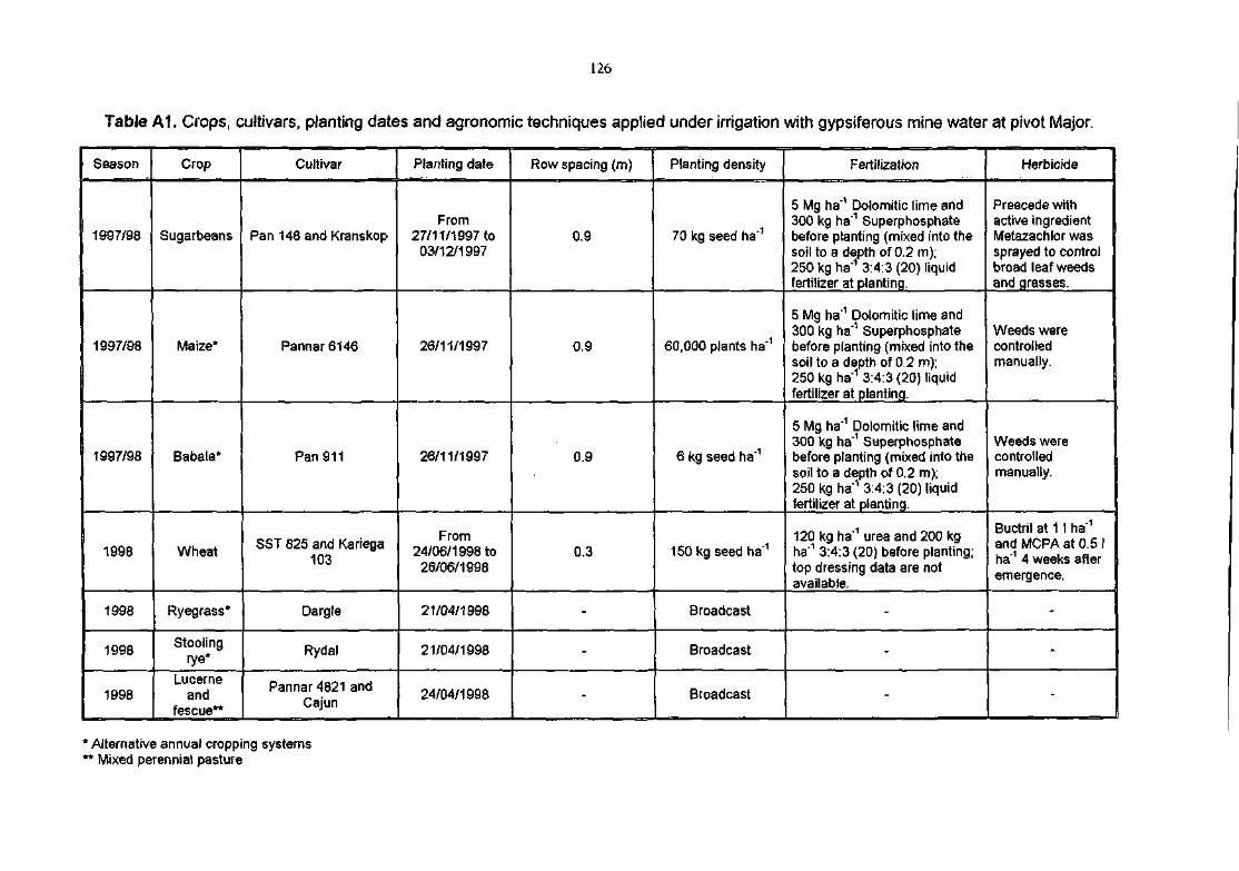
126

Table A1. Crops, cultivars, planting dates and agronomic techniques applied under irrigation with gypsiferous mine water at pivot Major.

Season

1997/98

1997/98

1997/98

1998

1998

1998

1998

Crop

Sugarbeans

Maize*

Babala*

Wheat

Ryegrass*

Stoolingrye*

Lucerneand

fescue**

Cultivar

Pan 148 and Kranskop

Pannar 6146

Pan 911

SST 825 and Kariega103

Dargle

Rydal

Pannar 4821 andCajun

Planting date

From27/11/1997 to

03/12/1997

26/11/1997

26/11/1997

From24/06/1998 to26/06/1998

21/04/1998

21/04/1998

24/04/1998

Row spacing (m)

0.9

0.9

0.9

0.3

-

-

-

Planting density

70 kg seed ha'1

60,000 plants ha"1

6 kg seed ha"1

150 kg seed ha"1

Broadcast

Broadcast

Broadcast

Fertilization

5 Mg ha"1 Dolomitic lime and300 kg ha"1 Superphosphatebefore planting (mixed into thesoil to a depth of 0.2 m);250 kg ha"1 3:4:3 (20) liquidfertilizer at planting.

5 Mg ha'1 Dolomitic lime and300 kg ha'1 Superphosphatebefore planting (mixed into thesoil to a depth of 0.2 m);250 kg ha"1 3:4:3 (20) liquidfertilizer at planting.

5 Mg ha"1 Dolomitic lime and300 kg ha'1 Superphosphatebefore planting (mixed into thesoil to a depth of 0.2 m);250 kg ha'1 3:4:3 (20) liquidfertilizer at planting.

120 kg ha'1 urea and 200 kgha"1 3:4:3 (20) before planting;top dressing data are notavailable.

-

-

-

Herbicide

Preecede withactive ingredientMetazachlor wassprayed to controlbroad leaf weedsand grasses.

Weeds werecontrolledmanually.

Weeds werecontrolledmanually.

Buctril at 1 I ha"1

and MCPA at 0.5 Iha"1 4 weeks afteremergence.

-

-

-

' Alternative annual cropping systems'* Mixed perennial pasture

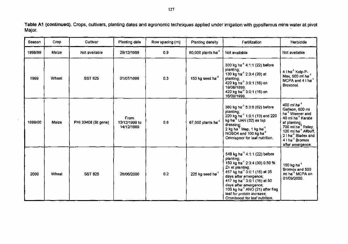
127

Table A1 (continued). Crops, cultivars, planting dates and agronomic techniques applied under irrigation with gypsiferous mine water at pivotMajor.

Season

1998/99

1999

1999/00

2000

Crop

Maize

Wheat

Maize

Wheat

Gultivar

Not available

SST 825

PHI 33408(Bt gene)

SST 825

Planting date

29/12/1998

01/07/1999

From13/12/1999 to

14/12/1999

26/06/2000

Row spacing (m)

0.9

0.3

0.8

0.2

Planting density

60,000 plants ha"1

150 kg seed ha"1

67,500 plants ha"1

225 kg seed ha"1

Fertilization

Not available

300 kg ha"1 4:1:1 (22) beforeplanting;130 kg ha"1 2:3:4 (20) atplanting;420 kg ha"1 3:0:1 (16) on19/08/1999;420 kg ha"1 3:0:1 (16) on16/09/1999.

380 kg ha"1 5:3:6 (02) beforeplanting;220 kg ha"1 1:0:1 (13) and 220kg ha^ UAN (32) as topdressing;2 kg ha^ Map, 1 kg ha"1

NGSO4and 100 kg ha"1

Omnispoor for leaf nutrition.

548 kg ha"1 4:1:1 (22) beforeplanting;150 kg ha"1 2:3:4(30)0.50%Zn at planting;417 kg ha"1 3:0:1 (16) at 35days after emergence;417 kg ha"1 3:0:1 (16) at 50days after emergence;100 kg ha"1 ANO (21) after flagleaf for protein increase;Omniboost for leaf nutrition.

Herbicide

Not available

4 I ha"1 Kelp-P-Max, 500 ml ha"1

MCPA and 4 I ha'1

Broxonol.

400 ml ha"1

Galleon, 600 mlha"1 Wenner and40 ml ha"1 Karateat planting'700 m! ha Relay,120 ml ha"1 Allbuff,21 ha"1 Bladex and4 I ha"1 Bromoxafter emergence.

150 kg ha'1

Bromox and 500ml ha"1 MCPA on01/09/2000.

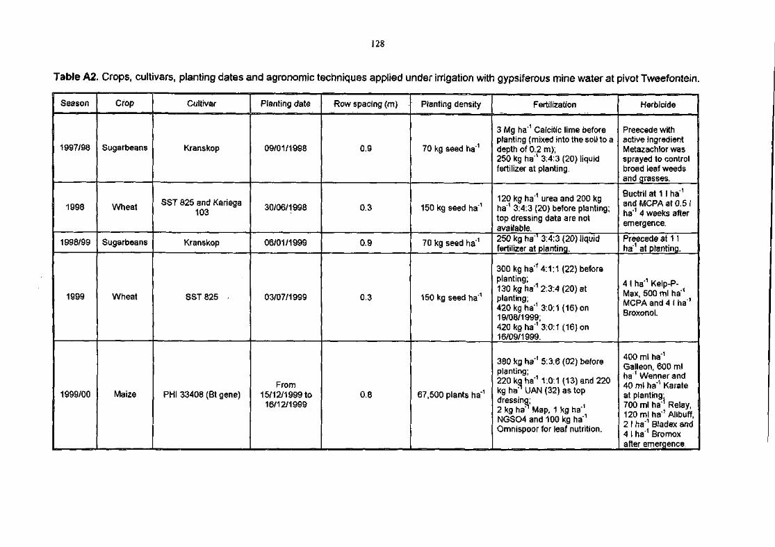
128

Table A2. Crops, cultivars, planting dates and agronomic techniques applied under irrigation with gypsiferous mine water at pivot Tweefontein.

Season

1997/98

1998

1998/99

1999

1999/00

Crop

Sugarbeans

Wheat

Sugarbeans

Wheat

Maize

Cuttivar

Kranskop

SST 825 and Kariega103

Kranskop

SST 825

PHI 33408(Bt gene)

Planting date

09/01/1998

30/06/1998

06/01/1999

03/07/1999

From15/12/1999 to16/12/1999

Row spacing (m)

0.9

0.3

0.9

0.3

0.8

Planting density

70 kg seed ha"1

150 kg seed ha'1

70 kg seed ha'1

150 kg seed ha"1

67,500 plants ha"1

Fertilization

3 Mg ha"1 Calcitic lime beforeplanting (mixed into the soil to adepth of 0.2 m);250 kg ha"1 3:4:3 (20) liquidfertilizer at planting.

120 kg ha"1 urea and 200 kgha"1 3:4:3 (20) before planting;top dressing data are notavailable.250 kg ha"' 3:4:3 (20) liquidfertilizer at planting.

300 kg ha"1 4:1:1 (22) beforeplanting;130 kg ha"1 2:3:4 (20) atplanting;420 kg ha"1 3:0:1 (16) on19/08/1999;420 kg ha"1 3:0:1 (16) on16/09/1999.

380 kg ha"1 5:3:6 (02) beforeplanting;220 kg ha"1 1:0:1 (13) and 220kg ha^ UAN (32) as topdressing;2 kg ha"1 Map, 1 kg ha"1

NGSO4and100kgha"1

Omnispoor for leaf nutrition.

Herbicide

Preecede withactive ingredientMetazachlor wassprayed to controlbroad leaf weedsand grasses.

Buctril at 1 I ha"1

and MCPA at 0.5 1ha"1 4 weeks afteremergence.

Preecede at 1 Iha"1 at planting.

4 1 ha'1 Kelp-P-Max, 500 ml ha"1

MCPA and 4 I ha'1

Broxonol.

400 ml ha"1

Galleon, 600 mlha1 Wenner and40 ml ha"1 Karateat planting-700 ml ha'1 Relay,120 ml ha'1 Allbuff,2 I ha"1 Bladex and4 1 ha"1 Brornoxafter emergence.

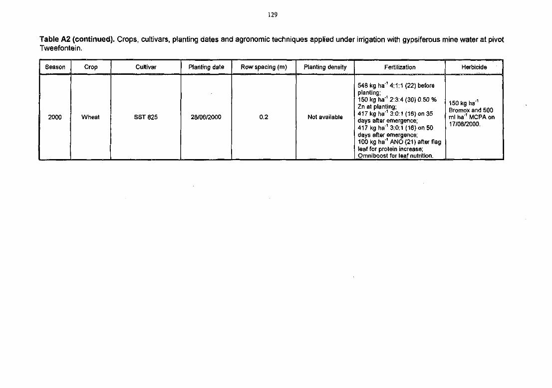
129

Table A2 (continued). Crops, cultivars, planting dates and agronomic techniques applied under irrigation with gypsiferous mine water at pivotTweefontein.

Season

2000

Crop

Wheat

Cultivar

SST 825

Planting date

28/06/2000

Row spacing (m)

0.2

Planting density

Not available

Fertilization

548 kg ha"1 4:1:1 (22) beforeplanting;150 kg ha'1 2:3:4(30)0.50%Zn at planting;417 kg ha'1 3:0:1 (16) on 35days after emergence;417 kg ha'1 3:0:1 (16) on 50days after emergence;100 kg ha"1 ANO (21) after flagleaf for protein increase;Omniboost for leaf nutrition.

Herbicide

150 kg ha"1

Bromox and 500ml ha'1 MCPA on17/08/2000,

130

Table A3. Crops, cultivars, planting dates and agronomic techniques applied under irrigation with gypsiferous mine water at pivot Jacuzzi.

Season

1997/98

1998

1998/99

Crop

Sugarbeans

Wheat

Sugarbeans

Cultivar

Kranskop

SST 825 and Kariega103

Kranskop

Planting date

06/01/1998

30/06/1998

04/01/1999

Row spacing (m)

0.9

0.3

0.9

Planting density

70 kg seed ha'1

150 kg seed ha"1

70 kg seed ha"1

Fertilization

3 Mg ha"1 Calcitic lime beforeplanting (mixed into the soil to adepth of 0,2 m);250 kg ha"1 3:4:3 (20) liquidfertilizer at planting.

120 kg ha"1 urea and 200 kgha"1 3:4:3 (20) before planting.

250 kg ha"1 3:4:3 (20) liquidfertilizer at planting.

Herbicide

Preecede withactive ingredientMetazachlor wassprayed to controlbroad leaf weedsand qrasses.Buctril at 1 I ha1

andMCPAatO.5lha"1 4 weeks afteremerqence.Preecede at 1 Iha'1 at plantinq.

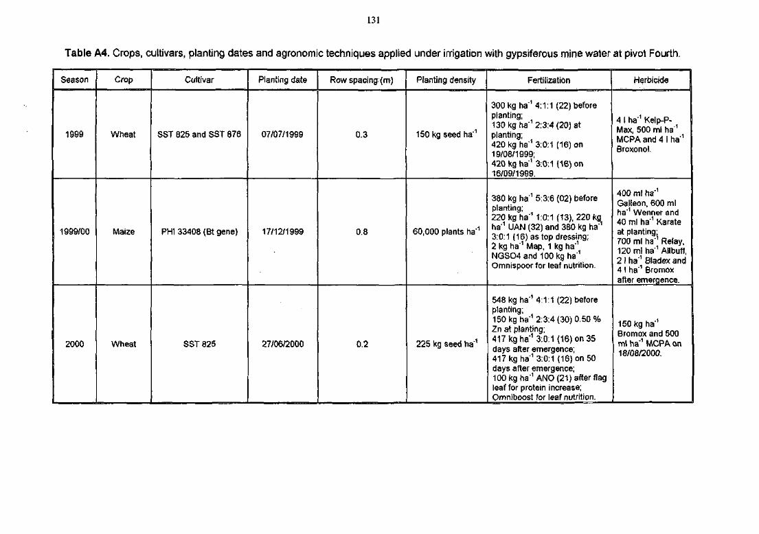
131

Table A4. Crops, cultivars, planting dates and agronomic techniques applied under irrigation with gypsiferous mine water at pivot Fourth.

Season

1999

1999/00

2000

Crop

Wheat

Maize

Wheat

Cultivar

SST 825 and SST 876

PHI 33408(Bt gene)

SST 825

Planting date

07/07/1999

17/12/1999

27/06/2000

Row spacing (m)

0.3

0,8

0.2

Planting density

150 kg seed ha"1

60,000 plants ha'1

225 kg seed ha"1

Fertilization

300 kg ha"1 4:1:1 (22) beforeplanting;130 kg ha"1 2:3:4 (20) atplanting;420 kg ha'1 3:0:1 (16) on19/08/1999;420 kg ha"1 3:0.1 (16) on16/09/1999.

380 kg ha'1 5:3:6 (02) beforeplanting;220 kg ha"' 1:0:1 (13), 220 kgha'1 UAN (32) and 380 kg ha"1

3:0:1 (16) as top dressing;2 kg ha'1 Map, 1 kg ha"1

NGSO4and 100 kg ha"1

Omnispoor for leaf nutrition.

548 kg ha"1 4:1:1 (22) beforeplanting;150 kg ha"1 2:3:4 (30) 0.50%Zn at planting;417 kg ha"1 3:0:1 (16) on 35days after emergence;417 kg ha"1 3:0:1 (16) on 50days after emergence;100 kg ha"1 ANO (21) after flagleaf for protein increase;Omniboost for leaf nutrition.

Herbicide

4 I ha"1 Kelp-P-Max, 500 ml ha"1

MCPA and 4 I ha'1

Broxonol.

400 ml ha"1

Galieon, 600 mlha"1 Wenner and40 ml ha"1 Karateat planting;700 ml ha"1 Relay,120 ml ha"1 Allbuff,21 ha'1 Bladex and4 I ha"1 Bromoxafter emergence.

150 kg ha"1

Bromox and 500ml ha"1 MCPA on18/08/2000.

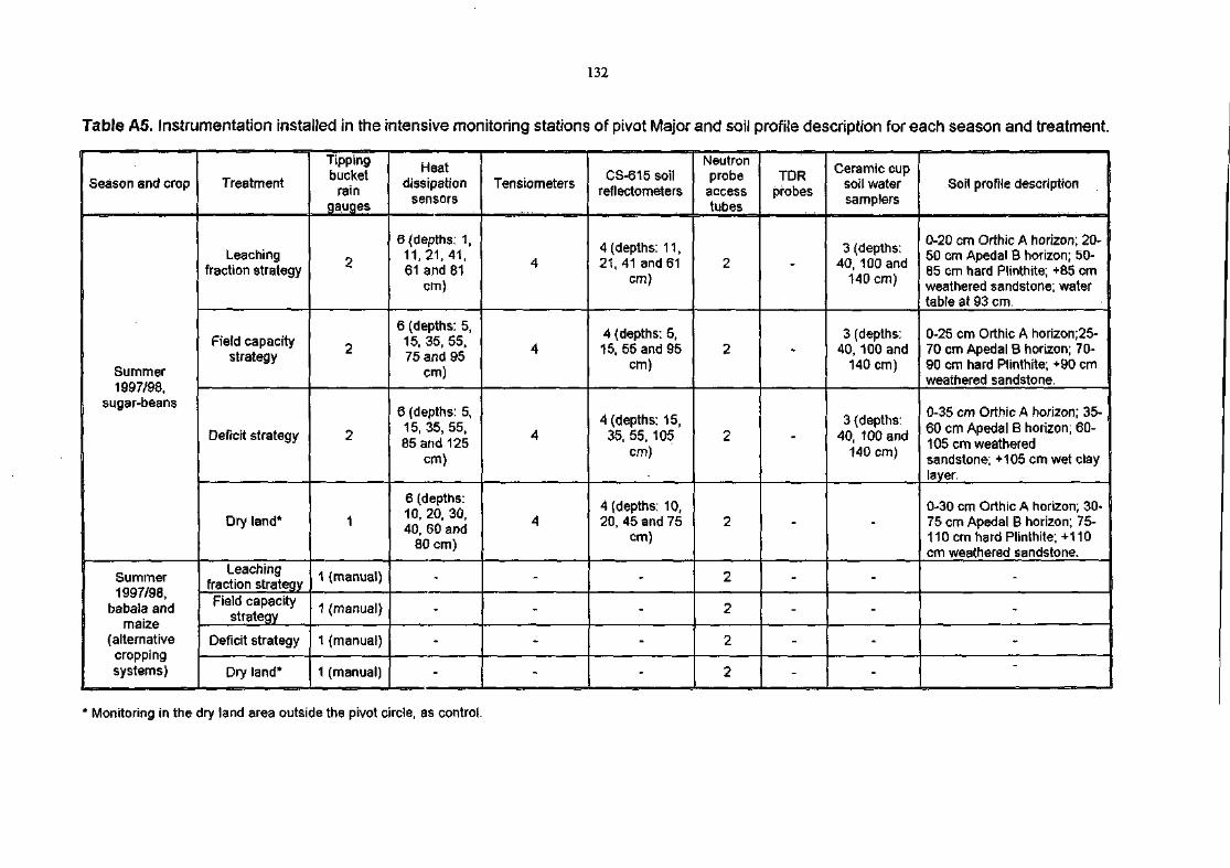
132

Table A5. Instrumentation installed in the intensive monitoring stations of pivot Major and soil profile description for each season and treatment.

Season and crop

Summer1997/98,

sugar-beans

Summer1997/98,

babala andmaize

(alternativecroppingsystems)

Treatment

Leachingfraction strategy

Field capacitystrategy

Deficit strategy

Dry land*

Leachingfraction strategyField capacity

strategy

Deficit strategy

Dry land*

Tippingbucket

raingauges

2

2

2

1

1 (manual)

1 (manual)

1 (manual)

1 (manual)

Heatdissipation

sensors

6 (depths: 1,11,21,41,61 and 81

cm)

6 (depths: 5,15, 35, 55,75 and 95

cm)

6 (depths: 5,15,35,55,85 and 125

cm)

6 (depths:10, 20, 30,40, 60 and

80 cm)

-

-

-

-

Tensiometers

4

4

4

4

-

-

-

-

CS-615 soilreflectometers

4 (depths: 11,21,41 and 61

cm)

4 (depths: 5,15, 55 and 95

cm)

4 (depths: 15,35, 55, 105

cm)

4 (depths: 10,20, 45 and 75

cm)

-

-

-

-

Neutronprobeaccesstubes

2

2

2

2

2

2

2

2

TDRprobes

-

-

-

-

-

-

-

-

Ceramic cupsoil watersamplers

3 (depths:40, 100 and

140 cm)

3 (depths:40, 100 and

140 cm)

3 (depths:40, 100 and

140 cm)

-

-

-

-

-

Soil profile description

0-20 cm Orthic A horizon; 20-50 cm Apedal B horizon; 50-85 cm hard Plinthite; +85 cmweathered sandstone; watertable at 93 cm.

0-25 cm Orthic A horizon;25-70 cm Apedal B horizon; 70-90 cm hard Plinthite; +90 cmweathered sandstone.

0-35 cm Orthic A horizon; 35-60 cm Apedal B horizon; 60-105 cm weatheredsandstone; +105 cm wet claylayer.

0-30 cm Orthic A horizon; 30^75 cm Apedal B horizon; 75-110 cm hard Plinthite;+110cm weathered sandstone.

-

-

-

-

* Monitoring in the dry land area outside the pivot circle, as control.

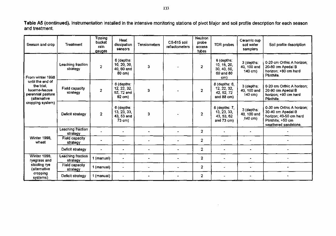
133

Table A5 (continued). Instrumentation installed in the intensive monitoring stations of pivot Major and soil profile description for each seasonand treatment.

Season and crop

From winter 1998until the end of

the trial,lucerne-fescue

perennial pasture(alternative

cropping system)

Winter 1998,wheat

Winter 1998,ryegrass andstooling rye(alternative

croppingsystems)

Treatment

Leaching fractionstrategy

Field capacitystrategy

Deficit strategy

Leaching fractionstrategy

Field capacitystrategy

Deficit strategy

Leaching fractionstrategy

Field capacitystrategy

Deficit strategy

Tippingbucket

raingauges

2

2

2

-

-

-

1 (manual)

1 (manual)

1 (manual)

Heatdissipation

sensors

6 (depths:10, 20, 30,40, 60 and

80 cm)

6 (depths:12, 22, 32,52, 72 and

92 cm)

6 (depths:13,23, 33,43, 53 and

73 cm)

-

-

-

-

-

-

Tensiometers

3

3

3

-

-

-

-

-

-

CS-615 soilreflectometers

-

-

-

-

-

-

-

-

Neutronprobe

accesstubes

2

2

2

2

2

2

2

2

2

TDR probes

8 (depths:10, 15, 20,30, 40, 50,60 and 80

cm)

8 (depths: 6,12, 22, 32,42, 52, 72

and 88 cm)

8 (depths: 7,13,23,33,43, 53, 62and 73 cm)

-

-

-

-

-

-

Ceramic cupsoil watersamplers

3 (depths:40, 10Oand

140 cm)

3 (depths:40, 100 and

140 cm)

3 (depths:40, 100 and

.140 cm)

-

-

-

-

-

-

Soil profile description

0-20 cm Orthic A horizon;20-80 cm Apedal Bhorizon; +80 cm hardPlinthite.

0-20 cm Orthic A horizon;20-90 cm Apedal Bhorizon; +90 cm hardPlinthite.

0-30 cm Orthic A horizon;30-40 cm Apedal Bhorizon; 40-50 cm hardPlinthite; +50 cmweathered sandstone.

-

-

-

-

-

-

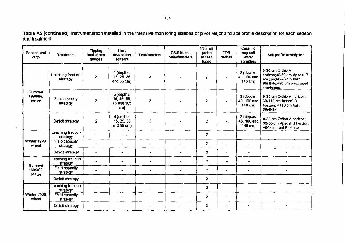
134

Table A5 (continued). Instrumentation installed in the intensive monitoring stations of pivot Major and soil profile description for each seasonand treatment.

Season andcrop

Summer1998/99,

maize

Winter 1999,wheat

Summer1999/00,

Maize

Winter 2000,wheat

Treatment

Leaching fractionstrategy

Field capacitystrategy

Deficit strategy

Leaching fractionstrategy

Field capacitystrategy

Deficit strategy

Leaching fractionstrateqy

Field capacitystrategy

Deficit strategy

Leaching fractionstrategy

Fieid capacitystrategy

Deficit strategy

Tippingbucket rain

gauges

2

2

2

-

-

-

-

-

-

-

-

-

Heatdissipation

sensors

4 (depths:15, 25, 35

and 55 cm)

5 (depths:15, 35,55,75 and 105

cm)

4 (depths:15, 25, 35

and 55 cm)

- •

-

-

-

-

-

-

-

-

Tensiometers

3

3

3

-

-

-

-

-

-

-

-

CS-615soilrefiecto meters

-

-

-

-

-

-

-

-

-

-

-

-

Neutronprobe

accesstubes

2

2

2

2

2

2

2

2

2

2

2

2

TDRprobes

-

- "

-.

-

• -

-

-

-

-

-

-

-

Ceramiccup soilwater

samplers

3 (depths:40, 100 and

140 cm)

3 (depths:40, 100 and

140 cm)

3 (depths,40, 100 and

140 cm)

-

-

-

-

-

-

-

-

-

Soil profile description

0-30 cm Orthic Ahorizon;30-60 cm Apedal Bhorizon;60-90 cm hardPlinthite;+90 cm weatheredsandstone.

0-30 cm Orthic A horizon;30-110 cm Apedal Bhorizon; +110 cm hardPlinthite,

0-30 cm Orthic A horizon;30-60 cm Apedal S horizon;+60 cm hard Plinthite.

-

-

-

-

-

-

-

-

-

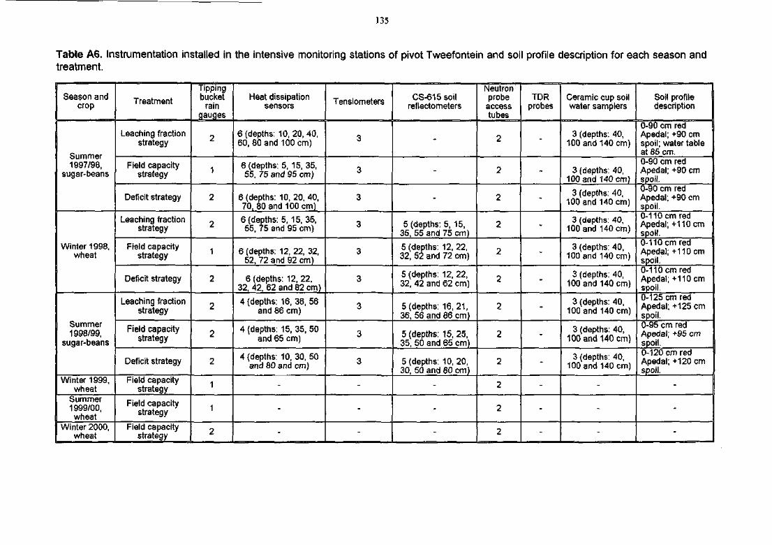
135

Table A6. Instrumentation installed in the intensive monitoring stations of pivot Tweefontein and soil profile description for each season andtreatment.

Season andcrop

Summer1997/98,

sugar-beans

Winter 1998,wheat

Summer1998/99,

sugar-beans

Winter 1999,wheat

Summer1999/00,wheat

Winter 2000,wheat

Treatment

Leaching fractionstrategy

Field capacitystrategy

Deficit strategy

Leaching fractionstrategy

Field capacitystrategy

Deficit strategy

Leaching fractionstrategy

Field capacitystrategy

Deficit strategy

Field capacitystrategy

Field capacitystrategy

Field capacitystrategy

Tippingbucket

raingauges

2

1

2

2

1

2

2

2

2

1

1

2

Heat dissipationsensors

6 {depths: 10,20,40,60, 80 and 100 cm)

6 (depths: 5, 15, 35,55, 75 and 95 cm)

6 (depths: 10, 20, 40,70, 80 and 100 cm)

6 (depths: 5, 15,35,55, 75 and 95 cm)

6 (depths: 12, 22, 32,52, 72 and 92 cm)

6 (depths: 12, 22,32, 42, 62 and 82 cm)

4 (depths: 16, 36, 56and 86 cm)

4 (depths: 15,35,50and 65 cm)

4 (depths: 10,30,50and 80 and cm)

-

-

-

Tensiometers

3

3

3

3

3

3

3

3

3

-

-

-

CS-615 soilreflecto meters

-

-

-

5 (depths: 5, 15,35, 55 and 75 cm)

5 (depths: 12,22,32, 52 and 72 cm)

5 (depths: 12, 22,32, 42 and 62 cm)

5 (depths: 16, 21,36, 56 and 86 cm)

5 (depths: 15,25,35, 50 and 65 cm)

5 (depths: 10,20,30, 50 and 80 cm)

-

-

-

Neutronprobe

accesstubes

2

2

2

2

2

2

2

2

2

2

2

2

TDRprobes

-

-

-

-

-

-

-

-

-

-

-

-

Ceramic cup soilwater samplers

3 (depths: 40,100 and 140 cm)

3 (depths: 40,100 and 140 cm)

3 (depths: 40,100 and 140 cm)

3 (depths: 40,100 and 140 cm)

3 (depths: 40,100 and 140 cm)

3 (depths: 40,100 and 140 cm)

3 (depths: 40,100 and 140 cm)

3 (depths: 40,100 and 140 cm)

3 (depths: 40,100 and 140 cm)

-

-

-

Soil profiledescription

0-90 cm redApedai; +90 cmspoil; water tableat 85 cm.0-90 cm redApedai; +90 cmspoil.0-90 cm redApedai; +90 cmspoil.0-110 cm redApedai; +110 cmspoil.0-110 cm redApedai; +110 cmspoil.0-110 cm redApedai; +110 cmspoil.0-125 cm redApedai; +125 cmspoil.0-95 cm redApedai; +95 cmspoil.0-120 cm redApedal; +120 cmspoil.

-

-

-

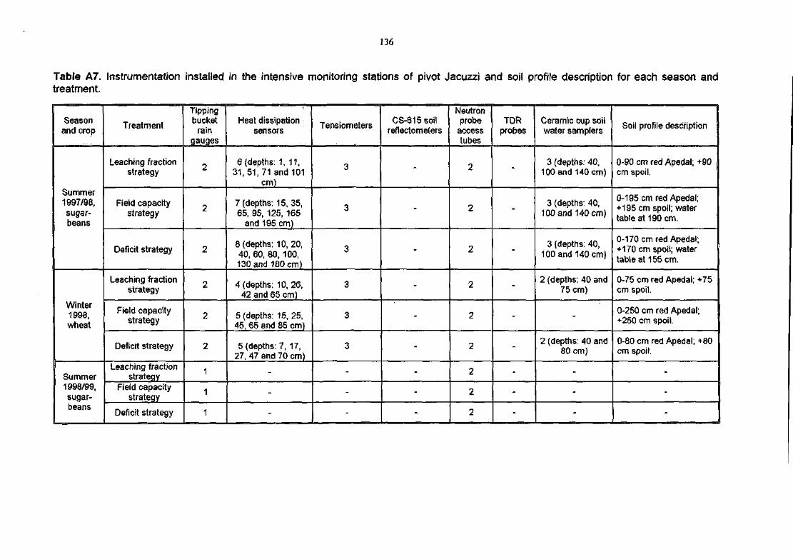
136

Table A7.treatment.

Instrumentation installed in the intensive monitoring stations of pivot Jacuzzi and soil profile description for each season and

Seasonand crop

Summer1997/98,sugar-beans

Winter1998,wheat

Summer1998/99,sugar-beans

Treatment

Leaching fractionstrategy

Field capacitystrategy

Deficit strategy

Leaching fractionstrategy

Field capacitystrategy

Deficit strategy

Leaching fractionstrategy

Field capacitystrategy

Deficit strategy

Tippingbucket

raingauges

2

2

2

2

2

2

1

1

1

Meat dissipationsensors

6 (depths: 1, 11,31,51,71 and 101

cm)

7 (depths: 15, 35,65, 95, 125, 165

and 195 cm)

8 (depths: 10,20,40, 60, 80, 100,130 and 180 cm)

4 (depths: 10,26,42 and 65 cm)

5 (depths: 15,25,45, 65 and 85 cm)

5 (depths: 7, 17,27, 47 and 70 cm)

-

-

-

Tensiometers

3

3

3

3

3

3

-

-

-

CS-615soilreflectometers

-

-

-

-

-

-

-

-

Neutronprobe

accesstubes

2

2

2

2

2

2

2

2

2

TDRprobes

-

-

-

-

-

-

-

-

-

Ceramic cup soilwater samplers

3 (depths: 40,100 and 140 cm)

3 (depths: 40,100 and 140 cm)

3 (depths: 40,100 and 140 cm)

2 (depths: 40 and75 cm)

-

2 (depths: 40 and80 cm)

-

-

-

Soil profile description

0-90 cm red Apedal; +90cm spoil.

0-195 cm red Apedal;+195 cm spoil; watertable at 190 cm.

0-170 cm red Apedal;+170 cm spoil; watertable at 155 cm.

0-75 cm red Apedal; +75cm spoil.

0-250 cm red Apedal;+250 cm spoil.

0-80 cm red Apedal; +80cm spoil.

-

-

-

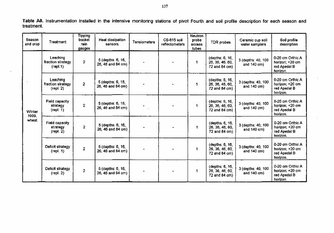
137

Table A8. Instrumentation installed in the intensive monitoring stations of pivot Fourth and soil profile description for each season andtreatment.

Seasonand crop

Winter1999,wheat

Treatment

Leachingfraction strategy

(repl.1)

Leachingfraction strategy

(repl. 2)

Field capacitystrategy(repl.1)

Field capacitystrategy{repl. 2)

Deficit strategy(repl. 1)

Deficit strategy(repl. 2)

Tippingbucket

raingauges

2

2

2

2

2

2

Heat dissipationsensors

5 (depths: 6, 16,26, 46 and 84 cm)

5 (depths: 6, 16,26, 46 and 84 cm)

5 (depths: 6, 16,26, 46 and 84 cm)

5 (depths: 6, 16,26, 46 and 84 cm)

5 (depths: 6, 16,26, 46 and 84 cm)

5 (depths: 6, 16,26, 46 and 84 cm)

Tenstometers

-

-

-

-

-

-

CS-615 soilreflectometers

-

-

-

-

-

-

Neutronprobe

accesstubes

1

1

1

1

1

1

TDR probes

(depths: 6, 16,26, 36, 46, 60,72 and 84 cm)

(depths: 6, 16,26, 36, 46, 60,72 and 84 cm)

(depths: 6, 16,26, 36, 46, 60,72 and 84 cm)

(depths: 6, 16,26, 36, 46, 60,72 and 84 cm)

(depths: 6, 16,26, 36, 46, 60,72 and 84 cm)

(depths: 6, 16,26, 36, 46, 60,72 and 84 cm)

Ceramic cup soilwater samplers

3 (depths: 40, 100and 140 cm)

3 (depths: 40, 100and 140 cm)

3 (depths: 40, 100and 140 cm)

3 (depths: 40, 100and 140 cm)

3 (depths: 40, 100and 140 cm)

3 (depths: 40, 100and 140 cm)

Soil profiledescription

0-20 cm Orthic Ahorizon; +20 cmred Apedal Bhorizon.

0-20 cm Orthic Ahorizon; +20 cmred Apedai Bhorizon.

0-20 cm Orthic Ahorizon; +20 cmred Apedal Bhorizon.

0-20 cm Orthic Ahorizon; +20 cmred Apedal Bhorizon.

0-20 cm Orthic Ahorizon; +20 cmred Apedal Bhorizon.

0-20 cm Orthic Ahorizon; +20 cmred Apedal Bhorizon.

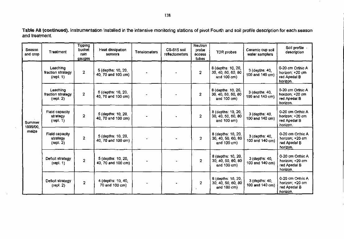
138

Table A8 (continued). Instrumentation installed in the intensive monitoring stations of pivot Fourth and soil profile description for each seasonand treatment.

Seasonand crop

Summer1999/00,

maize

Treatment

Leachingfraction strategy

(repl. 1)

Leachingfraction strategy

(repl. 2)

Field capacitystrategy(repl. 1)

Field capacitystrategy(repl. 2)

Deficit strategy(repl. 1)

Deficit strategy(repl. 2)

Tippingbucket

raingauges

2

2

2

2

2

2

Heat dissipationsensors

5 {depths: 10, 20,40, 70 and 100 cm)

5 (depths: 10,20,40, 70 and 100 cm)

5 (depths: 10,20,40, 70 and 100 cm)

5 (depths: 10,20,40, 70 and 100 cm)

5 (depths: 10,20,40, 70 and 100 cm)

4 (depths: 10, 40,70 and 100 cm)

Tensiometers

-

-

-

-

-

-

CS-615 soilrefleetometers

-

-

-

-

-

-

Neutronprobe

accesstubes

2

2

2

2

2

2

TDR probes

8 (depths: 10, 20,30, 40, 50, 60, 80

and 100 cm)

8 (depths: 10,20,30, 40, 50, 60, 80

and 100 cm)

8 (depths: 10,20,30, 40, 50, 60, 80

and 100 cm)

8 (depths: 10, 20,30, 40, 50, 60, B0

and 100 cm)

8 (depths: 10, 20,30, 40, 50, 60, 80

and 100 cm)

8 (depths: 10, 20,30, 40, 50, 60, 80

and 100 cm)

Ceramic cup soilwater samplers

3 (depths: 40,100 and 140 cm)

3 (depths: 40,100 and 140 cm)

3 (depths: 40,100 and 140 cm)

3 (depths: 40,100 and 140 cm)

3 (depths: 40,100 and 140 cm)

3 (depths: 40,100 and 140 cm)

Soil profile •description

0-20 cm Orthic Ahorizon; +20 cmred Apedal Bhorizon.

0-20 cm Orthic Ahorizon; +20 cmred Apedal Bhorizon.

0-20 cm Orthic Ahorizon; +20 cmred Apedal Bhorizon.

0-20 cm Orthic Ahorizon; +20 cmred Apedal Bhorizon.

0-20 cm Orthic Ahorizon; +20 cmred Apedal Bhorizon.

0-20 cm OrtUic Ahorizon; +20 cmred Apedal Bhorizon.

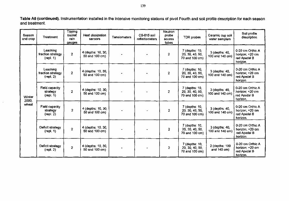
139

Table A8 (continued). Instrumentation installed in the intensive monitoring stations of pivot Fourth and soil profile description for each seasonand treatment.

Seasonand crop

Winter2000,wheat

Treatment

Leachingfraction strategy

(repl. 1)

Leachingfraction strategy

(repl. 2)

Field capacitystrategy(repl. 1)

Field capacitystrategy(repl. 2)

Deficit strategy(repl. 1)

Deficit strategy(repl. 2)

Tippingbucket

raingauges

2

2

2

2

2

2

Heat dissipationsensors

4 (depths: 10,30,50 and 100 cm)

4 (depths: 10,30,50 and 100 cm)

4 (depths: 10,30,50 and 100 cm)

4 (depths: 10, 30,50 and 100 cm)

4 (depths: 10,30,50 and 100 cm)

4 (depths: 10,30,50 and 100 cm)

Tensiometers

-

-

-

-

-

-

CS-615 soilreflecto meters

-

-

-

-

-

-

Neutronprobe

accesstubes

2

2

2

2

2

2

TDR probes

7 (depths: 10,20, 30, 40, 50,70 and 100 cm)

7 (depths: 10,20, 30, 40, 50,70 and 100 cm)

7 (depths: 10,20, 30, 40, 50(

70 and 100 cm)

7 (depths: 10,20, 30, 40, 50,70 and 100 cm)

7 {depths: 10,20, 30, 40, 50,

70 and 100 cm)

7 (depths: 10,20, 30, 40, 50,

70 and 100 cm)

Ceramic cup soilwater samplers

3 (depths: 40,100 and 140 cm)

3 (depths: 40,100 and 140 cm)

3 (depths: 40,100 and 140 cm)

3 (depths: 40,100 and 140 cm)

3 (depths: 40,100 and 140 cm)

2 (depths: 100and 140 cm)

Soil profiledescription

0-20 cm Orthic Ahorizon; +20 cmred Apedal Bhorizon.

0-20 cm Orthic Ahorizon; +20 cmred Apedal Bhorizon.

0-20 cm Orthic Ahorizon; +20 cmred Apedal Bhorizon.

0-20 cm Orthic Ahorizon; +20 cmred Apedal Bhorizon.

0-20 cm Orthic Ahorizon; +20 cmred Apedal Bhorizon.

0-20 cm Orthic Ahorizon; +20 cmred Apedal Bhorizon.

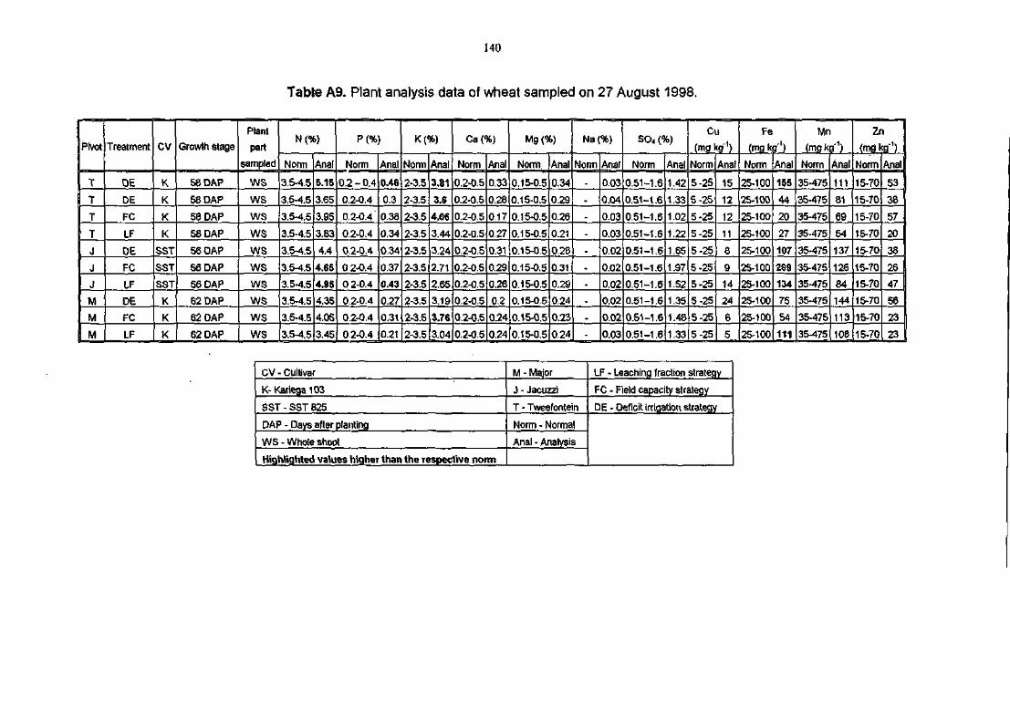
140

Table A9. Plant analysis data of wheat sampled on 27 August 1998.

Pivot

T

T

T

T

J

J

J

M

M

M

Treatment

DE

DE

FC

LF

DE

FC

LF

DE

FC

LF

CV

K

K

K

K

SST

SST

SST

K

K

K

Growth stage

58 DAP

58 DAP

58 DAP

58 DAP

56 DAP

56 DAP

56 DAP

62 DAP

62 DAP

62 DAP

Plant

part

sampled

WS

WS

WS

WS

WS

WS

WS

WS

WS

WS

N(%)

Norm

3.5-4.5

3.5-4.5

3.5-4.5

3.5-4.5

3.5-4.5

3.5-4.5

3.5-4.5

3.5-4.5

3.5-4.5

3.5-4.5

Anal

5.15

3.65

3.95

3.83

4.4

4.65

4.9S

4.35

4.05

3.45

P(%)

Norm

0.2-0.4

0.2-0.4

0.2-0.4

0.2-0.4

0.2-0.4

0 2-0.4

0 2-0.4

02-0.4

0.2-0.4

02-0.4

Anal

0.46

0.3

0.38

0.34

0.34

0.37

0.43

0.27

0.31

0.21

K(%)

Norm

2-3.5

2-3.5

2-3.5

2-3.5

2-3.5

2-3.5

2-3.5

2-3.5

2-3.5

2-3.5

Anal

3.81

3.6

4.06

3.44

3.24

2.71

2.65

31S

3 7R

3.04

Ca{%)

Norm

0.2-0.5

0.2-0.5

0.2-0.5

0.2-0,5

0.2-0.5

0.2-0.5

0.2-0.5

0.2-0.5

0.2-0.5

0.2-0.5

Anal

0,33

0.28

0.17

0.27

0.31

0.29

0.26

0?

n?4

0.24

Mg(%)

Norm

0.15-0.5

0.15-0.5

0.15-0.5

0.15-0.5

0.15-0.5

0.15-0.5

0.15-0.5

0.15-0.5

0.15-0.5

0,15-0.5

Anal

0.34

0.29

0.26

0.21

0.26

0.31

0.29

0 74

0?3

0.24

Na{%)

Norm

_

-

Anal

0.03

0.04

0.03

0.03

0.02

0.02

0.02

0 0?

00?

0.03

SO4 (%)

Norm

0.51-1.6

0.51-1.6

0.51-1.6

0.51-1.6

0.51-1.6

0.51-1.6

0.51-1.6

0.51-1.6

0.51-1.6

0.51-1.6

Anal

1.42

1.33

102

1.22

1.65

1.97

1.52

1 3FS

14R

1.33

Cu

(mg kg1)

Norm

5-25

5-25

5-25

5-25

5-25

5-25

5-25

5-25

5-25

5-25

Anal

15

12

12

11

8

9

14

24

6

5

Fe

(mg kg1)

Norm

25-100

25-100

25-100

25-100

25-100

25-100

25-100

25-100

25-100

25-100

Anal

155

44

20

27

107

299

134

75

54

111

Mn

(ms kg'1)

Norm

35-475

35-475

35-475

35-475

35-475

35-475

35-475

35-475

35-475

35-475

Anal

111

81

69

54

137

126

84

144

113

108

Zn

(mgkg1)

Norm

15-70

15-70

15-70

15-70

15-70

15-70

15-70

15-70

15-70

15-70

Anal

53

38

57

20

38

26

47

56

23

23

CV - Cultivar

K-Kariega103

SST-SST 825

DAP - Days after planting

WS - Whole shoot

Highlighted values higher than the respective norm

M - Major

J - Jacuzzi

T - Tweefontein

Norm - Norma!

Anal - Analysis

LF - Leaching fraction strategy

FC - Field capacity strategy

DE - Deficit irrigation strategy

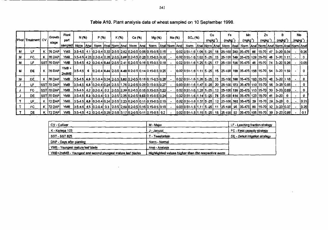
141

Table A10. Plant analysis data of wheat sampled on 10 September 1998.

Pivot

M

M

M

M

M

J

J

J

T

T

T

Treatment

LF

FC

LF

DE

DE

LF

FC

DE

LF

FC

DE

CV

K

K

SST

K

K

SST

SST

SST

K

K

K

Growth

stage

76 DAP

76 DAP

76 DAP

76 DAP

76 DAP

70 DAP

70 DAP

70 DAP

72 DAP

72 DAP

72 DAP

Plant

part

sampled

YMB

YMB

YMB

YMB +

2ndMB

YMB

YMB

YMB

YMB

YMB

YMB

YMB

N(%)

Norm

3.5-4.5

3.5-4.5

3.5-4.5

3.5-4.5

3.5-4.5

3.5-4.5

3.5-4.5

3.5-4.5

3.5-4.5

3.5-4.5

3.5-4.5

Anal

4.1

4.25

4.2

6

4.9

4.6

4 ?

5.2

4.6

4.5

4.2

P(%)

Norm

0.2-0.4

0.2-0.4

0.2-0.4

0.2-0.4

0.2-0.4

0.2-0.4

0.2-0.4

0.2-0.4

0.2-0.4

0.2-0.4

0.2-0.4

Anal

0.32

0.26

0.44

0.44

0.24

0.24

0?

0.3

0.34

0 3

0.29

K(%)

Norm

2-3.5

2-3.5

2-3.5

2-3.5

2-3.5

2-3.5

2-3.5

2-3.5

2-3.5

2-3.5

2-3.5

Anal

2.82

3.66

7 41

4.43

3.82

1.76

5 30

2.25

2.23

?R9

3.17

Ca(%)

Norm

0.2-0.5

0.2-O.5

0.2-0.5

0.2-0.5

0.2-0.5

0.2-0.5

0.2-0.5

0.2-0.5

0.2-0.5

0.2-0.5

0.2-0.5

Anal

0.08

0.28

nifi

014

0.18

0.28

0 18

0.63

0.11

nifi

0.11

Mg(%)

Norm

0,15-0.5

0.15-0.5

0,15-0.5

0.15-0.5

0,15-0.5

0,15-0.5

0.15-0.5

0.15-0.5

0.15-0.5

0.15-0.5

0.15-0.5

Anal

0.15

0.18

018

0.25

0.26

0.27

0.22

0.24

0.15

ma0.2

Na(%)

Norm

_

-

_

-

Anal

0.02

0.02

nn?

0.02

0.02

0.03

0.02

0.02

0.02

0.03

0.02

SO4 (%)

Norm

0,51-1.6

0.51-1.6

0.51-1.6

0.51-1.6

0.51-1.6

0.51-1.6

0.51-1.6

0.51-1.6

O.5M.6

0.51-1.6

0.51-1.6

Anal

1,06

1.02

1.7S

1.11

1.26

1.47

1.28

1.14

1.37

1.11

1.15

Cu

(makg1)

Norm

5-25

5-25

5-25

5-25

5-25

5-25

5-25

5-25

5-25

5-25

5-25

Anal

13

15

17

15

15

20

12

75

12

11

18

Fe

(mgkg"1)

Norm

25-100

25-100

25-100

25-100

25-100

25-100

25-100

25-100

25-100

25-100

25-100

Anal

203

149

126

159

158

173

135

414

102

95

92

Mn

(mgkg-1)

Norm

35-475

35-475

35-475

35-475

35-475

35-475

35-475

35-475

35-475

35-475

35-475

Anal

66

129

48

156

183

110

113

123

29

80

105

Zn

(mgkg1)

Norm

15-70

15-70

15-70

15-70

15-70

15-70

15-70

15-70

15-70

15-70

15-70

Anal

47

48

74

54

48

56

30

41

29

32

39

B

(mgkg-1)

Norm

3-20

3-20

3-20

3-20

3-20

3-20

3-20

3-20

3-20

3-20

3-20

Anal

0.34

1.11

0.26

1.59

1.18

0.65

0.69

0

0

0.37

0.99

Mo

(mgkg1)

Norm

_

_

-

Anal

0.26

0

0.05

0

0

0

0

0

0.21

0.25

0.1

CV - Cultivar

K-Kariega103

SST - SST 825

DAP - Days after planting

YMB - Youngest mature leaf blade

YMB+2ndMB - Youngest and second youngest mature leaf blades

M - Major

J - Jacuzzi

T - Tweefontein

Norm - Normal

Anal - Analysis

Highlighted values higher than the respective norm

LF - Leaching fraction strategy

FC - Field capacity strategy

DE - Deficit irrifjation strategy

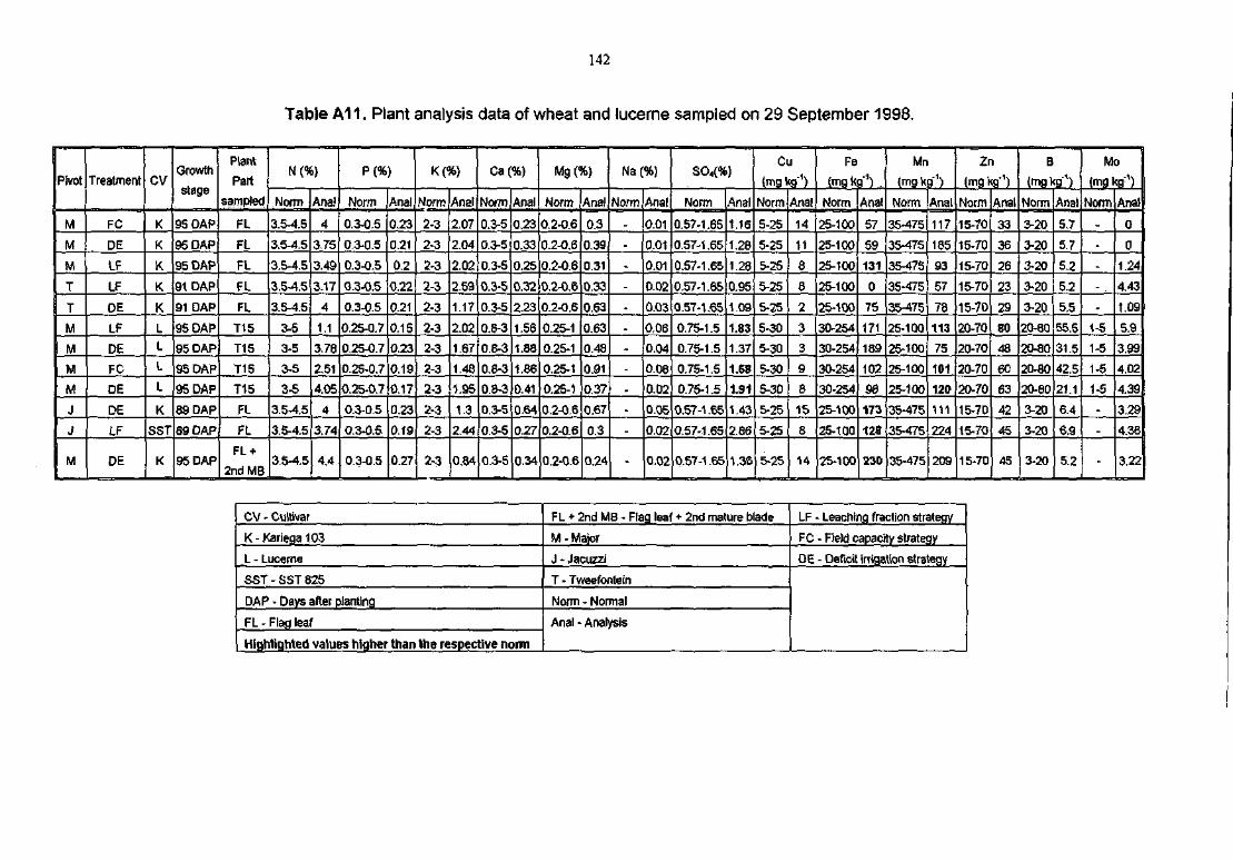
142

Table A11. Plant analysis data of wheat and lucerne sampled on 29 September 1998.

Pivot

M

M

M

T

T

M

M

M

M

J

J

M

Treatment

FC

DE

LF

LF

DE

LF

DE

FC

DE

DE

LF

DE

CV

K

K

K

K

K

L

L

L

L

K

SST

K

Growth

stage

95 DAP

95 DAP

95 DAP

91 DAP

91 DAP

95 DAP

95 DAP

95 DAP

95 DAP

89 DAP

89 DAP

95 DAP

Plant

Part

sampled

FL

FL

FL

FL

FL

T15

T15

T15

T15

FL

FL

FL +

2nd MB

N(%)

Norm

3.5-4.5

3.5-4.5

3.5-4.5

3.5-4.5

3.5-4.5

3-5

3-5

3-5

3-5

3.5-4.5

3.5-4.5

3.5-4.5

Ana!

4

3.75

3.49

3.17

4

1.1

3.76

2.51

4,05

4

3.74

4,4

PC%>

Norm

0.3-0.5

0.3-0.5

0.3-0.5

0.3-0.5

0.3-0.5

0.25-0.7

0.25-0.7

0.25-0.7

0.25-0.7

0.3-0.5

0.3-0.5

0.3-Q.5

Anal

0.23

0.21

0.2

0.22

0.21

0.15

0.23

0.19

0.17

0.23

0.19

0.27

K(%)

Norm

2-3

2-3

2-3

2-3

2-3

2-3

2-3

2-3

2-3

2-3

2-3

2-3

Anal

2.07

2.04

2.02

2.59

1.17

2.02

1.67

1.48

1.95

1.3

2.44

0.84

Ca(%)

Norm

0.3-5

0.3-5

0.3-5

0.3-5

0.3-5

0.8-3

0.8-3

0.8-3

0.8-3

0.3-5

0.3-5

0.3-5

Anal

0.23

0.33

0.25

0.32

2.23

1.56

1.88

1.86

0.41

0.64

0.27

0.34

Mg(%)

Norm

0.2-0.6

0.2-0.6

0.2-0.6

0.2-0.6

0.2-0.6

0.25-1

0.25-1

0.25-1

0.25-1

0.2-0.6

0.2-0.6

0.2-0.6

Anal

0.3

0.39

0.31

0.33

0.63

0.63

0.48

0.91

0.37

0.67

0.3

0.24

Na(%)

Norm_

_

_

-

Anal

0.01

0.01

0.01

0.02

0.03

0.06

0.04

0.08

0.02

0.05

0.02

0.02

Norm

0.57-1.65

0.57-1.65

0.57-1.65

0.57-1.65

0.57-1.65

0.75-1.5

0.75-1.5

0.75-1.5

0.75-1.5

0.57-1.65

0.57-1.65

0,57-1.65

Anal

1,16

1.28

1.28

0.95

1.09

1.83

1.37

1.68

1.91

1.43

2.86

1.36

Cu

(mg kg"1)

Norm

5-25

5-25

5-25

5-25

U5:25_

5-30

5-30

5-30

5-30

5-25

5-25

5-25

Anal

14

11

8

8

2

3

3

9

8

15

8

14

Fe

(rngkg'1)

Norm

25-100

25-100

25-100

25-100

25-100

30-254

30-254

30-254

30-254

25-100

25-100

25-100

Anal

57

59

131

0

75

171

189

102

98

173

128

230

Mn

(mg kg"1)

Norm

35-475

35-475

35-475

35-475

35-475

25-100

25-100

25-100

25-100

35-475

35-475

35-475

Anal

117

185

93

57

7S

113

75

101

120

111

224

209

Zn

(mgkg'1)

Norm

15-70

15-70

15-70

15-70

15-70

20-70

20-70

20-70

20-70

15-70

15-70

15-70

Anal

33

36

26

23

29

80

48

60

63

42

45

45

B

(mgkg1)

Norm

3-20

3-20

3-20

3-20

3-20

20-80

20-80

20-80

20-60

3-20

3-20

3-20

Anal

5.7

5.7

5.2

5.2

5.5

55.5

31.5

42.5

21.1

6.4

6.9

5.2

Mo

Norm

_

_

_

1-5

1-5

1-5

1-5

_

-

Anal

0

0

1.24

4.43

1.09

5.9

3.99

4.02

4.39

3.29

4.3B

3.22

CV - Cultivar

K-Kariega103

L - Lucerne

SST - SST 825

DAP - Days after planting

FL - Flag leaf

Highlighted values higher than the respective norm

FL + 2nd MB - Flag leaf + 2nd mature blade

M - Major

J - Jacuzzi

T - Tweefontein

Norm - Normal

Anal - Analysis

LF - Leaching fraction strategy

FC - Field capacity strategy

DE - Deficit irrigation strategy

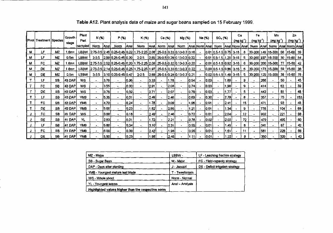
143

Table A12. Plant analysis data of maize and sugar beans sampled on 15 February 1999.

Pivot

M

M

M

M

M

T

T

T

T

T

T

J

J

J

J

J

Treatment

LF

LF

FC

DE

DE

LF

FC

DE

LF

FC

DE

FC

DE

LF

FC

DE

Species

MZ

MZ

MZ

MZ

MZ

SB

SB

SB

SB

SB

SB

SB

SB

SB

SB

SB

Growth

stage

1.6m+

0.5m

1.6m+

1.6m+

0.5m

43 DAP

43 DAP

43 DAP

43 DAP

43 DAP

43 DAP

41 DAP

41 DAP

41 DAP

41 DAP

41 DAP

Plant

Part

sampled

LBBW

LBBW

LBBW

LBBW

LBBW

WS

WS

WS

YMB

YMB

YMB

WS

YL

YMB

YMB

YMB

N(%)

Norrn

2.75-3.5

3-3.5

2.75-3.5

2.75-3,5

3-3.S

_

-

Anal

2.45

2.99

2.52

?14

3.10

3.76

3.S5

3.75

5.35

4.70

5.00

3.68

2.83

5.60

6.00

5.80

P(%)

Norm

0.25-0.45

0.25-0.45

0.25-0.45

0.25-0.45

0.25-0.45

_

_

_

-

Anal

0.22

0.30

0.20

n?s

0.47

0.3S

0.30

0.32

0.31

0.24

0.23

0.18

0.31

0.34

0.30

0.23

K(%)

Norm

1.75-2.25

2-2.5

1.75-2.25

1.75-2.25

2-2.5

_

_

_

-

Anal

2.08

2.65

2.09

197

2.89

3.33

2.91

2.71

2.49

1.78

1.82

2.49

1.72

3.10

2.43

1.98

Ca(%)

Norm

.25-0.5

.25-0.5

.25-0.5

.25-0.5

.25-0.5

_

_

_

_

-

Anal

0.33

0.29

0.32

033

0.28

1.78

2.08

2.07

2.46

3.09

2.95

2.46

2.21

2.31

1.98

2.46

Mg{%)

Norm

0.13-0.3

0.13-0.3

0.13-0.3

0.13-0.3

0.13-0.3

_

_

_

_

_

_

_

_

-

Anal

0.16

0.22

0.20

n??

0.21

0.54

0.74

0.79

0.69

1.06

1.21

0.72

0.76

0.55

0.96

1.11

Na(%)

Norm

_

_

_

_

„

_

_

-

Anal

0.01

0.01

0.01

O.OO

0.02

0.03

0.03

0.03

0.30

0.01

0.01

0.01

0.02

0.01

0.01

0.01

S O , (%)

Norm

0.5-1.5

0.5-1.5

0.5-1.5

0.5-1.5

0.5-1.5

_

_

_

_

_

_

_

_

-

Anal

0.75

1.20

0.92

0.86

1.49

1.89

1.98

1.77

2.79

2.41

1.34

2.04

2.03

1.49

1.61

1.22

CU

(mgkg1)

Norm

3-15

3-15

3-15

3-15

3-15

_

_

-

Anal

8

5

6

6

5

9

9

6

8

15

9

12

72

8

11

9

Fe

(fng kg"1)

Norm

30-200

30-200

30-200

30-200

30-200

_

_

_

_

-

Anal

149

227

200

173

125

266

414

443

357

471

776

902

479

341

581

350

Mn

(mg kg"1)

Norm

15-300

15-300

15-300

15-300

15-300

-

_

-

Anal

56

30

77

59

38

50

63

81

75

93

104

221

495

87

228

320

Zn

(mg Kg"1)

Norm

15-60

15-60

15-60

15-60

15-60

_

-

Ana!

39

54

42

38

78

45

39

48

153

48

89

98

60

42

56

42

MZ - Maize

SB - Sugar Bean

DAP - Days after planting

YMB - Youngest mature leaf blade

WS - Whole shoot

YL - Youngest leaves

Highlighted values higher than the respective norm

LBBW-

M - Major

J - Jacuzzi

T - Tweefontein

Norm - Normal

Anal - Analysis

LF - Leaching fraction strategy

FC - Field capacity strategy

DE - Deficit irrigation strategy

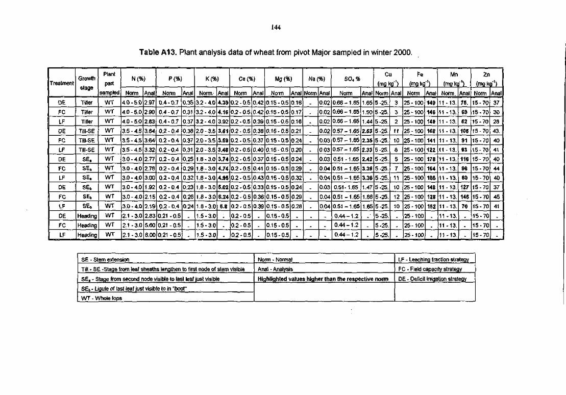
144

Table A13. Plant analysis data of wheat from pivot Major sampled in winter 2000.

Treatment

DE

FC

LF

DE

FC

LF

DE

FC

LF

DE

FC

LF

DE

FC

LF

Growth

stage

I TiHer

Tiller

Tiller

Till-SE

Till-SE

Till-SE

SE.

SEa

SE,

SEb

SEb

SE6

Heading

Heading

Heading

Plant

part

sampled

WTWT

WT

WT

WT

WT

WT

WT

WT

WT

WT

WT

WT

WT

WT

N{%)

Norm

4.0-5.0

4.0 - 5.0

4,0 - 5.0

3.5 - 4.5

3.5 - 4.5

3.5 - 4.5

3.0 - 4.0

3.0 - 4.0

3.0 - 4.0

3.0 - 4.0

3.0 - 4.0

3.0 - 4.0

2.1 - 3.0

2.1 -3.0

2.1-3.0

Anal

2.97

2.90

2.83

3.64

3.64

3.32

2.77

2.78

3.00

1.92

2.15

2.19

2.83

5.60

6.00

P (%)

:Norm

0.4 - 0.7

0.4-0.7

0.4-0.7

0.2 - 0.4

0.2-0.4

0.2 - 0.4

0.2 - 0.4

0.2 - 0.4

0.2 - 0.4

0.2-0.4

0.2 - 0.4

0.2 - 0,4

0.21 -0.5

0.21 - 0.5

0.21 - 0.5

Anal

0.35

0.31

0.37

0.38

0.37

0.31

0.25

0.29

0.32

0.23

0.26

0.24

_

_

-

K(%)

Norm:

3.2 - 4.0

3.2 - 4.0

3.2 - 4,0

2.0 - 3.5

2.0-3.5

2.0 - 3.5

1.8-3.0

1.8 - 3.0

1.6 - 3.Q

1.8 - 3.0

1.8 - 3.0

1.8-3.0

1,5 - 3.0

1.5-3.0

1.5-3.0

Anal

4.39

4.16

3.92

3.61

3.59

3.48

3.74

4.74

4.9S

5.02

6.24

5.8_

_

-

Ca(%)

Norm

0.2-0.5

0,2 - 0.5

0.2 - 0.5

0.2-0.5

0.2 - 0.5

0.2 - 0.5

0.2 - 0.5

0.2-0,5

0.2-0.5

0.2-0.5

0.2-0.5

0.2 - 0.5

0.2 - 0.5

0.2-0.5

0.2 - 0.5

Anal

0.42

0.42

0.39

0.38

0.37

0.40

0.37

0.41

0.43

0.33

0.36

0.39

_

-

Mg(%)

Norm

0.15-0.5

0.15-0.5

0.15-0.5

0.15-0.5

0.15-0.5

0,15-0.5

0.15-0.5

0.15-0.5

0.15-0.5

0.15-0.5

0.15-0.5

0.15-0.5

0.15-0.5

0.15-0.5

0.15-0.5

Anal

0.16

0.17

0.16

0.21

0.24

0.20

0.24

0.29

0.32

0.24

0.29

0.28

-

Na(%)

Norm

_

_

_

-

Anal

0.02

0.02

0.02

0.02

0.03

0.03

0.03

0.04

0.04

0.03

0.04

0.04

_

-

SO4%

Norm

0.66-1.65

0.66 -1.65

0.66 -1.65

0.57 -1.65

0.57-1.65

0.57 - 1.65

0.51 -1.65

0.51-1.65

0.51 -1.65

0.51-1.65

0.51-1.65

0.51 -1.65

0.44-1.2

0.44-1.2

0.44-1.2

Anal

1.65

1.50

1.44

2.53

2.35

2.33

2.42

3.39

3.36

1.47

1.86

1.65

-

Cu

(mg kg"1)

Norm

5-25.

5-25.

5-25.

5-25.

5-25.

5-25.

5-25,

5-25.

[5-25.

5-25.

5-25.

5-25.

5-25.

5-25.

5-25.

Anal

3

3

2

11

10

S

5

7

11

10

12

10

-

Fe

(mg kg"')

Norm

25-100

25 -100

25-100

25-100

25-100

25-100

25- 100

25-100

25-100

25-100

25-100

25-100

25-100

25-100

25-100

Anal

149

146

140

168

141

122

178

164

185

148

128

152

-

Mn

(mg Kg"')

Norm.

11-13.

11 -13.

11-13.

11-13.

11-13.

11 -13.

11-13.

11 -13.

11-13.

11-13.

11 -13.

11 -13.

11 -13.

11 -13.

11-13.

Anal

75.

63

62

106

91

93

116

96

60

127

145

70

-

Zn

{mg kg"1)

Norm

15-70

15-70

15-70

15-70

15-70

15-70

15-70

15-70

15-70

15-70

15-70

15-70

15-70

15-70

15-70

Ana!

37

30

28

43.

40

41

40

44

40

37

45

41

_

_

-

SE - Stem extension

Till - SE -Stage from leaf sheaths lengthen to first node of stem visible

SEa - Stage from second node visible to last leaf just visible

SEt - Ligule of last leaf just visible to in "boot"

WT - Whole tops

Norm - Normal

Anal - Analysis

Highlighted values higher than the respective aorm

LF - Leaching fraction strategy

FC - Field capacity strategy

OE - Deficit irrigation strategy

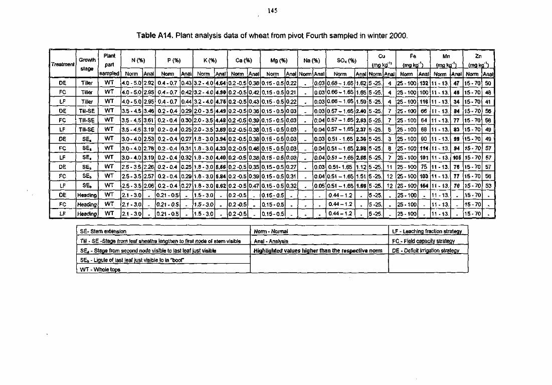
145

Table A14. Plant analysis data of wheat from pivot Fourth sampled in winter 2000.

Treatment

DE

FC

LF

DE

FC

LF

DE

FC

LF

DE

FC

LF

DE

FC

LF

Growth

stage

Tiller

Tiller

Tiller

Till-SE

TIII-SE

Till-SE

SE,

SE.

SE,

SEb

SEb

SEb

Heading

Heading

Heading

Plant

part

sampled

WT

WT

WT

WT

WT

WT

WT

WT

WT

WT

WT

WT

WT

WT

WT

N(%)

Norm

4.0 - 5.0

4.0 - 5.0

4.0 - 5.0

3.5-4.5

3.5 - 4.5

3.5 - 4.5

3.0 - 4.0

3.0-4.0

3.0 - 4.0

2.5-3.5

2.5-3.5

2.5-3.5

2.1 -3.0

2.1 - 3.0

2.1 - 3.0

Anal

2.92

?flS

2.95

3.46

3.61

3.19

2.53

2.78

3.19

2.26

2.57

2.06

_

-

P(%)

Norm

0.4-0.7

0.4-0.7

0.4-0.7

0.2 - 0.4

0.2 - 0.4

0.2-0.4

0.2-0.4

0.2 - 0.4

0.2-0.4

0.2 - 0.4

0.2 - 0.4

0.2 - 0.4

0.21 - 0.5

0.21-0.5

0.21-0.5

Anal

0.43

0 4?

0.44

0.29

0.30

0.25

0.27

0.31

0.32

0.25

0.29

0.27

-

K(%)

Norm

3.2 - 4.0

3.2 - 4.0

3.2-4.0

2.0-3.5

2.0 - 3.5

2.0-3.5

1.8 - 3,0

1.8 - 3.0

1.8-3.0

1.8-3.0

1.8 - 3.0

1.8-3.0

1.5-3.0

1.5-3,0

1.5-3.0

Anal

4.64

4,90

4.75

4.49

4.4S

3.69

3.94

4.33

4.40

5.56

5.84

6.62

_

-

Ca(%)

Norm

0.2 -0.5

0.2 -0.5

0.2 -0.5

0.2 -0.5

0.2 -0.5

0.2 -0.5

0.2 -0.5

0.2 -0.5

0.2 -0.5

0.2 -0.5

0.2 -O.5

0.2-0.5

0.2 -0.5

0.2 -0.5

0.2-0.5

Anal

0.38

0 4?

0.43

0.36

0.39

0,38

0.38

0.46

0.38

0.35

0 39

0.47

_

-

Mg (%)

Norm

0.15-0.5

0.15-0.5

0.15-0.5

0.15-0.5

0.15-0.5

0.15-0.5

0.15-0.5

0.15-0.5

0.1S-0.5

0.15-0.5

0.15-0.5

0.15-0.5

0.15-0.5

0.15-0.5

0.15-0.5

Anal

0.22

0?1

0.22

0.03

0.03

0.03

0.03

0.03

0.03

0.27

m i

0.32

-

Na(%)

Norm

_

_

_

_

_

_

-

Anal

0.03

0.03

0.03

0.03

0.04

0.04

0.03

0.04

0.O4

0.03

0 04

0.05

_

_

-

SO4{%)

Norm

0.66-1.65

0.66 -1.65

0.66 ~ 1.65

0.57 -1.65

0.57-1.65

0.57 -1.65

0.51 -1.65

0.51 -1.65

0.51-1.65

0.51-1.65

0.51-1.65

0.51 -1.65

0.44-1.2

0.44 -1 .2

0.44-1.2

Anal

1.62

1.65

1.59

2.40

2.63

2.37

2.36

2.98

2.65

1.12

151

1.66

„

-

Cu

(mgkg;11

Norm

5-25.

5-25.

5-25.

5-25.

5-25.

5-25.

5-25.

5-25.

5-25.

5-25.

5-25.

5-25.

5-25.

5-25.

5-25.

Anal

4

4

4

7

7

5

3

8

7

11

12

12

-

Fe

<mg kg"1)

Norm

25-100

25-100

25-100

25-100

25-100

25-100

25-100

25-10025-100

25-100

25-100

25-100

25-100

25-100

25-100

Anal

132

100

116

66

64

68

90

114101

75

103

154

.

_

-

Mn

(mg kg/1)

Norm

11-13.

11 -13.

11-13.

11-13.

11 -13.

11-13.

11 -13.

11-13.

11 -13.

11-13.

11-13.

11-13.

11-13.

11-13.

11-13.

Anal

47

45

34

84

77

33

99

94

105

75

77

76

-

Zn

{mg kg"')

Norm

15-7015-7015-7015-7015-7015-7015-7015-7015-70

15-70

15-70

15-70

15-70

15-70

15-70

Anal

50

48

41

56

58

49

49

57

57

57

56

53

-

SE- Stem extension

Till - SE -Stage from leaf sheaths lengthen to first node of stem visible

SEjt - Stage from second node visible to last leaf just visible

SEb - Ligule of last leaf just visible to in "boot"

WT - Whole tops

Norm - Normal

Anal - Analysis

Highlighted values higher than the respective norm

LF - Leaching fraction strategy

FC - Field capacity strategy

DE - Deficit irrigation strategy

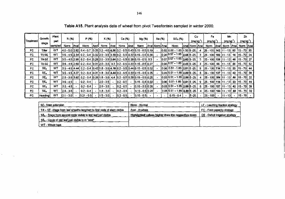
146

Table A15. Plant analysis data of wheat from pivot Tweefontein sampled in winter 2000.

Treatment

FC

FC

FC

FC

FC

FC

FC

FC

FC

FC

FC

Growth

stage

Tiller

Til-SE

Til-SE

Til-SE

SEB

SE,

SE.

SEb

SEb

SE>

Heading

Plant

part

sampled

WT

WT

WT

WT

WT

WT

WT

WT

WT

WT

WT

N(%)

Norm

4.0 - 5.0

3.5 - 4.5

3.5 - 4.5

3.5 - 4.5

3.5 - 4.5

3.5 - 4.5

2.5-3.5

3.5-4.5

3.5 - 4.5

2.5 - 3.5

2.1 - 3.0

Anal

2.92

2.34

2.99

?fiq

4.44

4.37

3.92

-

-

-

•

P{%)

Norm

0.4 - 0.7

0.2 - 0.4

0.2-0.4

0.2 - 0.4

0.2 - 0.4

0.2 - 0.4

0,2-0.4

0.2 - 0,4

0.2 - 0.4

0.2 - 0.4

0.21-0,5

Anal

0.35

0.32

0.28

(131

0.42

0.31

0.26

-

-

-

-

K{%)

Norm

3.2 - 4.0

2.0 - 3.5

2,0 - 3,5

2.0 - 3.5

1.8-3,0

1.6 - 3.0

1.8-3,0

2.0 - 3.5

2.0 - 3.5

1.8 - 3,0

1,5 - 3.0

Anal

4.36

3.39

3.64

33

4.19

4.44

4.4

-

-

-

-

Ca{%)

Norm

0.2 - 0.5

0.2-0.5

0.2-0.5

0.2 - 0.5

0.2 - 0.5

0.2 - 0,5

0.2-0.5

0.2-0.5

0.2 - 0,5

0.2-0.5

0.2-0,5

Anal

0.43

0.32

0.29

0 33

0.44

0.33

0,39

-

-

-

-

Mg(%)

Norm

0.15-0.5

0.15-0.5

0.15-0.5

0.15-0.5

0.15-0.5

0.15-0.5

0.15-0.5

0.15-0.5

0.15-0.5

0.15-0.5

0,15-0.5

Anal

0.19

0.30

0.3

n?7

0.32

0.35

0.25

0.32

0.35

0.25

-

Na(%)

Norm

-

-

-

-

-

-

-

-

-

-

Anal

0.02

0.20

0.07

0.06

0.06

0.05

0.05

0.06

0.05

0.05

-

SO4 (%)

Norm

0.66-1.650.57-1.65

0.57-1.65

0.57 -1.65

0.51 -1.65

0.51 - 1.65

0.51 -1.65

0.51-1.65

0.51-1.65

0.51 -1.65

0.15-0.4

Anal

1.50

2.65

2.63

2.43

2.81

2.89

2.89

2.81

2.89

2.89

-

Cu

(mp kg"1)

Norm

5-25.

5-25.

5-25.

5-25.

5-25.

5-25,

5-25.

5-25.

5-25.

5-25.

5-25.

Anal

4

3

3

3

9

8

4

9

6

4

-

Fe

(mg kg"1)

Norm

25-100

25-100

25-100

25-100

25-100

25-100

25-100

,25-100

25-100

25-100

25-100

Anal

142

102

125

86

114

137

154

114

137

154

-

Mn

(mgkg"1)

Norm

11 -13

11-13

11-13

11-13

11 - 13

11 -13

11 -13

11 -13

11-13

11-13

11 -13

Anal

52

14

48

20

23

42

40

23

42

40

•

Zn

_lmgk

Norm

15-70

15-70

15-70

15-70

15-70

15-70

15-70

15-70

15-70

15-70

15-70

<J"')Anal

35

24

27

32

44

39

32

44

39

32

-

SE- Stem extension

Tiil - SE -Stage from leaf sheaths lengthen to first node of stem visible

SE, - Stage from second node visible to last leaf just visible

SEs - Ugule of last leaf just visible to in "boor

WT - Whole tops

Norm - Normal

Anal - Analysis

Highlighted values higher than the respecttve norm

LF - Leaching fraction strategy

FC - Field capacity strategy

DE - Deficit irrigation strategy

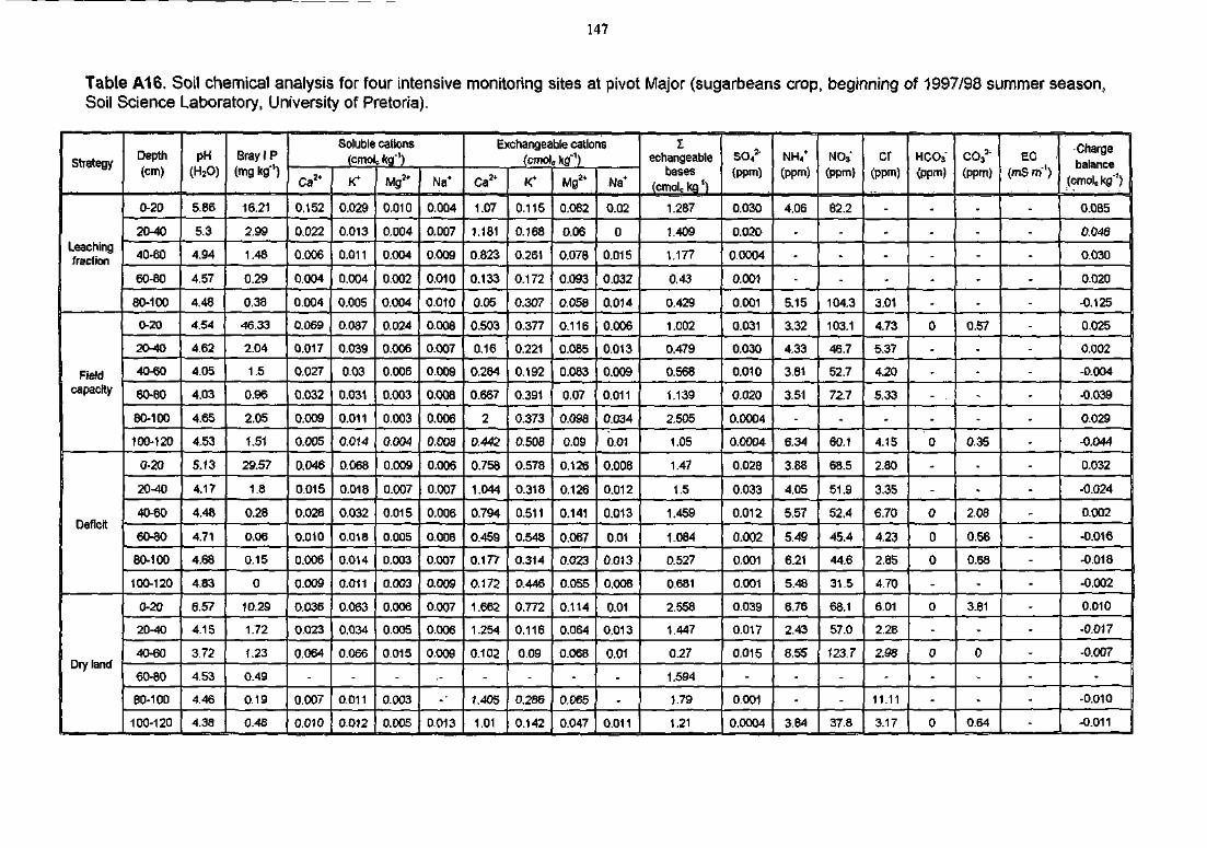
147

Table A16. Soil chemical analysis for four intensive monitoring sites at pivot Major (sugarbeans crop, beginning of 1997/98 summer season,Soil Science Laboratory, University of Pretoria).

Strategy

Leachingfraction

Fieldcapacity

Deficit

Dry (and

Depth(cm)

0-20

20-40

40-60

60-80

80-100

0-20

20-40

40-60

60-60

80-100

100-120

0-20

20-40

40-60

60-80

80-100

100-120

0-20

20-40

40-60

60-80

80-100

100-120

pH(H2O)

5.86

5.3

4.94

4.57

4.48

4.54

4.62

4.05

4.03

4.65

4.53

5.13

4.17

4.48

4.71

4.68

4.83

6.57

4.15

3.72

4.53

4.46

4.38

Bray IP(mg kg1)

16.21

2.99

1.48

0.29

0.38

46.33

2.04

1.5

0.96

2.05

1.51

29.57

1.8

0.28

0.06

0.15

0

10.29

1.72

1.23

0.49

0.19

0.46

Soluble cations(cmolckg1)

0.152

0.022

0.006

0.004

0.004

0.069

0.017

0.027

0.032

0.009

0.005

0.046

0.015

0.028

0.010

0.006

0.009

0.036

0.023

0.064

-

0.007

0.010

K4

0.029

0.013

0.011

0.004

0.005

0.087

0.039

0.03

0.031

0.011

0.014

0.068

0.018

0.032

0.018

0.014

0.011

0.063

0.034

0.066

-

0.011

0.012

Mg2*

0.010

0.004

0.004

0.002

0.004

0.024

0.006

0.006

0.003

0.003

0.004

0.009

0.007

0.015

0.005

0.003

0.003

o.ooe0.005

0.015

-

0.003

0.005

Na*

0.004

0.007

0.009

0.010

0.010

0.008

0.007

0.009

0.008

0.006

0.008

0.006

0.007

0.006

0.008

0.007

0.009

0.007

0.006

0.009

.-

-'

0.013

Exchangeable cations(cmole kg"1)

Ca2t

1.07

1.181

0.823

0.133

0.05

0.503

0.16

0.284

0.667

2

0.442

0.758

1.044

0.794

0.459

0.177

0.172

1.662

1.254

0.102

-

1.405

1.01

K*

0.115

0.168

0.261

0.172

0.307

0.377

0.221

0.192

0.391

0.373

0.508

0.578

0.318

0.511

0.548

0.314

0.446

0.772

0.116

0.09

-

0,286

0.142

Mg2*

0.082

0.06

0.078

0.093

0.058

0.116

0.085

0.083

0.07

0.096

0.09

0.126

0.126

0.141

0.067

0.023

0.055

0.114

0.064

0.068

-

0.065

0.047

Na*

0.02

0

0.015

0.032

0.014

0.006

0.013

0.009

0.011

0.034

0.01

0.008

0.012

0.013

0,01

0.013

0.008

0.01

0.013

0.01

-

-

0.011

Iechangeable

bases(cmolc kg *)

1.287

1.409

1.177

0.43

0.429

1.002

0.479

0.568

1.139

2.505

1.05

1.47

1.5

1.459

1.084

0.527

0.681

2.558

1.447

0.27

1.594

1.79

1.21

SO4*{ppm)

0.030

0.020

0.0004

0.001

0.001

0.031

0.030

0.010

0.020

0.0004

0.0004

0.028

0.033

0.012

0.002

0.001

0.001

0.039

0.017

0.015

-

0.001

0.0004

NH4*(ppm)

4.06

-

-

-

5.15

3.32

4.33

3,81

3.51

-

6.34

3.88

4.05

5.57

5.49

6.21

5.48

6.76

2.43

8.55

-

-

3.84

NO3'(ppm)

82.2

-

-

-

104.3

103.1

46.7

52.7

72.7

-

60.1

68.5

51.9

52.4

45.4

44.6

31.5

68.1

57.0

123.7

-

-

37.8

cr(ppm)

-

-

-

-

3.01

4.73

5.37

4.20

5.33

-

4.15

2.80

3.35

6.70

4.23

2.85

4.70

6.01

2.28

2.96

-

11.11

3.17

HCO3"(ppm)

-

-

-

-

-

0

-

-

- ,

-

0

-

-

0

0

0

-

0

-

0

-

-

0

co 33 i

(ppm)

-

-

-

-

-

0.57

-

-

-

0.35

-

-

2.08

0.56

0.68

-

3.81

-

0

-

-

0.64

EC(ms m"1)

-

-

-

-----

--

-

-

-

-

----

---

-

-

Chargebalance

(cmolekg'')

0.085

0.046

0.030

0.020

-0.125

0.025

0.002

-0.004

-0.039

0.029

-0.044

0.032

-0.024

0.002

-0.016

-0.018

-0.002

0.010

-0.017

-0.007

-

-0.010

-0.011

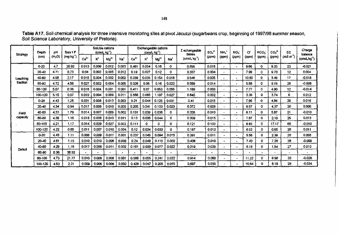
148

Table A17. Soil chemical analysis for three intensive monitoring sites at pivot Jacuzzi (sugarbeans crop, beginning of 1997/98 summer season,Soil Science Laboratory, University of Pretoria).

Strategy

Leachingfraction

Fieldcapacity

Deficit

Depth(cm)

0-20

20-40

40-60

60-80

80-100

100-120

0-20

20-40

40-60

60-80

80-100

100-120

0-20

20-40

40-60

60-80

80-100

100-120

pH(H2PJ

4.7

4.71

4.56

4.72

5.07

5.15

4.43

4.34

4.33

4.38

4.21

4.22

4.43

4,61

4.29

5.38

4.73

4.53

Bray I P

(mg kg'1)

20.92

0.73

2.17

4.58

036

0.07

1.25

0.94

1.79

1.16

1.17

0.65

1.11

1.15

1.16

38.92

21.77

2.21

Soluble cations(cmolc kg'1)

Ca*

0.013

0.04

0.016

0.027

0.018

0.010

0.031

0.017

0.014

0.013

0.014

0.011

0.008

0.010

0.017

-

0.010

0.009

0.009

0.002

0.004

0.002

0.004

0.004

0.008

0.006

0.007

0.008

0.029

0.007

0.009

0.010

0.008

-

0.008

0.006

MgI+

0.012

0.005

0.002

0.004

0.001

0.009

0.013

0.010

0.009

0.010

0.027

0.010

0.011

0.008

0.011

-

0.008

0.006

Na*

0.003

0.012

0.002

0.005

0.001

0.011

0.003

0.006

0.002

0.011

0.002

0.004

0.001

0.009

0.002

-

0.001

0.002

Exchangeable cations(cmolc kg"1)

Ca"

0.461

0.19

0.339

0.326

0.411

0.556

0.21

0.205

0.131

0.13

0.111

0.12

0.237

0.24

0.181

-

0.586

0.429

0.054

0.027

0.035

0.05

0.07

0.065

0.044

0.041

0.039

0.035

0

0.034

0.045

0.049

0.039

-

0.055

0.047

Mg*

0.18

0.12

0.154

0.16

0.653

J.197

0.125

0.103

0.036

0.044

0

0.033

0.094

0.115

0.077

-

0.241

0.206

Na*

0

0

0.018

0.023

0.055

0.027

0.031

0.023

0

0

0

0

0.015

0.002

0.022

-

0.022

0.015

I echangeablebases

(cmolckg1)

0.695

0.337

0.546

0.559

1.189

0.845

0.41

0.372

0.206

0.209

0.121

0.187

0.391

0.406

0.319

-

0.914

0.697

SO,2"(ppm)

.0.018

0.004

0.005

0.014

0.003

0.002

0.015

0.008

0.010

0.015

0.100

0.013

0.011

0.010

0.020

-

0.060

0.030

NH4*(PPfn)

-

-

-

-

-

-

-

-

-

-

-

- •

-

-

-

-

-

-

NO3"(ppm)

-

-

-

-

-

-

-

-

-

-

-

-

-

-

-

-

-

cr(ppm)

9.66

7.99

10.60

5.58

111

3.39

7.96

6.57

8.11

7.67

8.83

6.53

5.58

7.43

8.18

-

11.22

10.64

HCO,-(ppm)

0

0

0

0

0

0

0

0

0

0

0

0

0

0

0

-

0

0

CO*2"(PPm)

9.33

9.70

3.49

9.15

4.90

3.74

4.86

4.37

5.87

2.10

17.17

0.65

2.39

7.20

1.54

-

6.98

8.19

EC(tnS tn'1)

23

12

17

26

12

6

29

20

21

25

66

26

20

36

27

-

33

29

Chargebalance

(cmoUg1)

-0.021

0.004

-0.018

-0.008

-0.014

0.012

0.016

0.006

-0.010

0.013

-0.010

0.011

0.005

-0.008

0.010

-

-0.028

-0.034

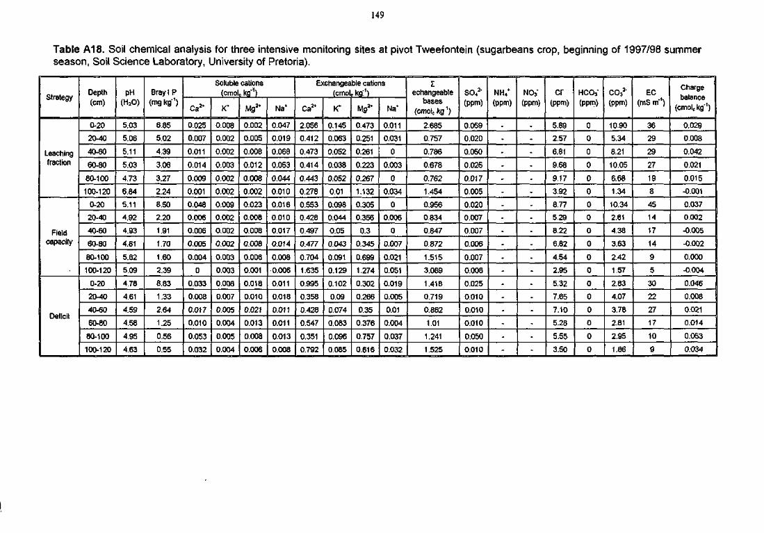
149

Table A18. Soil chemical analysis for three intensive monitoring sites at pivot Tweefontein (sugarbeans crop, beginning of 1997/98 summerseason, Soil Science Laboratory, University of Pretoria).

Strategy

Leachingfraction

Fieldcapacity

Deficit

Depth(cm)

O-20

20-40

40-60

60-80

80-100

100-120

0-20

20-40

40-60

60-80

80-100

100-120

0-20

20-40

40-60

60-80

80-100

100-120

PH<H2O)

5.03

5.06

5.11

5.03

4.73

6.84

5.11

4.92

4.93

4.81

5.62

5.09

4.78

4.61

4.59

4.58

4.95

4.63

Bray 1 P<mg kg1)

6.85

5.02

4.39

3.06

3.27

2.24

8.50

2.20

1.91

1.70

1.60

2.39

8.83

1.33

2.64

1.25

0.56

0.55

Soluble cations(cmolc kg"1)

Ca2*

0.025

0.007

0.011

0.014

0.009

0.001

0.048

0.006

0.006

0.005

0.004

0

0.033

0.008

0.017

0.010

0.053

0.032

K

0.008

0.002

0.002

0.003

0.002

0.002

0.009

0.002

0.002

0.002

0.003

0.003

0,008

0.007

0.005

0.004

0.005

0.004

Mg2*

0.002

0.005

0.008

0.012

0.008

0.002

0.023

0.008

0.008

0.008

0.006

0.001

0.018

0.010

0.021

0.013

0.008

0.006

Na*

0.047

0.019

0.068

0.053

0.044

0.010

0.016

0.010

0.017

O.OU

0.008

0.006

0.011

0.018

0.011

0.011

0.013

0.008

Exchangeable cations(cmolc kg:1)

Ca24

2.056

0.412

0.473

0.414

0.443

0.278

0.553

0.428

0.497

0.477

0.704

1.635

0.995

0.358

0.428

0.547

0.351

0.792

0.145

0.063

0.052

0.038

0.052

0.01

0.098

0.044

0.05

0.043

0.091

0.129

0.102

0.09

0.074

0.083

0.096

0.085

Mg2*

0.473

0.251

0.261

0.223

0.267

1.132

0.305

0.356

0.3

0.345

0.699

1.274

0.302

0.266

0.35

0.376

0.757

0.616

Na*

0.011

0.031

0

0.003

0

0.034

0

0.006

0

0.007

0.021

0.051

0.019

0.005

0.01

0.004

0.037

0.032

Iechangeable

bases(cmole kg1)

2,685

0,757

0.786

0,678

0.762

1.454

0.956

0,834

0,847

0.872

1.515

3.089

1.418

0.719

0.862

1.01

1.241

1.525

SO,2"(ppm)

0.059

0.020

0.050

0.025

0.017

0.005

0.020

0.007

0,007

0.006

0.007

0.008

0.025

0.010

0.010 J

0.010

0.050

0.010

NH«+

(ppm)

-

-

-

-

-

-

-

-

-

-

-

-

-

-

-

NOj"(ppm)

•

-

-

-

-

-

-

-

-

-

-

-

-

-

-

-

-

-

cr(ppm)

5.89

2.57

6.81

9.68

9.17

3.92

8.77

5.29

8.22

6.82

4.54

2.95

5.32

7.65

7.10

5.28

5.55

3.50

HCO3"(ppm)

0

0

0

0

0

0

0

0

0

0

0

0

0

0

0

0

0

0

CO32"

(ppm)

10.90

5.34

8.21

10.05

6.68

1.34

10.34

2.81

4.38

3.63

2.42

1.57

2.83

4.07

3.78

2.81

2.95

1.86

EC(mS m"1)

36

29

29

27

19

8

45

14

17

14

9

5

30

22

27

17

10

9

Chargebalance

(cmolckg'1)

0.029

0.008

0.042

0.021

0.015

-0.001

0.037

0.002

-0.005

-0.002

0.000

-0.004

0.046

0.008

0.021

0.014

0.053

0.034

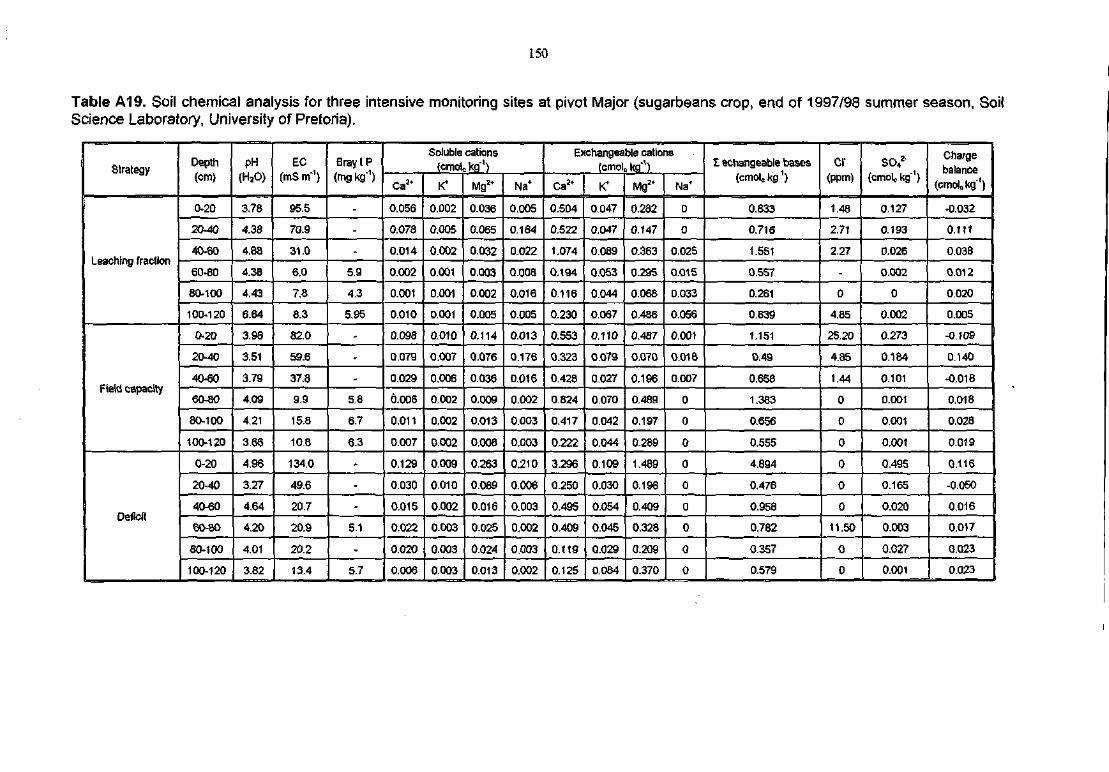
150

Table A19. Soil chemical analysis for three intensive monitoring sites at pivot Major (sugarbeans crop, end of 1997/98 summer season, SoilScience Laboratory, University of Pretoria).

Strategy

Leaching fraction

Field capacity

Deficit

Depth(cm)

0-20

20-40

40-60

60-80

80-100

100-120

0-20

20-40

40-60

60-80

80-100

100-120

0-20

20-40

40-60

60-80

80-100

100-120

pH(H2O)

3.78

4.38

4.88

4.38

4.43

6.64

3.96

3.51

3.79

4.09

4.21

3.65

4.96

3.27

4.64

4.20

4.01

3.82

EC(tnS m"1)

95.5

70.9

31.0

6.0

7.8

8.3

82.0

59.6

37.8

9.9

15.8

10B

134.0

49.6

20.7

20.9

20.2

13.4

Bray IP(mg kg"1)

-

-

-

5.9

4.3

5.95

-

-

-

5,8

6.7

6.3

-

-

-

51

-

5.7

Soluble cationsfcmolc kg')

Ca2*

0.056

0.078

0.014

0.002

0.001

0.010

0.098

0.079

0.029

6.006

0.011

O.007

0.129

0.030

0.015

0.022

0.020

0.006

(C

0,002

0.005

0.002

0.001

0.001

0.001

0.010

0.007

0.006

0.002

0.002

0.002

0.009

0.010

0.002

0.003

0.003

0.003

Mg2*

0.036

0.065

0.032

0.003

0.002

0.005

0.114

0.076

0.036

0.009

0.013

0.008

0.263

0.069

0.016

0.025

0.024

0.013

Na*

0.005

0.164

0.022

0.008

0.016

0.005

0.013

0.176

0.016

0.002

0.003

0.003

0.210

0.006

0.003

0.002

0.003

0.002

Exchangeable cations(cmolc kg-v)

Ca3t

0.504

0.522

1.074

0.194

0.116

0.230

0.553

0.323

0.428

0.824

0.417

0.222

3.296

0.250

0.495

0.409

0.119

0.125

K*

0.047

0.047

0.089

0.053

0.044

0.067

0.110

0.079

0.027

0.070

0.042

0.044

0.109

0.030

0.054

0.045

Q.029

0.084

Mg2*

0.282

0.147

0.363

0.295

0.068

0.486

0.487

0.070

0.196

0.489

0.197

0.289

1.489

0.196

0.409

0.328

0.209

0.370

Na*

0

0

0.025

0.015

0.033

0.056

0.001

0.016

0.007

0

0

0

0

0

0

0

0

0

I echangeable bases(cmolc kg1)

0.833

0.716

1.551

0.557

0.261

0.839

1.151

0.49

0.658

1.383

0.656

0.555

4,894

0.476

0.958

0.782

0.357

0.579

cr(ppm)

1.48

2.71

2.27

-

0

4.85

25.20

4.85

1.44

0

0

0

0

0

0

11.50

0

0

so/{cmolc kg1)

0.127

0.193

0.026

0.002

0

0.002

0.273

0.184

0.101

0.001

0.001

0.001

0.495

0.165

0.020

0.003

0.027

0.001

Chargebalance

(cmolokg*)

-0.032

0.111

0.038

0.012

0.020

0.005

-0.109

0.140

-0.018

0.018

0.028

0.019

0.116

-0.050

0.016

0.017

0.023

0.023

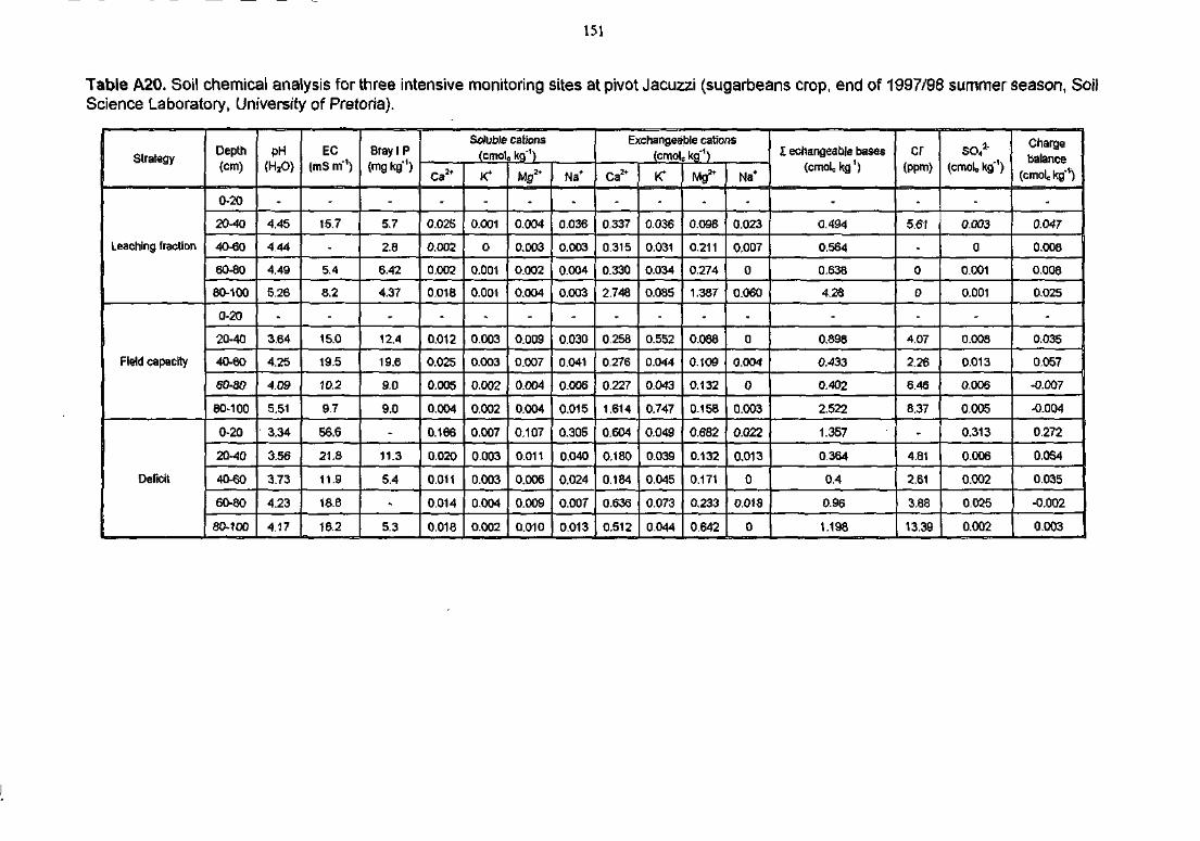
151

Table A20. Soil chemical analysis for three intensive monitoring sites at pivot Jacuzzi (sugarbeans crop, end of 1997/98 summer season, SoilScience Laboratory, University of Pretoria).

Strategy

Leaching fraction

Field capacity

Deficit

Depth(cm)

0-20

20-40

40-60

60-80

80-100

0-20

20-40

40-60

60-80

80-100

0-20

20-40

40-60

60-80

80-100

PH(HaO)

-

4.45

4.44

4.49

5.26

-

3.64

4.25

4.09

5,51

3.34

3.56

3.73

4.23

4.17

EC(mS m"')

-

15.7

-

5.4

8.2

-

15.0

19.5

10.2

9.7

56.6

21.8

11.9

18.8

16.2

Bray I P(mgkgf)

-

5.7

2.8

6.42

4.37

-

12.4

19.6

9.0

9.0

-

11.3

S.4

-

5.3

Soluble cations(cmolo kg"1)

Ca !*

-

0.025

0.002

0.002

0.018

-

0.012

0.025

O.OOS

0.004

0.166

0.020

0.011

0.014

0.018

-

0.001

0

0.001

0.001

-

0.003

0.003

0.002

0.002

0.007

0.003

0.003

0.004

0.002

Mg2t

-

0.004

0.003

0.002

0.004

-

0.009

0.007

0.004

0.004

0.107

0.011

0.006

0.009

0.010

-

0.036

0.003

0.004

0.003

-

0.030

0.041

0.006

0.015

0.305

0.040

0.024

0.007

0.013

Exchangeable cations(ctnoU kg"1)

Ca2t

-

0.337

0.315

0.330

2.748

-

0.258

0.276

0.227

1.614

0.604

0.180

0.184

0.635

0.512

K * 1

-

0.036

0.031

0.034

0.085

-

0.552

0.044

0.043

0.747

0.049

0.039

0.045

0.073

0.044

-

0.098

0.211

0.274

1.387

-

0.088

0.109

0.132

0.158

0.682

0.132

0,171

0,233

0.642

Na*

-

0.023

0.007

0

0.060

-

0

0.004

0

0.003

0.022

0.013

0

0.018

0

I echangeable bases{cmolo kg1)

-

0.494

0.564

0.638

4.26

-

0.896

0.433

0.402

2.522

1.357

0.364

0.4

0.96

1.198

cr(ppm)

-

5.61

0

0

-

4.07

2.26

6.46

8,37

-

4.81

2.61

3.88

13.39

SO.,1"(cmole kg"')

-

0.003

0

0.001

0.001

-

0.008

0.013

0.006

0.005

0.313

0.006

0.002

0.025

0.002

Chargebalance

(cmolc kg"1)

-

0.047

0.008

0.008

0.025

-

0.035

0.057

-O.O07

-0.004

0.272

0.054

0.035

-0.002

0.003

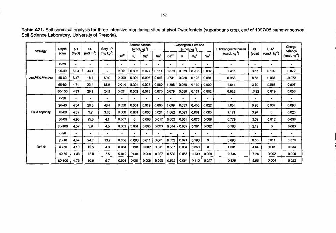
152

Table A21. Soil chemical analysis for three intensive monitoring sites at pivot Tweefontein (sugarbeans crop, end of 1997/98 summer season,Soil Science Laboratory, University of Pretoria).

Strategy

Leaching fraction

Field capacity

Deficit

Depth(cm)

0-20

20-40

40-60

60-80

80-100

0-20

20-40

40-60

60-80

80-100

0-20

20-40

40-60

60-80

80-100

PH(H2O)

-

5.04

8.47

4.71

4.53

-

4.54

4.32

4.96

4.52

-

4.84

4.10

4.43

4.73

EC(mS m*1)

-

44.1

18.4

23.4

28.1

-

28.5

3.7

15.8

5,9

-

24.7

15.6

13.0

10.8

Bray IP(mg kg"1)

-

-

50.0

86.5

24.9

-

48.4

3.85

4.1

4.0

-

13.7

4.3

7.5

6.7

Soluble cations(cmblc kg"1)

Ca2*

-

0.051

0.009

0.014

0.021

-

0.050

0.008

0.007

0.002

-

0.038

0.034

0.012

0.008

-

0.002

0.001

0.001

0.002

-

0.001

0.001

0

0.001

-

0.003

0.001

0.001

0.001

Mg34

-

0.027

0.005

0.008

0.018

-

0.019

0.006

0.006

0.003

-

0.011

0.002

0.008

0.008

Na*

-

0.111

0.043

0.060

0.073

-

0.088

0.021

0.017

0.003

-

0.061

0.011

0.027

0.025

Exchangeable cations(cmolokg'1)

Ca2t

-

0.579

0,731

1.385

0,679

-

1.099

1.062

0.663

0.374

-

0.632

0.587

0.539

0.622

K'

-

0.039

0.030

0.030

0.058

-

0.033

0.023

0.031

0.031

-

0.071

0.064

0.058

0.064

Mg2*

-

0.786

0.123

0.139

0.187

-

0.480

0.081

0.076

0,381

-

0.190

0.350

0.139

0.112

Na*

-

0.032

0.081

0.090

0,062

0.022

0.005

0.009

0.002

-

0

0

0.009

0.027

I echangeable bases(cmolc kg')

-

1.436

0.965

1.644

0.986

-

1.634

1.171

0.779

0.788

-

0.893

1.001

0.745

0.825

Cl"(ppm)

-

3.67

8.58

3.70

13.92

-

8.95

3.94

3.39

2.12

-

8.55

4.64

7.24

5.66

SO42"(cmoU kg"1)

-

0.109

0,035

0.066

0.019

-

0.037

0

0.012

0

-

0.011

0.001

0.002

0.004

Chargebalance

(cmolc kg"1)

-

0.072

-O.072

0.007

0.056

-

0.096

0.025

0.008

0.003

•

0.078

0.034

0.026

0.022

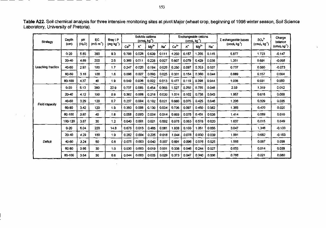
153

Table A22. Soil chemical analysis for three intensive monitoring sites at pivot Major (wheat crop, beginning of 1998 winter season, Soil ScienceLaboratory, University of Pretoria).

Strategy

Leaching fraction

Field capacity

Deficit

Depth(cm)

0-20

20-40

40-60

60-80

80-100

0-20

20-40

40-60

60-80

80-100

100-120

0-20

20-40

40-60

60-80

80-100

PH(H2O)

5.85

4.89

2.92

3.18

4.37

5.13

4.12

3.29

3.42

3.92

3.87

6.04

4.29

3.24

3.66

3.64

EC(mS m'1)

390

200

180

100

40

380

190

120

120

40

30

220

180

50

30

30

Bray IP

(mg kg1)

9.3

2.0

1.7

1.6

1.9

22.9

0.9

0.7

1.9

.1.6

1.2

14.8

1.9

0,8

1.0

0.6

Soluble cations{cmoU kg"1)

Ca2*

0.798

0.369

0.247

0.096

0.040

0.737

0.362

0.237

0.350

0.058

0.040

0.676

0.282

0.075

0.030

0.044

K*

0.028

0.011

0.020

0.027

0.006

0.085

0.008

0.004

0.006

0.003

0.001

0.013

0.004

0.003

0.003

0.003

Mga*

0.639

0.226

0.194

0.093

0.022

0.454

0.218

0.102

0.130

0.024

0.021

0.465

0.225

0.040

0.019

0.025

Na*

0.111

0.027

0.026

0.025

0.013

0.055

0.030

0.021

0.004

0.014

0.002

0.061

0.016

0.007

0.001

0.029

Exchangeable cations(cmolc kg"')

Ca2+

4.250

0.807

0.250

0.331

0.477

1.527

1.074

0.660

0.736

0.869

0.976

1.838

1.044

0.891

0.338

0.373

\C

0.157

0.079

0.097

0.154

0.119

0.250

0.102

0.075

0.097

0.078

0.063

0.103

0.078

0.096

0.046

0.047

Mg2*

1.355

0.429

0.353

0.360

0.398

0.765

0.738

0.425

0.450

0.431

0.578

1.051

0.830

0.576

0.244

0.340

Na*

0.115

0.036

0,037

0.044

0.044

0.048

0.043

0.046

0.082

0.036

0.020

0.055

0.039

0.025

0.027

0.006

1 echangeabie bases{cmolc kg1)

5.877

1.351

0.737

0.889

1.038

2.59

1.957

1.206

1.365

1.414

1.637

3.047

1.991

1.588

0.655

0.766

SO*3"(cmoiokg'1)

1.723

0.691

0.560

0.157

0.031

1.319

0.618

0.329

0.470

0.089

0.015

1.348

0.682

0.087

0.014

0.021

Chargebalance

(crrible kg*1)

-0.147

-0.058

-0.073

0.084

0.050

0.012

0.000

0.035

0.020

0.01O

0.049

-0.133

-0.153

0.038

0.039

0.080

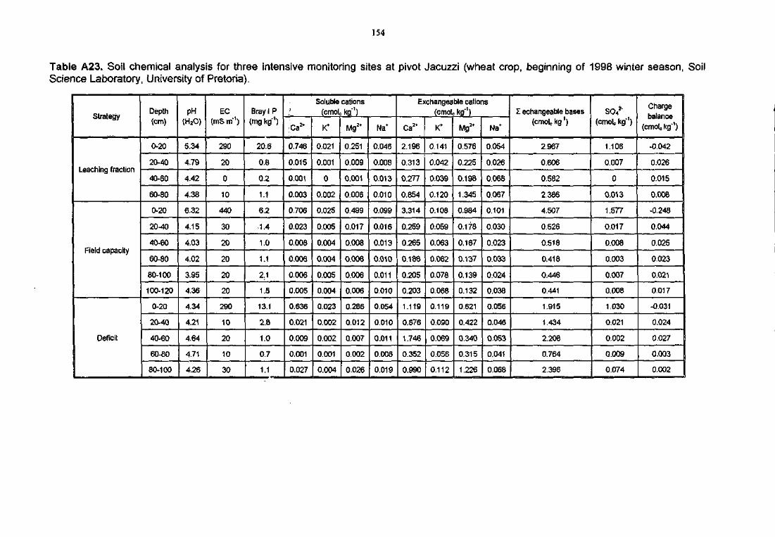
154

Table A23. Soil chemical analysis for three intensive monitoring sites at pivot Jacuzzi (wheat crop, beginning of 1998 winter season, SoilScience Laboratory, University of Pretoria).

Strategy

Leaching fraction

Field capacity

Deficit

Depth(cm)

0-20

20-40

40-60

60-80

0-20

20^0

40-60

60-80

80-100

100-120

0-20

20-40

40-60

60-80

80-100

pH(H2O)

5.34

4.79

4.42

4.38

6.32

4.15

4.03

4.02

3.95

4.36

4.34

4.21

4.64

4.71

4.26

EC(mS m'1)

290

20

0

10

440

30

20

20

20

20

290

10

20

10

30

Bray 1 P(mgkg1)

20,6

0.B

0.2

1.1

6.2

•1.4

1.0

1.1

2.1

1.5

13.1

2.a

1.0

0.7

1.1

Soluble cations.: (cmolc kg"1)

0.746

0.015

0.001

0.003

0.706

0.023

0.008

0.006

0.006

0.005

0.636

0.021

0.009

0.001

0.027

K*

0.021

0.001

0

0.002

0.025

0.005

0.004

0.004

0.005

0.004

0.023

0.002

0.002

0.001

0.004

Mg3*

0.251

0.009

0.001

0.006

0.499

0.017

0.008

0.006

0.006

0.006

0,286

0,012

0.007

0.002

0.026

Na*

0.046

0.008

0.013

0.010

0.099

0,016

0.013

0.010

0.011

0.010

0.054

O.010

0.011

0.008

0.019

Exchangeable cations(cmolc kg'1)

Ca3'

2.196

0.313

0.277

0.854

3.314

0.259

0.265

0.186

0.205

0.203

1.119

0.876

1.746

0.352

0.990

0.141

0.042

0.039

0.120

0.108

0.059

0.063

0.062

0.078

0.068

0.119

0.090

0.069

0.056

0.112

Mg3*

0.576

0.225

0.198

1.345

0.984

0.178

0.167

0.137

0.139

0.132

0.621

0.422

0.340

0.315

1.226

Na*

0.054

0.026

0.06B

0.067

0.101

0.030

0.023

0.033

0.024

0.038

0.056

0.046

0.053

0.041

0.068

Z echangeable bases(cmolc kg')

2.967

0.606

0.582

2386

4.507

0.526

0.518

0.418

0.446

0.441

1.915

1.434

2.208

0.764

2.396

SO-,1"(cmoU kg')

1.106

0.007

0

0.013

1.577

0.017

0.008

0.003

0.007

0.008

1.030

0.021

O.002

0.009

0.074

Chargebalance

(crnol,; kg"1)

-0.042

0.026

0,015

0.008

-0.246

0.044

0.025

0.023

0.021

0.017

-0.031

0.024

0.027

0.003

0.002

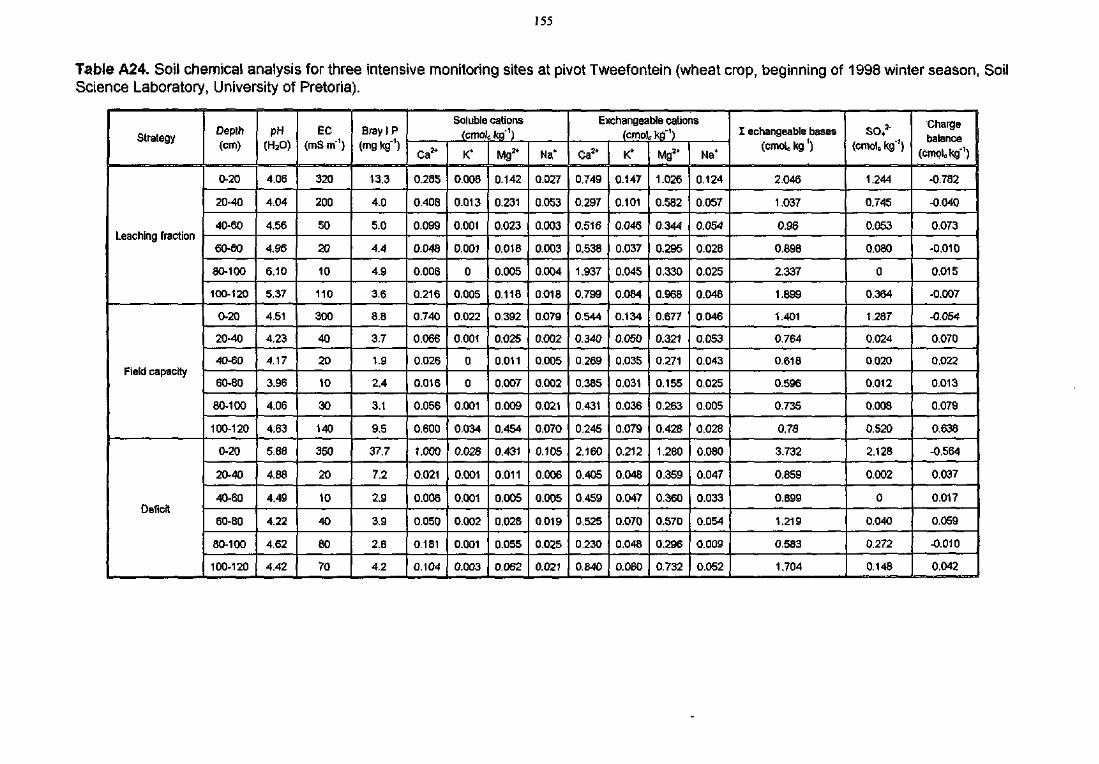
J55

Table A24. Soil chemical analysis for three intensive monitoring sites at pivot Tweefontein (wheat crop, beginning of 1998 winter season, SoilScience Laboratory, University of Pretoria).

Strategy

Leaching fraction

Field capacity

Deficit

Depth(cm)

0-20

20-40

40-60

60-eo

80-100

100-120

0-20

20-40

40-60

60-80

80-100

100-120

0-20

20-40

40-60

60-80

80-100

100-120

pH(HjO)

4.06

4.04

4.56

4.96

6.10

5.37

4.51

4.23

4.17

3.96

4.06

4.63

5.88

4.88

4.49

4.22

4.62

4.42

EC(mSm1)

320

200

50

20

10

110

300

40

20

10

30

140

350

20

10

40

80

70

Bray IP(mg kg'1)

13.3

4.0

5.0

4.4

4.9

3.6

8.8

3.7

1.9

2,4

3.1

9.5

37.7

7.2

2,9

3,9

2,8

4.2

Soluble cations(cwok kg'1)

Ca2*

0.285

0.408

0.099

0.048

0.006

0.216

0.740

0.066

0.026

0.016

0.056

0.600

1.000

0.021

0.006

0.050

0.181

0.104

K*

0.008

0.013

0.001

0.001

0

0.005

0.022

0.001

0

0

0.001

0.034

0.028

0.001

0.001

0.002

0.001

0.003

Mg**

0.142

0.231

0.023

0.018

0.005

0.118

0.392

0.025

0.011

0.007

0.009

0.454

0.431

0.011

0.005

0.028

0.055

0.062

Na*

0.027

0.053

0.003

0.003

0.004

0.016

0.079

0.002

0.005

0,002

0.021

0.070

0.105

0.006

0.005

0.019

0.025

0.021

Exchangeable cations(cmolc ksf1)

Ca*

0.749

0.297

0.516

0.538

1.937

0.799

0.544

0.340

0.269

0.385

0.431

0.245

2.160

0.405

0.459

0.525

0.230

0.840

K*

0.147

0.101

0.046

0.037

0.045

0.084

0.134

0.O50

0.035

0.031

0.036

0.079

0.212

0.048

0.047

0.070

0.048

0.080

Mg2t

1.026

0.582

0.344

0.295

0.330

0.968

0.677

0.321

0.271

0.155

0.263

0.428

1.260

0.359

0.360

0.S70

0.296

0.732

Na4

0.124

0.057

0.054

0.028

0.025

0.048

0.046

0.053

0.043

0.025

0.005

0.028

0.080

0.047

0.033

0.054

0.009

0.052

I echangeable bases(enrol, kg')

2.046

1.037

0.96

0.898

2.337

1.899

1.401

0.764

0.618

0.596

0.735

0.78

3.732

0.859

0.899

1.219

0.583

1.704

SO42-

(cmolckg-')

1.244

0.745

0.053

0.080

0

0.364

1.287

0.024

0.020

0.012

0.008

0.520

2.128

0.002

0

0.040

0.272

0.148

Chargebalance

(cmoUkg1)

-0.782

-0.040

0.073

-0.010

0.015

-0.007

-0.054

0.070

0.022

0.013

0.079

0.638

-0.564

0.037

0.017

0.059

-0.010

0.042

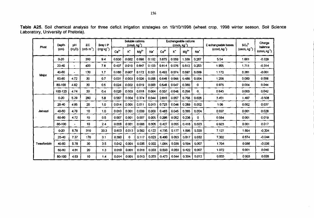
156

Table A25. Soil chemical analysis forLaboratory, University of Pretoria).

three deficit irrigation strategies on 19/10/1998 (wheat crop, 1998 winter season, Soil Science

Pivot

Major

Jacuzzi

Tweefontein

Depth(cm)

0-20

20-40

40-60

60-80

80-100

100-120

0-20

20-40

40-60

60-80

80-100

0-20

20-40

40-60

60-80

80-100

pH(HjO)

-

-

-

4.72

4.82

4.74

5.29

4.95

4.79

4.72

-

6.78

7.37

5.78

4.61

4.63

EC{mS m"1)

360

400

130

30

30

30

280

20

10

10

10

310

170

30

20

10

Bray 1 P(nig kg'1)

9.4

7.8

1.7

0.7

0.5

0.4

5.8

1.0

1.0

0.5

2.4

33.3

3.1

3.5

1.3

1.4

Soluble cations(cmolc kg"1)

Ca3t

0.530

0.437

0.160

0.031

0.024

0.020

0.567

0.014

0.010

0.007

0.006

0.603

0.390

0.042

0.019

0.014

K*

0.002

0.010

0.007

0.003

0.002

0.003

0.004

0.001

0.001

0.001

0.001

0.013

0

0.001

0.001

0,001

Mg2*

0,698

0.847

0.172

0.026

0.019

0.018

0.374

0.011

0.009

0.007

0.006

0.562

0.117

0.035

0,018

0,013

Na*

0.102

0.103

0.021

0.006

0.003

0.004

0.044

0-013

Q.009

0.005

0.005

0.122

0.023

0.002

0.003

0,003

Exchangeable cations(cmolc kg'1)

Ca*

3.875

0.814

0.492

0.646

0.548

0.337

2.610

0.723

0.483

0.296

0.427

4.735

6.400

1.064

0.593

0.473

K*

0.059

0.076

0.074

0.068

0.047

0.048

0.057

0.046

0.045

0,052

0.055

0.177

0.053

0.039

0.050

0.044

Mg2*

1,339

0.812

0.597

0.488

0,360

0,258

0.758

0.289

0.365

0.236

0.418

1.895

0.817

0.594

0.422

0.304

0.267

0.253

0.009

0.004

0

0.

0.026

0.002

0.004

0

0.023^

0.320

0.032

0.007

0.007

0.012

I echangeable bases(cmolc kg1)

5.54

1.955

1.172

1.206

0.975

0.643

3.451

1.06

0.897

0.584

0.923

7.127

7.302

1.704

1.072

0.833

SO4'"(cmole kg'1)

1.661

1.711

0.361

0.060

0.004

0.003

1.497

0.002

0.001

0.001

0.001

1.604

0.574

0.086

0.001

0.003

Chargebalance

(cmolo Kg*1)

-0.329

-0.314

-0.001

0.006

0.044

0.042

-0.508

0.037

0.028

0.019

0.017

-0.304

-0.044

-0.006

0.040

0.028

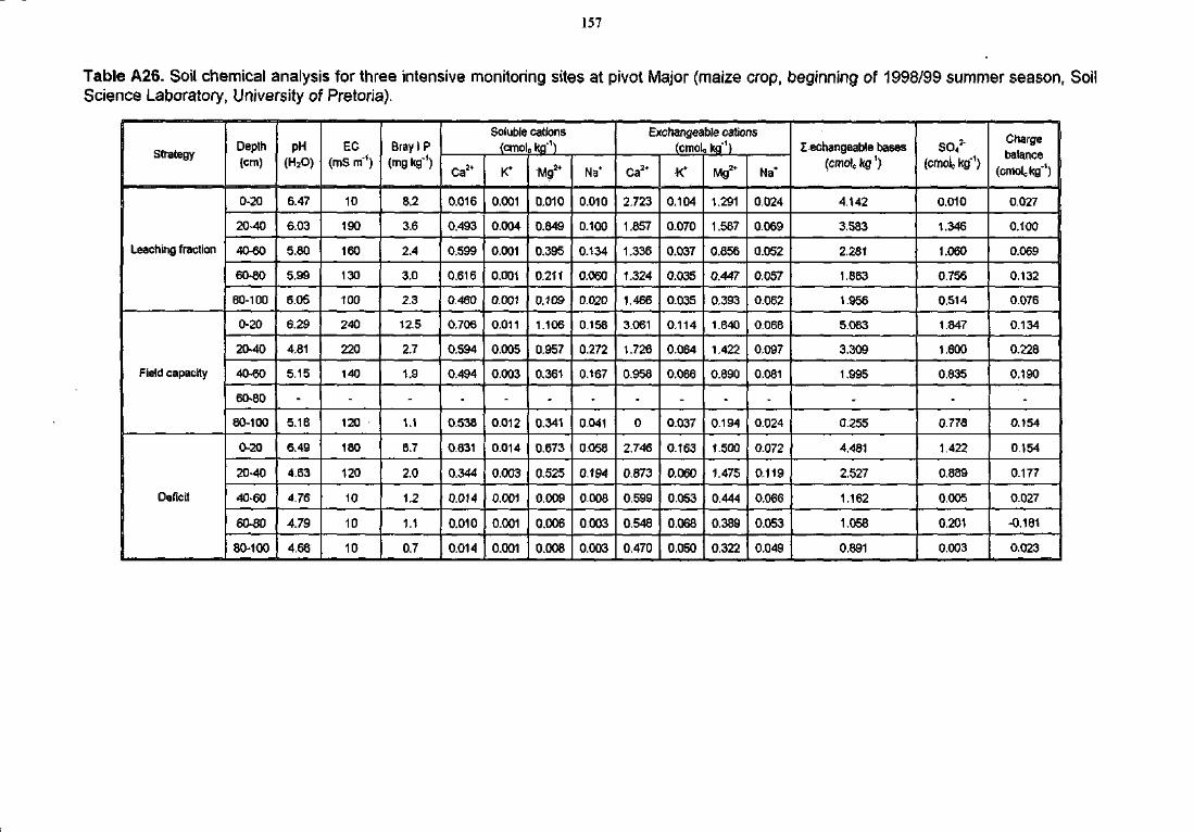
157

Table A26. Soil chemical analysis for three intensive monitoring sites at pivot Major (maize crop, beginning of 1998/99 summer season, SoilScience Laboratory, University of Pretoria).

Strategy

Leaching fraction

Field capacity

Deficit

Depth(cm)

0-20

20-40

40-60

60-80

80-100

0-20

20-40

40-60

60-80

80-100

0-20

20-40

40-60

60-80

80-100

pH(H2O)

6.47

6.03

5.80

5.99

6.05

6.29

4.81

5.15

-

5.16

6.49

4.63

4.76

4.79

4.66

EC(mS m"1)

10

190

160

130

100

240

220

140

-

120

180

120

10

10

10

Bray I P(mg kg1)

8.2

3.6

2.4

3.0

2.3

12.5

2.7

1.9

-

1.1

8.7

2.0

1.2

1.1

0.7

Soluble cations(cmolo kg"1)

Ca2*

0.016

0.493

0.599

0.616

0.460

0,706

0.594

0.494

-

0.538

0.831

0.344

0.014

0.010

0.014

K*

0.001

0.004

0.001

0.001

0.001

0.011

0.005

0.003

-

0.012

0.014

0.003

0.001

0.001

0.001

Mg2*

0.010

0.849

0.395

0.211

0.109

1.106

0.957

0.361

-

0.341

0.673

0.525

0.009

0.006

0.008

Na*

0.010

0.100

0.134

0.060

0.020

0.158

0.272

0.167

-

0.041

0.058

0.194

0,008

0.003

0.003

Exchangeable cations(cmol0 kg"1)

Ca2*

2.723

1.857

1.336

1.324

1.466

3.061

1.726

0.958

-

0

2.746

0.873

0.599

0.548

0.470

K*

0.104

0.070

0.037

0.035

0.035

0.114

0.064

0.066

-

0.037

0.163

0.060

0.053

0.068

0.050

Mg2*

1.291

1.587

0.856

0.447

0.393

1.640

1.422

0.890

-

0.194

1.500

1.475

0.444

0.389

0.322

Na*

0.024

0.069

0.052

0.057

0.062

0.068

0.097

0.081

-

0.024

0.072

0.119

0.066

0.053

0.049

I echangeable bases(OTIOIC kg1)

4.142

3.583

2.261

1.863

1.956

5.083

3.309

1.995

-

0.255

4.481

2.527

1.162

1.058

0.891

SO4!"

(cmoio kg"1)

0.010

1.346

1.060

0.756

0.514

1.847

1.600

0.835

-

0.778

1.422

0.889

0.005

0.201

0.003

Chargebalance

(cmolckg"')

0.027

0.100

0.069

0.132

0.076

0.134

0.228

0.190

-

0.154

0.154

0.177

0.027

-0.161

0.023

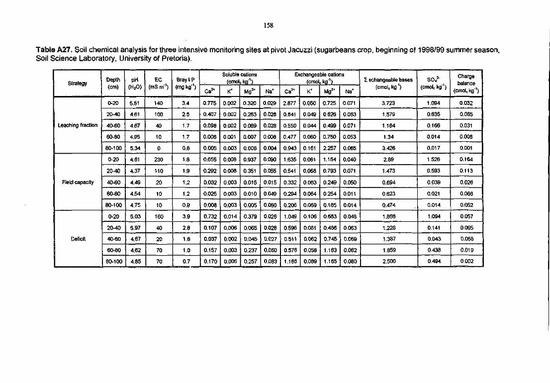
158

Table A27. Soil chemical analysis for three intensive monitoring sites at pivot Jacuzzi (sugarbeans crop, beginning of 1998/99 summer season,Soil Science Laboratory, University of Pretoria).

Strategy

Leaching fraction

Field capacity

Deficit

Depth(cm)

0-20

20-40

40-60

60-80

80-100

0-20

20-40

40-60

60-80

80-100

0-20

20-40

40-60

60-80

80-100

PH(HaO)

5.51

4.61

4.67

4.95

5.34

4.61

4.37

4.49

4.54

.4.75

5.03

5.97

4.67

4.62

4.85

EC(mS m'1)

140

100

40

10

0

230

110

20

10

10

160

40

20

70

70

Bray 1P(mg kg')

3.4

2.5

1.7

1.7

0.8

1.8

1.9

1.2

1.2

0.9

3.9

2.8

1.6

1.0

0.7

Soluble cations(cmolc kg"1)

Ga*

0.775

0.407

0.098

0.006

0.005

0.655

0.292

0.032

0.025

0.008

0.732

0.107

0.037

0.157

0.170

K*

0.002

0.002

0.002

0.001

0.003

0.008

0.008

0.003

0.003

0.003

0.014

0.006

0.002

0.003

0.006

Mg2*

0.320

0.263

0.069

0.007

0.006

0.937

0.351

0.015

0.010

0.005

0.379

0.065

0.045

0.237

0.257

Na*

0.029

0.028

0.028

0.008

0.004

0.090

0.055

0.015

0.049

0.Q50

0.026

0.028

0.027

0.060

0.063

Exchangeable cations(cmdlc kg*1)

Ca2*

2.877

0.841

0.550

0.477

0.943

1.635

0.541

0.332

0.294

0.206

1.049

0.596

0.511

0.576

1.166

K*

0.050

0.049

0.044

0.060

0.161

0.061

0.068

0.063

0.064

0.Q69

0.106

0.081

0.062

0.058

0.089

Mg2*

0.725

0.626

0.499

0.750

2.257

1.154

0.793

0.249

0.254

0.185

0.683

0.486

0.745

1.163

1.165

Na*

0.071

0.063

0.071

0.053

0.065

0.040

0.071

0.050

0.011

0.014

0.048

0.063

0.069

0.062

0.080

I echangeable bases(cmolc kg')

3.723

1.579

1.164

1.34

3.426

2.89

1.473

0.694

0.623

0.474

1.886

1.226

1.387

1.859

2.500

SO<2"(cmoU kg'1)

1.094

0.635

0.166

0.014

0.017

1.526

0.593

0.039

0.021

0.014

1.094

0.141

0.043

0.438

0.494

Chargebalance

(cmolc kg"1)

0.032

0.065

0.031

0.008

0.001

0.164

0.113

0.026

0.066

0.052

0.057

0.055

0.068

0.019

0.002

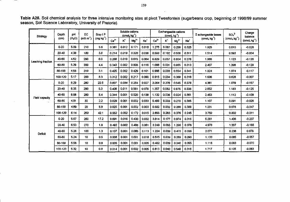
159

Table A28. Soil chemical analysis for three intensive monitoring sites at pivot Tweefontein (sugarbeans crop, beginning of 1998/99 summerseason, Soil Science Laboratory, University of Pretoria).

Strategy

Leaching fraction

Field capacity

Deficit

Depth(cm)

0-20

20-40

40-60

60-80

80-100

100-120

0-20

20-40

40-60

60-80

80-100

100-120

0-20

20-40

40-60

60-80

80-100

100-120

pH(HjO)

5.09

4.38

4.62

5.29

4.58

5.17

5.29

6.35

6.08

4.91

4.89

6.14

5.67

6.53

5.26

5.24

5.58

5.32

EC(mS nf1)

210

180

290

350

310

200

280

290

280

30

20

250

260

270

100

10

10

10

Bray I P(mg kg1)

5.6

3.8

6.0

4.4

3.1

8.3

22.5

5.3

5.4

2.2

5.9

42.1

17.2

1.8

1.3

0.5

0.8

0.8

Soluble cations(cmolc kg'1)

Ca2*

0.381

0.214

0.288

0.343

0.425

0.312

0.607

0.408

0.344

0.029

0.025

0.552

0,691

0.492

0.137

0.008

0.006

0.014

K*

0.012

0.019

0.010

0.002

0.002

0.002

0.034

0.011

0.001

0.001

0.001

0.052

0.016

0.002

0.001

0.001

0.001

0.001

Mg3t

0.171

0.320

0.615

0.808

0.429

0.217

0.254

0.561

0.520

0.002

0.002

0.172

0.430

0.486

0.065

0.001

0.001

0.002

Na*

0.018

0.036

0.084

0.116

0.101

0.090

0.027

0.078

0.138

0.033

0.003

0.015

0.032

0.061

0.113

0.018

0.005

0.005

Exchangeable cations(cmolc kg'1)

Ca*

1.275

0.593

0.829

1.098

0.996

0.915

3.064

1.357

1.132

0.499

0.602

2.855

3.814

3.249

1.224

0.515

0.482

0.813

K*

0.067

0.102

0.057

0.031

0.033

0.034

0.376

0.082

0.036

0.033

0.032

0.283

0.177

0.055

0.039

0.039

0.039

0.040

Mg2*

0.258

0.508

0.804

0.965

0.554

0.369

0.545

0.875

0.924

0.270

0.288

0.376

0.974

1.296

0.470

0.289

0.240

0.548

Na*

0.325

0.311

0.276

0.313

0.341

0.318

0.376

0.338

0.361

0.305

0.309

0.245

0.316

0.378

0.338

0.290

0.355

0.316

E echangeable bases(Gmo[c kg1)

1.925

1.514

1.966

2.407

1.924

1.636

4.361

2.652

2.453

1.107

1.231

3.759

5.281

4.978

2.071

1.133

1.116

1.717

SO42"

(cmolc kg"1)

0.610

0.593

1.123

1.398

1.074

0.628

1.079

1.183

1.112

0.091

0.078

0.802

1.406

1.207

0.238

0.085

0.083

0.105

Chargebalance

(cmole kg"1)

-0.028

-0.004

-0.126

-0.129

-0.117

-0.007

-0.157

-0.125

-0.109

-0.026

-0.047

-0.011

-0.237

-0.166

0.078

-0.057

-0.070

-0.083

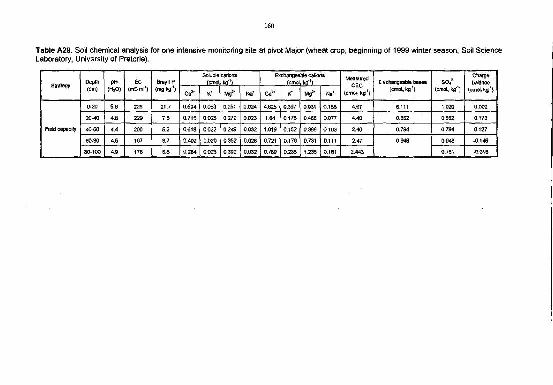
160

Table A29. Soil chemical analysis for one intensive monitoring site at pivot Major (wheat crop, beginning of 1999 winter season, Soil ScienceLaboratory, University of Pretoria).

Strategy

Field capacity

Depth(cm)

0-20

20-40

40-60

eo-Bo

80-100

pH(H2O)

5.6

4.8

4.4

4.5

4.9

EC(mS m"1)

226

229

200

167

176

Bray I P(mg Kg"1)

21.7

7.5

5.2

6.7

5.8

Soluble cations(cmoU kg'1)

0.694

0.715

0.618

0.402

0.264

0.053

0.025

0.022

0.020

0.025

Mg3*

0.251

0.272

0.249

0.352

0.392

Na*

0.024

0.023

0.032

0.028

0.032

Exchangeable cations(cmol6 kg'1)

| CaJt

4.625

1.64

1.019

0.721

0.789

0.397

0.176

0.152

0.176

0.238

Mg24

0.931

0.466

0.398

0.731

1.235

Na*

0,158

0.077

0.103

0.111

0.181

MeasuredCEC

(cmoUkg'1)

4.67

4.40

2.40

2.47

2.443

I echangeable bases(cmolckg1)

6.111

0.862

0.794

0.948

SO,!"(cmoic kg"1)

1.020

0.862

0.794

0.948

0.751

Chargebalance

(cmoUkg"1)

0.002

0.173

0.127

-0.146

-0.018

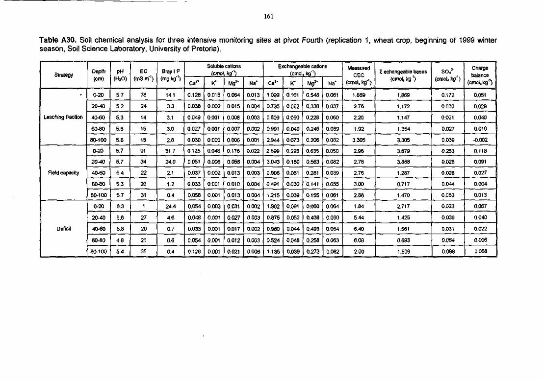
161

Table A30. Soil chemical analysis for three intensive monitoring sites at pivot Fourth (replication 1, wheat crop, beginning of 1999 winterseason, Soil Science Laboratory, University of Pretoria).

Strategy

Leaching fraction

Field capacity

Deficit

Depth(cm)

0-20

20-40

40-60

60-80

80-100

0-20

20-40

40-60

60-80

80-100

0-20

20-40

40-60

60-80

80-100

pH<H2O)

5.7

5.2

5.3

5.8

5.8

5.7

5.7

5.4

5.3

5.7

6.3

5.6

5.8

4.8

5.4

EC(mS m"1)

78

24

14

15

15

91

34

22

20

31

1

27

20

21

35

BraylP(mg kg'1)

14.1

3.3

3.1

3.0

2.8

31.7

24.0

2.1

1.2

0.4

24.4

4.6

0.7

0.6

0.4

Soluble cations(cmolckg1)

Ca*

0.128

0.038

0.049

0.027

0.030

0.125

0.051

0.037

0.033

0.058

0.054

0.048

0.033

0.054

0.128

K*

0.018

0.002

0.001

0.001

0.000

0.048

0.008

0.002

0.001

0.001

0.003

O.001

0.001

0.001

0.001

MB*

0.064

0.015

0.008

0.007

0.006

0.176

0.056

0.013

0.010

0.013

0.031

0.027

0.017

0.012

0.021

Na*

0.013

0.004

0.003

0.002

0.001

0.022

0.004

0.003

0.004

0.004

0.002

0.003

0.002

0.003

0.006

Exchangeable cations

(cmole kg1)

CaJt

1.099

0.735

0.809

0.991

2.944

2.899

3.043

0.906

0.491

1.215

1.902

0.875

0.960

0.S24

1.135

K*

0.161

0.062

iO050

0.049

0.073

0.295

0.180

0.0S1

0.030

0.039

0.091

0.052

0.044

0.048

0.039

Mg3*

0.548

0.338

0.228

0.245

0.206

0.635

0.563

0.281

0.141

0.155

0.660

0.438

0.493

0.258

0.273

Na*

0.061

0.O37

0.060

0.069

0.082

0.05O

0.082

0.039

0.055

0.061

0.064

0.060

0.064

0.063

0.062

MeasuredCEC

(cmolc kg"1)

1.869

2.76

2.20

1.92

3.305

2.96

2.76

2.76

3.00

2.86

1.84

5.44

6.40

6.08

2.00

I echangeable bases(cmolc kg*)

1.869

1.172

1.147

1.354

3.305

3.879

3.868

1.287

0.717

1.470

2.717

1.425

1.561

0.693

1.509

SO«*(cmolc kg'1)

0.172

0.030

0.021

0.027

0.039

0.253

0.028

0,028

0.044

0.063

0.023

0.039

0.031

0.064

0.098

Chargebalance

(cnwickg1')

0.051

0.029

0.040

0.010

-0.002

0.118

0.091

0.027

0.004

0.013

0.067

0.040

0.022

0.006

0.058

162

Table A30 (continued). Soil chemical analysis forwinter season, Soil Science Laboratory, University

three intensive monitoring sites at pivot Fourth (replication 2, wheat crop, beginning of 1999of Pretoria).

Strategy

Leaching fraction

Field capacity

Deficit

Depth(cm)

0-20

20-40

40-60

60-80

80-100

0-20

20-40

40-60

60-80

80-100

0-20

20-40

40-60

60-80

80-100

PH(HaO)

5.5

5.4

S.3

5.6

5.9

5.7

5.8

5.2

5.3

5.8

5.7

4.9

5.1

5.5

5.4

EC(mS m'1)

127

53

31

30

19

123

20

15

17

21

143

91

24

28

17

Bray i P(mg kg1)

25.3

5.3

3.9

6.4

4.8

20.8

6.5

5.4

4.5

3.5

13.8

4.8

4.2

6.1

4.8

Soluble cations.. r.cmolc kg"1)

Ca!*

0331

0.103

0.064

0.072

0.041

0.240

0.027

0.022

0.023

0.042

0.313

0.203

0.040

0.059

0.030

K*

0.017

0.003

0.001

0.001

0.001

0.026

0.001

0.001

0.002

0.001

0.045

0.011

0.002

0.002

0.002

Mg3*

0.171

0.064

0.029

0.015

0.012

0.154

0.026

0.016

0.012

0.014

0.169

0.111

0.029

0.016

0.012

Na*

0.033

0.007

0.000

0.000

0.000

0.029

0.000

0.000

0.000

0.000

0.032

0.020

0.002

0.005

0.001

Exchangeable cations(cmole kg?1)

ca*

1.231

0.835

0.640

0.9B1

1.821

1.267

1.130

0.532

0.920

1.345

1.458

2.766

0.713

1.189

1.038

\C

0.171

0.083

0.064

0.072

0.068

0.255

0.083

0.081

0.091

0.090

0.316

0.172

0.101

0.107

0.104

Mg1 ' :

0.841

0.510

0.323

0.3O2

0.288

0.908

0.629

0.367

0.339

0.287

0.807

0.602

0.396

0.285

0.322

Na*

0.093

0.070

0.040

0.064

0.076

0.101

0.108

0.239

0.147

0.165

0.116

0.123

0.063

0.116

0.094

MeasuredCEC

(cmolc kg'1)

2.88

2.60

2.36

2.44

3.32

3.16

3.44

2.84

3.53

2.33

3.73

3.07

2.33

2.27

2.93

I echangeable bases(cmoU kg')

2.336

1.498

1.067

1.419

2.253

2.531

1.950

1.219

1.497

1.887

2.697

3.663

1.273

1.697

1.558

SO<J"(omoU kg1)

0.471

0.155

0.039

0.045

0.053

0.546

0.055

0,050

0.043

0.057

0.403

0.227

0.020

0.046

0.037

Chargebalance

(cmolc kg"1)

0.0B1

0.022

0.055

0.043

0.001

-0.097

-0.001

-0.011

-0.006

0.000

0.156

0.118

0.053

0.036

0.008

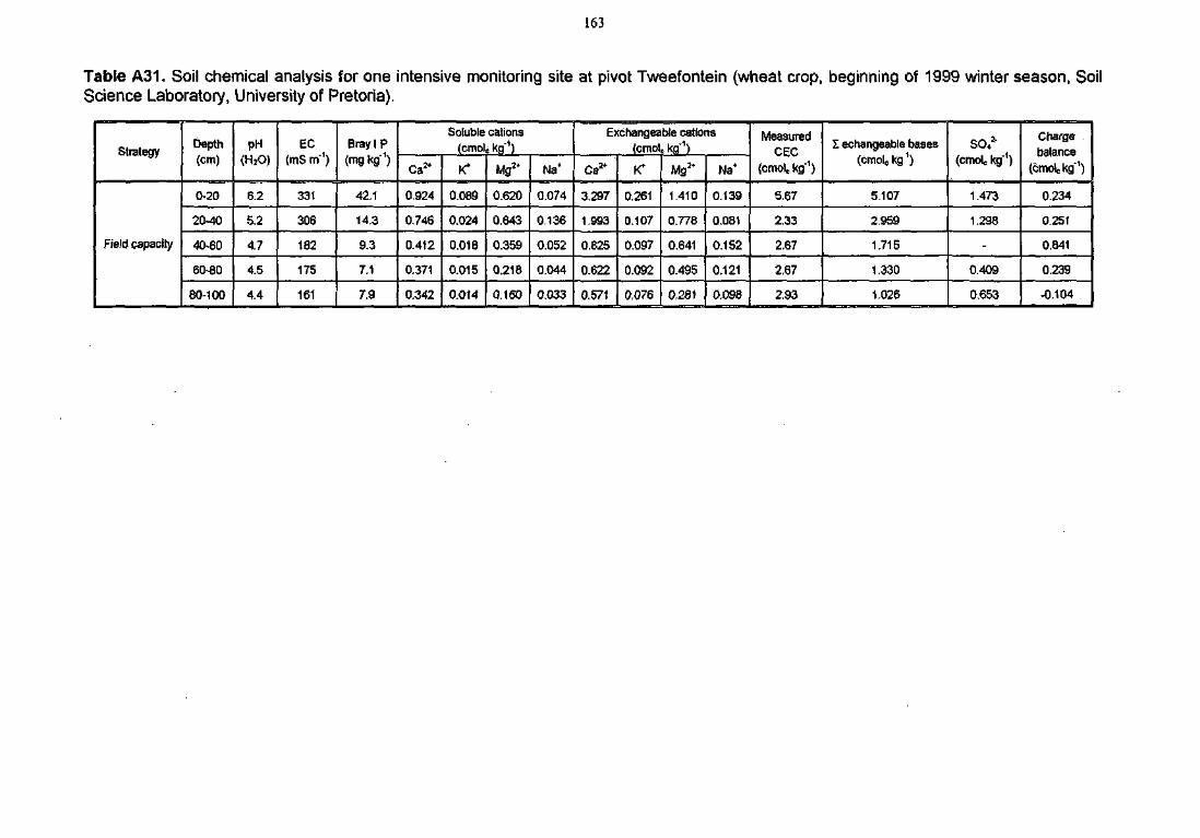
163

Table A31. Soil chemical analysis for one intensive monitoring site at pivot Tweefontein (wheat crop, beginning of 1999 winter season, SoilScience Laboratory, University of Pretoria).

Strategy

Field capacity

Depth(cm)

0-20

20-40

40-60

60-80

80-100

PH(HaO)

6.2

5.2

4.7

4.5

4.4

EC(mS m"1)

331

306

182

175

161

Bray IP{mg kg 1)

42.1

14.3

9.3

7.1

7.9

Soluble cations(cmolc kg'1)

Ca3*

0.924

0.746

0.412

0.371

0.342

K*

0.089

0.024

0.018

0.015

0.014

Mg3*

0.620

0.643

0,359

0.218

0.160

Naf

0.074

0.136

0.052

0.044

0.033

Exchangeable cations(cmolc kg"1)

Ca3*

3.297

1.993

0.825

0.622

0.571

0.261

0.107

0.097

0.092

0.076

Mg3*

1.410

0.778

0.641

0.495

0.281

Na*

0.139

0.081

0.152

0.121

0.098

MeasuredCEC

(cmolc kg'1)

5.67

2.33

2.67

2.67

2.93

I eohangeable bases

(cmolc kg')

5.107

2.959

1.715

1.330

1.026

SO,*(cmolc kg"1)

1.473

1.298

-

0.409

0.653

Chargebalance

(cmolc kg*1)

0.234

0.251

0.841

0.239

-0.104

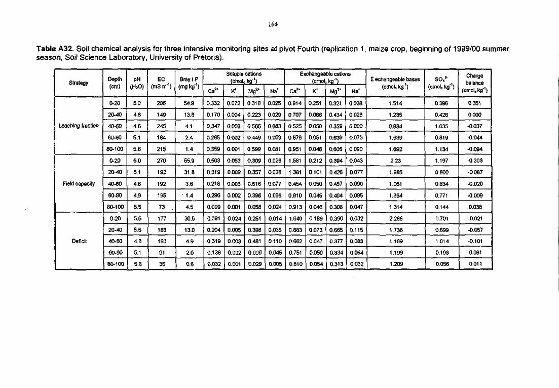
164

Table A32. Soil chemical analysis for three intensive monitoring sites at pivot Fourth (replication 1, maize crop, beginning of 1999/00 summerseason, Soil Science Laboratory, University of Pretoria).

Strategy

Leaching fraction

Field capacity

Deficit

Depth(cm)

0-20

20-40

40-60

60-80

80-100

0-20

2D-40

40-60

60-80

80-100

0-20

20-40

40-60

60-80

80-100

pH

(HiO)

5.0

4.8

4.6

5.1

5.6

5.0

5.1

4.6

4.9

5.5

5.6

5.5

4.8

5.1

5.6

EC<mS m"1)

206

149

245

184

215

270

192

192

195

73

177

183

193

91

35

Brayi P

(mg kg1 )

54.9

13.0

4.1

2.4

1.4

55.9

31.8

3.6

1.4

4.5

30.5

13.0

4.9

2.0

0.6

Soluble cations

(crnole kg"1)

Ca24

0.332

0.170

0.347

0.265

0.359

0.503

0.319

0.218

0.296

0.099

0.391

0.204

0.319

0.136

0.032

K>

0.072

0.004

0.003

0.002

0.001

0,053

0.009

O.003

0.002

0.001

0.024

0.005

0.003

0.002

0.0O1

Mg2*

0.318

0.223

0.565

0.449

0.599

0.309

0.357

0.516

0.396

0.058

0.251

0.398

0.481

0.096

0.029

Na*

0.025

0.029

0.083

0.059

0.081

0.026

0.028

0.077

0.068

0.024

O.014

0.035

0.110

0.045

0.005

Exchangeable cations(cmolokg'1)

Ca3*

0.914

0.707

0.525

0.876

0.951

1.581

1.381

0.454

0.810

0.913

1,649

0.883

0.662

0.751

0.810

K*

0.251

0.066

0.050

0.051

0.046

0.212

0.101

0.O50

0.045

0.046

0.189

0.073

0.047

0.050

0.054

Mg-

0.321

0.434

0.359

0.639

0.605

0.394

0.426

0.457

0.404

0.308

0.396

0.665

0.377

0.334

0.313

Na*

0.028

0.028

0.000

0,073

0.090

0.043

0.077

0.090

0.095

0.047

0.032

0.115

0.083

0.064

0,032

I echangeable bases(ctnolc kg1)

1.514

1.235

0.934

1.639

1.692

2.23

1.985

1.051

1.354

1.314

2.266

1.736

1.169

1.199

1.209

SO,2"(omolc kg"1)

0.396

0.426

1.035

0.819

1.134

1.197

0.800

0.834

0.771

0.144

0.701

0.699

1.014

0.198

0.056

Chargebalance

(cmoUkg1)

0.351

0.000

-0.037

-0.044

-0.094

-0.306

-0.087

-0.020

-0.009

0.038

-0,021

-0.057

-0.101

0.081

0.011

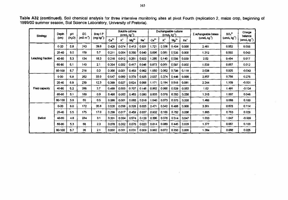
165

Table A32 (continued). Soil chemical analysis for three intensive monitoring sites at pivot Fourth (replication 2, maize crop, beginning of1999/00 summer season, Soil Science Laboratory, University of Pretoria).

Strategy

Leaching fraction

Field capacity

Deficit

Depth(cm)

0-20

20-40

40-60

60-80

80-100

0-20

20-40

40-60

60-80

80-100

0-20

20-40

40-60

60-80

80-100

PH<H2O)

5.9

5.0

5.3

5.1

5.7

5.8

5.9

5.2

5.1

5.8

6.0

5.5

4.8

5.3

5.7

EC(mS m'1)

243

159

134

143

216

262

230

286

189

60

172

175

234

68

36

Bray I P(mg kg1)

29.8

5.7

18.3

2.1

0.3

33.0

12.3

3.7

0.9

0.5

35.8

17.0

3.1

2.3

2.1

Soluble cations(cmolc kg1)

Ca2*

0,429

0.211

0.216

0.204

0.356

0.547

0.399

0.499

0.488

0.086

0.526

0.299

0.331

0.078

0.050

K*

0,074

0.004

0.012

0.002

0.001

0.080

0.027

0.003

0.002

0.001

0.058

0.017

0.004

0.002

0.001

Mg*

0.413

0.380

0.261

0.417

0.463

0.379

0.624

0.707

0.483

0.065

0.328

0.459

0.574

0.070

0.031

Na*

0.031

0.040

0.022

0.046

0,062

0.025

0.058

0.148

0.080

0.016

0.025

0.037

0.129

0.020

0.009

Exchangeable cations(cmol0 kg'1)

Ca2t

1.721

0.696

1.285

0.873

1.050

2.037

1.171

0.962

0.833

1.040

2.471

0.932

0.396

0.814

0.962

K*

0.336

0.081

0.140

0.061

0.062

0.374

0.194

O.066

0.076

0.073

0.342

0.165

0.076

0.089

0.072

Mg2*

0.404

0535

0.556

0.S97

0.798

0.446

0.818

0.529

0.350

0.375

0.488

0,752

0.514

0.445

0.350

Na*

0.000

0.000

0.039

0.002

0.118

0.000

0.061

0.063

0.056

0.000

0.000

0.036

0.047

0,029

0.000

I echangeable bases(cmolc kg')

2.461

1.312

2.02

1.533

2.028

2.857

2.244

1.62

1.315

1.488

3.301

1.865

1.033

1.377

1.384

SO,*(cmols kg"1)

0.852

0.592

0.494

0.657

0.925

0.756

1.109

1.491

1.007

0.068

0.823

0.783

1.047

0.067

0.066

Chargebalance

(cmolckg*1)

0.095

0.043

0.017

0.012

-0.043

0.275

-0.001

-0.134

0.046

0.1O0

0.114

0.029

-0.009

0.103

0.025

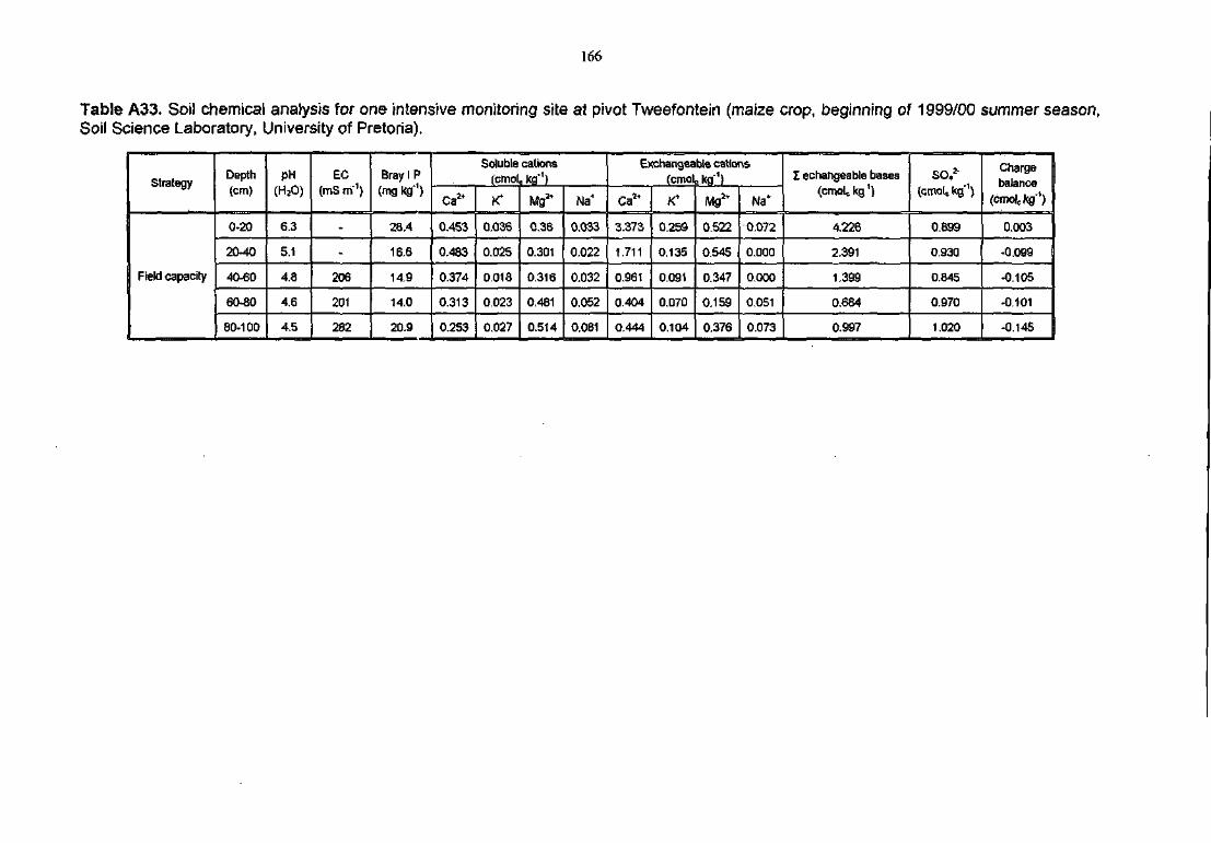
166

Table A33. Soil chemical analysis for one intensive monitoring site at pivot Tweefontein (maize crop, beginning of 1999/00 summer season,Soil Science Laboratory, University of Pretoria).

Strategy

Field capacity

Depth(cm)

0-20

20-40

40-60

60-80

80-100

PH(HaO)

6,3

5.1

4.8

4.6

4.5

EC(mS m"1)

-

-

206

201

282

Bray I P(mg kg')

28,4

16.6

14.9

14.0

20.9

Soluble cations(cmole Kg'1)

Ca*

0.453

0.483

0.374

0,313

0.253

K*

0.036

0.025

0.018

0.023

0.027

Mg1*

0.3S

0.301

0.316

0.481

0.514

Na1

0.033

0.022

0.032

0.052

0.081

Exchangeable cations(cmolekg")

Ca"

2.373

1.711

0.961

0.404

0.444

K*

0.259

0.135

0.091

0.070

0.104

• M g *

0.522

0.545

0.347

0.159

0.376

Na*

0.072

0.000

0.000

0.051

0.073

I echangeable bases(cmolckg1)

4.226

2.391

1.399

0.684

0.997

SO,2"(cmottkg'1)

0.899

0.930

0.845

0.970

1.020

Chargebalance

(bmolc kg"')

0.003

-0.099

-0.105

-0.101

-0.145

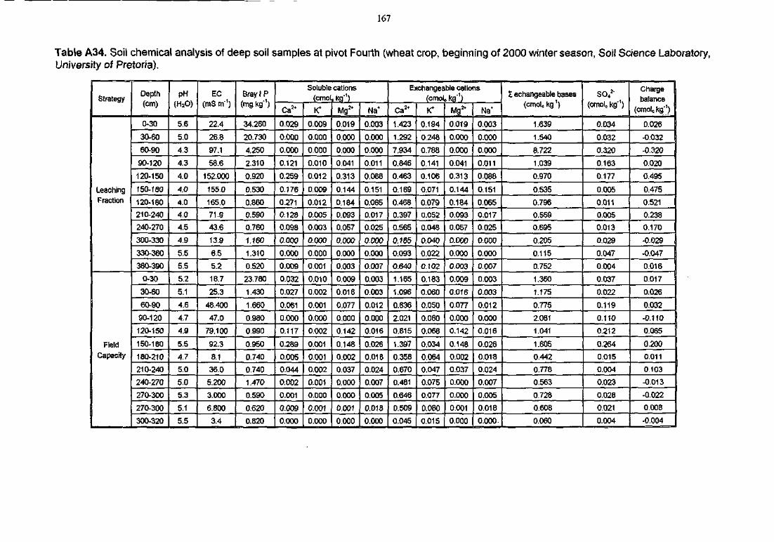
167

Table A34. Soil chemical analysis of deep soil samples at pivot Fourth (wheat crop, beginning of 2000 winter season, Soil Science Laboratory,University of Pretoria).

Strategy

LeachingFraction

FieldCapacity

Depth(cm)

0-30

30-60

60-90

90-120

120-150

150-130

120-180

210-240

240-270

300-330

330-360

360-390

0-30

30-60

60-90

90-120

120-150

150-180

180-210

210-240

240-270

270-300

270-300

300-320

PH<H2O)

5.6

5.0

4.3

4.3

4.0

4.0

4.0

4.0

4.5

4.9

5.5

5.5

5.2

5.1

4.6

4.7

4.9

5.5

4.7

5.0

5.0

5.3

5.1

5.5

EC(mS m'1)

22.4

26.8

97.1

58.6

152.000

155.0

165,0

71.9

43.6

13.9

6.5

5.2

18.7

25.3

48.400

47.0

79.100

92.3

8.1

36.0

5.200

3.000

6.800

3.4

Bray 1 PCmgkg1)

34.260

20.730

4.250

2.310

0.920

0.530

0.860

0.590

0.760

1.160

1.310

0.520

23.780

1.430

1.660

0.980

0.990

0.950

0.740

0.740

1.470

0.590

0.620

0.820

Soluble cations(cmote kg"')

0.029

0.000

0.000

0.121

0.259

0.176

0.271

0.128

0.098

0.000

0.000

0.009

0.032

0.027

0.061

0.000

0.117

0.289

0.005

0.044

0.002

0.001

0.009

0.000

K*

0.009

0.000

0.000

0.010

0.012

0.009

0.012

0.005

0.003

0.000

0.000

0.001

0.010

0.002

0.001

0.000

0.002

0,001

0.001

0.002

0.001

0.000

0.O01

0.000

Mgs*

0.019

L o.ooo0.000

0.041

0,313

0.144

0.184

0.093

0.057

0.000

0.000

0,003

0.009

0.016

0.077

0.000

0.142

0.148

0.002

0.037

O.OOO

0.000

0.001

0.000

Na*

0.003

0.000

0.000

0.011

0.088

0.151

0.065

0.017

0.025

0.000

0.000

0.007

0.003

0.003

0.012

0.000

0.016

0.026

0.018

0.024

0.007

0.005

0,018

0.000

Exchangeable cations(emole kg"1)

Ca*

1.423

1.292

7.934

0.846

0.463

0.169

0.468

0.397

0.565

0.165

0.093

0.640

1.165

1.096

0.636

2.021

0.815

1.397

0.358

0.670

0.481

0.646

0.509

0.045

K*

0.194

0.248

0.788

0.141

0.106

0.071

0.079

0.052

0.048

0.040

0.022

0.102

0.183

0.060

0.050

0.060

0.068

0.034

0.064

0.047

0.075

0.077

0.080

0.015

MgJ*

0.019

0.000

0.000

0.041

0.313

0.144

0.184

0.093

0.057

0.000

0.000

0.O03

0.009

0.016

0.077

0.000

0.142

0.148

0.002

0.037

0.000

O.OOO

0.001

0.000

Na*

0.003

0.000

0.000

0.011

0.088

0.151

0,065

0.017

0.025

0.000

0.000

0.007

0.003

0.003

0.012

0.000

0.016

0.026

0.018

0.024

0.007

0.005

0.018

0.000.

t echangeable bases(cmolc k g ' )

1.639

1.540

8.722

1.039

0.970

0.535

0.796

0.559

0.695

0.205

0.115

0.752

1.360

1.175

0.775

2.081

1.041

1.605

0.442

0.778

0.563

0.728

0.608

0.060

SO42"

(cmolckg !)

0.034

0.032

0.320

0.163

0.177

0.005

0,011

0.005

0.013

0.029

0.047

0.004

0.037

0.022

0.119

0.110

0.212

0.264

0.015

0.004

0.023

0.028

0.021

0.004

Chargebalance

(cmolckg"1)

0.026

-0.032

-0.320

0.020

0.495

0.475

0.521

0.238

0.170

-0,029

-0.047

0.016

0.017

0.026

0.032

-0.110

0.Q65

0.200

0.011

0.103

-0.013

-0.022

0.008

-0.004

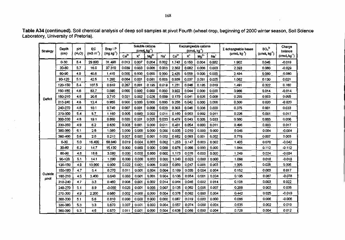
168

Table A34 (continued). Soil chemical analysis of deep soil samples at pivot Fourth (wheat crop, beginning of 2000 winter season, Soil ScienceLaboratory, University of Pretoria).

Strategy

Deficit

Outsidepivot

Depth(cm)

0-30

30-60

60-90

90-120

120-150

150-180

180-210

210-240

240-270

270-300

300-330

330-360

360-380

380-400

0-30

30-60

60-90

90-120

120-150

150-180

180-210

210-240

240-270

270-300

300-330

330-360

360-390

PH(HJOJ

5.4

5.7

4.9

5.1

5.4

4.6

4.6

4.8

4.8

5.4

4.8

4.9

6.1

5.6

5.0

6.2

4.8

5.1

4.9

4,74.5

4.7

5.1

4.9

5.1

5.3

5.3

EC(mS m"')

29.800

16.0

40.8

42.5

107.5

83.7

20.8

12.4

10.1

5.7

19.1

6.2

2,6

2,0

16.400

14.7

18.8

14.1

13.900

5,4

3.400

3.3

8.9

2.200

5.6

3.3

4.6

Bray I P(mg kg1)

31.490

37.310

1.410

1.260

0.610

0.590

0.710

0.950

0.740

1.160

0.660

0.630

1.060

0.210

58.040

15.130

3.080

1.090

0.900

0.270

0.640

0.460

-0.050

0.560

0.810

0.670

0.570

Soluble(enrol

Ca*

0.013

0.039

0.000

0.064

0.267

0.000

0.021

0.000

0.007

0.005

0.020

0.008

0.000

0.007

0.019

0.000

0.000

0.000

0.022

0.011

0.003

0.008

0.025

0.002

0,000

0.007

0.011

K*

0.007

0.003

0.000

0.001

0.001

0.000

0.002

0.000

0.001

0.000

0.001

0.001

0.000

0.000

0.004

O.Q00

0.000

0.000

0.001

0.001

0.001

0.001

0.001

0.000

0,000

0.001

0.001

cations

to"1)Mg1*

0.004

0.006

0.000

0.081

0.195

0.000

0.026

0.000

0.006

0.002

0.005

0.000

0.000

0.001

0.003

0.000

0.000

0.000

0.005

0.004

0.001

0.002

0.005

0.000

0.000

0.000

0.000

Na*

0.002

0.003

0.000

0.005

0.019

0.000

0.009

0.000

0.020

0.011

0.033

0.011

0.000

0.002

0.002

0,000

0.000

0.000

0.003

0.004

0.004

0.014

0.007

0,004

0,000

0.004

0.004

Exchangeable cations

(cmolckg"1)

Ca14

1.743

2.302

2.435

0.939

1.231

3.922

0.179

0.258

0.303

0.160

0,479

0.431

0.035

0.682

1.253

0.978

1.173

1.043

0.950

0.109

0.136

0.044

0.135

0.376

0.067

0.557

0.638

K*

0.153

0.082

0.059

0.037

0.046

0.044

0.041

0.042

0.046

0.053

0.043

0.054

0.010

0.093

0.147

0.066

0.076

0.023

0.047

0.035

0.054

0.046

0.062

0.062

0.019

0.074

0.086

0.004

0.006

0.000

0.081

0.195

0.000

0.026

0.000

0.006

0.002

0.005

0.000

0.000

0.001

0.003

0.000

0,000

0.000

0.005

0.004

0.001

0.002

0.005

0.000

0.000

0.000

0.000

Nav

0.002

0.003

0.000

0.005

0.019

0.000

0.009

0.000

0.020

0.011

0,033

0.011

0.000

0.002

0.002

0.000

0.000

0.000

0.003

0.004

0.004

0,014

0,007

0.004

0.000

0.004

0.004

I echangeable bases

(cmolc kg ' )

1.902

2.393

2.494

1.062

1.491

3.966

0.255

0.300

0.375

0.226

0.560

0.496

0.045

0.778

1.405

1.044

1.249

1.066

1.005

0.152

0.195

0.106

0.209

0.442

0,086

0.635

0.728

SO,5"

(cmoug1)

0.045

0.080

0.080

0.130

0.322

0.014

0.003

0.020

0.001

0.001

0.003

0.003

0.004

0.007

0.070

0.112

0.024

0.018

0.025

0.003

0.087

0.003

0.003

0.025

0.006

0.002

0,004

Chargebalance

(cmol0 kg"1)

-0.019

-0.029

-0.060

0.021

0.160

-0.014

0.055

-0.020

0.033

0.017

0.056

0.017

-0.004

0.003

-0.042

-0.112

-0.024

-0.018

0.006

0.017

-0.078

0.022

0.035

-0.019

-0.006

0.010

0.012

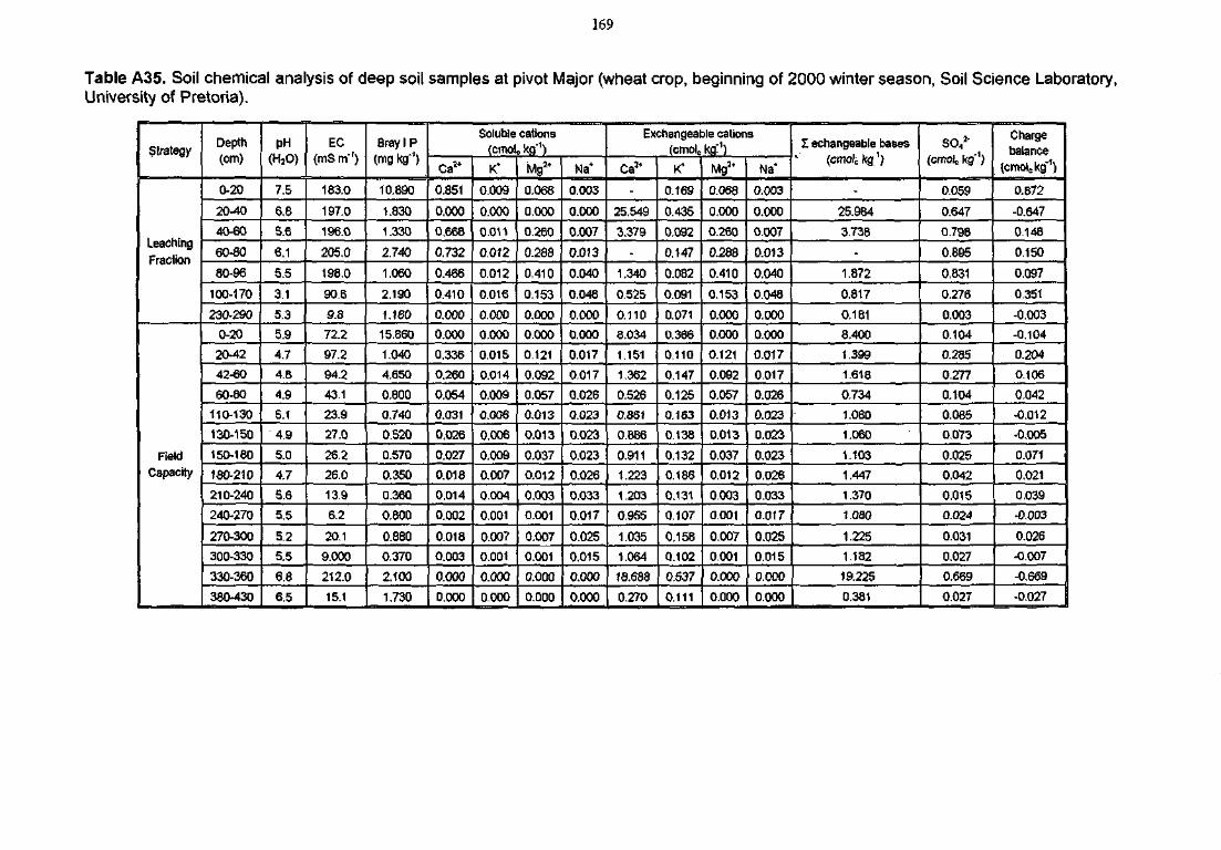
169

Table A35. Soil chemical analysis of deep soil samples at pivot Major (wheat crop, beginning of 2000 winter season, Soil Science Laboratory,University of Pretoria).

Strategy

LeachingFraction

FieldCapacity

Depth(cm)

0-20

20-40

40-60

60-80

80-96

100-170

230-290

0-20

20-42

42-60

60-80

110-130

130-150

150-180

180-210

210-240

240-270

270-300

300-330

330-360

380-430

PH(HSO)

7.5

6.8

5.6

6.1

5.5

3.1

5.3

5.9

4.7

4.8

4.9

5.1

4.9

5.0

4.7

5.6

5.5

5.2

5.5

6.8 I

6.5

EC<mS m"')

183.0

197.0

196.0

205.0

198.0

90.6

9.8

72.2

97.2

94.2

43.1

23.9

27.0

26.2

26.0

13.9

6.2

20.1

9.000

212.0

15.1

Bray IP(mg kg')

10.890

1.830

1.330

2.740

1.060

2.190

1.160

15.860

1.040

4.650

0.600

0.740

0.520

0.570

0.350

0.360

0.800

0.880

0.370

2.100

1.730

Soluble cations(cmolc kg"1)

Ca2*

0.851

0.000

0.668

0.732

0.466

0.410

0.000

0.000

0.336

0.260

0.054

0.031

0.026

0.027

0.018

0,014

0.002

0.018

0.003

0.000

0.000

K*

0.009

0.000

0.011

0.012

0.012

0.016

0.000

0.000

0.015

0.014

0.009

0.006

0.006

0.009

0.007

0.004

0.001

0.007

0.001

0.000

0.000

Mg2*

0.068

0.000

0.260

0.283

0.410

0.153

O.ODD

0.000

0.121

0.092

0.057

0.013

0.013

0.037

0.012

0.003

0.001

0.007

0.001

0.000

0.000

Na+

0.003

0.000

0.007

0.013

0.040

0.048

0.000

0.000

0.017

0.017

0.026

0.023

0.023

0.023

0.026

0.033

0.017

0.025

0.015

0.000

0.000

Exchangeable cations(cmolc kg:1)

-

25.549

3.379

-

1.340

0.525

0.110

6.034

1.151

1.362

0.526

0.861

0.886

0.911

1.223

1.203

0.955

1.035

1.064

16.688

0.270

K*

0.169

0.435

0.092

0.147

0.082

0.091

0.071

0.366

0.110

0.147

0.125

0.163

0.138

0.132

0.186

0.131

0.107

0.158

0.102

0.537j

0.111

Mg3*

0.068

0.000

0.260

0.288

0.410

0.153

0.000

0.000

0.121

0.092

0.057

0.013

0.013

0.037

0.012

0.003

0.001

0.007

0.001

0.000

0.000

Na*

0.003

0.000

0.007

0.013

0.040

0.048

0.000

0.000

0.017

0.017

0.026

0.023

0.023

0.023

0.026

0.033

0.017

0.025

0.015

0.000

0.000

I echangeable bases(cmc/ckg1)

-

25.984

3.738

1.872

0.817

0.181

8.400

1.399

1.618

0.734

1.080

1.060

1.103

1.447

1.370

i.oao

1.225

1.182

19.225

0.381

SO,2'(cmolc kg"1)

0.059

0.647

0.798

0.895

0.831

0.276

0.003

0.104

0.285

0.277

0.104

0.085

0.073

0.025

0.042

0.016

0.024

0.031

0.027

0.669

0.027

Chargebalance

(cmolc kg"')

0.872

-0.647

0.148

0.150

0.097

0.351

-0.003

-0.104

0.204

0.106

0.042

-0.012

-0.005

0.071

0.021

0.039

-0,003

0.026

-0.007

-0.669

•0.027

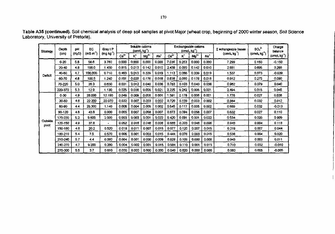
170

Table A35 (continued). Soil chemical analysis of deep soil samples at pivot Major (wheat crop, beginning of 2000 winter season, Soil ScienceLaboratory, University of Pretoria).

Strategy

Deficit

Outsidepivot

Depth(cm)

0-20

20-40

40-60

60-70

70-220

220-370

0-30

30-60

80-90

90-120

170-230

120-150

150-180

180-210

210-240

240-270

270-300

PH(HaO)

5.8

4.8

4.7

4.8

5.0

5.3

4.9

4.6

4.4

4.8

5.2

4.9

4.8

5.4

5,7

4.7

5.5

EC(mS m"1)

56.6

198.0

156.000

100.5

28.3

12.9

28.000

22.200

25.300

43.8

9.600

37.8

20.2

7.5

4.4

9.200

3.7

Bray I P(mg kg')

3.780

1.430

0.710

1.240

0.630

1.130

12.190

22.070

1.140

0.900

2.000

-

0.520

0.570

0.060

0.280

0.610

Soluble cations(cmol,; kga)

Ca1*

0.000

0.815

0.463

0.151

0.031

0.025

0.049

0.032

0.008

0.065

0.003

0.052

0.018

0.005

0.004

0.004

0.000

Kv

0.000

0.013

0.013

0.020

0.012

0.008

0.009

L0.007

0.004

0.007

0.003

0.016

0.011

0.001

0.001

0.002

0.000

Mg2*

0.000

0.142

0.339

0.176

0.040

0.005

0.006

0.003

0.005

0.058

0.001

0.048

0.007

0.003

0.000

0.001

0,000

Na*

0.000

0,010

0.019

0,018

0.036

0.021

0.001

0.002

0.002

0.007

0.022

0.006

0.015

0.015

0.009

0.015

0.000

Exchangeable cations(cmolc kg"1)

Ca1*

7.036

2.439

1.113

0.638

0.783

2.225

1.591

0.726

0.545

0.673

0.420

0.686

0.077

0.444

0.829

0.584

0.040

K*

0.263

0.090

0.066

0.080

0.103

0.242

0.178

0.133

0.117

0.094

0.091

0,203

0.120

0.076

0.105

0.110

0.020

Mg2*

0.000

0.142

0.339

0.176

0.040

0.006

0.006

0.003

0.005

0.058

0.001

0.048

0.007

0.003

0.000

0.001

0.000

Na*

0.000

0.010

0.019

0.018

0.036

LO.021

0.001

0.002

0.002

0.007

0.022

0.006

0.015

0.015

0.009

0.015

0.000

1 echangeable bases(cmoUkg1)

7.299

2.681

1.537

0.912

0.962

2.494

1.776

0.864

0.669

0.832

0.534

0.943

• 0.219

0.538

0.943

0.710

0.060

SO42"

(cmoU kg"1}

0.150

0.695

0.873

0.275

0.079

0.015

0,027

0.032

0.032

0.027

0.020

0.004

0.007

0.004

0.003

0.032

0.005

Chargebalance

(cmoUg"^)

-0.150

0.285

-0.039

0.090

0.040

0.045

0.038

0.012

-0.013

0.110

0.009

0.118

0.044

0.020

0.011

-0.010

-0.005

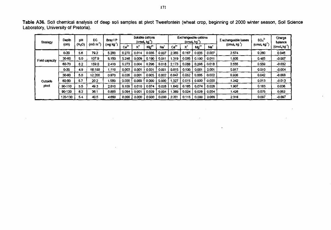
171

Table A36. Soil chemical analysis of deep soil samples at pivot Tweefontein (wheat crop, beginning of 2000 winter season, Soil ScienceLaboratory, University of Pretoria).

Strategy

Field capacity

Outsidepivot

Depth(cm)

0-30

30-60

60-70

0-30

30-60

60-90

90-110

90-120

120-130

PH(HiO)

5.6

5.0

6.2

4.9

5.0

5.7

5.5

6.2

5.4

EC(mS m'1)

79.2

107.9

159.0

16.100

12.200

20.2

49.3

36.1

40.5

Bray I P(mg kg1)

5.280

5.150

2,410

1.110

0.970

1.580

2.810

0.8O0

4.650

Soluble cations(cmolc kg"1)

Ca2t

0,270

0.248

0.273

0.003

0.026

0.000

0.109

0.094

0.000

K*

0.014

0.009

0.004

0.001

0.001

0.000

0.010

0.001

0,000

Mg*

0.035

0.190

0.296

0.001

0.005

0.000

0.074

0.029

0.000

Na*

0,007

0.011

0.018

0.001

0.002

0.000

0.026

0.004

0.000

Exchangeable cations(cmolc kg"1)

Ca2*

2.365

1.319

2.173

0.815

0.847

1.327

1.642

1.369

2.201

K*

0.167

0.085

0.068

0.100

0.052

0.015

0.165

0.024

0.115

Mg2*

0.035

0.190

0.296

0.001

0.005

0,000

0.074

0.029

0.000

Na*

0.007

0.011

0.018

0.001

0.002

0.000

0.026

0.004

0.000

I echangeable bases(cmoto kg1)

2.574

1.605

2.555

0.917

0.906

1.342

1.907

1.426

2.316

SO,2"(cmotc kg"1)

0.280

0.465

0.559

0.010

0.042

0.013

0.183

0.075

0.097

Chargebalance

(cmolokg"')

0.046

-0.007

-0.032

-0.004

-0.008

-0.013

0.036

0.053

-0.097

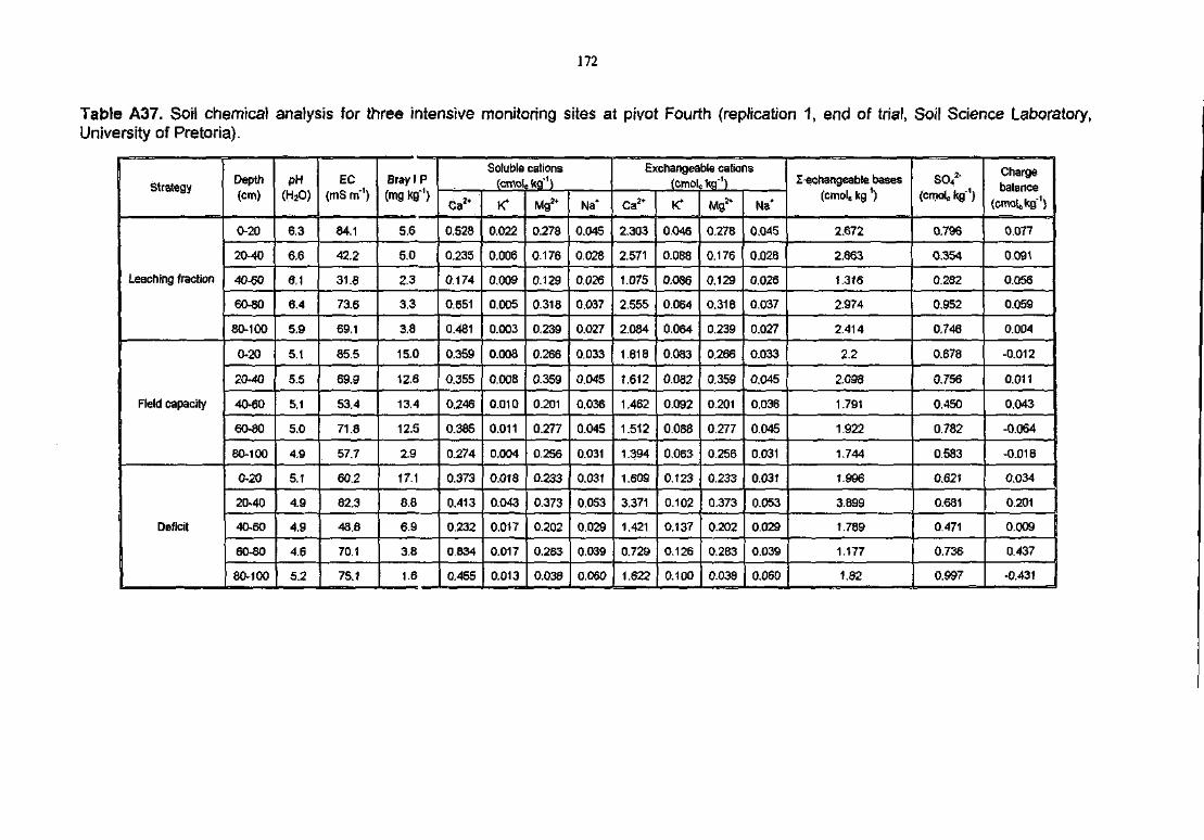
172

Table A37. Soil chemical analysis for three intensive monitoring sites at pivot Fourth (replication 1, end of trial, Soil Science Laboratory,University of Pretoria).

Strategy

Leaching fraction

Field capacity

Deficit

Depth(cm)

0-20

20-40

40-60

60-80

80-100

0-20

20-40

40-60

60-80

80-100

0-20

20-40

40-60

60*80

80-100

PH(HaO)

6.3

6.6

6.1

6.4

5.9

5.1

5.5

5.1

5.0

4.9

5.1

4.9

4.9

4.6

5.2

EC<mS m"1)

84.1

42.2

31.8

73.6

69.1

85.5

69.9

53.4

71.8

57.7

60.2

82.3

48.8

70.1

75.1

Bray I P(mgkg-1)

5.6

5.0

2.3

3.3

3.8

15.0

12.6

13.4

12.5

2.9

17.1

8.8

6.9

3.8

1.6

Soluble cations(crcroic kg'1)

Ga2'

0.528

0.235

0.174

0.651

0.481

0.359

0.355

0.246

0.385

0.274

0.373

0.413

0.232

0.834

0.455

K*

0.022

0.006

0.009

0.005

0.003

0.008

0.008

0.010

0.011

0.004

0.018

0.043

0.017

0.017

0.013

Mg2t

0.278

0.176

0.129

0.318

0.239

0.266

0.359

0.201

0.277

0.256

0.233

0.373

0.202

0.283

0.038

Na*

0.045

0.028

0.026

0.037

0.027

0.033

0.045

0.036

0.045

0.031

0.031

0.053

0.029

0.039

0.060

Exchangeable cations(cmolc kg"1)

Ca2*

2.303

2.571

1.075

2.555

2.084

1.818

1.612

1.462

1.512

1.394

1.609

3.371

1.421

0.729

1.622

K*

Q.046

0.088

0.086

0.064

0.064

0.083

0.082

0.092

0.088

0.063

0.123

O.102

0,137

0.126

0.100

Mg1*

0.278

0.176

0.129

0.318

0.239

0.266

0.359

0.201

0.277

0.256

0.233

0.373

0.202

0.283

0.038

0.045

0.028

0.026

0.037

0.027

0.033

0.045

0,036

0.045

0.031

0.031

0.053

0.029

0.039

0.060

I ^changeable bases(cmolc kg1)

2.672

2.863

1.316

2.974

2.414

2.2

2.098

1.791

1.922

1.744

1.996

3.899

1.789

1.177

1.82

SO*2"(cmolc kg"1)

0.796

0.354

0.282

0.952

0.746

0.678

0.756

0.450

0,782

0.583

0.621

0.681

0.471

0.736

0.997

Chargebalance

(Gmolj-kg"1)

0.077

0.091

0.056

0.059

0.004

-0.012

0.011

0.043

-0.064

-0.018

0.034

0.201

0.009

0.437

-0.431

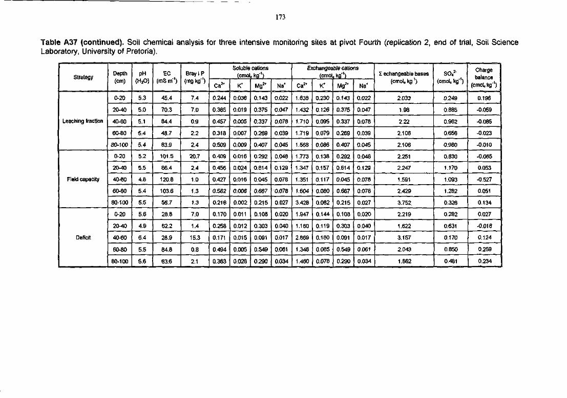
173

Table A37 (continued). Soil chemical analysis for three intensive monitoring sites at pivot Fourth (replication 2, end of trial, Soil ScienceLaboratory, University of Pretoria).

Strategy

Leaching fraction

Field capacity

Deficit

Depth(cm)

0-20

20-40

40-60

60-80

80-100

0-20

20-40

40-60

60-80

80-100

0-20

20-40

40-60

60-80

80-100

pH<H2O)

5.3

5.0

5.1

5.4

5.4

5.2

5.5

4.8

5.4

5.5

5.6

4.9

6.4

5.5

5.6

EC(mS m"1)

45.4

70.3

84.4

43.7

83.9

101.5

86.4

120.8

103.6

56.7

28.8

62.2

28.9

64.8

63.6

Bray I P(mg kg1)

7.4

7.0

0.9

2.2

2.4

20.7

2.4

1.0

1.3

1,3

7.0

1.4

15.3

0.8

2.1

Soluble cations(cmolc kg1)

Ca2*

0.244

0,385

0.457

0.318

0:509

0.409

0.456

0.427

0.582

0.216

0.170

0.258

0.171

0.494

0.363

K*

0.036

0.019

O.O05

0.007

0.009

0.016

0.024

0,016

0.006

0.002

0.011

0.012

0.015

0.005

0.028

Mg2*

0.143

0.375

0.337

0.269

0.407

0.292

0.614

0.045

0.667

0.215

0.108

0.303

0.091

0.549

0.290

Na*

0.022

0.047

0.078

0.039

0.045

0.048

0.129

0.078

0.078

0.027

0.020

0,040

0.017

0.061

0.034

Exchangeable cations<cmolckg")

Ca2*

1.638

1.432

1.710

1,719

1.568

1.773

1.347

1.351

1,604

3.428

1.947

1.160

2.869

1.348

1,460

K*

0.230

0.126

0,095

0.079

0.086

0.138

0.157

0.117

0.080

0.082

0.144

0.119

0.180

0.085

0.076

Mg2 >

0.143

0.375

0.337

0.269

0.407

0.292

0.614

0.045

0.667

0.215

0.108

0.303

0.091

0.549

0.290

Na*

0.022

0.047

0.078

0.039

0.045

0.048

0.129

0.078

0,078

0,027

0.020

0.040

0.017

0.061

0.034

I echangeable bases(cmolc kg1)

2.033

1.98

2.22

2.106

2.106

2.251

2.247

1.591

2.429

3.752,

2.219

1.622

3.157

2.043

1.862

so*3-(cmolc kg'1)

0.249

0.885

0.962

0.656

0.980

0.830

1.170

1.093

1.282

0.326

0.262

0.631

0.170

0.850

0.481

Chargebalance

(cmokkg"1)

0.196

-0.059

-0.085

-0.023

-0.010

-0.065

0.053

-0.527

0.051

0.134

0.027

-0.018

0,124

0.259

0.234

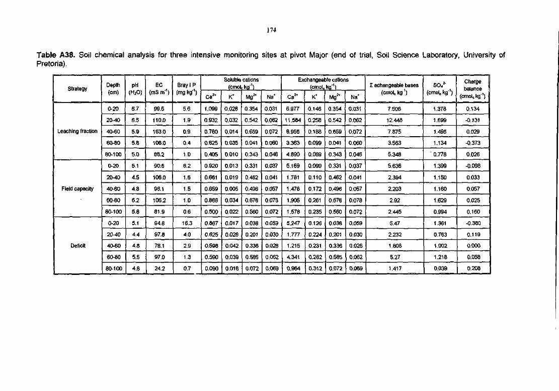
174

Table A38. Soil chemicalPretoria).

analysis for three intensive monitoring sites at pivot Major (end of trial, Soil Science Laboratory, University of

Strategy

Leaching fraction

Field capacity

Deficit

Depth(cm)

0-20

20-40

40-60

60-80

80-100

0-20

20-40

40-60

60-80

80-100

0-20

20-40

40-60

60-80

80-100

pH(HjO)

6.7

6.5

5.9

5.6

5.0

5.1

4.5

4.8

6.2

5.8

5.1

4.4

4.8

5.5

4.8

EC<mS irf1)

99.5

110.0

163.0

106.0

88.2

90.6

106.0

96.1

106.2

81.9

94.8

97.8

78.1

97.0

24.2

Bray I P(mg kg *)

5.6

1.9

0.9

0.4

1.0

6,2

1.6

1.5

1.0

0.6

16.3

4.0

2.9

1.3

0.7

Soluble cations(cmolc kg"1)

Ca3*

1.099

0.932

0.780

0.625

0.405

0.920

0.661

0.659

0.866

0.500

0.867

0.625

0.598

0.590

0.090

K*

0.028

0.032

0.014

0.035

0.010

0.013

0.019

0.005

0.034

0.022

0.017

0.026

0.042

0,039

0.016

Mg3*

0.354

0.542

0.659

0.041

0.343

0.331

0.462

0.496

0.676

0.560

0.038

0.201

0.336

Q.585

0.072

Na*

0.031

0.062

0.072

0.060

0.046

0.037

0.041

0.057

0.078

0.072

0.059

0.030

0.026

0.062

0.069

Exchangeable cations(cmoUkg1)

CaJ+

6.977

11.584

6.956

3.363

4.890

5.169

1.781

1.478

1.905

1.578

5.247

1.777

1.215

4.341

0.964

K*

0.146

0.258

0.188

0.099

0.069

0.099

0.110

0.172

0.261

0.235

0.126

0.224

0.231

0.282

0.312

Mg2*

0.354

0.542

0.659

0.041

0.343

0.331

0.462

0.496

0.676

O.560

0.038

0.201

0.336

0.585

0.072^

Na*

0.031

0.062

0.072

0.060

0.046

0.037

0.041

0.057

0.078

0.072

0.059

0.030

0.026

0.062

0.069

I ©changeable bases(cmolckg1)

7.506

12.446

7.875

3.563

5.348

5.636

2.394

2.203

2.92

2.445

5.47

2.232

1.808

5.27

1.417

SO.3"(cmolc kg"1)

1.373

1.699

1.496

1.134

' 0.776

1.399

1.150

1.160

1.629

0.994

1.361

0.763

1.0O2

1.218

0.039

Chargebalance

(cmoltkg"1)

0.134

-0.131

0.029

-0.373

0.026

-0.098

0.033

0.057

0.025

0.160

-0.3S0

0.119

0.000

0.058

0.208

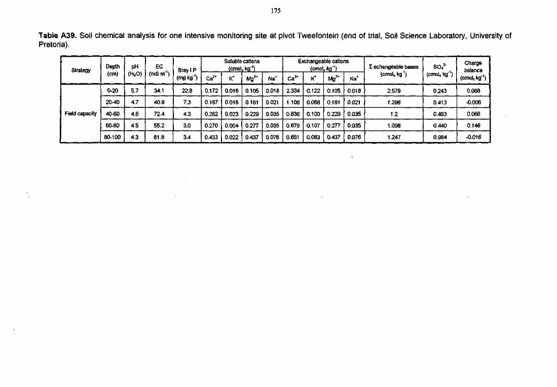
175

Table A39. Soil chemical analysis for one intensive monitoring site at pivot Tweefontein (end of trial, Soil Science Laboratory, University ofPretoria).

Strategy

Field capacity

Depth(cm)

0-20

20-40

40-60

60-80

80-100

PH(H3O)

5.7

4.7

4.6

4.5

4.3

EC(mS m"1)

34.1

40.9

72.4

55.2

81.8

Bray I P

(m kg"1)

22.8

7.3

4.3

3.0

3.4

Soluble cationsCcmo[c kg"')

Ca2'

0-172

0,187

0.262

0,270

0.433

K*

0.016

0.018

0.023

0.004

0.022

Mg3 '

0.105

0.181

0.229

0.277

0.437

Na'

0.018

0.021

0.035

0.035

0.076

Exchangeable cations(cmolo kg"1)

CaJ*

2.334

1.106

0.836

0.679

0.651

K*

0.122

0.088

0.100

0.107

0.083

MB*

0.105

0.181

0.229

0.277

0.437

Na*

0.018

0.021

0.035

0.035

0.076

X echangeable bases(enrol, kg1)

2.579

1.396

1.2

1.098

1.247

SO+3'

(cmole kg"1)

0.243

0.413

0.483

0.440

0.984

Chargebalance

(enrol, kg'1)

0.068

-0.006

0.066

0.146

-0.016

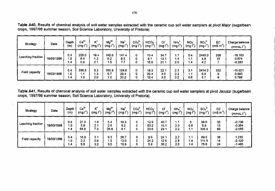
176

Table A40. Results of chemical analysis of soil water samples extracted with the ceramic cup soil water samplers at pivot Major {sugarbeancrops, 1997/98 summer season, Soil Science Laboratory, University of Pretoria).

Strategy

Leaching fraction

Field capacity

Date

18/03/1998

18/03/1998

Depthfm)

0.41.01.4

0.41.01.4

ca2+

(mg I"1)

226.06.40.9

339.51.11.0

K+

(mg f1)

19.41.32.1

3.31.32.0

Mg2+

192.66.21.5

165.80,71.0

Na+

(mg I"1)

147.48.57.7

124.620.420.2

CO32-

(mgr1)

000

000

HCO3"(mg I"1)

13.49.115.0

18.320.412.4

cr(mg r1)

34.713.121.1

22.13.03.0

NH4+

(mg I"1)

1.11.42.0

2.32.22.2

NO3"(mg I"1)

0.41.11.4

3.11.10.6

SO42"(mg I"1)

2449.04.84.2

2414.06.05.7

EC(mS m"1)

338157

33299

Charge balance

(mmolc I"1)

-18.1030.674-0.283

-15.0210.5930.768

Table A41. Results of chemical analysis of soil water samples extracted with the ceramic cup soil water samplers at pivot Jacuzzi (sugarbeancrops, 1997/98 summer season, Soil Science Laboratory, University of Pretoria).

Strategy

Leaching fraction

Field capacity

Date

18/03/1998

18/03/1998

Depth(m)

0.41.01.4

0.41.01.4

Ca2+

(mg r1)

27.05.8

64.8

16.02.25.6

K+

(mg I"1)

192.17.0

3.10.93.2

Mg2+

(mg r1)

5.42.626.8

9.21.53.5

Na+

(mg r1)

18.39.29.1

26.713.010.8

CO32"

(mg f1)

000

000

HCO3'(mg r1)

12.953.223.6

8.624.25.9

cr(mg I'1)

40.715.129.1

24.112.636.2

NH4*(mg r1)

1.12.02.2

2.22.82.0

NO3(mg r1)

00.81.1

1.11.41.4

SO*2'(mg I"1)

99.65.8

335.9

89.5111.575.6

EC(mS m"1)

351389

381424

Charge balance

(mmoicl"1)

-0.736-0.364-2.085

1.230-2.120-1.485

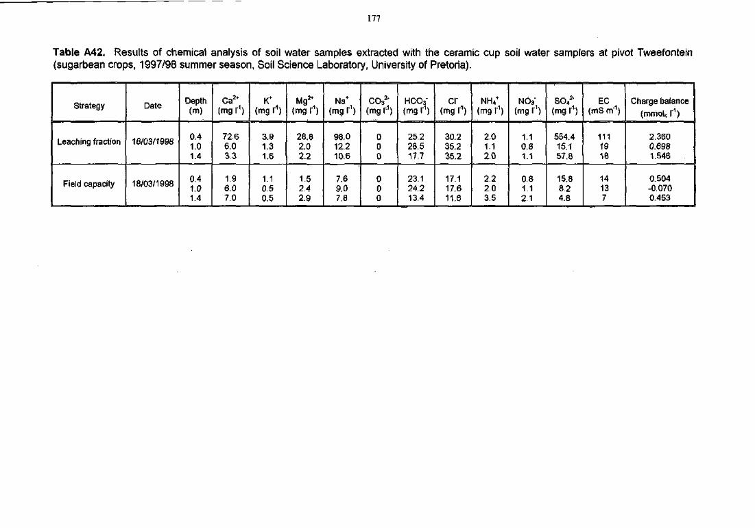
177

Table A42. Results of chemical analysis of soil water samples extracted with the ceramic cup soil water samplers at pivot Tweefontein{sugarbean crops, 1997/98 summer season, Soil Science Laboratory, University of Pretoria).

Strategy

Leaching fraction

Field capacity

Date

18/03/1998

18/03/1998

Depth(m)

0.41.01.4

0.41.01.4

Ca2t

(mg r1)

72.66.03.3

1.96.07.0

K+

(mg r1)

3.91.31.6

1.10.50.5

Mg2+

(mg r1)

28.82.02.2

1.52.42.9

Na+

(mg r1)

98.012.210.6

7.69.07.8

CO32'

(mg r1)

000

000

HCO3"(mg r1)

25.228.517.7

23.124.213.4

cr(mg r1)

30.235.235.2

17.117.611.6

NH/(mg r1)

2.01.12.0

2.22.03.5

NO3"(mg r1)

1.10.81.1

0.81.12.1

so/-(mg I"1)

554.415.157.8

15.88.24.8

EC(mS m'1)

1111918

14137

Charge balance

(mmolcr1)

2.3600.6981.546

0.504-0.0700.453

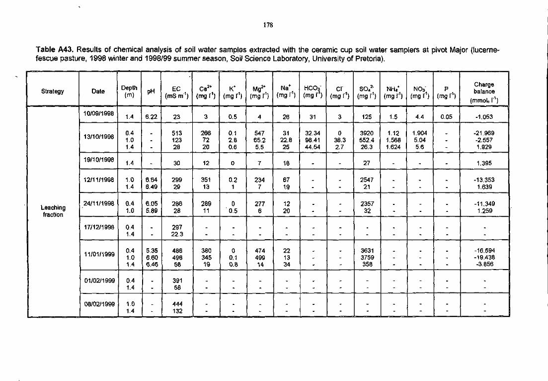
178

Table A43. Results of chemical analysis of soil water samples extracted with the ceramic cup soil water samplers at pivot Major (lucerne-fescue pasture, 1998 winter and 1998/99 summer season, Soil Science Laboratory, University of Pretoria).

Strategy

Leachingfraction

Date

10/09/1998

13/10/1998

19/10/1998

12/11/1998

24/11/1998

17/12/1998

11/01/1999

01/02/1999

08/02/1999

Depth(m)

1.4

0.41.01.4

1.4

1.01.4

0.41.0

0.41.4

0.41.01.4

0.41.4

1.01.4

pH

6.22

-

6.646.49

6.055.89

-

5.356.606.46

-

-

EC(mS m"1)

23

51312328

30

29929

28628

297223

48649858

39158

444132

Ca2*(mg r1)

3

2667220

12

35113

28911

-

38034519

-

(mg r1)

0.5

0.12.80.6

0

0.21

00.5

-

00.10.8

-

Mg2 ;(mg I'1)

4

54765.25.5

7

2347

2776

-

47449914

-

-

Na+

(mg I"1)

26

3122.825

18

6719

1220

-

221334

-

_

HCO3"(mg r1)

31

32.3496.4144.54

-

-

-

-

-

-

-

cr(mg r1)

3

038.32.7

-

-

-

-

-

-

SO,2"(mg I"1)

125

3920552.426.3

27

2547

L 21

235732

-

36313759358

-

NH4+

(mg r1)

1.5

1.121.5681.624

-

-

-

-

-

-

-

NO3"(mg r1)

4.4

1.9045.045.6

-

-

-

-

-

-

P(mg r')

0.05

-

-

-

-

-

-

-

-

Chargebalance

(mmolc I"1)

-1.053

-21.969-2.5571.929

1.395

-13.3531.639

-11.3491.259

-

-16.694-19.438-3.856

-

_

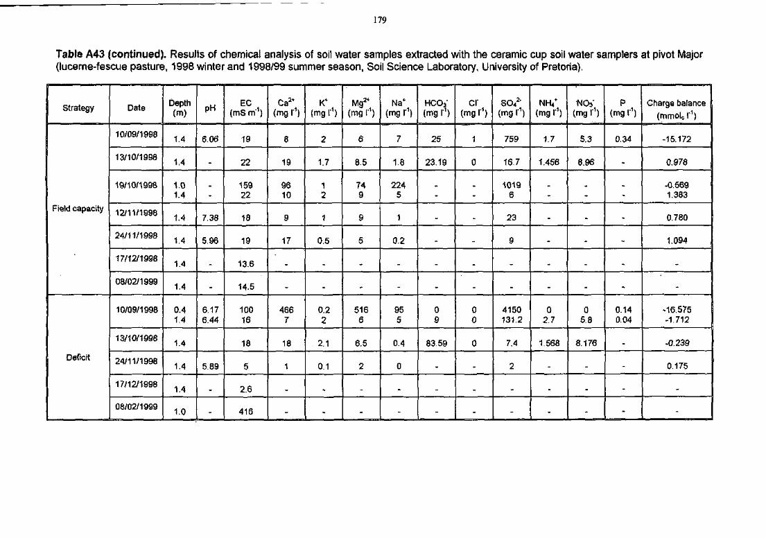
179

Table A43 (continued). Results of chemical analysis of soil water samples extracted with the ceramic cup soil water samplers at pivot Major(lucerne-fescue pasture, 1998 winter and 1998/99 summer season, Soil Science Laboratory, University of Pretoria).

Strategy

Field capacity

Deficit

Date

10/09/1998

13/10/1998

19/10/1998

12/11/1998

24/11/1998

17/12/1998

08/02/1999

10/09/1998

13/10/1998

24/11/1998

17/12/1998

08/02/1999

Depth(m)

1.4

1.4

1.01.4

1.4

1.4

1.4

1.4

0.41.4

1.4

1.4

1.4

1.0

PH

6.06

-

7.38

5.96

_

-

6.176.44

5.89

-

EC(mS m"1)

19

22

15922

18

19

13.6

14.5

10016

18

5

2.6

416

Ca2+

(mg r1)

8

19

9610

9

17

_

-

4667

18

1

-

-

K+

(mg I"1)

2

1.7

12

1

0.5

,

-

0.22

2.1

0.1

-

Mg 2 ;(mg r1)

6

8.5

749

9

5

-

5166

6.5

2

-

-

Na+

(mg r1)

7

1.8

2245

1

0.2

_

-

955

0.4

0

-

-

HCO3"(mg r1)

25

23.19

-

-

-

-

09

83.59

-

-

Cl"(mg I1)

1

0

-

-

_

-

00

0

-

-

-

SO4*(mg r1)

759

16.7

10196

23

9

-

-

4150131.2

7.4

2

-

-

NlV(mg r1)

1.7

1.456

-

-

-

-

02.7

1.568

-

-

-

NO3"(mg r1)

5.3

8.96

-

-

-

-

-

05.8

8.176

-

-

-

P(mg r1)

0.34

-

-

-

-

-

-

0.140.04

-

-

-

-

Gharge balance

(mmolc I"1)

-15.172

0.978

-0.5691.383

0.780

1.094

-

-

-16.575-1.712

-0.239

0.175

-

-

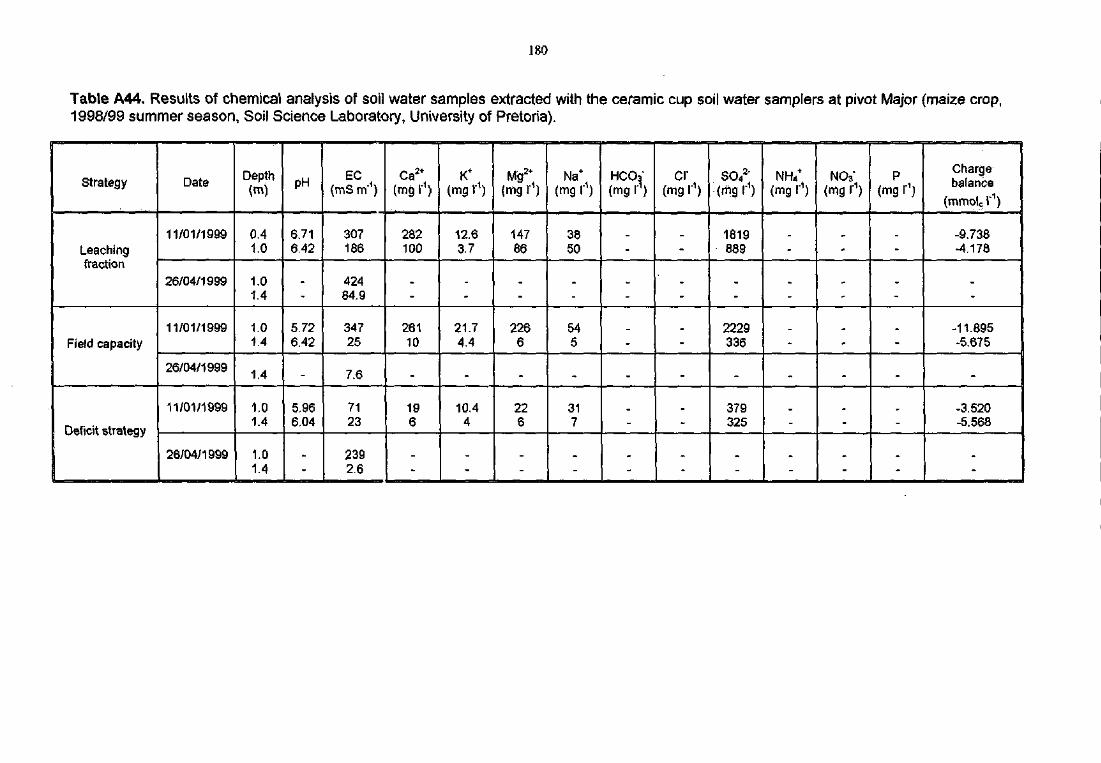
180

Table A44. Results of chemical analysis of soil water samples extracted with the ceramic cup soil water samplers at pivot Major (maize crop,1998/99 summer season, Soil Science Laboratory, University of Pretoria).

Strategy

Leachingfraction

Field capacity

Deficit strategy

Date

11/01/1999

26/04/1999

11/01/1999

26/04/1999

11/01/1999

26/04/1999

Depth(m)

0.41.0

1.01.4

1.01.4

1.4

1.01.4

1.01.4

pH

6.716,42

-

5.726.42

-

5.966.04

EC(mS rrf1)

307186

42484.9

34725

7.6

7123

2392.6

Ca2+

(mg r1)

282100

-

26110

-

196

K+

(mg r1)

12.63.7

-

21.74.4

-

10.44

Mg2+,(mg r1)

14786

-

2266

-

226

-

Na+

(mg I"1)

3850

-

545

-

317

-

HCOa'(mg I"1)

-

-

-

-

-

-

Ci-ting I"1)

;

-

-

-

-

SO42'

(mgr1)

1819889

-

2229336

-

379325

-

NrV(mg r1)

-

-

-

-

-

-

NO3"(mg r1)

;

-

-

-

-

_

P(mg r1)

;

-

-

-

-

Chargebalance

(mtmolcr1)

-9.738-4.178

-

-11.895-5.675

-

-3.520-5.568

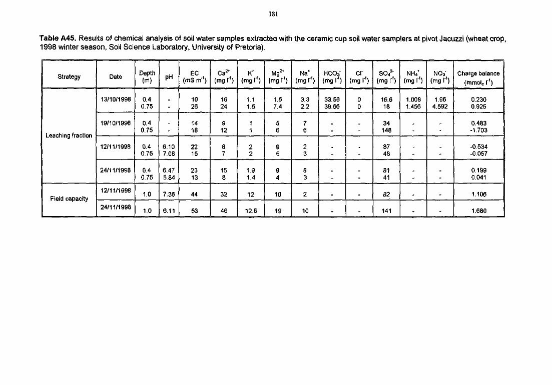
181

Table A45. Results of chemical analysis of soil water samples extracted with the ceramic cup soil water samplers at pivot Jacuzzi (wheat crop,1998 winter season, Soil Science Laboratory, University of Pretoria).

Strategy

Leaching fraction

Field capacity

Date

13/10/1998

19/10/1998

12/11/1998

24/11/1998

12/11/1998

24/11/1998

Depth(m)

0.40.75

0.40.75

0.40.75

0.40.75

1.0

1.0

pH

-

-

6.107.08

6.475.84

7.36

6.11

EC(mS rrf1)

1026

1418

2215

2313

44

53

Ca2t

(mg r1)

1624

912

87

158

32

46

K+

(mg I"1)

1.11.6

11

22

1.91.4

12

12.6

Mg2*(mg r1)

1.67.4

56

95

94

10

19

Na*(mg r1)

3.32.2

76

23

83

2

10

HCO3(mg r1)

33.5639.66

-

-

-

-

-

cr(mg I"1)

00

-

-

-

-

-

SO4Z"

(mg I"')

16.618

34148

8748

8141

8 2

141

NH4+

(mg I"1)

1.0081.456

-

-

-

-

NO3"(mg I"')

1.964.592

-

-

-

-

Charge balance

(mmolc r1)

0.2300.925

0.483-1.703

-0.534-0.057

0.1990.041

1.106

1.680

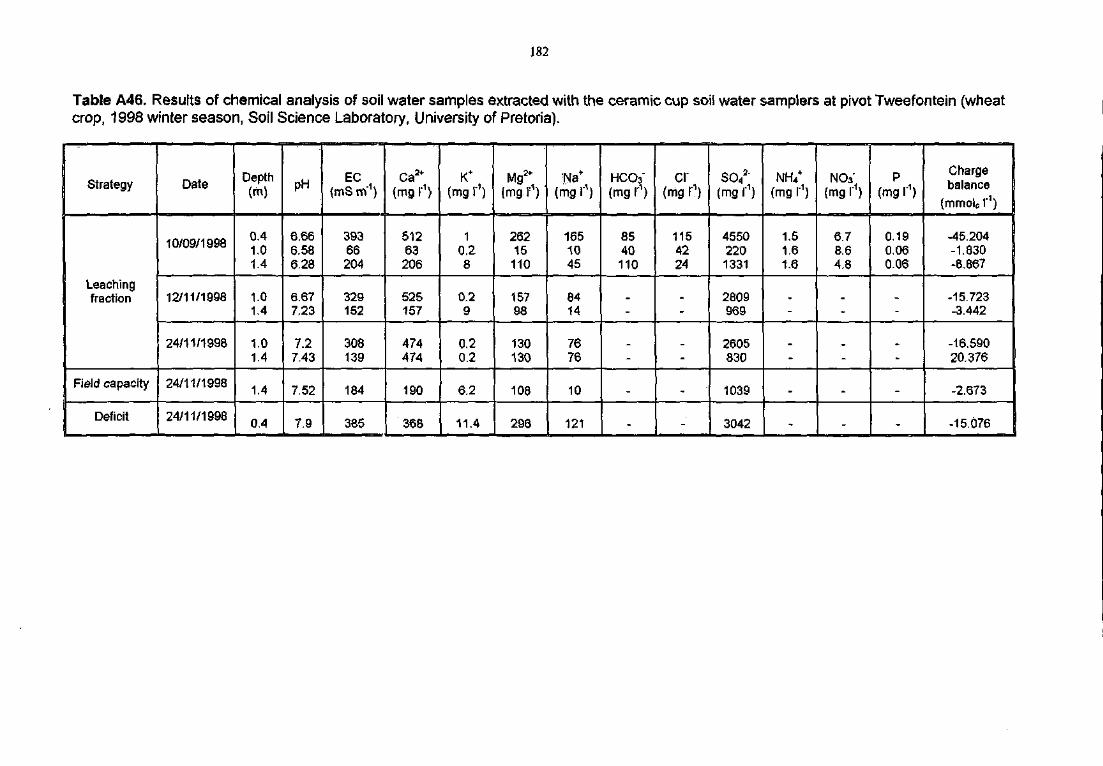
182

Table A46. Results of chemical analysis of soil water samples extracted with the ceramic cup soil water samplers at pivot Tweefontein (wheatcrop, 1998 winter season, Soil Science Laboratory, University of Pretoria).

Strategy

Leachingfraction

Field capacity

Deficit

Date

10/09/1998

12/11/1998

24/11/1998

24/11/1998

24/11/1998

Depth(m)

0.41.01.4

1.01.4

1.01.4

1.4

0.4

pH

6,666,586.28

6.677.23

7.27.43

7.52

7.9

EC(mSm1)

39366204

329152

308139

184

385

Ca2 +

(mg r1)

51263206

525157

474474

190

368

K+

(mg r1)

10.28

0.29

0.20.2

6.2

11.4

Mg2 +

(mgry

26215

110

15798

130130

108

296

:Na+

(mg r1)

1651045

8414

7676

10

121

HCO3'(mg r1)

8540110

-

-

-

-

cr(mg r1)

1154224

-

-

-

SO42'

(mg r1)

45502201331

2809969

2605830

1039

3042

NfV(mg r1)

1.51.61.6

-

-

-

-

NO3'(mg I"1)

6.78.64.8

-

-

-

-

P(mg I"1)

0.190.060.06

-

-

-

-

Chargebalance

(mmoU I'1)

-45.204-1.830-6.867

-15.723-3.442

-16.59020.376

-2.673

-15.076

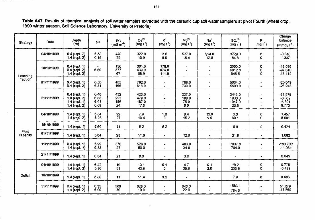
183

Table A47. Results of chemical analysis of soil water samples extracted with the ceramic cup soil water samplers at pivot Fourth (wheat crop,1999 winter season, Soil Science Laboratory, University of Pretoria).

Strategy

Leachingfraction

Fieldcapacity

Deficit

Date

04/10/1999

18/10/1999

01/11/1999

21/11/1999

04/10/1999

18/10/1999

01/11/1999

11/11/1999

21/11/1899

04/10/1999

18/10/1999

11/11/1999

Depth(m)

0.4 (repi. 2)1.4 {repl. 2)

0.4 (repl. 1)0.4 (repl. 2)1.4 (repl. 2)

0.4 (repi. 1)0.4 (repl. 2)

0.4 {repl. 1)1.0 (repl, 2)1.4 (rep!, 1)1.4 (repl. 2)

1.4 (repl. 1)1.4 (repl. 2)

1.4 (repl. 1)

1.4 (repl. 1)

0.4 (repl. 1)1.4 (repl. 1)

1.4 (repl. 1)

1.4 (repl. 1)1.4 {repl. 2)

1.4 (repl. 1}

0.4 (repl. 1)1.4 (repl. 2)

pH

6.586.15

6.80

6.506.31

6.486.356,916.09

5.545.93

5.60

5.64

5.996.38

6,54

6.425.86

6.00

6.356.09

EC(mSm"1)

44029

13037767

485466

43229315624

2227

11

28

37657

21

1951

11

50930

Ca2+

(mg I"1)

322.010.9

361.0439.068.9

782.0616.0

423.0479.0187.017.0

7.910.4

6.2

11.0

528.050.0

8.0

13.143.8

11.4

628.019.0

(mgr1)

3.60.9

178.0874.0111.0

-

-

1.30

5.2

-

-

5.10

3.2

-

Mg2 ;(mg I"1)

527.015.4

-

708.0739.0

227.0100.075.05.0

6,415.2

-

12.0

403.034.0

3.0

4.725.6

-

643.022.0

Na+

(mgr1)

214.012.0

-

-

-

13.01.9

-

-

-

-

0.12.0

-

-

SO*2"(mgr1)

3729.064.8

2000.06812.0945.5

5634.05690.0

3446.01930.01047.023.5

3.060.1

0.9

21.8

7837.0784.0

-

19.2233.8

7.9

1583.1784.0

P(mg I"1)

00

000

-

-

00

0

-

:

-

00

0

-

Chargebalance

(mmolc i1)

-8.8161.007

-19.086-97.610-13.414

-20.049-26.948

-31,978-8.062-6.3010.770

1.4570.601

0.424

1.082

-103.700-11.034

0.646

0.775-0.489

0.486

51.279-13.569

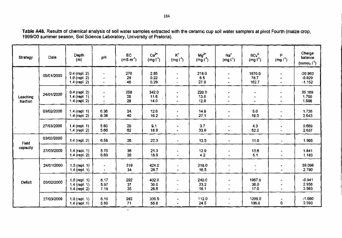
184

Table A48. Results of chemical analysis of soil water samples extracted with the ceramic cup soil water samplers at pivot Fourth (maize crop,1999/00 summer season, Soil Science Laboratory, University of Pretoria).

Strategy

Leachingfraction

Fieldcapacity

Deficit

Date

05/01/2000

24/01/2000

03/02/2000

27/03/2000

03/02/2000

27/03/2000

24/01/2000

03/02/2000

27/03/2000

Depth(m)

0.4 (repl. 2)1.0 (repl. 2)1.4 (repl. 2)

0.4 (repl. 2)1.4 (repl. 1)1.4 (repl. 2)

1.4 (repl. 1)1.4 {repl. 2)

1.4 (repl. 1)1.4 (repl. 2)

1.4 (repl. 2)

1.4 (repl. 1)1.4 (repl. 2)

1.0 {repl. 1)1.4 (rep!. 1)

1.0 {repl. 1)1.4 (repl. 1)1.4 (repl. 2)

1.0 (repl. 1)1.4 (repl. 1)

pH

-

-

6.366.38

5.805.60

6.58

5.706.60

-

6.175.977.18

6.105.80

EC(mS m"1)

2702946

2582628

2440

2962

26

3626

31934

2923735

28271

Ga i+

(mg.r1)

2.850.220.29

342.011.614.0

12.616.2

9.118.9

22.3

21.318.9

424.028.7

402.036.028.6

335.555.8

K+

(mg r1)

-

-

-

-

-

-

-

-

Mg2 ;

218.08.5

27.0

220.013.612.0

14.627.1

3.733.8

13.5

12,94.2

218.016.5

240.023.218.1

112.024.5

Na+

(mgr1)

-

-

-

-

-

-

-

-

scu2"(mg r1)

1870.078.7162.7

-

5.019.0

4.352.2

11.0

13.65.1

-

1957.036.017.0

1299.0106.0

P{mg I'1)

-

-

-

-

-

-

-

0

Chargebalance

(mrnoJc I"1)

-20.863-0.929-1.152

35.1691.7001.686

1,7262643

0.6692.637

1.995

1.8411.183

39.0962.790

-0.9412.9562.563

-10902.593

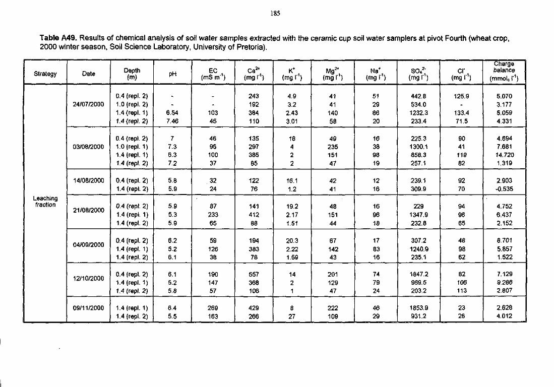
185

Table A49. Results of chemical analysis of soil water samples extracted with the ceramic cup soil water samplers at pivot Fourth (wheat crop,2000 winter season, Soil Science Laboratory, University of Pretoria).

Strategy

Leachingfraction

Date

24/07/2000

03/08/2000

14/08/2000

9i/08/?nnn

rw/fiQ/onnn

12/10/2000

09/11/2000

Depth(m)

0.4 (repl. 2)1.0 (repl. 2)1.4 (repl. 1)1.4 (repl. 2)

0.4 (repl. 2)1.0 (repl. 1)1.4 (repl. 1)1.4 (repl. 2)

0.4 (repl. 2)1.4 (repl. 2)

0.4 (repl. 2)1.4 (repl. 1)1.4 (repl. 2)

0.4 (repl. 2)1.4 (rep). 1)1.4 (repl. 2)

0.4 (repl. 2)1.4 (repl. 1)1.4 (repl. 2)

1.4 (repl. 1)1.4 (repl. 2)

pH

-

6.547.46

77.36.37.2

5.85.9

5.95.35.9

6.25.26.1

6.15.25.8

6.45.5

EC(mS m"1)

-10345

469510037

3224

8723365

5912638

19014757

269163

ca2+

(mgr1)

243192384110

13529738585

12276

14141288

19438378

557368106

429266

K+

(mg I"1)

4.93.2

2.433.01

18422

16.11.2

19.22.171.51

20.32.221.59

1421

827

Mg2 ;(mg r1)

414114058

4923515147

4241

4815144

6714243

20112947

222109

Na^(mg r1)

51298620

16389819

1216

169618

178316

747924

4629

so*2;(mg I"1)

442.8534.01232.3233.4

225.31300.1858.3257.1

239.1309.9

2291347.9232.8

307.21240.9235.1

1847.2969.5203.2

1853.9931.2

Cl"i

(mg r1)

125.9-

133.471.5

904111982

9270

949665

489862

82106113

2328

Chargebalance

(mmolcr1)

5.0703.1775.0594.331

4.6947.68114.7201.319

2.903-0.535

4.7526.4372.152

8.7015.8571.522

7.1299.2862.807

2.6284.012

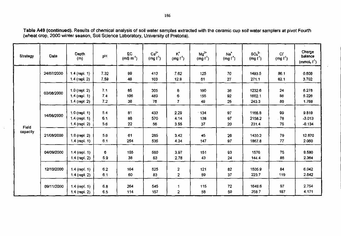
186

Table A49 (continued). Results of chemical analysis of soil water samples extracted with the ceramic cup soil water samplers at pivot Fourth(wheat crop, 2000 winter season, Soil Science Laboratory, University of Pretoria).

Strategy

Fieldcapacity

Date

24/07/2000

03/08/2000

14/08/2000

21/08/2000

04/09/2000

12/10/2000

09/11/2000

Depth(m)

1.4 {rep!. 1)

1.4 (repl. 2)

1.0(repl. 2)

1.4 (repl. 1)

1.4 (repl. 2)

1.0 (repl. 1)

1.4 (repl. 1)

1.4 (repl. 2)

1.0 (repl. 2)

1.4 (rep!. 1)

1.4 (repl. 1)

1.4 (repl. 2)

1.4 (repl. 1)

1.4 (repl. 2)

1.4 (repl. 1)

1.4 (repl. 2)

PH

7.32

7.59

7.1

7.4

7.2

5.4

6.1

5.6

5.66.1

65,9

6.26,1

6.8

6.5

EC(mSm'1}

99

48

85

106

38

81

88

22

61254

155

38

164

60

264

114

Ca2+

(mg r1)

413

103

305

483

76

433

570

56

285

535

560

63

525

83

545

157

(mg r1)

7.62

12.9

8

6

7

2.29

4.14

3.55

3.42

4.34

3.97

2.78

2

2

1

2

Mg*(mg I"1)

125

61

190

155

49

• 134

138

37

45

147

151

43

121

59

115

58

Na+

(mgr1)

70

27

36

92

25

97

97

20

26

97

93

24

8237

72

50

SO42'

(mg r1)

1493.5

271.1

1232.6

1602.1

243.3

1166.8

2158.2

231.4

1430.2

1867.8

1576

144.4

1505.9223.7

1648.6

258.7

cr<mg I1)

86.1

62.1

24

86

80

99

78

75

79

77

75

86

84

119

97

187

Chargebalance

(mmolc I"1)

0.608

3.702

6.278

5.226

1.768

9.819

-3.013

-0.134

12.870

2.060

9.580

2.364

6.042

2.642

2.754

4.171

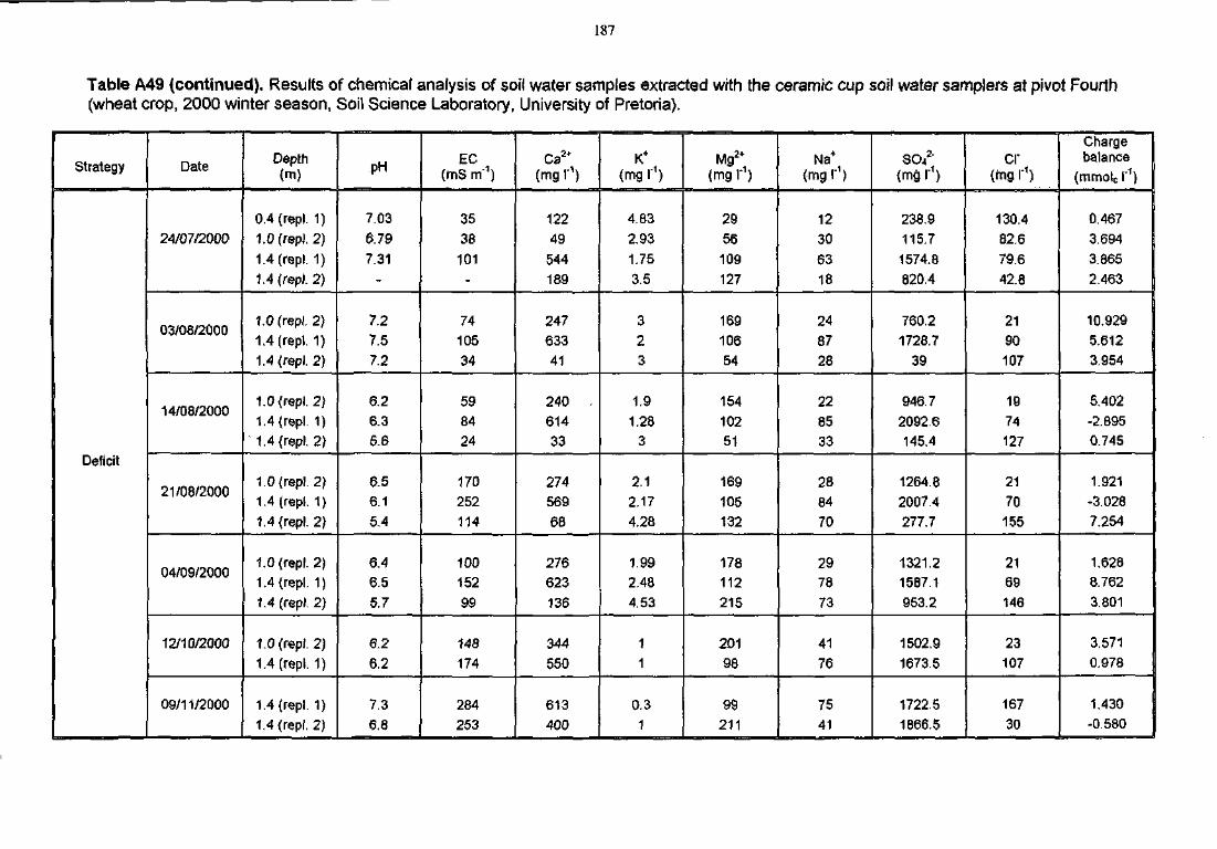
187

Table A49 (continued). Results of chemical analysis of soil water samples extracted with the ceramic cup soil water samplers at pivot Fourth(wheat crop, 2000 winter season, Soil Science Laboratory, University of Pretoria).

Strategy

Deficit

Date

24/07/2000

03/08/2000

14/08/2000

21/08/2000

04/09/2000

12/10/2000

09/11/2000

Depth(m)

0.4 (repl. 1)

1.0 (repl. 2)

1.4 (repl. 1)

1.4 (repl. 2)

1.0 (repl. 2)

1.4 (repl. 1)

1.4 (repl. 2)

1.0 {repl. 2)

1.4 (repl. 1)

1.4 (repl. 2}

1.0 (repl. 2)

1.4 (repl. 1)

1.4 (repl. 2)

1.0 (repl. 2)

1.4 (repl. 1)

1.4 (repl. 2)

1.0 (repl. 2)

1.4 (repl. 1)

1.4 (rep!. 1)

1.4 (repl. 2)

PH

7.03

6.79

7.31

7.2

7.5

7.2

6.2

6.3

5.6

6.5

6.1

5.4

6.4

6.5

5.7

6.2

6.2

7.3

6.6

EC(mSm"1)

35

38

101

74

105

34

59

84

24

170

252

114

100

152

99

148

174

284

253

Ca2+

(mg r1)

122

49

544

189

247

633

41

240 .

614

33

274

569

68

276

623

136

344

550

613

400

K*(mg I"1)

4.83

2.93

1.75

3.5

3

2

3

1.9

1.28

3

2.1

2.17

4.28

1.99

2.48

4.53

1

1

0.3

1

Mg2*(mg I"1)

29

56

109

127

169

106

54

154

102

51

169

105

132

178

112

215

201

98

99

211

Na+

(mgr1)

12

30

63

18

24

87

28

22

85

33

28

84

70

29

78

73

41

76

75

41

SO42*

(mg I"1)

238.9

115.7

1574.8

820.4

760.2

1728.7

39

946.7

2092.6

145.4

1264.8

2007.4

277.7

1321.2

1587.1

953.2

1502.9

1673.5

1722.5

1866.5

cr(mg I"1)

130.4

82.6

79.6

42.8

21

90

107

19

74

127

21

70

155

21

69

146

23

107

167

30

Chargebalance

(mmotc I"1)

0.467

3.694

3.865

2.463

10.929

5.612

3.954

5.402

-2.895

0.745

1.921

-3.028

7.254

1.628

8.762

3.801

3.571

0.978

1.430

-0.580

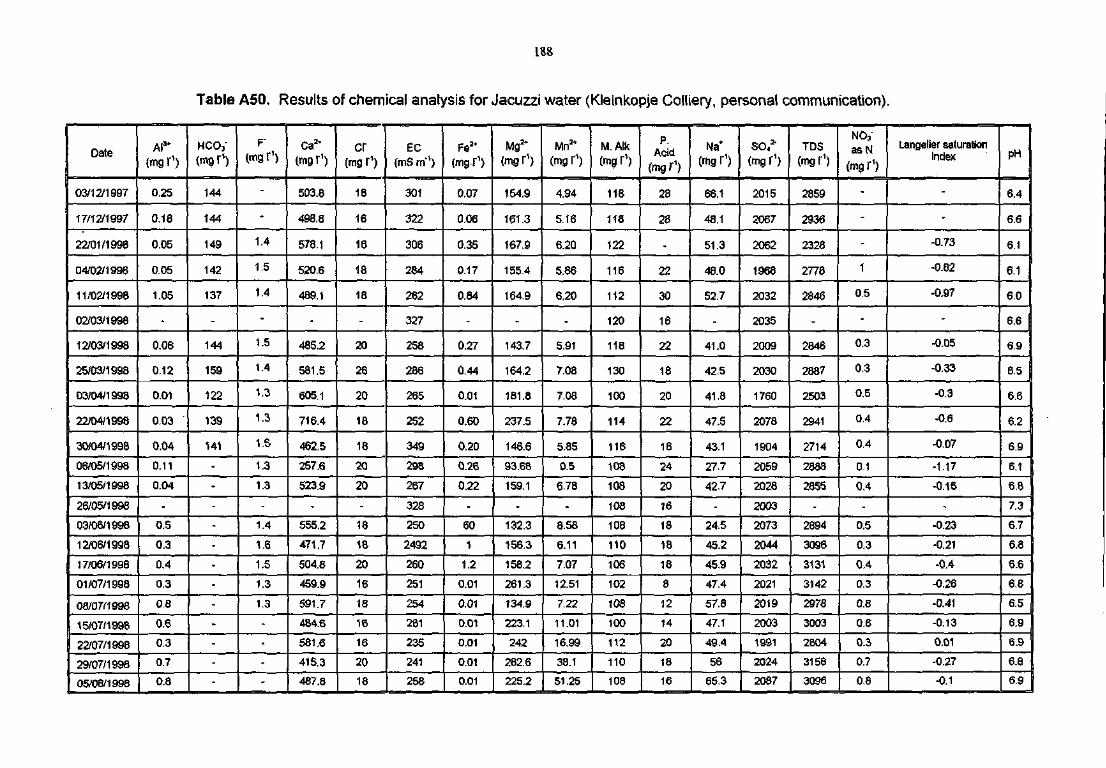
188

Table A50. Results of chemical analysis for Jacuzzi water (Kleinkopje Colliery, personal communication).

Date

03/12/1997

17/12/1997

22/01/1998

04/02/1998

11/02/1998

02/03/1998

12/03/1998

25/03/1998

03/04/1998

22/04/1998

30/04/199S

06/05/1998

13/05/1998

26/05/1998

03/06/1998

12/06/1998

17/06/1998

01/07/1998

08/07/1998

15/07/1998

22/07/1998

29/07/1998

05/08/1998

Al3*

(mg r1)

0.25

0.18

0.05

0.05

1.05

-

0.06

0.12

0.01

0.03

0.04

0.11

0.04

-

0.5

0.3

0.4

0.3

0.8

0.6

0.3

0.7

0.8

HCO3"

144

144

149

142

137

-

144

159

122

139

141

-

-

-

-

-

-

-

-

-

-

-

F"(mgr1)

-

-

1.4

1.5

1.4

-

1.5

1.4

1.3

1.3

V5

1.3

1.3

-

1.4

1.6

1.5

1.3

1.3

-

-

-

-

Ca2*(mgr1)

503.8

498.8

578.1

520.6

489.1

-

485.2

581.5

605.1

716.4

462.5

257.6

523.9

-

555.2

471.7

504.8

459.9

591.7

484.6

581.6

415.3

487.8

cr(mg r1)

18

16

16

18

18

-

20

26

20

18

18

20

20

-

18

18

20

16

18

16

16

20

18

EC(mS m")

301

322

306

284

262

327

258

286

265

252

349

298

267

328

250

2492

260

251

254

261

235

241

258

fe2 '(mgr1)

0.07

0.06

0.35

0.17

0.84

-

0.27

0.44

0.01

0.60

0.20

0.26

0.22

-

60

1

1.2

0.01

0.01

0.01

0.01

0.01

0.01

Mg2*(mg r1)

154.9

161.3

167.9

155.4

164.9

-

143,7

164.2

181.8

237.5

146.6

93.68

159.1

-

132.3

156.3

158.2

261.3

134.9

223.1

242

282,6

225.2

Mn3*

(mg i"1)

4.94

5.16

6.20

5.86

6.20

-

5.91

7.08

7.08

7.78

5.85

0.5

6.78

-

8.58

6.11

7.07

12.51

7.22

11.01

16,99

38.1

51.25

M.Alk(mg r1)

118

118

122

116

112

120

118

130

100

114

116

108

108

108

108

110

1Q6

102

108

100

112

110

108

P.Acid

(mg r1)

28

28

-

22

30

16

22

18

20

22

16

24

20

16

18

18

18

8

12

14

20

18

16

Na* ;

(mg r1)

66.1

48.1

51.3

48.0

52.7

-

41.0

42.5

41.8

47.5

43.1

27.7

42,7

-

24.5

45.2

45.9

47.4

57.8

47.1

49.4

56

65.3

SO,2"

(mg I"1)

2015

2067

2062

1968

2032

2035

2009

2030

1760

2078

1904

2059

2028

2003

2073

2044

2032

2021

2019

2003

A 991

2024

2087

TDS(mg r1)

2859

2936

2328

2778

2846

-

2846

2887

2503

2941

2714

2888

2855

-

2894

3096

3131

3142

2978

3003

2604

3158

3096

NO,"

asN

(mg r1)

-

-

-

1

0.5

-

0.3

0.3

0,5

0.4

0.4

0.1

0.4

-

0.5

0.3

0.4

0.3

0.8

0.6

0.3

0.7

0.8

Langelier saturationIndex

-

-

-0.73

-0.82

-0.97

-

-0.05

-0.33

-0.3

-0,6

-0.07

-1.17

-0.16

-

-0.23

-0.21

-0.4

-0.26

-0.41

-0.13

0.01

-0.27

-0.1

pH

6.4

6.6

6.1

6.1

6.0

6.6

6.9

6.5

6.6

6.2

6.9

6.1

6.6

7.3

6.7

6.8

Q.6

6.8

6.5

6.9

6.9

6.8

6.9

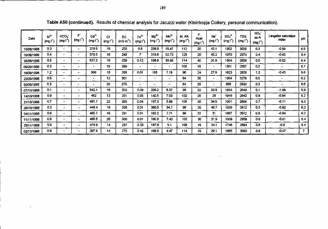
189

Table A50 (continued). Results of chemical analysis for Jacuzzi water (Kleinkopje Colliery, personal communication).

Date

15/08/1998

19/08/1998

26/08/1998

09/09/1998

16/09/1998

23/09/1998

30/09/1998

07/10/1998

14/10/1998

21/10/1998

28/10/1998

04/11/1998

11/11/1998

25/11/1998

02/12/1998

Al3t

(mgr1)

0.3

0.4

0.5

0.3

1.2

OS

0.3

0.1

0.9

0.7

0.3

0.8

0.6

0.8

0,9

HCOj"(mgr1)

-

-

-

-

-

-

-

-

-

-

-

-

-

-

-

F(mg r1)

-

-

-

-

-

-

-

-

-

-

-

-

-

-

-

Caa*(mg r1)

379,5

379.5

537,2

-

500

-

-

542,1

462

491.7

446,4

485,7

495.5

470.9

397.9

cr(mgr1)

18

16

16

18

18

12

20

16

12

22

18

18

20

14

14

EC<mS m"1)

250

249

239

269

268

301

275

302

261

265

256

291

300

237

275

Fe*(mg r1)

0.8

7

0.12

•

0.01

-

-

0.08

0.05

0.04

0.01

0.01

0.01

0.33

0.42

Mgs*(mg r1)

239.9

319.8

198.8

-

166

-

-

206.2

142.5

197.3

360.5

162.2

160.8

187.9

169.8

(mg r1)

15.47

52.73

39.88

-

7.19

-

-

8.37

7.03

5.88

34.7

7.71

H7.43

5.1

4.47

M. Afk(mgr1)

112

128

114

108

96

84

84

98

102

100

86

98

102

108

114

P.Acid

(mg r1)

20

20

40

18

24

30

20

22

26

26

26

32

30

16

18

(mgr')

43.1

45.2

31.9

-

27.6

-

-

33.8

28

34.5

46.7

31

31.9

34.1

29.1

SO,2"(mgr')

1952

1970

1904

1901

1823

1904

886

1934

1916

1901

1939

1867

1939

1746

1885

TDS(mg r1)

3029

2979

2858

2857

2838

3278

2930

2948

2942

2806

2812

2972

2959

2884

3080

NO,asN

(mgr1)

0.3

0.4

0.5

0.3

1.2

0.5

0.3

0.1

0.9

0.7

0.3

08

0.6

0.8

0.9

Langelier saturationindex

-0.59

-0.63

-0.52

-

-0.43

-

-

-1.09

-0.84

-0.71

-0.92

-0.84

-0.61

-0.6

-0.07

pH

6.5

6.4

6.4

6.7

6.6

6.2

6.6

5.9

6.2

6.3

6.2

6.2

6.4

6.4

7

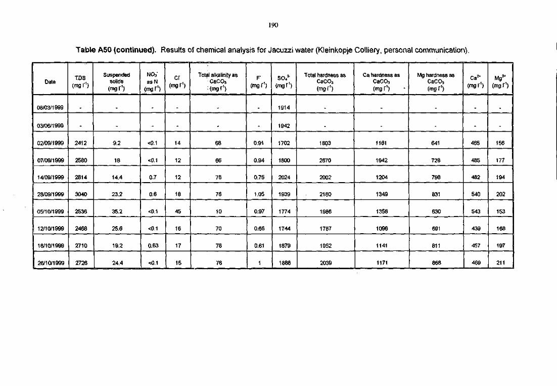
190

Table A50 (continued). Results of chemical analysis for Jacuzzi water (Kteinkopje Colliery, personal communication).

Date

08/03/1999

03/06M999

02/09/1999

07/09/1999

14/09/1999

28/09/1999

05/10/1999

12/10/1999

18/10/1999

26/10/1999

TDS

(mg r1)

•

2412

2580

2814

3040

2536

2468

2710

2726

Suspendedsolids(mg r1)

_

9.2

18

14.4

23.2

35.2

25.6

19.2

24.4

NO3"asN

(mar1)

_

<0.1

<0.1

0.7

0.6

<0.1

<0.1

0.63

<0.1

cr

-

14

12

12

18

45

16

17

15

Total alkalinity asCaCO,(mgr1)

_

68

66

76

76

10

70

78

76

F(mgr1)

0.91

0.94

0.75

1.05

0.97

0.66

0.61

1

SO42"

(mgr1)

1914

1942

1702

1800

2024

1939

1774

1744

1879

1888

Total hardness asCaCO3

(mg''1)

_

_

1803

2670

2002

2180

1986

1767

1952

2039

Ca hardness asCaCO3

(mg r1)

_

_

1161

1942

1204

1349

1356

1096

1141

1171

Mg hardness asCaCO3

(mgr1)

_

_

641

726

798

831

630

691

811

868

Ca2*

(mg r1)

_

465

485

482

540

543

439

457

469

Mg i+

(mgr')

„

156

177

194

202

153

168

197

211

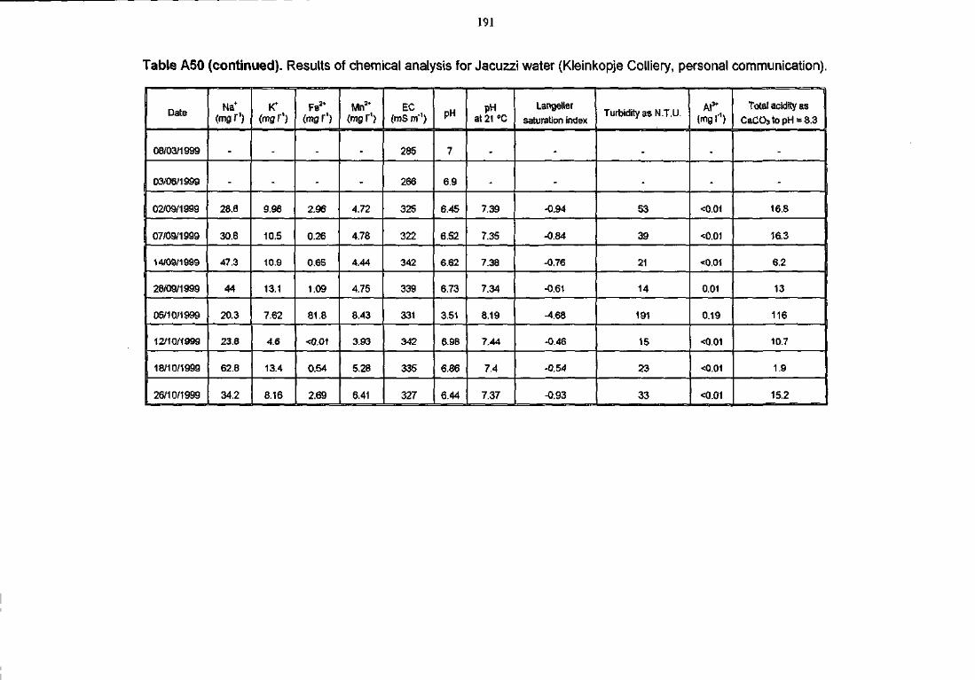
191

Table A50 (continued). Results of chemical analysis for Jacuzzi water (Kleinkopje Colliery, personal communication).

Date

08/03/1999

03/08/1999

02/09/1999

07/09/1999

14/09/1999

28/09/1999

05/10/1999

12/10/1999

18/10/1999

26/10/1999

Na*(mgl1)

28.8

30.8

47.3

44

20.3

23.8

62.8

34.2

9.98

10.5

10.9

13.1

7.62

4.6

13.4

8.16

Fe2*(mg I1)

-

2.96

0.26

0.65

1.09

81.8

<0.O1

0.54

2.69

Mn1*(mg I"1)

4.72

4.78

4.44

4.75

8.43

3.93

5.28

6.41

EC(mS m"1)

285

266

325

322

342

339

331

342

335

327

PH

7

6.9

6.45

6.52

6.62

6.73

3.51

6.98

6.86

6.44

pHat 21 "C

7.39

7.35

7.38

7.34

8.19

7.44

7.4

7.37

Langelier

saturation index

-0.94

^0.84

-0.76

-0.61

-4.68

-0.46

-0.54

-0.93

Turbidity as NT.U.

53

39

21

14

191

15

23

33

A l *{mg r1)

-

<0.01

<o.oi

<0.01

0.01

0.19

<0.01

<0.01

<0.01

Total acidify as

CaCOstopH = 8.3

-

16.8

16.3

6.2

13

116

10.7

1.9

15.2

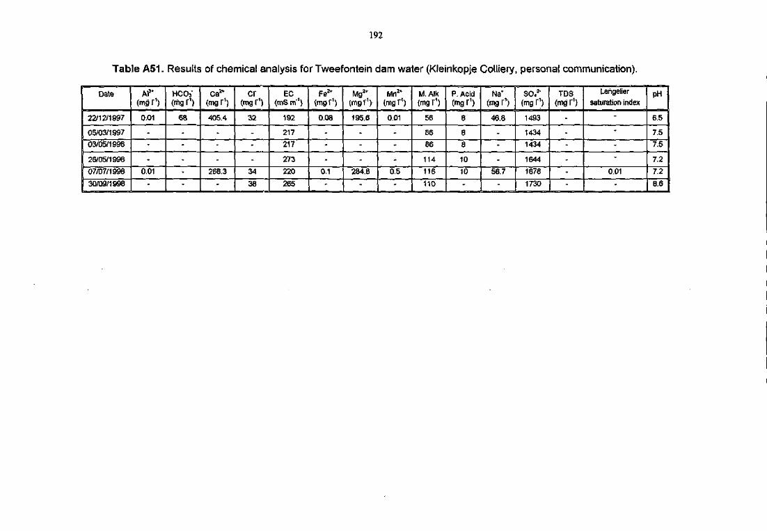
192

Table A51. Results of chemical analysis for Tweefontein dam water (Kleinkopje Colliery, personal communication).

Date

22/12/1997

05/03/1997

03/05/1998

26/05/1998

07/07/1998

30/09/1998

Al3t

(mgr1)

0.01

-

-

-

0.01

-

HCO3"(mg I"1)

68

-

-

-

-

-

Ca2v

(mg r1)

405.4

-

-

-

268.3

-

cr(mgr1)

32

-

-

-

34

38

EC(mS m"1)

192

217

217

273

220

265

(mgr1)

0.08

-

-

-

0.1

Mg3*(mgr1)

195.6

-

-

-

284.8

-

Mn2*(mgr1)

0.01

-

-

-

0.5

-

M. Alk(mgr1)

56

86

86

114

116

110

P. Acid(mg I"1)

6

e8

10

10

-

Na*(mg r1)

46.8

-

-

-

56.7

-

SO.2'(mg r1)

1493

1434

1434

1644

1678

1730

TDS(mg r1)

-

--

---

Langelier

saturation index

-

-

-

-

0.01

-

pH

6.5

7.5

7.5

7.2

7.2

8.6

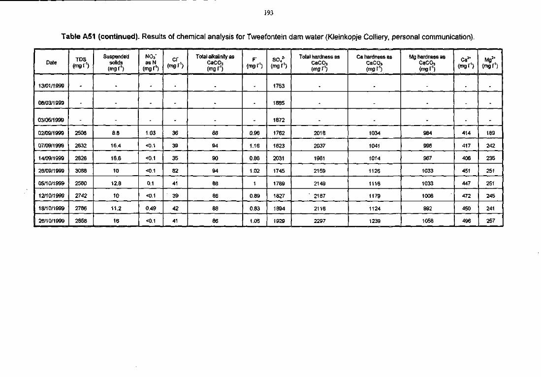
193

Table A51 (continued). Results of chemical analysis for Tweefontein dam water (Kleinkopje Colliery, personal communication).

Date

13/01/1999

08/03/1999

03/06/1999

02/09/1999

07/09/1999

14/09/1999

28/09/1999

05/10/1999

12/10/1999

18/10/1999

26/10/1999

TDS(mgr1)

-

-

2508

2632

2826

3088

2560

2742

2786

2858

Suspendedsolids

(mg r1)

-

-

8.8

16.4

18.8

10

12.8

10

11.2

16

NCVasN

(mg r1)

-

1.03

<0.1

O.1

<0.1

0.1

<0.1

0.49

<0.1

cr

-

36

39

35

82

41

39

42

41

Total alkalinity asCaCO3

(mg rf)

88

94

90

94

88

86

88

86

F(mg r1)

0.96

1.16

0.86

1.02

1

0.89

0.83

1.05

SO,*{mg r1)

1753

1885

1872

1762

1823

2031

1745

1789

1827

1894

1929

Total hardness asCaCOj{mgr1)

-

2018

2037

1981

2159

2149

2187

2116

2297

Ca hardness asCaCOj(mg I"1)

_

-

1034

1041

1014

1126

1116

1179

1124

1239

Mg hardness asCaCO3

<mg r1)

984

996

967

1033

1033

1008

992

105a

(mgr1)

_

414

417

406

451

447

472

450

496

Mg*{mg r1)

-

189

242

235

251

251

245

241

257

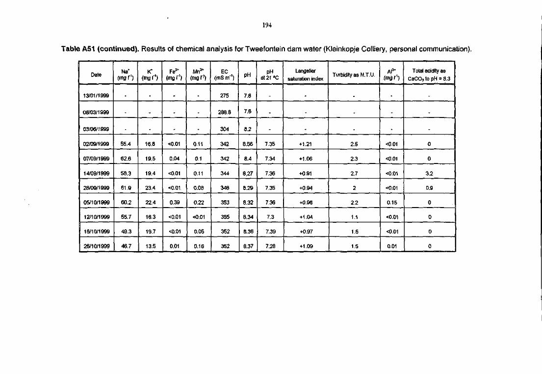
194

Table A51 (continued). Results of chemical analysis for Tweefontein dam water (Kleinkopje Colliery, personal communication).

Date

13/01/1999

08/03/1999

03/06/1999

02/09/1999

07/09/1999

14/09/1999

28/09/1999

05/10/1999

12/10/1999

18/10/1999

26/10/1999

Na*(mg r1)

5S.4

62.6

58.3

61.9

60.2

55.7

49.3

46.7

(mg r1)

-

16.3

19.5

19.4

23.4

22.4

16.3

19.7

13.5

Fe2*(mg r1)

<0.01

0.04

<0.01

<0.01,

0.39

<0.01

O.01

0.01

(mg I')

0,11

0.1

0.11

0.08

0.22

<0.01

0.05

0.16

EC(mS m"1)

275

288.8

304

342

342

344

345

353

355

352

352

pH

7.8

7.8

8.2

8.56

8.4

8,27

8.29

8.32

8.34

8.36

8.37

pHat21"C

_

7.35

7.34

7.36

7.35

7.36

7.3

7.39

7.28

Langelier

saturation index

-

+1.21

+1.06

+0.91

+0.94

+0.96

+1.04

+0.97

+1.09

Turbidity as NT,U.

_

2.5

2.3

2.7

2

2.2

1.1

1.5

1.5

Al3t

(mg r1)

<0.01

<0.01

<0.01

<0.01

0.15

<0.01

<0.01

0.01

Total acidity as

CaCOjtopH = 8.3

0

0

3.2

0.9

0

0

0

0

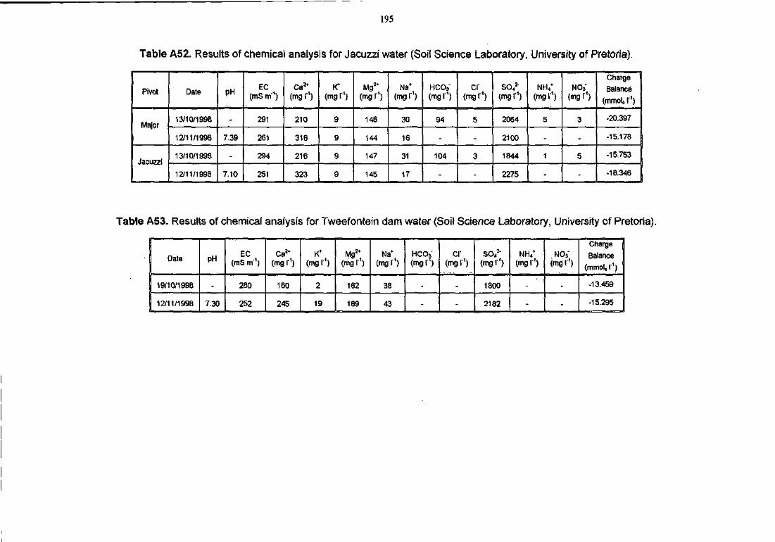
195

Table A52. Results of chemical analysis for Jacuzzi water (Soil Science Laboratory, University of Pretoria).

Pivot

Major

Jacuzzi

Date

13/10/1998

12/11/1998

13/10/1998

12/11/1998

PH

-

7.39

-

7.10

EC(mS m"1)

291

261

294

251

Caa*(mg r1)

210

316

216

323

(mg r1)

9

9

9

9

Mg2*(mgr1)

146

144

147

145

Na+

(mgr1)

30

16

31

17

HCO3"(mg r1)

94

-

104

-

cr(mg r1)

5

-

3

-

SO42"

(mgr1)

2064

2100

1844

2275

NH,*(mg r1)

5

-

1

-

NO3"(mgr1)

3

-

5

-

Charge

Balance

(mmolc r1)

-20.397

-15.178

-15.753

-18.346

Table A53. Results of chemical analysis for Tweefontein dam water (Soil Science Laboratory, University of Pretoria).

Date

19/10/1998

12/11/1998

PH

-

7.30

EC(mS tn'1)

280

252

Ca3t

(mg I'1)

180

245

K*(mg r1)

2

19

Mg5;(mg I"1)

, 162

189

Na*(mg I"1)

38

43

HCO?"( m g i )

-

-

cr(mg r1)

-

-

SO*3'(mg I'')

1800

2182

NhV(mg r1)

-

-

NO3"(mgr')

-

-

Charge

Balance

(mmo1= I"1)

-13.459

-15.295

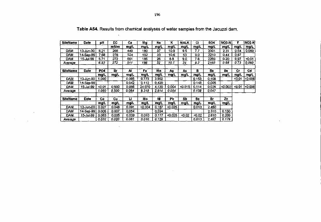
1%

Table A54. Results from chemical analyses of water samples from the Jacuzzi dam.

SlteName

DAMDAMDAM

Average

SiteName

DAMDAMDAM

Average

SiteName

DAMDAMDAM

Average

Date

13-Jun-0014-Sep-9915-Jul-99

Date

13-Jun-0014-Sep-9915-Jul-99

Date

13-Jun-0014-Sep-9915-JUI-99

pH

6.217.685.716.53

mg/L1.090

<0.011.090

Comg/L0.0270.0060.0630.032

ECmS/m266278272272

Brmg/L

0.5000.500

Cumg/L0.0480.0070.0050.020

Camg/L449524561511

AlmgIL0.0950.0420.0560.064

Limg/L0.0910.0540.0390.061

Mgmg/L180192185186

Femgll.0.7730.11224.0708.318

Momg/L

<0.004

0.0100.010

Namg/L

37332632

Mnmg/L3.9020.4204.1202.814

Nimg/L0.187Q.0240.1770.129

Kmg/L10.910.68.810.1

AgmgJL

0.0040.004

Pbmg/L

<0.025

<0.025

MALKmg/L9.5539.024

Asmg/L

<0.015

Sbmg/L

<0.02

Clmg/L7.79.07.88.2

Bmg/L0.1530.1480.1140,138

Semg/L0.013

<0.020.013

SO4mg/L2001221022692160

Bamg/L0.1080.0050.0280.047

Srmg/L2.4802.3102.6102.467

NO3-Nmg/L2.310.440.200,98

Bemg/L

<0.002

Znmg(L

0.1500.2090.179

Fmg/L0.540.670.970.73

Crmg/L<0.01

<0.01

NO2-Nmg/L0.060

<O.O10.060

Cdmg/L

<:0.006

<0.006

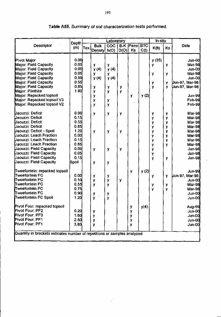
197

Table A55. Summary of soil characterization tests performed.

Descriptor

Pivot MajorMajor: Field CapacityMajor: Field CapacityMajor: Field CapacityMajor: Field CapacityMajor: Field CapacityMajor: Field CapacityMajor: PlinthiteMajor: Repacked topsoilMajor: Repacked topsoil V3Major: Repacked topsoil V2

Jacuzzi: DeficitJacuzzi: DeficitJacuzzi: DeficitJacuzzi: DeficitJacuzzi: Deficit - SpoilJacuzzi: Leach FractionJacuzzi; Leach FractionJacuzzi: Leach FractionJacuzzi: Field CapacityJacuzzi: Field CapacityJacuzzi: Field CapacityJacuzzi: Field Capacity

Tweefontein: repacked topsoilTweefontein FCTweefontein FCPweefontein FCTweefontein FCTweefontein FCTweefontein FC Spoil

Pivot Four: repacked topsoilPivot Four: PF2Pivot Four: PF3Pivot Four: PF1Pivot Four: PF1

Depth(m)

0.000.000.000.050.500.550.851.80

0.000.150.550.851.200.000.150.850.000.050.15

Spoil

0.000.100.550.750.901.20

0.201.602.503.80

laboratory

TQV;

I ex.Bulk

Density

yy(4)yy(4)

yyyyy

y

y

y

y

yyy

yy

yyyy

Quantity in brackets indicates number of repetitions

coch(O)

yy(4)yy(4)

yy

yy

y

y

y

y

yyy

yy

B-KD(O),

yy

y

y

y

y

PermKs

y

y

yyyyy

BTCC(t)

y(2)

y(2)

y(4)

or samples analyzed

ln-situ i

: K( )

y(35)y

y

yy

yyyyyyyyyyy

y

yy

r\S :

y

y

yy

yyyyyyyy

y

y

yy

: Date

Jun-00Mar-98Jun-00Mar-98Jun-00

Jun-97, Mar-98Jun-97, Mar-98

Jun-99Feb-99Feb-99

Mar-98Mar-98Mar-98Mar-98Mar-98Mar-98Mar-98Mar-98Jan-98Jan-98Jan-98

Jun-99Jun-97, Mar-98

Jun-00Mar-98Mar-98Jun-00Jun-00

Aug-99Jun-00Jun-00Jun-00Jun-00

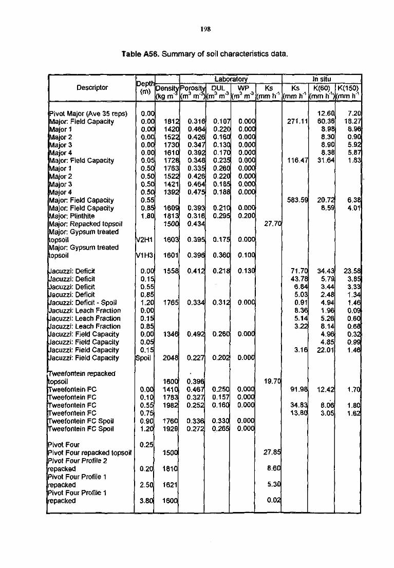
198

Table A56. Summary of soil characteristics data.

1I Descriptor

jPivot Major (Ave 35 reps)Major: Field CapacityMajor 1Major 2Major 3Major 4Major: Field CapacityMajor 1Major 2Major 3[Major 4[Major: Field CapacityMajor: Field Capacity{Major: PlirrthiteMajor: Repacked topsoilMajor: Gypsum treatedtopsoi!Major: Gypsum treatedtopsoil

Jacuzzi: DeficitJacuzzi: DeficitJacuzzi: DeficitJacuzzi: DeficitJacuzzi: Deficit - SpoilJacuzzi: Leach FractionJacuzzi: Leach FractionJacuzzi: Leach FractionJacuzzi: Field CapacityJacuzzi: Field CapacityJacuzzi: Field CapacityJacuzzi: Field Capacity

Tweefontein repackedtopsoilTweefontein FCTweefontein FCTweefontein FCTweefontein FCTweefontein FC SpoilTweefontein FC Spoil

Pivot FourPivot Four repacked topsoilPivot Four Profile 2repackedPivot Four Profile 1repackedPivot Four Profile 1repacked

Depth(m)

0.000.000.000.000.000.000.050.500.500.500.500.550.851.80

V2H1

V1H3

0.000.150.550.851.200.000.150.850.000.050.15

Spoil

0.000.100.550.750.901.20

0.25

0.20

2.50

3.80

Density(kg m"3

1812142015221730161017281763152214211392

160918131500

1603^

1601

1558

1765

134d

2048

1600141017831982

17601929

1500

1810

1621

1600

LaboratoryPorosity(m3 m"3)

0.3160.4640.4260.3470.3920.3480.3350.4260.4640.475

0.3930.3160.434

0.395

0.396

0.412

0.334

0.492

0.227

0.3960.4670.3270.252

0.3360.272

DUL(m3 m'3

0.1070.2200.1600.1300.1700.2350.2600.2200.1850.188

0.2100.295

0.175

0.360

0.218

0.312

0.26C

0.202

0.2500.1570.160

0.3300.265

WP(m3 m"3

0.0000.0000.0000.0000.0000.0000.0000.0000.0000.000

0.0000.200

0.000

0.100

0.130

o.ooo

o.ooo

o.ood

0.0000.0000.000

0.0000.000

Ks(mm h'1

27.70

19.70

27.85

8.60

5.30

0.02

In situKs

(mm h"1

271.11

116.47

583.59

71.7043.786.845.030.918.365.143.22

3.16

91.98

34.8313.80

K(60)(mm h )

12.6060.36

8.988.308.908.38

31.64

20.728.59

34.435.793.442.484.941.965.268.144.964.85

22.01

12.42

8.063.05

K(150)(mm h"1

7.2018.276.960.905.925.871.83

6.384.01

23.583.853.331.341.460.090.600.680.320.991.46

1.70

1.801.62

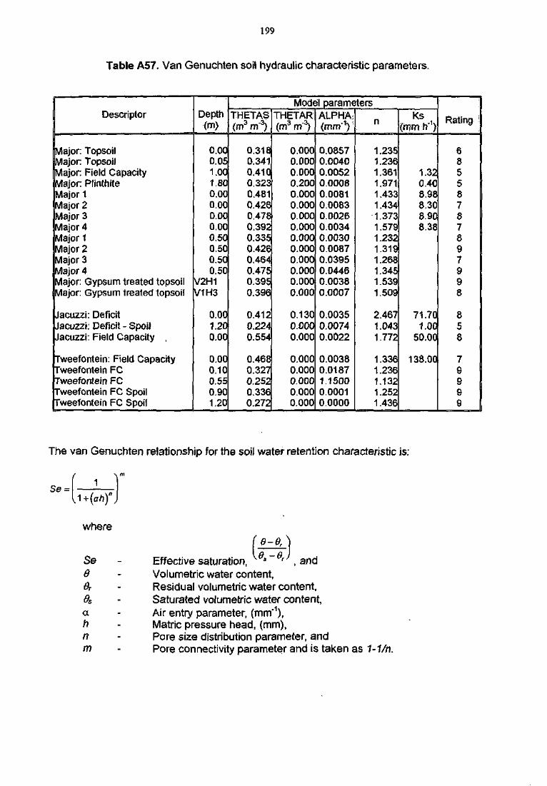
199

Table A57. Van Genuchten soil hydraulic characteristic parameters.

Descriptor

Major: TopsoilMajor: TopsoilMajor: Field CapacityMajor: PlinthiteMajor 1Major 2Major 3Major 4Major 1Major 2Major 3Major 4Major: Gypsum treated topsoilMajor: Gypsum treated topsoit

Jacuzzi: DeficitJacuzzi: Deficit - SpoilJacuzzi: Field Capacity ,

Fweefontein: Field Capacityrweefontein FCrweefontein FCTweefontein FC SpoilFweefontein FC Spoil

Depth(m)

0.000.051.001.800.000.000.000.000.500.500.500.50

V2H1V1H3

0.001.200.00

0.000.100.550.901.20

Model parametersTHETAS(m3 m"3)

0.3180.3410.4100.3230.4810.4260.4780.3920.335^0.4260.4640.4750.3950.396

0.4120.2240.554

0.4680.3270.2520.3360.272

THETAR(m3 m'3)

0.0000.0000.0000.2000.0000.0000.0000.0000.0000.0000.0000.0000.0000.000

0.1300.0000.000

0.0000.0000.0000.0000.000

ALPHA:(mrrf1)

0.08570.00400.00520.00080.00810.00830.00260.00340.00300.00870.03950.04460.00380.0007

0.00350.00740.0022

0.00380.01871.15000.00010.0000

n

1.2351.2361.3611.9711.4331.434

•1.373,1.5791.2321.3191.2681.3451.5391.509

2.4671.0431.772

1.3361.2361.1321.2521.436

Ks(mmrf1)

1.320.408.988.308.908.38

71.701.00

50.00

138.00

Rating :

68558787897998

858

79999

The van Genuchten relationship for the soil water retention characteristic is:

where

(e-Qr

Se - Effective saturation, * ~ '6 - Volumetric water content,9r - Residual volumetric water content,9s - Saturated volumetric water content,a - Air entry parameter, (mm'1),h - Matric pressure head, (mm),n - Pore size distribution parameter, andm - Pore connectivity parameter and is taken as 1-1/n.

200

The hydraulic conductivity function derived by substituting the van Genuchten retentioncharacteristic into the Mualem conductivity model is written as:

K(h) = Ks

where K(h)Ks

Unsaturated hydraulic conductivity (mm h"1) andSaturated hydraulic conductivity (mm h"1)

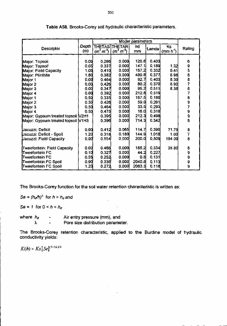
201

Table A58. Brooks-Corey soil hydraulic characteristic parameters.

Descriptor

Major: TopsoilMajor: TopsoilMajor: Field CapacityMajor: PlinthiteMajor 1Major 2Major 3Major 4Major 1Major 2Major 3Major 4Major: Gypsum treated topsoilMajor: Gypsum treated topsoil

Jacuzzi: DeficitJacuzzi: Deficit - SpoilJacuzzi: Field Capacity

Tweefontein: Field CapacityTweefontein FCFweefontein FCTweefontein FC SpoilTweefontein FC Spoil

Depth(m)

0.000.051.001.800.000.000.000.000.500.500.500.50

V2H1V1H3

0.001.200.00

0.000.100.550.901.20

THETAS(m3 m'3)

0.2660.3370.4100.3820.4640.4260.3470.3920.3350.426^0.4640.4750.3950.396

0.4120.3180.554

0.4660.3270.2520.3360.272

ModeTHETAR(m3 m'3)

0.0000.0000.0000.0000.0000.0000.0000.0000.0000.0000.0000.0000.000

. 0.000

0.0650.1800.000

0.0000.0000.0000.0000.000

I parametershd

mm

120.8147.1167.2480.8

92.780.295.2

212.8167.559.033.516.0

212.3714.3

114.7144.9200.0

185.244.2

0.82040.82083.3

Lamda

0.4030.1390.3320.3770.4030.3700.5110.5190.1800.2610.2930.3180.4980.342

0.3901.0180.509

0.3340.2270.1310.1130.118

Ks(mm h'V

1.320.418.988.308.908.38

71.701.00

184.00

35.80

Rating

69588787897998

878

89999

The Brooks-Corey function for the soil water retention characteristic is written as:

Se = ( V f r / for h > hd and

Se = 1 for 0 < h < hd

where ha Air entry pressure (mm), andPore size distribution parameter.

The Brooks-Corey retention characteristic, applied to the Burdine model of hydraulicconductivity yields:

= Ks\Sef+3JOM

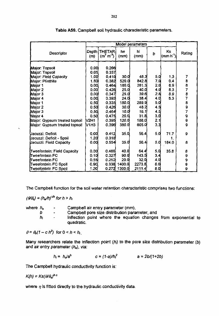
202

Table A59. Campbell soil hydraulic characteristic parameters.

Descriptor

Major: TopsoilMajor: TopsailMajor: Field CapacityMajor: PlinthiteMajor 1Major 2Major 3Major 4Major 1Major 2Major 3Major 4Major: Gypsum treated topsoilMajor: Gypsum treated topsoil

Jacuzzi: DeficitJacuzzi: Deficit - SpoilJacuzzi: Field Capacity

rweefontein: Field Capacityrweefontein FCTweefontein FCrweefontein FC Spoilrweefontein FC Spoil

Depth(m)

0.000.051.001.800.000.000.000.000.500.500.500.50

V2H1V1H3

0.001.200.00

0.000.100.550.901.20

THETAR(m3 m"3)

0.2660.3370.4100.3820.4640.4260.3470.3920.3350.4260.4640.4750.3950.396

0.4120.3180.554

0.4660.3270.2520.3360.272

Model parameters

he(mm)

30.0520.0180.025.025.024.0

180.030.010.020.0

120.0380.0

35.0

35.0

40.090.020.0

1400.01300.0

hi(mm)

48.3842.8281.3

40.039.638.4

289.948.216.131.8

188.0605.0

56.4

56.4

64,4143.532.0

2273.82111.4

b

5.07.02.04.02.84.05.04.54.53.02.13.3

5.0

5.0

5.03.44.68.0

Ks(mm h"1)

1.30.48.98.38.98.3

71.71.

184.0

35.8

Rating

788787897999

9

8

89999

The Campbell function for the soil water retention characteristic comprises two functions:

Campbell air entry parameter (mm),Campbell pore size distribution parameter, andInflection point where the equation changes from exponential toquadratic.

wherebh,

&=&s(1-ch2)

Many researchers relate the inflection point (hi) to the pore stee distribution parameter (b)and air entry parameter (he), via:

a = 2b/(1+2b)hi= hjab c

The Campbell hydraulic conductivity function is:

K(h) = K$(e/6Jbn

where 7 is fitted directly to the hydraulic conductivity data.

Appendix B

Automated tensiometers

204

Automated tensiometer nests, comprising a logger and three or four tensiometers wereinstalled at different depths, in the centre of each irrigation application rate zone on each ofthe pivots. The records were used initially to determine the direction and magnitude of thehydraulic gradients and ultimately to verify detailed modelling of the liquid fluxes.

A four-channel logger was developed to record signals from differential pressure transducersattached to tensiometers as shown in Figure B1. The automatic tensiometer housed thewater phase in a hydraulic hose, which was protected using PVC conduit. Hydraulic hosefittings sealed the water phase and provided a convenient connection to the differentialpressure transducer pressure port. The high pressure port was left open to the atmosphere.A section of clear hydraulic hose was used to connect the pressure transducer low pressureport to the main hose. This allowed for inspection of air pockets in the upper part of thetensiometer. The components were all modular, which allowed for convenient assembly inthe field to lengths determined in-situ. After careful installation, the depths D1 and D2 (FigureB1) had to be recorded for later resolution of the data. A 6V battery provided the excitationsignal to the differential pressure transducer and the response, reflecting the differencebetween the ambient air pressure and the negative water pressure in the tensiometer, wastransmitted to the logger at 12 min intervals. The logger and battery were housed in theweatherproof case on a stand above the ground.

The soil matric pressure head, hm, was taken as the difference between the ambient airpressure and the negative water pressure (or suction) at the depth D2 below the surface. Asthe ambient air pressure was taken as the reference zero pressure, the matric pressurehead was expressed as a positive quantity. The soil matric pressure head was determinedfrom the recorded differential pressure head, hdPlfrom :

hm = hdp - D1

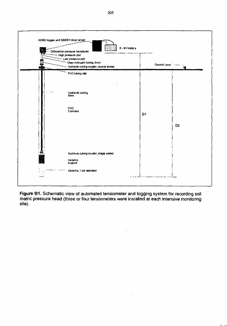
205

HOBO bQQer and SBEEH timer circuit

6 - 9V battery— Differential pressure transducer

• High pressure portLew pressure port

- Clear hydrualic tubing, 6mm

— Hydraulic tubing coupler, double endedGround Level ,

PVC tubing cap

Hydraulic tubing,6mm

PVCCconduit

D1

D2

Hydraulic tubing coupler, single ended

Ceramicsupport

Ceramic, I bar standard

Figure B1. Schematic view of automated tensiometer and logging system for recording soilmatric pressure head (three or four tensiometers were installed at each intensive monitoringsite).

Appendix C

Methods for characterization of soil material

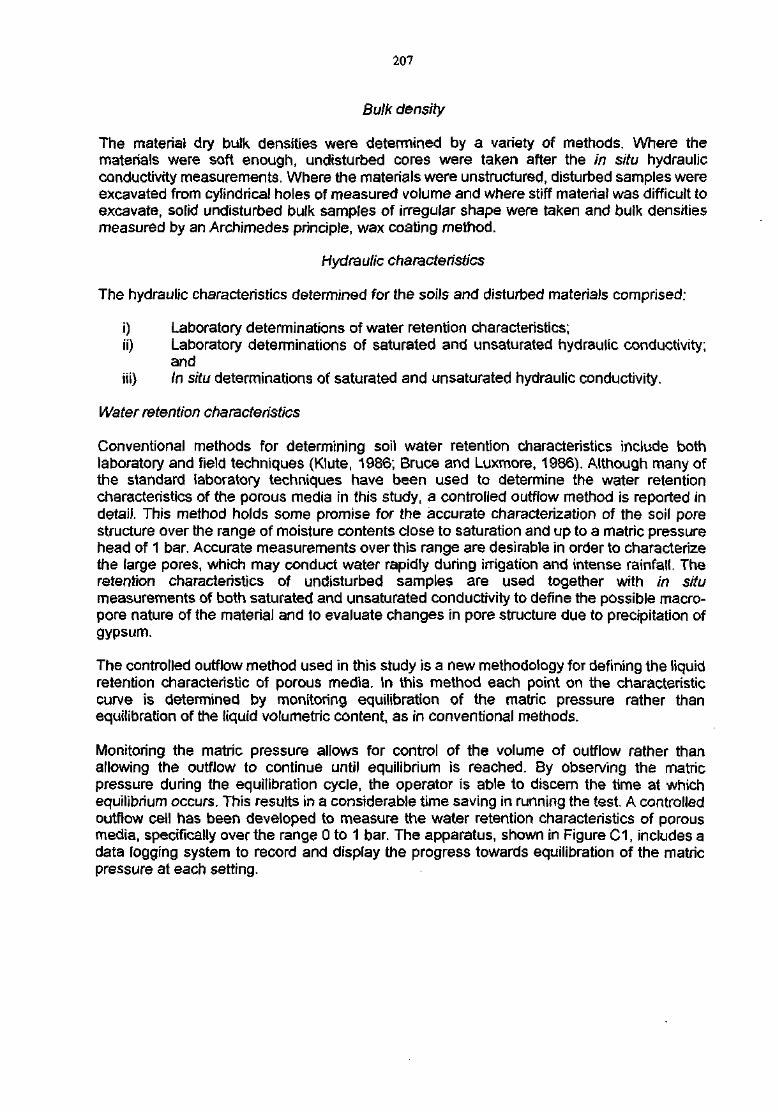
207

Bulk density

The material dry bulk densities were determined by a variety of methods. Where thematerials were soft enough, undisturbed cores were taken after the in situ hydraulicconductivity measurements. Where the materials were unstructured, disturbed samples wereexcavated from cylindrical holes of measured volume and where stiff material was difficult toexcavate, solid undisturbed bulk samples of irregular shape were taken and bulk densitiesmeasured by an Archimedes principle, wax coating method.

Hydraulic characteristics

The hydraulic characteristics determined for the soils and disturbed materials comprised:

i) Laboratory determinations of water retention characteristics;ii) Laboratory determinations of saturated and unsaturated hydraulic conductivity;

andiii) In situ determinations of saturated and unsaturated hydraulic conductivity.

Water retention characteristics

Conventional methods for determining soil water retention characteristics include bothlaboratory and field techniques (Klute, 1986; Bruce and Luxmore, 1986). Although many ofthe standard laboratory techniques have been used to determine the water retentioncharacteristics of the porous media in this study, a controlled outflow method is reported indetail. This method holds some promise for the accurate characterization of the soil porestructure over the range of moisture contents close to saturation and up to a matric pressurehead of 1 bar. Accurate measurements over this range are desirable in order to characterizethe large pores, which may conduct water rapidly during irrigation and intense rainfall. Theretention characteristics of undisturbed samples are used together with in situmeasurements of both saturated and unsaturated conductivity to define the possible macro-pore nature of the material and to evaluate changes in pore structure due to precipitation ofgypsum.

The controlled outflow method used in this study is a new methodology for defining the liquidretention characteristic of porous media. In this method each point on the characteristiccurve is determined by monitoring equilibration of the matric pressure rather thanequilibration of the liquid volumetric content, as in conventional methods.

Monitoring the matric pressure allows for control of the volume of outflow rather thanallowing the outflow to continue until equilibrium is reached. By observing the matricpressure during the equilibration cycle, the operator is able to discern the time at whichequilibrium occurs. This results in a considerable time saving in running the test. A controlledoutflow cell has been developed to measure the water retention characteristics of porousmedia, specifically over the range 0 to 1 bar. The apparatus, shown in Figure C1, includes adata logging system to record and display the progress towards equilibration of the matricpressure at each setting.

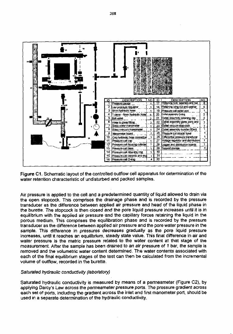
208

ID12

~~34

e" 7'

810

1 1

12-131415

| 16

DESCRIPTIONPressurejjaugeLow pressure regulator6mrn hydraulic hoseT-piece - 6mm hydraulic hoseBall valve

Hose to glass fitting.Glass water manometerGlass mercury manometerManometer boardCap hydraulic hose connecto!Pressure cell capPressure cell housing cylinderPressure cell basePressure ceil retaining ringPressure cell ceramb and ringPressure cell O-ri ng

NO,1

_JL1

_3_2211

111

11

1A

ID1 /181920212223242526272829303132

DESCRIPTIONRetaining bolt, washers and nutRetaining wing nut and washerPressure cell outlet portOutlet assembly CHing

Outlet assembly retaining capOutlet assembly glass ports andSutJet vacuum stop-cockOutlet assembly burette (50ml)Pressure transducer hoseDifferential pressure transducerVoJage regulator and distribution

Leaner and distribution boardsSupport clamps

NO.6

_6_1221

1111

14

Figure C1. Schematic layout of the controlled outflow cell apparatus for determination of thewater retention characteristic of undisturbed and packed samples.

Air pressure is applied to the cell and a predetermined quantity of liquid allowed to drain viathe open stopcock. This comprises the drainage phase and is recorded by the pressuretransducer as the difference between applied air pressure and head of the liquid phase inthe burette. The stopcock is then closed and the pore liquid pressure increases until it is inequilibrium with the applied air pressure and the capillary forces retaining the liquid in theporous medium. This comprises the equilibration phase and is recorded by the pressuretransducer as the difference between applied air pressure and the pore water pressure in thesample. This difference in pressures decreases gradually as the pore liquid pressureincreases, until it reaches an equilibrium, steady state value. This final difference in air andwater pressure is the matric pressure related to the water content at that stage of themeasurement. After the sample has been drained to an air pressure of 1 bar, the sample isremoved and the volumetric water content determined. The water contents associated witheach of the final equilibrium stages of the test can then be calculated from the incrementalvolume of outflow, recorded in the burette.

Saturated hydraulic conductivity (laboratory)

Saturated hydraulic conductivity is measured by means of a permeameter (Figure C2), byapplying Darcy's Law across the permeameter pressure ports. The pressure gradient acrosseach set of ports, including the gradient across the inlet and first manometer port, should beused in a separate determination of the hydraulic conductivity.

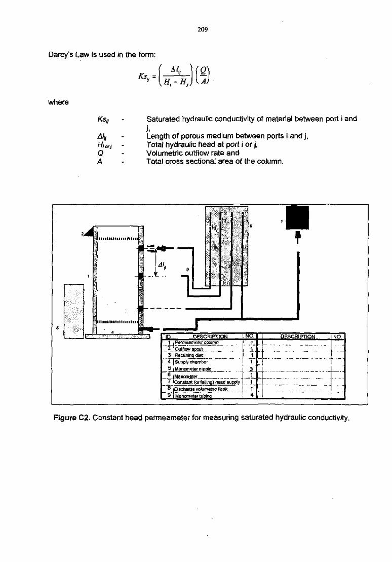
209

Darcy's Law is used in the form:

where

i or}

QA

Saturated hydraulic conductivity of material between port i andj .Length of porous medium between ports i and j ,Total hydraulic head at port i or j ,Volumetric outflow rate andTotal cross sectional area of the column.

IlirmJiiiiiiCmt

IIMdimiimiiii

ID1 ,2

""345j6_!

~78

DESCRIPTIONPermeameter columnOutflow spoutRetaining disc

Supply chamber

Manometer nipple

ManometerOonstant (or (ailing) head supply

Discharge volumetric flask

9 1 Manometer tubinq

NO.1V1131114

-

-

-

DESCRIPTION

• • • - - - — - - - -

NO.

- 1 —

Figure C2. Constant head permeameter for measuring saturated hydraulic conductivity.

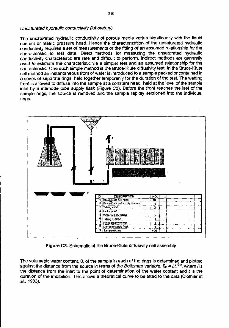
210

Unsaturated hydraulic conductivity (laboratory)

The unsaturated hydraulic conductivity of porous media varies significantly with the liquidcontent or matric pressure head. Hence the characterization of the unsaturated hydraulicconductivity requires a set of measurements or the fitting of an assumed relationship for thecharacteristic to test data. Direct methods for measuring the unsaturated hydraulicconductivity characteristic are rare and difficult to perform. Indirect methods are generallyused to estimate the characteristic via a simpler test and an assumed relationship for thecharacteristic. One such simple method is the Bruce-Klute diffusivity test. In the Bruce-Klutecell method an instantaneous front of water is introduced to a sample packed or contained ina series of separate rings, held together temporarily for the duration of the test. The wettingfront is allowed to diffuse into the sample at a constant head, held at the level of the sampleinlet by a marriotte tube supply flask (Figure C3). Before the front reaches the last of thesample rings, the source is removed and the sample rapidly sectioned into the individualrings.

ID123456*7'

' S" 9

DESCRIPTIONBruce-Klute cell ringsBruce-Klute cell supply reseivoirTubing valveCell supportWater supply tubingTubing T-pieceRapid supply funnelMarriotte supply flaskSample dishes

NO.JD

13111

£100

I1 •

Figure C3. Schematic of the Bruce-Klute diffusivity cell assembly.

The volumetric water content, 9, of the sample in each of the rings is determined and plottedagainst the distance from the source in terms of the Boltzman variable, 9B = /.f.'os, where /isthe distance from the inlet to the point of determination of the water content and t is theduration of the imbibition. This allows a theoretical curve to be fitted to the data (Clothier etal., 1983).

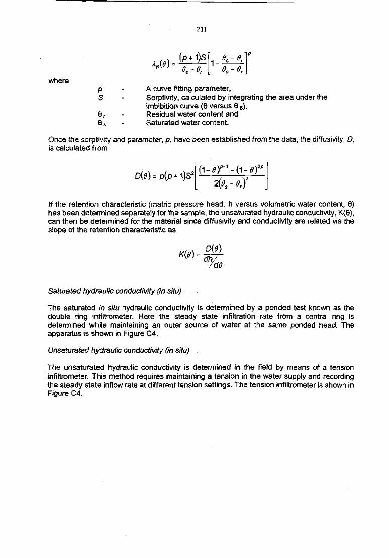
wherePS

211

XB{8) =

A curve fitting parameter,Sorptivity, calculated by integrating the area under theimbibition curve (8 versus 9 B),Residual water content andSaturated water content.

Once the sorptivity and parameter, p, have been established from the data, the diffusivity, D,is calculated from

If the retention characteristic (matric pressure head, h versus volumetric water content, 9)has been determined separately for the sample, the unsaturated hydraulic conductivity, K(9),can then be determined for the material since diffusivity and conductivity are related via theslope of the retention characteristic as

0{B)dh.yd6

Saturated hydraulic conductivity (in situ)

The saturated in situ hydraulic conductivity is determined by a ponded test known as thedouble ring infiitrometer. Here the steady state infiltration rate from a central ring isdetermined while maintaining an outer source of water at the same ponded head. Theapparatus is shown in Figure C4.

Unsaturated hydraulic conductivity (in situ) .

The unsaturated hydraulic conductivity is determined in the field by means of a tensioninfiltrometer. This method requires maintaining a tension in the water supply and recordingthe steady state inflow rate at different tension settings. The tension infiltrometer is shown inFigure C4.

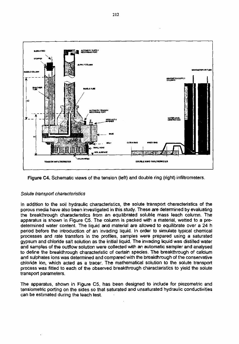
212

AUTOtMTlC SUPPLYRECOMJIN5 PORT

OUTER HNG lt*ER RMS

^'j;'-T-':'-!r^4.lrr;pv^-v u^ ;

TENSION WF11TROMETER DOUBLE RINO INFILTROMETER

Figure C4. Schematic views of the tension (left) and double ring (right) infiltrometers.

Solute transport characteristics

In addition to the soil hydraulic characteristics, the solute transport characteristics of theporous media have also been investigated in this study. These are determined by evaluatingthe breakthrough characteristics from an equilibrated soluble mass leach column. Theapparatus is shown in Figure C5. The column is packed with a material, wetted to a pre-determined water content. The liquid and material are allowed to equilibrate over a 24 hperiod before the introduction of an invading liquid. In order to simulate typical chemicalprocesses and rate transfers in the profiles, samples were prepared using a saturatedgypsum and chloride salt solution as the initial liquid. The invading liquid was distilled waterand samples of the outflow solution were collected with an automatic sampler and analysedto define the breakthrough characteristic of certain species. The breakthrough of calciumand sulphates ions was determined and compared with the breakthrough of the conservativechloride ion, which acted as a tracer. The mathematical solution to the solute transportprocess was fitted to each of the observed breakthrough characteristics to yield the solutetransport parameters.

The apparatus, shown in Figure C5, has been designed to include for piezometric andtensiometric porting on the sides so that saturated and unsaturated hydraulic conductivitiescan be estimated during the leach test.

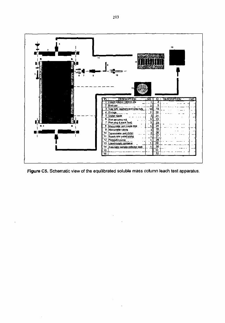
213

in123A

_5

7

~i""10"11"

'1213141516

DESCRIPTIONLeach column 100mm dig

End capCap bolt, Wayne's and wng nute

O-rings

Outlet nipple

Port S8cu.nng.nut. . . ..Port plug (Leacti Test)

Manometer port nipple (Ks)Manoriwter tubingTensiometer port (K(h))Supply and outlet tubingPeriststic pump

Liquid supply container

Automatic sample collector (opt)

NO.

2333

.-..331

111

ID3 ,3

1920

- 2 2 _2324

" 25" 26~" 27"

2829303132

DESCRIPTION I NOI

[

-

---

Figure C5. Schematic view of the equilibrated soluble mass column leach test apparatus.

Appendix D

Methods of measurement of gypsum precipitated inthe soil (Soil Science Laboratory, University of

Pretoria)

215

in this Appendix of the report, an overview of the methods to determine gypsum precipitatedin the soil is given. The following methods were considered:

• The method of Bower and Huss (1948)

A suitable amount of soil is shaken with deionised water (usually 1:5 soil to water ratio) for30 min. The sample is then centrifuged, filtrated and a 20 ml aliquot is taken from thesupernatant liquid and the EC is then determined. Soil gypsum content is then determinedby reference to a graph correlating the relationship between increase in gypsumconcentration in water up to saturation, and EC of these gypsum solutions at 25°C.

However, this method must be repeated with a wider soil to solution ratio, if the gypsumconcentration approaches the saturation level of the particular volume of water chosen. Thisprocedure must be repeated until the gypsum concentration in solution is well below thegypsum saturation level of chosen volume of water (Bower and Huss, 1948).

Drawbacks of this method

This method becomes time consuming and impractical if the gypsum concentration of alarge amount of samples must be determined. Furthermore, because of the presence (orpotential presence) of other salts, like MgSO4 and NaSO4l it is erroneous to assume that theEC of the soil solution is solely the result of gypsum in solution. This problem might influencethe accuracy of this method.

• Method of U.S. Soil Conservation Service (1972)

In this method, gypsum is extracted with successively wider soil to solution ratios, similar tothe method of Bower and Huss (1948). The difference between the method of Bower andHuss (1948) and this method is that the sulphate concentration in the solution is determined(instead of EC) of each successively wider soil to solution ratios until the sulphateconcentration in solution becomes constant which means all the gypsum is dissolved. Thesulphate concentration in solution is determined according to the conventional gravimetricBaSCv procedure described in U.S. Salinity Laboratory Staff, 1954, method 14a (U.S. SoilConservation Service, 1972; Nelson et al.( 1978).

Drawbacks of this method

Sulphates of sources other than gypsum will influence the accuracy of this method. Thebiggest drawback of this method can be the cost. To determine the gypsum concentration ofa single soil sample, two, three and most often more sulphate determinations must be made.At a cost of R15 per sulphate determination this method can become significantly moreexpensive than the previous method if the gypsum concentration of a large amount ofsamples must be determined. Furthermore, this method can be time consuming andimpractical, if the gypsum content of a large amount of samples must be determined.

• Method of Frenkel, Gerstl, Renger and van de Veen (1986)

Frenkel et al. (1986) used Na- and Cl-resin, which act as a gypsum sink by adsorbing thegypsum in solution. The resin decreases the gypsum concentration in solution, whichincreases dissolution of precipitated gypsum. The increase in NaCI concentration in solution(because of the displacement of Na+ and Cl'by Ca2+and SO4

2' respectively), also increasesthe gypsum saturation point of the water. Keren and Shainberg (1980) found that thesolubility of gypsum in a 0.1 N NaC! solution is 1.5 times higher than in deionised water. Themethod of Frenkel et al. (1986) solved the problem to find the right soil to solution ratio todissolve all the gypsum because the volume of water used in this method doesn't matter as

216

long as there is enough Na-and Cl-resins to adsorb all the gypsum and to keep the gypsumin solution low enough to cause dissolution of precipitated gypsum.

The samples with resin are shaken for 48 hours, centrifuged, filtrated and EC of thesupernatant liquid is determined. The soil gypsum content is determined by reference to agraph correlating the relationship between the difference of the EC of a sample with andwithout resin (AEC between solution with and without NaC!) and the increase in amount ofgypsum applied to a certain soil.

Drawbacks of this method

According to Frenkel et al. (1986), the correlation between AEC and amount of gypsumapplied should be constant for all soils after the interference of background electrolyte iseliminated. However, in a preliminary trial it was found (after the interference of backgroundelectrolyte is eliminated) that this relation between AEC and amount of gypsum applieddiffers from soil to soil. This difference is especially significant between clayey (in this studya 2:1 swelling clay was used) and sandy soils.

To accurately determine the gypsum content of a sample, a standard series must be madefor every single sample before the gypsum content of the sample can be determined. Thismethod can also be time consuming and impractical, if the gypsum content of a largeamount of samples must be determined. The other problem is the determination of theamount of resin that will be sufficient to extract all gypsum.

• Method of Nelson (1982)

Nelson (1982) overcame the time consuming trial and error determination to find the rightsoil to solution ratio, by using the crystal water loss method originally described by Nelson etai. (1978) to estimate the amount of gypsum in the soil and the right soil to solution ratio thatwill be sufficient to dissolve all the gypsum in the soil. The gypsum content is thendetermined by analysing sulphate concentration in solution according to the gravimetricBaSO4 procedure (U.S. Salinity Laboratory Staff, 1954). The principle of the method ofNelson et al. (1978), is that when a sample is oven dried for 24 hours at 105°C, gypsumloses its two molecules of crystal water, whereupon the crystal water stays intact if thesample is air dried for 48 hours. The mass difference between oven drying and air drying asample can thus be attributed to the loss of the crystal water of gypsum (Nelson et al.,1978). The gypsum content of the sample is then determined with the mass of the crystalwater to total mass of a gypsum molecule ratio.

Drawbacks of this method

Nelson et al. (1978) recommended this method only for taxonomic uses, while Nelson (1982)used the crystal water loss method only to determine the soil to solution ratio. This is despitethe fact that Nelson et al. (1978) found a good correlation (r2 = 0.999) between gypsumcontent determined with the crystal water loss method and gypsum content determined byanalysing sulphate concentration in solution. The biggest drawback of the crystal water lossmethod is how to correct for dehydration of the sample that is not a result of crystal waterloss of gypsum upon oven drying. Using the crystal water loss method, it takes three daysjust to estimate the amount of water necessary to dissolve all the gypsum in the sample.

• Adapted Dilution Method (ADM)

This method is a modification to the methods of Bower and Huss (1948) and the U.S. SoilConservation Service (1972). The following procedure is applied to measure precipitatedgypsum in soil samples:

217

1. 5 g to 10 g soil samples are placed in screw top bottles, and 100 cm3 of deionised wateris added.

2. The samples are shaken for 12 h to dissolve all the gypsum.3. After the 12 h shaking period, the EC of the soil solution of each sample is determined.

According to the literature, the EC of a saturated gypsum solution varies between 190mS m"1 and 235 mS m'1 (Shainberg et aJ., 1989). If the EC of the soil solutionapproaches 190 mS m'\ another 100 cm"3 is added and step (2) and (3) are repeateduntil the EC is well below 190 mS m"1. This is done to ensure that all gypsum dissolved.The EC is determined in the bottles, to make sure no solution is lost. The exact amountof water used has to be known to calculate the gypsum concentration.

4. The SCu2' concentration in solution is determined after all gypsum is dissolved.5. The SO42" concentration in saturated paste extracts with deionised water is also

determined for the same soil samples.6. The difference between the total dissolved sulphate and sulphate in the saturated paste

extract represents precipitated sulphate salts. Due to the low solubility of gypsumcompared to magnesium sulphate, this difference originates predominantly fromprecipitated gypsum.

Appendix E

Calculation of the gypsum saturation index as amethod for detecting gypsum in soils, and a

preliminary study of sulphate adsorption in soilsirrigated with saline mine water at Kleinkopje

Colliery(Dept. of Geology, University of Cape Town)

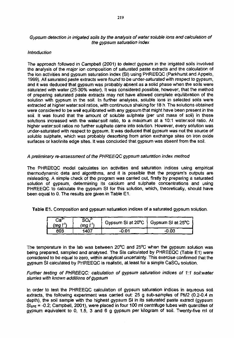
219

Gypsum detection in irrigated soils by the analysis of water soluble ions and calculation ofthe gypsum saturation index

Introduction

The approach followed in Campbell (2001) to detect gypsum in the irrigated soils involvedthe analysis of the major ion composition of saturated paste extracts and the calculation ofthe ion activities and gypsum saturation index (SI) using PHREEQC (Parkhurst and Appelo,1999). All saturated paste extracts were found to be under-saturated with respect to gypsum,and it was deduced that gypsum was probably absent as a solid phase when the soils weresaturated with water (25-30% water). It was considered possible, however, that the methodof preparing saturated paste extracts may not have allowed complete equilibration of thesolution with gypsum in the soil. In further analyses, soluble ions in selected soils wereextracted at higher watersoil ratios, with continuous shaking for 18 h. The solutions obtainedwere considered to be well equilibrated with any gypsum that might have been present in thesoil. It was found that the amount of soluble sulphate {per unit mass of soil) in thesesolutions increased with the watersoil ratio, to a maximum at a 10:1 watersoil ratio. Athigher watersoil ratios no further sulphate came into solution. However, every solution wasunder-saturated with respect to gypsum. It was deduced that gypsum was not the source ofsoluble sulphate, which was probably desorbing from anion exchange sites on iron oxidesurfaces or kaolinite edge sites. It was concluded that gypsum was absent from the soil.

A preliminary re-assessment of the PHREEQC gypsum saturation index method

The PHREEQC model calculates ion activities and saturation indices using empiricalthermodynamic data and algorithms, and it is possible that the program's outputs aremisleading. A simple check of the program was carried out, firstly by preparing a saturatedsolution of gypsum, determining its calcium and sulphate concentrations and usingPHREEQC to calculate the gypsum SI for this solution, which, theoretically, should havebeen equal to 0. The results are given in Table E1.

Table E1. Composition and gypsum saturation indices of a saturated gypsum solution.

Ca'+

(mg r1)603

SO/(mg r1)1407

Gypsum SI at 20°C

-0.01

Gypsum SI at 25°C

-0.03

The temperature in the lab was between 20°C and 25°C when the gypsum solution wasbeing prepared, sampled and analysed. The Sis calculated by PHREEQC (Table E1) wereconsidered to be equal to zero, within analytical uncertainty. This exercise confirmed that thegypsum SI calculated by PHREEQC is realistic, at least for a simple CaSO4 solution.

Further testing of PHREEQC: calculation of gypsum saturation indices of 1:1 soil:waterslum'es with known additions of gypsum

In order to test the PHREEQC calculation of gypsum saturation indices in aqueous soilextracts, the following experiment was carried out 25 g sub-samples of PM2 (0.2-0.4 mdepth), the soil sample with the highest gypsum SI in its saturated paste extract (gypsumSISPE = -0.2; Campbell, 2001), were placed in four 100 ml centrifuge tubes with quantities ofgypsum equivalent to 0, 1.5, 3 and 6 g gypsum per kilogram of soil. Twenty-five ml of

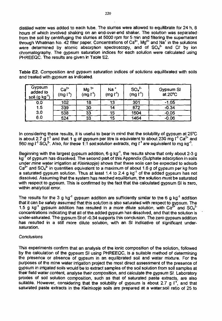
220

distilled water was added to each tube. The slurries were allowed to equilibrate for 24 h, 8hours of which involved shaking on an end-over-end shaker. The solution was separatedfrom the soil by centrifuging the slurries at 5000 rpm for 5 min and filtering the supernatantthrough Whatman No. 42 filter paper. Concentrations of Ca2+, Mg2+ and Na+ in the solutionswere determined by atomic absorption spectroscopy, and of SO4

2' and CI" by ionchromatography. The gypsum saturation indices for each solution were calculated usingPHREEQC. The results are given in Table E2.

Table E2. Composition and gypsum saturation indices of solutions equilibrated with soilsand treated with gypsum as indicated.

Gypsumadded to

soil (g kg'1)0.01.53.06.0

Ca2+

(mg I"1)

102339538524

Mg2+

(mgr1)

18303333

Na +

(mgr1)

13141515

SO42'

<mg I'1)

30187215041464

Gypsum SIat 20°C

-1.05-0.34-0.05-0.06

In considering these results, it is useful to bear in mind that the solubility of gypsum at 25°Cis about 2.7 g I"1 and that 1 g of gypsum per litre is equivalent to about 230 mg I'1 Ca2+ and560 mg I"1 SO42". Also, for these 1:1 soil.solution extracts, mg I"1 are equivalent to mg kg"1.

Beginning with the largest gypsum addition, 6 g kg'1, the results show that only about 2-3 gkg of gypsum has dissolved. The second part of this Appendix (Sulphate adsorption in soilsunder mine water irrigation at Kleinkopje) shows that these soils can be expected to adsorbCa2+ and SO4

2" in quantities equivalent to a maximum of about 1.6 g of gypsum per kg froma saturated gypsum solution. Thus at least 1.4 to 2.4 g kg"1 of the added gypsum has notdissolved. Assuming that the system has reached equilibrium, the solution must be saturatedwith respect to gypsum. This is confirmed by the fact that the calculated gypsum SI is zero,within analytical error.

The results for the 3 g kg"1 gypsum addition are sufficiently similar to the 6 g kg'1 additionthat it can be safely assumed that this solution is also saturated with respect to gypsum. The1.5 g kg"1 gypsum addition has resulted in a more dilute solution, with Ca and SO42'concentrations indicating that all of the added gypsum has dissolved, and that the solution isunder-saturated. The gypsum SI of-0.34 supports this conclusion. The zero gypsum additionhas resulted in a still more dilute solution, with an SI indicative of significant under-saturation.

Conclusions

This experiments confirm that an analysis of the ionic composition of the solution, followedby the calculation of the gypsum SI using PHREEQC, is a suitable method of determiningthe presence or absence of gypsum in an equilibrated soil and water mixture. For thepurposes of the mine water irrigation project the most direct assessment of the presence ofgypsum in irrigated soils would be to extract samples of the soil solution from soil samples attheir field water content, analyse their composition, and calculate the gypsum SI. Laboratoryproxies of soil solution composition, such as that of saturated paste extracts, are alsosuitable. However, considering that the solubility of gypsum is about 2.7 g I"1, and thatsaturated paste extracts in the Kleinkopje soils are prepared at a watersoil ratio of 25 to

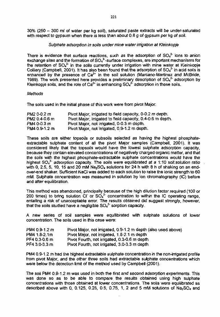
221

30% (250 - 300 ml of water per kg soil), saturated paste extracts will be under-saturatedwith respect to gypsum when there is less than about 0.8 g of gypsum per kg of soil.

Sulphate adsorption in soils undermine water irrigation at Kleinkopje

There is evidence that surface reactions, such as the adsorption of SO42~ ions to anion

exchange sites and the formation of SO42~-surface complexes, are important mechanisms for

the retention of SO42" in the soils currently under irrigation with mine water at Kleinkopje

Colliery (Campbell, 2001). It has also been found that the adsorption of SO42~ in acid soils is

enhanced by the presence of Ca2+ in the soil solution (Marcano-Marttnez and McBride,1989). The work presented here provides a preliminary description of SO4

2' adsorption byKleinkopje soils, and the role of Ca2+ in enhancing SO4

2" adsorption in these soils.

Methods

The soils used in the initial phase of this work were from pivot Major:

PM2 0-0.2 m Pivot Major, irrigated to field capacity, 0-0.2 m depth.PM2 0.4-0.6 m Pivot Major, irrigated to field capacity, 0.4-0.6 m depth.PM4 0-0.3 m Pivot Major, not irrigated, 0-0.3 m depth.PM4 0.9-1.2 m Pivot Major, not irrigated, 0.9-1.2 m depth.

These soils are either topsoils or subsoils selected as having the highest phosphate-extractable sulphate content of all the pivot Major samples (Campbell, 2001). it wasconsidered likely that the topsoils would have the lowest sulphate adsorption capacity,because they contain elevated concentrations of negatively charged organic matter, and thatthe soils with the highest phosphate-extractable sulphate concentrations would have thehighest SO4

2" adsorption capacity. The soils were equilibrated at a 1:10 soil:so|ution ratiowith 0, 2.5, 5, 10, 15 and 20 mM Na2SO4 solutions for 24 h with 8 h of shaking on an end-over-end shaker. Sufficient NaCi was added to each solution to raise the ionic strength to 60mM. Sulphate concentration was measured in solution by ion chromatography (IC) beforeand after equilibration.

This method was abandoned, principally because of the high dilution factor required (100 or200 times) to bring solution CI" or SO4

2" concentration to within the IC operating range,entailing a risk of unacceptable error. The results obtained did suggest strongly, however,that the soils studied have a negligible SO4

2' sorption capacity.

A new series of soil samples were equilibrated with sulphate solutions of lowerconcentration. The soils used in this case were:

PM4 0.9-1.2 m Pivot Major, not irrigated, 0.9-1.2 m depth (also used above)PM4 1.8-2.1 m Pivot Major, not irrigated, 1.8-2.1 m depthPF4 0.3-0.6 m Pivot Fourth, not irrigated, 0.3-0.6 m depthPF4 3.0-3.3 m Pivot Fourth, not irrigated, 3.0-3.3 m depth

PM4 0.9-1.2 m had the highest extractable sulphate concentration in the non-irrigated profilefrom pivot Major, and the other three soils had extractable sulphate concentrations whichwere below the detection limit of the method used by Campbell (2001).

The soil PM4 0.9-1.2 m was used in both the first and second adsorption experiments. Thiswas done so as to be able to compare the results obtained using high sulphateconcentrations with those obtained at lower concentrations. The soils were equilibrated asdescribed above with 0, 0.125, 0.25, 0.5, 0.75, 1, 2 and 5 mM solutions of Na2SO4 and

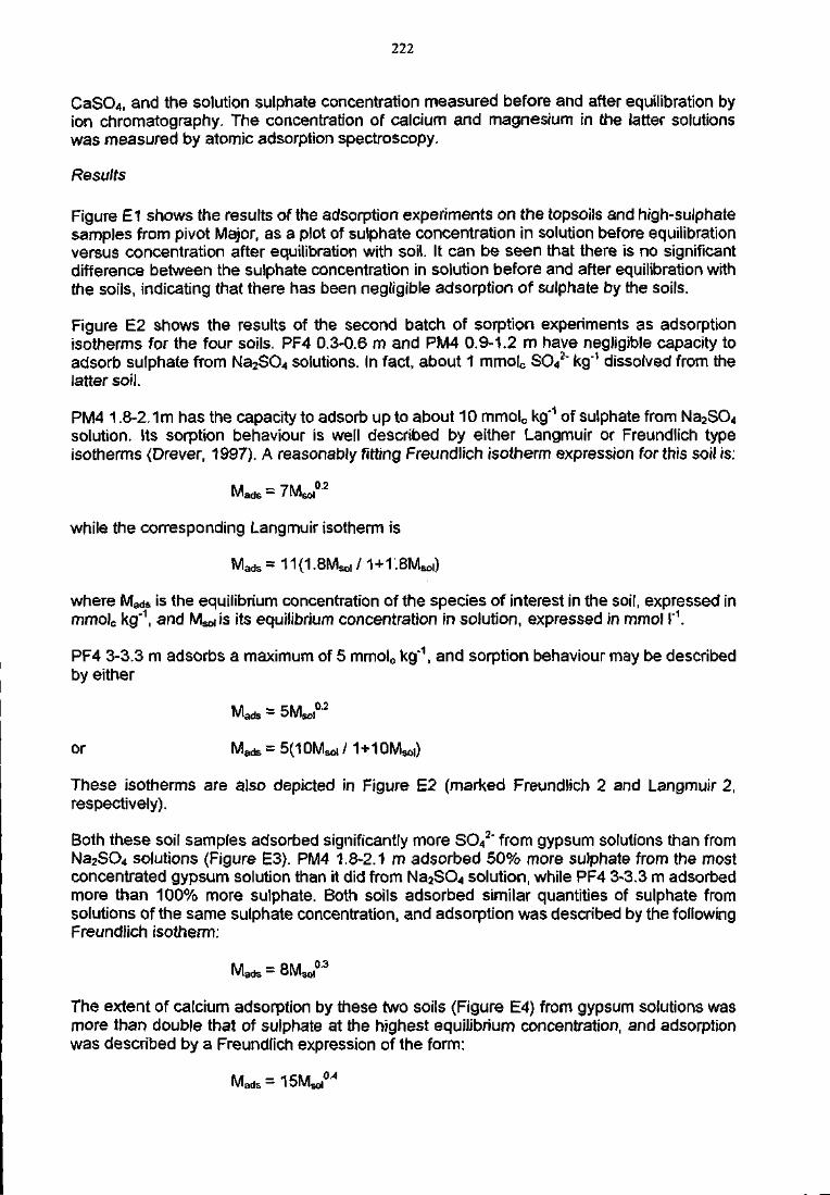
222

CaSO4, and the solution sulphate concentration measured before and after equilibration byion chromatography. The concentration of calcium and magnesium in the latter solutionswas measured by atomic adsorption spectroscopy.

Results

Figure E1 shows the results of the adsorption experiments on the topsoils and high-sulphatesamples from pivot Major, as a plot of sulphate concentration in solution before equilibrationversus concentration after equilibration with soil. It can be seen that there is no significantdifference between the sulphate concentration in solution before and after equilibration withthe soils, indicating that there has been negligible adsorption of sulphate by the soils.

Figure E2 shows the results of the second batch of sorption experiments as adsorptionisotherms for the four soils. PF4 0.3-0.6 m and PM4 0.9-1.2 m have negligible capacity toadsorb sulphate from Na2SO4 solutions. In fact, about 1 mmolc SO4

2" kg'1 dissolved from thelatter soil.

PM4 1.8-2.1m has the capacity to adsorb up to about 10 mmolc kg'1 of sulphate from Na2SO4

solution. Its sorption behaviour is well described by either Langmuir or Freundlich typeisotherms (Drever, 1997). A reasonably fitting Freundlich isotherm expression for this soil is:

Mads=7Mso,0-2

while the corresponding Langmuir isotherm is

Mads =11(1.8Mao l /1+1-.

where Mads is the equilibrium concentration of the species of interest in the soil, expressed inkg'1, and Msoris its equilibrium concentration in solution, expressed in mmo! I"1.

PF4 3-3.3 m adsorbs a maximum of 5 mmolc kg"1, and sorption behaviour may be describedby either

Mads = U,

or Mads = 5 ( 1 0 M « I / 1 + 1 0 M « I )

These isotherms are also depicted in Figure E2 (marked Freundlich 2 and Langmuir 2,respectively).

Both these soil samples adsorbed significantly more SCV' from gypsum solutions than fromNa2SC>4 solutions (Figure E3). PM4 1.8-2.1 m adsorbed 50% more sulphate from the mostconcentrated gypsum solution than it did from Na2SO4 solution, while PF4 3-3.3 m adsorbedmore than 100% more sulphate. Both soils adsorbed similar quantities of sulphate fromsolutions of the same sulphate concentration, and adsorption was described by the followingFreundlich isotherm:

The extent of calcium adsorption by these two soils (Figure E4) from gypsum solutions wasmore than double that of sulphate at the highest equilibrium concentration, and adsorptionwas described by a Freundlich expression of the form:

Mads = 1 5 M J0.4

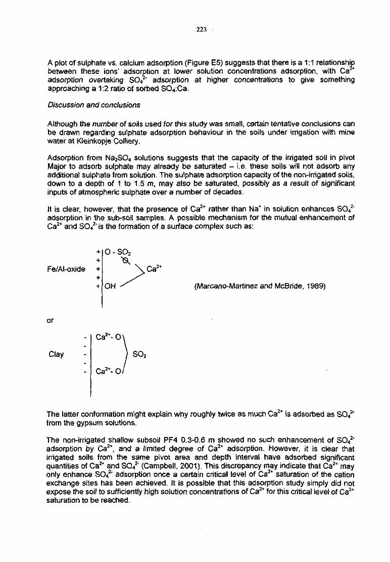
223

A plot of sulphate vs. calcium adsorption (Figure E5) suggests that there is a 1:1 relationshipbetween these ions' adsorption at lower solution concentrations adsorption, with Ca2+

adsorption overtaking SO42' adsorption at higher concentrations to give something

approaching a 1:2 ratio of sorbed SO4.Ca.

Discussion and conclusions

Although the number of soils used for this study was small, certain tentative conclusions canbe drawn regarding sulphate adsorption behaviour in the soils under irrigation with minewater at Kleinkopje Colliery.

Adsorption from Na2SC>4 solutions suggests that the capacity of the irrigated soil in pivotMajor to adsorb sulphate may already be saturated - i.e. these soils will not adsorb anyadditional sulphate from solution. The sulphate adsorption capacity of the non-irrigated soils,down to a depth of 1 to 1.5 m, may also be saturated, possibly as a result of significantinputs of atmospheric sulphate over a number of decades.

It is clear, however, that the presence of Ca2+ rather than Na+ in solution enhances SO42"

adsorption in the sub-soii samples. A possible mechanism for the mutual enhancement ofCa2+ and SO4

2~is the formation of a surface complex such as:

++

Fe/AI-oxide +++

or

Clay

o-so2

OH

Ca2+

(Marcano-Martinez and McBride, 1989)

Ca2+-O<

Ca2+-OJ

SO,

The latter conformation might explain why roughly twice as much Ca2+ is adsorbed as SO42"

from the gypsum solutions.

The non-irrigated shallow subsoil PF4 0.3-0.6 m showed no such enhancement of SO42'

adsorption by Ca2+, and a limited degree of Ca2+ adsorption. However, it is clear thatirrigated soils from the same pivot area and depth interval have adsorbed significantquantities of Ca2+ and SO4

2" (Campbell, 2001). This discrepancy may indicate that Ca2+ mayonly enhance SO4

2' adsorption once a certain critical level of Ca2+ saturation of the cationexchange sites has been achieved. It is possible that this adsorption study simply did notexpose the soil to sufficiently high solution concentrations of Ca2+ for this critical level of Ca2+

saturation to be reached.

224

Finally, turning to the relationship between sulphate adsorption and gypsum precipitation,the capacity of the soils PM4 1.8-2.1 m and PF4 3.0-3.3 m to adsorb sulphate from the soilsolution can described by the Freundlich isotherm:

0.3Mads = 8M?0|'

If MSO| is set to 15.6 mmol I'1, the concentration of sulphate in a saturated solution of gypsum,then Mads has a value of 18.2 mmolc kg"1. This is an estimate of the concentration ofadsorbed sulphate in these soils at equilibrium with a saturated solution of gypsum. Putanother way, and assuming that SO4

2" is bound in surface complexes with equivalentquantities of Ca2+, the adsorption of Ca2+ and SO4

2" is equivalent to 9.1 mmol of gypsum, i.e.1.6 g gypsum per kg of soil.

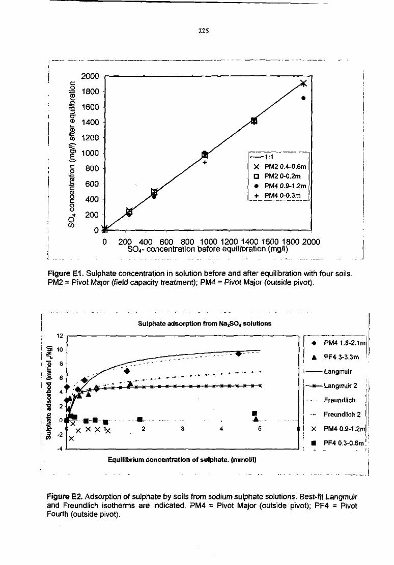
225

1:1PM2 0.4-0.6mPM2 0-0.2mPM4 0.9-1.2mPM4 0-0.3m

0 200 400 600 800 1000 1200 1400 1600 1800 2000SO4- concentration before equilibration (mg/l)

Figure E1. Sulphate concentration in solution before and after equilibration with four soils.PM2 = Pivot Major (field capacity treatment); PM4 = Pivot Major (outside pivot).

Sulphate adsorption from Na2SO4 solutions

Equilibrium concentration of sulphate, (mmol/l)

• PM4 1.8-2.1m

3-3.3m '•'

Langmuir

Langmuir 2 \ \

Freundlich

•••• Freundl ich 2

X PM4 0.9-1.2m

• PF4 0.3-0.6m!

Figure E2. Adsorption of sulphate by soils from sodium sulphate solutions. Best-fit Langmuirand Freundlich isotherms are indicated. PM4 = Pivot Major (outside pivot); PF4 = PivotFourth (outside pivot).

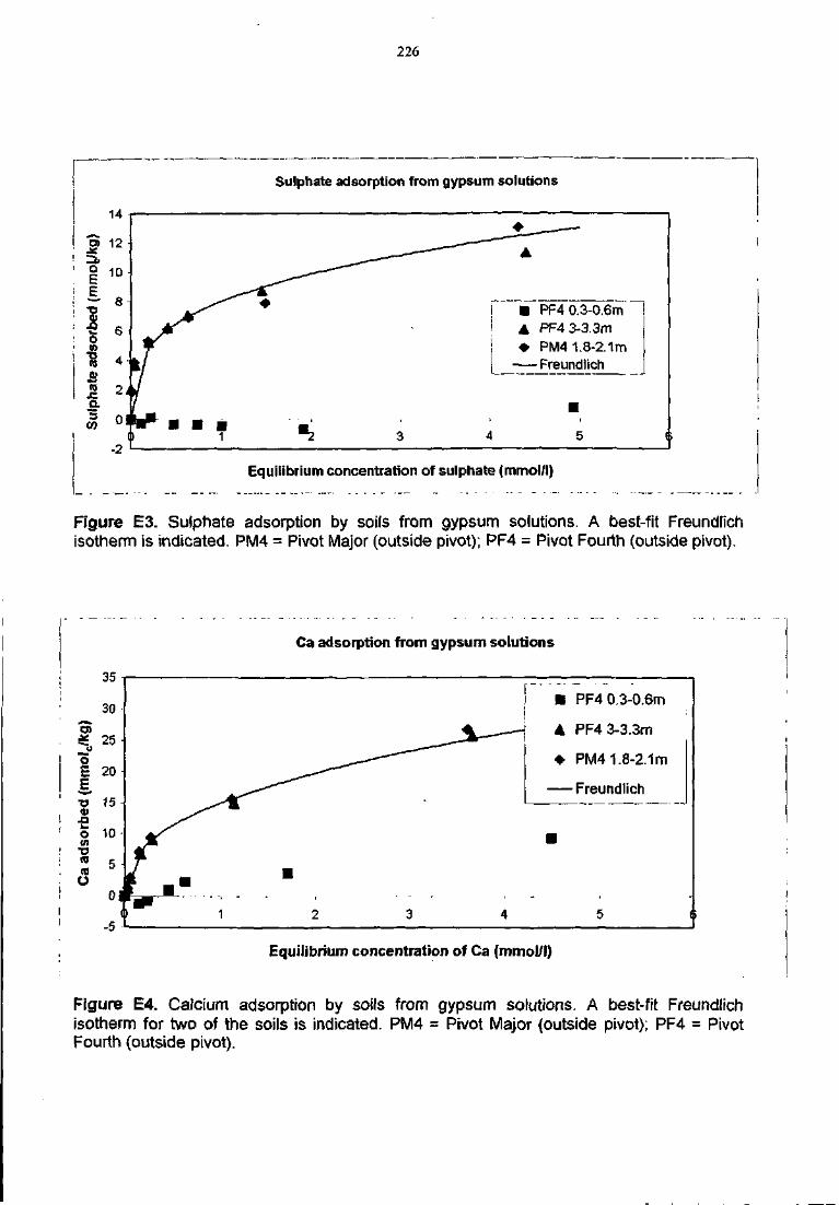
226

Sulphate adsorption from gypsum solutions

14

12

10

f •Ifi!!

2

aI

-2(f> 1 "2

^ —

3

_ — — -

A

•

•

•

PF4 0.3-0.6mPF4 3-3.3mPM4 1.8-2.1mFreundlich

•i

5 1

Equilibrium concentration of sulphate (mmol/l)

Figure E3. Sulphate adsorption by soils from gypsum solutions. A best-fit Freundlichisotherm is indicated. PM4 = Pivot Major (outside pivot); PF4 = Pivot Fourth (outside pivot).

Ca adsorption from gypsum solutions

• PF4 0.3-0.6m

• PF4 3-3.3m

• PM41.8-2.1 m

Freundlich

Equilibrium concentration of Ca (mmol/l)

Figure E4. Calcium adsorption by soils from gypsum solutions. A best-fit Freundlichisotherm for two of the soils is indicated. PM4 = Pivot Major (outside pivot); PF4 = PivotFourth (outside pivot).

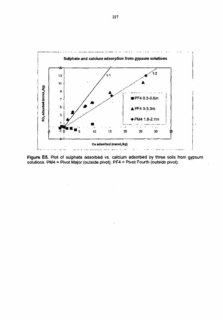
227

O

E

j Is73

o~

Sulphate and calcium adsorption from gypsum solutions

13 -

11 -

9 •

5 •

3

1 --• • - s

3-

/

w -

>• • -) " 5

•10

//

A y^

15

• PF4 0.3-0.6m

APF4 3-3.3m

• PM4 1.8-2.1m

, . - ^- . , - • r- -

20 25 30 3 3

Ca adsorbed (mmol^g)L_

Figure E5. Plot of sulphate adsorbed vs. calcium adsorbed by three soils from gypsumsolutions. PM4 = Pivot Major (outside pivot); PF4 = Pivot Fourth (outside pivot).

Appendix F

Borehole logs

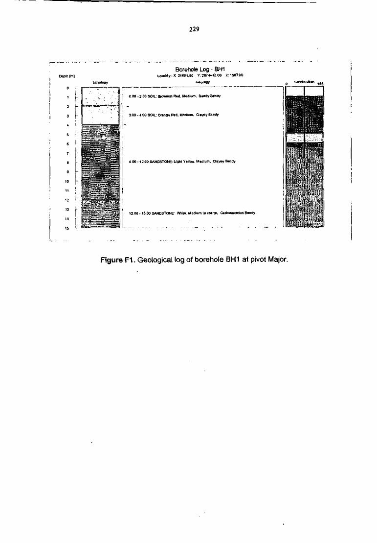
229

Oplh (m]Umoloffy

Borehole Log - BH1Lra l i t y -X 24061.50 TZ674*«,C0 Z:1567flO

Geology

0.00-2.00 SOIL: Brownish Red. Medium, SanOy Sandy

2.00 - f.OO SOIL: Of&nge Red. Medium, Clayey Sandy

4.00 -12.00 SANDSTONE: Llpht Yellow. Medium. Clayey Sandy

12.00 -15.00 SANDSTONE: VkhiK. Medium to CMrs, CalbonaceousSandy

1PiuJJ i:.!,:j

Figure F1. Geological log of borehole BH1 at pivot Major.

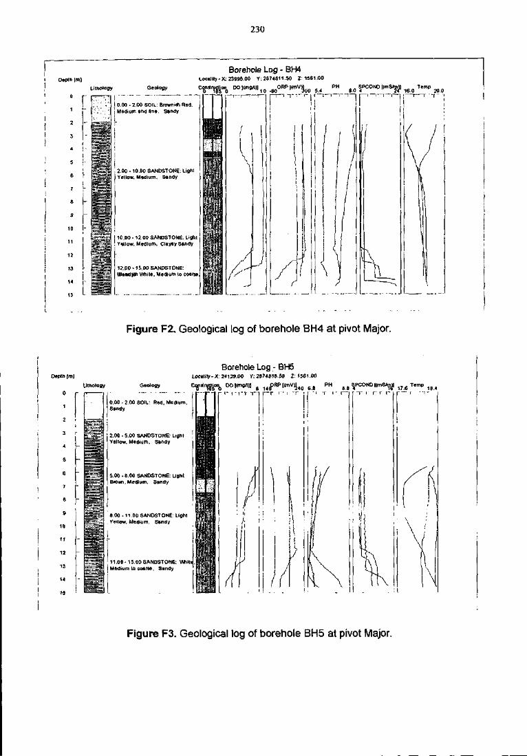
230

I DepWIro]

Borehole Log - BH4Loc.llty-X:2J995,00 Y: 2874811.30 Z: 1361.00

Liltlolo0y Geology

i 0.00 - 2.00 SOIL: Brtnmi* Rod.Medium end flue. Sandy

, 2.00 • 10.00 SANDSTONE: Lightj Yellow. Medium, Sandy

I 10.00 -12.00 SANDSTONE:' Yellow. Medium, Clayey Sandy

1?.00 - IS,DO SANDSTONE:ite, Medium ID coarse,

1 ^ ^ * 2 0 . 0

Figure F2. Geological log of borehole BH4 at pivot Major.

Depth [mj

0

1

2

3

4

5

Uthology Geology

Borehole Log - BH5Locality - * 24123.00 Y: 2S74B1 B.50 Z: 1561.00

00I(mg/l)] B ^pRPKmVH^,, 6 8 PH fl fi |PCOND HmSft̂ a , 7 6 T e m p

9

10

11

12

13

14

ts

r —r i r r r i I r " T -

0.00 • 2.00 SOIL: Red. Medium.Sandy

! 2.00 - 5.00 SANDSTONE: Light 'Yellow, Medium, Sandy

5.00 -8.00 SANDSTONE: LightBrown. Metiium. Sandy

8.00 - 11.00 SANDSTONE: LightYeVfow. Medium, Sandy

11.00-15.00 SANDSTONE:Medium to coarse. Sandy

Figure F3. Geological log of borehole BH5 at pivot Major.

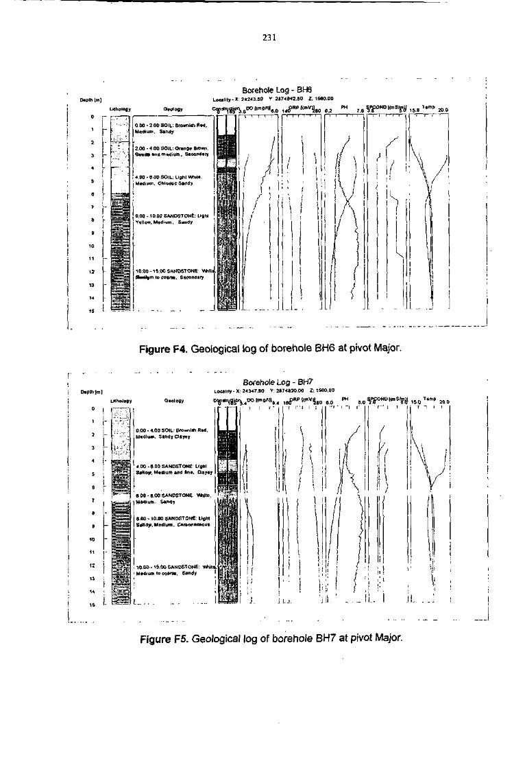
231

Depth [m

Borehole Log - BH6Locality-X:!4243.5P Y: 2474842.50 Z: 1560.00

! 1 Of.' • 6 DC SOIL: Lighl VWiileMedium. Chlpriric Sandy

Figure F4. Geological log of borehole BH6 at pivot Major.

Borehole Log - BH7Locality-X: 24347.50 Y: 2S74HJO.OC Z: ISSD.DO

1 r2

3

4

s

0,00 - 4.00 SOU.: BrawniSi Rsd,Medium, Sandy Clayey

4.00 - 6.00 SANDSTONE: Lighty, Medium and fins. Clayey

8 DO - B.00 SANDSTONE White.

8.00 - 10.00 SANDSTONE:S«»dy, Medium,

10.no-1S.OtiSAMOSTON6-. V*iiie.Medium to co?r«. Sandy '

L...

Figure F5. Geological log of borehole BH7 at pivot Major.

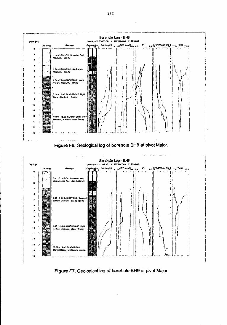
232

Depth Im]

0 |i

1

2

3

4

5

6

Borehole Log - BH8LociSlly - X: 23863.00 V: 16751M.00 Z: 1954.00

Utiolcgy

:

i 0 .00- 3.00 SOIL: Brawi i * Red.! Medium. Sandy

3 Oi l . 5.00 SOIL: Light Brown.Medium, Sandy

5.00 - 7.00 SANDSTONE: LighlYellow, Medium. Sandy

7 0 0 -10.00 SANDSTONE: Ught>wn, Medium, Sandy

10.00- 15.00 SANDSTONE: O«y.|Medium, CartionaKOusSandy j

L ..

Figure F6. Geological log of borehole BH8 at pivot Major.

Depth [ml

0

1

S

3

4

s

s

1

a

g

10

11

12

13

14

15

Lithology Geatogy

COO -3.00 SOIL: UrowmSi Red,Medium ana fine,

Borehole Log - BH9Locality - X: 33S0S.<7 V:2B75147.4a Z: 1554,00

L ! ! = 1 1 I E l

3.00 - 7.00 SANDSTONE: ftrowni^Veliow, Medium. Sandy Stntfy {

7.0O- 13.00 SANDSTONE: Li)tllYellow. Medium. Clayey Sandy ,

13.00 -15.00 SANDSTONE:, Medium to ro

Figure F7. Geological log of borehole BH9 at pivot Major.

Appendix G

Results from pumping test analysis

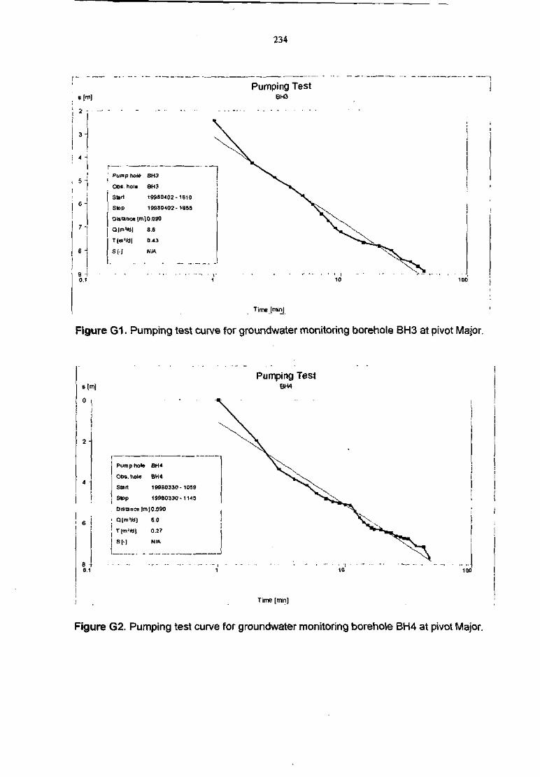
234

s[m]Pumping Test

Bl-O

! 2 I ^ "

3 -

A -

6 "

7 -

rPupip holeOtis hole

I8 -

9 -0.1

Start

Stop

BH3

BH3

19980<02-

19980402-

Distance (m]0.090

Q(rn3/d] 8.6

T[m'/dl

Si-]

0 43

N/A

1610

1655

Timejmin]

Figure G1. Pumping test curve for groundwater monitoring borehole BH3 at pivot Major.

Mm]

2 -

e i0.1

Pump hole BH4

O6S. hole BH4

Start

Stop

1998D330- 1059

199B0330-1145

|0.090

6.0

0.2?

Pumping TestBH4

i ]

ioo

Time [min]

Figure G2. Pumping test curve for groundwater monitoring borehole BH4 at pivot Major.

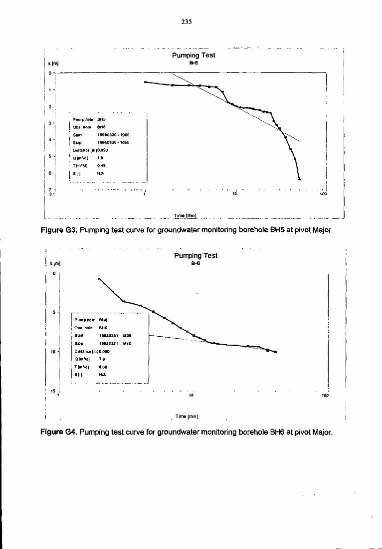
j s[m]

IT

235

Pumping TestBH5

-a .

A -

5 '

6 •

70.1

Pump holeObs. hole

Start

Stop

BH5

6H5

19980330-1000

19920330-1060

Distance [m|0.090

Q[m3MI

'< T[m"/d]

S H

7-8

0 49

N/A

Figure G3. Pumping test curve for groundwater monitoring borehole BH5 at pivot Major.

s[m]

0 i

Pumping TestBH6

5 -

10

Pump hole Bh6

Obs. hole BH6

Start 19980331-1505

S»p 1S9S0331 . 1640

Distance [in]D.090

Olm'WJ 7.8

T [ms/H) 0.68

S [-1 N/A

15100

| Time [min]

Figure G4. Pumping test curve for groundwater monitoring borehole BH6 at pivot Major.

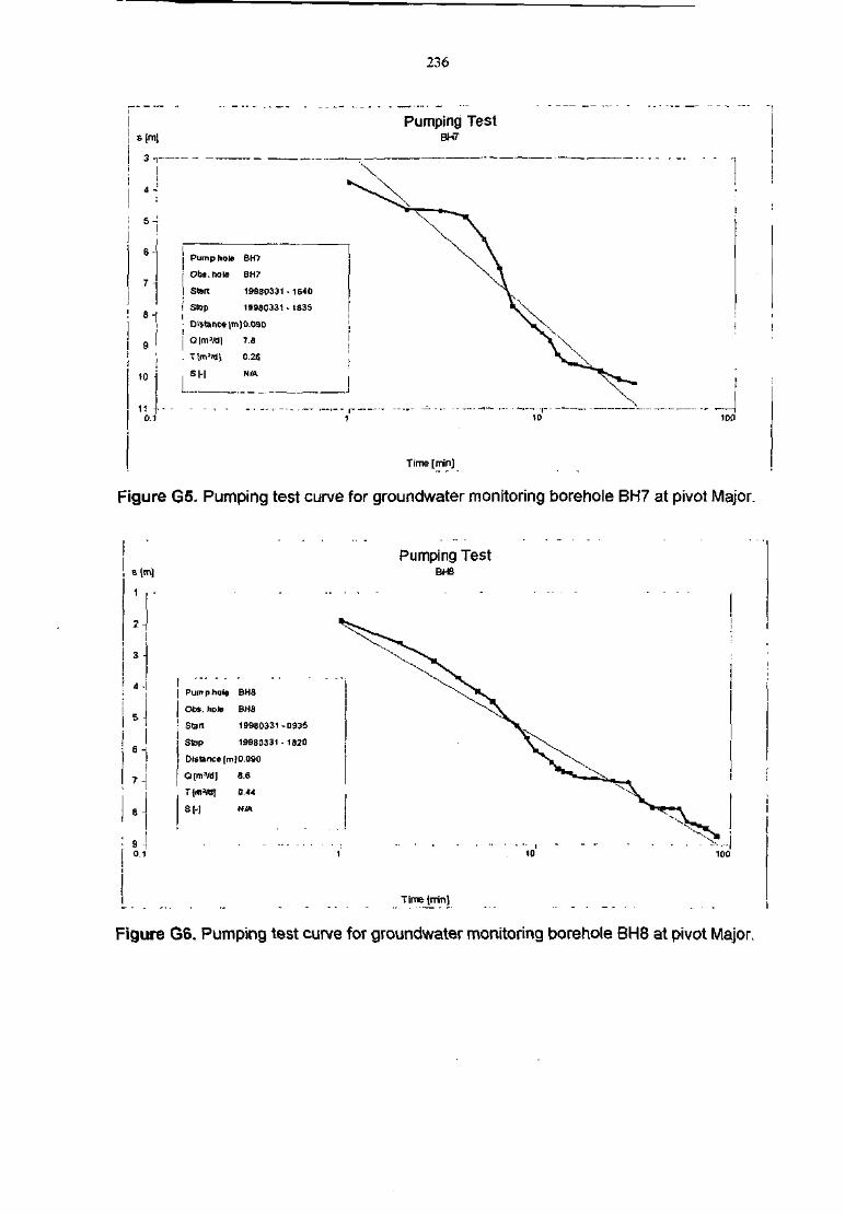
236

Pumping TestBH7

3 -, — ~ — —

5-

6-

7

i 9

10

110.1

I Pum p hole BH7

ObS.hole

Start

Stop

BH7

19980331-1640

19980331 -183S

Distance |m)O.0SD

Q|m3AJ]

T \m'»\

Sl-I

7.8

0.26

N/A

100

Time [rrin)

Figure G5. Pumping test curve for groundwater monitoring borehole BH7 at pivot Major.

Puntptiole BH8

Obs. hole BUS

• Start 19980331 -0935

j Stop 199BD331 - 1820

Distance [m|0.090

Q im'rtl] 8.6

0,44

Pumping TestBH8

100

Tirne(rrin]

Figure G6. Pumping test curve for groundwater monitonng borehole BH8 at pivot Major.

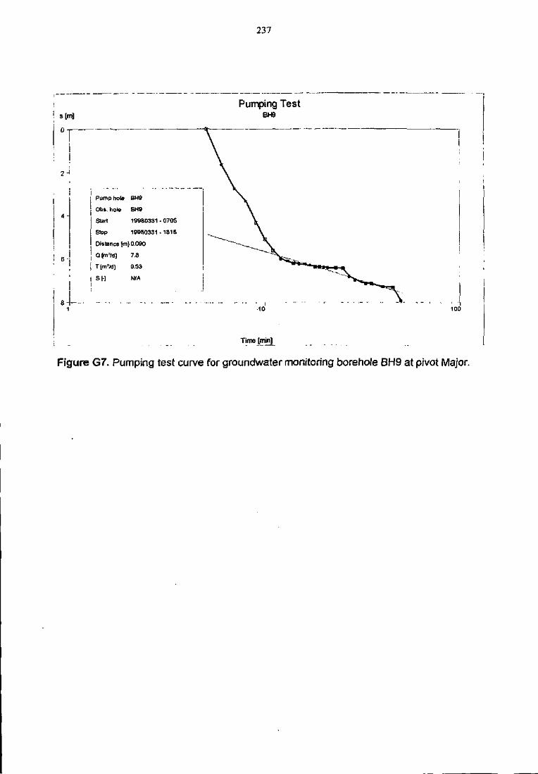
237

s[m]

i 6

• 4 - .

Pumping TestBH9

Pump hole BH8

Obs. hole BH9

Start 1998D331-070S

Stop 19980331-1815

Distance [m) 0.090

j Qinrtd] 7.8

j Tjm=/d] 0-53

| SH N/A

100

Time [min]

Figure G7. Pumping test curve for groundwater monitoring borehole BH9 at pivot Major.

Appendix H

Solute transport characteristics breakthroughcurves

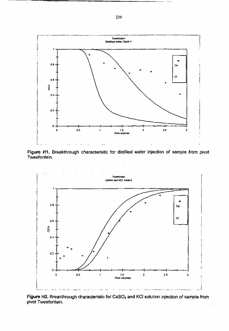
239

0,5

TweefonteinDlsWtwS water. Cycle 1

o.a -

D.6 -

0.4 -

0.2-

0 -

: \

1 1 1—

• \ .

^ ^ — - — .

—I 1 1 1

*

Ca

Cl

I . 1 1

1.5Pore volumes

2,5

Figure H1. Breakthrough characteristic for distilled water injection of sample from pivotTweefontein.

Tweefontein

CaSCM and KCI: Cycle 2

0.8 -

0.6 -

0.4 -

0.2 -

0 -

; / .

• / /

/ /

1—.^ i 1 1 1——1 1 1 1—

•

Ca

Cl

—1

0.5 1 1.5 2Pore volumes

2.5

JFigure H2. Breakthrough characteristic for CaSO4 and KCI solution injection of sample frompivot Tweefontein.

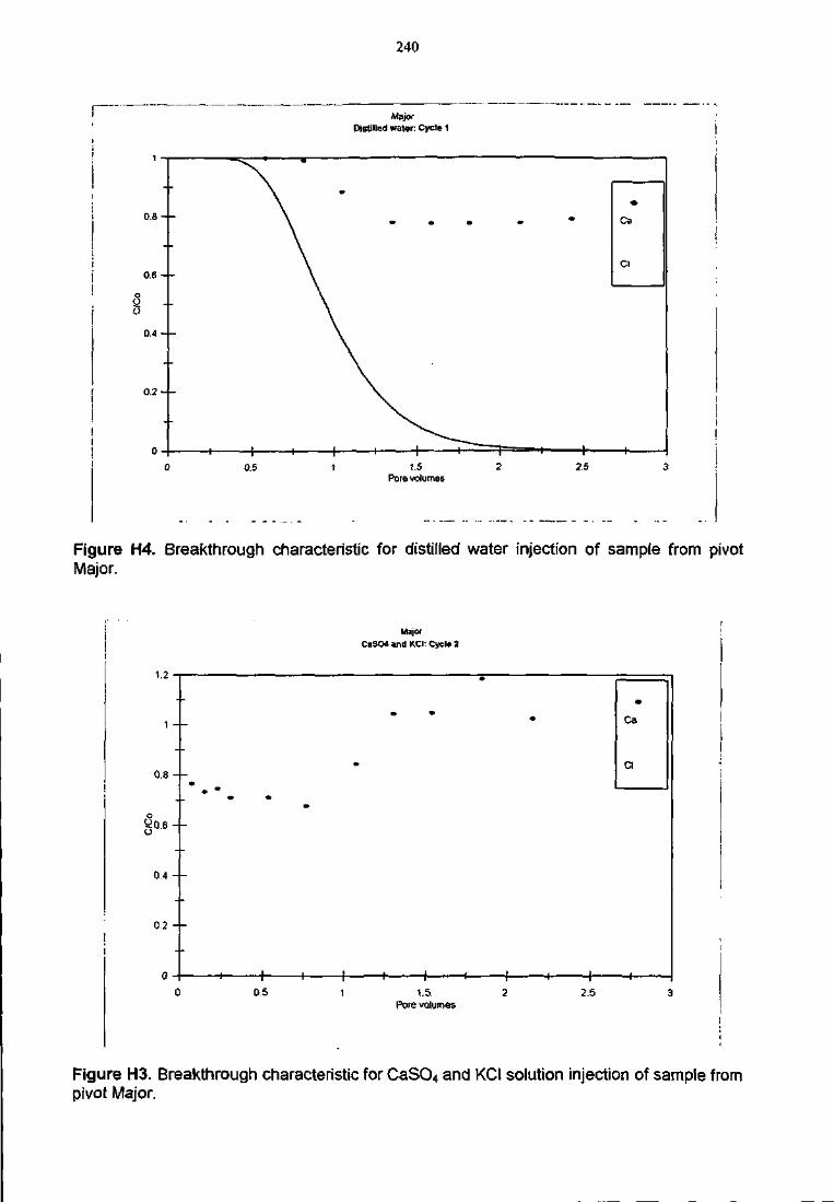
0.5

240

MajorDistilled water. Cycle 1

0.8 -

0.6 -

0.4 -

0.2 -

0 - 1 1

\ '

\

\

1 1 1 1 1 1* t— 1 1

•Ca

Cl

—1

1.5 2Pore volumes

2.5

Figure H4. Breakthrough characteristic for distilled water injection of sample from pivotMajor.

MajorCaSCM and KCl: Cycle 2

1.2

1 - -

0.8 - -

l O . t - -

0,4 - -

0.2 - -

H 1 K -I 1 K

Ca

0.5 1.5.Pore volumes

2.5

Figure H3. Breakthrough characteristic for CaSO4 and KCl solution injection of sample frompivot Major.

APPENDIX I

Chemistry of soils and regolith irrigated withgypsiferous mine water

242

Introduction

A characterization of the effects on soil and deep sub-soil chemistry of irrigation withgypsiferous mine water at Kieinkopje was conducted by Ross Campbell and Prof. Martin Fey atthe Universities of Cape Town and Stellenbosch. The methods used to analyze deep soilsamples and the results of these analyses are presented in this Appendix.

Methods

Soil samples from the areas irrigated to field capacity in pivots Major, Fourth and Tweefontein,as well as samples of non-irrigated soil close to each pivot were examined. Certain sub-samplesrepresenting particular depth intervals have been omitted to save analytical time, but these gapsin the data do not appear to mar the clear trends apparent in the majority of results obtained.Samples from the leaching fraction and deficit treatment irrigation areas have not beenconsidered in this report.

Soil passing through a 2 mm sieve has been analysed using the methods discussed below. Thefollowing analytical procedures have been performed:

a) Saturated paste extracts

Electrical conductivity of extracts, major cations and anions by ion chromatography, alkalinity ofextracts by titration and dissolved organic carbon.

b) PH

Soil pH has been measured in the saturated pastes and in 1:2.5 soil suspensions in water and1M KCl.

c) Exchangeable cations

Exchangeable acidity by extraction with 1M KCl and titration against 0.01 M NaOH. Ammoniumacetate extracts analysed by atomic absorption spectroscopy for exchangeable Ca, Mg, Na andK.

d) Colloid mineralogy

Clay fraction mineral identification by X-ray diffractometry (XRD).

e) Textural analysis

Separation and determination of relative proportions of sand, silt and clay by sieving andsuspension in sodium hexametaphosphate solution.

f) Organic carbon

Total organic carbon content of the soils by the Walkley-Black dichromate oxidation method.

243

Major findings

1. Saturated paste extract analyses revealed soluble salt accumulation in the irrigated soilsgreatly in excess of soils not treated with gypsiferous mine water.

2. In pivot Major, most soluble salts were confined to the upper 1 m, while in pivot Fourth therewas a more uniform distribution of salts in the profile, with a slight peak between 1.5 and 2mdown in the profile.

3. In pivot Major ammonium acetate extractabie cation data (an index of exchangeable cationconcentration) revealed a decrease in adsorbed Ca with depth, and a significant increase inadsorbed Mg with depth, with the extractable Mg concentration exceeding that of Ca below1.2 m.

Results

See the following pages for selected analytical results.

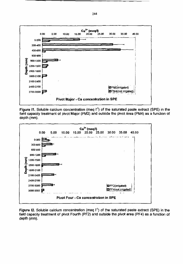
244

E

Dep

i

0.00

0-200

200-400

400-600

600-900

900-1200 \r-nr

1200-1500 P ^

1500-1800

1800-2100

2100-2400

2400-2700

2700-3000

F*

Ca2+ (meq/l)5.00 10.00 15.00 20.00 25.00

-•"• " I — 1 — •

Pivot Major - Ca concentration

30.00 35,00 40

DPM2(imgated)DPM4(nqt irrigated) j

in SPE

.00

Figure 11. Soluble calcium concentration (meq I'1) of the saturated paste extract (SPE) in thefield capacity treatment of pivot Major (PM2) and outside the pivot area (PM4) as a function ofdepth (mm).

Ca2+ (meq/l)0.00 5.00 10.00 15.00 20.00 25.00 30.00 35.00 40.00

L .

| 1200-1500

^T 1500-1800 [p«

§• 1800-2100 IQ

2100-2400

2400-2700

2700-3000

3000-3300

|DPF2(irrifiated)[DPF4(not irrigated)

Pivot Four - Ca concentration in SPE

Figure 12. Soluble calcium concentration (meq I"1) of the saturated paste extract (SPE) in thefield capacity treatment of pivot Fourth (PF2) and outside the pivot area (PF4) as a function ofdepth (mm).

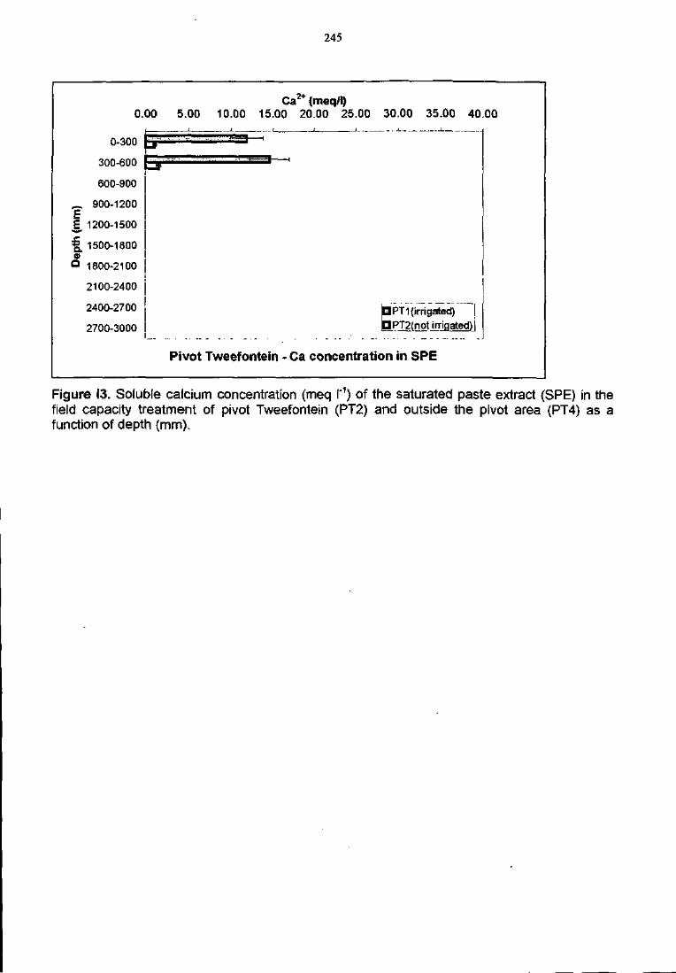
245

£

fa

0.00

300-600

600-900

900-1200

1200-1500

1500-1800

1800-2100

2100-2400

2400-2700

2700-3000

h1

bar

Ca2+ (meq/l)5.00 10.00 15.00 20.00 25.00 30.00 35.00 40

QPT1 (irrigated)DPT2(not irrigated)!

00

Pivot Tweefontein - Ca concentration in SPE

Figure 13. Soluble calcium concentration (meq I*') of the saturated paste extract (SPE) in thefield capacity treatment of pivot Tweefontein (PT2) and outside the pivot area (PT4) as afunction of depth (mm).

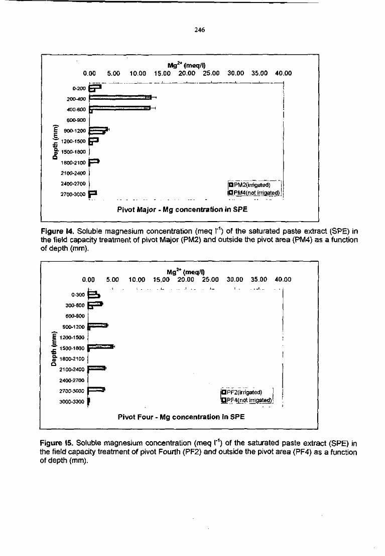
246

E

0.00

0-200

200-400

400-600

600-900

900-1200

1200-1500

1500-1800

B="

*~

1800-2100 p ^

2100-2400

2400-2700

2700-3000 r=»

Mg2+ (meq/l)5.00 10.00 15.00 20.00 25.00 30.00 35.00 40.00

|

JQPM2(irrigated)~" "IinPM4(natJrrigated)J

Pivot Major - Mg concentration in SPE

Figure 14. Soluble magnesium concentration (meq I'1) of the saturated paste extract (SPE) inthe field capacity treatment of pivot Major (PM2) and outside the pivot area (PM4) as a functionof depth (mm).

Dep

th

0.00

0-300

300-600

600-900

900-1200

1200-1500

1500-1600

1800-2100

2100-2400

2400-2700

2700-3000

3000-3300

S i

r =

i

Mg2+ (meq/l)5.00 10.00 15.00 20.00 25.00 30.00 35.00 40.00

a<

h

OPF2{irrigated) JnPi41nqt irrigated).!

Pivot Four - Mg concentration in SPE

Figure 15. Soluble magnesium concentration (meq I"1) of the saturated paste extract (SPE) inthe field capacity treatment of pivot Fourth (PF2) and outside the pivot area (PF4) as a functionof depth (mm).

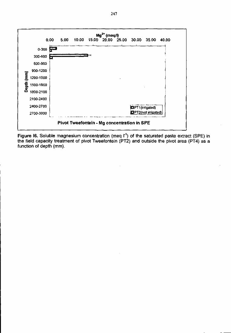
247

t

spth

Q

0.00

0-300 g 3

300-600

600-900

900-1200

1200-1500 ;

1500-1800

1800-2100

2100-2400

2400-2700

2700-3000

Mg2+ (meq/l)5.00 10.00 15.00 20.00 25.00 30.00 35.00 40.00

In PT1 (irrigated) 1ID PT2(not irrigated)!

Pivot Tweefontein - Mg concentration in SPE

Figure 16. Soluble magnesium concentration (meq I'1) of the saturated paste extract {SPE) inthe field capacity treatment of pivot Tweefontein (PT2) and outside the pivot area (PT4) as afunction of depth (mm).

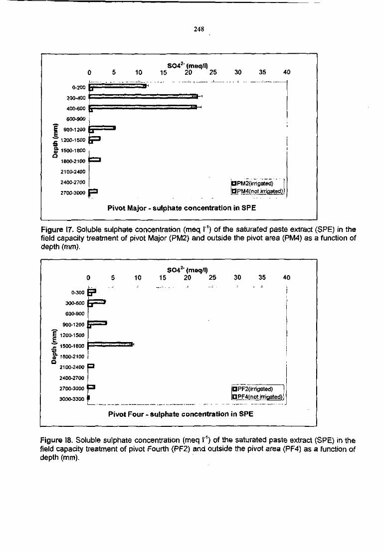
248

E,

Dep

i

(

0-2QO

200-400

400-600

600-900

900-1200

1200-1500

1500-1800

1800-2100

2100-2400

2400-2700

2700-3000

)

" -

* * •

5=or-1

— I

SO42 ' (tneq/l)5 10 15 20 25 30 35 40

' 1I

i

JaPM2(irrig'ated) "|nPM4(not irrigated).

i

Pivot Major - sulphate concentration in SPE

Figure 17. Soluble sulphate concentration (meq I"1) of the saturated paste extract (SPE) in thefield capacity treatment of pivot Major (PM2) and outside the pivot area (PM4) as a function ofdepth (mm).

E

Dep

th

(

0-300

300-600

600-900

900-1200

1200-1500

1500-1800

1800-2100

2100-2400

2400-2700

2700-3000

3000-3300

SO4) 5 10 15

|SS3

a

i

Pivot Four - sulphate

2" (meq/f)20 25

concentration

30 35 40

- ~

i

i

QPF2(irrigated)nPF4(not irrigated)!

nSPE

Figure 18. Soluble sulphate concentration (meq I"1) of the saturated paste extract (SPE) in thefield capacity treatment of pivot Fourth (PF2) and outside the pivot area (PF4) as a function ofdepth (mm).

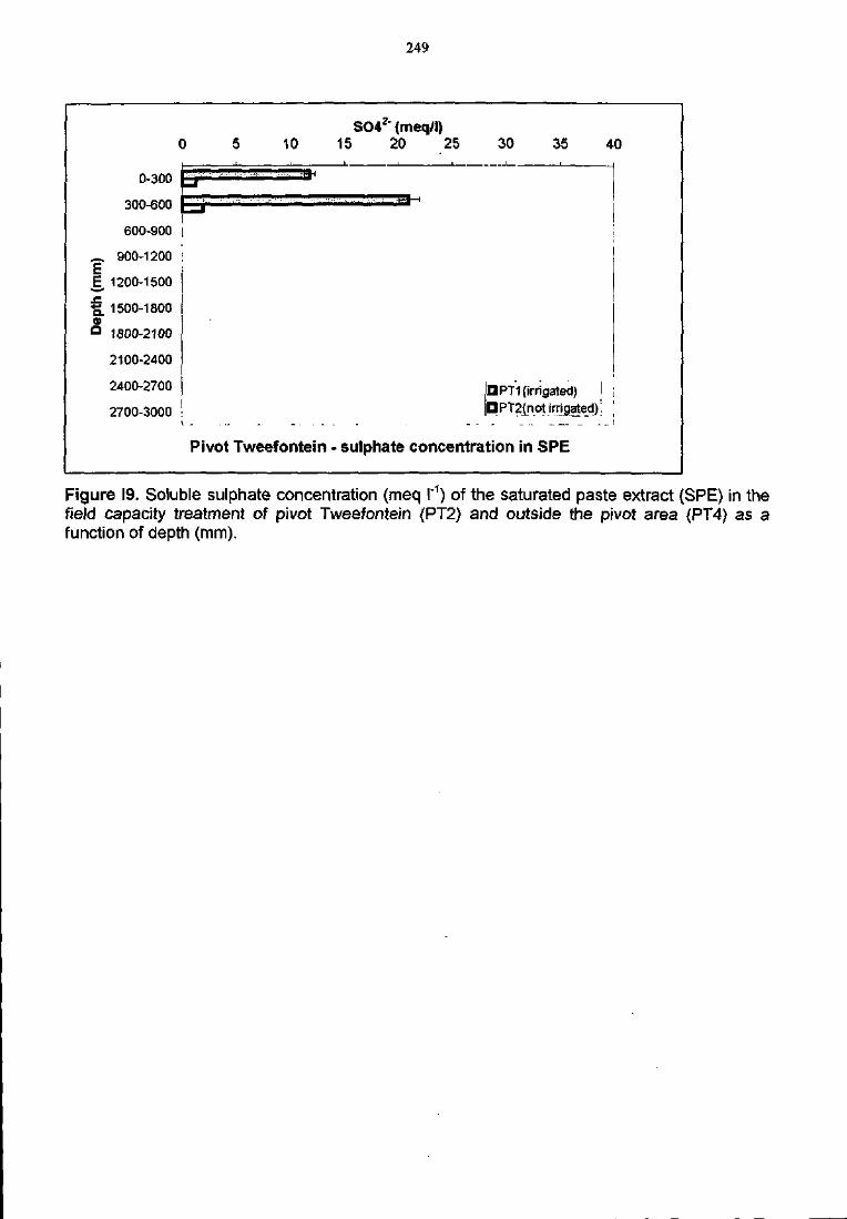
249

(mm

)

UQ

(

0-300

300-600

600-900

900-1200

1200-1500

1500-1800

1800-2100

2100-2400

2400-2700

2700-3000

)L

= J

L _ . . .

Pivot

SO42" (meq/1)5 10 15 20 25 30 35 40

QPT1 (irrigated) ;DPT2(not irrigated); [

Tweefontein - sulphate concentration in SPE

Figure 19. Soluble sulphate concentration (meq I"1) of the saturated paste extract (SPE) in thefield capacity treatment of pivot Tweefontein (PT2) and outside the pivot area (PT4) as afunction of depth (mm).

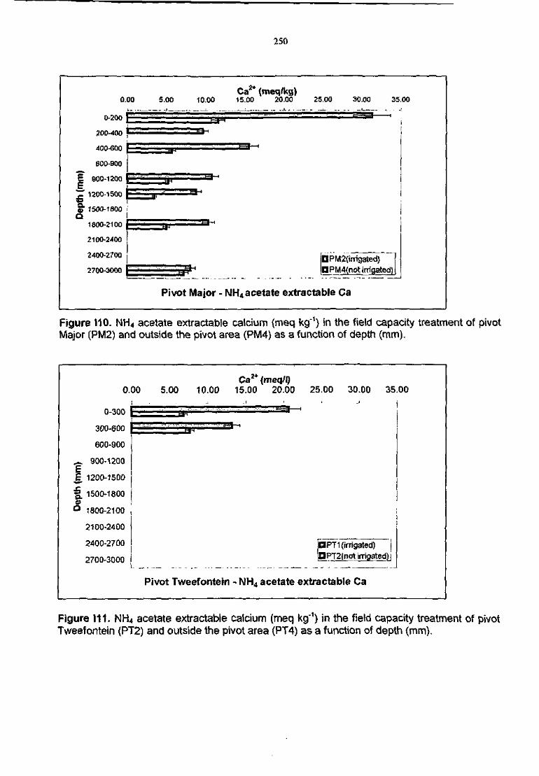
0.00

0-200 £

200-400 p

400-600 P

600-900 |

E 900-1200

" 1200-1500

(f 1500-1800Q I

1800-2100 t

5.00 10.00

250

Ca2+ (meq/kg)15.00 20.00 25.00 30.00 35.00

2100-2400 [

2400-2700

2700-3000 I ' "••••••MM-i^ljfifr'

|BPM2(imgated)D PM4(not irrigated)]

Pivot Major - NH4acetate extractabie Ca

Figure 110. NH4 acetate extractabie calcium (meq kg'1) in the field capacity treatment of pivotMajor (PW12) and outside the pivot area (PM4) as a function of depth (mm).

0.00

0-300

300-600

600-900

^ 900-1200£

B. 1200-1500

f_ 1500-1800

° 1800-2100

2100-2400

2400-2700

2700-3000

5.00Ca2+ (meq/l)

10.00 15.00 20.00 25.00 30.00 35.00

i

Pivot Tweefontein - NH4 acetate extractabie Ca

Figure 111. NH4 acetate extractabie calcium (meq kg"1) in the field capacity treatment of pivotTweefontein (PT2) and outside the pivot area (PT4) as a function of depth (mm).

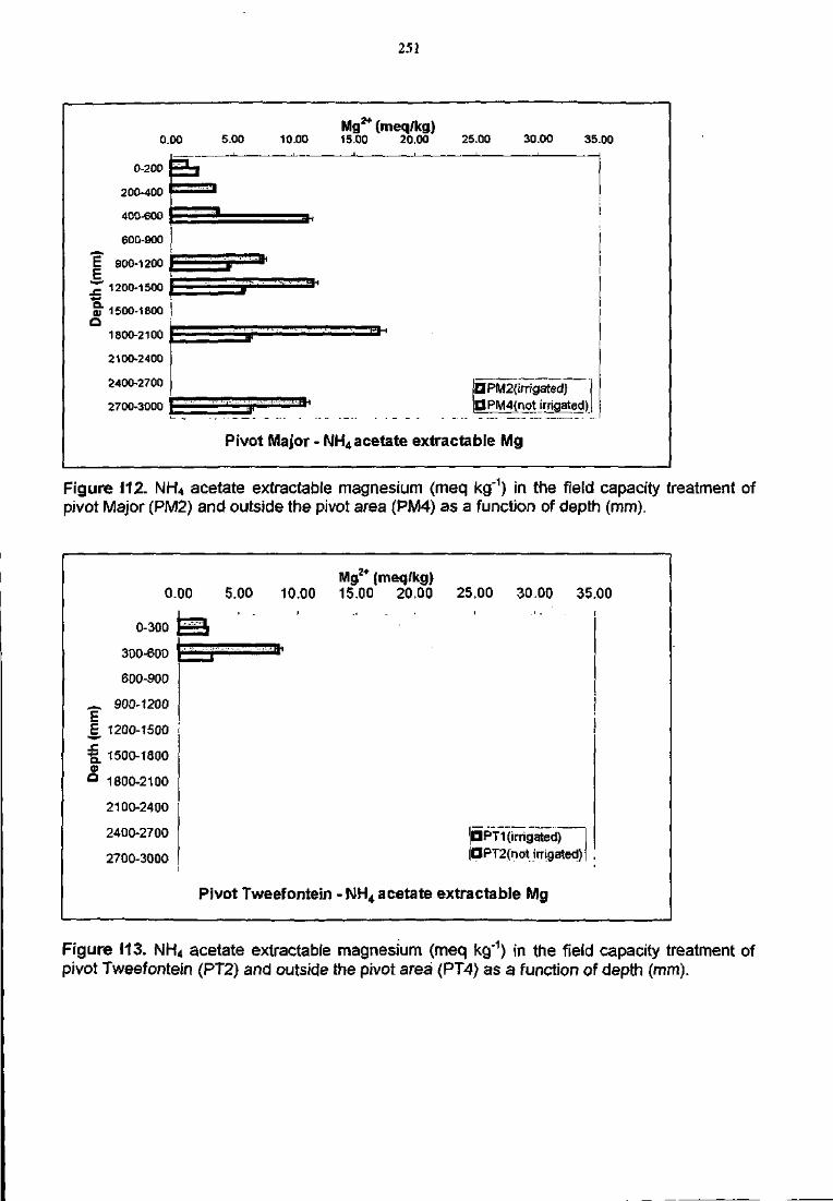
0.00

D-200

200-400

400-600

600-900

E 900-1200 £E >]T 1200-1500 K

S" 1500-1800 IQ

1800-2100

2100-2400

2400-2700

2700-3000

5.00 10.00

251

Mgz+ (meq/kg)15.00 20.00 25.00 30.00 35.00

QPM2(irrigated)|DPM4(notjiTigated)

Pivot Major - NH4 acetate extractable Mg

Figure 112. NH4 acetate extractable magnesium (meq kg"1) in the field capacity treatment ofpivot Major (PM2) and outside the pivot area (PM4) as a function of depth (mm).

(mm

)jp

th

a

0.00

0-300

300-600

600-900

900-1200

1200-1500

1500-1800

1800-2100

2100-2400

2400-2700

2700-3000

Mg2+ (meq/kg)5.00 10.00 15.00 20.00

m • '

Pivot Tweefontein - NH4 acetate

25.00 30.00 35.00

QPTIOrrigated) 1a PT2(not irrigated)'

extractable Mg

Figure 113. NH4 acetate extractable magnesium (meq kg'1) in the field capacity treatment ofpivot Tweefontein (PT2) and outside the pivot area (PT4) as a function of depth (mm).

Appendix J

Results of chemical analyses of borehole watersamples

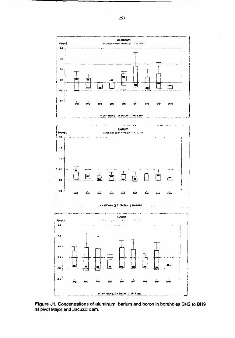
253

AluminumAl(mo/L]

' 0.6

JL

— i —

i—

0.0

B H B B H 3 B W B H 5 B M 6 B H 7 B H & B H 9 CWM

Barium! Baimg/L)I

2.0

t.5

0.5

0.0

•0.5 i

, LastVSlue (1 2iadDcv | M n t H s

Boron

iSjBne/LJ

2.0

0.5 -

0.0 +

-0.5BH2 6H3 BH( BH)

iSta0ev.

BHB B-B DftM

Figure J1. Concentrations of aluminum, barium and boron in boreholes BH2 to BH9at pivot Major and Jacuzzi dam.

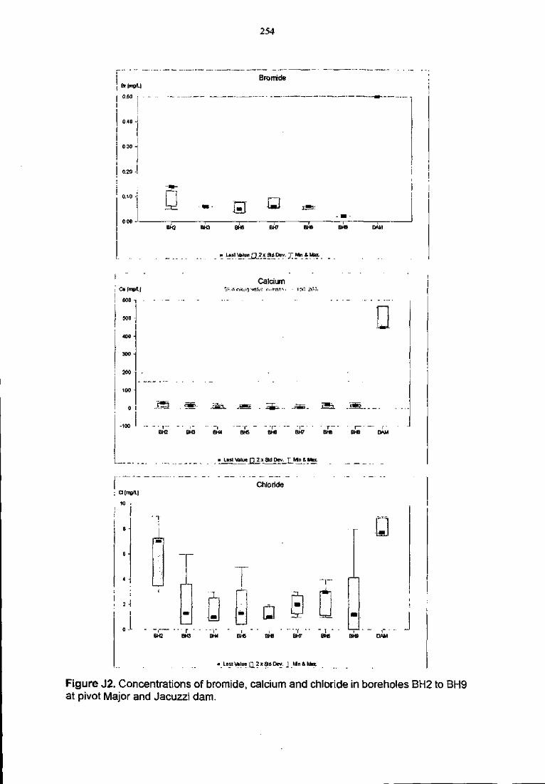
j Br|mg>Ll

| 0.H , •

0.40

|j 030

0.20 -

254

Bromide

BH2 8H3 BH6 BH7 BHS BH9 BAM

LBSI \ftJue_Q_2 X 3d Dev. j ; Mn * Max

i i

600

300 -

] 200

too

0 I

-100 '

i

Calcium

BHJ BH« BHS 6H6 BH7

Chloride

I 2 -j

I I

D

BHB

3 a

BH9 DAM

a e8H2 BH4 BH5 EH6 BH7 BHS

a

BH9 DfiM

• LsstUiliicQ2xa(lDev. T Mn&htax.

Figure J2. Concentrations of bromide, calcium and chloride in boreholes BH2 to BH9at pivot Major and Jacuzzi dam.

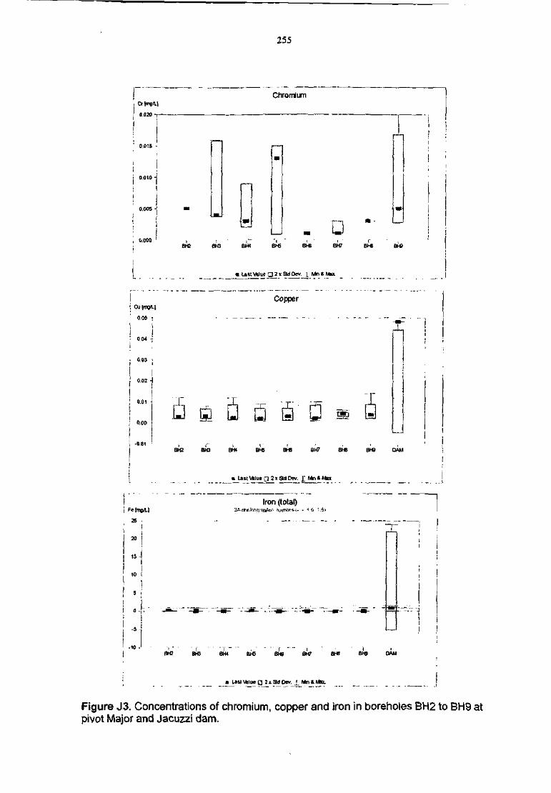
255

Chromium

0.02O -r

0.005 -'

00M

L .

0.05 i

• 0 . 0 4 •;

• 0 . 0 3 >

| 0 0 H! Ii 0.00

f e

2 5 •

I 15

0 .

-s

.10 -

0BH2 6H3 BM4 BH5 BH6 BH8

i La«\rtiUiea2xadDev, 1 MniMax.

Copper

S

Iron (total)

Eht)

B H 2 B t O B H 4 B H S B H 6 B H 7 B H 3 B H 9 CAM

I I

BH2 EH3 BH4 BH5 BHS BK? EH8 0AM

• Last Value Q I i 3tf Dcv. 1 Mn 4 Mat

Figure J3. Concentrations of chromium, copper and iron in boreholes BH2 to BH9 atpivot Major and Jacuzzi dam.

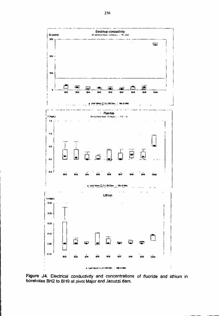
256

£C(m3tnJ

300 -T

Electrical conductivity

. 200

100

! i! 0 L-

DH3BH3 BH* BHS BH6 BH7 BHB BH9 DAM

• laWUdlueQ2*S0C>ev. | Mni.Wai

F[mgn.]

1.5

1.0

0.S •

-0.5

0.30 •

i -0.10

0.20

0.10 -

O.OO

I

~ "

Fluoride

y a..fi.fl 0BH2 BN3 BH4 BH5 BH3 BHT BH6

• LdSIVSIueQ 2 iadDev. I Un & Max.

Lithiun

1=1 J33:

BH3 6K3 BH4 BH5 B« BH7 BHB BH9 DAM

t Lesi VBiuf I i 2 < 3d Oev :

Figure J4. Electrical conductivity and concentrations of fluoride and lithium inboreholes BH2 to BH9 at pivot Major and Jacuzzi dam.

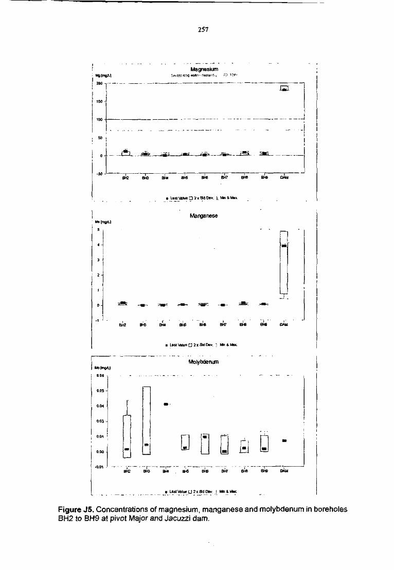
257

Magnesium

I 150 -!

-so J

i

" I! i

B H 2 B H 3 B H 4 B H 5 B H 6 B H 7 B H 8 B H 9 DAM

• List \Mue • 2 « S i Dev. ] . Whi & Max

rMo[mg/l.f

Manganese

BH2 BH3• r

BH4

Wfoiybdenum

0.05 -

0.0*

0.0S -

O.O1

0,00

1

1

— •

t

BH5 SH8 BH7 EH8 BHS EMM

. I Mn 8. Max

BH2 BK3—J—

BH4 BH5 BHB BUT BH> B H 9 D A M

• Lasl\Alu«U2xadOev. J Mni.Mu.

Figure J5. Concentrations of magnesium, manganese and motybdenum in boreholesBH2 to BH9 at pivot Major and Jacuzzi dam.

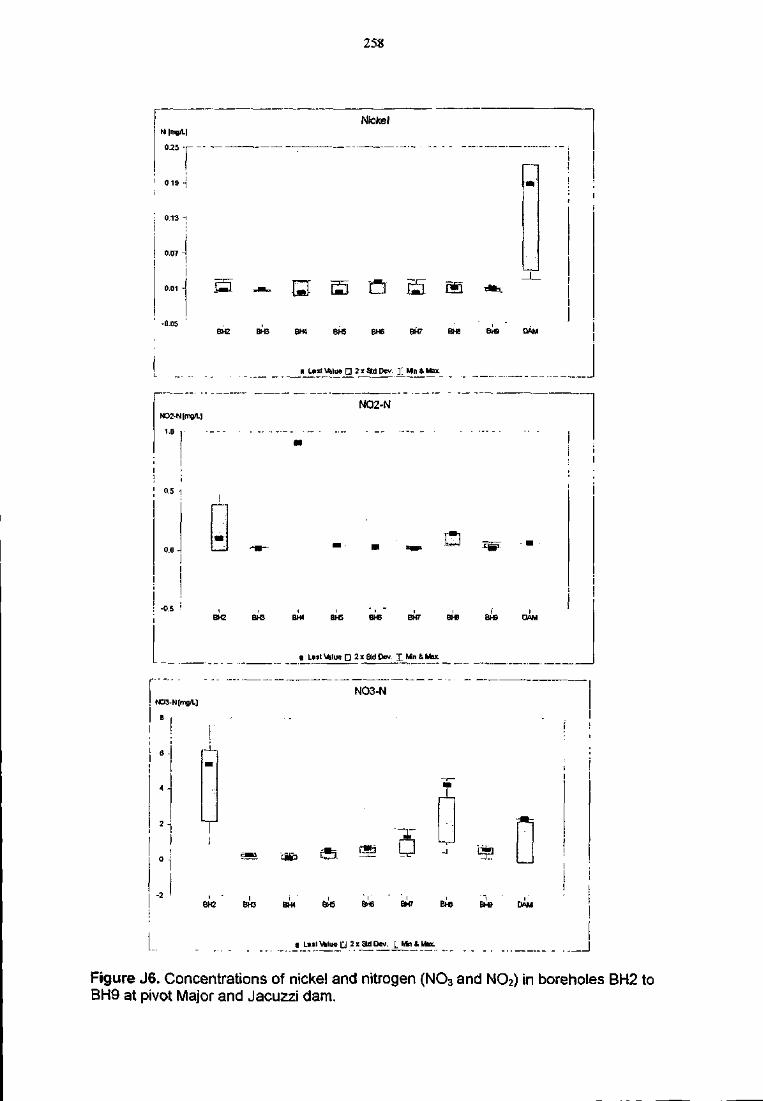
258

0.25 r• 0.13 -

0.07

-0.05

Nickel

ND2-N|mg/L!

1.0 T-

B H 2 B H 3 B W B H 5 B H 6 B H 7 B H 8 B H 9 DAM

i Last Wilue • 2 x Sd Dev. X Wn » Max.

NO2-N

I °-5 1

o.o •

I

• -0.5 'B H 4 B H S e H 6 B H 7 B H 8 a H 9 QAM

• Last\61ueO 2«adDev. I MntMax

! NO3-N[mg/l]NO3-N

T

BH2 BH3 BH4 BH5 BHB BH7 BH6 BH9 DAM

I I

| • Last\61uep 2 x ^ D e ^ j._Mn & Max. J

Figure J6. Concentrations of nickel and nitrogen (NO3 and NO2) in boreholes BH2 toBH9 at pivot Major and Jacuzzi dam.

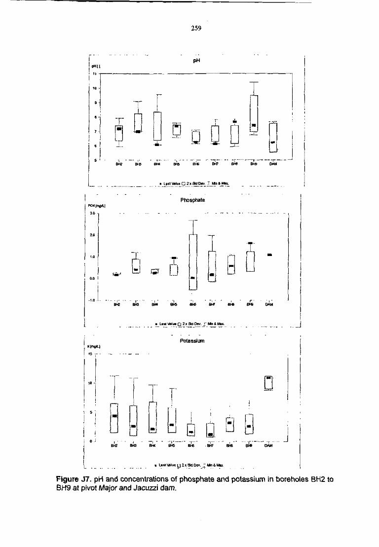
259

PH! PHU

7 -I

I

•6H2 BH3 BH4 BHS BH6

—j —

BH7

T

BHS BHS DAM

• LBSt Vfclue • 2 x a o Dev. J Mn i Max.

I Q.Q !

- 1 . 0 - 1 - - • -

Phosphate

D

T

• - I " ' - - " I " • • - 1 " • " I " I " [ • r " T " " " I "

BH2 BK3 EH< BHS B H S 6 H 7 EH8 6H9 WVM

• Last Wlue Q 2 x 3 0 Dev. r Mn » M31.

! 15 T -

10 -

I !o - I

Potassium

T T

BW BH3 BH4 BHS BHE • BH7 BHB EU« DAM

u 2 x SW Oev. ~

I

Figure J7. pH and concentrations of phosphate and potassium in boreholes BH2 toBH9 at pivot Major and Jacuzzi dam.

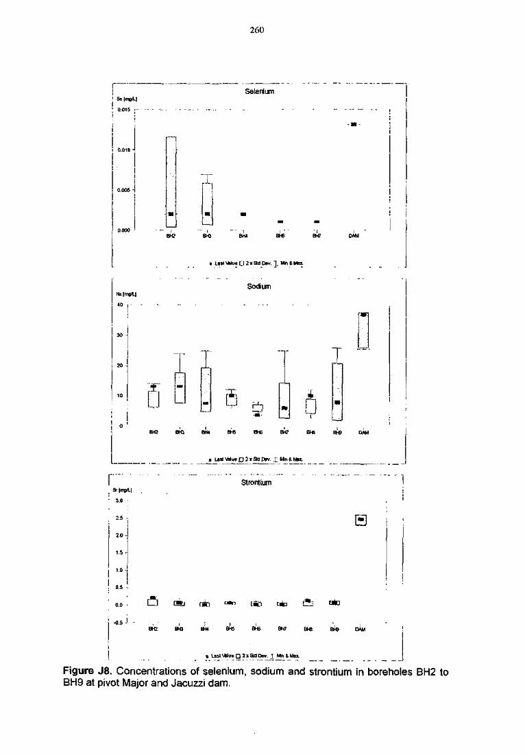
260

0.000

Naimg/LJ

40 i

20 -

Selenium

BH2 BH3 BH4 8H7

• L»s!\*iu«G2iadDev. 1

Sodium

I £ I

EH3 BK5 BH4 BH5 BHE BW BUS BK) DAM

I i las;i las;MMueQ2x3aDev. j

Strontium

J 3.0

2.5

2 0 -

1.5 -

I 1 °.I 0.5

0.0

-0.5

LJ

B H 2 B H 3 E H 4 B H 5 B H S B H 7 B H 8

Last\&lueQ2>;adDcv. J MniMax.

BH9 DAM

Figure J8. Concentrations of selenium, sodium and strontium in boreholes BH2 toBH9 at pivot Major and Jacuzzi dam.

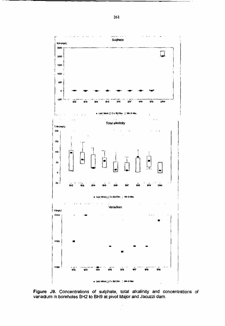
261

j S04!ms<L.J

2500 T

1500 •

1000 ;

0 -I :-»= «•»-.

Sulphate

-500 - J - . r , , - , —BK5 BH4 BH5 BH6 BH7 BH9 DAM

• Las! \fclue l-II 2 i 3 d Dev _• Mn 4 Mat

Total alkalinity

200

150

100 -

50

"[

i

• 4 - , 1

d D W s Q- 5 0 -̂ • J - — I • i J j" "" I i

BH2 BKJ BH4 BH5 BHB BH7

e | J 2x30Dev. j Mn 4 M9i

0 010

O.00S

~BH2~

VanacSum

3!» 6H5 BH6 BW BHB

• Las! Mlue U 2 x 3 d Dev. ; Mn & Htax

Figure J9. Concentrations of sulphate, total alkalinity and concentrations ofvanadium in boreholes BH2 to BH9 at pivot Major and Jacuzzi dam.

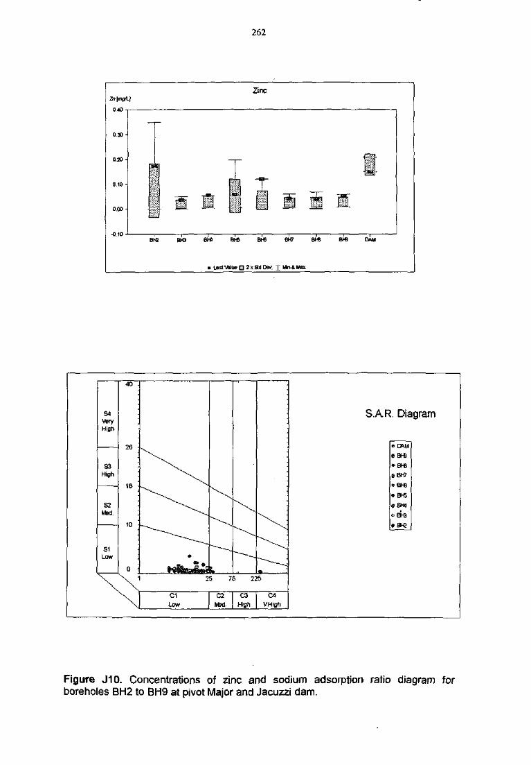
262

B H 3 B H f B H 5 B H 5 B H 7 B I * B H 3 C W M

B UJStVilue ED 2xSdDev. j Mn&Max

S4VeryHigh

S3High

S2Wted.

S1Low

\

40 -

18 -

0 1

^ \

" - — ^

•

-

•

^ ^ ^ •

^ V 1 25 75 225

X' C1

Low

C2

Msd.

C3

High

C4

VHigh

SAR. Diagram

eBH)

*BH5

eBH?

oB-6• H-6

* B H 2

Figure J10. Concentrations of zinc and sodium adsorption ratio diagram forboreholes BH2 to BH9 at pivot Major and Jacuzzi dam.

APPENDIX K

Growth and nutrient composition of Triticumaestivum L. as affected by nutritional management

under sulphate salinity

264

Introduction

Accumulation of salts in the root-zone can adversely affect plant growth due to a loweredosmotic potential, caused by the high concentration of soluble ions, specific ion toxidties(Grattan and Grieve, 1994) or nutritional imbalances (Bernstein et al., 1974). Most cropplants have evolved under conditions of low soil salinity and consequently have developedmechanisms for absorbing nutrients in non-saline soil. The utilization of soils containingexcessive amounts of Ca, Mg and SO4 raises the problem of providing growing conditionsthat will support reasonable plant productivity. Mashali (1996) reported that highconcentrations of Ca and SO4 in the soil solution could decrease the plant uptake of K, Mg,Mn, Fe, Cu, Zn, PO4 and NO3 through ion competition and complementary ion effects onnutrient uptake. High concentrations of Ca and Mg in the soil solution may lead to asubstantial release of K from the adsorption complex with a possible loss through deeppercolation under leaching. Excessive amounts of gypsum in the active root-zone may alsoaffect nutrient availability and uptake by plants (Mashali, 1996). The precipitation ofphosphate ions and fixation of micronutrients in an unavailable form seems to be the mostcompelling problems associated with excessive gypsum in the soil (Panahi and Rowell,1996; Mashali, 1996; Oyonarte et al., 1996). Excessive gypsum may further cause loss ofnutrients through cation and anion interaction effects (Mashali, 1996; Fey et al., 1997).

If salinity causes certain nutritional deficiencies or imbalances, the possibility exists thatapplication of this specific nutrient can alleviate the inhibition of growth by salinity. Severalstudies have shown that crop growth under NaCI-saline conditions can be sustained andeven improved with specific fertilizer application (Papadopoulos and Rendig, 1983;Cordovilla et al., 1995; Khan et al., 1994; Gomez et al., 1996). There is, however, very littlesystematic information in respect of nutritional management under sulphate-dominatedsalinity. An attempt to alleviate the effects of salinity on agricultural crops by changing thenutritional regime from that considered appropriate for non-saline conditions would be ofgreat economic importance.

This study was undertaken to determine the effect of calcium and magnesium sulphatesalinity on crop growth and yield and compare crop response to SO4-salinity at differentiallevels of NO3, NH4l P and K in order to give guidelines for the management of crops irrigatedwith such waters.

Materials and methods

Experimental procedure

The investigation was conducted in solution culture under controlled glasshouse conditions.Wheat (Triticum aestivum L) cv. SST 825 was used as test crop. Seeds were germinated invermiculite and after 10 days, four sets of five uniform seedlings were transplanted to 11 I ofthe treatment solutions. The seedlings were supported with foam rubber strips through holesin the lids of the containers. The pots were placed on rotating tables and aeratedcontinuously to ensure uniform radiation on plants. The treatments consisted of a control (fullstrength modified Hoagland solution no. 2, P supplied at half strength) (Hoagland and Amon,1950), one calcium and magnesium sulphate salinized control (K, NO3and NH4 supplied asfull strength Hoagland solution no. 2, P supplied at half strength) and nine calcium andmagnesium sulphate salinized treatments with differential levels of K (3, 8 and 10 mmoi I'1),P (0.25 and 0.75 mmol I"1), NO3 (7 and 20 mmol I'1) and NH4 (7 and 9 mmol I"1). The nutrientsolutions of the salinized treatments were salinized with approximately 15 mmol I"1 Ca, 7mmol I"1 Mg and 22 mmol i'1 SO4 and had a mean EC of 355 mS nV1 over the experimentalperiod compared to a mean EC of 175 mS m"1 of the control. Other than the nutrient understudy, all other nutrients were approximately balanced to give a full strength Hoagland

265

solution. Micronutrients were added as a full Hoagland solution to provide 0.5 mg I"1 B (asH3BO3), 0.5 mg r1 Mn (as MnSO4.4H2O), 0.05 mg I"1 Zn (as ZnSO4.7HzO), 0.02 mg r1 Cu (asCuSO4.5H2O), 0.01 mg r1 Mo (as NaMoO4.2H2O) and 1 mg I'1 Fe (as ferric sodium EDTA).The nutrient solutions were replaced once a week.

Growth and nutnent concentration measurements

Roots and tops were harvested separately, 28 days after transplanting the seedlings. Theplant parts were washed with deionized water, dried at 65°C and weighed. The top drymatter of the replicates for each treatment was then composted, milled and chemicallyanalysed according to the standard procedures as prescribed by ALASA (1998). Nitrogenand P were determined with an auto-analyser after an H2SO4 digestion was performed. Fordetermination of Ca, Mg, K, SO4, Zn, Cu, Fe and Mn, samples were wet-digested usingnitric-acid and perchloric acid in a digestion block. These nutrients were analysed by atomicabsorption spectroscopy.

Statistical analysis and data interpretation

Dry matter production and leaf nutrient composition data were evaluated statistically byanalysis of variance (ANOVA) (Genstat 5 Committee of the Statistics Department, 1993).The Bonferroni multiple comparison test was used to compare treatments when the ANOVAshowed significant differences among means. Data of the top dry matter yield and chemicalcomposition were interpreted using a graphical vector nutrient diagnostic technique (Timmerand Stone, 1978; Timmer and Teng, 1999). Its application recognizes and applies thebiological principle that growth of plants is dependent on nutrient uptake (or content). Thenutrient content in the plant is estimated as the product of the plant nutrient concentrationand biomass accumulation. A brief discussion of the method follows.

The relationship between nutrient content and biomass accumulation is examined bycomparing growth and nutrient status of plants, differing in productivity with the aid of anomogram. Biomass (z) is plotted on the upper horizontal axis, plant nutrient content (x) onthe lower horizontal axis, and corresponding plant nutrient concentration (y) on the verticalaxis (Figure K1). The dashed diagonals are isopleths representing change of y on x where zremains unchanged. When normalized to a specified reference sample (usually the controlset to 100%), differences are depicted as vectors because of shifts in both direction andmagnitude. Analysis of any set of data is based on vector direction of individual nutrients,identifying occurrence of dilution (A), sufficiency (B), deficiency (C), luxury consumption (D),toxicity (E) and antagonism (F) as illustrated in Figure K1. Each configuration corresponds toa specific phase in dose response curves relating changes [increasing (+), decreasing (-), ornone (0)] in plant growth, nutrient content and nutrient concentration to increasing nutrientsupply in the growth medium. Vector magnitude reflects the extent or severity of specificdiagnoses, and facilitates relative ranking and prioritising.

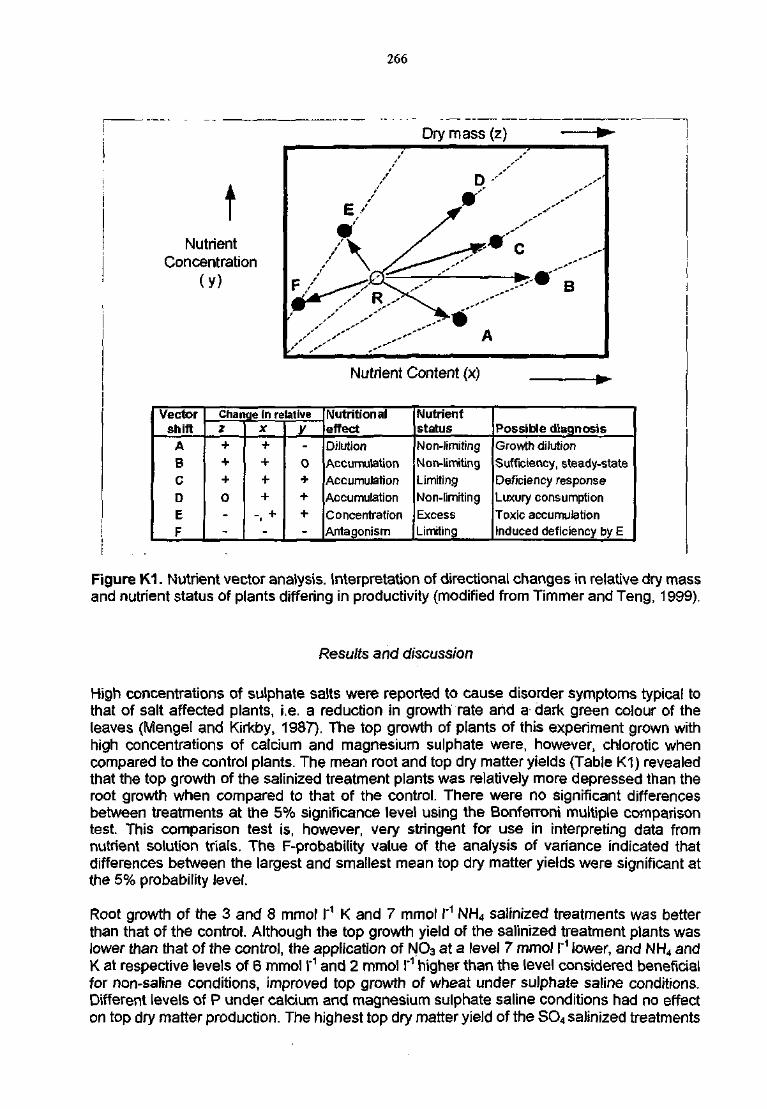
266

tNutrient

Concentration(y)

Nutrient Content (x)

Vectorshift

ABCDEF

Chanqe in relative

z+++0

X

++++

-, +

y

0+++

NutritionaleffectDilutionAccumulationAccumulationAccumulationConcentrationAntagonism

NutrientstatusNon-limitingNon-limitingLimitingNon-limitingExcessLimiting

Possible diagnosisGrowth dilutionSufficiency, steady-stateDeficiency responseLuxury consumptionToxic accumulationInduced deficiency by E

Figure K1. Nutrient vector analysis. Interpretation of directional changes in relative dry massand nutrient status of plants differing in productivity (modified from Timmer and Teng, 1999).

Results and discussion

High concentrations of sulphate salts were reported to cause disorder symptoms typical tothat of salt affected plants, i.e. a reduction in growth rate arid a dark green colour of theleaves (Mengef and Kirkby, 1987). The top growth of plants of this experiment grown withhigh concentrations of calcium and magnesium sulphate were, however, chlorotic whencompared to the control plants. The mean root and top dry matter yields (Table K1) revealedthat the top growth of the salinized treatment plants was relatively more depressed than theroot growth when compared to that of the control. There were no significant differencesbetween treatments at the 5% significance level using the Bonferroni multiple comparisontest. This comparison test is, however, very stringent for use in interpreting data fromnutrient solution trials. The F-probability value of the analysis of variance indicated thatdifferences between the largest and smallest mean top dry matter yields were significant atthe 5% probability level.

Root growth of the 3 and 8 mmol I"1 K and 7 mmol I"1 NH4 salinized treatments was betterthan that of the control. Although the top growth yield of the salinized treatment plants waslower than that of the control, the application of NO3 at a level 7 mmol I"1 lower, and NH4 andK at respective levels of 6 mmol I'1 and 2 mmol I'1 higher than the level considered beneficialfor non-saline conditions, improved top growth of wheat under sulphate saline conditions.Different levels of P under calcium and magnesium sulphate saline conditions had no effecton top dry matter production. The highest top dry matter yield of the SO4 salinized treatments

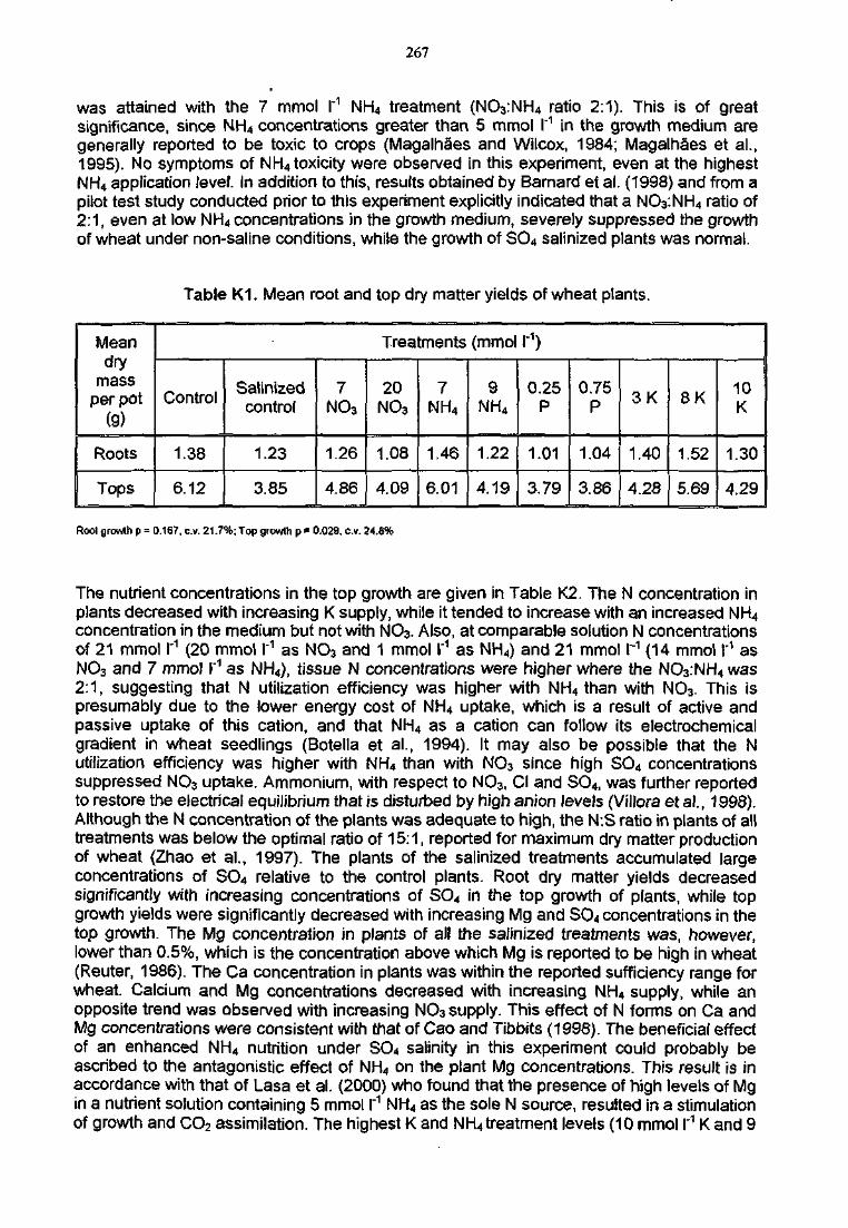
267

was attained with the 7 mmol I"1 NH4 treatment (NO3:NH4 ratio 2:1). This is of greatsignificance, since NH4 concentrations greater than 5 mmol I'1 in the growth medium aregenerally reported to be toxic to crops (Magalhaes and Wilcox, 1984; Magalhaes et al.,1995). No symptoms of NH4toxicity were observed in this experiment, even at the highestNH4 application level. In addition to this, results obtained by Barnard et al. (1998) and from apilot test study conducted prior to this experiment explicitly indicated that a NO^NHU ratio of2:1, even at low NH4 concentrations in the growth medium, severely suppressed the growthof wheat under non-saline conditions, while the growth of SO4 salinized plants was normal.

Table K1. Mean root and top dry matter yields of wheat plants.

Meandry

massper pot

(g)

Roots

Tops

Treatments (mmol I"1)

Control

1.38

6.12

Salinizedcontrol

1.23

3.85

7NO3

1.26

4.86

20NO3

1.08

4.09

7NH4

1.46

6.01

9NH4

1.22

4.19

0.25P

1.01

3.79

0.75P

1.04

3.86

3 K

1.40

4.28

8 K

1.52

5.69

10K

1.30

4.29

Root growth p = 0.167, c.v. 21.7%; Top growth p = 0.029, c.v. 24.8%

The nutrient concentrations in the top growth are given in Table K2. The N concentration inplants decreased with increasing K supply, while it tended to increase with an increased NH4

concentration in the medium but not with NO3. Also, at comparable solution N concentrationsof 21 mmol I'1 (20 mmol I"1 as NO3 and 1 mmol I"1 as NH4) and 21 mmol r1 (14 mmol I'1 asNO3 and 7 mmoJ I"1 as NH4), tissue N concentrations were higher where the NO3.NH4 was2:1, suggesting that N utilization efficiency was higher with NH4 than with NO3. This ispresumably due to the lower energy cost of NH4 uptake, which is a result of active andpassive uptake of this cation, and that NH4 as a cation can follow its electrochemicalgradient in wheat seedlings (Botella et al., 1994). It may also be possible that the Nutilization efficiency was higher with NH4 than with NO3 since high SO4 concentrationssuppressed NO3 uptake. Ammonium, with respect to NO3, Cl and SO4, was further reportedto restore the electrical equilibrium that is disturbed by high anion levels (Villora et al., 1998).Although the N concentration of the plants was adequate to high, the N:S ratio in plants of alltreatments was below the optimal ratio of 15:1, reported for maximum dry matter productionof wheat (Zhao et al., 1997). The plants of the salinized treatments accumulated largeconcentrations of SO4 relative to the control plants. Root dry matter yields decreasedsignificantly with increasing concentrations of SO4 in the top growth of plants, while topgrowth yields were significantly decreased with increasing Mg and SO4 concentrations in thetop growth. The Mg concentration in plants of all the salinized treatments was, however,lower than 0.5%, which is the concentration above which Mg is reported to be high in wheat(Reuter, 1986), The Ca concentration in plants was within the reported sufficiency range forwheat. Calcium and Mg concentrations decreased with increasing NH4 supply, while anopposite trend was observed with increasing NO3 supply. This effect of N forms on Ca andMg concentrations were consistent with that of Cao and Tibbits (1998). The beneficial effectof an enhanced NH4 nutrition under SO4 salinity in this experiment could probably beascribed to the antagonistic effect of NH4 on the plant Mg concentrations. This result is inaccordance with that of Lasa et al. (2000) who found that the presence of high levels of Mgin a nutrient solution containing 5 mmol I'1 NH4 as the sole N source, resulted in a stimulationof growth and CO2 assimilation. The highest K and NH4 treatment levels (10 mmol I"1 K and 9

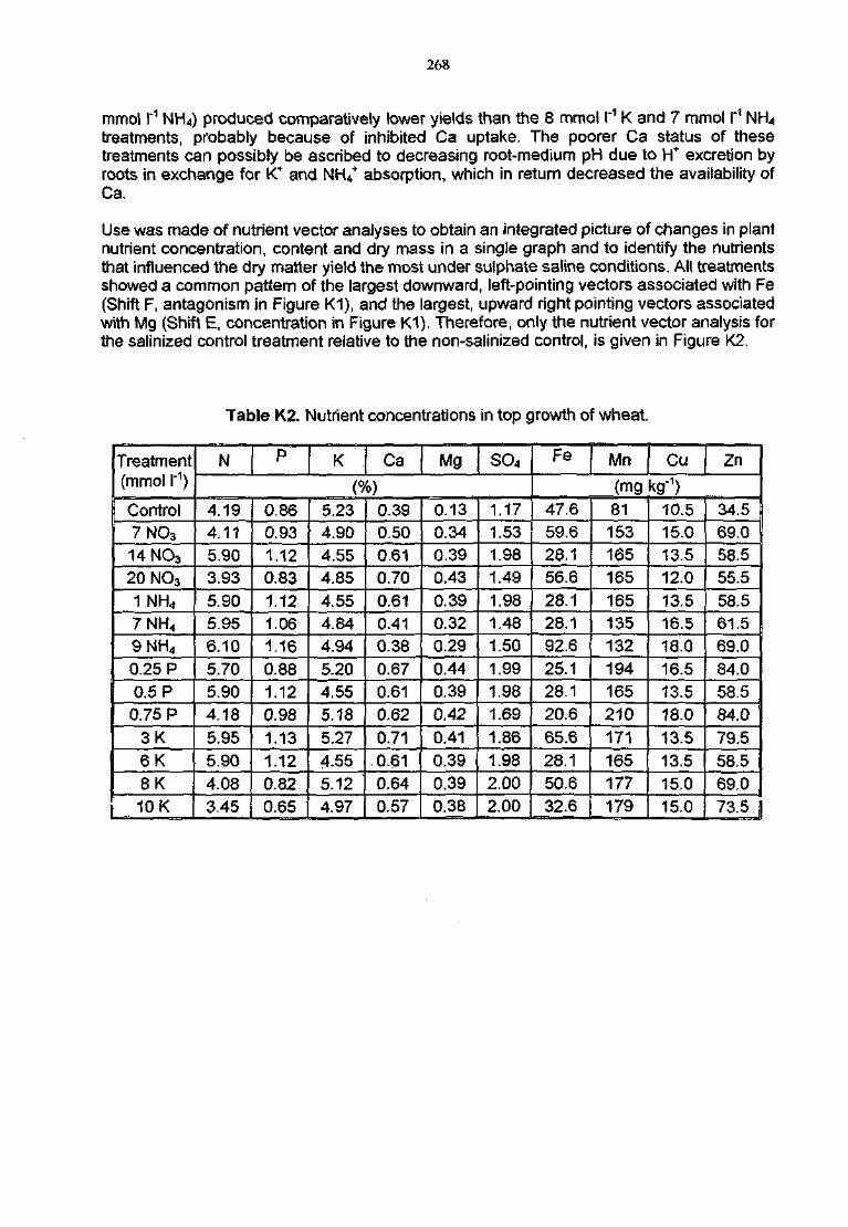
268

mmol I"1 NH4) produced comparatively lower yields than the 8 mmol I"1 K and 7 mmol I"1

treatments, probably because of inhibited Ca uptake. The poorer Ca status of thesetreatments can possibly be ascribed to decreasing root-medium pH due to H+ excretion byroots in exchange for K+ and NH4

+ absorption, which in return decreased the availability ofCa.

Use was made of nutrient vector analyses to obtain an integrated picture of changes in plantnutrient concentration, content and dry mass in a single graph and to identify the nutrientsthat influenced the dry matter yield the most under sulphate saline conditions. All treatmentsshowed a common pattern of the largest downward, left-pointing vectors associated with Fe(Shift F, antagonism in Figure K1), and the largest, upward right pointing vectors associatedwith Mg (Shift E, concentration in Figure K1). Therefore, only the nutrient vector analysis forthe salinized control treatment relative to the non-salinized control, is given in Figure K2.

Table K2. Nutrient concentrations in top growth of wheat.

Treatment(mmol I"1)

Control7NO3

14NO3

20NO3

1 NH4

7NH<9NH<0.25 P0.5 P0.75 P

3K6 K8K10 K

N P K : Ca Mg SO4

(%)4.194.115.903.935.905.956.105.705.904.185.955.904.083.45

0.860.931.120.831.121.061.160.881.120.981.131.120.820.65

5.234.904.554.854.554.844.945.204.555.185.274.555.124.97

0.390.500.610.700.610.410.380.670.610.620.710.610.640.57

0.130.340.390.430.390.320.290.440.390,420,410.390.390.38

1.171.531.981.491.981.481.501.991.981.691.861.982.002.00

Fe Mn Cu Zn

<mg kg"1)47.659.628.156.628.128.192.625.128.120.665.628.150.632.6

81153165165165135132194165210171165177179

10.515.013.512.013.516.518.016.513.518.013.513.515.015.0

34.569.058.555.558.561.569.084.058.584.079.558.569.073.5 I

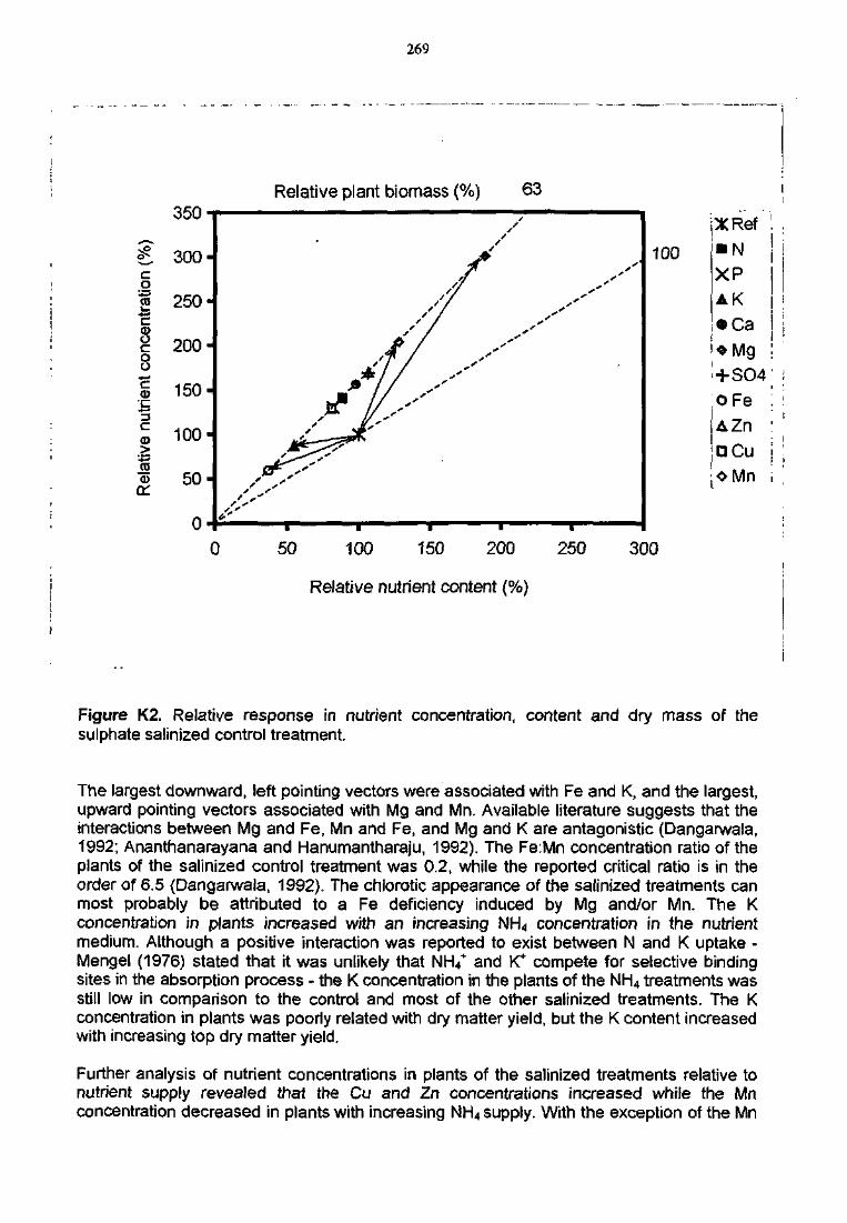
269

Relative plant biomass (%) 63350

co

8§

C

>

19

a:

100

I

jXRef ; .• N I iXPAK©Ca

0 50 100 150 200 250 300

Relative nutrient content (%)

+SO4 ;oFe !AZnncu | :

Figure K2. Relative response in nutrient concentration, content and dry mass of thesulphate salinized control treatment.

The largest downward, left pointing vectors were associated with Fe and K, and the largest,upward pointing vectors associated with Mg and Mn. Available literature suggests that theinteractions between Mg and Fe, Mn and Fe, and Mg and K are antagonistic (Dangarwala,1992; Ananthanarayana and Hanumantharaju, 1992). The Fe:Mn concentration ratio of theplants of the salinized control treatment was 0.2, while the reported critical ratio is in theorder of 6.5 (Dangarwala, 1992). The chlorotic appearance of the salinized treatments canmost probably be attributed to a Fe deficiency induced by Mg and/or Mn. The Kconcentration in plants increased with an increasing NH* concentration in the nutrientmedium. Although a positive interaction was reported to exist between N and K uptake -Mengel (1976) stated that it was unlikely that NH4

+ and K+ compete for selective bindingsites in the absorption process - the K concentration in the plants of the NH4 treatments wasstill low in comparison to the control and most of the other salinized treatments. The Kconcentration in plants was poorly related with dry matter yield, but the K content increasedwith increasing top dry matter yield.

Further analysis of nutrient concentrations in plants of the salinized treatments relative tonutrient supply revealed that the Cu and Zn concentrations increased while the Mnconcentration decreased in plants with increasing NH4 supply. With the exception of the Mn

270

concentration in plants of the control treatment, the plants of the 7 and 9 mmol I'1 NH4

treatments had the lowest Mn status. The Mn concentration in plants further significantlyincreased with increasing plant Mg concentration. In contradiction to this, several reportshave shown that the Mn concentration in plants was decreased with an increasing Mg supplyand concentration in plants (Mengel and Kirkby, 1987; Huang and Redmann, 1995). The Pconcentration in plants decreased with an increasing K supply and was the lowest for the 10mmol I"1 K treatment. This value was, however, still higher than the upper critical literaturenorm.

Conclusions

High concentrations of calcium and magnesium sulphate in the nutrient solution suppressedgrowth of wheat plants. Decreases in yield were associated with significant increases inplant concentrations of SO4 and Mg. Nutrient vector analysis revealed that highconcentrations of calcium and magnesium sulphate in the growth medium decreased Fe andK uptake, while increasing Mg and Mn uptake the most.

The application of NO3 at a level 7 mmol r1 lower, and IMH4 and K at respective levels of 6mmol I"1 and 2 mmol I"1 higher than the level considered beneficial for non-saline conditions,improved top growth of wheat under sulphate saline conditions.

The unexpected beneficial effect of an enhanced NH4 nutrition under SO4 salinity canprobably be ascribed to the antagonistic effect of NH4 on the plant Mg and Mnconcentrations and/or to NH4 being a supplementary N source when large SO4

concentrations suppressed NO3 uptake, since N utilization efficiency was higher with NH4

than with NO3 at similar solution concentrations. !n practice this could mean that theinclusion of NH4-fertilizers in a NO3:NH4 ratio of 2:1, could be advantageous when irrigatingwheat with water containing high levels of Ca and Mg sulphate. Care should, however, beexercised that large application levels of NH^fertilizers does not suppress Ca uptake byplants.

The results obtained from the solution culture trial must be interpreted with caution, since theeffect of sulphate salinity on nutrient availability and uptake may differ in the field, particularlyfor P and K, since their concentrations are controlled by the solid phase and are difficult tomeasure or predict. Confirmation of the results obtained should thus be sought in field trials.

APPENDIX L

Herbicide effects

272

Introduction

Herbicides are widely used to control weeds in crop production, particularly in large-scalefarming. They are the most practical way of coping with weeds at this level of farming, andprobably at all levels of crop production (Akobundu, 1987, Ashton and Crafts, 1981,Ktingman etal., 1982). The behaviour of herbicides in the soil and in the plant is influencedby soil factors, type of herbicide, environmental factors and plant species. The combinedeffect of these factors will determine the fate of a herbicide in the environment (Walker,1994; Akobundu, 1987; Weaver and Reinhardt, 1998). Of particular importance is howpotential interactions could influence the following important criteria for herbicideperformance: weed control efficacy, the tolerance of crop species, and the potential forherbicides to leach to groundwater.

The soil solution characteristics, in addition to pH and soil colloids, govern to a large extentherbicide behaviour (Walker, 1994). Clay et al. (1995) reported the effects of fertilizerapplication on herbicide activity or efficacy. Application of ammonia fertilizer to the soilincreased soil pH and dissolved organic carbon. This reduced atrazine adsorption andresulted in increased atrazine in the soil solution. The principle behind this is that someherbicides compete with charged electrolytes for adsorption sites on the soil colloids. Thereplacing power of cations on clay and humus generally follows the order C+ < C2+ < C3+

(Brady, 1974). The divalent ions are more competitive and more strongly adsorbed thanmonovalent ions.

Stmazine and atrazine adsorption was reportedly influenced by high electrolyteconcentrations. Hurle and Freed (1972) ascribed stronger herbicide adsorption in thepresence of high levels of electrolytes to depressed herbicide solubility. Dao and Lavy(1978) reported that atrazine adsorption increased as KCI and NH4CI concentrationsincreased in the soil solution. Clay et al. (1995) found interaction between ammonia andatrazine. Ammonia-based fertilizers increase pH, and at high pH, atrazine sorption isdecreased. This results in high atrazine in the soil solution, thus increasing the possibility ofatrazine leaching, as well as the risk to sensitive follow-up crops. Changes in soil pHinfluence the behaviour of herbicides. Chemical hydrolysis is pH-dependent for mostherbicides. The atrazine molecule is stable under neutral pH conditions, but rapid chemicalhydrolysis occurs under highly acid or alkaline conditions (Armstrong et al., 1967).

Herbicide interaction with mine water is very possible due to the high concentration ofelectrolytes in this water. The quality of water used as a solvent in herbicide application isknown to influence the efficacy of certain herbicides. This kind of interaction could lead to:

• Increased herbicide leaching with the end result of groundwater contamination andpoor weed control due to reduced herbicide activity in the root-zone,

• Increased herbicide concentration in the soil solution which may result in crop injuryand reduced selectivity,

• Stronger adsorption of herbicides on soil colloids, resulting in inadequate weedcontrol, and increased persistence which could promote environmental pollutionand/or cause damage to follow-up crops.

Objectives

The objectives of this preliminary investigation were to determine the influence of mine wateron the three important performance criteria for herbicides, namely:

• Weed control efficacy;

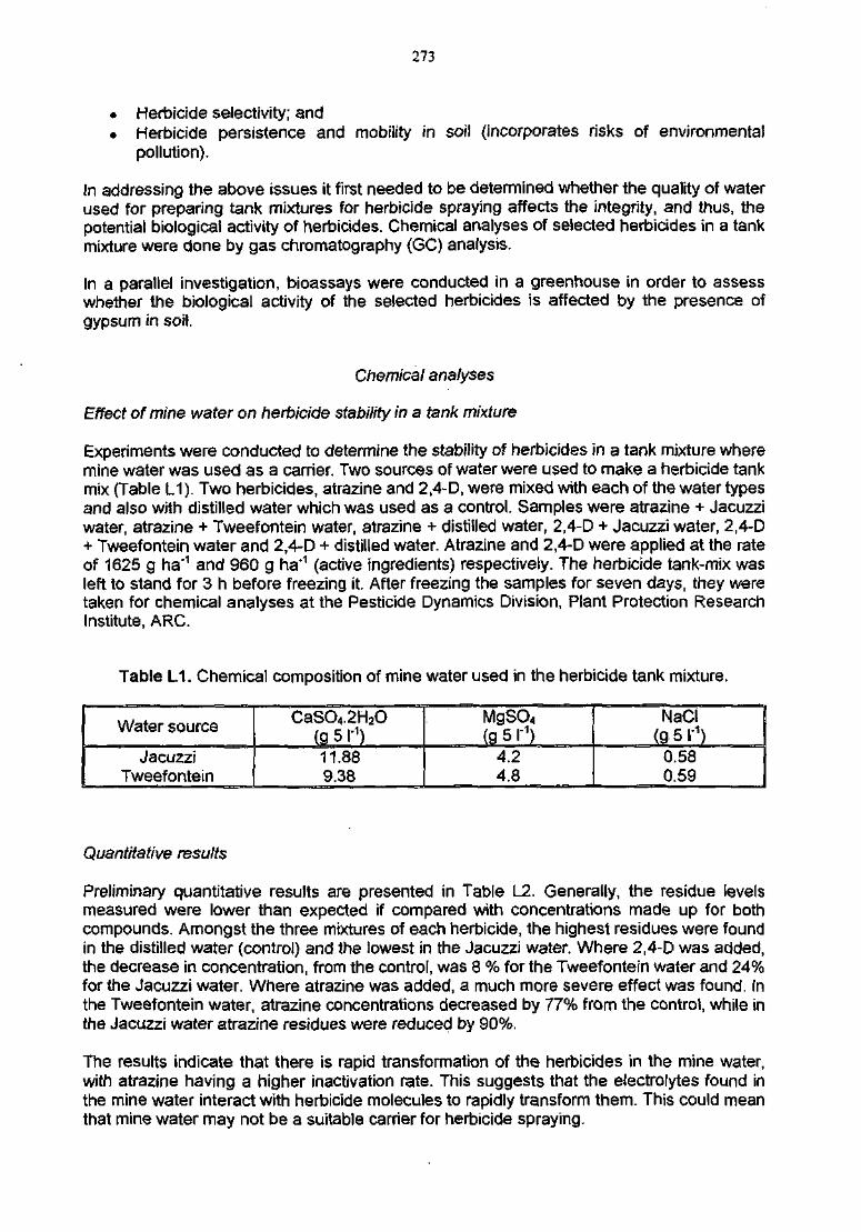
273

• Herbicide selectivity; and• Herbicide persistence and mobility in soil (incorporates risks of environmental

pollution).

In addressing the above issues it first needed to be determined whether the quality of waterused for preparing tank mixtures for herbicide spraying affects the integrity, and thus, thepotential biological activity of herbicides. Chemical analyses of selected herbicides in a tankmixture were done by gas chromatography (GC) analysis.

In a parallel investigation, bioassays were conducted in a greenhouse in order to assesswhether the biological activity of the selected herbicides is affected by the presence ofgypsum in soil.

Chemical analyses

Effect of mine water on herbicide stability in a tank mixture

Experiments were conducted to determine the stability of herbicides in a tank mixture wheremine water was used as a carrier. Two sources of water were used to make a herbicide tankmix (Table L1). Two herbicides, atrazine and 2,4-D, were mixed with each of the water typesand also with distilled water which was used as a control. Samples were atrazine + Jacuzziwater, atrazine + Tweefontein water, atrazine + distilled water, 2,4-D + Jacuzzi water, 2,4-D+ Tweefontein water and 2,4-D + distilled water. Atrazine and 2,4-D were applied at the rateof 1625 g ha"1 and 960 g ha*1 (active ingredients) respectively. The herbicide tank-mix wasleft to stand for 3 h before freezing it. After freezing the samples for seven days, they weretaken for chemical analyses at the Pesticide Dynamics Division, Plant Protection ResearchInstitute, ARC.

Table L1. Chemical composition of mine water used in the herbicide tank mixture.

Water source

JacuzziTweefontein

CaSO4.2H2O(g 5 r1)11.889.38

MgSCU(g 51-1)

4.24.8

NaCI(gsr1)

0.580.59

Quantitative results

Preliminary quantitative results are presented in Table 12. Generally, the residue levelsmeasured were lower than expected if compared with concentrations made up for bothcompounds. Amongst the three mixtures of each herbicide, the highest residues were foundin the distilled water (control) and the lowest in the Jacuzzi water. Where 2,4-D was added,the decrease in concentration, from the control, was 8 % for the Tweefontein water and 24%for the Jacuzzi water. Where atrazine was added, a much more severe effect was found. Inthe Tweefontein water, atrazine concentrations decreased by 77% from the control, while inthe Jacuzzi water atrazine residues were reduced by 90%.

The results indicate that there is rapid transformation of the herbicides in the mine water,with atrazine having a higher inactivation rate. This suggests that the electrolytes found inthe mine water interact with herbicide molecules to rapidly transform them. This could meanthat mine water may not be a suitable carrier for herbicide spraying.

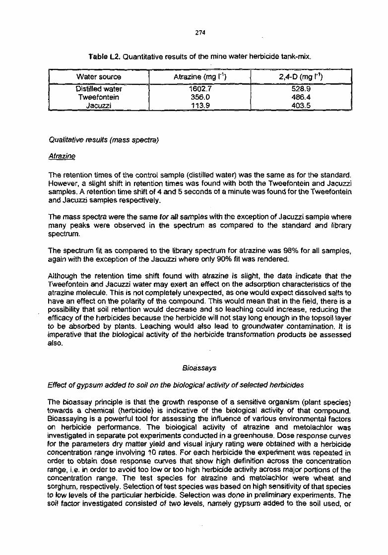
274

Table L2. Quantitative results of the mine water herbicide tank-mix.

Water source

Distilled waterTweefontern

Jacuzzi

Atrazine (mg I"1)

1602.7356.0113.9

2,4-D (mg f1)

528.9486.4403.5

Qualitative results (mass spectra)

Atrazine

The retention times of the control sample (distilled water) was the same as for the standard.However, a slight shift in retention times was found with both the Tweefontein and Jacuzzisamples. A retention time shift of 4 and 5 seconds of a minute was found for the Tweefonteinand Jacuzzi samples respectively.

The mass spectra were the same for all samples with the exception of Jacuzzi sample wheremany peaks were observed in the spectrum as compared to the standard and libraryspectrum.

The spectrum fit as compared to the library spectrum for atrazine was 98% for all samples,again with the exception of the Jacuzzi where only 90% fit was rendered.

Although the retention time shift found with atrazine is slight, the data indicate that theTweefontein and Jacuzzi water may exert an effect on the adsorption characteristics of theatrazine molecule. This is not completely unexpected, as one would expect dissolved salts tohave an effect on the polarity of the compound. This would mean that in the field, there is apossibility that soil retention would decrease and so leaching could increase, reducing theefficacy of the herbicides because the herbicide will not stay long enough in the topsoil layerto be absorbed by plants. Leaching would also lead to groundwater contamination. It isimperative that the biological activity of the herbicide transformation products be assessedalso.

Bioassays

Effect of gypsum added to soil on the biological activity of selected herbicides

The bioassay principle is that the growth response of a sensitive organism (plant species)towards a chemical (herbicide) is indicative of the biological activity of that compound.Bioassaying is a powerful tool for assessing the influence of various environmental factorson herbicide performance. The biological activity of atrazine and metolachlor wasinvestigated in separate pot experiments conducted in a greenhouse. Dose response curvesfor the parameters dry matter yield and visual injury rating were obtained with a herbicideconcentration range involving 10 rates. For each herbicide the experiment was repeated inorder to obtain dose response curves that show high definition across the concentrationrange, i.e. in order to avoid too low or too high herbicide activity across major portions of theconcentration range. The test species for atrazine and metolachlor were wheat andsorghum, respectively. Selection of test species was based on high sensitivity of that speciesto low levels of the particular herbicide. Selection was done in preliminary experiments. Thesoil factor investigated consisted of two levels, namely gypsum added to the soil used, or

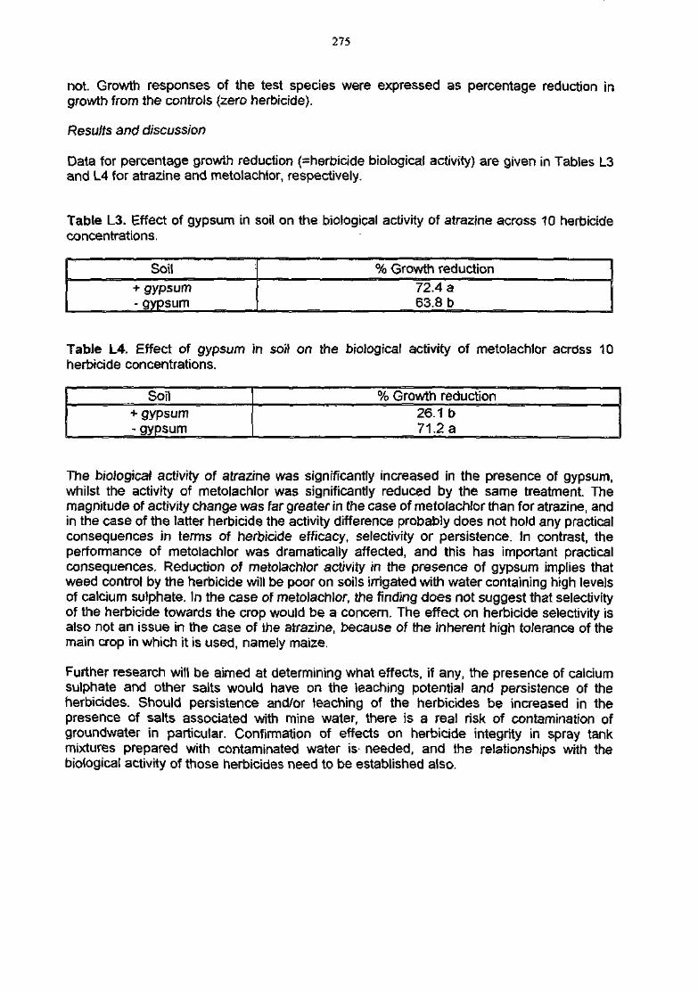
275

not. Growth responses of the test species were expressed as percentage reduction ingrowth from the controls (zero herbicide).

Results and discussion

Data for percentage growth reduction (=herbicide biological activity) are given in Tables L3and L4 for atrazine and metolachlor, respectively.

Table L3. Effect of gypsum in soil on the biological activity of atrazine across 10 herbicideconcentrations.

Soil+ gypsum- gypsum

% Growth reduction72.4 a63.8 b

Table L4. Effect of gypsum in soil on the biological activity of metofachlor acrdss 10herbicide concentrations.

Soil+ gypsum- gypsum

% Growth reduction26.1 b71.2 a

The biological activity of atrazine was significantly increased in the presence of gypsum,whilst the activity of metolachlor was significantly reduced by the same treatment. Themagnitude of activity change was far greater in the case of metolachlor than for atrazine, andin the case of the latter herbicide the activity difference probably does not hold any practicalconsequences in terms of herbicide efficacy, selectivity or persistence. In contrast, theperformance of metolachlor was dramatically affected, and this has important practicalconsequences. Reduction of metolachlor activity in the presence of gypsum implies thatweed control by the herbicide will be poor on soils irrigated with water containing high levelsof calcium sulphate. In the case of metolachlor, the finding does not suggest that selectivityof the herbicide towards the crop would be a concern. The effect on herbicide selectivity isalso not an issue in the case of the atrazine, because of the inherent high tolerance of themain crop in which it is used, namely maize.

Further research will be aimed at determining what effects, if any, the presence of calciumsulphate and other salts would have on the leaching potential and persistence of theherbicides. Should persistence and/or leaching of the herbicides be increased in thepresence of salts associated with mine water, there is a real risk of contamination ofgroundwater in particular. Confirmation of effects on herbicide integrity in spray tankmixtures prepared with contaminated water is needed, and the relationships with thebiological activity of those herbicides need to be established also.

APPENDIX M

Theory of the finite-difference water balance andconvection/dispersion solute redistribution used in

the SWB model

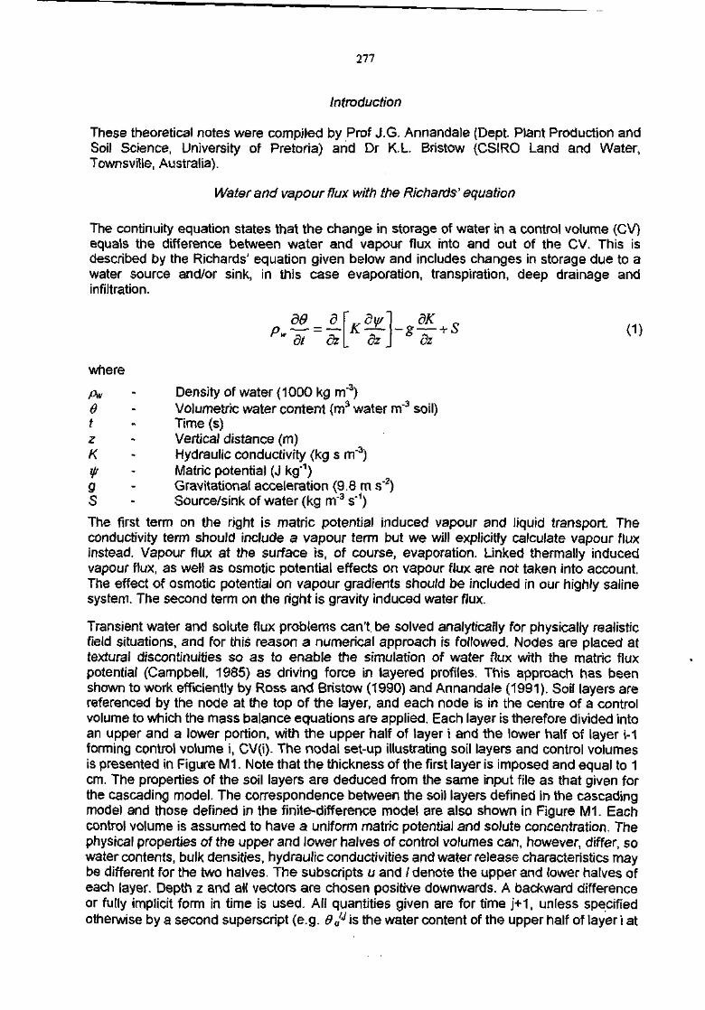
277

Introduction

These theoretical notes were compiled by Prof J.G. Annandale (Dept. Plant Production andSoil Science, University of Pretoria) and Dr K.L. Bristow (CS1R0 Land and Water,Townsville, Australia).

Water and vapour flux with the Richards' equation

The continuity equation states that the change in storage of water in a control volume (CV)equals the difference between water and vapour flux into and out of the CV. This isdescribed by the Richards' equation given below and includes changes in storage due to awater source and/or sink, in this case evaporation, transpiration, deep drainage andinfiltration.

dt dz dz ° dz(1)

where

pw - Density of water (1000 kg m'3)0 - Volumetric water content (m3 water m"3 soil)t - Time (s)z - Vertical distance (m)K - Hydraulic conductivity (kg s m"3)f - Matric potential (J kg'1)g - Gravitational acceleration (9.8 m s'2)S - Source/sink of water (kg m'3 s'1)

The first term on the right is matric potential induced vapour and liquid transport. Theconductivity term should include a vapour term but we will explicitly calculate vapour fluxinstead. Vapour flux at the surface is, of course, evaporation. Linked thermally inducedvapour flux, as welt as osmotic potential effects on vapour flux are not taken into account.The effect of osmotic potential on vapour gradients should be included in our highly salinesystem. The second term on the right is gravity induced water flux.

Transient water and solute flux problems can't be solved analytically for physically realisticfield situations, and for this reason a numerical approach is followed. Nodes are placed attextural discontinuities so as to enable the simulation of water flux with the matric fluxpotential (Campbell, 1985) as driving force in layered profiles. This approach has beenshown to work efficiently by Ross and Bristow (1990) and Annandale (1991). Soil layers arereferenced by the node at the top of the layer, and each node is in the centre of a controlvolume to which the mass balance equations are applied. Each layer is therefore divided intoan upper and a lower portion, with the upper half of layer i and the lower half of layer i-1forming control volume i, CV(i). The nodal set-up illustrating soil layers and control volumesis presented in Figure M l . Note that the thickness of the first layer is imposed and equal to 1cm. The properties of the soil layers are deduced from the same input file as that given forthe cascading model. The correspondence between the soil layers defined in the cascadingmodel and those defined in the finite-difference model are also shown in Figure M1. Eachcontroi volume is assumed to have a uniform matric potential and solute concentration. Thephysical properties of the upper and lower halves of control volumes can, however, differ, sowater contents, bulk densities, hydraulic conductivities and water release characteristics maybe different for the two halves. The subscripts u and / denote the upper and lower halves ofeach layer. Depth z and all vectors are chosen positive downwards. A backward differenceor fully implicit form in time is used. AH quantities given are for time j+1, unless specifiedotherwise by a second superscript (e.g. ffu'

J is the water content of the upper half of layer i at

278

time jSf). A description of the functions used to describe the hydraulic properties is firstgiven, followed by the discretized version of the terms in the Richards' equation.

Hydraulic properties

It is essential that the model be able to estimate matric potential from water content and viceversa, i.e. a water retention function is required. Functions available in the literature includethe unsmoothed Brooks-Corey function (Brooks and Corey, 1964, 1966), which reduces tothe Campbell functions (Campbell, 1974, 1985) if the residual water content is taken as zero,the smoothed Brooks-Corey function (Hutson and Cass, 1987) and the van Genuchten(1980) function.

The smoothed Brooks-Corey function is used in this model. It is given by:

6 = 6s

T ,„ ^ , , , in\

), y/i < v < 0 (3)

6 = 0S, 0<W (4)

with ij/e the air entry potential (J kg'1), b the slope of a log-log water retention function, # athreshold water potential, where

\j/i = if/ e a (5)

a = 2£)/(1+2ib) (6)

The derivatives needed for the Newton-Raphson solution (as discussed later) are

d& ~°T" = T~' Vs^' (8)dy/ by/

dy/

~ = 0, 0<y/ (10)dy/

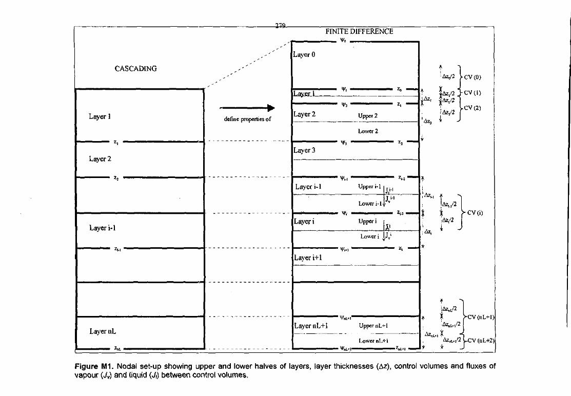
CASCADING

Layer 1

Layer 2

Layer i-1

Zi-I

Layer nL

27g

define properties of

FINITE DIFFERENCE%

Layer 0

v.La^eiJ111 % •

Z,

z,

Layer 2 Upper 2

Lower 2

Layer 3

Zi-I1

Layer i-1 Upper M

Layer i

Lower i-1 y *

Upper i

Lower i

Layer i+1

HV+i"

Layer nL+1 Upper nL+1

Lower nL+1

Az,

X ?-cv(i)iAz/2

4

CV(nL+l

AznLt/2Lcv(nL+2J

Figure M1. Nodal set-up showing upper and lower halves of layers, layer thicknesses (Az), control volumes and fluxes ofvapour (Jv) and liquid (Jf) between control volumes.

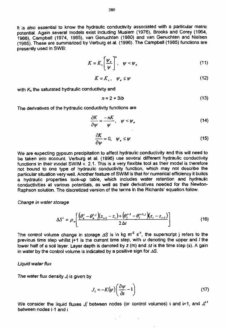
280

!t is also essential to know the hydraulic conductivity associated with a particular matricpotential. Again several models exist including Mualem (1976), Brooks and Corey (1964,1966), Campbell (1974, 1985), van Genuchten (1980) and van Genuchten and Nielsen(1985). These are summarized by Verburg et al. (1996). The Campbell (1985) functions arepresently used in SWB:

r ~iM

¥<Ve C1)

K=KS, We<y (12)

with Ks the saturated hydraulic conductivity and

n = 2 + 3/b (13)

The derivatives of the hydraulic conductivity functions are

8K ~"K V<V. (14)

= 0, y/ <y/ (15)dy/

We are expecting gypsum precipitation to affect hydraulic conductivity and this will need tobe taken into account. Verburg et al. (1996) use several different hydraulic conductivityfunctions in their model SWIM v, 2.1. This is a very flexible tool as their model is thereforenot bound to one type of hydraulic conductivity function, which may not describe theparticular situation very well. Another feature of SWIM is that for numerical efficiency it buildsa hydraulic properties look-up table, which includes water retention and hydraulicconductivities at various potentials, as well as their derivatives needed for the Newton-Raphson solution. The discretized version of the terms in the Richards' equation follow.

Change in water storage

+1 ' ; V ' '- ^ ^ (16)

2At JThe control volume change in storage AS is in kg m'2 s"1, the superscript j refers to theprevious time step whilst j+1 is the current time step, with u denoting the upper and / thelower half of a soil layer. Layer depth is denoted by z (m) and At is the time step (s). A gainin water by the control volume is indicated by a positive sign for AS.

Liquid water flux

The water flux density J, is given by

• / ,= -* : (y ) [—-1 | (17)

We consider the liquid fluxes j} between nodes (or control volumes) i and t+1, and jfbetween nodes i-1 and i

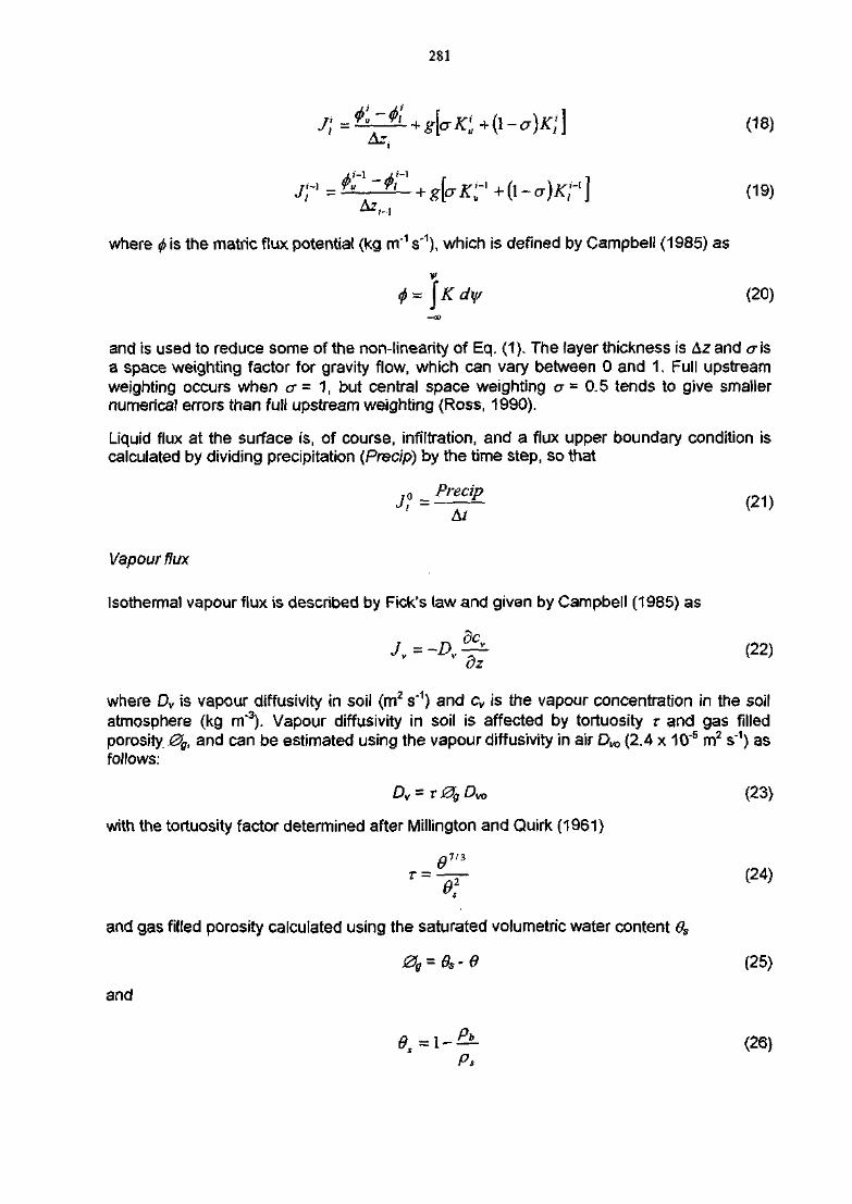
281

g [ i +(\-a)K\\ (18)

(19)

where <f> is the matric flux potential (kg m"1 s'1), which is defined by Campbell (1985) as

(20)

and is used to reduce some of the non-linearity of Eq. (1). The layer thickness is Az and CMSa space weighting factor for gravity flow, which can vary between 0 and 1. Full upstreamweighting occurs when a = 1, but central space weighting a = 0.5 tends to give smallernumerical errors than full upstream weighting (Ross, 1990).

Liquid flux at the surface is, of course, infiltration, and a flux upper boundary condition iscalculated by dividing precipitation (Precip) by the time step, so that

Vapour flux

Isothermal vapour flux is described by Fick's law and given by Campbell (1985) as

J = D ^ (22)

where Dv is vapour diffusivity in soil (m2 s'1) and cv is the vapour concentration in the soilatmosphere (kg m'3). Vapour diffusivity in soil is affected by tortuosity r and gas filledporosity 0g, and can be estimated using the vapour diffusivity in air Dw (2.4 x 10~5 m2 s"1) asfollows:

? T O (23)

with the tortuosity factor determined after Millington and Quirk (1961)

r = V (24)

and gas filled porosity calculated using the saturated volumetric water content 6>s

0g=eS'O (25)

and

0, = 1 - — (26)Ps

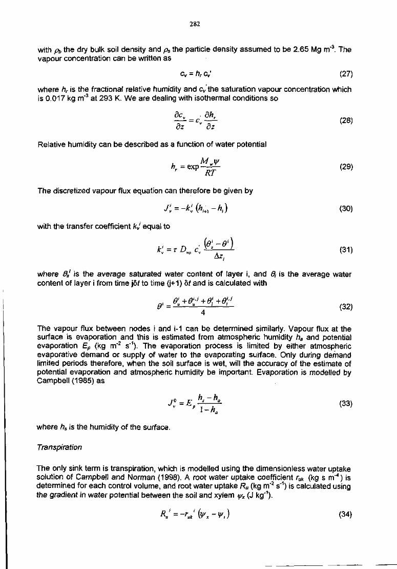
282

with pt> the dry bulk soil density and ps the particle density assumed to be 2.65 Mg m'3. Thevapour concentration can be written as

cv = hr c ; (27)

where hr is the fractional relative humidity and cv the saturation vapour concentration whichis 0.017 kg m'3 at 293 K. We are dealing with isothermal conditions so

d-r=c'-ir <28»d dz

Relative humidity can be described as a function of water potential

^ ^ (29)RT

The discretizecf vapour flux equation can therefore be given by

with the transfer coefficient kj equal to

f JK = z Dvo cv^-~^- (31)

where 8j is the average saturated water content of layer i, and 6{ is the average watercontent of layer i from time jSr to time G+1) & and is calculated with

( 3 2 )

The vapour flux between nodes i and i-1 can be determined similarly. Vapour flux at thesurface is evaporation and this is estimated from atmospheric humidity ha and potentialevaporation Ep (kg m'2 s"1). The evaporation process is limited by either atmosphericevaporative demand or supply of water to the evaporating surface. Only during demandlimited periods therefore, when the soil surface is wet, will the accuracy of the estimate ofpotential evaporation and atmospheric humidity be important. Evaporation is modelled byCampbell (1985) as

J>E*±t <33>where hs is the humidity of the surface.

Transpiration

The only sink term is transpiration, which is modelled using the dimensionless water uptakesolution of Campbell and Norman (1998). A root water uptake coefficient ruk (kg s m4) isdetermined for each control volume, and root water uptake Ru (kg m'2 s"1) is calculated usingthe gradient in water potential between the soil and xylem y/x (J kg'1).

(34)

283

Mass balance

Water needs to be conserved by the model and the mass balance error MBE (kg m"z s"1) isgiven by

MBEj = AS' -J'r +J{ -J'-} +J'V +K (35)

The aim is to find the matric potentials of each control volume that will cause the massbalance error to be negligible, less than some predetermined error limit arbitrarily chosen as1 x 10'7 kg m"2 s"1 or 0.0086 mm d"1 in this model.

Numerical solution

Even though matric flux potential helps linearize the flow equation, this is still non-linear sothe solution method chosen needs to be able to solve non-linear equations. The Newton-Raphson iterative method as described by Campbell (1985) is used, and this involvesdetermining the derivatives of the mass balance equation for CV(i) with respect to thepotentials at nodes i-1, i and i+1 for the present time step. These derivatives form thecoefficient matrix of the solution, which is symmetrical and tri-diagonal. The Thomasalgorithm is then used to find a new set of potentials that better satisfy the condition for massbalance. This simultaneous equation solution procedure is repeated until the acceptedtolerance level is achieved. The derivatives of the components of the mass balance equationfollow.

Storage

dAS' a

2te

p .

'dO[

2 At

dd\1-1(36)

The determination of the differential water capacities 80ldy/ is discussed in the hydraulicproperties section.

Transpiration or root water uptake

iruk (37)

LiQuid fluxes

ay/, = -7^ + gv (38)

( 3 9 )

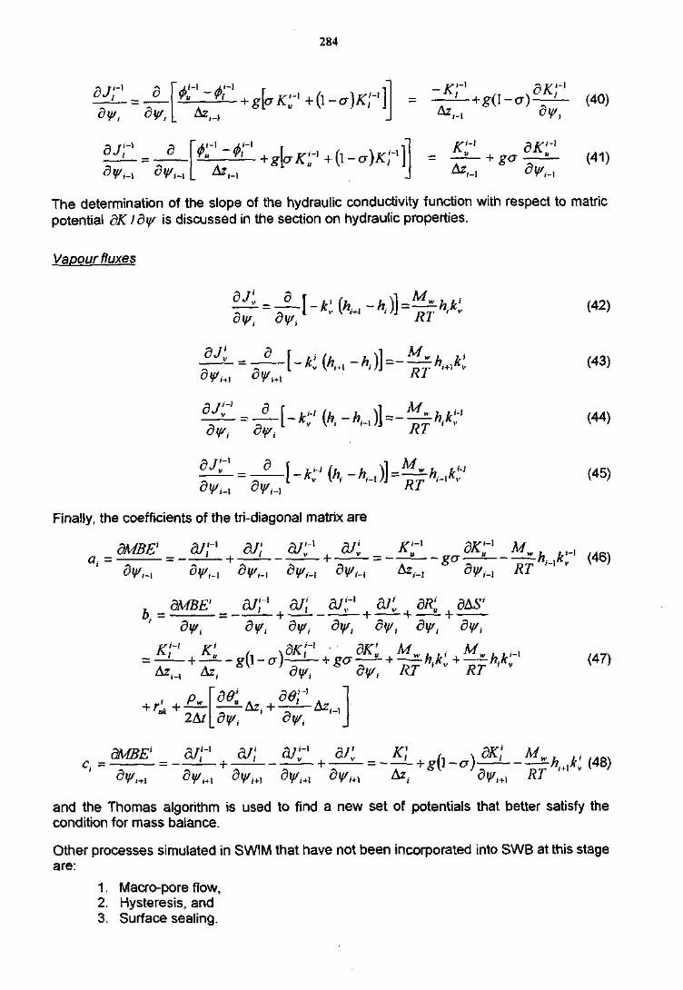
284

ar-1

Az,

i - l

i—i

Az - i

(40)

(41)

The determination of the slope of the hydraulic conductivity function with respect to matricpotential dK Idys is discussed in the section on hydraulic properties.

Vapour fluxes

dJ'v

dy/i

dJjj =

RT(42)

(43)

J-I (44)

dJi; d >i

RT '"

Finally, the coefficients of the tri-diagonal matrix are

= BMBE = a/;' a/; a/;-1 ; a/;

i-i

: i-i Az<

2A^

a/: ^|

a/:: A/.

(45)

(47)

c =! a/;-1 a/;

d „ Az; *K ;dy,M RT

and the Thomas algorithm is used to find a new set of potentials that better satisfy thecondition for mass balance.

Other processes simulated in SWIM that have not been incorporated into SWB at this stageare:

1. Macro-pore flow,2. Hysteresis, and3. Surface sealing.

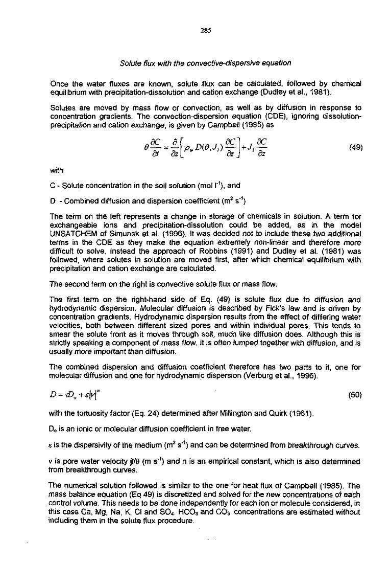
285

Solute flux with the convective-dispersive equation

Once the water fluxes are known, solute flux can be calculated, followed by chemicalequilibrium with precipitation-dissolution and cation exchange (Dudley et al., 1981).

Solutes are moved by mass flow or convection, as well as by diffusion in response toconcentration gradients. The convection-dispersion equation (CDE), ignoring dissolution-precipitation and cation exchange, is given by Campbell (1985) as

dt dz dz(49)

with

C - Solute concentration in the soil solution (mol I"1), and

D - Combined diffusion and dispersion coefficient (m2 s'1)

The term on the left represents a change in storage of chemicals in solution. A term forexchangeable ions and precipitation-dissolution could be added, as in the modelUNSATCHEM of Simunek et al. (1996). It was decided not to include these two additionalterms in the CDE as they make the equation extremely non-linear and therefore moredifficult to solve. Instead the approach of Robbins (1991) and Dudley et al. (1981) wasfollowed, where solutes in solution are moved first, after which chemical equilibrium withprecipitation and cation exchange are calculated.

The second term on the right is convective solute flux or mass flow.

The first term on the right-hand side of Eq. (49) is solute flux due to diffusion andhydrodynamic dispersion. Molecular diffusion is described by Fick's law and is driven byconcentration gradients. Hydrodynamic dispersion results from the effect of differing watervelocities, both between different sized pores and within individual pores. This tends tosmear the solute front as it moves through soil, much like diffusion does. Although this isstrictly speaking a component of mass flow, it is often lumped together with diffusion, and isusually more important than diffusion.

The combined dispersion and diffusion coefficient therefore has two parts to it, one formolecular diffusion and one for hydrodynamic dispersion (Verburg et al., 1996).

D = zDo+£\v\ (50)

with the tortuosity factor (Eq. 24) determined after Millington and Quirk (1961).

Do is an ionic or molecular diffusion coefficient in free water.

e is the dispersivity of the medium (m2 s'1) and can be determined from breakthrough curves.

v is pore water velocity jl/0 (m s'1) and n is an empirical constant, which is also determinedfrom breakthrough curves.

The numerical solution followed is similar to the one for heat flux of Campbell (1985). Themass balance equation (Eq 49) is discretized and solved for the new concentrations of eachcontrol volume. This needs to be done independently for each ion or molecule considered, inthis case Ca, Wig, Na, K, Cl and SCv HCO3 and CO3 concentrations are estimated withoutincluding them in the solute flux procedure.

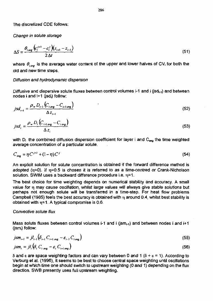
286

The discretized CDE follows:

Change in solute storage

2 At

where 0jflHg, is the average water content of the upper and lower halves of CVj for both the

old and new time steps.

Diffusion and hyctrodynamic dispersion

Diffusive and dispersive solute fluxes between control volumes i-1 and i (jsdM) and betweennodes i and i+1 (jsdj) follow:

jsd. = P">>(C<»"*C"»*) ( 5 3 )

Az,

with Di the combined diffusion dispersion coefficient for layer i and Cavg the time weightedaverage concentration of a particular solute.

C^=tIC'+1+Q-ij)CJ (54)

An explicit solution for solute concentration is obtained if the forward difference method isadopted (rpO). If r|=0.5 is chosen it is referred to as a time-centred or Crank-Nicholsonsolution. SWIM uses a backward difference procedure i.e. ri=1.

The best choice for time weighting depends on numerical stability and accuracy. A smallvalue for r\ may cause oscillation, whilst large values will always give stable solutions butperhaps not enough solute will be transferred in a time-step. For heat flow problemsCampbell (1985) feels the best accuracy is obtained with ri around 0.4, whilst best stability isobtained with r p 1 . A typical compromise is 0.6.

Convective solute flux

Mass sotute fluxes between control volumes i-1 and i (jsmi-i) and between nodes i and i+1follow:

( ) (55)

(56)

5 and e are space weighting factors and can vary between 0 and 1 (8 + E = 1). According toVerburg et al. (1996), it seems to be best to choose central space weighting until oscillationsbegin at which time one should switch to upstream weighting (0 and 1) depending on the fluxdirection. SWB presently uses full upstream weighting.

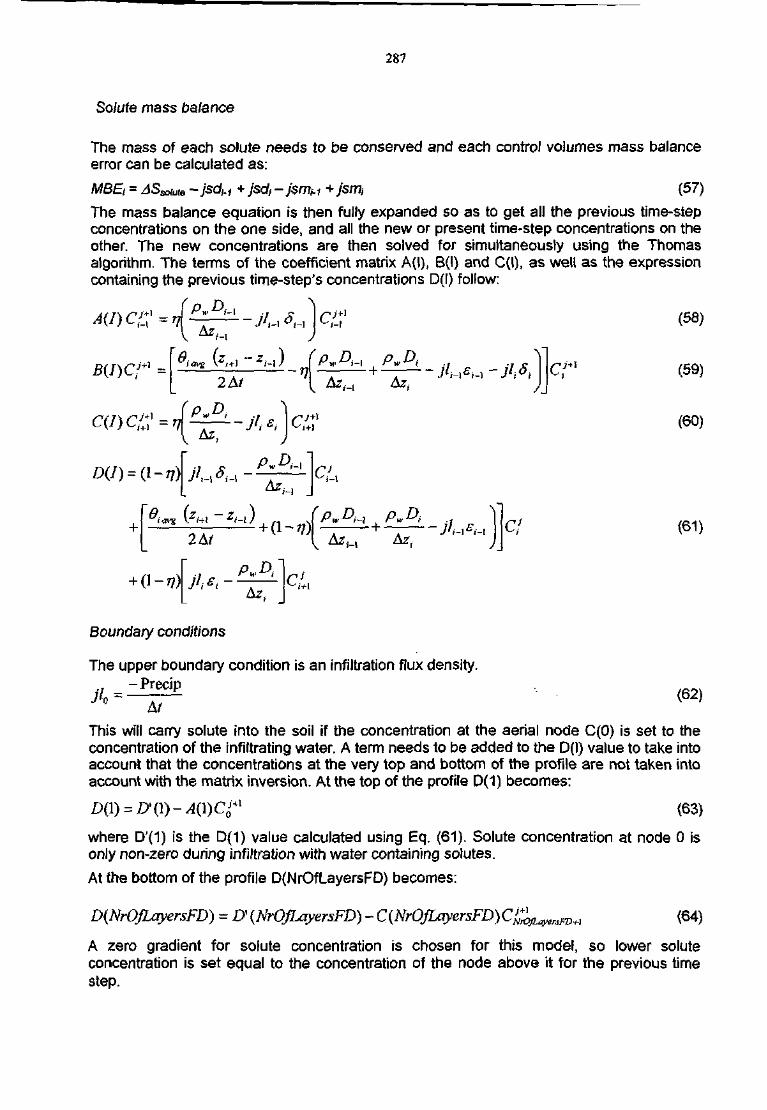
287

Solute mass balance

The mass of each solute needs to be conserved and each control voiumes mass balanceerror can be calculated as:

MBEi = ASsoime -jsdi.i + jsdj-jsm^ + jsm, (57)

The mass balance equation is then fully expanded so as to get all the previous time-stepconcentrations on the one side, and all the new or present time-step concentrations on theother. The new concentrations are then solved for simultaneously using the Thomasalgorithm. The terms of the coefficient matrix A(l), B(l) and C(l), as well as the expressioncontaining the previous time-step's concentrations D(I) follow:

CJ+l

(58)

(59)

(60)

2 At Az.._, Az,Cf (61)

Az,C

Boundary conditions

The upper boundary condition is an infiltration flux density._ -Precip

3 ^(62)

This will carry solute into the soil if the concentration at the aerial node C(0) is set to theconcentration of the infiltrating water. A term needs to be added to the D(l) value to take intoaccount that the concentrations at the very top and bottom of the profile are not taken intoaccount with the matrix inversion. At the top of the profile D(1) becomes:

D(l) = H (1) - A{\) C0J+l (63)

where D'(1) is the D(1) value calculated using Eq. (61). Solute concentration at node 0 isonly non-zero during infiltration with water containing solutes.

At the bottom of the profile D(NrOfLayersFD) becomes:

D{NrOfLayersFD) - £>' {NrOJLayersFD) - C{NrOfLayersFD)C{£NtOJLayersFD+i (64)

A zero gradient for solute concentration is chosen for this model, so lower soluteconcentration is set equal to the concentration of the node above it for the previous timestep.

APPENDIX N

Model validation

289

In this Appendix, additional validation data for the SWB model are presented for wheatgrown during the winter 1999 season at pivot Fourth and for different irrigation treatments(Appendix A, Table A8, replication 2).

Soil water balance and crop growth simulations are shown in Figures N1 to N4 (fieldcapacity and deficit irrigation treatments). Model predictions were reasonable compared tofield measurements.

Simulations of soil water redistribution compared generally well to data measured with heatdissipation sensors for different irrigation treatments and soil depths. The comparisons areshown in Figures N5 to N10. It is not clear why the sensors dried out in the field capacitytreatment in the middle of the season, especially the sensor installed at 26 cm soil depth(Figure N6), as this was not the case for the leaching fraction (Figure N5) and deficitirrigation treatment (Figure N7). This resulted in very low (negative) readings of soil matricpotential. Possible causes are incorrect placement of the sensors, which caused loss ofcontact between the soil and the ceramic matrix of the sensors as the soil was drying, orunusually high root density and water uptake at the site where the sensors were installed.

The model also gave good predictions of the redistribution of single ionic species in the soilprofile. Examples are shown for the major ionic species in irrigation water (calcium,magnesium and sulphate) and the leaching fraction treatment in Figures N11 to N13.

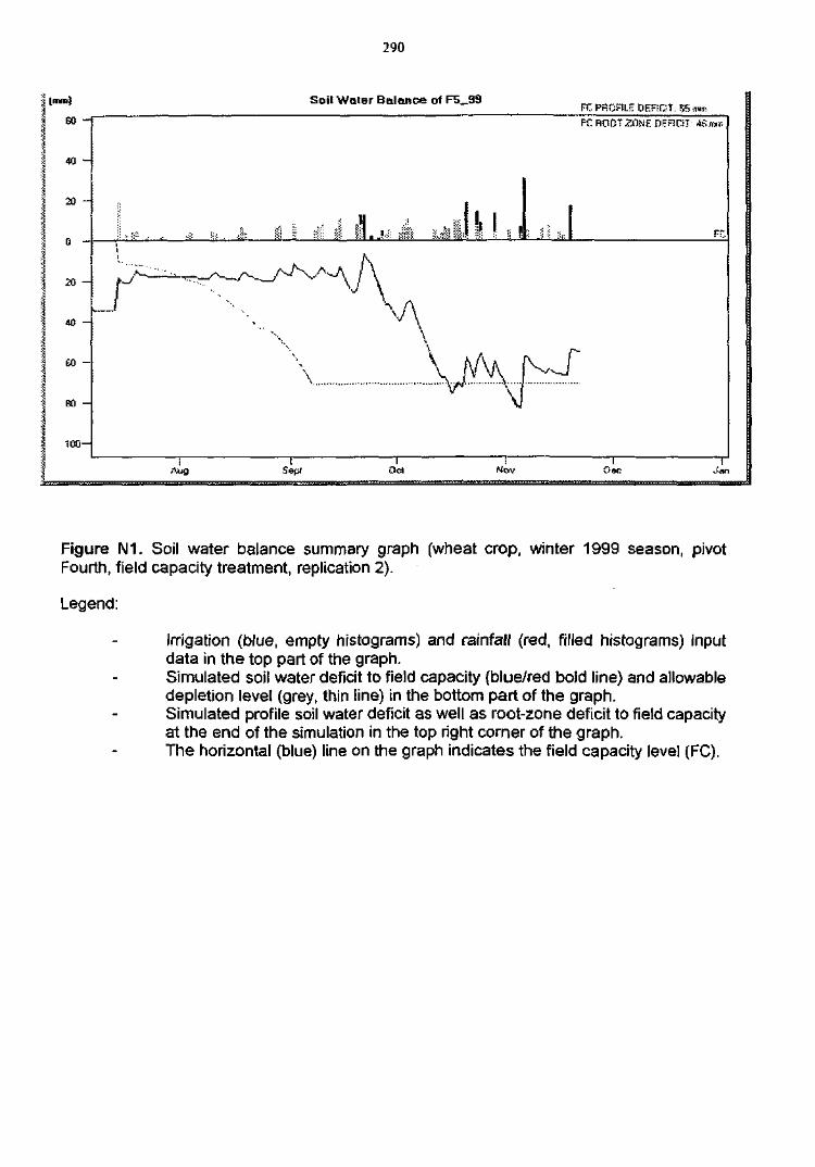
290

Soil Waler Balance of F5_39

FC ROOT 7XIH1. DEFICIT ASmr.

1 0 0 -

Augf

Sep; Oc! Hov

Figure N1. Soil water balance summary graph (wheat crop, winter 1999 season, pivotFourth, field capacity treatment, replication 2).

Legend:

Irrigation (blue, empty histograms) and rainfall (red, filled histograms) inputdata in the top part of the graph.Simulated soil water deficit to field capacity (blue/red bold line) and allowabledepletion level (grey, thin line) in the bottom part of the graph.Simulated profile soil water deficit as well as root-zone deficit to field capacityat the end of the simulation in the top right corner of the graph.The horizontal (blue) line on the graph indicates the field capacity level (FC).

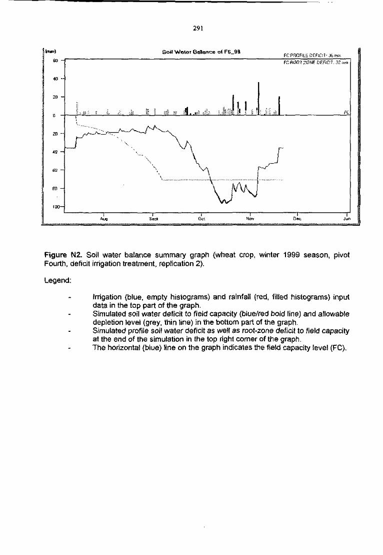
291

I™.) Soi l Water Ba ionce o< FE_99

60 H

20 -

FC ROOT ZOHF 0E?tC!T. 3? ;r,:u

100-

AygI

Set* NOT

Figure N2. Soil water balance summary graph (wheat crop, winter 1999 season, pivotFourth, deficit irrigation treatment, replication 2).

Legend:

Irrigation (blue, empty histograms) and rainfall (red, filled histograms) inputdata in the top part of the graph.Simulated soil water deficit to field capacity (blue/red bold line) and allowabledepletion level (grey, thin line) in the bottom part of the graph.Simulated profile soil water deficit as well as root-zone deficit to field capacityat the end of the simulation in the top right corner of the graph.The horizontal (blue) line on the graph indicates the field capacity level (FC).

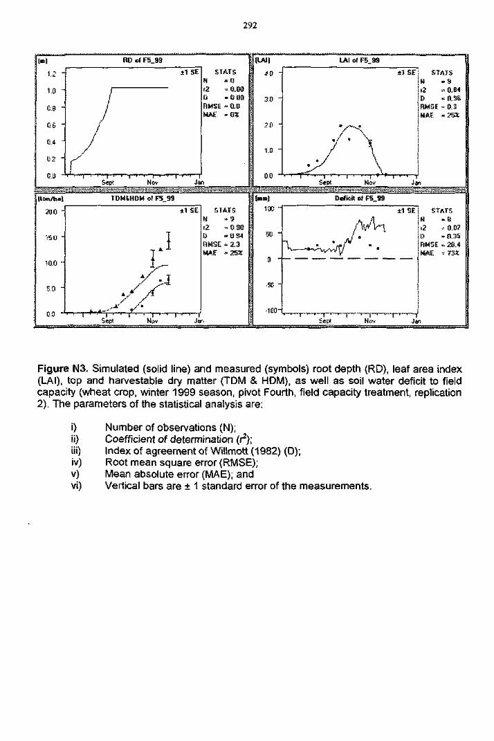
292

RD ol F5_99

STATSN - 0a •--• o.os

RMSE ••- o.oMAf - 0?

Sep! Nov

LAI of F5 99

* } SE i STATS

RMSE »0.3

0.0Sept Nov

0.0

TDMtHDM of F5 99

r.TATf, 100

Deficit or F5 99

•53 ~

Septi—[—'•

Nov-i"-^[—i 1—-V

Jan

Figure N3. Simulated (solid line) and measured (symbols) root depth (RD), leaf area index(LAI), top and harvestable dry matter (TDM & HDM), as well as soil water deficit to fieldcapacity (wheat crop, winter 1999 season, pivot Fourth, field capacity treatment, replication2). The parameters of the statistical analysis are:

i) Number of observations (N);ii) Coefficient of determination (r2);iii) Index of agreement of WHImott (1982) (D);iv) Root mean square error (RMSE);v) Mean absolute error (MAE); andvi) Vertical bars are ± 1 standard error of the measurements.

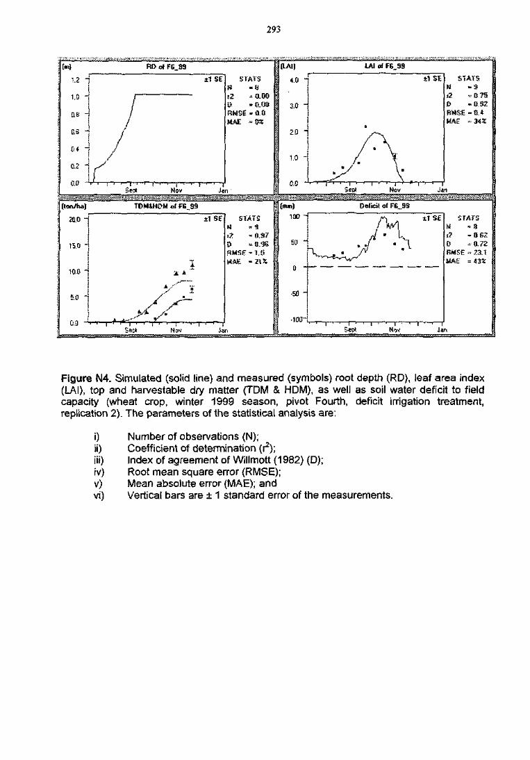
293

StATSH =3it -. 8 ?50 - a . 32BMSE - 0.4MAST - 342

Figure N4. Simulated (solid line) and measured (symbols) root depth (RD), leaf area index(LAI), top and harvestable dry matter (TDM & HDM), as well as soil water deficit to fieldcapacity (wheat crop, winter 1999 season, pivot Fourth, deficit irrigation treatment,replication 2). The parameters of the statistical analysis are:

i) Number of observations (N);ii) Coefficient of determination (r2);iii) Index of agreement of Willmott (1982) (D);iv) Root mean square error (RMSE);v) Mean absolute error (MAE); andvi) Vertical bars are ± 1 standard error of the measurements.

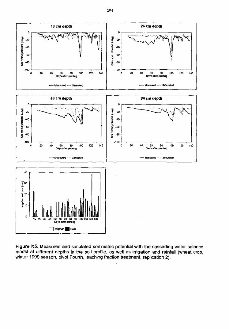
294

16 cm depth

o

-20

-40I

= -80

-10020 40 60 SO 100 120 140

Days after planting

-Measured Simulated

26 cm depth

o

-20

-40

o .60

-10020 40 60 80 100 120 140

Days alter planing

-Measured Simulated

0

-20

-40

E " 6 0

iI -80

-100

46 cm depth

20 40 60 SO 100 120 140Days after planting

- Measured •• •• Simulated

84 cm depth0

1 - 2 0"a

u -60

1% -30m

-10020 40 60 80 100 120 U0

Days after planting

— Measured Simulated

40

| 3 0

| 2 0

g

I.

10 20 30 40 50 60 70 80 90 10D110120 130Days aner planting

| | Irrigation ^ Rain

Figure N5. Measured and simulated soil matric potential with the cascading water balancemodel at different depths in the soil profile, as well as irrigation and rainfall (wheat crop,winter 1999 season, pivot Fourth, leaching fraction treatment, replication 2).

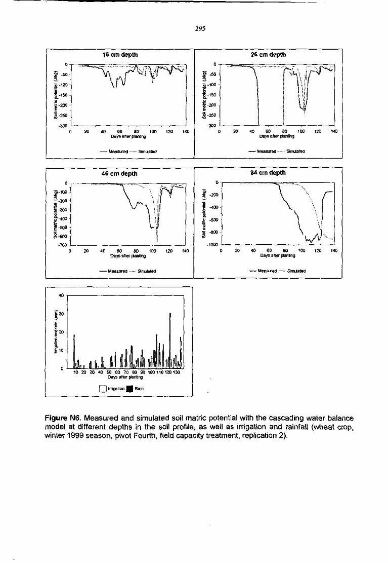
295

16 cm depth

40 60 80 100 120 140Days after planting

— Measured Simuated

26 cm depth

i\f

1

20 40 60 60 100 120 140Days after planting

-Measured • Simulated

0

a - 1 0 0 •

~-20Q •

f-3O0 •

-400

! - 5 0 0 ••

!-600-

- 7 0 0 ••

0

8.

46 cm depth

M|

20 40 60 80 100 120 140Days after planting

— Measured Simulated

84 cm deptho

-200

" 4 0 0

-600

-8D0

-1QD0

r

20 40 60 SO 100 120 140Days after planing

- Measured — Simulated

40

130

! 20

110

10 20 20 40 60 60 TO 60 90 100 110120130Days after planting

| | Irrigation ^ | Rain

Figure N6. Measured and simulated soi! matric potential with the cascading water balancemodel at different depths in the soil profile, as well as irrigation and rainfall (wheat crop,winter 1999 season, pivot Fourth, field capacity treatment, replication 2).

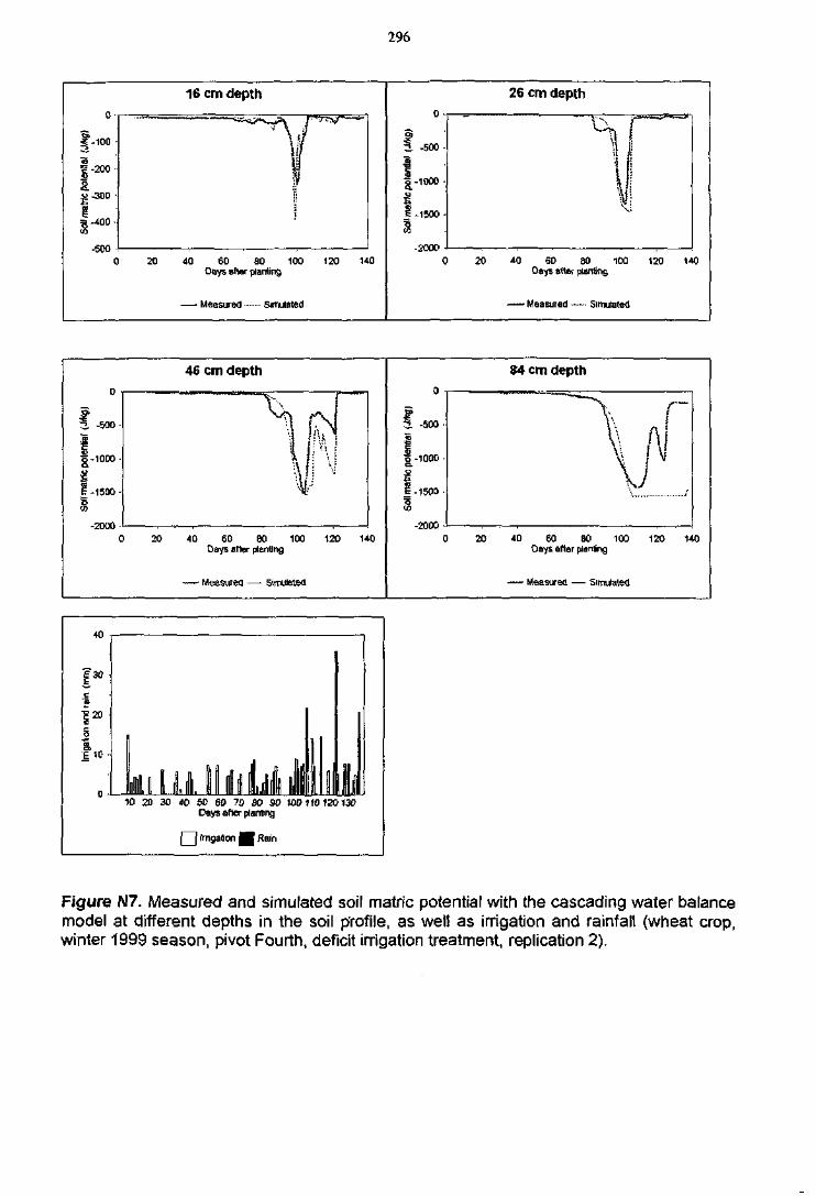
296

5

| - 2 0 0

J-300

^-<O0-

-500

16 cm depth

20 40 60 80 100 120 140Days after planting

• Measured Simiialed

0 - r

3 . -500 •

| - 1 0 0 0 -

i-1500 -

-2000

26 cm depth

20 40 60 BO 100 120 140Days after planting

- Measured Simulated

72 -500

[-1000

-1500-0w

-2000

46 cm depth

20 40 60 80 100 120 140Days after planting

- Measured — Simulated

34 cm depth

20 40 60 30 100 120 140Days after planting

Measured — Simulated

ID 20 30 40 50 60 70 SO 90 100 110 120 130Days after planting

Q (mgaaon ^ Rain

Figure N7. Measured and simulated soil matric potential with the cascading water balancemodel at different depths in the soil profile, as well as irrigation and rainfall (wheat crop,winter 1999 season, pivot Fourth, deficit irrigation treatment, replication 2).

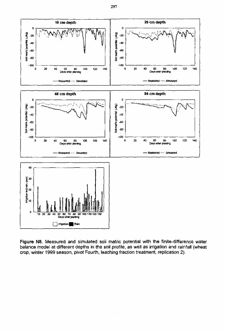
297

-100 -1-0

16 cm depth

20 40 60 BO 100 120 WODays after planting

- Measured Simulated

26 cm depth

-100

.'A,

20 40 60 SO 100 120 UODays after planting

— Measured Simulated

-100

46 cm depth

20 40 60 80 100 120 140Days after planting

-Measured Simulated

84 cm depth

40 60 60 100 120 140Days after planting

- Measured Simulated

40

|20

E 1 0 •

10 20 30 40 50 60 70 BO 90 100 110120 130Days after plans ng

( | Irrigation ^ Rain

Figure N8. Measured and simulated soil matric potential with the finite-difference waterbalance model at different depths in the soil profile, as well as irrigation and rainfall (wheatcrop, winter 1999 season, pivot Fourth, leaching fraction treatment, replication 2).

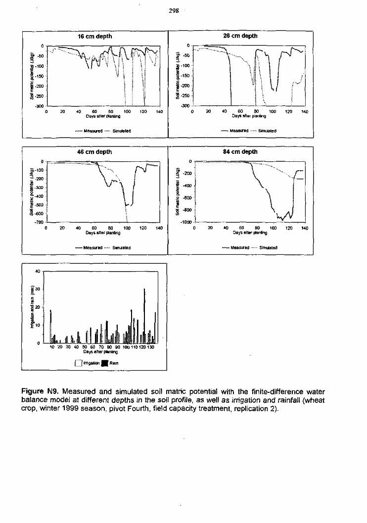
298

o

§ -50

75-100

I-200

5-250

-300

16 cm depth

20 40 60 SO 100 120 140Days after planting

- Measured Simulated

26 cm depth

o •

f -50

.5 -1O0 •

£ - 1 3 0 •

I -200 •

3-250-

-300 •

V.. f

U,SO 40 60 80 100 120 140

Days after Ranting

• Measured Sirnilatefl

0

B-100

r-200

| -300

u-400

g-50D

S-60D

-700

46 cm depth

v>

20 40 60 80 100 120 140Days after planting

- Measured Simulated

84 cm depth

0

I -200

-600

I" 8 0 0

-1000

-/I

2D 40 60 80 100 120 140Days after planting

-Measured Simuiaied

40

1 3 0

ICO

g

10 20 30 40 50 60 70 BO 90 100110120 130Days after planiing

( j Irrigation J | | Rain

Figure N9. Measured and simulated soil matric potential with the finite-difference waterbalance model at different depths in the soi! profile, as well as irrigation and rainfall (wheatcrop, winter 1999 season, pivot Fourth, field capacity treatment, replication 2).

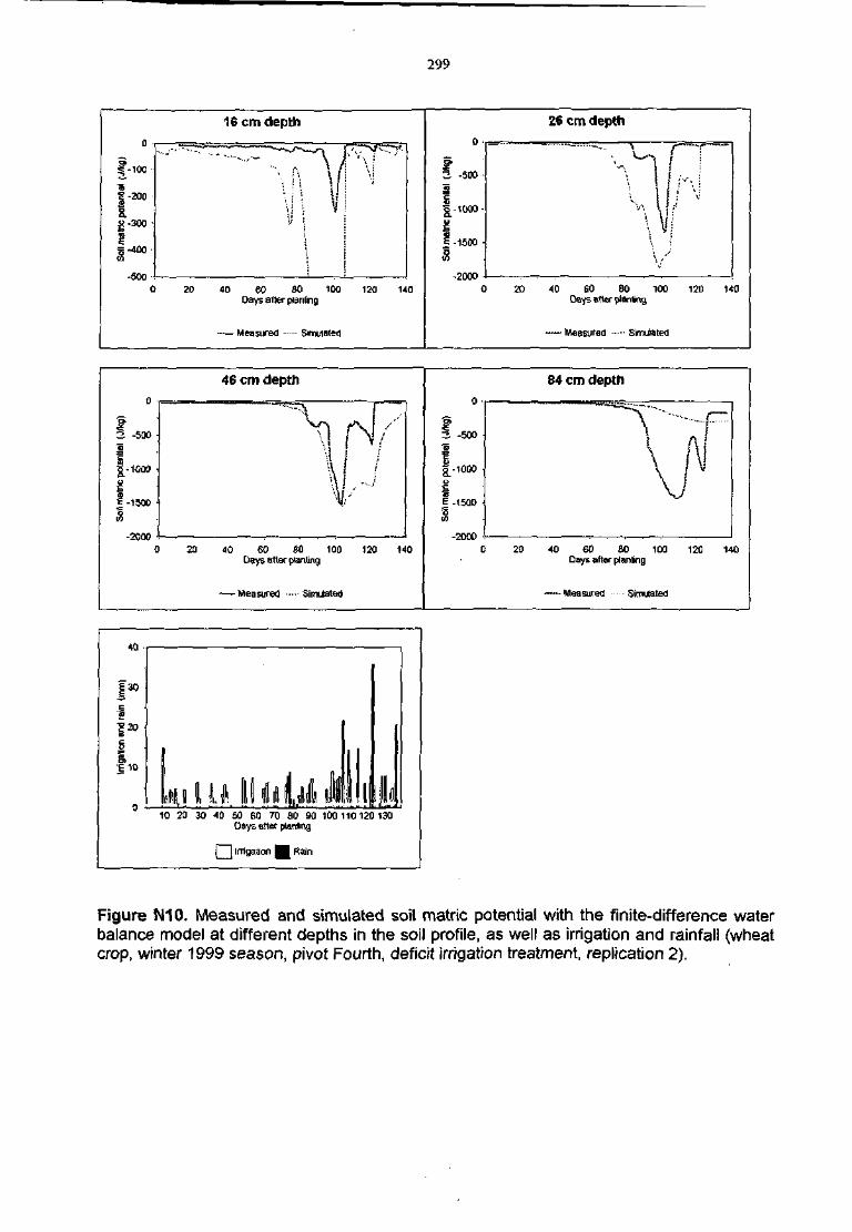
299

16 cm depth

I-200

" - 3 0 0

1I"4 0 0

-500-0 20 40 60 80 100 120 140

Days after planting

- Measured — Simulated

26 cm depth

3 -50O

1 -15D0 -

3-200O

0 20 40 60 80 100 120 140Days after planting

"Measured Sirraiated

3 -500 -m

|_-1000 •

I -1500 •

-2000

46 cm depth

20 40 60 60 100 120 140Days after planting

Measured Simiiated

84 cm depth

o

3 -500

£-1000

E. (500 •B10

-200D

20 40 60 80 100 12C 140Days after planting

-Measurod ---•• Simulated

:30

10 20 30 40 50 60 70 80 90 100 110120 130Days otter planting

j | Irrigation | Rain

Figure N10. Measured and simulated soil matric potential with the finite-difference waterbalance model at different depths in the soil profile, as well as irrigation and rainfall (wheatcrop, winter 1999 season, pivot Fourth, deficit irrigation treatment, replication 2).

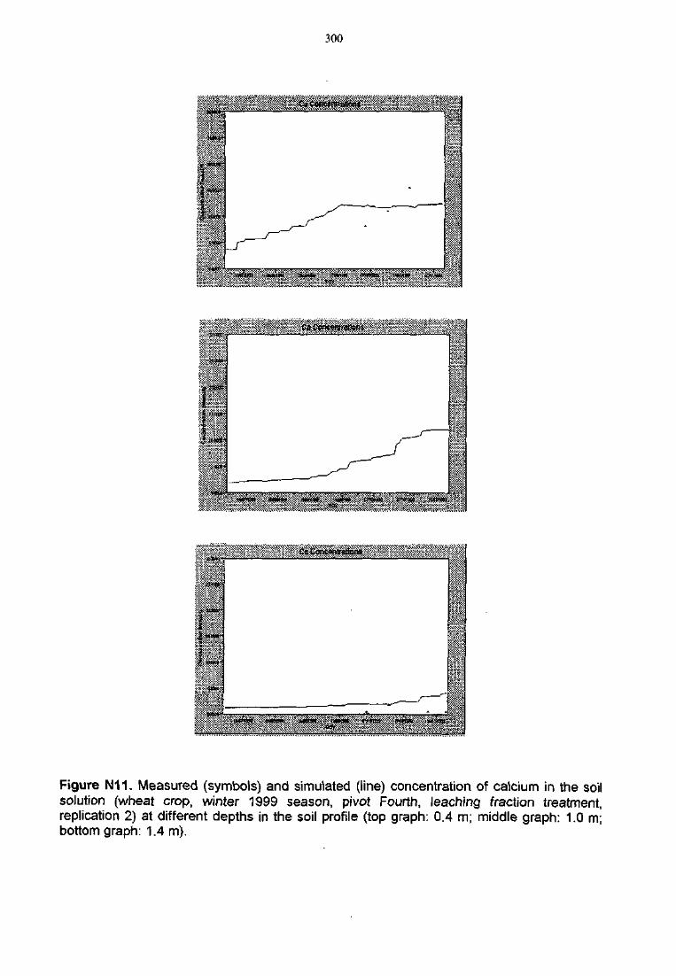
300

Figure N11. Measured (symbols) and simulated (line) concentration of calcium in the soilsolution (wheat crop, winter 1999 season, pivot Fourth, leaching fraction treatment,replication 2) at different depths in the soil profile (top graph: 0.4 m; middle graph: 1.0 m;bottom graph: 1.4 m).

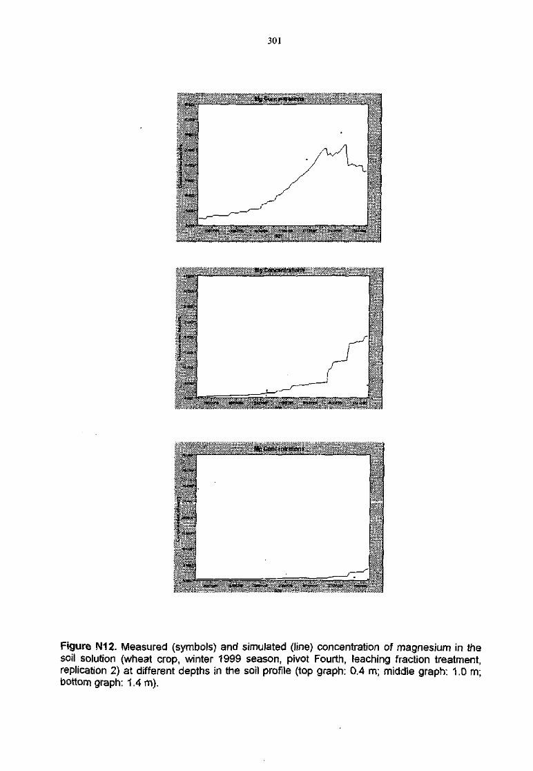
301

•SWft1-

+a;i>:sa Aaiiitb ' st&i*- ' »i>a«t lyssjff' * « i w -IKHW

Figure N12. Measured (symbols) and simulated (line) concentration of magnesium in thesoil solution (wheat crop, winter 1999 season, pivot Fourth, leaching fraction treatment,replication 2) at different depths in the soil profile (top graph: 0.4 m; middle graph; 1.0 m;bottom graph: 1.4 m).

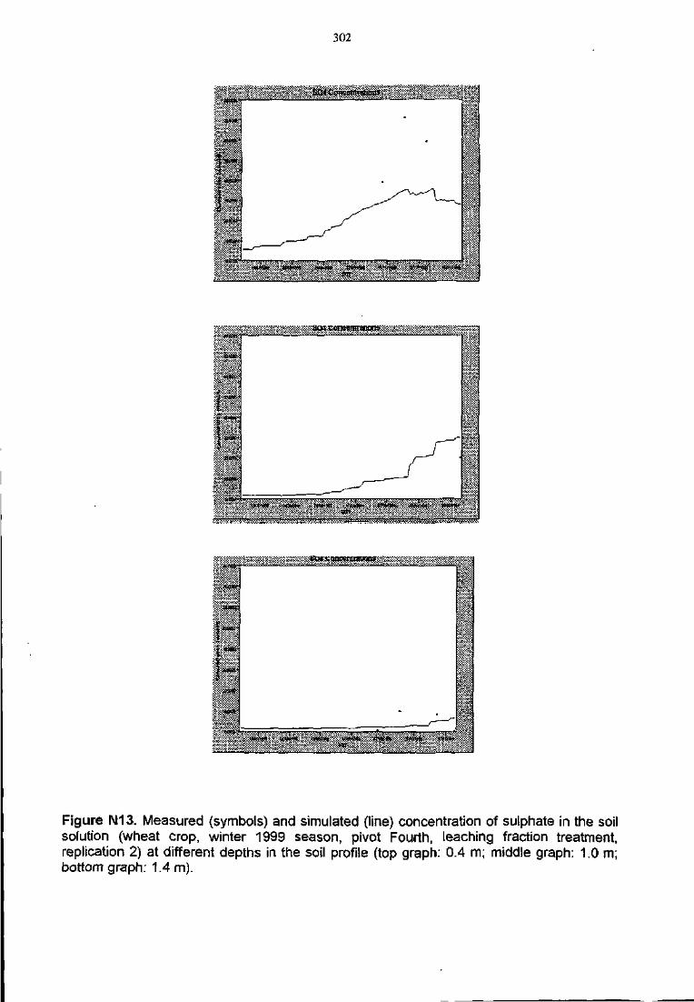
302

Figure N13. Measured (symbols) and simulated (line) concentration of sulphate in the soilsolution (wheat crop, winter 1999 season, pivot Fourth, leaching fraction treatment,replication 2) at different depths in the soil profile (top graph: 0.4 m; middle graph: 1.0 m;bottom graph: 1.4 m).

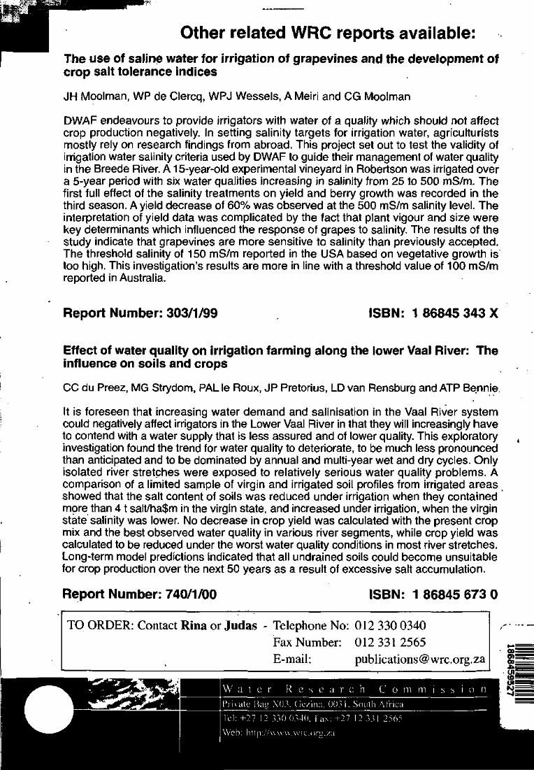
Other related WRC reports available:The use of saline water for irrigation of grapevines and the development ofcrop salt tolerance indices

JH Moolman, WP de Clercq, WPJ Wessels, A Meiri and CG Moolman

DWAF endeavours to provide irrigators with water of a quality which should not affectcrop production negatively. In setting salinity targets for irrigation water, agriculturistsmostly rely on research findings from abroad. This project set out to test the validity ofirrigation water salinity criteria used by DWAF to guide their management of water qualityin the Breede River. A15-year-old experimental vineyard in Robertson was irrigated overa 5-year period with six water qualities increasing in salinity from 25 to 500 mS/m. Thefirst full effect of the salinity treatments on yield and berry growth was recorded in thethird season. A yield decrease of 60% was observed at the 500 mS/m salinity level. Theinterpretation of yield data was complicated by the fact that plant vigour and size werekey determinants which influenced the response of grapes to salinity. The results of thestudy indicate that grapevines are more sensitive to salinity than previously accepted.The threshold salinity of 150 mS/m reported in the USA based on vegetative growth istoo high. This investigation's results are more in line with a threshold value of 100 mS/mreported in Australia.

Report Number: 303/1/99 ISBN: 1 86845 343 X

Effect of water quality on irrigation farming along the lower Vaal River: Theinfluence on soils and crops

CC du Preez, MG Strydom, PAL le Roux, JP Pretorius, LD van Rensburg and ATP Bennie

It is foreseen that increasing water demand and salinisation in the Vaal River systemcould negatively affect irrigators in the Lower Vaal River in that they will increasingly haveto contend with a water supply that is less assured and of lower quality. This exploratoryinvestigation found the trend for water quality to deteriorate, to be much less pronouncedthan anticipated and to be dominated by annual and multi-year wet and dry cycles. Onlyisolated river stretches were exposed to relatively serious water quality problems. Acomparison of a limited sample of virgin and irrigated soil profiles from irrigated areasshowed that the salt content of soils was reduced under irrigation when they containedmore than 41 salt/ha$m in the virgin state, and increased under irrigation, when the virginstate salinity was lower. No decrease in crop yield was calculated with the present cropmix and the best observed water quality in various river segments, while crop yield wascalculated to be reduced under the worst water quality conditions in most river stretches.Long-term model predictions indicated that all undrained soils could become unsuitablefor crop production over the next 50 years as a result of excessive salt accumulation.

Report Number: 740/1/00 ISBN: 1 86845 673 0

TO ORDER: Contact Rina or Judas - Telephone No:Fax Number:E-mail:

012 330 0340012 331 2565publications @ wrc. org. za

W a t e r R e s e a r c h C o m m i s s i o nPrivate Bag X03, Gezina, 003 i, South Africa

Tel: +27 12 330 0340, Fax: +27 12 331 2565

Web: http://www.vvrc.org.za

i