THE INDUSTRIAL INSTITUTE FOR ECONOMIC AND SOCIAL RESEARCH

WORKING PAPER No. 463, 1996

LECTURE NOTES ON INTERNATIONAL TRADE AND IMPERFECT COMPETITION BY ANTHONY VENABLES

Revised, 18/6/96

Lecture Notes on International Trade and Imperfect competition.

Contents: 1. Introduction

Anthony Venables

London School of Economics Houghton Street

London WC2A 2AE

2. Oligopolistic competition 2a: Price competition 2b: Quantity competition 2c: Trade policy 2d: Entry and exit. 2e: Segmented or integrated markets

3. Product differentiation and monopolistic competition. 3a: The model 3b: Factor endowments and the integrated equilibrium 3c: Trade costs and market access 3d: Regional economie integration 3e: Combining factor endowments and market access 3f: Factor prices, factor mobility and 'neweconomic geography'.

4. Concluding comments

l. lntroduction:

In the last fifteen years imperfect competition has come to the fore in the theoretical

analysis of international trade. This development was driven by a number of factors.

Researchers were motivated by the large and growing volume of international trade in similar

products (intra-industry trade) between similar countries, a phenomenon not adequately

explained by traditional theory based on perfect competition. They were also motivated by the

fact that many of the important commercial policy questions seemed to be better answered by

using tools from industriaI economics than from trade theory. And on the supply side,

developments in game theory and the theory of industrial organisation opened up a new set of

tools to be used by researchers.

The theory that has been developed over this period succeeds in providing a fuller

explanation of recent developments in trade flows, and also supports a rich set of policy

analyses, linking trade and industrial policy, and illuminating economic integration. It is

noteworthy that the theory can be integrated with the more traditional factor endowment and

general equilibrium concerns of trade theory; in some circumstances it can be placed 'on top

of' traditional theory, providing a theory of both inter- and intra-industry trade. It also opens

the way to constructing a theory of 'new econornic geography' , incorporating the location

decisions of finns and of mobile factors of production.

The objective of these notes is to provide an overview of the main developments in this

literature, and a framework within which the reader may place other work. The notes are

divide into two main sections. In the frrst our attention is on strategic interaction between

frrms in oligopolistic markets. The focus is on a single industry in which there are rather few

fmns, and the analysis can perhaps be described as 'open economy industrial economics'. We

investigate the trade flows that can occur in such an environment, and look at the welfare and

policy issues raised by this trade. In the second section we return to the general equilibrium

concerns of traditional trade theory. To capture these a simpler modeI of imperfect

c

cOlnpetition is needed -- we use the Spence-Dixit-Stiglitz framework which ignores strategic

interactions, and focuses on market power derived from product differentiation. Here our

primary concern is the pattern of trade, and we develop a complete synthesis of factor

endowment and market access determined trade flows. We also look at factor mobility, and

the possibility that this may lead to the agglomeration of economic activity.

2. Oligopolistic interaction:

lf fInns from different countries compete on international markets that are less than

perfectly competitive, then what form does their competitive interaction take? What trade

flows does it create? And what are the welfare effects of trade and of trade policy'! To

answer these questions we devote this section to the study of markets in which there is

strategic interaction between fInns.

As is of ten remarked, whereas there is only one theory of perfect competition, the

problem with imperfect competition is that there are many theories. These theories are unilled

in their use of modern game theory -- we shall be analysing Nash equilibria -- but differ

principally in their specification of the strategic variable chosen by fInns. In the following two

sub-sections we shalllook first at the case where fums' strategic variables are price, and then

when they are output or sales quantities. In a Nash equilibrium no firm has an incentive to

change'the value of its strategic variable given the values selected by other fums. However, as

we shall see, the equilibriurn can be quite different according as to whether prices or quantities

are chosen.

The difference between price competition (Bertrand) and quantity competition

(Cournot) is weIl known from industrial organisation. In the international trade context a

further distinction becomes important. Firms may choses quantities (or prices) in each market

separately, which will shall refer to as the case of segmented markets. Or they may select a

single world-wide quantity (or price), which we shall refer to as integrated market(). We shall

2

focus on the segmented market case, merely commenting on the difference made by integrated

markets.

Before undertaking formal analysis of these situations, it is convenient to specify some

of the notational conventions which will be followed throughout the paper. Subscripts i, j = l,

2... will be used to denote countries. In some con texts it is necessary to distinguish a variable

both by its origin and destination country, and the fust subscript will then denote origin and

second destination, thus x12 is a quantity produced in l and sold in 2. If a single subscript is

used then it should be dear from the context whether it refers to the location of consumption

or production. We shall sometimes refer to country 1 as 'home' and country 2 as 'foreign'.

2a: Price competition:

The simplest framework we can consider is a single industry containing one fum in

each country, l and 2. These firms have constant marginal costs, denoted cI and c2

respectively, for produeing ahomogeneous product We shall assume that markets are

segmented, so will look at just one country's market (there is no interaction between the two

markets, so the other market can be described analogously). We shalllook at the country l

market and suppose that there is a trade eost, t per unit, that the ftnn in 2 must incur if it is to

supply country l, making its effective marginal cost c2 + t.

Eaeh ftnn ehooses its price, PI or P2' What does the equilibrium look like, and does it

involve trade? Since both fums produce the same homogeneous product, all sales will go to

whichever frrm has the lowest price. If D(.) is the market demand function, we therefore have

demands faced by each frrm,

if PI > P2' Xl = 0, X2 = D(P2)'

if P2 > PI'

if PI = P2'

X2 = 0, Xl = D(Pl)'

Xl = X2 = D(PI)/2.

3

(1)

(the equal division of the market given in the last case is arbitrary).

Finns maximise profits, and their best response functions are illustrated on figure 2.1

by the functions RI(P2) and RipI)' PI = RI(P2) gives the values of pj that maximise finn l's

profits given the value of P2' Its shape is determined by the fact that profit maxirnisation

implies that firm 1 should just undercut firm 2 and thereby take the entire market, but never set

price less than ite;; uni t costs, cJ, or above the monopoly price pt. R2(PI) is constructed

analogously.

The Nash equilibrium is at the intersection of these best response functions, at point E.

What is the pattern of trade at this point'! The figure is constructed with the assumption that

c2 + t > el' The equilibrium involves prices PI = e2 + t - ö (where ö is a small positive

number), P2 = e2 + t, and therefore frrm 1 taking the entire market -- so there is 110 trade.

Notice however, that the possibility of trade affects the equilibrium. If trade were impossible,

then the market priee would be pt. The possibility of imports disciplines the domestic finn,

reducing its priee and profits, and raising overall social welfare -- the 'pro-competitive' effeet

of trade.

What is optimal trade policy in this model'] To answer this question suppose that t is

not a real trade eost, but a tariff, creating revenue which is transferred to the country 1

government. If e2 ~ el then welfare is maximised by setting t = el - e 2 + ö, where ö is a

small positive number. This value of t has two properties. First, at this value of t,

e2 + t '> e I ; this means that the domestic (country 1) firm (by assumption the lower eost

supplier) takes the entire market. Second, the domestic frrm is induced to set priee equal to it.;;

marginal eost, ej, beeause PI = e2 + t - Ö = el' Notice that this is an import subsidy, used

to tighten the competitive discipline on the home firm; of eourse, the subsidy is not aetually

paid (there is no trade in equilibrium).

If e2 < el then the optimal policy is t = cI - Cz - Ö. The foreign (country 2) firm

will then take the entire market at prlce P2 = e2 ~. t = C I - ö, Le. just less than th~

4

minimum price at which the domestic flfm is willing to supply. This policy generates tariff

revenue, so the unit eost of imports to eeonomy l as a who le is the eonsumer price minus

tariff revenue, P2 - t = c2 ' whieh is the world minimum production cost. The policy

therefore amounts to letting the lowest eost produeer supply the market (through imports),

but using the tariff to extract any profits that the importer might make.

Bertrand competition with homogeneous products is notorious for giving very sharp

and extreme results, and this is what we see in this case. Although quite illuminating, the

model fails to predict intra-industry trade, and effeets are probably too extreme to give an

adequate representation of many industries. We now tum to a case where the sharp price

under-cutting of Bertrand competition does not take place.

2b: Quantity competition:

We keep the same fmu and country structure, but now suppose that firrns use

quantities -- levels of sales in each market -- as strategic variables. This is the 'reciprocal

dumping' model of Brander and Krugman (1983).

Profits earned by each firrn in market l can be expressed as:

1t I = P(xI + X2)XI - C1Xl'

1t2 = P(x} + X 2)X2 - (e2 + t)x2•

where (XI + x2J is total sales in the market, and P(xI + x2) is the inverse dem and function

associated with D(p J.

(2)

To find the Nash equilibrium in quantities (Coumot) we look at eaeh firm's profit

maximising quantity choice given the quantity choice of other frrms. Profit maximisation gives

first order eonditions,

5

a1t 1 = P(XI + X2) ap

- el = O, +X-ax\ I ax

I

(3)

a1t2 - P(X + X2) ap

+X- -e -t=O aX2

- l 2 aX2

2 '

1 ap (XI + X2) • Since the elasticity of demand, E, is defined as - - = -. , and defmmg market

E ax p

shares mi as mi == Xi / (Xl + X2) these reduce to the usual form of the equality of marginal

revenue to eost,

P(X1 + x,)( 1 - :1) = el'

Plxl + x,)( 1 - ';) = e, + t.

(4)

Equilibrium is given by values of xJ and x2 satisfying these equations.

How does this compare with price competition'l The first point is that, even if

CI * c2 + t, both fInns can supply the same market Both finns receive the same price, but

the higher cost finn has smaller market share (lower mi)' this raising the elasticity of its

pereeived demand eurve (reducing mJE) and raising marginal revenue. (There is of course a

bound on the eost difference associated with both supplying the same market, which can be

computed easily from the eonditions above). A corollary of this is that the model supports

intra-industry trade. Both firms supply both markets, even if there are trade costs associated

with trade. The identical product is therefore 'cross-hauled' -- shipped in opposite direetions

by the two firms. o

What about the welfare implications of this trade? Trade has a pro-competitive effect,

reducing the price charged in each market, and this is a source of welfare gain. However,

trade also reduces profits, and may redlstribute them between countries. It tums out that trade

6

does not necessarily raise welfare, as demonstrated by the next two examples.

In this partial equilibrium framework we take as welfare criterion the sum of domestic

consumers' surplus, profits accruing to the domestic finn, and domestic government revenue

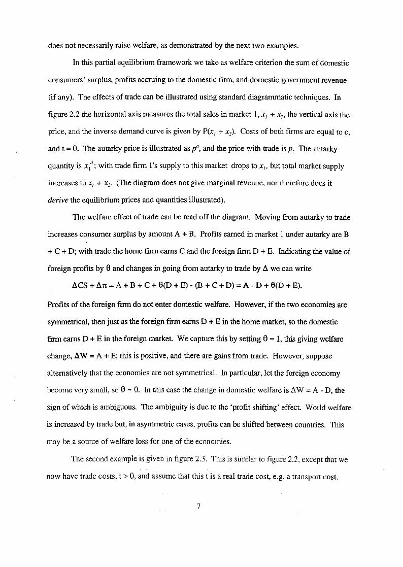
(if any). The effects of trade can be illustrated using standard diagrammatic techniques. In

figure 2.2 the horizontal axis measures the total sales in market l, Xl + x2, the vertical axis the

price, and the inverse demand curve is given by P(xI + x2). Costs of both finns are equal to c,

and t = O. The autarky price is illustrated as po, and the price with trade is p. The autarky

quantity is x1a

; with trade fum l's supply to this market drops to Xl' but total market supply

increases to Xl + x2• (The diagram does not give marginal revenue, nor therefore does it

derive the equilibrium prices and quantities illustrated).

The welfare effect of trade can be read off the diagram. Moving from autarky to trade

increases consumer surplus by amount A + B. Profits earned in market l under autarky are B

+ e + D; with trade the home finn earns e and the foreign finn D + E. Indicating the value of

foreign profits by S and changes in going from autarky to trade by fl we can write

fleS + fln = A + B + e + S(D + E) - (B + e + D) = A - D + S(D + E).

Profits of the foreign fmn do not enter domestic welfare. However, if the two economies are

symmetrical, then just as the foreign finn earns D + E in the home market, so the domestic

finn earns D + E in the foreign market. We capture this by setting S = l, this giving welfare

change, fl W = A + E; this is positive, and there are gains from trade. However, suppose

alternatively that the econornies are not symmetrical. In particular, let the foreign economy

become very small, so e-o. In this case the change in domestic welfare is fl W = A - D, the

sign of which is ambiguous. The ambiguity is due to the 'profit shifting' effect World welfare

is increased by trade but, in asymmetric cases, profits can be shifted between countries. This

may be a source of welfare loss for one of the econornies.

The second ex ample is given in figure 2.3. This is similar to figure 2.2, except that we

now have trade costs, t > O, and assume that this t is a real trade eost, e.g. a transport cost.

7

As before we can express changes in the domestic market as,

6.CS + 6.II = (A + B) + (C + F) + S(D + E) - (B + C + D + F + G)

where the first term is the change in consumer surplus, the second domestic profits, the third

foreign profits and the fourth the loss of profits that were earned under autarky. Looking at

the symmetric case, S = l, this reduces to 6. W = A + E - G which can be positive or negative.

The welfare effects are therefore ambiguous, even though the countries are iden tic al. The

reason for this ambiguity is that weighed against the pro-competitive gains from trade, are the

costs incurred in cross-hauling the product. It is possible to show that with Cournot

competition and homogeneous products the equilibrium involves more trade than is socially

optimal. Whether trade yields higher welfare than autarky is then, as we have seen,

ambiguous.

What we learn from these ex amples is that there is no general gains from trade theorem

in oligopoly modeis. It has of ten been argued that the gains from trade are larger under

imperfect competition than under perfect competition, because of pro-competitive effects.

This may well usually be the case, but there is no general theorem to that effect. As we have

seen, counter-examples can easily be constructed.

2c: Trade policy under imperiect competition:

In this subsection we look at both import and export policy for a country with one

domestic frrm and one foreign. In order to do this we frrst need to develop our welfare

criterion more fully.l

For country 1 the sum of domestic consumer surplus, firms' profit and governrnent

revenue can be written as:

The frrst tenn is the country l indirect utility function, measuring consumer surplus. We allow

for product differentiation, so the market l prices of both country I and country 2 fIfms enter

this function. The second is the profits of the country l finn in its home market, and the third

the profits of this finn on its sales in market 2. The last two terms are tariff revenue accruing

to the country l government, where a and p take values O or 1 depending on the policy

regime. If there is a country l import tariff at rate tz, then a = 1, transferring the tariff revenue

to country l. A country 1 export tax at rate tl implies p = 1.2

To analyse policy we shalllook at small ch anges in the equilibrium. Totally

differentiating (5) and using Roy' sidentity (dv/dPll = - XII' dv/dP21 = - X21 ) we derive:

dWI = - X21 dP21 + x 12dP l2 + (Pli - c)dxlI + (P12 - cI - fl (1 - P) )dx12 + af2dx21

+ aX2I df2 + (P -1)XI2dfI

(6)

The frrst two tenns give terms of trade effects on imports and exports respectively. The next

three are quantity changes times any wedge between marginal social benefit and marginal

social eost Marginal social benefit is price, and the marginal social eost of domestic

produetion is cost; notice that t/ is either a real eost or a transfer aecording as P = O or p = 1.

For imports, x2J' the unit eost to the economy is price, and there is a wedge on import supply

only if there is an import tariff, a = l. The fmal two terms are the direct effeet of the policy

change impacting on government revenue and, for a change in t/, also on profits.

Import tariffs: Consider the case of an import tariff, so dt2 > O, a = 1, dtl = O, P = O.

If markets are segmented and marginal cost curves are flat, then a country 1 import tariff will

have no effect on country 2 market variables, so dx12 = dpI2 = O. Equation (6) therefore

reduces to

(7)

These three effects are a terms of trade effect, (defined on the supply price), a 'finn expansion

9

effect' (an expansion of domestic production operating at price greater than marginal cost)

and a direct revenue effect.

The terms dp2I/dtz. d.xl/ldtz• d.x2l ldtz can be found by totally differentiating the

equilibrium conditions, and the expression can then be evaluated. We shall not go through the

details of this, but merely make some observations. Suppose we consider a small import tariff,

Le. dt2 > O around tz = O. The third term on the right hand side of eqn (7) is then zero. The

second is certainly positive because the tariff will expand domestic production, so creating

gains from a finn expansion effect. In the frrst term we must look at dP21 and dt2; the tariff will

usuallyraise the price, creating welfare loss, against which must be set the tariff revenue gain.

Combining these terms, what do we know about - XZI (dP2I - dtz)'? Notice first that, if marketo;

are segmented then even a 'small' country might experienee a change in this term; since prices

are set market by market rather than on a world wide 'integrated market' even small countries

can experience terms of trade effects. What of the sign of this term'? While it rnight be

expected that the price would increase by less than the tariff -- Le. the foreign finn absorbs

some of the tariff -- this need not be so. The policy may shift the industry to a less elastic part

of the demand curve, causing a large increase in p I' and making this term negative.

Overall then, we cannot be sure about the welfare effects of a tariff. There are gains

from the frrm expansion effect, and even small countries may be able to change their terms of

trade -- but the direction of this change is ambiguous.

Export taxes: lmposition of an export tax is a policy change dtl > O, P = 1, dt2 = O, ex

= O. The impact of this occurs in the country 2 market so d.xJJ =dXzI = dp21 = O and equation

(6) becomes,

(8 )

This says that the policy will raise welfare if it increases the surplus that country l takes from

10

country 2 -- either by increasing price, or expanding volume where price exceeds marginal

cost. Terms dplidt} and dx12/dtl can be found by totally differentiating the equilibrium

conditions, and the expression can be evaluated. However, a more direct approach is more

illuminating. We can express the surplus (profits plus tax revenue) country 1 derives from

sales in country 2 as W12'

(9)

The profits made by frrm l in market 2, 'Tt /2 , can be expressed as a function of the market 2

quantities supplied and the export tax, 'Tt 12(X I2, X22, t l ). Differentiating,

d'Tt 12 = a'Tt12 dx12

dt1 aX12 dt1

a'Tt12 dx22 +----aX22 dt1

(10)

In Cournot equilibrium the frrst term on the right hand side is zero, since x/2 has been chosen

to maxirnise 'Tt /2 given x22• In the fmal term, a'Tt1/at1 = - x12 from the defmition of profits.

Differentiating (9) and using (10) we therefore have,

(ll)

To evaluate the effects of a small export tax (i.e. around tl = O) we need only know a'Tt1/ax22

and dx2/dt1 • The former is certainly negative -- an increase in rival' s output reduces profits;

and the latter positive -- an export tax raises the rival's output. A small export tax therefore

reduces welfare and, conversely, a small export subsidy raises welfare.

This is the celebrated Brander-Spencer (1985) result, which has attracted so much

attention. In a competitive model subsidising export sales would always reduce welfare. Here

it has the opposite effect, essentially because the government, by committing to a subsidy, is

. able to secure a reduction in the foreign firm's output, X22" This is unattainable by the

Il

domestic fInn because -- by construction of the Nash equilibrium in quantities -- the domestic

fInn takes x22 as a constant.

The result has come in for a good deal of criticism as weIl as attention, and it turns out

not to be at all robust. Suppose that competition in the industry under study is intense, so the

industry is better characterised by a Nash equilibrium in prices than in quantities. We can

write profits as 1t \2(PI2' P22' t l ) and derive, analogous to (11),

(12)

But now a1t\2/ap22 > O and dP22/dtt > O -- an increase in rival's price raises profits, and an

increase in the export tax raises rival' s price. The optimal policy is therefore an export tax.

Results are reversed as we change the form of the game from quantity to price competition.

Whereas in Cournot competition government's power (relative to the home finn's) comes

from ability to induce a reduction in rival's quantity, it now comes from an ability to induce an

increase in rival's price. The former is achieved by an export subsidy and the latter by an

export tax. (This result is developed in Baton and Grossman (1986)).

The Brander and Spencer result is sensitive not only to the form of competition, but

also to the number of firms, to entry and exit possibilities, and to other aspects of the modeL

For example, increasing the number of domestic flIms in Cournot competition tums the

optimal policy from an export subsidy to a tax -- as we know it must when the number of

firms is large enough for the equilibrium to approach perfect competition. These and other

extensions are reviewed in Brander (1995).

d; Entry and exit:

So far we have held the number of flIms operating in each country constant. What

happens if entry and exit is possible'? Permitting the number of flIms to be endogenous is

12

important if theory is to explain 'long run' trade pattems. It also turns out to yield very dear

cut welfare and policy conclusions. (This section draws on the analysis of Venables (1985)).

We let the number of finns in each country be denoted nJ and n2' They all produce

homogeneous output so, using the inverse demand functions we can express prices in each

country as:

n J n2

PI = P(f:JXl~ + LX2~)' (13) k=1 k=1

where the superscript is an index labelling the finn, sums are over all finns in country l and in

country 2 and, for simplicity, we assume identical demand functions in both countries.

Profits of a representative finn in country 1 are

(14)

where the technology (common to all frrms in each country) has increasing return s to scale,

captured by constant marginal cost el and fIxed costiJ.

Given the number of frrms in each country we solve for Cournot-Nash equilibrium in

the usual way, by finding outputs implicitly defined by first order condltions of the form,

(15)

If all frrms in each country are synunetric then Xijk will be the same for all k, and we can drop

the superscripts. Solving for quantities gives the 'short ron' equilibrium -- i.e. the equilibrium

output levels and prices conditional upon the number of finns. We could use this information

to express 'short run' profits as a function of numbers of frrms, nI and n2, but it tums out to be

more insightful to make a different substitution. The short run equilibrium defines a . .. .'

relationship between numbers of firms and prices and, inverting this relationship, we can

13

express short mn profits as a function of prices p/and P2. We write this relationship II!VJ /,P2)'

IIip/,P2)·)

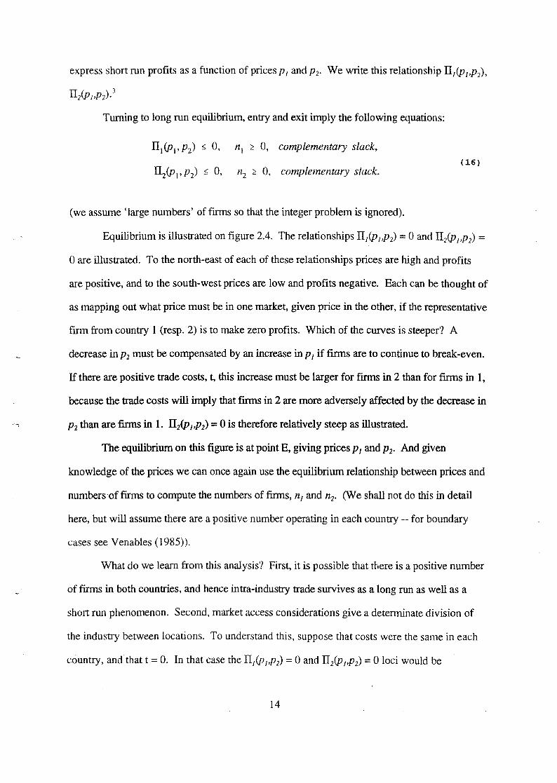
Turning to long mn equilibrium, entry and exit imply the following equations:

III (PI' P2) ::; O, nI ~ O, complementary slack,

II2(p1' P2) ::; 0, n2 ;:: O, complementary slack. ( 16)

(we asswne 'large numbers' of finns so that the integer problem is ignored).

Equilibrium is illustrated on figure 2.4. The relationships II/(p/,])2) = O and II2(P/,P2) =

O are illustrated. To the north-east of each of these relationships prices are high and profit 'i

are positive, and to the south-west prices are low and profits negative. Each can be thought of

as mapping out what price must be in one market, given price in the other, if the representative

finn from country 1 (resp. 2) is to make zero profits. Which of the curves is steeper'? A

decrease in P2 must be compensated by an increase in PI if finns are to continue to break-even.

If there are positive trade costs, t, this increase must be larger for finns in 2 than for finns in 1,

because the trade costs will imply that [mus in 2 are more adversely affected by the decrease in

pz than are finns in 1. IIip/,pz) = O is therefore relatively steep as illustrated.

The equilibrium on this figure is at point E, giving prices PI and pz. And given

knowledge of the prices we can once again use the equilibrium relationship between prices and

numbers-offirms to compute the numbers offirms, n/ and nz. (We shall not do this in detail

here, but will assume there are a positive number operating in each country -- for boundary

cases see Venables (1985»).

What do we leam from this analysis? First, it is possible that there is a positive number

of firms in both countries, and hence intra-industry trade survives as a long mn as weIl as a

short run phenomenon. Second, market access considerations give a detenninate division of

the industry between locations. To understand this, suppose that costs were the same in each

country, andthat t = O. In that case the II/(p/,P2) = () and II2(P/,P2) = () loci would be

14

identical, and we would not have a deternlinate division of the industry between locations. In

this mode l it is the presence of trade costs, t > 0, that gives the two curves different slopes.

Finns do relatively well in their home market, and hence price changes in their home market

have alarger effect on them than do price changes in their export market, and it is this that

.-gives the unique equilibrium at E. <We shall return to these market access considerations in

section 3c below).

The analysis also gives very clear cut results on gains from trade and trade policy. In

addition to giving trade prices at point E, the figure also illustrates autarky prices PIa and P2a

•

To see that these are autarky priees, notice that if P2 = 0, firms in l would make no profits in

market 2 and, to break even, require market l priee pt. Similarly under autarky -- no profits

are made in foreign market, so pt is needed in the home market to break even.

Comparison of the trade and autarky priees telIs us immediately that there are gains

from trade in this model. Free trade equilibrium prices are lower than dutarky priees in eaeh

country, so consumer surplus is higher. There are noprofits (because offree entry and exit)

nor govemment revenue, so changes in welfare are measured by changes in consumer surplus

alone. It is worth noting that these gains from trade come both from the pro-eompetitive

effects of trade and from increasing returns to scale. Trade increases eompetition, redueing

price, as in the oligopoly model of section 2b. With free entry and exit price equals average

eost, and the reduction in average cost is brought about by expanded firm seale. It is this

additional effect that guarantees the gains from trade.

What of trade policy? Consider an import tariff by country l. This is a tax on country

2 fums, so has the effect of shifting the II2(P/,P2) = ° loeus outwards -- the tax means that

fums in country 2 require higher priees if they are to break even. This shifts the equilibrium

point E to the right and downwards along the unchanged II/(p/,P2) = O Ioeus, reducing p/ and

raising p 2' A tariff therefore reduces the consumer price in the country that imposes it. The

reason for this perverse result is that the tariff,as a tax on foreign firms, reduces the

15

equilibrium value of n 2• This in tum raises the profitability of firms in l, and raises nI' With

positive t, and the consequent 'home market bias' in firms' sales, the net effect of these

changes is to increase supply to country 1 and reduce it to country 2, with the price effects we

have noted. The policy implications are immediate. Each country wants to increase its tariff

to secure the reduction in price (and, as a bonus, the tariff revenue). Of course, this policy is a

prisoners' dilemma for governments -- if pursued by both governments it would lead to

autarky, a position we know to be Pareto inferior to free trade.

The model also yields an unambiguous result on the effects of a small export subsidy.

A country l export subsidy benefits finns in 1, shifting the II/(p/,P2) = O locus inwards and

reducing p /; it can be shown that, for a small export subsidy, the benefit this brings outweighs

the direct revenue cost of the subsidy.

2e: Segmented or integrated markets.

We have so far maintained the assumption of market segmentation. How is the

analysis different if eompetition takes place in a single integrated market, i.e., eaeh firm

chooses a single value of the strategic variable for the world as a whoie']

In the ease of homogenous product price eompetition, it turns out that, if there are

transport costs, then no pure strategy equilibrium exists. Mixed strategy equilibria can be

found, and these support international trade with positive probability. (See Venables (1994».

Quantity competition in segmented markets is more straightforward, see Markusen (1981).

The results in the entry/exit mode l of section 2d depend critieal1y on the 'home market bias' of

sales, and this ceases to be apply if there is a single integrated market. Horstman and

Markusen (1986) and Markusen and Venables (1988) look at this ease.

Which assumption is the more appropriate? Presumably some offirms' strategic

variables are ehosen at a world wide level -- eg R&D, model range, and perhaps capacity -­

while others -- probably price -- are chosen at the level of particular markets. Ven;lbles (1990)

16

and Ben-Zvi and Helpman (1992) address this by looking at multi-stage games with different

decisions being taken at different leveis.

3. Product differentiation and monopolistic competition:

lo this section we tum to the literature on international trade in industries which are

monopolistically competitive, containing fmns that each produce a different variety of product.

The analytical structure is that of 'Spence-Dixit-Stiglitz' product differentiation in which the

industry has a large number of symmetric varieties. (See Dixit and Stiglitz (1977), Spence

(1976)). Firms gain market power from the fact that they are monopolists in their own

variety, and research ers typical1y make the sirnplifying assumption that this is the only source

of market power: finns ignore the effects of their actions on industry aggregate variables, so

that there is no strategic interaction between firms. The distinctions that were so important in

the preceding sections cease to be applicable.

This family of models has proved remarkably tractable, and it provides the basis of a

full general equilibrium synthesis of irnperfect competition and comparative advantage trade.

lo sectioD 3a we set out the basic model, and we do so in a tradition al two country, two

industry. two factor framework. In 3b we illustrate the Helpman-Krugman (1985) synthesis of

. comparative advantage and intra-industry trade, in which the location of production and

pattern of net trades is determined by factor endowments in a Heckscher-Ohlin fashion. In 3c

we look at the effects of trade costs on the equilibrium pattern of trade. If there are trade

costs the n 'market access' considerations become important in detennining the location of

industry -- fmns will want to locate in countries with large markets for their products. This

provides an alternative way of determining the location of industry and pattem of trade.

Section 3d uses this apparatus to study the effects of econornic integration, looking both at its

effects on the pattern of trade and on welfare.

The analysis of sections 3b and 3e provide alternative ways of detennining the location

17

of industry -- based on factor endowments and market access respectively. In section 3e we

develop the general theory in which both forces are present This has interesting implications

for international factor prices, and in section 3f these are analysed. It tums out that an

increase in economy's endowment of a factor may raise the return to that factor, meaning that

factor mobility is destabilizing. This approach provides a generalisation of Krugman's

(1991 a,b) work on econornic geography.

3a. The model.

As in section 2, the two countries are labelled 1 and 2, and country specific variables

are subscripted i, j = 1, 2. Each country is endowed with quantities L j and ~ of two factors,

the prices of which are w j and r j •

There are two production sectors. The z-sector is perfectly competitive and produces

output which is freely tradable and will be used as numeraire. Denoting the quantity of z

output in country i by ~ and its unit cost c(wj,r J, z sector activity satisfies,

Zi ~ 0, complementary slack, i = 1,2. (17 )

The x-sector is imperfectly competitive, containing firms that produce differentiated products.

We model product differentiation in the farniliar Dixit-Stiglitz manner, so can form a CES

price index for x-sector supply in each country, and we denote these price indices Si; this price

index can be thought of as a unit expenditure function for the x-sector alone. Consumer

preferences between sectors are described by a homothetic expenditure function defined on

the numeraire good and the x-sector price index, e( l ,s;Juj , where Ui is utility. In equilibrium,

income comes only from sale of factors, so the budget constraint takes the form,

e(l, s.)u. = wL. + r.K., I I I I I I

i = 1, 2. (18)

x-sector products can be supplied by national finns, the numher ofwhich in each

18

country is ni (i= 1,2). Country i finns set the same producer price Pi for sales in both markets,

but iceberg trade costs mean that to secure delivery of one unit the consumer has to purchase

1: units -- 1: - 1 units melt in transit. The prices paid for delivery of a unit to home and export

markets are therefore Pi and t:'fJi respectively. Each frrm produces a single distinct variety of

product, and we assume that, in each country, all finns are symmetric; we shall not introduce

notation to identify individual frrms. The quantities sold by a single finn in its home and

export market are denoted Xii and xij respectively.

Since market i is supplied by ni home finns, and nj foreign firms its price index for

differentiated products takes the form,

[ l-e ( )1-e]1/0- e) n.p· +n. 1:p. ,

l l J J i,j = 1,2, i '" j, (19)

where E is the elasticity of substitution between varieties, E > 1. The interpretation of this is

perhaps seen most easily by looking at the quantity index dual to Sj. Denoting this Yj, it is,

[(e -l)/e (e -l)/e J/(e-1)

Y· = n·x·· +nx·· , l 'u J IJ

i,j = 1,2, i '" j, (20)

Conditions for exact aggregation and the use of two-stage budgeting are satisfied, so the

product Sj Yj is equal to country j total expenditure on x-sector output. The quantity index can

be interpreted as a sub-utility function, giving the utility derived from consumption of x-sector

output. If E = 00, then all exponents would be unity, saying that products are perfect

substitutes (i.e. the industry produces a single homogeneous output) and the quantity index is

simply the total volume consumed. A finite value of E means that indifference curves between

varieties are convex, so consumers choose to consume all varieties available. We shall assume

that E > l, so that consumers benefit from the introduction of new varieties, as can be seen by

noting that the price index, Si' is decreasing in numbers of varieties on offer.

Using the price index in the expenditure function we can find the demand for each

19

variety of differentiated product. Shephard's lemma gives,

_ -E l-E E-l X·· -p. 1: s· E.

l] l l "

( 21)

E. == (wL. + r.K.) s.e (l,s.)/e(l,s.). l l l l l I S I I

Ej is country i expenditure on x-sector products in aggregate, and a subscript on a function

denotes partial differentiation. Although (21) gives quantities demanded, it should be noted

that the quantities of the traded goods consumed, cy' is

-E -E E-l C .. = JJ. 1: s· E.,

l] I I J (22)

The volume produced and shipped, xy, is 1: times greater than this, giving equation (21).

Technologies and profit maximisation are as follows. The profits of a single national

finn in country i are,

(23)

where b(wj , rj ) is marginal produetion eost, and b(wj , rj)! is fixed eost. Profit maximisation

gives priee,

(24 )

where Eij is the pereeived elasticity of demand for the finns sales in market j. The form this

takes depends on the nature of competition between firms. The Nash equilibrium in priees

has:

E .. = E(l-m .. ) + rim .. l] l] 'I lj (25)

where mij is the market share of a single finn from country i in market j, and" is the aggregate

iildustry elasticity of demand, Le. the elasticity of Yj with respect to Sj (we assume" >E). The

20

pereeived elastieity is therefore a weighted average of the elastieity of demand for the frrm's

own variety, E, and the elasticity of demand for the industry output in aggregate, 11. The Nash

equilibrium in quantities has:

E .. l]

(l - m .. ) m .. = __ -::.l]_ +-2.. (26 )

E 11

We shall frequently employ the 'large group' assumption, which says that market shares, mij,

are small enough to be ignored by firms. The pereeived elastieity of demand then reduees to

the parameter E.

Entry and exit of fInns ensures non-positive profits in equilibrium. If we make the

large group assumption, then price east mark ups are the same in both markets. Using the

prieing equation, (24) to eliminate Pi from the defInition of profIts we can therefore express the

industry equilibrium condition as,

f(E - 1) ~ Xii + Xij' ni ~ 0, complementary slack. (27)

Total sales must reach level f( e - l), where the values of Xii and xij are deterrnined by demand

equations (21). The power of the large group assumption is immediately apparent. With this

assumption ~ is simply equal to the parameter E, so equilibrium finn scale is a constant,

depending only on parameters of the model.

To complete eharacterization of equilibrium we need only specify factor market

clearing. This takes the form,

L. = z·c (w.,r.) + n,rx .. +x .. +/Jb (w.,r.) I I W I I IL Il lj w I l (28 )

K. = z.c (w.,r.) + n.[x .. + x .. +/Jb (w.,r.) I I r l I l Il l] r I I (29 )

21

The terms on the right hand side give factor demands associated with z-sector and with x­

sector production.

3b: Factor endowments and the integrated equilibrium

If there is completely free trade (r = 1) and we make the large group assumption, then

the model is that of Helpman and Krugman (1985). We can use the 'integrated equilibriurn'

approach to illustrate the equilibrium. Suppose that the world in not divided into two

economies, each with its own endowment, but is instead a single economy. We can fmd the

equilibrium of this economy, and we shall caU it the 'integrated equilibrium'. We find,

amongst other things, the techniques of production in use in each sector, and these labour

capital ratios will be denoted Az and Ax respectively. We shalllabel factors such that the x­

sector is capital intensive.

Now consider figure 3.1. The dimensions of the box are the world endowment, with

capital on the horizontal and labour on the vertical. We divide this between the two countries,

with origins for country l in the south west comer and country 2 in the north east A point in

the box therefore describes a division of the world endowment between the two countries.

We now pose the foUowing question. Suppose the world is divided into two countries,

and in particular, the endowment is divided between these countries. If factors are assumed

non-traded and good s are freely traded, can trade reproduce the integrated equilibrium? The

answer is yes, providing the endowments lie in the parallelogram formed by O,BOp. The

sides of this parallelogram are rays from the origins (both 0, and 02) with gradient equal to

labour capital ratios; operating the x industry therefore employs capital and labour in amounts

given by the line O,X, and operating the z industry employs capital and labour in amounts

given by the line O,Z. If the endowment is in the parallelogram then there are non-negative

output levels for each industry in each country whlch full Y employ both factors in both

22

countries. This means that the free trade equilibrium reproduces the integrated equilibrium -­

we have full employment of both factors at the same techniques of production and factor

prices, this generating the same costs and prices, income and demand, and supply of all goods.

The parallelogram is referred to as the diversification set, i.e. the set of endowments in

which both industries are active in both countries. In the case we are studying, with 1: = J,

trade can reproduce the integrated equilibrium if and only if the factor endowment lies inside

this set. If trade reproduces the integrated equilibrium then factor prices in the two countries

are the same, so the diversification set is also the factor price equalisation set.

Outside the diversification set the configuration is similar to that described by Dixit and

Norman (1980). If economy l is very labour abundant then nI = O, and if 2 is very capital

abundant, then Z2 = O. The dividing line between these regions is line AB. North-east of this

line economy 2 is not large enough to produce world demand for x-sector output, so we have

nI' n2 > O; south-west of the line economy l is not large enough to produce world demand for

z, so we have z/' Z2 > O.

If we restrict attention to the FPE set then the pattem of trade can be found easily.

Suppose the endowment is at E. The factor content of consumption will then be at

corresponding point e, constructed to satisfy two properties. First, e must lie on the main

diagonal. This is because countries have identical homothetic preferences, so they consume x­

and z- sector output in the same proportions; they must also therefore consume the factors

embodied in this consumption in the same proportions. Second, the position of e relative to E

is detennined by the fact that e lies on the line through E with gradient r/w. This is the budget

constraint, saying that the value of the endowment equals the value of factors embodied in

consumption.

The vector Ee is the difference between a country' s factor endowment and factor

content of consumption, and is therefore the factor content of its trade. As drawn, country l

is a net importer of capita! and exporter of labour, embodied in traded goods. This factor

23

content of trade is achieved by 1 exporting the labour intensive good, z, and importing capital

intensive x-sector products. The pattern of inter-industry trade is therefore exactIy as in the

Heckscher-Ohlin modeL

While inter-industry trade is as predicted in the Heckscher-Ohlin model, this model

also supports intra-industry trade. x-sector firms are operating in each country, and each frrm

sells its output in each country, at levels determined by the demand functions, equations (21).

The volume of this trade is largest if endowments in both countries are identical (the centre of

the endowment box). At this point there is no inter-industry trade (because relative

endowment5 are the same), and the x-sector industry is divided equally between the countries.

Each finn sells half its output in each country, meaning that half of x-sector output is traded

internationally.

c: Trade costs and market access.

The Helpman and Krugman analysis is an elegant synthesis of factor endowment and

intra-industry trade, but the assumption of completely free trade means that each importing

finn has exactIy the same market share as each domestic finn, implying that the volume of

trade may be as large as half the volume of output in a two-country model, or fraction (N-I)/N

the volume of output if there are N identical countries. This is an order of magnitude larger

than trade flows actually observed. How are things changed if we allow for a 'home market

bias' in sales, by introducing positive trade or transport costs, 1: > l ?

The equilibrium location of the industries must always satisfy two sorts of conditions.

The frrst are factor market conditions, stating that the industries must generate factor demands

sufficient to employ the factor supplies in each economy. The second are product market

conditions, stating that supply of output must equal demand in each economy.

If trade is completely free, as in the preceding section, then the product market

conditions are relaxed. World supply must equal world demand for each product, but -- from

24

the point of view of the product market -- the location of production is immaterial, as output

can be transported costlessly to supply either market This is the basis of traditional mode Is of

trade, as weIl as Helpman and Krugman. Providing trade is completely costless, the division

of industries between countries is determined by factor market, not product market

considerations.

If there are trade barriers, then we have to pay attention to supply and demand in each

market Expenditure levels in each market then also have a role in determining the location of

production -- other things being equal, countries with a large expenditure on the x-sector

industry will have a large volutne of production in this industry. To see this it is helpful to

derive an explicit equation for the value of x-sector production in each location. We can do

this as follows. Using the demand equations (21) in the zero profit condition (27) we obtain;

i,j=I,2, i#I (30)

We can solve these two equations to express the terms sr l Ej in the following fonn:

i,j = 1,2, i :F j. (31)

Suppose that factor prices are the same in the two countries, so p J = P2' and we denote the

common value [J. The x-sector price index (equation (19» can therefore be expressed as,

(32)

From (31) and (32) we obtain

~fJf(E-l) = (33)

. The left hand side of these equations is the value of x-sector production in countries 1 and 2

25

(recall that the zero profit level of output is attained at seale f{ c-l J). The equations tell us how

the value of produetion depends trade eost and expenditure levels in each country.

What do we leam from these equations? First, if there is completely free trade, 1: = l,

then the equations are not defined. As we have already seen, in this case the location of

production is determined entirely by factor supply, and product market access considerations

are irrelevant.

Second, if 1: > l (and hence l > 't l - E), then production is skewed towards the

location with the larger market. This is unsurprising, but a stronger result also holds.

Differences in expenditures lead to a proportionately larger difference in output leveis. To see

this, notice that production in country l relative to country 2 can be expressed (taking the

ratio of equations (33)) as

E/Ez - 't1- E

=-----, l - 't 1- E E/Ez

(34)

This relationship is illustrated in figure 3.2. There is production in both countries only if E/

E2 E ('t l-e. 't e-l). The relationship intersects the 45° line from below, illustrating that changes

in E/ E2 are assodated with proportionately larger changes in n/I n2• Furthermore, the

smaller is 't (larger is 't l-e) the steeper is the function indicating increasing sensitivity of the

location of production to expenditure differences.

This establishes that market size is a determinant of the location of production and

pattern of trade. Countries with large markets in a particular sector will have a

disproportionately high share of that sector's production, and will be a net exporter of that

product. The reason is market access -- firms will want to locate in the large marker. The

intuition can also be seen by considering what would happen if the relative location of

production was the same as the relative location of demand (n}/n2 =EJE2). The large

economy would the n have a lower import penetration ratio than the small, so entry of frrms

26

would be profitable in the large rather than in the small.

3d: Regional economie integration;

In sections 3e and 3f we shall synthesise factor market and market access theories of

the location of industry. In this section we digress to look at an application of this model.

What does it tell us about the effects of regional economic integration schemes'l We look flIst

at the positive effects of integration and show how it may cause 'production shifting' between

economies. We then tum to the welfare effects of integration. Fuller analysis of this topic is

provided in Baldwin and Venables (1995).

The positive effects of integration on the location of industry can be derived from the

analysis of section 3c. Suppose there are only two economies, and trade barriers between

these countries are reduced. As 't falls, which country gains industry? It can readily be shown

by differentiation of (34) that, if we take expenditure levels Ei as exogenous, then reductions

in 't shift industry towards the economy with the larger expenditure (the ni nz curve of figure

3.2 rotates anti-clockwise around the point (1,1). This is of course just an application of the

result that large economies will be net exporters of the product of the imperfectly competitive

industry. The result suggests that a process of economic integration may tend to draw activity

into countries or regions with good market access, at the expense of peripheral regions with

smaller local markets.

What of a preferential regional integration scheme? To analyse this we need a three

country model, in which two countries, the union members, have lower trade barriers with

each other than they do with the third country. Suppose that the two union members have the

same expenditure level, El' and that the third country has expenditure EJ. Iceberg trade costs

between union members are 't, and with the third country are 6. Proceeding analogously to

the derivation of equations (30) to (33) we can derive output levels in one of the union

countrles and in the third country as: .

27

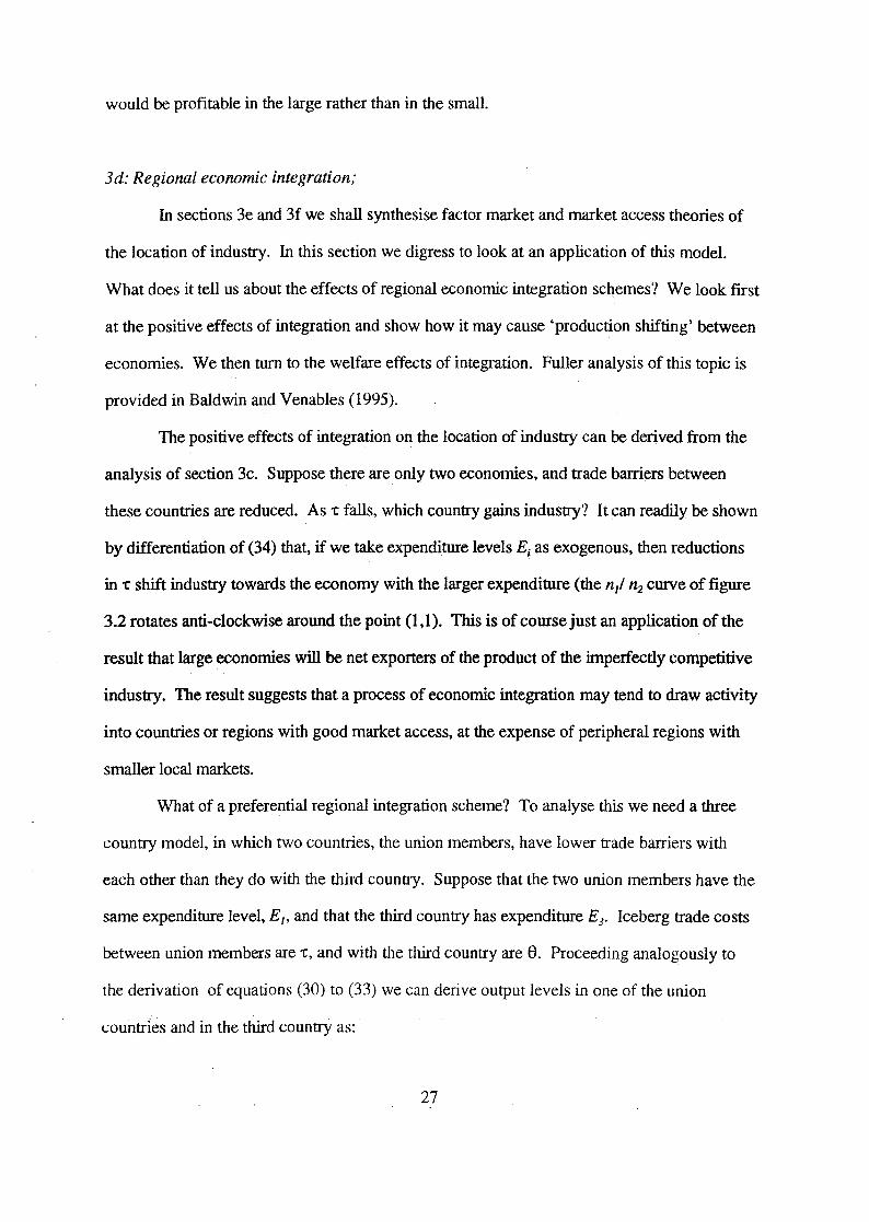
nI PfCE -1) =

E3

(1 + -c 1 -E) n3 pf(E-1) = -----­

+ -c 1 -E _ 281-E

(35 )

Differentiating these equations it can be shown that integration between 1 and 2 -- a

reduction in -c (in<"lease in -c lo€) holding 8 constant -- raises n j (=n2) and reduces n3• ln other

words, integration causes 'production shifting' into the union from third countries. It works

because'";integration raises the profits of finns in the union countries, attracting entry. But

these entrants also supply country 3, reducing profits of fIrrns located in country 3, causing

their exit which in tum attracts further entry in 1 and 2, and so on.

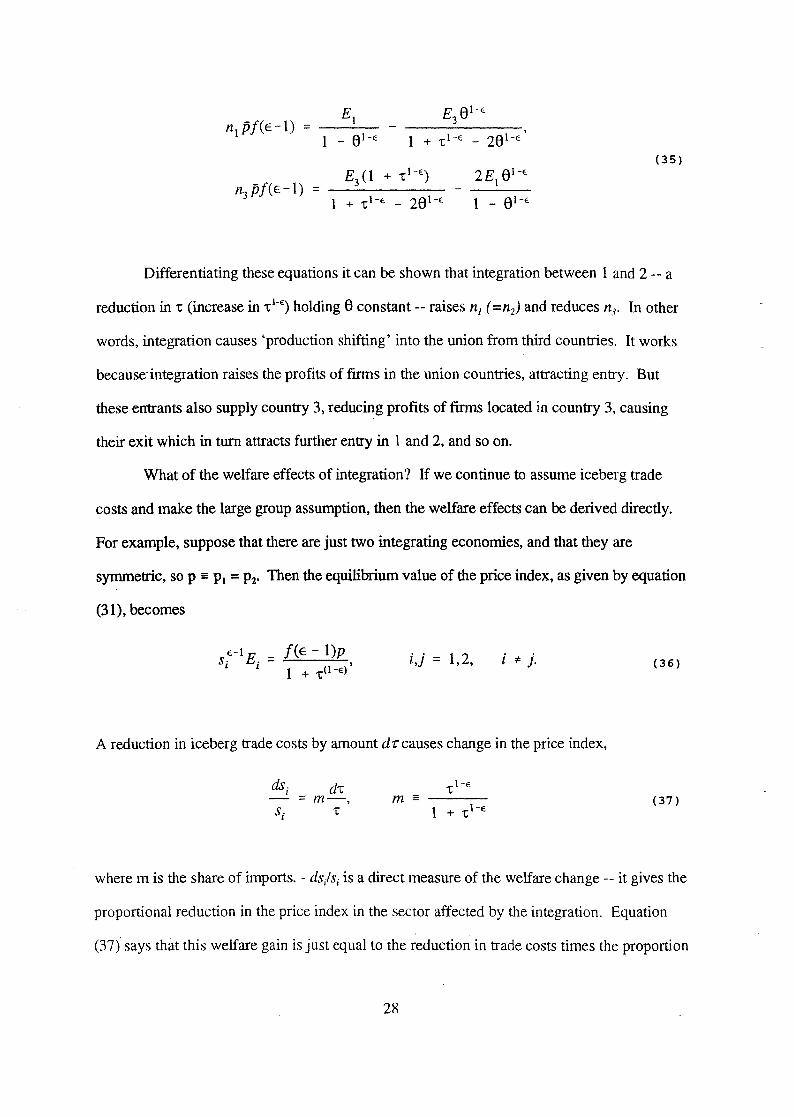
What of the welfare effects of integration? If we continue to assume iceberg trade

costs and make the large group assumption, then the welfare effects can be derived directly.

For example, suppose that there are just two integrating economies, and that they are

symmetric, so p == PI = PZ' Then the equilibrium value of the price index, as given byequation

(31), becomes

S:-l E. = fCE - 1)p , l l 1 + -C(1-E)

i,j = 1,2, (36)

A reduction in iceberg trade costs by amount dt"causes change in the price index,

dS i d-c =m-, (37)

Si -c

where m is the share of imports. - ds/sj is a direct measure of the welfare change -- it gives the

proportional reduction in the price index in the sector affected by the integration. Equation

(37) says that this welfare gain is just equal to the reduction in trade costs times the proportion

2X

of output directly affeeted by this reduetion. In other words, the only gain (to a frrst order

approximation) is the direet eost saving from the reduetion in the real trade eost Firm seale

does not ch ange (it is fIxed by the large group assumption) and the number of frrms operating

in the industry does not ehange (as can be seen by totally differentiating (32) and using (37».

This result is rather disappointing -- the absence of any indueed welfare ehanges in a

model of imperfeet eompetition is rather surprising. However, the result tums on two very

strong assumptions that have been employed -- iceberg trade costs and the large group

assumption.

Suppose that trade barriers take the form of tariffs, rather than real trade costs. The

effects in this case can be derived by using demand function (22) instead of (21) and we

derive, analogous to (37),

dsi E dr: = m----, Si E -1 t

t-€ m=--­l + t-€

(38)

where the import share, m, no longer includes the iceberg element The price index change is

larger in this case, essentially because the induced increase in trade volume no longer uses up

real resources. To calculate the welfare change we must also compute the change in

govemment revenue. If this is done, it can be shown that there is a net welfare gain from the

integration.

The 'large group' assumption serves to rule out any 'pro-eompetitive' effects of

economic integration. As we have seen, this assumption says that the pereeived elasticity of

demand is equal to the constant parameter, E. As weil as ruling out 'pro-eompetitive' effects,

this assumption also means that frrm size is constant, and unchanged by ch anges in t, so that

integration can bring no gains from fuller exploitation of return s to scale.

To relax the large group assumption we return to the pricing equations (24) - (26).

Integration ch anges market shares, mij' this taking the form of an inerease in each flrm's share

29

in export markets and a fall in its home market share. Under either quantity or price

competition this raises the perceived elasticity of demand in the home :narket and reduces it in

export markets, causing a reduction in price cost margins in the home market, and increase in

theses margins on export sales. How does this affect profits? If home sales are larger than

sales in each export market, then the net effect is a reduction in profits -- the reduction in

margins occurs on high volume and the increase on small. (For fuller analysis of this see

Baldwin and Venables (1995)). The reduction in profits causes exit of firms, and some loss of

product variety. However, it also expands the scale ofremaining firms, and reduces their

averagecosts. Integration therefore both increases the intensity of competition, as flIms

invade each others markets, and increases fum scale and reduces average costs, as there is a

change in the number of fums in response to the change in profit leveis.

Attempts to quantify these effects are given in Smith and Venables (1988). This paper

also investigates the implications of integration being associated with a change in the nature of

competition, switching the equilibrium from one with segmented markets to one with

integrated markets. H this were to occur then the market share terms in the pricing equations

would no longer be shares of each finn in each market, but instead shares of each finn in the

entire market of the union. This amplifies the effects we have just outlined. Firms lose

relatively protected positions in their domestic market, as competition takes place in the union

market as a who le.

3e; Combiningjactor endowments and market access;

We have seen in sections 3b and 3c that it is possible to determine the location of

industry in two different ways -- through factor endowments, in a Heckscher-Ohlin manner or,

if there are positive trade costs, through market access considerations. What happens when

we put these two approaches together?

The easiest way to address this question is to ask what happens to the FPE set when

30

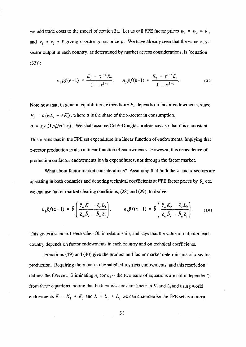
we add trade costs to the mode I of section 3a. Let us call FPE factor prices wl = w2 = w,

and r l = r2 = r giving x-sector goods price p. We have already seen that the value of x­

sector output in each country, as determined by market access considerations, is (equation

(33»:

(39)

Note now that, in general equilibrium, expenditure Ej, depends on factor endowments, since

E. = a(wL. + 'PK.), whereaistheshareofthex-sectorinconsumption, l I l

a == Si e/ l ,.s)/e(l ,Si)' We shall assume Cobb-Douglas preferences, so that a is a constant.

This means that in the FPE set expenditure is a linear function of endowments, implying that

x-sector production is also a linear function of endowments. However, this dependence of

production on factor endowments is via expenditures, not through the factor market.

What about factor market considerations'l Assuming that both the z- and x-sectors are

operating in both countries and den oting technical coefficients at FPE factor prices by bw etc,

we can use factor market clearing conditions, (28) and (29), to derive,

(40)

This gives a standard Heckscher-Ohlin relationship, and says that the value of output in each

country depends on factor endowments in each country and on technical coefficients.

Equations (39) and (40) give the product and factor market determinants of x-sector

production. Requiring them both to be satisfied restricts endowments, and this restriction'

defines the FPE set. Elirninating ni (or n2 -- the two pairs of equations are not independent)

from these equations, noting that both expressions are linear in Kj and L j and using world

endowments K = Kl + K2 and L = L, + L2 we can characterise the FPE set as a linear

31

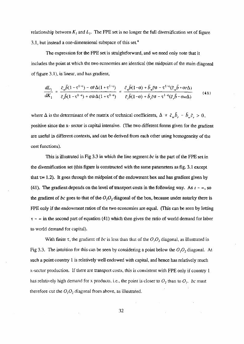
relationship between K/ and L/. The FPE set is no longer the full diversification set of figure

3.1, but instead a one-dimensional subspace of this set.4

The expression for the FPE set is straightforward, and we need only note that it

includes the point at which the two economies are identical (the midpoint of the main diagonal

offigure 3.l), is linear, and has gradient,

dL1 cjj(1 _-r 1-E

) - arÅ.(1 +-r h') cjj(1-a) + hwca - -r1-\cwh +an~.)

= = ------------------~-----dK l Crh(1 - -r 1-E) + aWÅ.(1 + -r l-E) C rh(1-a) + h rca - -r I-E(C rh - awÅ.)

(41)

where Å. is the determinant of the matrix of technical coefficients, Å. == cwhr - h c > O w r '

positive since the x- sector is capital intensive. (The two different forms given for the gradient

are useful in different contexts, and can be derived from each other using homogeneity of the

cost functions).

This is illustrated in Fig 3.3 in which the line segment be is the part of the FPE set in

the diversification set (this figure is constructed with the same parameters as fig. 3.1 except

that 1:= 1.2). It goes through the midpoint of the endowment box and has gradient given by

(41). The gradient depends on the level of transport costs in the following way. As t - "", so

the gradient of be goes to that of the O JO 2 diagonal of the box, because under autarky there is

FPE only if the endowment ratios of the two econornies are equal. (This can be seen by letting

t - "" in the second part of equation (41) which then gives the ratio of world demand for labor

to world demand for capital).

With finite -r, the gradient of be is less than that of the 0/02 diagonal, as illustrated in

Fig 3.3. The intuition for this can be seen by considering a point below the 0/02 diagonal. At

such a point country l is relatively well endowed with capital, and hence has relatively much

x-sector production. If there are transport costs, this is consistent with FPE only if country l

has relatively high demand for x products, Le., the point is eloser to O2 than to 0/. be must

therefore cut the 0/02 diagonal from ab ove, as illustrated.

32

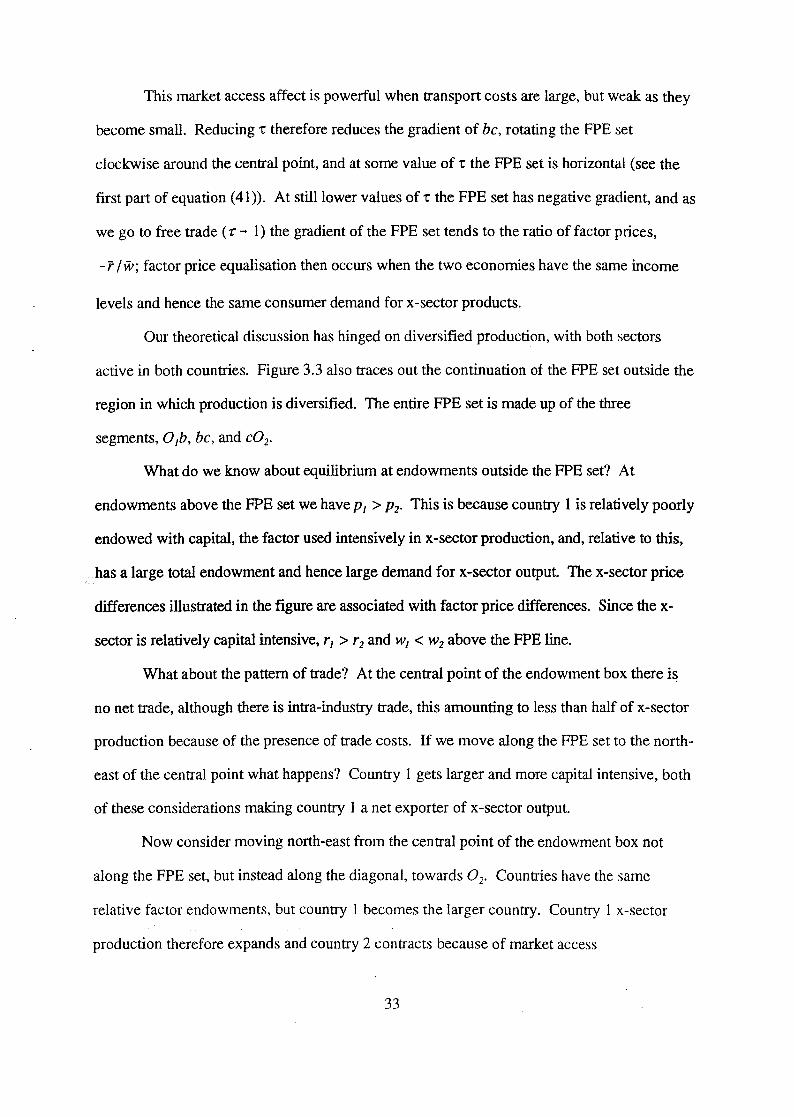
This market access affect is powerful when transport costs are large, but weak as they

become small. Reducing 1: therefore reduces the gradient of be, rotating the FPE set

clockwise around the central point, and at some value of 1: the FPE set is horizontal (see the

frrst part of equation (41». At stilllower values of 1: the FPE set has negative gradient, and as

we go to free trade ( 1:'" l) the gradient of the FPE set tends to the ratio of factor prices,

-r /w; factor price equalisation then occurs when the two econornies have the same income

levels and hence the same consumer demand for x-sector products.

Our theoretical discussion has hinged on diversified production, with both sectors

active in both countries. Figure 3.3 also traces out the continuation of the FPE set outside the

region in which production is diversified. The entire FPE set is made up of the three

segments, 0lb, be, and e02•

What do we know about equilibrium at endowments outside the FPE set'? At

endowments above the FPE set we have PI > P2' This is because country 1 is relatively poorly

endowed with capital, the factor used intensively in x-sector production, and, relative to this,

has a large total endowment and hence large demand for x-sector output The x-sector price

differences illustrated in the figure are associated with factor price differences. Since the x­

sector is relatively capital intensive"1 > '2 and WI < W2 above the FPE line.

What about the pattem of trade'? At the central point of the endowment box there i~

no net trade, although there is intra-industry trade, this amounting to less than half of x-sector

production because of the presence of trade costs. If we move along the FPE set to the north­

east of the central point what happens'? Country l gets larger and more capital intensive, both

of these considerations making country 1 a net exporter of x-sector output.

Now consider moving north-east from the central point of the endowment box not

along the FPE set, but instead along the diagonal, towards 02' Countries have the same

relative factor endowments, but country 1 becomes the larger country. Country 1 x-sector

production therefore expands and country 2 cont:racts because of market access

33

considerations. We therefore observe country 1 being a net exporter of x-sector output This

has the interesting implication that each country is a net exporter of the product which is

relatively intensive in its expensiye factor. Essentially, market access considerations are more

powerful than factor price differentials in determining location.

Moving along the 0 10 2 diagonal the two economies have the same relative factor

intensities, so market access considerations determine the pattern of trade. What happens as

we move away from the diagonal'? As we move far enough away so faetor market

considerations come to dominate, and the pattern of net trades reverts to that expected from

Heckscher-Ohlin theory. For example, at a point near the top of the fig. 3.2 and to the right of

centre, country 1 is large, but very labour abundant relative to country 2; it will then export z,

the labour intensive good.

This is all illustrated in figure 3.2. On the curved line there is intra-, but not inter­

industry trade. Below it country l is a next exporter of x-sector output, and above it a net

importer -- by virtue of either small size or relative labour abundance.

3f FaCtor prices.jactor mobility, and 'neweconomic geography'.

We have so far assumed that neither eapita! nor labour are intemationally mobile.

What happens if these faetors can mo ve in response to international factor price differences?

We have already seen how x-seetor produetion is drawn towards large economies for market

access reasons. But the locational attractiveness of large economies raises factor demands

and factor prices in these economies, so attracting factor inflow and making large economies

even larger. This suggests a 'positive feedback' or 'cumulative causation' mechanism, under

which factor mobility may be destabilising, eausing eeonomie activity to agglomerate in one

country. These forces were studied in Krugman (1991a,b). In this section we generalise

Krugman's analysis by placing it within the 2x2x2 framework we have developed.

So far, we have 100keC! at factor prices in terms of the numeraire. However, price

34

indices Si differ between countries, and so therefore does the cost of living, as measured by the

uni t expenditure functions, e( 1 ,s). We shalllook at cases where mobile factors consume in

the host economy, so incentives to move are determined by factor returns deflated by these

expenditure functions.

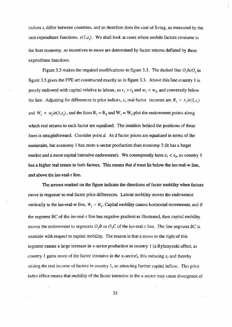
Figure 3.5 makes the required modifications to figure 3.3. The dashed line Ojbe02 in

figure 3.5 gives the FPE set constructed exactly as in figure 3.3. Above this line country 1 is

poorly endowed with capital relative to labour, so r l > r2 and wl < w2' and conversely below

the line. Adjusting for differences in price indices, Si' real factor incomes are R j = r/e(1,s)

and W j = w/e( 1 ,S j) , and the lines RI = R2 and W I = W 2 plot the endowment points along

which real returns to each factor are equalised. The intuition behind the positions of these

lines is straightforward. Consider point d. At d factor prices are equalised in terms of the

numeraire, but economy 1 has more x-sector production than economy 2 (it has alarger

market and a more capital intensive endowment). We consequently have sJ < S2' so country 1

has a higher real return to both factors. This means that d must lie below the iso-real-w line,

and above the iso-real-r line.

The arrows marked on the figure indicate the directions of factor mobility when factors

move in response to real factor price differences. Labour mobility moves the endowment

vertically to the iso-real-w line, Wt = WZ' Capital mobility causes horizontal movements, and if

the segment BC of the iso-real-r line has negative gradient as illustrated, then capital mobility

moves the endowment to segments ° jB or 02C of the iso-real-r line. The line segment BC is

unstable with respect to capital mobility. The reason is that a mo ve to the right of this

segment causes a large increase in x-sector producti~m in country l (a Rybczynski effect, as

country 1 gains more of the factor intensive in the x-sector), this reducing sJ and thereby

raising the real income of factors in country l, so attracting funher capital inflow. This price

index effect means that mobility of the factor intensive in the x-sector may cause divergence of

35

the structure of the two economies.

The comparison of labour and capital mobility indicates that divergence is associated

with mobility of capita!, the factor used intensively in the imperfectly competitive sector.

What if both capita! and labour are mobile? The only point in the figure at which real factor

price equalisation occurs at point E. This point is unstable -- a small perturbation around the

point leads to divergence. Full factor mobility therefore leads to one of the origins, with all

activity agglomerated in one of the locations.

The instability outlined above hinges on the line segment Be having negative gradient,

and this will be so if transport costs, -r, are not too large. To see this it is worth developing

the special case of this model originally put forward by Krugman (1991a). Krugman

specialises the model by assuming that each sector uses a single factor, so technology

coefficients take the form:

bw = 0, br = l, Cw = l, cr = O. (42)

The x-sector only uses capita!, and the z-sector only uses labour. (Krugman refers to the x­

sector as manufacturing, using manufacturing labour, and the z-sector as agriculture using

peasants who are distinct from manufacturing labourers. We retain our original, if less

colourful, terminology). Since the z-sector is numeraire, this assumption irnmediately fixes

wages,

(43)

With this structure it is easy to see that the factor market condition (equation (40), using (42)

and pricing equation (24» reduces to

(44)

Krugnian assumes that labour is immobile and capital is perfectly mobile in response to

36

differences in host country real returns5• This means that equilibrium returns satisfy

(45)

where o is the share of the x-sector in consumption, so the denorninators perform the role of

deflating by the local cost of living index.

We shall restrict analys is to the following question. Suppose that the x-sector is

concentrated in country I (n j > O. n2 = O). For what parameter values is this an equilibrium?

The assumption that n2 = O simplifies analysis greatly. First, it means that the price indices

(equations (19)) collapse down to

(46)

Second, it means that expenditure levels in each country reduce to

(47 )

where K is the world stock of capital and because country 2 has no x-sector production, it also

has no capita!. Furthermore, we shall assume that each country has half the world' s

endowment of labour, and write L1 = Lz = U2. Since capita! income equals x-sector output it

takes fraction o of world income, and labour income equals z-sector output it takes fraction 1

- o of income. The ratio of capital income to labour income must therefore equal the ratio of

expenditure shares of each good, so rlK/ L = 0/ (l-o). This means that expenditures can be

rewritten as,

El = OL(~), 2 1 - o

oL

2 (48)

Third, the assumption that 112 = O allows us to write the country l product market

condition (equation (30). using (46)) immediately as,

37

(49 )

We must now check whether our assumed pattern ofproduction, nI > O, n2 = O is an

equilibrium. It will be so if a potential entrant in country 1 would fail to make the level of

sales required for break even. The expression for break even is given above as equation (30),

so the condition is

(50)

where the left hand side gives the scale the potential entrant must reach to break even, and the

right hand side gives demand for its output Using equations (45) - (49) this simplifies to the

condition

(51)

Providing parameters satisfy this condition, agglomeration of activity is an equilibrium. The

relationship is illustrated, as a function of 't, on figure 3.6. At very high 't agglomeration is not

an equilibrium.6 This is because there is demand for x-sector output from the immobile factor,

labour, in both countries, and this has to be met by local production. At free trade, 't = 1, there

is nominal and real FPE over the entire diversification set However, there is a range of values

of 't at which the right hand side of (51) is less than unity, and at these points agglomeration of

activity in one location is an equilibrium.

This result is very extreme, and it is easy to think of considerations that would slow

down or halt agglomeration forces -- adjustment costs, or the existence of other immobile

factors (land). Nevertheless, the mechanism is important, and suggests that factor mobility

may have perverse effects, tending to make the distribution of economie activity unequal

between locations. This same mechanism has been used in the regional economics literature to

38

explain the development of urban centres (for example Fujita (1988». For discussion of

alternative forces with give rise to agglomeration see Krugman (1991 b).

4. Concluding comments:

These notes discuss some of the main results and models from the theory of

international trade under imperfeet competition. They are necessarily both selective and

superficiaI. Multinationals are conspicuous by their absence, and the reader is refelTed to

Markusen (1995) for a recent survey. Up to date and exhaustive treatments of other topics

are provided in volume III of the Handbook of International Economics, published in 1995.

(See references to Brander (1995), Baldwin and Venables (1995».

39

Appendix;

Simulations: Figures 3.1-3.5 were computed from simulations use the following functional

forms:

b(w.,r.) l l

1/2 e(1,s) = Sj •

W orId endowments are set at K = L = 1. The elasticity of demand for a single variety of

(52)

differentiated product, € = 5. National fum'i have flXed input requirement f = 0.25. Values of

1:' are reported in the text.

Endnotes:

1. Some aspects of this analysis are developed in Dixit (1984). Another valuable reference for the policy material is Brander (1995).

2. We index tax instruments by the finn on which they bear, not the govemment to which revenue accrues

3 . This function II embodies equilibrium behaviour, and is different from the profit functions of section 2c

4. The Cobb-Douglas assumption is necessary for the FPE set to be linear, but not for it be a one dimensional subset of the endowment space.

5. This means that income of the mobile factor is consumed in the host not the source country -- plausible if the mobile factor is some type of labour, but less plausible if it is capita!.

6. This is consistent with our discussion of the way in which changes in 1:' rotate the nominal FPE line (eg eqn (41» and hence determine the slope of the real FPE line of figure 3.5

40

References:

R. Baldwin and AJ. Venables, (1995), 'Regional econorruc integration', in Handbook o/

International Economics, vol III, ed G. Grossman and K. Rogoff, EIsevier,

Amsterdam.

S. Ben-Zvi and e. Helpman, 'Oligopoly in segmented markets', in G. Grossman (ed) Impetject

Competition and international trade' MIT, Cambridge MA.

J. Brander, (1995), 'Strategic trade policy', in Handbook o/ International Economics, vol III,

ed G. Grossman and K. Rogoff, EIsevier, Amsterdam.

J. Brander and P. Krugman (1983), 'A reciprocal dumping model of international trade',

Journal o/ International Economics, 15:313-323.

1. Brander and B. Spencer (1985), 'Export subsidies and market share rivalry' , Journal o/

International Economics, 18:83-100.

A. K. Dixit, (1984)'International trade policy for oligopolistic industries' Economic Journal,

94, 1-16.

A. K. Dixit and V. Norman (1980), The Theory o/ International Trade, Cambridge, CUP.

A. K. Dixit and J.E. Stiglitz (1977), 'Monopolistic competition and optimum product

diversity', American Economic Review, 67: 297-308.

1. Eaton and G. Grossman, (1986), 'Optimal trade and industrial policy under oligopoly',

Quarterly Journal o/ Economics, 10 l :383-406.

M. Fujita, (1988), 'A monopolistic model of spatial agglomeration', Regional Science and

urban economics, 12, 161-196.

E. Helpman and P.R. Krugman, (1985) Market Structure and Foreign Trade, Cambridge MA,

MIT press.

I. Horstman and J. Markusen, (l986),'Up the average cost curve; inefficient entry and the new

protectionism', Journal o/International Economics" 20, 225-247.

E. HelpInan and P.R. Krugman, (198'1) Policy, Cambridge MA, MIT press.

41

P. Krugman (1979), 'Increasing returns, monopolistic competition and international trade',

Journal of International Economics, 9: 469-479.

(1980), 'Scale economies, product differentiation and the pattern of trade', American

Economic Review, 70: 950-959.

(1981), 'Intra-industry specialisation and the gains from trade' , Journal of P oUtical

Economy, 89: 959-973.

(1991a), Increasing returns and economic geography', Quarterly Journal of

Economics

( 1991 b), Geography and Trade, MIT, Cambridge MA

J.R. Markusen (1981) 'Trade and the gains from trade with imperfect competition', Journal of

International Economics, 11: 531-551.

J .R. Markusen and AJ. Venables, (1988) 'Trade policy with increasing returns and imperfect

competition; contradictory results from competing assumptions, Journal of

International Economics, 24: 299-316.

A. Smith and A.J. Venables, (1988), 'Completing the internal market in the European

Community; some industry simulations', European Economic Review, 32, 1501-1525.

Spence, A.M., (l976),'Product selection, fIxed costs and monopolistic competition' Review

of Economic Studies. 43, 217-235.

AJ. Venables (1985), 'Trade and trade policy with imperfeet competition; the case of identical

products and free entry', Journal of International Economics, 19, 1-20.

AJ. Venables (1990), 'International capacity choke and national market games', Journal of

International Economics, 29, 23-42.

AJ. Venables (1994), 'Tariffs and subsidies with price competition and integrated markets',

Oxford Economic Papers, 46, 30-44.

42

/ /

/ /'

/'

/ /

/' /'

/ /

/ /

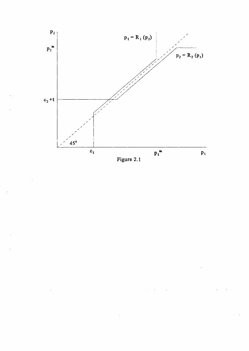
/ 45° /

el

/

/

/

/'

/

/' /

/

/

Figure 2.1

/ /

/

/

PI m

/ /

/'

/ /

/ ~----/

/

/

PI

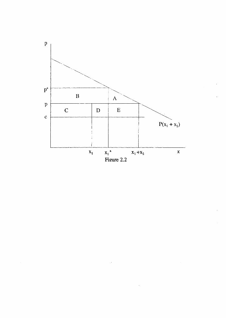
p

"-~

"

'~ ,

~, "

~-~,

'~

"-...

-~--

p

B A '~ ~

C D E c

Xta x

FiQUfe 2.2

p

'-.~

"-~ "~

~ r

B ~~ A ~

p C D E

c+ t G H

P(X1 + X2) F

c

+x Xl Xl a Xl 2 x

Filmre 2.3

PI

.... --.,

-----~ E --- ~

I PI

P. P2 19ure 2.4

P2

B c x - nI> O n > O ) 2 ,

x --

t

Figure 3.1: t = 1.0

ni / n2

I I

ntfn2 I

I

/ , /

/r /

/

I /

/ /

I / /

I /

/

I / /

I /

/ /

I l I

/ /

I / I

I /

/ / I

I / /

I / /

I /

/

I /

/ / I

J/ I //1 I

/

1 / /

/ 1 /

I I

/ / 1 l

't l - e 't e - l El / E2

Figure 3.2

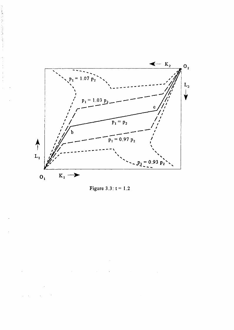
1~ ... : ... ~ __ ~_~_~_~~ ________________ ~~~~K~2~ __ ... ...... o ,'" 2

',PI = 1.07 P2 "", .." ' ..' ' : \ __________ -----;hj " PI = 1.03 P2 - -' ,,' ----- , , _---- l, ,r

" / c ~ " / /: " /, P, = P, /,' 11 b /,' ,n ---,I ----- ' ,/J _--- p-o ' ,/. r l - .97 P2 I

,0/ I~,~--------------\ \ , '/, .." ~ .." ~ ," ... '

~ ____ ~~~~ ________________ ~"'~"'~"'~Y.~1~=~O~.9~3~!~"~"'~~ ..... 2 '

0, K,~ - - '

t

Figure 3.3: t = 1.2

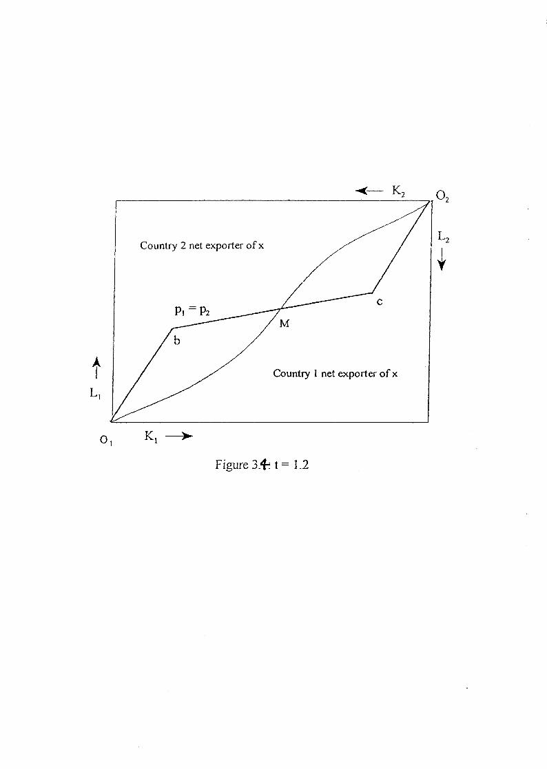
~- K2 o ~----------------------------------~------~< 2

Country 2 net exporter of x

t Country l net exporter ofx

K -~ 1

Figure 3.+. t = 1.2

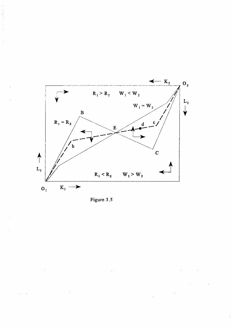
B

t

Figure 3.5

w 1 >w 2

~K 2

c

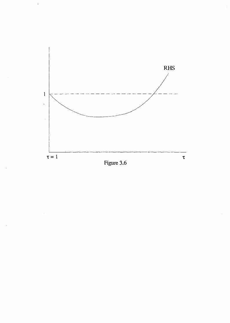
RHS

l

~~-----------------------_ .. -

't=1 Figure 3.6