Embed Size (px)
Citation preview

Supervisor: Evert Carlsson Master Degree Project No. 2015:81 Graduate School
Master Degree Project in Finance
The Inconvenient Truth of the Downside Beta
Mikael Ahlstedt and Jonatan Stål

The Inconvenient Truth of the Downside Beta
Mikael Ahlstedt Jonatan Stål
May 30, 2015
Abstract
In this thesis, we perform a robustness test of the interesting findings by
in particular Artavanis (2013), but also Ang et al. (2006) and others,
who find evidence that a downside beta outperforms the CAPM beta in
its ability to explain excess stock returns in a test developed by Fama
and French (1992). Stating that the CAPM beta is outperformed by the
less known downside beta is a bold statement, and could indicate that
information of a downside beta can be used to achieve abnormal excess
returns on the stock market. These findings deserve robustness tests to
either strengthen their case or show that the results are inconsistent across
different markets or time periods, which is the motivation for writing this
thesis. Our main findings show that there is no difference in the ability
of the CAPM beta and the downside beta to explain excess returns in a
Fama and French (1992) test during the years 2000-2014 on the Frank-
furt, London and Stockholm stock exchanges. Thus, the results of the
robustness test are demotivating, weakening the case for the downside
beta rather than accepting its superiority.
Acknowlegement
We would like to thank our supervisor Dr. Evert Carlsson for providing
valuable feedback and suggestions that improved our thesis.

Contents
1 Introduction 1
2 Literature Review 42.1 Return —variance trade-off in portfolio optimization . . . . . . . 4
2.2 The Capital Asset Pricing Model . . . . . . . . . . . . . . . . . . 5
2.3 Critique of the CAPM . . . . . . . . . . . . . . . . . . . . . . . . 6
2.4 Semi-variance and downside beta . . . . . . . . . . . . . . . . . . 7
3 Theory 113.1 Mean —variance and mean —semi-variance . . . . . . . . . . . . 11
3.2 Beta and downside beta . . . . . . . . . . . . . . . . . . . . . . . 13
3.3 Tests of the CAPM beta and the downside beta . . . . . . . . . . 13
4 Data and Methodology 164.1 Data sources and the dataset . . . . . . . . . . . . . . . . . . . . 16
4.2 The Fama-French test . . . . . . . . . . . . . . . . . . . . . . . . 16
4.2.1 The sorting process . . . . . . . . . . . . . . . . . . . . . . 17
4.2.2 Estimating the portfolio betas . . . . . . . . . . . . . . . . 17
4.2.3 The Fama-MacBeth regressions . . . . . . . . . . . . . . . 18
4.2.4 Criterions for answering the research question . . . . . . . 18
5 Results and Analysis 195.1 Summary statistics of the dataset and the portfolios . . . . . . . 19
5.2 The Fama-MacBeth regressions . . . . . . . . . . . . . . . . . . . 23
5.3 Analysis and discussion . . . . . . . . . . . . . . . . . . . . . . . 25
6 Conclusion 28
References 29
A Portfolio returns sorted on size and downside beta 30
B Portfolio returns sorted on BE/ME and CAPM beta 31
C Portfolio returns sorted on BE/ME and downside beta 32

1 Introduction
Portfolio optimization is an important part of financial theory, still to this day
heavily influenced by early financial theorists such as Harry Markowitz and
William Sharpe, amongst others. In a seminal article, Markowitz (1952) intro-
duces the portfolio selection problem as a two-stage process where the individual
seeks to maximize expected returns while minimizing the variance of returns.
Markowitz’s model is widely accepted within the literature, and was the founda-
tion for the famous Capital Asset Pricing Model (CAPM) developed by Sharpe
(1964), Lintner (1965) and Black (1972) (SLB). SLB show that the expected
return of any security can be compared to the risk free return and the expected
market return by means of the security’s beta value, where beta is the correla-
tion of a security’s excess return to the excess return achieved by the market
portfolio.
The beta value has had a large impact on financial theory and on the financial
industry. It is one of the key statistics used to present or describe a particular
stock (for example, Yahoo Finance presents 15 statistics of which beta is one,
in its stock overview).
By taking a step back, rather than accepting the popular mean —variance
and CAPM theories, and focusing on what an investor actually wants to achieve
with portfolio optimization, it is relevant to ask whether or not Markowitz
(1952/1959) was right in using the return —variance trade-off. The ultimate
aim for someone building an investment portfolio must be to optimize the return
relative to the risk. Markowitz (and subsequently SLB in the CAPM model)
used variance as the measure of risk, and this is where some see a weakness
of the model. Variance includes both gains and losses, and the models see
both large gains and large losses as equally bad. Why would an investor be
equally worried about large gains and large losses? In fact, Markowitz (1959)
proposes an alternative measure, called semi-variance, which only focuses on
downside variance as a measure of risk. Although pointing out several benefits
with semi-variance, Markowitz (1959) bases his theory on normal variance due
to its easier computation and it being more well-known than semi-variance.
However, research of portfolio optimization based on semi-variance did not end
with Markowitz (1959). Several authors have dwelled into the subject, among
the more well known, Hogan and Warren (1974) develop a downside beta value
based on semi-covariance.
1

The CAPM beta value has been criticized by Fama and French (1992), who
show that when one controls for firm size and book-to-market value of equity,
the beta value does not explain the excess returns on the US stock market in
the years 1963-1990. Several authors have since looked into other risk measures,
and in particular conditional beta and downside beta, which has been found to
better explain excess return than the CAPM beta, see for example Howton &
Peterson (1998), Ang et al. (2006), Pettengill, Sundaram & Mathur (2002) and
Artavanis (2013).
To either strengthen the validity of the downside beta or to weaken its case
against the CAPM beta, we perform a robustness test of the findings of Ar-
tavanis (2013) and Ang et al. (2006) who both use the US market in their
studies. We develop the research further by testing whether a downside beta
approach for estimating risk better explains excess return than the CAPM beta
on the Frankfurt, London and Stockholm stock exchanges in order to test if the
superiority of the downside beta is consistent across different markets.
To summarize, the thesis tests the following research question:
• Does a downside beta better explain excess returns than the CAPM beta
on the Swedish, German and Brittish stock markets?
We find no evidence that suggests that the (Hogan-Warren) downside beta out-
performs the CAPM beta in its ability to explain cross-sectional excess returns
in a Fama and French (1992) test on the Frankfurt, London and Stockholm
stock exchanges in the years 2000-2014. In the cross-sectional regressions, the
coeffi cients for the downside beta and the CAPM are similar in magnitude and
statistical significance, in no occasion is one statistically significant when the
other is not. Thus, the results of the robustness test are demotivating, weaken-
ing the case for the downside beta rather than accepting its superiority.
We also find that size is positively related to excess returns in Frankfurt and
Stockholm during the years 2000-2014, whereas the size effect is insignificant
in London. Conversely, the book-to-market value is positively related to excess
returns in London and Stockholm, but not in Frankfurt. The fact that the results
differ in the different markets is proof that the results of Fama and French (1992)
are not universal across markets. The analysis shows some weaknesses of the
test itself. In particular, the results are sensitive to the market performance in
the tested time period.
2

The remainder of this thesis is organized as follows: In order to familiarize
the reader with the subject, Chapter 2 presents the relevant literature sub-
sectioned in a chronological order, including the return —variance trade-off in
portfolio optimization, the capital asset pricing model, critique of the CAPM
and semi-variance and downside beta. Chapter 3 expands the theories presented
in Chapter 2 in a mathematical format. The data and the methodology are
discussed in Chapter 4. Chapter 5 presents and analyses the results obtained in
the study, and the thesis is concluded in Chapter 6.
3

2 Literature Review
This chapter summarizes relevant literature in order to set the frame for the
subsequent chapters of the thesis. The relevant literature has been divided into
four parts; Return —variance trade-off in portfolio optimization, The Capital
Asset Pricing Model, Critique of the CAPM and Semi-variance and downside
beta.
2.1 Return —variance trade-off in portfolio optimization
Markowitz (1952) defines the portfolio selection process in two steps, where in
a first step an investor forms his beliefs about future performance, and in the
second step chooses his portfolio based on those beliefs. How such beliefs are
formed is not thoroughly discussed by Markowitz (1952), who rather focuses on
the second step —that of portfolio selection.
The aim of portfolio optimization is to minimize the risk given an expected
level of return, or analogously maximize expected return given an expected level
of risk, which Markowitz (1952) defines as the variance in returns around its ex-
pected value. An effi cient portfolio is a portfolio in the attainable set (all possible
combinations of securities) such that the expected return cannot be increased
without increasing the expected variance, and the expected variance cannot be
decreased without decreasing the expected return. Figure 1 plots expected re-
turn versus expected variance, where the effi cient portfolios are the ones on the
border of the top left part of the attainable set (Markowitz, 1952/1959).
The rationale in Markowitz (1952/1959) for reducing risk when pooling sev-
eral securities in a portfolio is (perhaps self-evidently) that returns across secu-
rities are not perfectly correlated. That is, when one security increases in value,
another might decrease, which when aggregated into a portfolio decreases the to-
tal variance of the portfolio returns. However, since security returns are almost
always positively correlated, aggregating securities into a portfolio can never
completely eliminate the risk. The systematic risk will always be present even
in an optimized portfolio (Sharpe, 1964). Further, due to market limitations,
not even the idiosyncratic risk can be completely diversified away.
4

Figure 1: The return —variance trade-off. The attainable set of portfoliosdepicting the return — variance trade-off for investors choosing portfolios. Ifinvestors are rational, allowed to borrow at the risk free rate, rf , and agree onpreferences, favouring high returns and low variance, the market portfolio mustbe the tangency portfolio M. Based on the work by Markowitz (1952/1959),Sharpe (1964) and Lintner (1965).
In the final part of his book, Markowitz (1959) shows his analysis based on
semi-variance rather than variance. Semi-variance is defined as the variance
measured as the average of the squared negative deviations from the expected
returns only (more on this in a later chapter). Markowitz (1959) argues that
this approach focuses on reducing losses, rather than reducing pure volatility,
and even proceeds to state that:
“Analyses based on S [semi-variance] tend to produce better portfolios than
those based on V [variance]” (Markowitz, 1959)
However, among the downsides of using semi-variance are its larger com-
plexity, it being less well-known and its more demanding computing methods,
taking two to four times longer to perform on a “high speed electronic computer”
(Markowitz, 1959).
2.2 The Capital Asset Pricing Model
Markowitz (1952/1959) does not discuss in detail what particular portfolio in
the effi cient set an investor should choose. Sharpe (1964) and Lintner (1965)
use the model of Markowitz and add a risk free security and the assumption
that all investors agree on expected returns, variances and covariances. When an
5

investor can lend and borrow at the risk free rate, Sharpe (1964) shows that there
will only be one particular portfolio chosen by each and every investor. Given
that an investor has a utility function that increases in expected return and
decreases in expected variance, where both inputs have a marginally decreasing
effect on the utility, the optimum portfolio is the one in the effi cient set that is
tangent to a straight line between the effi cient set and the risk free rate, as seen
in Figure 1. This line is commonly referred to as the Capital Market Line. The
total risk level is adjusted by lending or borrowing at the risk free rate (Sharpe,
1964).
The portfolio called M in Figure 1 is shown by Lintner (1965) to be the
market portfolio. Since all investors agree on future prospects, they all invest
in portfolio M and adjust their level of risk by lending or borrowing at the risk
free rate. Thus in order to achieve market equilibrium, portfolio M must be the
market portfolio. The weights of each particular stock in the market portfolio
are the market values of each individual stock divided by the aggregate market
value of all stocks (Lintner, 1965).
Having defined the optimal portfolio choice, Sharpe (1964) shows that since
a portfolio is a linear combination of a number of securities, and that, in theory,
all non-systematic risk can be diversified away, the only risk that should be
considered for a particular stock is how it covaries with the market. That is, for
a relatively safe security, which is rather independent of the market performance,
an investor can accept a low expected return. On the other hand, for an investor
to accept a security that covaries strongly with the market, an investor requires a
large expected return. Although not using the word beta, Sharpe (1964) defines
the movement in relation to the effi cient portfolio as the correlation between the
returns of the security and the returns of the market, which has later become
the well-known CAPM beta.
2.3 Critique of the CAPM
Sharpe (1964), Lintner (1965) and Black (1972) concluded that stocks with a
high beta value should be rewarded with a large expected return, and that
no other risk measure should be necessary, a conclusion that has received cri-
tique from several academics since. Fama and MacBeth (1973) test the CAPM
model by regressing monthly returns on beta values, squared beta values and
the residuals from the market model, which in turn regresses individual excess
stock returns solely on the market excess return.
6

The dataset used by Fama and MacBeth (1973) stretches from 1926 to 1968
and contains approximately 700 stocks divided into 20 portfolios throughout the
period. The whole sample is needed to show a statistically significant positive
coeffi cient for the beta value. For shorter periods, such as five to ten years, the
coeffi cient for the beta value is generally not statistically significant.
From their results, Fama and MacBeth (1973) cannot reject the hypothesis
that a higher beta yields linearly higher expected returns. However, although
the results are not clear-cut, Fama and MacBeth (1973) show that the constant
term in the regressions is statistically significantly different from the risk free
rate, in contrast to what is predicted by the CAPM.
In a later and well-known test of the CAPM, Fama and French (1992) en-
hance the Fama-MacBeth regressions with additional explanatory variables, us-
ing US data from 1963 to 1990, which yields different results than was obtained
by Fama and MacBeth (1973). Fama and French (1992) argue that stocks of
different size (market value) have different betas. When controlling for mar-
ket value of equity (ME) as a proxy for size, book-to-market value of equity
(BE/ME), leverage and the earnings-to-price ratio (E/P ), Fama and French
(1992) find no statistical significance for the coeffi cient of the beta value in the
Fama-MacBeth regressions, and the authors state that:
“In a nutshell, market β seems to have no role in explaining the average
returns on NYSE, AMEX, and NASDAQ stocks for 1963-1990, while size and
book-to-market equity capture the cross-sectional variation in average stock re-
turns that is related to leverage and E/P”
2.4 Semi-variance and downside beta
As was already noted by Markowitz (1959), there might be other measures of
risk that are more appropriate for portfolio optimization than pure variance. In
particular, Markowitz (1959) suggested semi-variance as an alternative measure
of risk. Unlike unconditional variance, semi-variance considers only observations
below a certain threshold, normally; zero, the risk free rate or the expected
return of the market.
If the return distribution is symmetrical, the variance and the semi-variance
framework produce the same results. However, when the return distribution
is asymmetrical, especially shown for a lognormal distribution by Price et al.
(1982), the two frameworks diverge.
7

A downside beta risk measure based on semi-covariance is appealing be-
cause a security is not necessarily considered more risky by an investor when
performing extraordinarily well at the same time as the market, as the CAPM
beta based on covariance would have us believe. Nor does it consider poor se-
curity performance while the market is performing well risk reducing, as the
conventional beta does (Artavanis, 2013). Hence, downside beta only attributes
adverse outcomes as risk increasing. Even though an investor might consider
abnormal positive returns as risk increasing, he will put more emphasis on neg-
ative abnormal returns due to decreasing absolute risk aversion as shown by
Post and van Vliet (2004), and loss aversion (Artavanis, 2013). Figure 2 shows
how the CAPM beta (all four quadrants) and the Hogan-Warren downside beta
(the leftmost quadrants) are affected by different co-movements of the portfolio
returns and the market returns.
A(+)
C(+)
D()
B()
Rp
RM
Figure 2: Covariance and beta. The different quadrants show how theCAPM beta is affected by different observations of the relation between portfo-lio returns, Rp, and the market returns, Rm. In quadrant B and D, the portfoliocovaries negatively with the market, which decreases the CAPM beta and thusthe perceived risk of the portfolio decreases. In quadrants A and C, the portfo-lio covaries with the market and the CAPM beta increases. The fact that theCAPM risk measure increases (decreases) in quadrant A (D) is unintuitive as in-vestors generally prefer profits over losses regardless of the market performance.The Hogan-Warren downside beta, based on semi-covariance, ignores outcomeswhen the market return is positive and is thus alleviated from the unintuitivequadrants A and D.
8

Over the years, a few different versions of downside beta have emerged.
Hogan and Warren (1974) use the risk free rate of return (which can be seen
as an opportunity cost of capital) as the threshold when they show that semi-
variance can replace variance to measure portfolio risk without losing the fun-
damental structure of the CAPM. In this setting, the effi cient portfolios are
those that minimize the semi-variance given the expected return, and the only
risk that rewards higher expected return is the co-movement with the market
when the market performs below the threshold (Hogan and Warren, 1974). The
corresponding downside beta is known as the Hogan-Warren downside beta.
Estrada (2002) presents a different version of the downside beta, where the
numerator is given by the covariance of the security return and the market
return conditional on both the security and the market performing below their
expected returns. A reason for this specification is to avoid the inconvenience
of an asymmetrical semi-covariance matrix that for example the Hogan-Warren
approach produces (Artavanis, 2013).
In a framework similar to that of Hogan andWarren (1974), Ang et al. (2006)
build their model on a representative agent with a “rational disappointment
aversion utility function”. In the framework of Ang et al. (2006), an investor
would be disappointed if he does not get at least his certainty equivalent (the
risk free rate of return) back from an investment. In addition, the authors
condition the semi-covariance on the market performing worse than its average
excess return.
In his treatise on downside risk, Artavanis (2013) methodologically examines
and compares the different recipes of downside beta with each other and the
CAPM beta. Artavanis (2013) finds that the Hogan-Warren beta is the only
specification that is consistent with the CAPM framework and state-preference
theory.
In Estrada’s (2002) framework, all risk reducing observations when the mar-
ket underperforms while the security outperforms the threshold are excluded
from the sample. Thus, the framework systematically overestimates the down-
side risk and it additionally strips the available dataset of observations resulting
in increased estimation errors (Artavanis, 2013).
The inclusion of two separate thresholds for the estimation of semi-covariance
in the framework of Ang et al. (2006) is shown by Artavanis (2013) to violate
state-preference theory. In particular, the problem arises from what he describes
as a “region-sign bias”, where in marginally bad states the return of the security
has the opposite effect on the risk premium than what would seem logical.
9

After having theoretically presented why the Hogan-Warren beta is prefer-
able, Artavanis (2013) also presents empirical evidence of its superiority contra
both its semi-covariant challengers and the CAPM beta by the use of Fama-
MacBeth regressions on US data from 1926 to 2010.
Howton and Peterson (1998) perform a Fama and French (1992) test on
US data from 1977 to 1993 on both the CAPM beta and a dual-beta model
developed by Bhardwaj and Brooks (1993). Howton and Peterson (1998) divide
the sample into two sub-samples; up markets and down markets. Up markets are
defined as months when the market return is higher than the median market
return, and down markets are defined as months when the market return is
lower than the median market return. Howton and Peterson (1998) find that
a beta value calculated during months with market returns below the average
market return is statistically significantly negatively related to excess returns
in bear markets, whereas the opposite holds in bull markets for beta values
calculated in months with market excess returns above their average. Pettengil,
Sundaram and Mathur (2002) perform a similar test to Howton and Peterson
(1998), although dividing the sample into sub-samples according to; up markets
— when the monthly market return minus the US one-month treasury bill is
larger than zero, and down markets —when the monthly market return minus
the US one-month treasury bill is smaller than zero. PSM (2002) find that the
CAPM beta is not statistically significantly related to excess returns across the
entire sample period. In accordance with Howton and Peterson (1998), PSM
(2002) find that when the sample is divided into sub-samples, bear (bull) beta
is statistically significantly negatively (positively) related to excess returns in
down (up) markets. However, in the same sub-samples, the CAPM beta is even
more significant. Thus, PSM (2002) come to the conclusion that sub-sampling
is suffi cient for beta to become significantly related to excess returns.
10

3 Theory
This chapter presents the theories discussed in Chapter 2 in a mathematical
format.
3.1 Mean —variance and mean —semi-variance
An effi cient portfolio is one that minimizes the expected variance, given the
expected return. Markowitz (1959) presents a general example with n securities.
The expected return of a portfolio is defined as
E =
n∑i=1
Xiµi (1)
where µi is the expected return of security i and Xi is the relative amount
invested in security i, such that
n∑i=1
Xi = 1 (2)
and
Xi ≥ 0 ∀ i (3)
which ensures no short-selling. The expected variance of a portfolio is therefore
V =
n∑i=1
n∑j=1
XiXjσij (4)
where σij is the covariance of the returns of security i and security j.
The problem of determining the effi cient frontier is then to maximize ex-
pected return∑ni=1Xiµi given the expected variance V =
∑ni=1
∑nj=1XiXjσij ,
or likewise minimize expected variance given the expected return. This can be
achieved by a number of programming techniques, for example a linear pro-
gramming model or Monte Carlo techniques (Markowitz, 1959). The resulting
effi cient frontier can then be plotted in the return —variance space as in Figure
1 above.
11

When analyzing a mean — semi-variance effi cient frontier, Equations (1)-
(3) are used as defined above, although Equation (4) needs to be rewritten.
Markowitz (1959) defines
r− =
{r if r ≤ 0
0 if r > 0(5)
where r is returns. A portfolio’s semi-variance is then defined as
So =∑i
∑j
sij (t1, ..., tk)XiXj (6)
where the semi-covariance between security i and j is calculated by
sij (t1, ..., tk) =1
T
K∑k=1
ritkrjtk (7)
where the index t represents time period (year, month etc.), T is the total
number of time periods studied and K is the number of time periods where the
market has negative returns.
Markowitz (1959) shows the rationale for using semi-variance rather than
variance by a discussion of distributions. Consider the two distributions of
returns in Figure 3 below.
xx x x x
4 % 3% 2 % 1 % 1 % 2 % 3 % 4 %
xx x x x
4 % 3 % 2 % 1 % 1 % 2 % 3 % 4 %
A
B
Figure 3: Distribution, variance and semi-variance. The variance of theobservations (denoted by x in the figure) is the same for both distribution Aand its reflection B, whereas the downside semi-variance is larger in distributionB as it is negatively skewed due to the larger outlier. Thus, an investor whobases his portfolio decision on variance would be indifferent between the twoportfolios, whereas if he uses semi-variance he would prefer portfolio A.
12

The variance of distribution A is the same as that of distribution B, whereas
the semi-variance is larger for distribution B than for distribution A. A mean
—variance analysis considers the two cases equally desirable, whereas a semi-
variance analysis would favor distribution A. In short, an analysis based on semi-
variance choses the distribution most skewed to the right (positively skewed) for
each given expected return.
3.2 Beta and downside beta
The classical CAPM equation developed by Sharpe (1964), Lintner (1965) and
Black (1972) is defined as
E (Ri) = Rf + βi [E (Rm −Rf )] (8)
where index i represents security i, index f represents the risk free asset and
index m represents the market portfolio. In Equation 8, βi is defined as
βi =cov (Ri, Rm)
var (Rm)(9)
There are several definitions of downside beta, an early version is the Hogan-
Warren downside beta developed by Hogan and Warren (1974), which according
to Artavanis (2013) is the only specification consistent with the framework pre-
scribed by Markowitz (1959) and state-preference theory. The Hogan-Warren
equivalent to Equation 9 is
β−i =cov ((Ri −Rf ) ·min (Rm −Rf , 0))
var (min (Rm −Rf , 0))(10)
3.3 Tests of the CAPM beta and the downside beta
Fama and MacBeth (1973) regress monthly portfolio returns on portfolio beta
values (expressed as the average of the betas of the individual securities in each
portfolio), the average of the squared security beta values for each portfolio
and the average of the standard error of the residuals in each market model
regression for each portfolio. Fama and MacBeth (1973) use the market model
Ri,t = αi + βiRm,t + εi,t (11)
13

where Rm,t is the excess market return in period t, Ri,t is the excess return of
security i in period t and εi,t is the residual of the regression in period t. Since
βi = cov(Ri,Rm)var(Rm)
and by construction cov (εi, Rm) = 0, then
var (Ri) = β2i var (Rm) + var (εi,t) + 2βicov (Rm, εi,t) (12)
i.e, from Equation 12, var (εi,t) is the only factor determining the distribution
of the returns that is not related to beta for security i.
The Fama-MacBeth regressions in their full form are then defined as
Rpt = γ̂0t + γ̂1tβ̂p,t−1 + γ̂2tβ̂2
p,t−1 + γ̂3ts̄p,t−1 (ε̂i) + η̂p,t (13)
where β̂p,t−1 is the average of the betas in portfolio p derived from Equation 11
in period t−1 and s̄p,t−1 (ε̂i) is the standard error of the residuals also obtained
from Equation 11. Fama and MacBeth (1973) find that the coeffi cients for
β̂2
p,t−1 and s̄p,t−1 (ε̂i) are insignificantly different from zero.
The test statistic used to test the significance of the coeffi cients of regression
13 in Fama and MacBeth (1973) is
t(¯̂γj)
=¯̂γj
s(γ̂j)√n
(14)
where n is the number of months in the test period.
Fama and French (1992) build on the research of Fama and MacBeth (1973)
by adding additional explanatory variables to the Fama-MacBeth regressions.
Market value of equity, book-to-market value of equity, leverage and the earnings-
to-price ratio are all included as additional risk factors. To distinguish between
the effects of size and beta in average returns, Fama and French (1992) adopt
a double sorting procedure by first sorting the securities according to size, and
then, within each size category, an additional sorting on pre-ranking betas for
the individual stocks. Thus, Fama and French (1992) use a similar sorting pro-
cedure as Fama and MacBeth (1973) with the addition of the initial sorting on
size (ME). The average betas within each size —beta sorted portfolio are then
given to each individual security within the particular portfolio in order to avoid
imprecise beta estimates for individual securities. These beta values are used
along with security specific data on ME, BE/ME, E/P and leverage in cross-
security regressions. Portfolios are updated yearly, as well as ME, BE/ME,
14

leverage and E/P for each security. The beta values and the natural logarithms
of the other explanatory variables are then regressed on the next twelve monthly
returns for each security. The process is repeated for each year, and time-series
averages of each cross-sectional coeffi cient are calculated along with t-statistics
according to Equation 14 (Fama and French, 1992).
Fama and French (1992) find that the coeffi cient for beta is not statistically
significant, with a t-statistic of only -0.46. Further, they find that the coeffi cients
for log(ME) and log (BE/ME) are significantly different from zero and that
these variables combined absorb the explanatory power of leverage and E/P .
Thus, Fama and French (1992) find no evidence that supports using the
CAPMmodel to explain excess returns in cross-sections. Artavanis (2013) shows
that when performing the Fama-MacBeth regressions on downside beta instead
of the CAPM beta, the downside beta remains statistically significant even in
Fama and French (1992) regressions.
15

4 Data and Methodology
This chapter presents the data sources and the specific data, as well as the econo-
metric techniques used to answer the research question in Chapter 1. Although
this chapter only describes the process of sorting on size and beta, sorting has
also been performed equivalently on the BE/ME and beta.
4.1 Data sources and the dataset
We use Bloomberg to obtain the monthly returns adjusted for dividends and
all other corporate actions, the market value of equity (ME) and the book-to-
market value (BE/ME) for all traded stocks included in the all-share indices
on the Frankfurt, London and Stockholm stock exchanges from 1995 to 2014.
Securities with missing data throughout the entire time period of either ME,
BE/ME or returns are excluded from the data set. Further, securities with
recordings of negative book values are also excluded from the data set, as in
Fama and French (1992), the number of such securities is small. Only the
most frequently traded security of each company is included in the data set, i.e.
usually shares of class B. The risk free rates are the one-month interbank rates
for the respective markets, also obtained from Bloomberg.
4.2 The Fama-French test
For the three markets specified above, we test if the CAPM beta and the Hogan-
Warren downside beta explain cross-sectional excess returns in the presence of
the logarithm of the market value of equity and the logarithm of the book-to-
market ratio. Based on the results of Fama and French (1992), we do not include
the earnings-to-price ratio or the leverage. The cross-sectional regressions in
their full form are specified as
Ri,t = γ̂0t + γ̂1tβ̂p + γ̂2t ln (MEi,Dec) + γ̂3t ln (BE/MEi,Dec) + εt (15)
where Dec refers to that the explanatory variables are taken from December in
the year before the returns (the dependent variable) were observed. The cross-
sectional regressions are performed monthly over the entire time period, except
for the first five years that are used for pre-ranking security betas. A detailed
description of the process follows below.
16

4.2.1 The sorting process
For each year, after an initial security beta pre-ranking period of five years,
the different securities are first sorted into septiles depending on their market
capitalization in December of the previous year. Since the number of securities is
not usually divisible by the number of size sorted portfolios, the largest and the
smallest size portfolios receive one extra security. Fama and French (1992) use
fixed market capitalization limits to sort into size sorted portfolios rather than
using our approach of assigning an equal number of stocks into each portfolio.
The size sorting approach by Fama and French (1992) yields too few securities
in some of the size sorted portfolios, which prevents further beta sorting and is
thus not used in our analysis. This difference in sorting methodology is unlikely
to affect the outcome of the analysis. Security betas are calculated from a
pre-ranking period of 60 months, using Equation 9. Within each size sorted
portfolio, a sorting of the pre-ranking betas is performed. The same method of
dealing with indivisibility as when sorting on size is applied to the beta sorting.
In order for a security to be included in this sorting, it must have data on
market value for December of the year in which the pre-ranking of the beta
values ends and monthly returns for the pre-ranking period and the following
twelve months. By performing this check yearly, we avoid any survivorship bias
from the easier solution to only analyze securities with data for the full sample
period.
4.2.2 Estimating the portfolio betas
The equal weighted monthly excess returns are calculated for each portfolio and
month in the data set after the initial pre-ranking period. The post-ranking
portfolio excess returns are regressed across the entire data set, using the market
excess return for each month and its first lag as explanatory variables.
Rp,t = θ0 + θ1RM,t + θ2RM,t−1 + εt (16)
The market return at time t for each market is defined as the value weighted
returns of the securities in the data set without missing data on either returns
or market capitalization at time t. The CAPM portfolio beta is calculated,
identically to the specification in Fama and French (1992), as the sum of the
slopes of the regression coeffi cients for the market excess return, θ1, and the
17

coeffi cient of its first lag, θ2. For Downside beta, Equation 10 is used to define
the post-ranking portfolio downside betas.
4.2.3 The Fama-MacBeth regressions
Fama-MacBeth regressions specified according to Equation 15 are performed for
each month of the dataset after the initial pre-ranking period. For each year,
securities are sorted into portfolios as was described in chapter 4.2.1 and are then
assigned the post-ranking beta of the portfolio to which they are assigned. By
re-sorting the portfolios yearly, a security can move across portfolios depending
on changes in its pre-ranking beta and its size. This allows some variation in
security beta while avoiding the estimation errors that follow from using security
betas directly (Fama and MacBeth, 1973; Fama and French, 1992). The cross-
sectional Fama-MacBeth regressions are run for all securities with suffi cient data
for each month, using security specific values of ME and BE/ME, for which
there is no error in the estimates. By rolling the regressions monthly, a total
of 180 regressions per market are performed with an average of 344 securities
per regression. The Fama-MacBeth coeffi cients are calculated as the time-series
averages of the cross-sectional regressions, and the standard errors are calculated
as in Equation 14.
4.2.4 Criterions for answering the research question
The results of the Fama-MacBeth regressions are presented in tables, and the
sign of the coeffi cients as well as their t-statistics are compared to the results of
Fama and French (1992), Artavanis (2013) and Ang et al. (2006). Although the
main purpose of the thesis is to test whether a downside beta better explains
excess returns than the CAPM beta, the fact that a Fama and French (1992)
analysis is performed on three different markets also allows the thesis to test
the robustness of the resluts obtained by Fama and French (1992).
In short, if the coeffi cient for downside beta consistently has a larger t-
statistic than the coeffi cient for the CAPM beta in the cross-sectional regressions
including the additional risk factors log(ME) and log(BE/ME), the downside
beta is deemed to better explain excess returns than the CAPM beta. Further, if
the results of the analysis are similar to the results of Fama and French (1992) in
the different markets, the Fama and French (1992) results are considered robust
across markets and different time periods.
18
5 Results and Analysis
This chapter first presents summary statistics of the data. Thereafter, the
results of the Fama-MacBeth regressions are presented and analyzed.
5.1 Summary statistics of the dataset and the portfolios
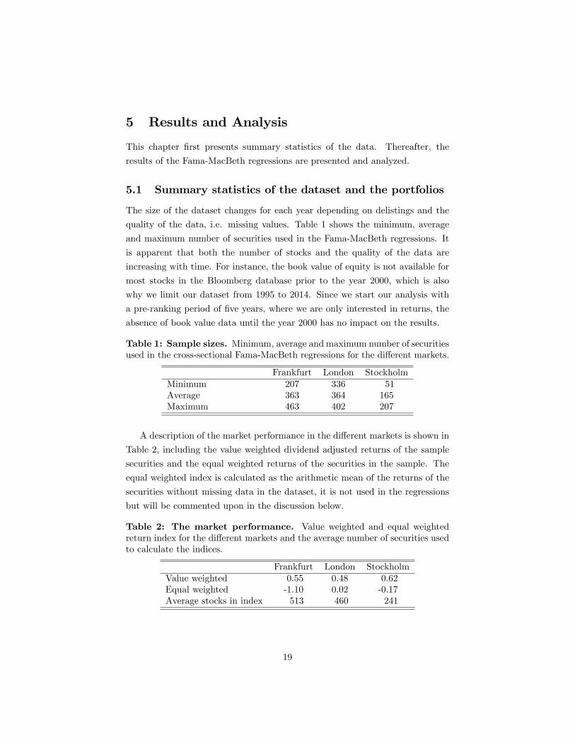
The size of the dataset changes for each year depending on delistings and the
quality of the data, i.e. missing values. Table 1 shows the minimum, average
and maximum number of securities used in the Fama-MacBeth regressions. It
is apparent that both the number of stocks and the quality of the data are
increasing with time. For instance, the book value of equity is not available for
most stocks in the Bloomberg database prior to the year 2000, which is also
why we limit our dataset from 1995 to 2014. Since we start our analysis with
a pre-ranking period of five years, where we are only interested in returns, the
absence of book value data until the year 2000 has no impact on the results.
Table 1: Sample sizes. Minimum, average and maximum number of securitiesused in the cross-sectional Fama-MacBeth regressions for the different markets.
Frankfurt London StockholmMinimum 207 336 51Average 363 364 165Maximum 463 402 207
A description of the market performance in the different markets is shown in
Table 2, including the value weighted dividend adjusted returns of the sample
securities and the equal weighted returns of the securities in the sample. The
equal weighted index is calculated as the arithmetic mean of the returns of the
securities without missing data in the dataset, it is not used in the regressions
but will be commented upon in the discussion below.
Table 2: The market performance. Value weighted and equal weightedreturn index for the different markets and the average number of securities usedto calculate the indices.
Frankfurt London StockholmValue weighted 0.55 0.48 0.62Equal weighted -1.10 0.02 -0.17Average stocks in index 513 460 241
19

The size and beta sorted portfolios’ average excess returns for the entire
sample period excluding the initial pre-ranking period are presented in Table 3,
Table 4 and Table 5 for the Frankfurt, London and Stockholm stock exchanges,
respectively. The smallest stocks with the lowest betas are found in the North-
west corner and the largest stocks with the highest betas are in the Southeast
corner, this logic applies to all tables in the remainder of this sub-chapter.
Table 3: Portfolio returns —Frankfurt. Monthly returns in percent forequal weighted double sorted portfolios sorted on size and pre-ranking betas.
Low β1 β2 β3 β4 β5 β6 High β7Small ME1 -1.00 -0.46 -1.36 -1.49 -1.27 -1.75 -3.59
ME2 -1.26 -1.39 -0.30 -0.57 -0.52 -0.50 -2.00ME3 -0.15 -0.42 0.56 0.02 -0.44 0.53 -0.07ME4 -0.16 -0.45 -0.23 0.45 -0.39 0.57 -0.78ME5 0.12 -0.13 0.25 0.45 0.83 0.52 -1.54ME6 0.39 0.51 0.73 0.47 -0.19 0.50 -0.48
Large ME7 0.31 0.11 0.61 0.06 -0.37 -0.09 0.04
Table 4: Portfolio returns —London. Monthly returns in percent for equalweighted double sorted portfolios sorted on size and pre-ranking betas.
Low β1 β2 β3 β4 β5 β6 High β7Small ME1 0.15 0.36 0.78 0.44 -0.02 0.26 0.37
ME2 0.54 0.50 0.36 0.01 -0.35 -0.79 -0.14ME3 0.38 0.13 -0.14 -0.16 0.14 -0.50 -0.43ME4 -0.14 0.19 0.36 0.73 0.03 -0.29 0.06ME5 0.15 0.13 0.22 0.39 -0.20 0.02 -0.48ME6 0.22 0.14 0.84 0.17 -0.14 -0.16 0.12
Large ME7 0.42 0.66 -0.11 -0.23 -0.21 0.20 0.06
Table 5: Portfolio returns —Stockholm. Monthly returns in percent forequal weighted double sorted portfolios sorted on size and pre-ranking betas.
Low β1 β2 β3 β4 β5 β6 High β7Small ME1 -0.18 0.13 1.15 -0.33 0.57 -0.87 -2.41
ME2 0.81 1.01 0.40 -0.16 -0.45 -1.01 -1.18ME3 -0.16 -0.26 1.02 -0.31 0.69 -0.11 0.37ME4 0.74 -0.11 0.63 -1.09 -0.78 -1.69 -0.92ME5 1.00 1.26 -0.05 0.87 0.18 -0.61 1.06ME6 1.12 1.07 0.38 0.59 1.08 0.68 -0.33
Large ME7 0.07 0.46 0.62 0.32 0.71 0.24 0.03
20

As can be seen from Table 3 and Table 5, there seems to be a positive
relation between size and excess returns in Sweden and Germany, while Table 4
shows the opposite relationship for the UK. The relationship between beta and
excess returns is not as easily seen in the tables, although a larger beta certainly
does not seem to be correlated with higher returns, as was found by Fama and
French (1992). When comparing Table 3-5 to the equivalent table by Fama and
French (1992) for stocks on the NYSE, AMEX and Nasdaq in the time period
of 1963 to 1990, there is a striking difference in the clarity of the patterns. The
table in Fama and French (1992) shows a perfect pattern of increasing returns
for decreasing size, whereas the existence of such a pattern is hard to see at a
first glance in our tables describing Frankfurt and Stockholm, and the opposite
relation seems to hold for London. Both in Fama and French (1992) and in our
study, the relationship between beta and returns is not obvious from looking at
the tables above.
Table 6-8 presents the portfolio betas of the size pre-ranking beta sorted
portfolios. In general, the portfolio betas increase with pre-ranking beta, which
indicates a rather good persistency in the beta values. In the equivalent table of
Fama and French (1992), the pattern with regard to pre-ranking betas is similar
to ours. Further, Fama and French (1992) find an almost uncanny pattern of
decreasing beta with increasing size. In fact, this pattern is much clearer than
the pattern we find between pre-ranking beta and post-ranking portfolio beta.
In comparison to the size —beta pattern observed in Fama and French (1992),
our results resemble a random walk.
For the London stock exchange it is hard to identify any pattern at all, but
it seems like the medium sized firms are the ones with the highest betas. In
both London and Frankfurt, the range of the beta values increases with firm
size, where the low betas tend to get lower and the high betas grow higher. The
range effect is not observed in Stockholm.
The beta values, in general, are lower in Frankfurt than in the other observed
markets, while London clearly has the highest values. Size-wise, the data for
the Stockholm stock exchange is most similar to the results in Fama and French
(1992). Interestingly, almost all beta values in Frankfurt are below one (average
0.72), whereas almost all are above one in London (average 1.34). This is
explained by the bottom row of the two tables, where the very largest firms
have low (high) betas in London (Frankfurt) and thus have a larger impact on a
value-weighted index and therefore balance the equation. In Stockholm, the beta
values are more balanced (average 0.93). However, it should be noted that the
21

average portfolio beta values mentioned above are calculated as the arithmetic
mean of the portfolio betas. If value weighted betas are used instead, the average
betas in Frankfurt are 1.10, in London 1.14 and in Stockholm 1.02. One would
expect the value weighted average of the betas to equal one. The observed
discrepancy is explained by the fact that the stocks used in the regressions are
not exact replicas of the stocks used to construct the indices, due to missing
data.
Table 6: Portfolio betas —Frankfurt. Estimated betas for equal weighteddouble sorted portfolios sorted on size and pre-ranking betas.
Low β1 β2 β3 β4 β5 β6 High β7Small ME1 0.37 0.51 0.59 0.90 0.69 0.65 0.31
ME2 0.42 0.44 0.53 0.53 0.61 0.85 0.76ME3 0.30 0.54 0.75 0.62 0.63 0.85 0.75ME4 0.44 0.46 0.64 0.51 0.62 0.77 1.22ME5 0.30 0.46 0.58 0.66 0.83 0.89 1.31ME6 0.25 0.42 0.61 0.80 0.91 1.16 1.41
Large ME7 0.46 0.72 0.70 1.09 1.30 1.47 1.51
Table 7: Portfolio betas —London. Estimated betas for equal weighteddouble sorted portfolios sorted on size and pre-ranking betas.
Low β1 β2 β3 β4 β5 β6 High β7Small ME1 1.11 1.18 1.44 1.12 1.47 1.58 1.74
ME2 1.03 1.02 1.40 1.47 1.51 1.75 1.83ME3 0.93 0.90 1.45 1.26 1.37 1.67 2.10ME4 0.90 1.09 1.23 1.47 1.57 1.49 2.02ME5 1.27 0.96 1.24 1.43 1.45 1.65 2.02ME6 0.58 1.06 1.03 1.32 1.41 1.75 1.95
Large ME7 0.53 0.66 0.72 1.18 1.38 1.49 1.64
Table 8: Portfolio betas —Stockholm. Estimated betas for equal weighteddouble sorted portfolios sorted on size and pre-ranking betas.
Low β1 β2 β3 β4 β5 β6 High β7Small ME1 0.67 0.78 0.88 0.78 0.60 1.14 1.38
ME2 0.62 0.67 0.77 0.56 0.70 1.12 1.00ME3 0.77 0.57 0.79 1.03 0.97 1.18 1.46ME4 0.63 0.75 0.83 0.91 1.10 1.42 1.65ME5 0.63 0.73 0.80 0.82 0.89 1.27 1.52ME6 0.60 0.69 0.80 0.76 0.88 0.97 1.18
Large ME7 0.79 0.90 0.98 0.86 1.03 1.08 1.55
22

The equivalents of Table 3-5 sorted on ME and downside beta, BE/ME
and CAPM beta and BE/ME and downside beta are found in Appendix A,
Appendix B and Appendix C, respectively. These tables show similar, but less
obvious patterns than the size and pre-ranking CAPM beta sorted portfolios.
5.2 The Fama-MacBeth regressions
The averages of the coeffi cients in the monthly Fama-MacBeth regressions, along
with their t-statistics according to Equation 14, are presented in Table 9. In
line with Fama and French (1992), the regressions generate negative coeffi cients
for the betas, both for the CAPM betas and the Hogan-Warren downside betas.
About half of our results, show that the coeffi cients for the betas are statistically
significant at the 5 % level, whereas Fama and French (1992) do not find any
significance.
When regressing excess returns on beta and log (ME) alone, we find that a
stock on the Frankfurt stock exchange is rewarded with 0.23 % larger monthly
excess returns when log (ME) is increased by one. A slightly lower effect is
seen in Stockholm (0.16 %), whereas in London an increase in log (ME) by one
decreases excess monthly returns by 0.04 %, although not statistically signifi-
cant. Thus, as was expected from observing Table 3, Table 4 and Table 5, the
effect of size is different in the different markets, and the results in Stockholm
and Frankfurt are opposites to those found by Fama and French (1992). The
book-to-market ratio has no significant effect on the excess returns in Frankfurt,
whereas in Stockholm and London the log (BE/ME) coeffi cient is positive and
statistically significant at the 5 % level, yielding an additional 0.4 % to 0.5 %
excess return per month and unit. When using the downside beta in the regres-
sions rather than the CAPM beta, the results change somewhat, although the
signs of all coeffi cients remain the same.
When running the Fama-MacBeth regressions including both log (ME) and
log (BE/ME), the results differ strongly between the different markets. The
coeffi cients for both the CAPM beta and the downside beta are statistically
insignificant in Frankfurt and London, which is in line with the results of Fama
and French (1992). However the coeffi cients of both the CAPM beta and the
downside beta in Stockholm are negative and statistically significant at the 5 %
level.
The differences in the statistical significance of the CAPM betas and the
downside betas are negligible and, for instance, in London the downside be-
23

Table 9: Results of the Fama-MacBeth regressions. After a beta pre-ranking period of five years, a total of 180 cross-sectional regressions, one foreach month in 2000-2014 are run, and then the time-series averages of the co-effi cients.The t-statistics are calculated according to equation 14 and presentedin the parenthesis. The cross-sectional regressions are run on 49 size-beta dou-ble sorted portfolios. The portfolios are re-sorted yearly, which allows variationin beta-estimates of the individual securities. Data for market value of equityand book-to-market value is taken at the firm specific level. The regressioncoeffi cients are expressed in percent.
β β− log (ME) log (BE/ME)Frankfurt -0.64 (-1.36) 0.23 (3.56)
-0.11 (-0.23) -0.29 (-1.87)-0.60 (-1.26) 0.25 (5.25) -0.01 (-0.04)
-0.43 (-1.21) 0.24 (3.63)-0.17 (-0.47) -0.31 (-2.02)-0.43 (-1.19) 0.26 (5.25) 0.02 (0.12)
London -0.46 (-1.36) -0.04 (-0.75)-0.80 (-2.38) 0.52 (3.44)-0.50 (-1.61) 0.01 (0.20) 0.33 (2.24)
-0.43 (-1.45) -0.01 (-0.12)-0.68 (-2.38) 0.40 (2.68)-0.47 (-1.72) 0.05 (0.90) 0.35 (2.33)
Stockholm -2.27 (-3.39) 0.16 (2.57)-1.87 (-2.49) 0.42 (2.67)-1.70 (-2.58) 0.19 (2.71) 0.52 (2.98)
-1.33 (-2.66) 0.20 (3.03)-1.20 (-2.33) 0.39 (2.42)-1.16 (-2.58) 0.25 (3.28) 0.59 (3.20)
tas are on average slightly more significant than the CAPM betas, whereas
the opposite holds for Frankfurt and Stockholm. The fact that there hardly
is any difference between the two beta measures is a strong contradiction to
the findings of Artavanis (2013), who finds that the CAPM beta is statistically
insignificant in the presence of log (ME) and log (BE/ME), whereas the down-
side beta is highly statistically significant. In Sweden, the coeffi cients for both
log (BE/ME) and log (ME) are positive and statistically significant at the 5 %
level. In Frankfurt, the log (BE/ME) coeffi cient is completely subsumed by the
positive log (ME) coeffi cient, whereas the opposite is true for London, where
there is a statistically significant positive relation between log (BE/ME) and
excess returns and log (ME) adds nothing to the explanation of excess returns.
The results of the regressions with both log (ME) and log (BE/ME) as ex-
24

planatory variables differ from the results in Fama and French (1992), who find
a hihgly significant relation between both of the variables and excess returns.
5.3 Analysis and discussion
The research question of this thesis is to test whether a downside beta better
explains cross-sectional excess returns than the CAPM beta. By applying the
Fama and French (1992) test to three different markets, we test the results of
Artavanis (2013) and Ang et al. (2006) who find a stronger relation between
excess returns and downside beta than between excess returns and the CAPM
beta. Artavanis (2013) also finds that while the CAPM beta is subsumed in the
presence of size and a proxy for the book-to-market value, the Hogan-Warren
downside beta remains strongly statistically significant in the Fama-MacBeth
regressions. The findings of Artavanis (2013) and the appealing logic behind
the Hogan-Warrren downside beta were what initially sparked our interest in
the topic. As Markowtiz (1959) mentioned, variance as a risk measure is the
most commonly used due to its ease of computation and its familiarity, although
an analysis based on semi-covariance tends to give better portfolios than one
based on covariance. By testing the conclusion of Artavanis (2013) on several
markets we hoped to strengthen the case for the downside beta and increase the
familiarity of a semi-covariance based analysis.
However, the results of our analysis differed from those that we expected
and hoped for. While both Artavanis (2013) and Ang et al. (2006) find highly
statistically significant positive coeffi cients for the downside beta (Ang et al.
(2006) even find a t-statistic of 8), our downside betas (and CAPM betas) all
had negative coeffi cients in the Fama-MacBeth regressions. By comparing Table
9 to the findings of Artavanis (2013), our result is a much less convincing case
for the downside beta. In Table 9, there is hardly any difference between neither
the size of nor the statistical significance of the different beta measures. This
inconsistency with the results of other authors working with downside betas
caused confusion about our results, which led to extensive robustness tests of
our analysis. For example, although only monthly returns are presented in
this thesis, we also did the analysis using daily data according to the process
described by Ang et al. (2006), which yielded similar results as when using
monthly data (not shown).
Howton and Peterson (1998) test the CAPM model with Fama-MacBeth
regressions on US data from 1977 to 1993, although using a dual beta model
25

developed by Bhardwaj and Brooks (1993). They find that a beta value cal-
culated during months with market returns below the average market return is
statistically significantly negatively related to excess returns in down markets,
whereas the opposite holds in up markets for beta values calculated in months
with market excess returns above their average. PSM (2002) come to similar
conclusions in a very similar test. These results are logical, and follow from
the specification of the Fama and MacBeth (1973) regressions, where the coeffi -
cient of beta in the Fama-MacBeth regression with beta as the only explanatory
variable should be the market return. Thus, by dividing the sample into two
sub-samples with only positive (negative) market excess returns, it should by
definition be that the coeffi cient for beta in the Fama-MacBeth regressions is
large and positive (negative). The CAPM beta explains how a particular stock
follows the market index, thus by conditioning on the market returns, it should
be no surprise that the CAPM beta has very high explanatory power in the tests
of PSM (2002) and Howton and Peterson (1998), where the sample is divided
according to up and down markets.
We perform a simple test to mimic the procedure by PSM (2002) on our
dataset by simply changing the sign on all observations of the market return
and the stock returns for observations when the market return is negative and
perform our analysis on this modified dataset. This data snooping procedure
yields a beta coeffi cient of 0.0305 with a t-statistic of 8.03 for Frankfurt, similar
to the results of Ang et al. (2006). Although this weakness of the test explains
the results of Howton and Peterson (1998) and PSM (2002), the strong results
of Artavanis (2013) and Ang et al. (2006) are left unexplained by this nuance.
By failing to reproduce the results of Artavanis (2013), and not finding
any significant difference between the CAPM beta and the downside beta, our
results is a blow to the downside beta advocates, and yet more proof that there
is no such thing as a free lunch. It seems unlikely that an investor who uses
a downside beta based investing approach will achieve returns in excess of the
market consistently.
In addition to testing whether the downside beta is a superior risk measure to
the CAPM beta, our analysis can also be used to draw inferences from the Fama
and French (1992) test. By applying the same test to three different markets,
we find different results. While Fama and French (1992) find that smaller firms
outperform larger ones, the opposite holds for our findings in Frankfurt and
Stockholm, but not in London. This discrepancy is proof that the results in
Fama and French (1992) are not robust across different times and markets, and
26

the explanation for the difference in our results is likely explained by the market
performance in the testing period. We run our Fama-MacBeth regressions in
the years 2000-2014. During that period, two large crises have struck the market
economy, both the burst of the IT bubble in the beginning of the century, and
the more recent 2007-2008 financial crisis.
In Table 2, the equal weighted index of Frankfurt and Stockholm performed
much worse than the value weighted one, while the difference was smaller in
London. We hypothesize that the explanation for this is that in both Sweden
and Germany, there were many small firms that went bankrupt or saw large
declines in their market value during the burst of the IT bubble, which could
explain why smaller firms perform worse than larger firms in these markets.
The fact that we do not consistently find similar results in the different mar-
kets is not necessarily proof that the cross-sectional Fama and French (1992)
testing methodology is inappropriate. However, it shows that the conclusions
of Fama and French (1992) are not general, but change in different times and
markets. A first observation on the methodology is that it is sensitive to the
performance of the market during the testing period. When regressing excess
returns on beta, the resulting coeffi cient is almost entirely explained by the mar-
ket return throughout the estimation period (remember the t-statistic of 8 that
we got in the data snooping test explained above). Thus, to test whether beta
explains cross-sectional excess returns, one must not investigate a time period
where the market returns are close to zero. Further, as was discussed above,
the difference between a value weighted index and an equal weighted index can
be used to explain the relation between excess returns and market capitaliza-
tion much more easily than by using Fama-MacBeth regressions, although on
an entirely ex-post basis. Our observations are also confirmed by Howton and
Peterson (1998), who conclude that the results in the cross-sectional regressions
are market and time sensitive.
27

6 Conclusion
The validity of the influential CAPM model has been discussed and analyzed
since its birth in the 1960s. One of the most common techniques to test the
proposition that the CAPM beta is the only necessary explanatory factor for
excess returns is to use cross-sectional Fama and MacBeth (1973) regressions.
In a famous article, Fama and French (1992) add the explanatory variables
log (ME), log (BE/ME), E/P and leverage to the Fama-MacBeth regressions
and find that in the presence of log (ME) and log (BE/ME), the CAPM beta
does not explain excess returns with any statistical significance. Some authors
have used a conditional beta and a downside beta in the CAPM model, and
tests have shown that these alternative risk measures survive even in Fama and
French (1992) regressions (Ang et al. 2006; Artavanis, 2013; PSM, 2002; Howton
and Peterson, 1998).
We perform a robustness test of the findings regarding downside betas of
Artavanis (2013) and Ang et al. (2006) by performing Fama and French (1992)
regressions on monthly stock returns on the stock exchanges in Frankfurt, Lon-
don and Stockholm in the time period of 2000-2014. In essence, we find no
difference between the CAPM beta and the (Hogan-Warren) downside beta in
their ability to explain excess returns, a clear contradiction to in particular the
results of Artavanis (2013). Thus, information of a downside beta parameter
cannot consistently be used to achieve abnormal excess returns.
Additionally, by applying a Fama and French (1992) test on three different
markets, we find that the results of the test differ across different markets. This
adds to the observation of Howton and Peterson (1998), who find that the Fama
and French (1992) results are not robust across different times. In particular,
the market performance during the test period explains much of the effect of
the CAPM beta, which from our standpoint is a weakness of the methodology.
Further research could focus on the development of new tests of the relation
between beta and excess returns that are not as sensitive to the market perfor-
mance as the Fama and French (1992) test, which could strengthen the intuition
and understanding of the beta measure as a risk factor.
28

References
Ang, A., Chen, J. & Xing, Y. (2006). Downside Risk. Review of FinancialStudies, 1191-1239.
Artavanis, N. (2013). A Treatise on Downside Risk. Blacksburg: Virginia Poly-technic Institute and State University.
Bhardwaj, R. K & Brooks, L. D. (1993) Dual Betas from Bull and Bear Markets:Reversal of the Size Effect. Journal of Financial Research, 16, 269-283.
Black, F. (1972). Capital Market Equilibrium with Restricted Borrowing. TheJournal of Finance, 45, 444-455.
Estrada, J. (2002). Systematic risk in emerging markets: the D-CAPM. Emerg-ing Markets Review, 365-279.
Fama, E. F. & MacBeth, J. D. (1973). Risk, Return and Equilibrium: EmpiricalTests. Journal of Political Economy, 81, 607-636.
Fama, E. F. & French, K. R. (1992). The Cross-Section of Expected StockReturns. The Journal of Finance, 47, 427-465.
Hogan, W. W. & Warren, J. M. (1974). Toward the Development of an Equilib-rium Capital-Market Model Based on Semivariance. The Journal of Financialand Quantitative Analysis, 9, 1-11.
Howton, S. W. & Peterson, D. R. (1998). An Examination of Cross-SectionalRealized Stock Returns using a Varying-Risk Beta Model. The Financial Re-view, 33, 199-212.
Lintner, J. (1965). The Valuation of Risk Assets and the Selection of RiskyInvestments in Stock Portfolios and Capital Budgets. The Review of Economicsand Statistics, 47, 13-37.
Markowitz, H. (1952). Portfolio Selection. The Journal of Finance, 7, 77-91.
Markowitz, M. H. (1959). Portfolio Selection —Effi cient Diversification of In-vestments. New York: John Wiley & Sons, Inc.
Pettengill, G., Sundaram, S. & Mathur, I. (2002). Payment For Risk: ConstantBeta Vs. Dual-Beta Models. The Financial Review, 37, 123-136.
Post, T. & van Vliet, P. (2004). Conditional Downside Risk and the CAPM.Rotterdam: Erasmus University.
Price, K., Price, B. & Nantell, T. J. (1982). Variance and Lower Partial Mo-ment Measures of Systematic Risk: Some Analytical and Empirical Results.The Journal of Finance, 37, 843-855.
Sharpe, W. F. (1964). Capital Asset Prices: A Theory of Market Equilibriumunder Conditions of Risk. The Journal of Finance, 19, 425-442.
29

A Portfolio returns sorted on size and downside
beta
Table 10: Portfolio returns —Frankfurt. Monthly returns in percent forequal weighted double sorted portfolios sorted on size and pre-ranking Hogan-Warren downside betas
Low β−1 β−2 β−3 β−4 β−5 β−6 High β−7Small ME1 -1.78 -0.25 -0.75 -1.50 -1.20 -2.89 -2.57
ME2 -1.68 -0.70 0.20 -0.74 -0.78 -0.54 -1.74ME3 -0.25 -0.32 -0.16 0.03 0.15 0.84 -0.43ME4 -0.71 0.04 0.04 0.10 -0.05 0.64 -1.05ME5 0.05 0.12 0.08 0.34 1.00 0.05 -0.97ME6 0.32 0.57 0.41 0.10 0.60 0.46 -0.53
Large ME7 0.19 0.32 0.14 0.33 -0.30 -0.01 -0.04
Table 11: Portfolio returns —London. Monthly returns in percent for equalweighted double sorted portfolios sorted on size and pre-ranking Hogan-Warrendownside betas
Low β−1 β−2 β−3 β−4 β−5 β−6 High β−7Small ME1 0.45 -0.02 0.87 0.61 0.21 0.12 0.12
ME2 0.65 0.06 0.79 -0.31 -0.27 -0.38 -0.41ME3 0.19 0.27 -0.13 -0.21 -0.17 0.08 -0.59ME4 0.32 -0.23 0.04 0.65 0.26 -0.33 0.18ME5 0.04 0.45 -0.11 0.26 -0.90 0.14 -0.52ME6 0.34 0.26 0.41 0.09 -0.17 0.11 0.13
Large ME7 0.30 0.24 0.18 0.06 -0.13 -0.28 0.41
Table 12: Portfolio returns —Stockholm. Monthly returns in percent forequal weighted double sorted portfolios sorted on size and pre-ranking Hogan-Warren downside betas
Low β−1 β−2 β−3 β−4 β−5 β−6 High β−7Small ME1 -0.24 -0.07 0.71 -0.55 0.77 -1.82 -1.15
ME2 0.86 0.85 -0.58 0.35 0.69 -1.74 -0.92ME3 -0.12 0.68 -0.12 0.29 0.18 0.18 0.28ME4 0.03 0.87 -0.09 0.04 -1.79 -0.38 -1.31ME5 1.15 0.61 0.47 0.90 -0.30 0.08 -1.30ME6 0.61 0.83 0.55 0.28 1.32 1.26 -0.29
Large ME7 0.24 0.31 0.09 0.77 0.61 0.40 0.00
30

B Portfolio returns sorted on BE/ME and CAPM
beta
Table 13: Portfolio returns —Frankfurt. Monthly returns in percent forequal weighted double sorted portfolios sorted on book-to-market value andpre-ranking betas
Low β1 β2 β3 β4 β5 β6 High β7Small BE/ME1 -0.82 -0.07 0.28 0.46 -1.58 0.24 -1.03
BE/ME2 -0.15 0.11 -0.22 -0.12 0.02 -0.95 -0.52BE/ME3 -0.69 0.39 0.51 0.70 0.53 0.61 -1.04BE/ME4 -0.25 0.34 0.72 0.39 0.27 -0.30 -0.58BE/ME5 0.16 -0.65 0.72 0.62 0.59 0.13 -0.11BE/ME6 -0.24 0.71 -0.80 -0.58 -1.53 0.60 -0.60
Large BE/ME7 -1.00 -1.50 -1.43 -0.79 -1.09 -2.83 -3.00
Table 14: Portfolio returns —London. Monthly returns in percent forequal weighted double sorted portfolios sorted on book-to-market value andpre-ranking betas
Low β1 β2 β3 β4 β5 β6 High β7Small BE/ME1 -0.30 -0.23 0.44 -0.05 -0.75 -1.59 -1.44
BE/ME2 0.15 0.21 -0.24 0.47 -0.57 0.02 -0.57BE/ME3 0.05 0.35 0.54 0.25 0.37 0.00 0.33BE/ME4 0.51 -0.05 0.52 0.56 0.60 -0.65 -0.13BE/ME5 0.43 0.23 0.53 0.27 0.09 0.35 -0.20BE/ME6 0.01 -0.10 0.24 0.47 0.38 0.15 -0.03
Large BE/ME7 0.46 1.48 0.34 0.26 0.28 -0.16 0.12
Table 15: Portfolio returns — Stockholm. Monthly returns in percentfor equal weighted double sorted portfolios sorted on book-to-market value andpre-ranking betas
Low β1 β2 β3 β4 High β5Small BE/ME1 0.08 0.16 -1.27 -1.15 -1.48
BE/ME2 0.93 0.32 0.26 -0.26 -0.79BE/ME3 0.54 0.64 0.88 0.52 -0.13BE/ME4 0.70 0.69 0.26 -0.05 -0.47
Large BE/ME5 0.69 0.56 1.10 0.05 -0.55
31

C Portfolio returns sorted on BE/ME and down-
side beta
Table 16: Portfolio returns —Frankfurt. Monthly returns in percent forequal weighted double sorted portfolios sorted on book-to-market value andpre-ranking Hogan-Warren downside betas
Low β−1 β−2 β−3 β−4 β−5 β−6 High β−7Small BE/ME1 -1.23 0.40 0.22 -0.28 0.10 -0.01 -1.56
BE/ME2 -0.58 0.44 -0.09 -0.14 -0.09 0.08 -1.51BE/ME3 -0.54 -0.28 0.38 0.53 0.60 0.56 -0.44BE/ME4 -0.16 0.35 0.41 0.52 -0.11 -0.12 -0.30BE/ME5 0.06 0.48 -0.24 0.91 0.68 0.19 -0.54BE/ME6 -0.14 -0.08 -0.23 -0.82 -0.15 -0.62 -0.24
Large BE/ME7 -1.82 -1.17 -0.88 -1.85 -1.17 -2.34 -2.37
Table 17: Portfolio returns —London. Monthly returns in percent forequal weighted double sorted portfolios sorted on book-to-market value andpre-ranking Hogan-Warren downside betas
Low β−1 β−2 β−3 β−4 β−5 β−6 High β−7Small BE/ME1 -0.15 0.18 -0.34 -0.38 -0.83 -0.94 -1.48
BE/ME2 0.44 -0.50 0.09 0.17 -0.17 0.20 0.75BE/ME3 0.13 0.27 -0.05 0.78 0.03 0.31 0.43BE/ME4 0.70 -0.10 0.52 0.20 0.28 -0.12 -0.17BE/ME5 0.18 0.32 0.96 0.36 -0.33 0.12 0.10BE/ME6 -0.14 0.11 0.16 0.71 -0.10 0.57 -0.19
Large BE/ME7 0.79 1.36 0.37 0.08 -0.01 0.04 0.07
Table 18: Portfolio returns — Stockholm. Monthly returns in percentfor equal weighted double sorted portfolios sorted on book-to-market value andpre-ranking Hogan-Warren downside betas
Low β−1 β−2 β−3 β−4 High β−5Small BE/ME1 0.06 -0.24 -0.68 -1.06 -1.61
BE/ME2 0.78 0.34 0.06 0.27 -0.95BE/ME3 0.52 0.57 0.63 0.65 0.04BE/ME4 0.75 0.42 0.16 0.63 -0.80
Large BE/ME5 0.56 0.38 0.83 0.18 -0.31
32