The Incidence of Cash for ClunkersEvidence from the 2009 Car Scrappage Scheme in

GermanyI

Ashok Kaul, Gregor Pfeifer, Stefan Witte

Working PaperThis version: October 2013First version: April 2012,II

AbstractGovernments all over the world have invested tens of billions of dollars in car scrappageprograms to fuel their economies in 2009. We investigate the German case using a uniquemicro transaction dataset covering the years 2007-2010. Our focus is on the incidenceof the premium, i.e., we ask how much of the e 2,500 buyer subsidy is actually capturedby the buyer. A simple heuristic model suggests that the incidence will depend on themarket segment. For cheaper cars, the supply-side is likely to capture some small partof it while it will offer additional discounts for more expensive cars. Using regressionanalysis, we find these hypotheses confirmed. Subsidized buyers of cheap cars paid morethan comparable buyers who did not receive the subsidy, e.g., for cars costing e 12,000, cardealers reaped about 7% of the scrappage premium, leaving 93% with the buyer. For moreexpensive vehicles (cars costing e 32,000), subsidized buyers were granted extra discountsof about e 1,100 on top of the government premium they received. The results are robustto extensive sensitivity checks.

IWe are thankful for valuable remarks from Martin Becker, Nadja Dwenger, Marc Es-crihuela Villar, Rainer Haselmann, Stefan Kloessner, Dieter Schmidtchen, and MichaelWolf, as well as the participants of the ACDD conference 2012 in Strasbourg, the Econo-metric Society Australasian Meeting 2012 in Melbourne, the Warsaw International Eco-nomic Meeting 2012, the annual meeting of the German Economic Association 2012 inGoettingen, and the IIPF conference 2012 in Dresden. Corresponding author is AshokKaul. E-mail address: ashok.kaul@econ.uzh.ch; Tel.: +41 (0)44 634 37 36; Fax: +41(0)44 634 49 07.

IIUniversity of Zurich, Department of Economics Working Paper No. 68 (http://www.econ.uzh.ch/static/workingpapers.php?id=745).

1. Introduction

As a reaction to the 2007 financial crisis, governments all over the world

launched car scrappage programs to stimulate the economy in 2009. While

the U.S. spent $3 billion on their “Cash-for-Clunkers” agenda, Germany af-

forded the most expensive program of all countries with a total volume of

about $7 billion (e 5 billion), a third of the worldwide budget spent on scrap-

page schemes in this period. Before 2009, similar programs have previously

been implemented, particularly in the 1990s. Since such interventions are

popular amongst policy makers and consumers, we expect similar programs

to be adopted in the future.

In the present contribution, we ask the question how much of the e 5

billion was actually captured by which market side, i.e., we analyze the in-

cidence of the German scrappage program.1 To the best of our knowledge,

this is the first analysis trying to evaluate the incidence of a scrappage re-

bate. While the subsidy was meant to benefit the consumer, economic theory

suggests that the economic incidence of a subsidy is independent of the statu-

tory incidence.2 Instead, the division of the beneficial amount between buyers

and sellers depends on the relative elasticities of demand and supply. The

1The paper is closely related to the empirical literature on tax incidence (for the fundamen-tals and an extensive literature review, see Kotlikoff and Summers (1987) and Fullertonand Metcalf (2002), since a subsidy is essentially a negative tax.

2This so-called tax equivalence theorem is a basic fundamental within the incidence con-text. Ruffle (2005) for instance, shows that this theorem empirically holds. However,other research (e.g., Busse et al. (2006), Chetty et al. (2009), and Sallee (2011)) impliesthat, contrary to standard theories of incidence, the statutory incidence of a policy doesaffect the economic incidence.

2

German scrappage program, called Abwrackprämie (scrappage premium) or

Umweltprämie (environmental premium), started in late January 2009. To

receive the lump-sum subsidy of e 2,500 (about $3,500), buyers had to prove

scrappage of an old car and registration of a new one. By September 2009,

the budget was exhausted, having subsidized the purchase of 2 million new

cars. Car dealers in general managed the scrapping of the old car and dealt

with the responsible federal agency and, hence, could identify two different

groups of customers, buyers receiving the subsidy or not. That is why, in our

model framework, we argue that we expect our incidence results to be in line

with an optimal long-run pricing strategy of the supply side reflecting differ-

ent price elasticities of demand and market conditions in different car price

segments. We therefore expect the effect to be heterogenous over car prices.

To be more precise, we assume that for cheaper cars, the bulk or even all

of the subsidy amount remains with the buyer, implying incidence amounts

of slightly below or at around 100%. For subsidized buyers of large cars we

assume extra discounts on top of the scrappage subsidy amount, implying

incidence amounts of more than 100%.

In the empirical analysis, we use a unique sample of transaction data for

Germany from the years 2007 to 2010. Our focus is on the discount received

by subsidized buyers in comparison to non-subsidized buyers controlling for

covariates. We apply linear regression methods to model the percentage dis-

count from the manufacturer’s suggested retail price (MSRP) as a function

of the scrappage dummy. In a first step, we find that the average effect of

3

the premium on discount was slightly positive, implying that customers cap-

tured more than the total amount of the subsidy. Augmenting that model

and allowing for heterogeneity across price segments when comparing sub-

sidized to non-subsidized purchases, we find that these differ significantly.

Subsidized buyers of the first quartile (cheap cars) received less discount

than non-subsidized buyers, implicating a demand-associated incidence of

less than 100%. Somewhere in the second quartile, the difference was zero,

implying just no pass-through of the subsidy to the dealers at all or, put

differently, an incidence of exactly 100%. Above the median MSRP, the dis-

count for subsidized buyers was higher than the discount for non-subsidized

ones, translating into incidence amounts of more than 100%. Consequently,

the empirical results confirm our model assumptions.

Previous work on incidence focused mostly, but not only, on taxes, e.g.,

in Evans et al. (1999), Chetty et al. (2009), Friedman (2009), Hastings and

Washington (2010), Rothstein (2010), and Marion and Muehlegger (2011).

Within the scrappage context however, most papers analyze either sales

(quantities) or environmental aspects—and ignore the incidence of the sub-

sidy, i.e., the price dimension.3 To the best of our knowledge, there exists

only one piece that—amongst others—tries to combine scrappage scheme and

3For instance, see Adda and Cooper (2000), Licandro and Sampayo (2006), Li et al.(2013), and Mian and Sufi (2012) for sales effects, and Hahn (1995), Deysher and Pickrell(1997), Kavalec and Setiawan (1997), Szwarcfiter et al. (2005), and Knittel (2009) forenvironmental impacts. This literature mostly finds that the increases in sales during theprogram are offset, sometimes completely, by a decrease in later sales as well as the factthat from an environmental perspective, these programs did not pay off.

4

pass-through questions. Using the car price as the dependent variable, Busse

et al. (2012) estimate whether the U.S. programs rebates did pass through

fully to buyers, without going into a thorough incidence or price discrimi-

nation analysis. Instead, they further evaluate whether the rebate crowded

out or stimulated manufacturer incentives, and whether the scrapping of a

large number of vehicles affected prices in the used-vehicle market.4 There

is also some important research regarding incidence within the automobile

market, albeit irrespective of the scrappage context. Busse et al. (2006) an-

alyze cash incentives directed at either the dealer or the customer. They

show that customer rebates are passed to the buyer to an extent of 70% to

90%. Dealer rebates—which are mostly unknown to customers—are passed

through only at about 30% to 40%. Sallee (2011) investigates the case of the

Toyota Prius, a car that was tax-subsidized for its fuel efficiency. Despite a

binding production constraint on the supply side, Sallee finds that the in-

centives are fully captured by the customers. He suggests that this is due

to a long-term pricing policy of the manufacturer. Verboven (2002) shows

that our approach of combining the two concepts of price discrimination and

incidence, and analyzing how the one translates into the other, indeed is ob-

vious and feasible. He uses existing tax policies toward gasoline and diesel

cars in European countries to analyze quality-based price discrimination and

4They find that consumers received the full amount of the rebate, that the program stim-ulated manufacturer rebates, and that the scrapping of old vehicles did not raise pricesin the used-vehicle market.

5

the implied tax incidence.

Our paper contributes to the literature in several ways. First, it fills the

existing gap of evaluating and quantifying the incidence of car scrappage

subsidies, programs that have played an important role in many countries

during the recent financial crisis. Due to exactly that popularity, it is very

likely that such interventions will be put in place again in the future. We an-

alyze the most expensive such program ever launched and therefore focus on

a program with an extremely high potential to analyze this question. Second,

we present a simple heuristic model which helps explaining the mechanisms

at work. Since we develop a very simple and robust estimation strategy that

explicitly takes heterogeneity over different prices into account, we augment

the “standard” model as it is used in related research so far. This kind of

evaluation can easily be applied to similar programs in other countries now

and in the future.

The rest of the paper proceeds as follows. Section 2 gives a short overview

of the German scrappage program and the dataset we use. Section 3 presents

the estimated model. Section 3.1 provides model assumptions, Section 3.2

descriptive evidence, and Sections 3.3 and 3.4 outline the empirical approach

and show the results of the regression. Section 3.5 shows that the data

cover only a limited price range and Section 3.6 presents numerical values

for the price discrimination and the incidence over this price range. Section

3.7 summarizes the main results of the analysis. Section 4 presents a large

variety of sensitivity checks. Section 5 concludes.

6

2. Program and Dataset Description

2.1. Program

Incentives for car replacement designed as consumption subsidies are sup-

posed to have three major benefits: (1) They are potentially environmental-

friendly by replacing old fuel-consuming cars with new ones with better emis-

sion standards. (2) They help the automotive manufacturing industry which

plays a particularly important role in Germany. Problems in this sector

would not only come along with the risk of layoffs and the corresponding

negative spill-overs, but also harm consumer confidence severely. (3) They

induce consumers to spend a multiple of the voucher’s value, and thereby

create a multiplier effect in the economy.

The idea for a scrappage program in Germany was introduced by the Ger-

man vice-chancellor Steinmeier in an interview on December 27, 2008. Only

two weeks later, the government passed an economic stimulus package in-

cluding a scrappage program. The program officially started on January 14,

2009 and first key points were published on January 16, 2009 by the respon-

sible agency BAFA5. The subsidy of e 2,500 could be requested by private

individuals who scrapped an old car which was at the time of scrappage at

least nine years old, and which had been licensed to the applicant for at least

12 months prior to the application. The new car had to be a passenger car

5Bundesamt für Wirtschaft und Ausfuhrkontrolle (Federal Office of Economics and ExportControl).

7

fulfilling at least the emission standard Euro 46 and be licensed to the appli-

cant. While the money was transferred only after the purchase, applicants

could be sure to receive the subsidy if the (simple) requirements were met

and provided that the budget was not yet exhausted. While the money was

granted to car buyers, car dealers in general organized the scrappage and

dealt with the federal agency. Many reported that they even treated the

amount of the subsidy as a down-payment.

The program turned out to be very popular, and the original budget risked

to be used up in April. The government raised the budget to e 5 billion,7

just a few days after switching from a paper-based to an online application

scheme. By September 2, 2009, the budget was depleted, having subsidized

the purchase of 2 million new cars. By the end of 2009, the bulk of requests

had been processed by the agency. National new car registration counts

show that registrations for lower-priced segments (Mini, Small, Medium, and

MPV) roughly doubled in 2009.

2.2. Data

We analyze a unique set of micro transaction data with 8, 156 observa-

tions. The data cover information from six randomly chosen car dealers in the

6European emission standards define the acceptable limits for exhaust emissions of newvehicles sold in EU member states. Actually, for the German case, this prerequisite wasredundant since all new cars bought in 2009 were Euro 4 equipped anyway.

7To the best of our knowledge, this is the biggest budget provided for scrapping schemesin this period. For an overview see http://www.acea.be/images/uploads/files/20100212_Fleet_Renewal_Schemes_2009.pdf, last accessed on May 30, 2012.

8

center of (West) Germany over six different brands providing information on

the purchase of new cars over a time frame of four years (2007–2010). One of

those dealers covers two distinct brands, and one brand is represented by two

different dealers.8 As we will show in more detail in Section 3.2, this data is

very representative for Germany as a whole. Table A1 in the appendix gives

a summary of the distribution.

The data represent detailed information on the car (brand, vehicle class,

model) and on the transaction, i.e., the MSRP, the actual selling price9, and

hence the granted discount. They also include dealer specifics, like the cor-

responding seller as well as buyer specifics, like age, sex and whether the

respective customer was a company employee or purchased a demonstration

car (see below for further explanations). Most importantly, we have infor-

mation on whether a car was purchased with (CC ) or without (non-CC ) a

Cash-for-Clunkers subsidy within the year 2009.

Note that the MSRP is not a short-term pricing tool for manufacturers.

In general, catalogs and price lists are published once a year without an a

posteriori adjustment of the MSRP. Manufacturers also have much better

means of varying selling prices at their disposal, i.e., dealer and consumer

cash incentives such as those discussed by Busse et al. (2006). In contrast

to the MSRP, these incentives can be changed at very low cost, and are

8For data privacy reasons, we never report the name of a respective dealership or brand.9Note that trade-in values do not affect the data. Trade-ins are treated as fixed-value assetswhich are shifted to the used car department of a dealership. Actual trade-in values weretherefore treated as cash-substitutes and consequenlty did not affect the reported prices.

9

unpredictable for the buyers, as well as the dealers who normally do not know

which programs will be issued by the manufacturer next month. In contrast

to the MSRP which is the same all over Germany, incentive programs can also

vary geographically. Manufacturers therefore have good reasons to keep the

MSRP stable and vary incentives in order to meet changing local conditions

without jeopardizing their long-term pricing strategy.10

Table 1 shows how the number of purchases is distributed over the years

2007-2010. Year 2009 is split into non-subsidized (Non-CC ) and subsidized

(CC ) purchases. On average, we observe about 1, 600 sales a year, with twice

that amount in 2009 (1, 649 non-subsidized plus 1, 541 subsidized ones).11

Table 2 provides summary statistics of essential variables. The average car

cost about e 25, 600, and was discounted approximately 17%. Roughly 30%

of all buyers were female. About 16% of all purchases were of demonstration

cars (so-called “floor models”) and 12% refer to sales to employees of auto

manufacturers (called “company employees” henceforth). The average buyer

age was 47 years, but we only observe 1, 425 (out of 8, 156) data points

featuring customer age information.12

10This is why we consider this variable strictly exogenous, meaning that the MSRP didnot react due to the implementation or the process of the scrappage program.

11CC purchases are concentrated in the months February to October, and then decline(see Table A2 in the appendix). This is in line with the distribution of applications forthe subsidy as reported by the BAFA.

12The remarkably high percentage discount over 50% (max) was due to the fact thatdemonstration cars as well as company employees benefit from huge (and) additionaldiscounts. The high discount of more than e 50, 000 was observed for a demonstrationcar of the most expensive category (luxury car segment).

10

Table 1: Number of Purchases over Time by Car Dealers and CC

Year of Purchase and Clunker’s PremiumDealership 2007 2008 2009 2010

Non-CC CCDealer 1 315 443 587 317 504Dealer 2 250 235 268 330 381Dealer 3 263 314 277 359 286Dealer 4 633 484 346 135 270Dealer 5 81 67 60 43 43Dealer 6 12 158 111 357 227

1649 1541Total 1554 1701 3190 1711Note: Non-CC are non-subsidized purchases, CC subsidized ones.

Table 2: Summary Statistics: All Data

Variables Mean SD Med Min Max NDiscount in Percent 16.91 8.68 16.40 0.00 53.37 8,156Discount in 1000 EUR 4.18 3.23 3.44 0.00 51.81 8,156MSRP in 1000 EUR 25.62 14.37 21.50 8.19 198.66 8,156Clunker’s Premium (CC) 0.19 0.39 0 0 1 8,156Demonstration Car (DC) 0.16 0.37 0 0 1 8,156Company Employee (CE) 0.12 0.32 0 0 1 8,156Female 0.29 0.45 0 0 1 8,156Age at Purchase 47.23 14.93 48 18 89 1,425Note: MSRP is the manufacturer suggested retail price. CC is a dummy variable indicating whether thebuyer of a car received the scrappage subsidy. DC is a dummy variable indicating whether a buyer boughta demonstration car. CE is a dummy variable indicating whether the buyer was an employee of a carmanufacturing company. Female is a dummy of female buyers, the summary statistics therefore reportthe share of women, age at purchase is the age of the buyer at the time of purchase.

11

3. Analysis

In a first step, we present a heuristic model regarding the German scrap-

page program and its anticipated effects on the subsidys incidence. We then

provide descriptive evidence and, thereafter, our regression analysis. We

start with a standard specification to estimate the average impact of receiv-

ing the subsidy on the percentage discount. In this model, we include all rel-

evant control variables as discussed above plus fixed effects for time, brand,

dealership, and seller. Afterwards, we augment this basic specification by

additionally interacting the scrappage dummy with the MSRP, allowing for

heterogeneity across the car price range. This preferred specification reflects

our model assumptions. Taking into account the distribution of purchases

and the share of subsidized purchases over the price range, we show for which

interval of MSRP our results are reliable. To illustrate the estimated differ-

ences, we show the magnitude of price discrimination in percentage points

and Euros as well as the incidence over what we consider the relevant price

range. We close this section by summing up and discussing our main findings.

3.1. Model Assumptions

There exists a sizable public finance literature on (tax) incidence in mar-

kets with imperfect competition and one could justify just about any differ-

ence in terms of incidence across subsidy participants and non-participants

12

as seeming credible.13 We therefore develop sound assumptions regarding our

anticipated evaluation outcomes. Those assumptions are made on grounds

of knowledge of the institutional design of the program, the car market in

general and of different market conditions and price elasticities of demand

across car segments. In essence, we expect our results regarding the incidence

of the scrappage subsidy to be in line with an optimal long-run pricing strat-

egy of manufacturers and dealers in the car market. This pricing strategy is

supposed to reflect different price elasticities of demand and market condi-

tions in different car or price segments. Thus, we expect our results to be

heterogenous over car prices. For the following argumentation, it is pivotal to

remember that dealers were able to reliably identify two different groups of

customers within the year of 2009. Since they managed the scrapping of the

old car and dealt with the responsible federal agency BAFA, dealers always

were able to distinguish between subsidized and non-subsidized buyers.

With regard to the lower price segment, two facts are crucial. On the one

hand, the scrappage program shifted demand heavily toward smaller cars.

This gave dealers market power, and thus allowed for price making. Sudhir

(2001) states that the supply side has a motivation to be aggressive in the

small-car market (the entry level segments) to increase profits and market

13To name just very few examples, Stern (1987) provides theoretical work on tax incidenceshowing that there is the possibility of either over- or undershifting of (different) taxes (toconsumers); Delipalla and O’Donnell (2001) deliver a related application to the cigaretteindustry; Anderson et al. (2001), again, show that incidence amounts of more than 100%are theoretically possible.

13

share. In contrast to non-subsidized customers, buyers receiving the subsidy

and aiming to join this market segment were presumably relatively more

price-inelastic since the subsidy was available only for a very short period

of time and because people were keen on seizing the opportunity of receiv-

ing a e 2,500 check. These people wanted to buy now not only because the

subsidy was not available for a long time but also since nobody could ex-

actly know when it would expire. In contrast, the non-subsidized customers

could be more patient. In addition, close substitutes for small cars were not

available since downgrading was hardly possible and the demand shock es-

sentially affected all brands alike. Altogether, this suggests that there was

room for price discrimination based on observables (the scrappage premium

information) in the lower price segment. On the other hand, it is well-known

that competition in the market for small cars is quite high (Sudhir (2001))

and competition presumably increased in 2009 due to the scrappage subsidy.

However, competition limits the scope for price discrimination. In partic-

ular, in a competitive market where brand loyalty is not (yet) established,

price elasticity is presumably not spectacularly different across buyer groups.

Moreover, within a certain class of cars, the potential buyer certainly could

choose from different brands and dealerships leaving her with a supposably

higher intra-segment price elasticity of demand.14 Dealers and manufacturers

14Berry et al. (1995) state that the most elastically demanded cars are that in small marketsegments. Cross-price elasticities (large for cars with similar characteristics tend to bebigger for cheap cars as compared to expensive ones.

14

contemplating higher markups for subsidy receivers therefore had to trade off

higher margins against lower sales in the short run. Also, long-run pricing

considerations may have played a role in the pricing policy (also compare

Sallee (2011)). Together, these suggest why there could be some price dis-

crimination against scrappage premium receivers within the small-car market

but also why this group of buyers should still receive the bulk or even all of

the subsidy.15

Things were very different in the upper price segment. Here, the mar-

ket was slack and unsold cars were piling up. From an upper-segment car

dealer’s perspective, an interesting and unique potentially profit-maximizing

strategy was possible due to the subsidy. Customers buying in the large car

segment, could be divided into two observable groups (as in the lower price

segment just with different “characteristics”) with distinct price elasticities

15Busse et al. (2006), who analyze car market cash incentives, find that between 70%and 90% of the customer promotion amount remains with the buyer, i.e., the sellerreaps only a small fraction of the promotion. Since a customer promotion is quitecomparable to a buyer subsidy granted by the government, the two instruments arein fact comparable. This supports our assumption that the subsidy should remain—inlarge part or even entirely—with the buyer in the small car market. Sallee (2011) findsthat a customer-directed tax subsidy for the Toyota Prius, a car that would fall intothe small to medium-size car market, is fully captured by customers, although sellersface a binding production constraint. He suggests that this is due to a long-term pricingpolicy of the manufacturer. In the case of the German scrappage premium, a productionconstraint was also binding in the small car segment since the subsidy caused a run onthese cars. We therefore would argue, again, that in this kind of car price segment,the subsidy amount should (almost) be fully captured by the consumer. While Salleesexplanation builds mainly on long-run pricing policy of manufacturers, we conjecturethat in the German case, increased competition due to the demand shock induced bygovernment intervention additionally could lead to the fact that the supply-side wouldonly capture a small or even negligible fraction of the subsidy in the small car segment.

15

of demand, namely regular large car buyers who did not (and did not tend

to) receive the subsidy, and subsidized buyers who would typically not buy a

large car. Non-subsidized customers in the upper price segment should not

receive exceptional rebates since that would interfere with the well-known

cooperative pricing strategy of car manufacturers toward brand-loyal long-

term customers (Sudhir (2001)).16 This would unnecessarily erode margins

without increasing long-term demand in that customer segment. In fact, in-

terviews with car dealers suggest that a selection effect could have worked

in their favor. Subsidized buyers were typically not customers buying pricey

cars, and would usually not upgrade from a clunker to a new expensive car.17

Therefore, their price elasticity of demand for large cars was quite high. To

this buyer group, in contrast to the subsidized buyers within the small car

segment, “substitutes” indeed have been available since downgrading to a

medium priced car was easily possible. All this should lead the supply side

to offer exceptionally high discounts (on top of the subsidy amount) to this

customer group. Moreover, offering high rebates to subsidized customers

would not interfere with long-run pricing considerations of manufacturers

since the new customer group was a one-time target without any significant

downside risk with regard to their long-run car demand for manufacturers of

large cars.

16Also compare Goldberg (1995) regarding brand loyalty in the car market.17Since facing a flat subsidy, buyers should not be willing to trade in a “clunker” worthmore than e 2,500 and have to accept diminishing benefits from purchasing more ex-pensive cars.

16

In summary, we expect our results to be heterogenous over car prices.

Firms in the small car segments tend to be aggressive, and room for price

discrimination based on observable characteristics—such as the information

of receiving the scrappage premium—is limited due to strong competition.

We therefore assume that for cheaper cars, the bulk or even all of the subsidy

amount remains with the buyer, implying incidence amounts of slightly below

or at just 100%. With regard to the larger car segments, aggressive pricing is

usually avoided since such pricing behavior reduces margins without increas-

ing demand of regular customers who tend to be very brand-loyal in that

market segment. However, granting huge discounts to a new group of cus-

tomers, who could be distinguished from the old and loyal ones based on the

scrappage premium information, offered a one-time opportunity to increase

profits for large car manufacturers and dealers by increasing sales. Hence,

we assume that subsidized buyers of large cars eventually received extra dis-

counts on top of the scrappage subsidy amount, implying incidence amounts

of more than 100%.

3.2. Descriptive Evidence

Figure 1 shows the number of observed purchases for the different vehicle

classes over the observation period.18 Mainly cheap vehicle classes like A

(Mini), B (Small), C (Medium), and M (MPV) benefited from the program.

18The classification A, B, C, D, E, F, J, M, S is in accordance to the EU classification.For an overview see http://ec.europa.eu/competition/mergers/cases/decisions/m1406_en.pdf, last accessed on January 26, 2012.

17

020

040

060

080

010

0012

00

A -

Min

i Car

s

B -

Sm

all C

ars

C -

Med

ium

Car

s

D -

Lar

ge C

ars

E -

Exe

cutiv

e C

ars

F -

Lux

ury

Car

s

J -

SU

V

M -

MP

V

S -

Spo

rts

Cou

pés

2007 2008 2009 CC 2009 other 2010

Num

ber

of P

urch

ases

Year of Purchase

Note: A, B, C, D, E, F, J, M, S are auto segments according to the EU car classification. 2009 CC are carpurchases in 2009 involving the scrappage subsidy, 2009 other are non-subsidized purchases. SUV standsfor Sport Utility Vehicle, MPV for Multi Purpose Vehicle

Figure 1: Number of Purchases over Time by EU Vehicle Class

18

We do not find many additional purchases in vehicle classes D (Large), E

(Executive), F (Luxury), and S (Sports Coupés).19 Overall, it seems that

subsidized purchases were made over and above the regular purchases, and

were not pulled forward from the following purchase period.20 Note that the

pattern of this sample depiction is almost identical to what new vehicle reg-

istration counts for the whole of Germany looked like.21 This indicates that

we are dealing with very representative transaction data, and have sufficient

external validity to transpose our results from the research sample to the

target population (from which the sample was drawn), i.e., car dealerships

in Germany.22

Figure 2 shows the development of the discount over time per vehicle

class. As mentioned previously, inexpensive vehicle classes experienced an

increase in car purchases, while the more pricey segments faced a staggering

or declining demand. We can see that some of the segments which experi-

enced a positive demand shock (Mini and Small) are the ones which receive a

smaller discount throughout 2009 when purchased as a CC car compared to

non-CC cars. For the other, more expensive segments, the opposite happens:

19This is not surprising since expensive cars are predominantly purchased by corporatecustomers, so they obviously played a minor role within the scrapping context.

20Böckers et al. (2012) analyze the pull-forward effects of smaller vehicle classes in Ger-many. Heimeshoff and Müller (2011) provide estimates of how many additional carswere sold due to scrappage programs in 23 OECD countries.

21Figure A1 in the appendix shows the new car registrations for non-commercial cars inGermany for the years 2008-2010.

22We could not have conducted the same analysis by just using the registration countdata, since most of the relevant information is missing therein, for instance the amountof discount and the indicator for whether a subsidy was received.

19

10

15

20

25

1416182022

1618202224

10

15

20

10

15

20

25

5

10

15

20

1214161820

10

15

20

25

10

20

30

2007q1 2008q1 2009q1 2010q1 2011q1 2007q1 2008q1 2009q1 2010q1 2011q1 2007q1 2008q1 2009q1 2010q1 2011q1

A - Mini Cars B - Small Cars C - Medium Cars

D - Large Cars E - Executive Cars F - Luxury Cars

J - SUV M - MPV S - Sports Coupés

Non-CC transactions CC transactions

Dis

coun

t in

Per

cent

of M

SR

P

Quarter of Purchase

Note: Average discount in percent of MSRP over quarters of years across EU vehicle classes. SUV standsfor Sport Utility Vehicle, MPV for Multi Purpose Vehicle.

Figure 2: Percentage Discount over Time by EU Vehicle Class

20

CC customers received a comparatively higher discount.23

The same pattern arises within vehicle classes (see Figure A2 in the ap-

pendix), namely that subsidized cars are cheaper than non-subsidized ones.

We therefore control for MSRP in our regression model rather than interac-

tions of “make, model, and turn” as in Busse et al. (2006). More importantly,

using MSRP allows to control for differences in optional equipment since any

additional feature is included in the catalog price.

In a next step, we deepen this discussion a little further by moving from

a graphical to a numerical focus, and present essential figures. First, we take

a closer look at 2009 (Table A4 in the appendix gives summary statistics for

that year only). The average MSRP in 2009 was about e 2, 500 lower com-

pared to the 2007-2010 mean due to a difference in composition: more small

and smallest cars were bought in that period. The average discount in 2009

(17.7%) is relatively stable when compared to the discount in the 2007-2010

sample (16.9%). About 14% and 13% of the 2009 purchases were of demon-

stration cars and made by company employees respectively. Table 3 shows

the difference for relevant variables between subsidized and non-subsidized

purchases within the year 2009. Non-CC cars received a discount of 17.67%,

23Summary statistics for the MSRP over vehicle classes are given in Table A3 in theappendix. It shows that prices rise monotonically over the vehicle classes A throughto F. The mean price of MPVs is similar to Medium Cars; SUVs cost on average asmuch as Large Cars; Sports Coupés are comparable to Executive Cars. The standarddeviation of the prices of the last three categories are about twice as big as those of theirrespective reference category. The last three vehicle classes are therefore consistent withthe described pattern.

21

whereas CC cars received 16.51%.24 The corresponding absolute values are

e 4, 686 and e 3, 235 respectively. These differences are significant at the

1% level. Yet, we have to take the MSRP into consideration: Non-CC cars

on average cost e 26, 720, whereas CC cars amounted to about e 19, 062.25

This means that customers who called upon the subsidy on average asked for

smaller (cheaper) cars than customers who purchased without the subsidy

denoting differences in the group compositions of CC and non-CC customers.

We therefore have to control for MSRP in our regression analysis rather than

for vehicle class. Furthermore, about 25% of the non-CC group, and about

39% of the CC group was comprised of women. The shares of demonstration

cars and company employees are 19% vs. 10% and 17% vs. 8% (non-CC vs.

CC ) respectively. The last information is important because the unequal

share of the two high-discount categories might be driving the difference in

percentage discount. Both categories make up for a smaller share in the CC

group compared to the reference group, which implies that the average dis-

count of CC purchases would rather be biased downward.26 In the following

analysis, we therefore control for both groups.

Both the descriptive and graphical evidence suggest that price discrimina-

24Table A5 in the appendix gives an overview of the development of the percentage discountover the years including a CC/non-CC distinction.

25The distribution of the MSRP of subsidized cars is concentrated among lower prices. Itsmedian is e 17, 000, and the 75th percentile is at about e 22, 000.

26Table A6 in the appendix shows the percentage discount by different types of purchases.Standard purchases earned lower discounts (14%) than company employees (26%) ordemonstration cars (23%).

22

Table 3: Summary Statistics: Comparison within 2009 by CC

Non-CC CC DiffVariables Mean SD Mean SD MeanDiscount in Percent 17.67 8.73 16.51 6.67 -1.16Discount in 1000 EUR 4.69 3.80 3.24 2.15 -1.45MSRP in 1000 EUR 26.72 15.27 19.06 7.56 -7.66Demonstration Car (DC) 0.19 0.39 0.10 0.29 -0.09Company Employee (CE) 0.17 0.38 0.08 0.28 -0.09Female 0.25 0.43 0.39 0.49 0.14Note: Non-CC are non-subsidized purchases, CC subsidized ones. The last column gives the differencein means between CC and non-CC purchases. MSRP is the manufacturer suggested retail price. DC isa dummy variable indicating whether the buyer bought a demonstration car. CE is a dummy variableindicating whether the buyer was an employee of a car manufacturing company. Female is a dummy offemale buyers, the summary statistics therefore report the share of women.

tion across consumers of different market segments as well as price discrimi-

nation between subsidized and non-subsidized buyers may have been present.

Subsidized customers who bought (very) small up to medium cars received

a smaller discount compared to non-subsidized customers; when purchasing

bigger cars the opposite seems to be true, namely that subsidized buyers

received a higher discount than non-subsidized ones. Before drawing further

conclusions however, we need to control for various aspects such as the ex-

act MSRP, the year of purchase, the kind of dealer and brand, as well as

high-discount groups.

3.3. Basic Specification

In our most basic specification, we follow the “standard model” of, e.g.,

Busse et al. (2006) and estimate the incidence effect as a weighted average.

Hence, in this first step, we neglect potential heterogenous impacts of re-

23

ceiving the subsidy on the percentage discount of car prices. After we get

an idea of the average influence of the government intervention, we then—

in the next section—explicitly consider our heuristic model framework and

allow for heterogeneity across car price segments by augmenting this basic

specification.

We start by estimating the following regression model:

discount = α + βCC + γMSRP + θ′X + ε (1)

The dependent variable (discount) is the discount in percent of the MSRP

granted for a single car purchase in percent.27 The key explanatory variable of

interest is CC, the Cash-for-Clunkers dummy, i.e., an indicator as to whether

a car was purchased with the scrappage subsidy (CC = 1) or without it

(CC = 0). MSRP denotes the manufacturer’s suggested retail price or

catalog price (in e 1,000). The vector X contains a set of other controls.

Brands and dealers are modeled as seven brand-dealer dummies, i.e., there

is a dummy for each combination of brand and dealer. Dummies for buyers

who are employees of car manufacturing companies (“company employees”,

27So it is

discount = 100 ∗ MSRP − Selling Price

MSRP (2)

with the selling price including the subsidy amount.

24

CE) and demonstration cars (DC ) are included. Also a dummy for each

individual seller is included, as well as a sex dummy for buyers and year and

month dummies to capture seasonalities and macroeconomic effects. The

error term is represented by ε.

The estimated coefficients are α, β, γ and the vector θ. The key coefficient

of interest in this specification is β. It measures the percentage difference

in discount a subsidized buyer received in comparison to an non-subsidized

buyer. A positive (negative) estimate of β indicates that subsidized buyers

received a higher (lower) discount than non-subsidized buyers, controlling

for the covariates mentioned above. The coefficient γ measures how dealers’

discount policies differs across price segments. To be precise, γ measures

how the discount changes as the MSRP increases by e 1, 000, holding other

things constant.

Column (1) of Table 4 reports the results of estimating the specification

in Equation (1). The estimated coefficient β measuring the effect of receiv-

ing the scrappage subsidy on the discount granted for a car purchase is 0.4.

It is positive and statistically different from zero at the 10%-level.28 This

suggests that the overall pass-through of the subsidy was negative, i.e., deal-

ers grant a 0.4 percentage points bigger discount for CC purchases than for

28Similar to Busse et al. (2006) who identify the very car based on make, model, and itsvery specification, we also ran the regressions with make-model interactions rather thanthe MSRP on the right-hand side. In this case, the coefficient of CC gets bigger (0.59if we control for brands and dealerships, 0.63 if we do not). However, none of thesecoefficients is statistically different from the 0.40 of the reported value.

25

non-subsidized ones, controlling for the discussed covariates. Although the

coefficient is quantitatively small (compared to a mean value of about 17%,

see Section 2.2), the result is surprising since a capturing of a subsidy of more

than 100% is not consistent with the related empirical literature.29 The value

of 0.05 for γ suggests that the percentage discount grows at a rate of about

0.05 percentage points with every e 1,000 of MSRP. This means that a dif-

ference of e 20,000 implies a higher discount of one percentage point. Before

discussing the controls in vector θ, consider the full model which takes into

account that the effect is heterogeneous over the price range.

3.4. Full Specification

Specification (1) has a shortcoming, namely that it restricts the effect of

receiving the subsidy on the discount to be uniform across price segments.

As discussed in Section 3.1 however, we expect our results to be heterogenous

across car prices. In Section 3.2 we already got an idea how market conditions

and the discounts themselves were different over different vehicle classes and

price segments.

To account for this heterogeneity, we interact the dummy CC with the

MSRP (CC ∗MSRP ) and estimate the extended regression model in Equa-

29Busse et al. (2006) find that 70%-90% remain with the customers, Sallee (2011) findsthat customers capture 100% of the subsidy.

26

tion (3).30

discount = α + βCC + γMSRP + δCC ∗MSRP + θ′X + ε (3)

Results are presented in column (2) of Table 4. Estimating this specifica-

tion, all the essential coefficients—β, γ, and δ—are statistically significantly

different from zero at the 1% level. The results confirm our expectations:

controlling for individual- and dealer-specifics as well as time trends and

high-discount groups, we find a strong relationship between the MSRP, the

subsidy and the discount in percent. We see that β, the coefficient for CC,

is negative, with −4.4 being rather large,31 and highly significant. The esti-

mate for δ is 0.24 and hence positive, implying that the more expensive a car

was, the more additional discount was granted if the buyer benefited from

the subsidy. The coefficient of MSRP (γ) is 0.03 and thus a little smaller

than in Specification (1), but qualitatively not different.32

Keeping everything else constant, the results allow to depict two different

functions: one for subsidized and one for non-subsidized buyers, denoting the

latter as “baseline function”. Recall that the estimated coefficient for the CC

dummy is −4.4 which means the y-intersect is 4.4 percentage points lower

30As discussed previously, we cannot simply interact CC with a set of vehicle class dummiesbecause within each such class, the two groups (subsidized and non-subsidized purchases)differ.

31Note that the dummy itself has no meaningful interpretation as it measures the differencefrom the overall constant for a price of zero. Interpreting this value as such would be aninadmissible extrapolation.

32Clustered standard errors would not change these results, see Section 4.

27

for the CC-function than for the function of non-subsidized purchases. The

coefficient of the interaction term is 0.24, so this function is steeper than the

baseline function with a slope of 0.034 (coefficient for MSRP); with every

additional e 1,000 of MSRP, the expected discount of subsidized purchases

becomes 0.24 + 0.034 = 0.274 percentage points bigger. For non-subsidized

cars, it grows at the rate 0.034 percentage points per e 1,000 of MSRP. All

the relevant coefficients are statistically significant at the 1% level.

Throughout the different specifications, the controls in vector θ remain

stable. For instance, the coefficients of the controls for company employees

(CE) and demonstration cars (DC ) hardly change.33

Note that we do not report the estimated coefficient for sex (taking the

value one if the buyer was female, zero otherwise). In all specifications,

female turns out to be both economically and statistically insignificant.34

Due to the interaction terms, the interpretation of the results is facilitated

if we do not discuss single coefficients, but rather the expected percentage

discount as a (linear) function of the MSRP. For the group of non-subsidized

buyers (CC = 0), this function has a y-intersect (MSRP = 0) at the constant

of 18.05 and a slope coefficient equal to 0.0335.35 For the group of subsidized

33These percentage values experienced some downward adjustment compared to the de-scriptive statistics (see Section 2.2), but are still considerably lower compared to a “nor-mal” consumer who bought a “normal” car, i.e., when the purchase involved neither acompany employee nor a demonstration car.

34This finding is in line with Goldberg (1996) who shows there is no evidence for discrim-ination against female car buyers.

35More precisely, the y-intersect depends on the constant as well as the coefficients ofany (binary) control variable. To focus on the relevant part of the function, and since

28

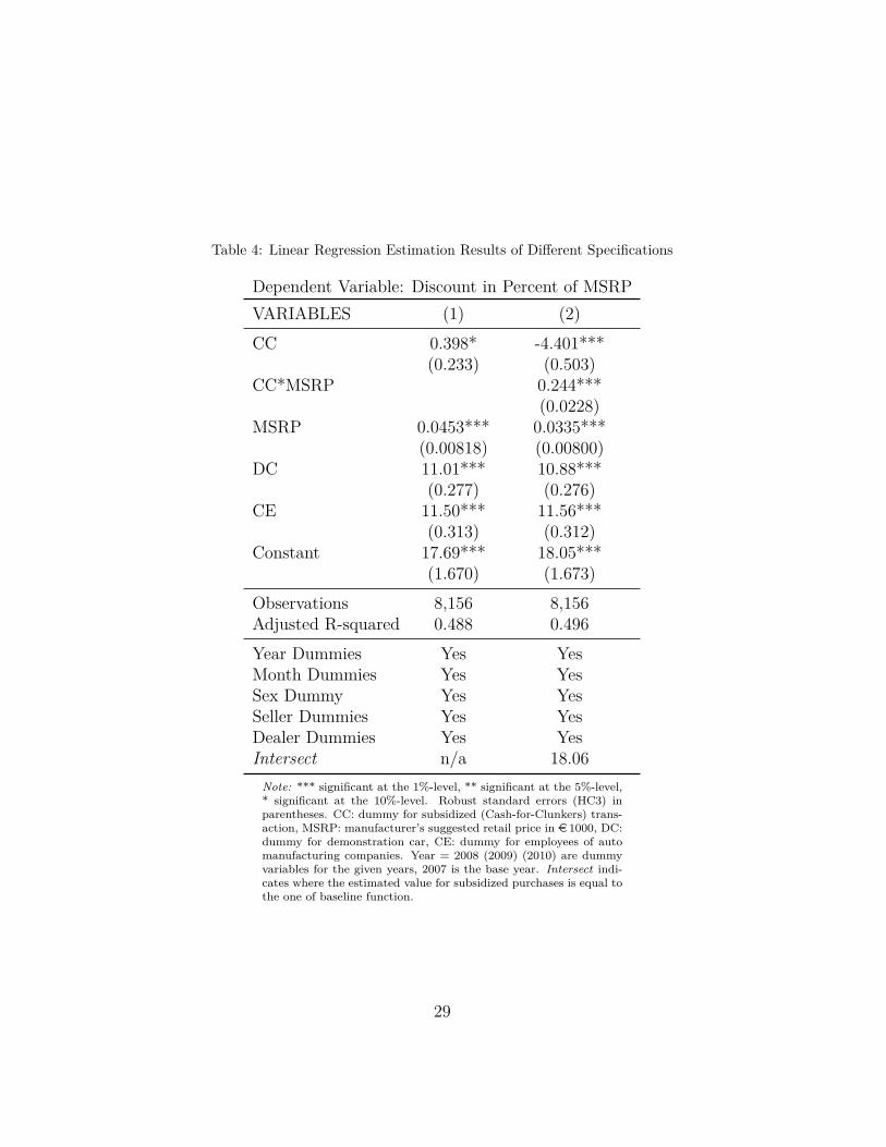
Table 4: Linear Regression Estimation Results of Different Specifications

Dependent Variable: Discount in Percent of MSRPVARIABLES (1) (2)CC 0.398* -4.401***

(0.233) (0.503)CC*MSRP 0.244***

(0.0228)MSRP 0.0453*** 0.0335***

(0.00818) (0.00800)DC 11.01*** 10.88***

(0.277) (0.276)CE 11.50*** 11.56***

(0.313) (0.312)Constant 17.69*** 18.05***

(1.670) (1.673)Observations 8,156 8,156Adjusted R-squared 0.488 0.496Year Dummies Yes YesMonth Dummies Yes YesSex Dummy Yes YesSeller Dummies Yes YesDealer Dummies Yes YesIntersect n/a 18.06

Note: *** significant at the 1%-level, ** significant at the 5%-level,* significant at the 10%-level. Robust standard errors (HC3) inparentheses. CC: dummy for subsidized (Cash-for-Clunkers) trans-action, MSRP: manufacturer’s suggested retail price in e 1000, DC:dummy for demonstration car, CE: dummy for employees of automanufacturing companies. Year = 2008 (2009) (2010) are dummyvariables for the given years, 2007 is the base year. Intersect indi-cates where the estimated value for subsidized purchases is equal tothe one of baseline function.

29

buyers (CC = 1), the function has a y-intercept of 18.05 − 4.401 = 13.65

and a slope coefficient equal to 0.2440 + 0.0335 = 0.2775. The latter line is

therefore steeper than the former but starts lower. Thus, the two functions

intersect at

Ilin = −β/δ (4)

where β measures the downward shift of the CC curve for MSRP zero,

and δ the difference between the slope of the CC and the non-CC functions.

Equation 4 therefore gives the MSRP where both functions intersect. This

value is reported at the bottom of Table 4 (Intersect), it is about e 18,000

for specification (2).

A general conclusion is that subsidized buyers of the first quartile faced

negative price discrimination, i.e., they paid more (experienced a lower dis-

count) if they received the subsidy. Since the scrappage program shifted

demand heavily to the lower-priced segments, car dealers could impose a

price markup by granting less discount. In contrast, subsidized buyers in

the third (and fourth) quartile faced positive price discrimination, meaning

they had to pay less (received more discount) if buying with the subsidy. In

this much slacker part of the car market, dealers used additional discounts

in order to seize a one-time opportunity of selling to very elastic (subsidized)

customers instead of losing them to competitors or lower car segments. At

consideration of these additional controls does not alter the results, we neglect this pointin the discussion.

30

an aggregate level, the positive price discrimination in the upper part of the

distribution overcompensates the negative effect in the lower part.36 Within

the second quartile finally, the difference between the CC and the non-CC

function is just zero. This implies that within the second quartile of MSRP,

car dealers did not price discriminate at all, and CC customers received the

full amount of the subsidy of e 2, 500.

3.5. The Relevant Price Range

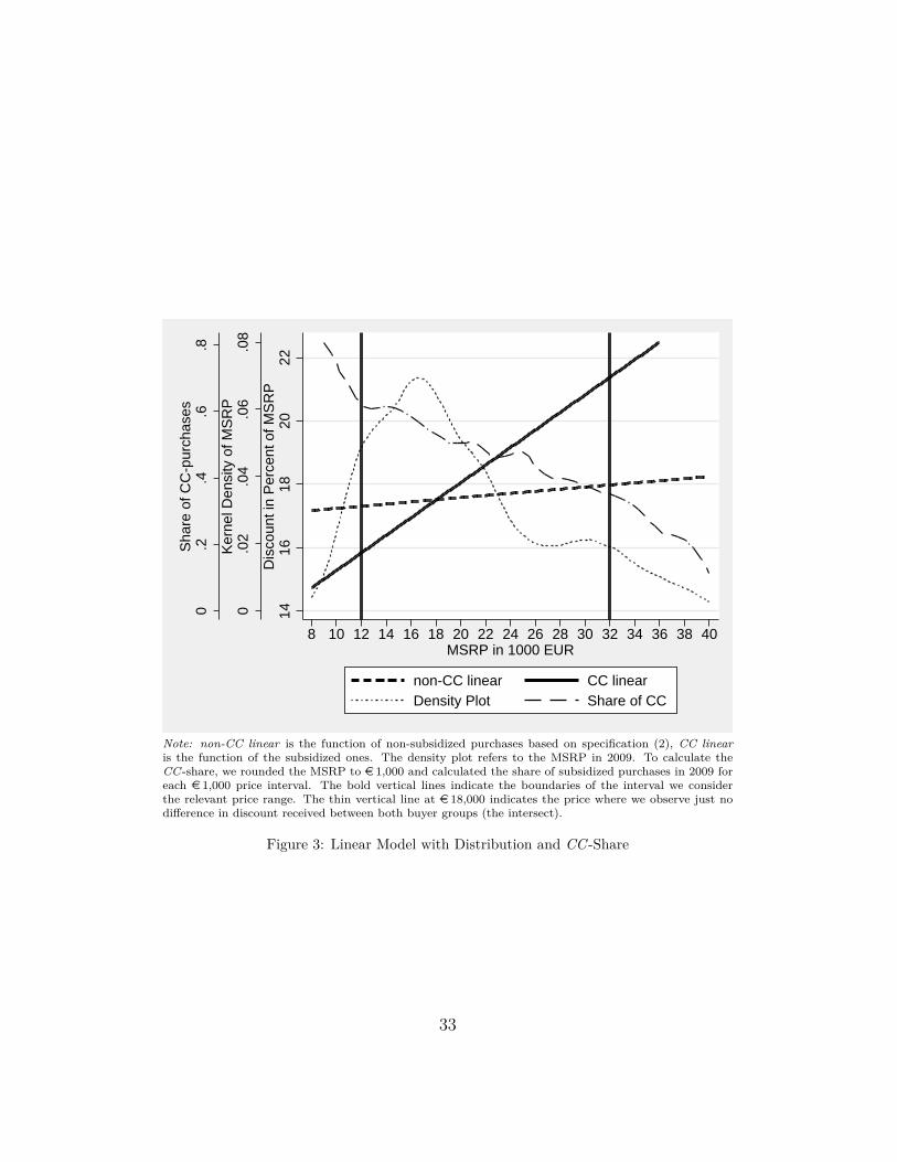
But how relevant is the region we are considering? Moreover, are subsi-

dized and non-subsidized purchases sufficiently balanced, meaning whether

the shares of CC and non-CC purchases are rather equal and therefore com-

parable? If this was not the case, our results might be misleading. Figure 3

gives an insight into the distribution and adds the share of CC purchases by

MSRP.37 The dash-dotted line shows the CC share as a falling function of

MSRP. This is what we expected, given that the lump-sum subsidy matters

relatively more for cheaper cars. However, in a region below e 12,000, the

share is larger than 60%, reaching up to 80% for cars of an MSRP of about

e 9,000. We claim that this part of the distribution lacks common support

because its composition is too unbalanced. The graph of the distribution

(dotted density plot) is very steep on the left side, which means that there

36The reported coefficient β on the CC dummy from specification (1) of Table 4 can beinterpreted as a weighted average.

37To calculate the share of CC in Figure 3, we rounded the MSRP to e 1,000 and calculatedthe share of subsidized purchases in 2009 for each e 1,000 price interval.

31

were relatively few purchases at a price range of about e 8,000, but already

quite a few at a price of e 10,000 to e 12,000. Cutting off this fringe, we see

that from an MSRP of e 12,000 on, the data points are comfortably dense

enough, and the distribution between CC and non-CC purchases is rather

balanced with about 60% or less. At the other end of the distribution, the

share of CC purchases drops below one third at a price of about e 32,000.

We choose this point as an upper bound for the following discussion. At this

point, we still observe a sufficiently balanced distribution between CC and

non-CC purchases which then steadily shrinks along with the density. In

the following discussion, we therefore focus on a price range from e 12,000

to e 32,000 which we judge to be the most relevant interval of our data with

a solid balance of CC and non-CC purchases.

3.6. Price Discrimination and Incidence

As a next step, we quantify the exact amount of price discrimination and

the corresponding incidence over the price interval for which our results were

found to be relevant. Table 5 yields an overview regarding that quantification

for the linear model (specification (2)). It provides the percentage (PD (%))

and the respective absolute (PD (e )) discount received for a certain MSRP

(what we refer to as “price discrimination”) as well as the corresponding part

(Inc (%)) of the e 2,500 subsidy which remained with the consumer (what

32

0.2

.4.6

.8S

hare

of C

C-p

urch

ases

0.0

2.0

4.0

6.0

8K

erne

l Den

sity

of M

SR

P

1416

1820

22D

isco

unt i

n P

erce

nt o

f MS

RP

8 10 12 14 16 18 20 22 24 26 28 30 32 34 36 38 40MSRP in 1000 EUR

non-CC linear CC linearDensity Plot Share of CC

Note: non-CC linear is the function of non-subsidized purchases based on specification (2), CC linearis the function of the subsidized ones. The density plot refers to the MSRP in 2009. To calculate theCC -share, we rounded the MSRP to e 1,000 and calculated the share of subsidized purchases in 2009 foreach e 1,000 price interval. The bold vertical lines indicate the boundaries of the interval we considerthe relevant price range. The thin vertical line at e 18,000 indicates the price where we observe just nodifference in discount received between both buyer groups (the intersect).

Figure 3: Linear Model with Distribution and CC -Share

33

we refer to as “incidence”).38 Recall that the point where the two groups

do not differ at all was at e 18,000. At that point the incidence is 100%, a

result that reflects the findings of Sallee (2011), for a car that would fall into

our second quartile of MSRP. For a cheap car with a MSRP of e 12,000, the

linear model yields a price discrimination of −1.48% or e−178, i.e., dealers

skimmed off about 7% of the subsidy amount (e 2,500). This translates into

an incidence amount of 93%, which would be an upper bound when compared

to the values Busse et al. (2006) find (70 − 90%).

Results for higher-priced cars are more remarkable: a car which cost

e 28,000 and therefore is at the lower end of the fourth quartile of MSRP,

would benefit from an additional discount of 2.42% or e 678, which means

that buyers received an additional discount (on top of the subsidy they re-

ceived) of around 27%. A car purchase at the very end of our relevant MSRP

range (e 32,000) caused an extra 3.4% or approximately e 1,100, which is

44% of the scrappage subsidy amount. Speaking of incidence this means

that 127% and 144% of the subsidy amount for a e 28,000 and a e 32,000

automobile “remained” with the buyer respectively. Incidence amounts lo-

cated above the 100%-threshold, in our case clearly distant from that, are

empirically rarely found.

38The Euro values were calculated from the corresponding percentage values and theMSRP, not from a separate estimation with discount in Euro as a dependent variable.

34

Table 5: Price Discrimination and Incidence over different MSRPs

MSRP PD (%) PD (e ) Inc (%)12,000 -1.48 -178 9314,000 -0.99 -139 9416,000 -0.50 -80 9718,000 -0.01 -2 10020,000 0.47 94 10424,000 1.45 348 11428,000 2.42 678 12732,000 3.40 1088 144Note: The table presents price discrimination for a given MSRP in percentage points of MSRP (PD (%))and Euro (PD (e )) based on the linear model from specification (2) as well as the respective Incidence(Inc (%)) which indicates what percentage part of the subsidy remained with the consumer.

3.7. Results

The main result of this paper is that the incidence of the subsidy strongly

and significantly varies across price segments. We focused most of our dis-

cussion on three price segments that roughly correspond to the first, second,

and third price (MSRP) quartile.39

In the first quartile that mainly covers mini cars and to some extent small

cars, subsidized buyers received slightly lower discounts than non-subsidized

ones controlling for covariates. In the second quartile—mainly consisting of

small and medium cars—discounts between the two buyer groups did not

differ much, implying that the full subsidy amount remained with the buyer.

The most striking result was found for sales in the upper half of the price

39We also consider the lower part of the fourth quartile of MSRP since we argue that ourrelevant price range reaches e 32,000.

35

distribution. We focused particularly on the third price quartile (mainly

medium and large cars), where subsidized and non-subsidized sales were quite

balanced. In this segment, scrappage premium receivers were granted much

higher discounts than regular customers. The incidence in this price segment

was such that subsidized buyers received huge extra discounts from sellers

over and above the government premium.

Our result for the lower price segments—loosely speaking for the bottom

half of the distribution—is in line with the results in Busse et al. (2006) and

Sallee (2011). Busse et al. (2006) find that between 70% and 90% of the cus-

tomer promotion amount remains with the buyer, i.e., the seller reaps only

a small fraction of the promotion. Since a customer promotion is quite com-

parable to a buyer subsidy granted by the government, the two instruments

are in fact comparable, and so are our results of roughly 90% of the subsidy

amount remaining with the buyer in the first quartile of MSRP. Sallee (2011)

finds that a customer-directed tax subsidy for the Toyota Prius, a small car

that would fall into our second price quartile, is fully captured by customers,

although sellers face a binding production constraint. In the case of the Ger-

man scrappage premium, a production constraint was also binding in the

small-car segment since the subsidy caused a run on these cars. Our results

in the second price quartile are therefore fully in line with Sallee’s results.

While his explanation builds mainly on long-run pricing policy of manufac-

turers, we conjecture that in the German case, increased competition due to

the demand shock induced by government intervention additionally explains

36

why the supply-side only captured a small or even negligible fraction of the

subsidy in the bottom half of the distribution.

In the upper price segment, non-subsidized (regular) customers did not

receive exceptional rebates since that would interfere with the well-known co-

operative pricing strategy of car manufacturers toward brand-loyal long-term

customers. This would have unnecessarily eroded margins without increas-

ing long-term demand in that customer segment. Subsidized buyers, on the

other hand, were typically not customers buying pricey cars, and would usu-

ally not upgrade from a clunker to a new expensive car. Therefore, their price

elasticity of demand for large cars was quite high, which lead the supply side

to offer exceptionally high discounts to this customer group, consistent with

our findings of incidence amounts of even more than 140%. Offering such

high rebates to subsidized customers did not interfere with long-run pricing

considerations of manufacturers since the new customer group was a one-time

target without any significant downside risk with regard to their long-run car

demand for manufacturers of large cars.

In summary, our assumptions did hold. We did see that having a clunker

is a signal that (1) you have a car at your disposal, (2) you are not likely to

target the expensive market (because you have a “clunker”) and (3) you want

to buy now, before the program expires. In the upper price segment, factor

(2) dominates and people get an extra discount because they are likely to

be price sensitive customers who differ substantially from the typical luxury

buyer. In that segment, our assumptions in terms of respective incidence

37

amounts have even been exceeded. In the cheap market, subsidized buyers

are less price elastic because they needed to buy now, whereas the non-

subsidized customer could have been more patient. Still, in that segment

dealers are not able to reap off a lot of the subsidy amount due to increased

competition in the year of the policy intervention.

4. Sensitivity Analysis

Our identification strategy employed was a simple difference design where

the discounts received by the subsidized buyers were compared to that of the

non-subsidized buyers. Hence, the assumption required for identification is

knowledge regarding what prices were actually paid by those receiving the

subsidy and a counterfactual estimate of what those people would have paid

if they had purchased the same car without the subsidy. As shown in Section

3.2, the CC and non-CC types differ significantly in almost every observable

way. The estimates in our paper control for all of these factors (company

car etc.), but it is possible that these customers also differ in unobservable

characteristics that are not controlled for and could introduce some bias.40

This is why, in the following sensitivity analysis, we challenge our results in

every reasonable way possible and present a huge variety of robustness checks

to our preferred specification.

40Certainly, the simple difference design is a limitation of that analysis. A difference-in-differences strategy would be desirable, but the CC versus non-CC group simply cannotbe established outside of the treatment period, i.e., for years other than 2009.

38

So far, the presented results restrict the econometric model to a linear

form which might be too inflexible. We therefore present a quadratic version

of the same underlying economic model as well as a reformulation to a log-

linear model. Beyond the functional form, the results might be driven by

(neglected) time effects or by subgroups, or they might be sensitive to the

transformation of the data. Below, we show that a more flexible estimation

would not yield economically different results. A log-lin version of the same

model would actually yield a bigger effect, i.e., a stronger negative price

discrimination for cheaper cars and a stronger positive discrimination for

purchases of expensive cars. We also present sensitivity checks including

additional time controls, interactions, or restricting the data to 2009 and

the relevant price range. After that, we successively drop subsets of the

data which could be driving the results and show results for a variety of

quantile regressions. The results are qualitatively insensitive to any of these

robustness checks.

In a first step, we run a quadratic specification of the model as given in

Equation (5).

discount = α + βCC + γ1MSRP + γ2MSRP 2+

δ1CC ∗MSRP + δ2(CC ∗MSRP )2 + θ′X + ε

(5)

Rather than comparing the coefficients of the model, we present the plot

of the linear and the quadratic model in Figure 4 based on the estimated

39

1520

2530

Dis

coun

t in

Per

cent

of M

SR

P

10 20 30 40 50 60MSRP in 1000 EUR

non-CC linear CC linearnon-CC quadratic CC quadratic

Note: Expected discount in percent as a function of MSRP. Functions are given over two models (linearand quadratic) and two groups, subsidized (CC) and non-subsidized (non-CC) transactions. Parametersare taken from the regression results above, specifications (2) (linear) and (3) (quadratic). The dashedvertical lines show the upper borders of the first, the second, and the third quartiles of MSRP in 2009.The solid vertical lines show the intersects between the CC and non-CC functions, i.e., the prices wherewe observe just no difference in discount received between both buyer groups.

Figure 4: Linear and Quadratic Model for Year 2009

40

coefficients.41 We first plot the reference line, i.e., the discount in percent as

a function of MSRP for the two models. These are the lower dashed functions

in the graph, and one can see that they hardly differ. The upper functions

are the respective subsidized purchases where there is a little more difference

between the two models. The dashed vertical lines show the borders of the

first, the second, and the third quartile of MSRP in 2009. The two functions

diverge only from a price of roughly e 40,000 on, and are very close to each

other even for rather low prices of about e 10,000. The divergence in the

upper part is of little importance as the scrappage premium did not play

an important role in these price ranges.42 The vertical solid lines show the

intersects between the CC and non-CC functions, i.e., the point where there

is no difference in discount between a purchase with and without the subsidy.

One can see that in both cases the intersect is located within the second

quartile at a price of about e 18,000 and both functions differ little within

what we defined as the relevant price range in Section 3.5.

As the functional form appears adequate for the observed data, we run a

battery of tests on the linear model as given in Equation (3). Table 6 sums

up the tests we ran on our data sample. It reports the most relevant fig-

41Regression results for the quadratic or even cubic formulation of the model are availableupon request.

42There are two major reasons for this: first, the relative importance of the lump-sumsubsidy decreases as the car price increases. Second, as the subsidy could only berequested when an old car was scrapped, the old car needed to be of a very low resalevalue. In general, buyers of expensive cars benefited more from trading in their old carthan scrapping it for e 2,500.

41

ures: the number of observations (Obs.), the intersect, i.e., the point where

there is no difference in discount between a subsidized and a non-subsidized

car (Inters.), the coefficient for the scrappage premium (CC ), the coefficient

of the interaction term (CC*MSRP), and the percentage levels of price dis-

crimination for a e 12,000, an e 18,000, and a e 32,000 car purchase (PD12,

PD18 and PD32 ).43

The first row represents the linear model based on the full data, i.e., the

reference results from Specification (2) in Table 4. In the second row, we

present an alternative specification of the model. Instead of regressing the

discount in percent, we regress the logarithm of the discount in Euro on the

model as discussed above.44 This specification is more flexible and less liable

to extreme values. However, as we observe the discount to be zero in some

two hundred cases, we lose these observations. We can see that the intersect

changes little (it is actually rather big at 19.63). The coefficients of CC

and the interaction term cannot be compared to the others due to the log-

transformation, but they do show the expected sign and order of magnitude.

The observed price discrimination is even more pronounced than in the linear

model. We find −3.65% for an MSRP of e 12,000, −.69% for e 18,000 and

5.72% for e 32,000. This indicates that our preferred estimated results are a

lower bound, and hence a rather conservative measure, of the actual effect.

43Full regression tables are available upon request.44For some variables which imply a level-effect in the discount in percent, such as thecontrol for demonstration cars or company employees, we add an interaction betweenthe MSRP and the respective dummy.

42

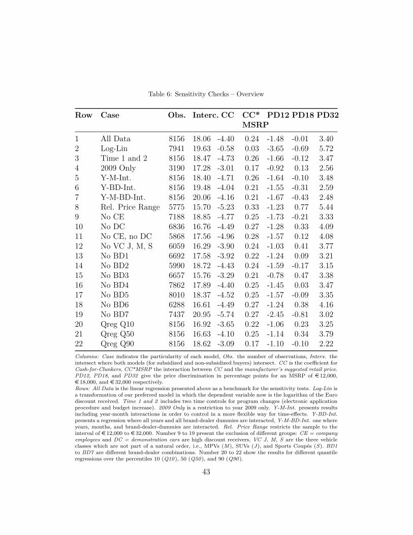
Table 6: Sensitivity Checks – Overview

Row Case Obs. Interc. CC CC* PD12 PD18 PD32MSRP

1 All Data 8156 18.06 -4.40 0.24 -1.48 -0.01 3.402 Log-Lin 7941 19.63 -0.58 0.03 -3.65 -0.69 5.723 Time 1 and 2 8156 18.47 -4.73 0.26 -1.66 -0.12 3.474 2009 Only 3190 17.28 -3.01 0.17 -0.92 0.13 2.565 Y-M-Int. 8156 18.40 -4.71 0.26 -1.64 -0.10 3.486 Y-BD-Int. 8156 19.48 -4.04 0.21 -1.55 -0.31 2.597 Y-M-BD-Int. 8156 20.06 -4.16 0.21 -1.67 -0.43 2.488 Rel. Price Range 5775 15.70 -5.23 0.33 -1.23 0.77 5.449 No CE 7188 18.85 -4.77 0.25 -1.73 -0.21 3.3310 No DC 6836 16.76 -4.49 0.27 -1.28 0.33 4.0911 No CE, no DC 5868 17.56 -4.96 0.28 -1.57 0.12 4.0812 No VC J, M, S 6059 16.29 -3.90 0.24 -1.03 0.41 3.7713 No BD1 6692 17.58 -3.92 0.22 -1.24 0.09 3.2114 No BD2 5990 18.72 -4.43 0.24 -1.59 -0.17 3.1515 No BD3 6657 15.76 -3.29 0.21 -0.78 0.47 3.3816 No BD4 7862 17.89 -4.40 0.25 -1.45 0.03 3.4717 No BD5 8010 18.37 -4.52 0.25 -1.57 -0.09 3.3518 No BD6 6288 16.61 -4.49 0.27 -1.24 0.38 4.1619 No BD7 7437 20.95 -5.74 0.27 -2.45 -0.81 3.0220 Qreg Q10 8156 16.92 -3.65 0.22 -1.06 0.23 3.2521 Qreg Q50 8156 16.63 -4.10 0.25 -1.14 0.34 3.7922 Qreg Q90 8156 18.62 -3.09 0.17 -1.10 -0.10 2.22Columns: Case indicates the particularity of each model, Obs. the number of observations, Inters. theintersect where both models (for subsidized and non-subsidized buyers) intersect. CC is the coefficient forCash-for-Clunkers, CC*MSRP the interaction between CC and the manufacturer’s suggested retail price.PD12, PD18, and PD32 give the price discrimination in percentage points for an MSRP of e 12,000,e 18,000, and e 32,000 respectively.Rows: All Data is the linear regression presented above as a benchmark for the sensitivity tests. Log-Lin isa transformation of our preferred model in which the dependent variable now is the logarithm of the Eurodiscount received. Time 1 and 2 includes two time controls for program changes (electronic applicationprocedure and budget increase). 2009 Only is a restriction to year 2009 only. Y-M-Int. presents resultsincluding year-month interactions in order to control in a more flexible way for time-effects. Y-BD-Int.presents a regression where all years and all brand-dealer dummies are interacted, Y-M-BD-Int. one whereyears, months, and brand-dealer-dummies are interacted. Rel. Price Range restricts the sample to theinterval of e 12,000 to e 32,000. Number 9 to 19 present the exclusion of different groups: CE = companyemployees and DC = demonstration cars are high discount receivers, VC J, M, S are the three vehicleclasses which are not part of a natural order, i.e., MPVs (M), SUVs (J), and Sports Coupés (S). BD1to BD7 are different brand-dealer combinations. Number 20 to 22 show the results for different quantileregressions over the percentiles 10 (Q10 ), 50 (Q50 ), and 90 (Q90 ).

43

For the ease of interpretation, we stick to the preferred model where we model

the dependent variable as the discount in percentage of the MSRP.

In row three, we add two time controls to the model: a dummy for the

switch from the paper-based to the electronic subsidy application procedure

(Time 1 ) and a time dummy for the expansion of the program from e 1.5

to e 5 Billion (Time 2 ). One can see that the inclusion of these further

controls does not alter the results significantly. In row four, we restrict our

sample to year 2009 only. While the price discrimination measured for an

MSRP of e 12,000 is slightly lower, the overall pattern remains the same.

This indicates that we do not simply observe a difference because 2009 was

very special, but that the hypothesis of price discrimination actually holds.

Rows five to seven present more flexible versions of the model. In row five,

we allow for different seasonal effects by interacting year and time dummies.

In row six, we interact brand-dealership combinations with year dummies in

order to allow for differences between the dealerships and over time. In row

seven, we interact all three sets of dummies, i.e., years, months, and brand-

dealership combinations. This means we allow for different time effects over

the brand-dealership combinations and we allow these effects to be different

over the years. The coefficients and hence the measured price discrimination

do not change significantly.

As discussed in Section 3.5, the price range for which our results are

most reliable is the interval between e 12,000 and e 32,000 (MSRP). In row

eight, we therefore restrict the sample to this price range in order to make

44

sure our results are not driven by values far away from what we called the

relevant price range. The restriction makes the CC -function steeper, but

the intersect even smaller. So even though the intersect shifts leftward to

15.7, the observed price discrimination shows the same pattern and same

magnitude as our reference estimates in row one.

As already discussed, our results might be affected by composition ef-

fects stemming from unequal shares of high-discount groups. In addition to

correcting for different levels of discount (note that the coefficients are very

stable over all considered specifications), we exclude both groups from the

regression: first, company employees (No CE, row nine), then demonstration

cars (No DC, row ten) and, in row eleven, both. None of these exclusions

changes the results significantly.

In row twelve, we exclude the three vehicle classes that do not enter the

“natural” order. These are SUVs (J ), MPVs (M ) and Sports Coupés (S).45

Again, the results stay unaffected.

Rows 13-19 show the results when leaving out single brand-dealer com-

binations. They illustrate that the results of our analysis are not driven by

a single group of those categories. The intersect is rather stable over the

different data restrictions: it may fall down to about e 16,000 (row 15), but

can also move up to roughly e 21,000 (row 19). On average however, it is

45The other vehicle classes are cardinally ordered by size and, most important, price. Thethree excluded vehicle classes are not part of this order and might be special for variousreasons.

45

located around e 17,000 to e 18,000, and therefore meets the dimension of

our full model.

Even though the dependent variable (discount in percent of MSRP) is

almost normally distributed, it is not perfectly so, and it is possible that

the observed effect is not only heterogeneous over MSRP, but also over the

dependent variable. Rows 20-22 therefore present the results from quantile

regressions over the 10th, 50th, and 90th percentile. We can see that the

results do not change either.46

Overall, Table 6 demonstrates that our findings are robust to an exten-

sive variety of sensitivity checks. The log-linear specification shows that

our preferred estimates are rather conservative. Also, it is unlikely that

the presented estimation results are caused by the functional form, ignored

program influences, differences over time, high discount groups or special

vehicle classes, nor single dealers or brands. Quantile regressions confirm

the reported results. In addition to robust standard errors, we also ran

our preferred regression with standard errors clustered either by brand, by

brand-dealer combination, or by year.47 All relevant coefficients remain sig-

nificant.48

46Table 6 does not report significance levels, but all relevant coefficients, i.e., the coeffi-cients for CC, MSRP and the interaction are significant at the 1% level.

47We do this since treating each car sold as a completely independent observation couldtend to be too permissive.

48In all cases, the coefficient for CC is still significant at the 5%-level and the interactionterm remains significant at the 1%-level. Only the coefficient for MSRP, which is notcrucial for our results, turns insignificant. .

46

We conclude from the robustness analysis that our results are not driven

by unobserved heterogeneity or misspecification. Overall, the preferred model

appears to be rather conservative. The model controls for most relevant in-

fluences, with the price of the car being the most important feature.

5. Conclusion

We evaluate the incidence of the German scrappage program from 2009,

the most expensive program of all countries in that time period with a to-

tal volume of e 5 billion ($7 billion). Overall, we find that the benefits—as

intended—are captured by the customers, with this effect being heteroge-

neous over price segments.

Applying linear regression models to a unique sample of micro transac-

tion data, we model the percentage discount as a function of the MSRP, a

dummy for the scrapping premium, and various controls. In a first step, we

find that, on average, the subsidy is captured by the customers by slightly

more than 100%. We therefore allow for heterogeneity across price segments

when comparing subsidized to non-subsidized purchases and find that these

differ significantly. Subsidized buyers of the first quartile (cheap cars) faced

negative price discrimination, i.e., received less discount than non-subsidized

buyers, leaving them with incidence amounts smaller than 100%. Above the

median MSRP (up to expensive cars), the discount for subsidized buyers was

higher than the discount for non-subsidized ones, i.e., Cash-for-Clunkers cus-

tomers faced positive price discrimination or incidence amounts of more than

47

100%. The absolute amount of price discrimination was substantially bigger

in the upper range of MSRP. Our results can be explained by an optimal

pricing strategy of the supply side which depends on market segments and

different price elasticities of demand.

With regard to the incidence, we showed that the supply-side captured a

small fraction of the subsidy, but only for cars from smaller vehicle classes.

For bigger, more expensive cars, the customers received additional discounts

in order to sign a contract of purchase. In summary, the car industry bene-

fited by selling additional cars, and consumers benefited by being subsidized

by the government and the industry. However, not all consumers benefited

by the same amount and, as the program was tax-financed, most of those

who bore the costs did not benefit from it at all.

While our findings are very robust to changes in the model as well as

different data restrictions, they can only shed light on what happened in

the market of new cars. The demand shock for new cars obviously had

repercussions on the used car market and, as the maintenance of new cars is

usually done by manufacturer-related subcontractors, we also expect negative

impacts on repair shops which are not linked to a particular manufacturer.

Since we do not have data and sufficient information in these respects, we

cannot go into a thorough welfare analysis and therefore strictly separate

efficiency questions from our incidence focus.

48

Appendix

49

Table A1: Number of Purchases over Car Brands and Car Dealers

Car BrandCar Dealer 1 2 3 4 5 6 TotalDealer 1 0 2166 0 0 0 0 2166Dealer 2 1464 0 0 0 0 0 1464Dealer 3 0 1499 0 0 0 0 1499Dealer 4 0 0 0 0 1868 0 1868Dealer 5 0 0 294 0 0 0 294Dealer 6 0 0 0 146 0 719 865Total 1464 3665 294 146 1868 719 8156

50

Table A2: Number of Purchases over Month of all Years, 2009 by CC

Year of Purchase and Clunker’s Premium2007 2008 2009 2009 2010

Month of Purchase Non-CC

CC

1 103 109 115 25 1012 85 132 139 93 1203 162 175 183 206 2304 154 225 157 200 1595 147 159 115 221 1836 142 172 156 198 1667 118 149 129 192 1338 116 85 107 150 1339 140 115 136 102 12910 109 145 145 100 14311 134 120 137 41 11412 144 115 130 13 100Total 1554 1701 1649 1541 1711Note: Non-CC are non-subsidized purchases, CC subsidized ones.

51

Table A3: Summary Statistics over Vehicle Class

Catalog price in 1.000 EUREU Vehicle Class Mean SD NA - Mini Cars 11.59 1.29 649B - Small Cars 16.09 2.59 2611C - Medium Cars 23.76 4.22 1649D - Large Cars 38.94 7.87 899E - Executive Cars 58.32 11.54 232F - Luxury Cars 106.91 15.54 19J - SUV 40.18 14.68 481M - MPV 27.25 7.28 1429S - Sports Coupés 61.09 25.51 187Total 25.62 14.37 8156Note: SUV stands for Sport Utility Vehicle, MPV for Multi Purpose Vehicle.

52

Table A4: Summary Statistics: 2009 Only

Variables Mean SD Med Min Max NDiscount in Percent 17.11 7.82 16.75 0.00 45.61 3,190Discount in 1000 EUR 3.99 3.20 3.25 0.00 51.81 3,190MSRP in 1000 EUR 23.02 12.76 19.25 8.69 130.35 3,190Clunker’s Premium (CC) 0.48 0.50 0 0 1 3,190Demonstration Car (DC) 0.14 0.35 0 0 1 3,190Company Employee (CE) 0.13 0.33 0 0 1 3,190Female 0.32 0.46 0 0 1 3,190Age at Purchase 46.79 15.09 48 18 89 639Note: MSRP is the manufacturer suggested retail price. CC is a dummy variable indicating whether thebuyer of a car received the scrappage subsidy. DC is a dummy variable indicating whether a buyer boughta demonstration car. CE is a dummy variable indicating whether the buyer was an employee of a carmanufacturing company. Female is a dummy of female buyers, the summary statistics therefore reportthe share of women, age at purchase is the age of the buyer at the time of purchase.

53

Table A5: Percentage Discount over Time by CC

Discount in PercentNon-CC CC Total

Year of Purchase MeanSD N MeanSD N MeanSD N2007 15.69 9.01 1554 0 15.69 9.01 15542008 16.54 9.64 1701 0 16.54 9.64 17012009 17.67 8.73 1649 16.51 6.67 1541 17.11 7.82 31902010 18.03 8.74 1711 0 18.03 8.74 1711Total 17.01 9.09 6615 16.51 6.67 1541 16.91 8.68 8156Note: Non-CC are non-subsidized purchases, CC subsidized ones. The last three columns of the tablegive summary statistics for the whole group.

54

Table A6: Percentage Discount by Type of Purchase

Discount in PercentType of Purchase Mean SD NStandard 14.02 7.44 5868Company Employee 25.84 4.03 968Demonstration Car 23.25 8.47 1320Total 16.91 8.68 8156Note: Standard are the benchmark purchases, Company Employees are employees of a car manufacturingcompany, Demonstration Car denotes cars that are not new but have been used for exhibition and havebeen licensed for a maximum of 14 months before the purchase.

55

050

0000

1000

000

A -

Min

i Car

s

B -

Sm

all C

ars

C -

Med

ium

Car

s

D -

Lar

ge C

ars

E -

Exe

cutiv

e C

ars

F -

Lux

ury

Car

s

J -

SU

V

M -

MP

V

S -

Spo

rts

Cou

pés

2008 2009 2010

Num

ber

of N

ew R

egis

trat

ions

Year of Registration

Note: A, B, C, D, E, F, J, M, S are auto segments according to the EU car classification. SUV standsfor Sport Utility Vehicle, MPV for Multi Purpose Vehicle.

Figure A1: All New Car Registrations in Germany over Time by Vehicle Class

56

10.511

11.512

12.5

15

16

17

18

2223242526

30

35

40

45

50

60

70

80

100

110

120

130

30

40

50

60

20

25

30

5060708090

2007q1 2008q1 2009q1 2010q1 2011q1 2007q1 2008q1 2009q1 2010q1 2011q1 2007q1 2008q1 2009q1 2010q1 2011q1

A - Mini Cars B - Small Cars C - Medium Cars

D - Large Cars E - Executive Cars F - Luxury Cars

J - SUV M - MPV S - Sports Coupés

Non-CC transactions CC transactions

MS

RP

in 1

000

EU

R

Quarter of Purchase

Note: MSRP over quarters of years across EU vehicle classes. SUV stands for Sport Utility Vehicle, MPVfor Multi Purpose Vehicle. The graphs show mean values rounded by quarter.

Figure A2: MSRP over Time by EU Vehicle Class

57

References

Adda, J. and R. Cooper, “Balladurette and Juppette: A Discrete Analysis

of Scrapping Subsidies,” Journal of Political Economy, August 2000, 108

(4), 778–806.

Anderson, Simon P., Andre de Palma, and Brent Kreider, “Tax Inci-

dence in Differentiated Product Oligopoly.,” Journal of Public Economics,

2001, 81 (2), 173 – 192.

Berry, Steven, James Levinsohn, and Ariel Pakes, “Automobile Prices

in Market Equilibrium,” Econometrica, 1995, 63 (4), 841–890.

Böckers, Veit, Ulrich Heimeshoff, and Andrea Müller, “Pull-forward

effects in the German car scrappage scheme: A time series approach,”

DICE Discussion Papers 56, Heinrich-Heine-Universität Düsseldorf, Düs-

seldorf Institute for Competition Economics (DICE) 2012.

Busse, Meghan, Jorge Silva-Risso, and Florian Zettelmeyer, “$1,000

Cash Back: The Pass-Through of Auto Manufacture Promotions,” The

American Economic Review, September 2006, 96 (4), 1253–1253.

Busse, Meghan R., Christopher R. Knittel, Jorge Silva-Risso, and

Florian Zettelmeyer, “Did ’Cash for Clunkers’ Deliver? The Consumer

Effects of the Car Allowance Rebate System,” November 2012. Working

Paper.

58

Chetty, Raj, Adam Looney, and Kory Kroft, “Salience and Taxation:

Theory and Evidence,” The American Economic Review, 2009, 99 (4),

1145–1177.

Delipalla, Sophia and Owen O’Donnell, “Estimating Tax Incidence,

Market Power and Market Conduct: The European Cigarette Industry.,”

International Journal of Industrial Organization, 2001, 19 (6), 885 – 908.

Deysher, Beth and Don Pickrell, “Emissions Reductions From Vehicle

Retirement Programs,” Transportation Research Record: Journal of the

Transportation Research Board, 1997, 1587, 121–127.

Evans, William N., Jeanne S. Ringel, and Diana Stech, “Tobacco

Taxes and Public Policy to Discourage Smoking,” in “Tax Policy and the

Economy,” Vol. 13 of NBER Chapters, National Bureau of Economic Re-

search, Inc, 1999, pp. 1–56.

Friedman, John, “The Incidence of the Medicare Prescription Drug Benefit:

Using Asset Prices to Assess its Impact on Drug Makers,” 2009. Working

Paper, Harvard Kennedy School, Harvard University.

Fullerton, Don and Gilbert E. Metcalf, “Tax Incidence,” in Alan J.

Auerbach and Martin Feldstein, eds., Handbook of Public Economics, Vol. 4

of Handbook of Public Economics, Elsevier, 2002, pp. 1787–1872.

59

Goldberg, Pinelopi Koujianou, “Product Differentiation and Oligopoly

in International Markets: The Case of the U.S. Automobile Industry,”

Econometrica, July 1995, 63 (4), 891–951.

Goldberg, Pinelopi Koujianou, “Dealer Price Discrimination in New Car

Purchases: Evidence from the Consumer Expenditure Survey,” Journal of

Political Economy, June 1996, 104 (3), 622–654.

Hahn, Robert W., “An Economic Analysis of Scrappage,” The RAND

Journal of Economics, 1995, 26 (2), 222–242.

Hastings, Justine and Ebonya Washington, “The First of the Month

Effect: Consumer Behavior and Store Responses,” American Economic

Journal: Economic Policy, May 2010, 2 (2), 142–162.

Heimeshoff, Ulrich and Andrea Müller, “Evaluating the Causal Effects

of Cash-for-Clunkers Programs in Selected Countries: Success or Failure?,”

2011. Working Paper.

Kavalec, Chris and Winardi Setiawan, “An analysis of accelerated ve-

hicle retirement programs using a discrete choice personal vehicle model,”

Transport Policy, 1997, 4 (2), 95–107.

Knittel, Christopher R., “The Implied Cost of Carbon Dioxide Under

the Cash for Clunkers Program,” 2009. Working Paper, Sloan School of

Management, Massachusetts Institute of Technology.

60

Kotlikoff, Laurence J. and Lawrence H. Summers, “Tax Incidence,”

in Alan J. Auerbach and Martin Feldstein, eds., Handbook of Public Eco-

nomics, Vol. 2 of Handbook of Public Economics, Elsevier, 1987, pp. 1043–

1092.

Li, Shanjun, Joshua Linn, and Elisheba Spiller, “Evaluating ’Cash-for-

Clunkers’: Program Effects on Auto Sales and the Environment.,” Journal

of Environmental Economics and Management, 2013, 65 (2), 175 – 193.

Licandro, Omar and Antonio R. Sampayo, “The Effects of Replacement

Schemes on Car Sales: The Spanish Case,” Investigaciones Economicas,

May 2006, 30 (2), 239–282.

Marion, Justin and Erich Muehlegger, “Fuel tax incidence and supply

conditions,” Journal of Public Economics, 2011, 95, 1202–1212.

Mian, Atif and Amir Sufi, “The Effects of Fiscal Stimulus: Evidence from

the 2009 Cash for Clunkers Program.,” Quarterly Journal of Economics,

2012, 127 (3), 1107 – 1142.

Rothstein, Jesse, “Is the EITC as Good as an NIT? Conditional Cash

Transfers and Tax Incidence,” American Economic Journal: Economic

Policy, 2010, 2 (1), 177–208.

Ruffle, Bradley J., “Tax and subsidy incidence equivalence theories: exper-

imental evidence from competitive markets,” Journal of Public Economics,

2005, 89, 1519–1542.

61

Sallee, James M., “The Surprising Incidence of Tax Credits for the Toyota

Prius,” American Economic Journal: Economic Policy, May 2011, 3 (2),

189–219.

Stern, Nicholas H., “The Effects of Taxation, Price Control and Govern-

ment Contracts in Oligopoly and Monopolistic Competition.,” Journal of

Public Economics, 1987, 32 (2), 133 – 158.

Sudhir, K., “Competitive Pricing Behavior in the Auto Market: A Struc-

tural Analysis,” Marketing Science, 2001, 20 (1), 42–60.

Szwarcfiter, Lila, Francisco Eduardo Mendes, and Emilio Lebre La

Rovere, “Enhancing the Effects of the Brazilian Program to Reduce At-

mospheric Pollutant Emissions from Vehicles,” Transportation Research:

Part D: Transport and Environment, 2005, 10 (2), 153–160.

Verboven, Frank, “Quality-Based Price Discrimination and Tax Incidence:

Evidence from Gasoline and Diesel Cars,” The RAND Journal of Eco-

nomics, 2002, 33 (2), 275–297.

62