ELSEVIF_~

An International Joumal Available online at www.sciencedirectcom computers &

.¢,..=.~---(-~o,.=cT. mathematics with applicaUons

Computers and Mathematics with Applications 48 (2004) 1643-1649 www.elsevier.com/locate/camwa

The Incidence Coloring N umbers of Meshes*

CHENG-I. HUANG Department of Electronic Engineering

National Taiwan University of Science and Technology Taipei, Taiwan, R.O.C.

YuE-LI WANG t Department of Information Management

National Taiwan University of Science and Technology 43, Section 4, Kee-Lung Road, Taipei, Taiwan, R.O.C.

ecdir~mail, ntust, edu. tw

SHENG-SHIUNG CHUNG Department of Information Management

National Taiwan University of Science and Technology Taipei, Taiwan, R.O.C.

(Received September 2003; revised and accepted February 2004)

A b s t r a c t - - B r u a l d i and Massey defined the incidence coloring number of a graph and bounded it by the maximum degree. They conjectured that every graph can be incidence colored with A + 2 colors, where A is the maximum degree of a graph. Guiduli disproved the conjecture. However, Shiu et el. considered graphs with A = 3 and showed that the conjecture holds for cubic Hamiltonian graphs and some other cubic graphs. This work presents methods of incidence coloring of square meshes, hexagonal meshes, and honeycomb meshes. The meshes can be incidence colored with A + 1 colors. (~) 2004 Elsevier Ltd. All rights reserved.

K e y w o r d s - - I n t e r c o n n e c t i o n networks, Honeycomb meshes, Hexagonal meshes, Square meshes, Incidence coloring.

1. I N T R O D U C T I O N

This investigation addresses the incidence coloring numbers of several classes of meshes--namely square meshes, hexagonal meshes, and honeycomb meshes. Brualdi and Massey defined the inc idence color ing n u m b e r [1]. T h e set of incidences for a g r aph G = (V, E ) is t h e set I a --

{(v, e) : v E V, e 6 E , v is inc ident w i th e}, where V and E are t he v e r t e x and edge, respect ively,

sets of G. T w o incidences (vl , e l ) and (v2, e2) are adjacent if one of t he fol lowing holds:

(1) v l = v2,

(2) e l = e 2 , and

(3) t he edge vlv2 equals to e l or e2.

*This research was partially supported by National Science Council under the Grant NSC91-2213-E-011-044. tAuthor to whom all correspondence should be addressed.

0898-1221/04/$ - see front matter (~) 2004 Elsevier Ltd. All rights reserved. Typeset by .AM, S-TEX d oi: 10.1016/j. camwa. 2004.02.006

1644 C.-I. HUANG et al.

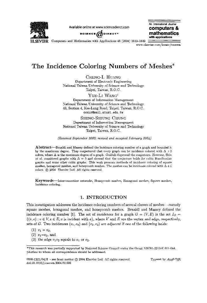
An incidence coloring function ~ of G is a mapping from i c to a color set C, such that ad- jacent incidences of G are assigned distinct colors. For example, a(v, e) = Cl means that the incidence (v, e) is colored with color Cl. The incidence coloring number of G, denoted by xi(G), is the smallest number of colors in incidence coloring. See Figure 1 for an illustration. The graph G in Figure 1 has six vertices Vl,V2,.. . ,v6 and seven edges e l ,e2 , . . . , eT. The inci- dence set I c = {(Vl, el), (v~, e3), (v2, el), (V2, e2) , (v2, e4), • • • }. The adjacent incidences of (v2, e2)

are (v2, el), (v2, e4) , (v3, e2) , and (va, es). The incidence colors are ~(vl, el) = c4, a(vl, e3) =

ca, a(v2, el) = ca, and so on. Since four colors are the smallest incidence coloring number for G,

x~( G) = 4.

Vl c4 cl v2 c3 c4 v3

e3 e4 e5

c e 6 4 e7 c3

~4 c2 c3 v5 Cl c2 v6

Figure 1. A graph with incidence coloring.

Brualdi and Massey conjectured that xi(G) <_ A+2 for every graph G, where A is the maximum degree of a graph [1]. In [2], Guiduli showed that the concept of incidence coloring is a special case of directed star arboricity, as introduced by Algor and Alon [3], and gave a counterexample to show that x~(G) _< A + O(lg A). In [4], Shiu et al. considered graphs with A = 3 and showed that the conjecture in [1] holds for cubic Hamiltonian graphs and some other cubic graphs.

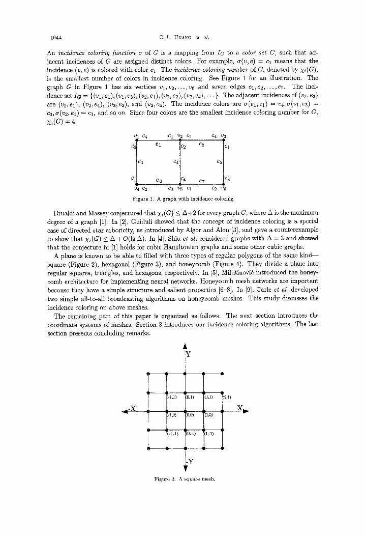
A plane is known to be able to filled with three types of regular polygons of the same kind-- square (Figure 2), hexagonal (Figure 3), and honeycomb (Figure 4). They divide a plane into regular squares, triangles, and hexagons, respectively. In [5], Milutinovid introduced the honey- comb architecture for implementing neural networks. Honeycomb mesh networks are important because they have a simple structure and salient properties [6-8]. In [9], Carle et al. developed two simple all-to-all broadcasting algorithms on honeycomb meshes. This study discusses the incidence coloring on above meshes.

The remaining part of this paper is organized as follows. The next section introduces the coordinate systems of meshes. Section 3 introduces our incidence coloring algorithms. The last section presents concluding remarks.

:-1,1)

:- 19)

(-1,-1)

I 0,1) (1,1)

0,0) (1,0)

I0;1) • :1,-1)

-y

i2,1)

Figure 2. A square mesh.

The Incidence Coloring Numbers 1645

Z ~- -Z

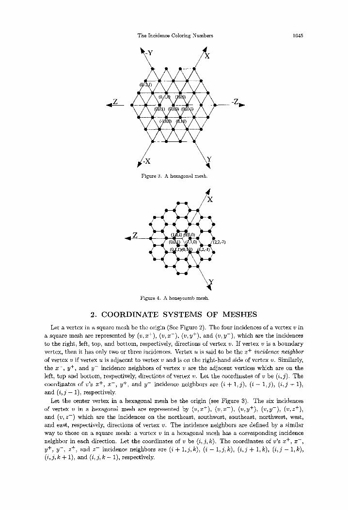
Figure 3. A hexagonal mesh.

_..Z

X

2 2) 7--

Figure 4. A honeycomb mesh.

2. C O O R D I N A T E S Y S T E M S OF M E S H E S

Let a vertex in a square mesh be the origin (See Figure 2). The four incidences of a vertex v in a square mesh are represented by (v, x+), (v, x - ) , (v, y+), and (v, y-) , which are the incidences to the right, left, top, and bot tom, respectively, directions of vertex v. If vertex v is a boundary vertex, then it has only two or three incidences. Vertex u is said to be the x + incidence neighbor of vertex v if vertex u is adjacent to vertex v and is on the right-hand side of vertex v. Similarly, the x - , y+, and y - incidence neighbors of vertex v are the adjacent vertices which are on the left, top and bot tom, respectively, directions of vertex v. Let the coordinates of v be (i,j). The coordinates of v's x +, x - , y+, and y - incidence neighbors are (i + 1, j ) , (i - 1 , j ) , (i,j + 1), and ( i , j - 1), respectively.

Let the center vertex in a hexagonal mesh be the origin (see Figure 3). The six incidences of vertex v in a hexagonal mesh are represented by (v,x+), (v ,x- ) , (v,y+), (v ,y-) , (v,z+), and (v, z - ) which are the incidences on the northeast, southwest, southeast, northwest, west, and east, respectively, directions of vertex v. The incidence neighbors are defined by a similar way to those on a square mesh: a vertex v in a hexagonal mesh has a corresponding incidence neighbor in each direction. Let the coordinates of v be (i, j , k). The coordinates of v's x +, x - , y+, y- , z +, and z - incidence neighbors are (i ÷ 1, j, k), (i - 1, j, k), (i, j ~- 1, k), ( i , j - 1, k), (i,j, k ÷ 1), and (i,j, k - 1), respectively.

1646 C.-I. HUANG et al.

For a honeycomb mesh, we use the coordinate system introduced by Stojmenovic [8]. Let x-, y-, and z-axes start at the center of the honeycomb mesh and be parallel to the three edge directions, respectively (see Figure 4). The size t of a honeycomb mesh is the number of layers from its center to its boundary. For example, t = 3 for the honeycomb mesh in Figure 4. The vertices of a honeycomb mesh can be coded using integer triples (i, j, k), such that - t + 1 _< i, j, k _< t and 1 < i + j + k _< 2. If i + j + k = 1, then the coordinates of v's x +, y+, and z + incidence neighbors are (i + 1,j, k), (i,j + 1, k), and (i,j, k + 1), respectively. If i + j + k = 2, then the coordinates of v's x , y , and z- incidence neighbors are (i - 1, j, k), (i, j - 1, k), and (i, j, k - 1), respectively. Notably, if the coordinates of a vertex have i + j + k = 1 (respectively, i + j + k = 2), then the vertex has no x , y , and z- (respectively, x +, y+, and z +) incidence neighbors.

3. I N C I D E N C E C O L O R I N G A L G O R I T H M S

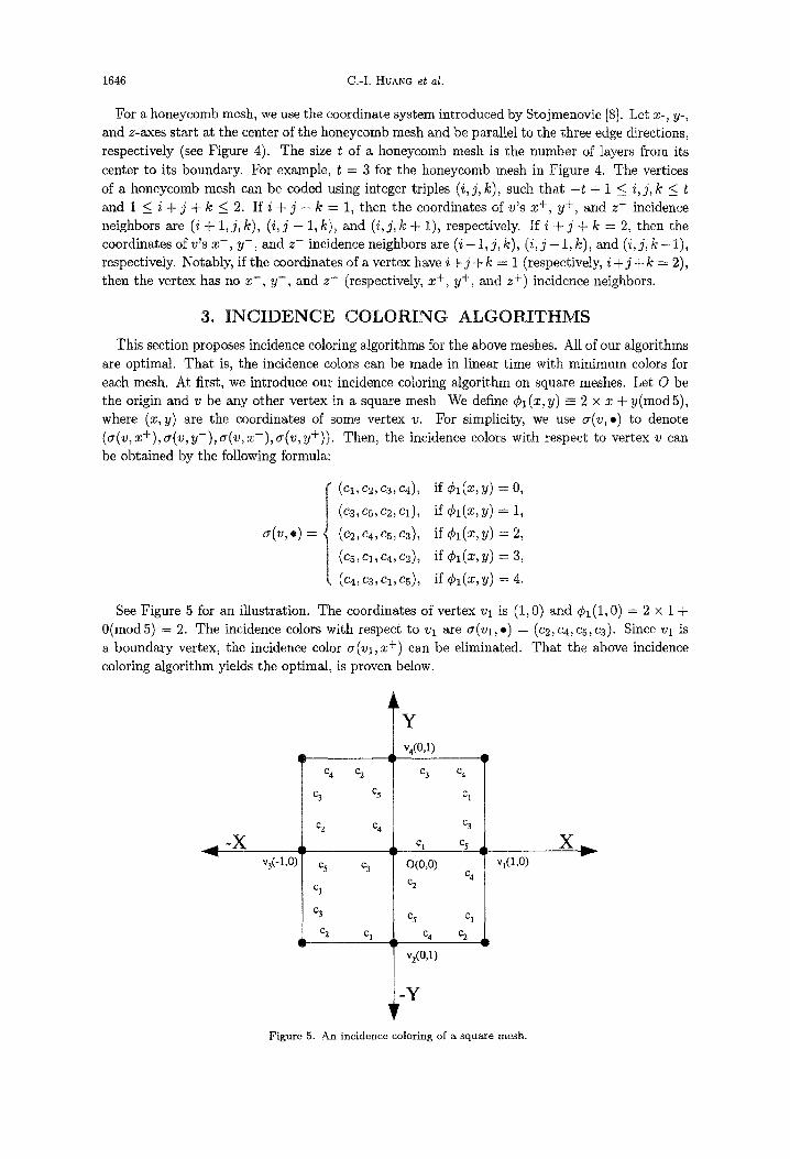
This section proposes incidence coloring algorithms for the above meshes. All of our algorithms are optimal. That is, the incidence colors can be made in linear time with minimum colors for each mesh. At first, we introduce our incidence coloring algorithm on square meshes. Let O be the origin and v be any other vertex in a square mesh. We define ¢1(x,y) -- 2 x x + y(mod5), where (x, y) are the coordinates of some vertex v. For simplicity, we use a(v, .) to denote (0"(% x+), a(v, y-) , ~r(v, x-) , a(v, y+)). Then, the incidence colors with respect to vertex v can be obtained by the following formula:

=o, (C3,C5,C2, Cl), if Ct(x ,y )= 1,

~(v,®)= (c2, ca,cs,c3), if Cz(x,y) =2 ,

(cs,cl,c4, c2), if Cx(x,y) =3 ,

(c4, c3,cl,cs), if Ca(x,y) =4 .

See Figure 5 for an illustration. The coordinates of vertex vl is (1, 0) and ¢t(1, 0) = 2 x 1 + 0(mod5) = 2. The incidence colors with respect to vl are ~(vl,e) = (c2,c4,c5,c3). Since Vl is a boundary vertex, the incidence color ¢(vl, x +) can be eliminated. That the above incidence coloring algorithm yields the optimal, is proven below.

_ , - X

c4 %

c 3 c5

C 2 C 4

V3(- 1 ,o)T 05 03

C 1

C 3

C2 C 1

Y v4(O,1)

C3 C4 i C 1

C 3 C I C S

O(0,0)%% c, c4 I vl(l'0)

C 4 C 2 v2(O,1)

Figure 5. An incidence coloring of a square mesh.

r

The Incidence Coloring Numbers 1647

THEOREM 1. Let G be a square mesh. Then, xi(G) = 5.

PROOF. Let v be any vertex in G with coordinates (p, q). We want to prove tha t the incidence colors with respect to v are satisfied with the coloring requirement, i.e., no two adjacent incidences have the same color. Since ¢1 (P, q) is between 0 and 4, there are fives cases to be considered. We only show tha t it is t rue for the case where ¢1 (P, q) = 0. The other cases can be handled similarly. The vertices adjacent to v are vl, v2, v3, and v4 whose coordinates are ( p + l , q), (p, q - l ) , ( p - l , q), and (p,q+ 1), respectively, (see Figure 5). If ¢I(P,q) = 0, then ¢ 1 ( P + 1,q) = 2, ¢l(P,q - 1) = 4,

¢1(P "- 1, q) = 3, and ¢1(P, q + 1) = 1. Thus, or(v1, *) = (c2, C4, C5, C3), O'(V2, O) = (C4, C3, el , c5) , cr(v3, . ) = (c5, cl, c4, c2), and e(v4, . ) = (c3, c5, c2, cl). Only the adjacent incidences of (v, x +) are considered. The adjacent incidences of other incidences can be handled similarly. The incidences adjacent to (v,x +) are (v ,x - ) , (v,y+), (v ,y-) , (vl,x+), (v l ,x - ) , (vl,y+), and (v l ,y - ) whose incidence colors are c3, c4, c2, c2, c5, c3, and c4, respectively. All of the incidence colors differ from cl which is the incidence color of (v, x+). Clearly, the proposed incidence coloring algorithm uses only five colors. Therefore, xi(G) = 5. |

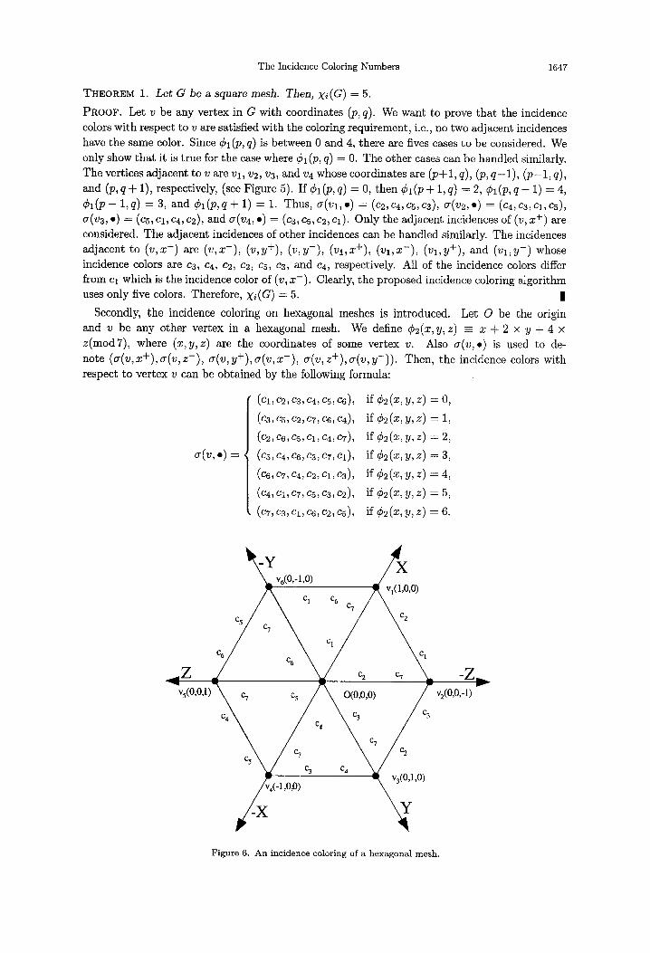
Secondly, the incidence coloring on hexagonal meshes is introduced. Let O be the origin and v be any other vertex in a hexagonal mesh. We define ¢2(x,y,z) - x + 2 x y + 4 x z(mod7) , where (x ,y ,z) axe the coordinates of some vertex v. Also or(v,.) is used to de- note (cr(v, x+), ~(v, z-) , a(v, y+), a(v, x - ) , ~(v, z+), a(v, y - ) ) . Then, the incidence colors with respect to ver tex v can be obtained by the following formula:

(cl,c2,c3,c4, c~,c6), if ¢2(x,

~(v,*) =

y,z) =o, (c3,c~,c2,c7, c6,c4), if ¢2(x,y,z) = 1,

(c2,c6,c~,cl,c4,c7), if ¢2(x,y,z) = 2,

(c5,c4, c6,c3,c7,cl), if ¢2(x,y,z) = 3,

(c6, c7, c4, c2,cl,c3), if ¢2 (x , y , z )=4 ,

(c4, cl,c7, c5,e3,c2), if C2(x,y,z) = 5,

(c~, c3, c1, c6, c2, eh), if ¢~(x,y,z) = 6.

c5

-y

C 1 C 6 C 7

v~(1,0,0)

vs(O,O,1)

c4k• c7 c5 o(0,0,0)

C3

v2(0,0,-1)

%

% c4

v,(-1,0,0)

, c 2

v3(O,l,O)

\ Y

Figure 6. An incidence coloring of a hexagonal mesh.

1648 c.-I. HUANG et al.

See Figure 6 for an illustration. The coordinates of vertex vl is (1,0, 0) and ¢2 (1,0, 0) = 1 + 2 × 0+ 4 x 0(mod 7) = 1. The incidence colors with respect to Vl are or(v1, . ) = (c3, c5, c2, c7, c6, c4). Since vl is a boundary vertex, the incidence colors ~r(vl,x+), cr(vl,z-) and cr(vl,y-) can be eliminated. Wi th a similar proof as Theorem 1, we can obtain the following theorem.

THEOREM 2. Let G be a hexagonal mesh. Then, Xi(G) = 7.

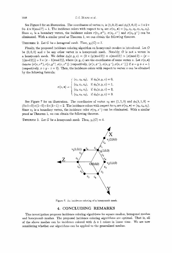
Finally, the proposed incidence coloring algorithm on honeycomb meshes is introduced. Let O be (0, 0, 0) and v be any other vertex in a honeycomb mesh. Notably, O is not a vertex in a honeycomb mesh. We define C3(x,y,z) = (2 x (y(mod2)) + z (mod2) ) x (x(mod2) - (x - l ( m o d 2))) + 3 × (x - l (mod2) ) , where (x,y, z) are the coordinates of some vertex v. Let ~r(v~ .) denote (~(v, x+), or(v, y+)~ cr(v~ z+)) (respectively, (a(v, x - ) , ~(v, y - ) , or(v, z - ) ) ) if x ÷ y + z = 1 (respectively, x + y q- z = 2). Then, the incidence colors with respect to ver tex v can be obtained by the following formula:

o ( v , , ) = (c3,c ,cl),

if ¢ 3 ( x , y , z ) = 0,

if ¢3 (z, y, z) = 1,

if Ca(x ,y , z) = 2,

if C3(x,y , z) = 3.

See Figure 7 for an illustration. The coordinates of vertex v2 are (1, 1, 0) and ¢3(1, 1,0) = (2× 1+0) x ( 1 - 0 ) + 3 × ( 1 - 1 ) = 2. The incidence colors with respect to v2 are a(v2, *) = (c3, c4, cl). Since v2 is a boundary vertex, the incidence color a(v2, z - ) can be eliminated. With a similar proof as Theorem 1, we can obtain the following theorem.

THEOREM 3. Let G be a honeycomb mesh. Then, x~(G) = 4.

4

,0,0)

V3(1,O,1 ) ~C4 C3 J cl

C 2 C 3 C 4

- v 2 ( 1 , 1 , O )

C4 / ~ 2 c3

C 3 C 4

Z

Figure 7. An incidence coloring of a honeycomb mesh.

4. C O N C L U D I N G R E M A R K S

This investigation proposes incidence coloring algorithms for square meshes, hexagonal meshes and honeycomb meshes. The proposed incidence coloring algorithms are optimal. Tha t is, all of the above meshes can be incidence colored with A -q- 1 colors in linear time. We are now considering whether our algorithms can be applied to the generalized meshes.

The Incidence Coloring Numbers 1649

R E F E R E N C E S 1. R.A. Brualdi and J.Q. Massey, Incidence and strong edge color graphs, Discrete Mathematics 122, 51-58,

(1993). 2. B. Guiduli, On incidence coloring and star arboricity of graphs, Discetet Mathematics 163, 275-278, (1997). 3. I. Algor and N. Alon, The star arboricity of graphs, Discrete Mathematics "/5, 11-22, (1989). 4. W.C. Shiu, P.C.B. Lam and D.L. Chen, On incidence coloring for some cubic graphs, Discrete Mathematics

252, 259-266, (2002). 5. V. Milutinovid, Mapping of neural networks on the honeycomb architectures, Proceedings of the IEEE 77

(12), 1875-1878, (1989). 6. M. Chen, K.G. Shin and D.D. Kandlur, Addressing, routing, and broadcasting in hexagonal mesh multipro-

cessors, IEEE Transactions on Computers 39 (1), 10-18, (1990). 7. F.G. Nocetti, I. Stojmenovic and J. Zhang, Addressing and routing in hexagonal networks with applications

for tracking mobile users and connection rerouting in cellular networks, IEEE Transactions on Parallel and Distributed Systems 13 (9), 963-971, (2002).

8. I. Stojmenovic, Honeycomb networks: Topological properties and communication algorithms, IEEE Trans- actions on Parallel and Distributed Systems 8 (10), 1036-1042, (1997).

9. J. Carle, J. Myoupo and D. Seine, All-to-all broadcasting algorithms on honeycomb networks and applications, Parallel Processing Letters 9 (4), 539-550, (1999).