THE IMPORTANCE OF LOW FREQUENCIES IN NOISE ANNOYANCE

Paul SchomerSchomer & Associates, Inc

2117 Robert Drive, Champaign, IL, 61821, USAPhone: 217 359 6602 Fax: 217 359-3303

e-mail: schomer@uiuc.edu

1. INTRODUCTION

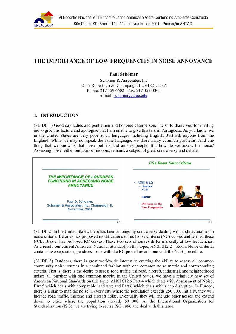
(SLIDE 1) Good day ladies and gentlemen and honored chairperson. I wish to thank you for invitingme to give this lecture and apologize that I am unable to give this talk in Portuguese. As you know, wein the United States are very poor at all languages including English. Just ask anyone from theEngland. While we may not speak the same language, we share many common problems. And onething that we know is that noise bothers and annoys people. But how do we assess the noise?Assessing noise, either outdoors or indoors, remains a subject of great controversy and debate.

(SLIDE 2) In the United States, there has been an ongoing controversy dealing with architectural roomnoise criteria. Beranek has proposed modifications to his Noise Criteria (NC) curves and termed theseNCB. Blazier has proposed RC curves. These two sets of curves differ markedly at low frequencies.As a result, our current American National Standard on this topic, ANSI S12.2—Room Noise Criteria,contains two separate appendices—one with the RC procedure and one with the NCB procedure.

(SLIDE 3) Outdoors, there is great worldwide interest in creating the ability to assess all commoncommunity noise sources in a combined fashion with one common noise metric and correspondingcriteria. That is, there is the desire to assess road traffic, railroad, aircraft, industrial, and neighborhoodnoises all together with one common metric. In the United States, we have a relatively new set ofAmerican National Standards on this topic, ANSI S12.9 Part 4 which deals with Assessment of Noise;Part 5 which deals with compatible land use; and Part 6 which deals with sleep disruption. In Europe,there is a plan to map the noise in every city where the population exceeds 250 000. Initially, they willinclude road traffic, railroad and aircraft noise. Eventually they will include other noises and extenddown to cities where the population exceeds 50 000. At the International Organization forStandardization (ISO), we are trying to revise ISO 1996 and deal with this issue.

2

(SLIDE 4) For years, many have suggested that A-weighting was inadequate for assessing combinednoise environments. In the famous Kryter-Schultz debate in JASA (1978, 1982), Kryter took issuewith Schultz and suggested that for the same A-weighted day-night sound level (DNL), aircraft noisewas more annoying than road traffic noise. Recently, in a paper in Noise Control Engineering Journal(1994), Finegold and von Gierke et al. from the United States suggest that there are indeed systematicdifferences in annoyance between aircraft, road traffic, and railroad noise for the same DNL, and theyoffer a set of curves to show these differences. In an even more recent paper in JASA, Miedema(1998) offers yet another set of curves that show differences between the annoyance generated byaircraft, road traffic, and railroad noise for the same DNL.

(SLIDE 5) In today’s talk, I suggest that the Beranek-Blazier controversy and the controversy overassessing combined environmental noise situations are really both part of the same issue. Noiseassessment, either indoors or outdoors, requires that we properly note and assess the low frequencycontent of the sound. Today, I will show that the methods of both Beranek and Blazier fail to properlyaccount for low frequency sound. When one does properly account for the low frequency sound, thenthe two methods merge together. For environment noise, I will show that much of the reporteddifferences between transportation noise sources are due to not properly assessing the contribution ofthe low frequency sound. In both cases, I will make use of the equal-loudness level contours found inISO 226-1987. Please note, I am not talking about loudness calculations as are given by researcherssuch as Zwicker or Stevens. My method does not use the loudness calculations of ISO 532. I amtalking about the pure tone measured equal-loudness level contours that are found in ISO 226.

(SLIDE 6) This lecture is based on 4 journal articles and 3 Internoise papers and the 5 listed on theslide are the main papers that contribute to this particular paper.

“Evaluation of Loudness-Level Weightings for Assessing the Annoyance of Environmental Noise,”draft submitted to Journal of the Acoustical Society of America, 2001.

“Use of the proposed new ISO 226 equal-loudness level contours as a filter to assess noise annoyance,”

3

INTERNOISE 2001, Institute of Noise Control Engineering International, Delft, The Netherlands, 27-30August 2001.

“A comparison between the use of loudness level weighting and loudness measures to assessenvironmental noise from combined sources,” INTERNOISE 2000, Paper No. 101, Institute of NoiseControl Engineering International, Nice, France, 27-30 August 2000.

“A test of proposed revisions to room noise criteria curves,” Noise Control Engineering Journal, 48(4),124-129, (July/August 2000).

“Proposed revisions to room noise criteria,” Noise Control Engineering Journal, 48(3), 85-96, (May/June2000).

“Loudness-Level Weighting for Environmental Noise Assessment,” Acustica and Acta Acustica, 86(1),49-61 (January/February 2000).

“On the use of loudness weighted sound levels to assess community noise,” INTERNOISE 1999,Institute of Noise Control Engineering International, Ft. Lauderdale, FL, USA, 6-8 December 1999.

I will deal first with the indoor, room noise criteria issues and then with the environmental noiseissues.

2. ASSESSING ROOM NOISE

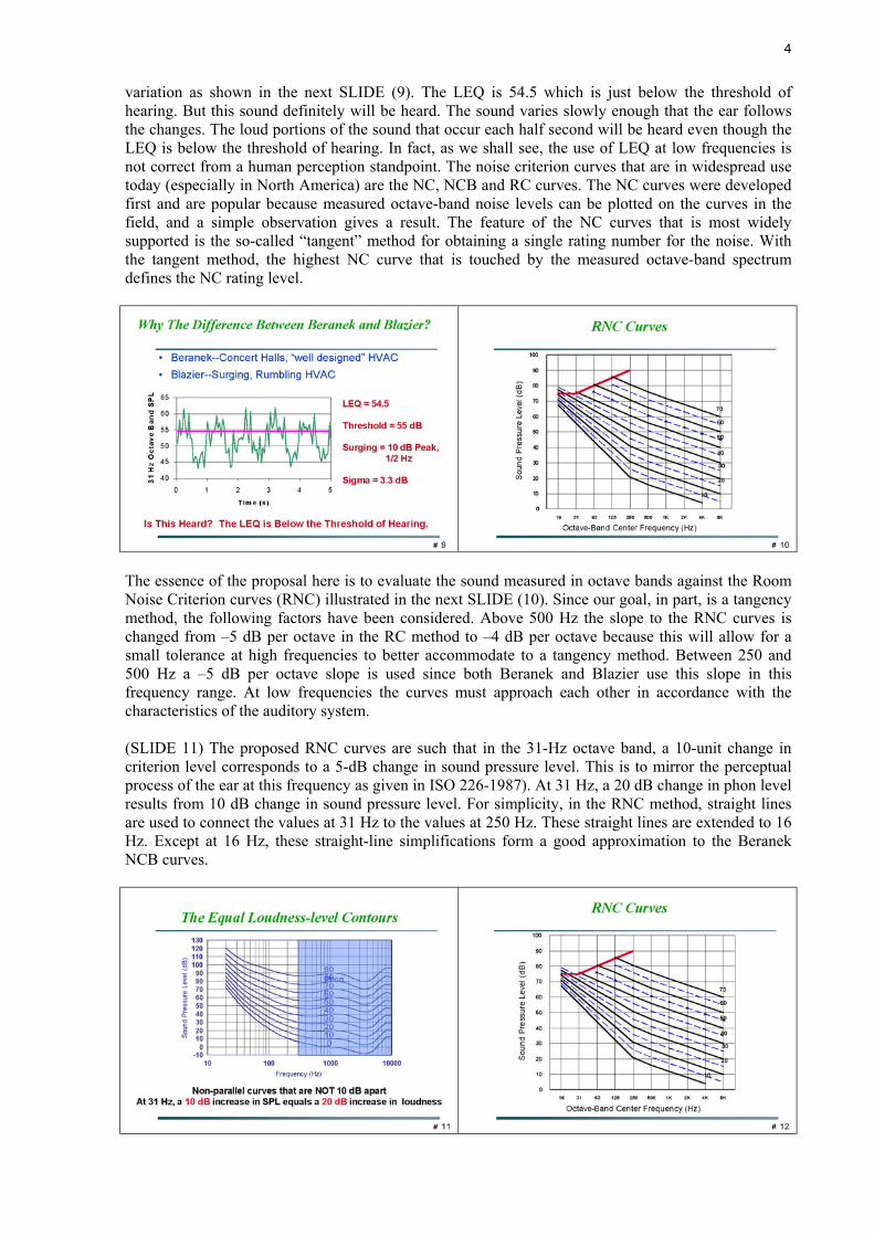
(SLIDE 7) The recent American National Standard, Criteria for Evaluating Room Noise, presents twosets of room noise criteria curves; one termed NCB and the other RC (ANSI, 1995). The NCBcriterion curves are given in this slide. Beranek (1997) derived these curves from the characteristics ofhearing to be consistent with equal loudness curves and to be consistent with subjective responses.The RC criterion curves are given in the next SLIDE (8).They are parallel lines with a –5 dB peroctave slope that goes through the stated RC value in the 1000 Hz octave band. Blazier (1981, 1997)derived these curves from experimental studies of noise in 68 offices where there were no complaints.The RC curves are designed to include the effects of slowly fluctuating low-frequency noise.

The two sets of room criterion curves each are based on data and theory, and each is correct for aspecific set of situations. These two sets of criterion curves depart most markedly from one another atlow frequencies and low sound levels. Also, each set has its problems. The RC curves set criterialevels that are below the threshold of hearing. This is done to protect against modern, energy efficientheating and ventilating (HVAC) systems that generate large turbulent fluctuations at low frequenciesand can include fan surging with concomitant noise level surging of 10 dB or more. On the other hand,the NCB curves set criteria levels that are based on “well-behaved” HVAC systems—systems whereturbulence generation is minimized and fan surging does not exist.

Note that the RC curves extend below the threshold of hearing. Is this a mistake? Consider sound inthe 31 Hz octave band that surges between two levels that are 10 dB apart and also has considerable

4

variation as shown in the next SLIDE (9). The LEQ is 54.5 which is just below the threshold ofhearing. But this sound definitely will be heard. The sound varies slowly enough that the ear followsthe changes. The loud portions of the sound that occur each half second will be heard even though theLEQ is below the threshold of hearing. In fact, as we shall see, the use of LEQ at low frequencies isnot correct from a human perception standpoint. The noise criterion curves that are in widespread usetoday (especially in North America) are the NC, NCB and RC curves. The NC curves were developedfirst and are popular because measured octave-band noise levels can be plotted on the curves in thefield, and a simple observation gives a result. The feature of the NC curves that is most widelysupported is the so-called “tangent” method for obtaining a single rating number for the noise. Withthe tangent method, the highest NC curve that is touched by the measured octave-band spectrumdefines the NC rating level.

The essence of the proposal here is to evaluate the sound measured in octave bands against the RoomNoise Criterion curves (RNC) illustrated in the next SLIDE (10). Since our goal, in part, is a tangencymethod, the following factors have been considered. Above 500 Hz the slope to the RNC curves ischanged from –5 dB per octave in the RC method to –4 dB per octave because this will allow for asmall tolerance at high frequencies to better accommodate to a tangency method. Between 250 and500 Hz a –5 dB per octave slope is used since both Beranek and Blazier use this slope in thisfrequency range. At low frequencies the curves must approach each other in accordance with thecharacteristics of the auditory system.

(SLIDE 11) The proposed RNC curves are such that in the 31-Hz octave band, a 10-unit change incriterion level corresponds to a 5-dB change in sound pressure level. This is to mirror the perceptualprocess of the ear at this frequency as given in ISO 226-1987). At 31 Hz, a 20 dB change in phon levelresults from 10 dB change in sound pressure level. For simplicity, in the RNC method, straight linesare used to connect the values at 31 Hz to the values at 250 Hz. These straight lines are extended to 16Hz. Except at 16 Hz, these straight-line simplifications form a good approximation to the BeranekNCB curves.

5

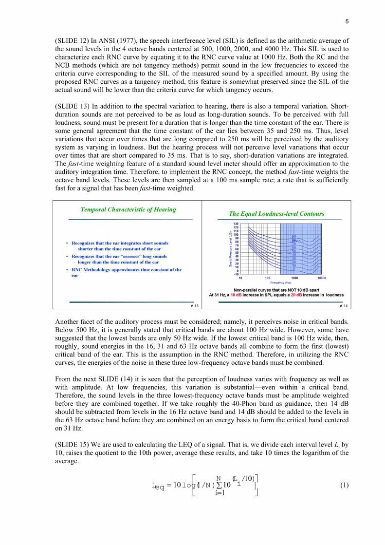
(SLIDE 12) In ANSI (1977), the speech interference level (SIL) is defined as the arithmetic average ofthe sound levels in the 4 octave bands centered at 500, 1000, 2000, and 4000 Hz. This SIL is used tocharacterize each RNC curve by equating it to the RNC curve value at 1000 Hz. Both the RC and theNCB methods (which are not tangency methods) permit sound in the low frequencies to exceed thecriteria curve corresponding to the SIL of the measured sound by a specified amount. By using theproposed RNC curves as a tangency method, this feature is somewhat preserved since the SIL of theactual sound will be lower than the criteria curve for which tangency occurs.

(SLIDE 13) In addition to the spectral variation to hearing, there is also a temporal variation. Short-duration sounds are not perceived to be as loud as long-duration sounds. To be perceived with fullloudness, sound must be present for a duration that is longer than the time constant of the ear. There issome general agreement that the time constant of the ear lies between 35 and 250 ms. Thus, levelvariations that occur over times that are long compared to 250 ms will be perceived by the auditorysystem as varying in loudness. But the hearing process will not perceive level variations that occurover times that are short compared to 35 ms. That is to say, short-duration variations are integrated.The fast-time weighting feature of a standard sound level meter should offer an approximation to theauditory integration time. Therefore, to implement the RNC concept, the method fast-time weights theoctave band levels. These levels are then sampled at a 100 ms sample rate; a rate that is sufficientlyfast for a signal that has been fast-time weighted.

Another facet of the auditory process must be considered; namely, it perceives noise in critical bands.Below 500 Hz, it is generally stated that critical bands are about 100 Hz wide. However, some havesuggested that the lowest bands are only 50 Hz wide. If the lowest critical band is 100 Hz wide, then,roughly, sound energies in the 16, 31 and 63 Hz octave bands all combine to form the first (lowest)critical band of the ear. This is the assumption in the RNC method. Therefore, in utilizing the RNCcurves, the energies of the noise in these three low-frequency octave bands must be combined.

From the next SLIDE (14) it is seen that the perception of loudness varies with frequency as well aswith amplitude. At low frequencies, this variation is substantial—even within a critical band.Therefore, the sound levels in the three lowest-frequency octave bands must be amplitude weightedbefore they are combined together. If we take roughly the 40-Phon band as guidance, then 14 dBshould be subtracted from levels in the 16 Hz octave band and 14 dB should be added to the levels inthe 63 Hz octave band before they are combined on an energy basis to form the critical band centeredon 31 Hz.

(SLIDE 15) We are used to calculating the LEQ of a signal. That is, we divide each interval level Li by10, raises the quotient to the 10th power, average these results, and take 10 times the logarithm of theaverage.

∑=

=N

iiL

NeqL1

1010110

)/()/(log (1)

6

But, this does not work for fluctuating noises at low frequencies. Consider a sequence of measurednoise intervals for which the levels in the 1 kHz band fluctuate as a square wave between 60 and 80dB at a 1-Hz rate. For one-half of a second the level is 60 dB and for the next one-half second it is 80dB. From the next SLIDE (16), we see that a sound pressure level of 60 dB at 1 kHz corresponds to aloudness level of 60 phons and 80 dB corresponds to 80 phons. The equivalent level of such a signal isabout 77 dB and from the slide, the loudness level is 77 phons. The LEQ is 17 dB above the lowerSPL, and the phon level also is 17 dB above the lower phon level.

Consider now the case of the same signal located in the 31 Hz octave band. Here, an SPL equal to 60dB corresponds to a loudness level of 10 phons. The LEQ is still 77 dB, but an increase of 17 dB inLEQ at 31 Hz from 60 dB corresponds to a loudness level increase of 32 phons. Here a 10-phonincrease in loudness results from approximately a 5 dB increase in SPL. The increase in loudness levelat 31 Hz is about double that of the same signal level at 1 kHz.

(SLIDE 17) Assume that for a certain octave frequency band, 10 phon steps in the loudness levelcurves are caused by changes in sound level of δ dB. The equation for calculating the “true” level,Leqδ, taking δ into account is shown in this slide.

δ

δ

δ

δ

Km

L

N

i

mL

iL

Nm

L

N

i

mL

mL

iL

NeqL

+=

∑=

−

+=

∑=

+−

=

1

10

))(/10(

10)/1(log10

1

10

))(/10(

10)/1(log10

(2)

It is apparent that if δ equals 10, then this equation reduces to the equation for LEQ as it should then Leqδ reduces to LEQ.

(SLIDE 18) In summary, for the development of an RNC evaluation one does the following. Each ofthese noise level packets is created from samples of the fast-time-weighted sound levels in threefrequency regions, (1) the 16, 31 and 63 Hz octave bands, (2) the 125 Hz band, and (3) the 250 Hz and

7

higher bands. For each 100 ms time sample, the three low frequency octave-band levels are combinedon an energy basis after diminishing the 16 Hz band by 14 dB and increasing the 63 Hz band by 14dB. Thus, a simple time series is created. This time series contains the level fluctuations over time inthe three low-frequency octave bands—the levels and fluctuations that the hearing process is sensitiveto. We are calculating a penalty or adjustment to add to the 31 Hz octave band that accounts for howthe ear is hearing and perceiving the sound. This adjustment is added to the 31 Hz octave band level.The adjustment that is added to the 31 Hz octave band level is just LL – LEQ. This adjusted 31 Hzoctave band is used in the RNC calculations. We also perform a similar calculation for the 125 Hzband but with δ=8. The adjusted octave band levels are then compared to the RNC curves using atangent method as shown in the next SLIDE (19). In this example, after adjustment, the octave banddata are tangent with a highest value of 70 RNC at 31 Hz. Worked examples using this procedure canbe found in the references.

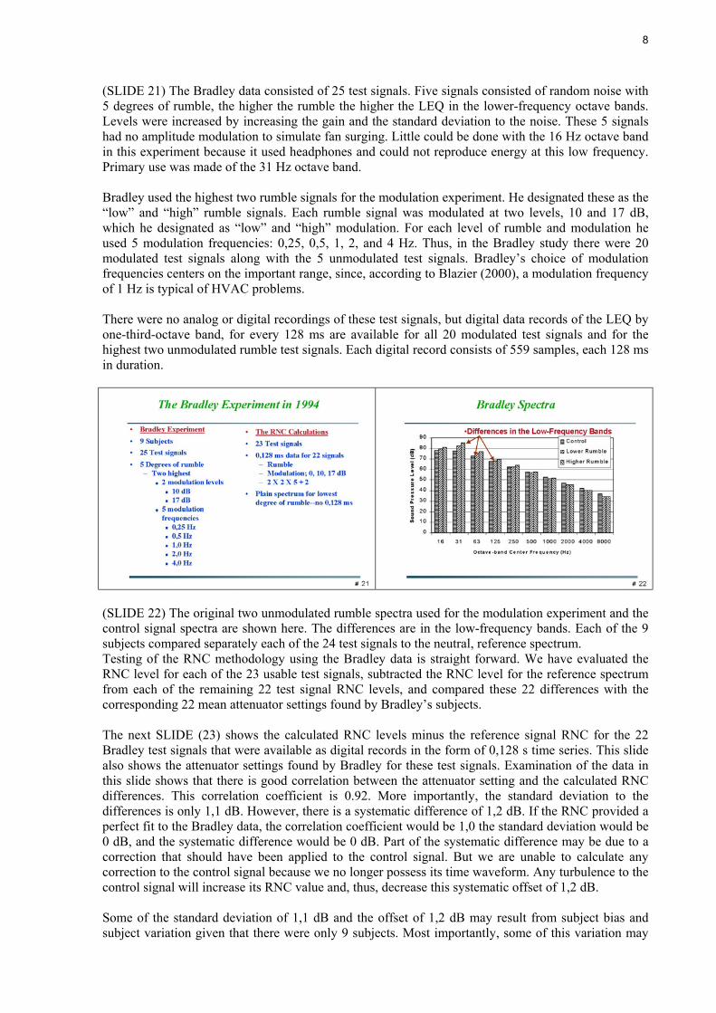
(SLIDE 20) We Now Show A Test of The RNC MethodBradley (1994) studied the annoyance generated in rooms by sounds that contain various degrees ofturbulence and surging at low frequencies. He reports on an initial experiment to evaluate theadditional annoyance caused by varying amounts of low-frequency rumble sounds from HVACsystems. HVAC noises were simulated with various levels of low-frequency sound and varyingamounts of amplitude modulation of the low-frequency components. Nine subjects listened to the testsounds over headphones and adjusted the level of the test sounds to be equally annoying as a fixedneutral reference sound. The neutral test sound was random noise with a minus 5 dB per octave slopeto the spectrum. Bradley used time-series of short-term LEQ levels to evaluate these sounds. Theshort-term LEQ levels were calculated each 128 ms for each one-third-octave band. Thus, these datacan be used to test the RNC methodology. The 128 ms LEQ levels certainly approximate a series offast-time-weighted levels, and the energies in the 16, 31, and 63 Hz octave bands can be combinedaccording the RNC methodology. The resulting RNC levels can be compared with the psycho-acoustical evaluations provided by Bradley’s subjects. We use the Bradley data to test the RNCmethodology.

8

(SLIDE 21) The Bradley data consisted of 25 test signals. Five signals consisted of random noise with5 degrees of rumble, the higher the rumble the higher the LEQ in the lower-frequency octave bands.Levels were increased by increasing the gain and the standard deviation to the noise. These 5 signalshad no amplitude modulation to simulate fan surging. Little could be done with the 16 Hz octave bandin this experiment because it used headphones and could not reproduce energy at this low frequency.Primary use was made of the 31 Hz octave band.

Bradley used the highest two rumble signals for the modulation experiment. He designated these as the“low” and “high” rumble signals. Each rumble signal was modulated at two levels, 10 and 17 dB,which he designated as “low” and “high” modulation. For each level of rumble and modulation heused 5 modulation frequencies: 0,25, 0,5, 1, 2, and 4 Hz. Thus, in the Bradley study there were 20modulated test signals along with the 5 unmodulated test signals. Bradley’s choice of modulationfrequencies centers on the important range, since, according to Blazier (2000), a modulation frequencyof 1 Hz is typical of HVAC problems.

There were no analog or digital recordings of these test signals, but digital data records of the LEQ byone-third-octave band, for every 128 ms are available for all 20 modulated test signals and for thehighest two unmodulated rumble test signals. Each digital record consists of 559 samples, each 128 msin duration.

(SLIDE 22) The original two unmodulated rumble spectra used for the modulation experiment and thecontrol signal spectra are shown here. The differences are in the low-frequency bands. Each of the 9subjects compared separately each of the 24 test signals to the neutral, reference spectrum.Testing of the RNC methodology using the Bradley data is straight forward. We have evaluated theRNC level for each of the 23 usable test signals, subtracted the RNC level for the reference spectrumfrom each of the remaining 22 test signal RNC levels, and compared these 22 differences with thecorresponding 22 mean attenuator settings found by Bradley’s subjects.

The next SLIDE (23) shows the calculated RNC levels minus the reference signal RNC for the 22Bradley test signals that were available as digital records in the form of 0,128 s time series. This slidealso shows the attenuator settings found by Bradley for these test signals. Examination of the data inthis slide shows that there is good correlation between the attenuator setting and the calculated RNCdifferences. This correlation coefficient is 0.92. More importantly, the standard deviation to thedifferences is only 1,1 dB. However, there is a systematic difference of 1,2 dB. If the RNC provided aperfect fit to the Bradley data, the correlation coefficient would be 1,0 the standard deviation would be0 dB, and the systematic difference would be 0 dB. Part of the systematic difference may be due to acorrection that should have been applied to the control signal. But we are unable to calculate anycorrection to the control signal because we no longer possess its time waveform. Any turbulence to thecontrol signal will increase its RNC value and, thus, decrease this systematic offset of 1,2 dB.

Some of the standard deviation of 1,1 dB and the offset of 1,2 dB may result from subject bias andsubject variation given that there were only 9 subjects. Most importantly, some of this variation may

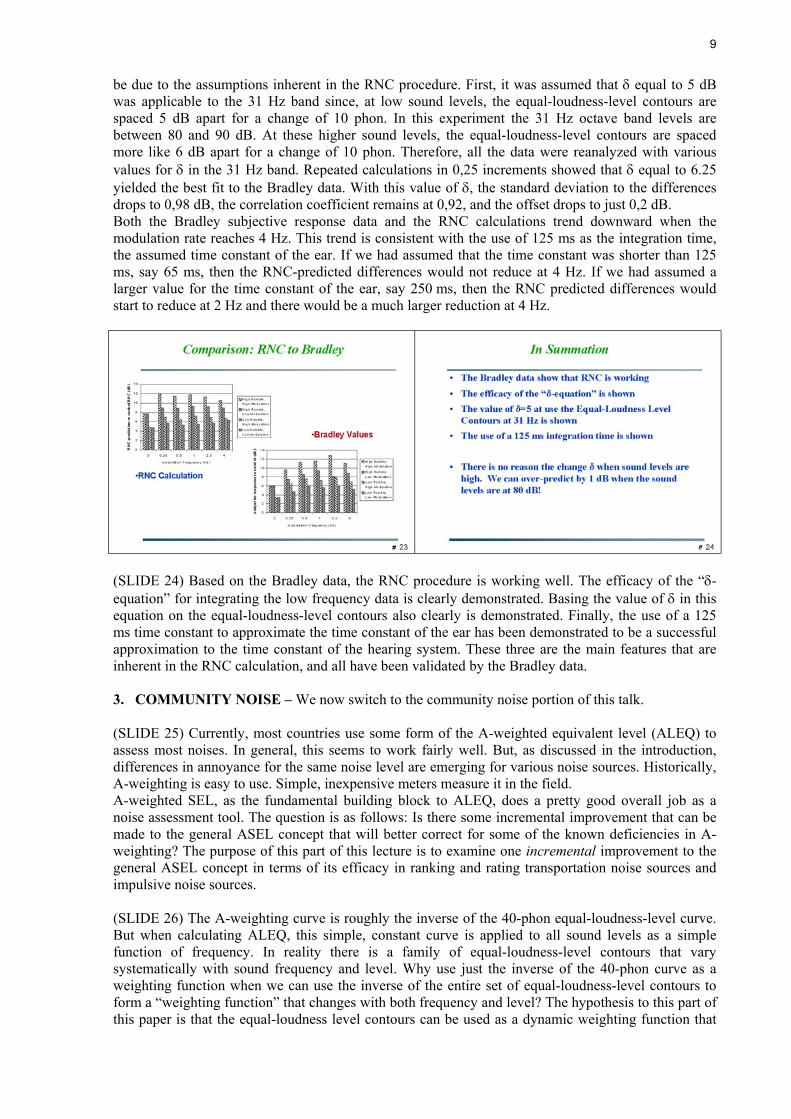
9

be due to the assumptions inherent in the RNC procedure. First, it was assumed that δ equal to 5 dBwas applicable to the 31 Hz band since, at low sound levels, the equal-loudness-level contours arespaced 5 dB apart for a change of 10 phon. In this experiment the 31 Hz octave band levels arebetween 80 and 90 dB. At these higher sound levels, the equal-loudness-level contours are spacedmore like 6 dB apart for a change of 10 phon. Therefore, all the data were reanalyzed with variousvalues for δ in the 31 Hz band. Repeated calculations in 0,25 increments showed that δ equal to 6.25yielded the best fit to the Bradley data. With this value of δ, the standard deviation to the differencesdrops to 0,98 dB, the correlation coefficient remains at 0,92, and the offset drops to just 0,2 dB.Both the Bradley subjective response data and the RNC calculations trend downward when themodulation rate reaches 4 Hz. This trend is consistent with the use of 125 ms as the integration time,the assumed time constant of the ear. If we had assumed that the time constant was shorter than 125ms, say 65 ms, then the RNC-predicted differences would not reduce at 4 Hz. If we had assumed alarger value for the time constant of the ear, say 250 ms, then the RNC predicted differences wouldstart to reduce at 2 Hz and there would be a much larger reduction at 4 Hz.

(SLIDE 24) Based on the Bradley data, the RNC procedure is working well. The efficacy of the “δ-equation” for integrating the low frequency data is clearly demonstrated. Basing the value of δ in thisequation on the equal-loudness-level contours also clearly is demonstrated. Finally, the use of a 125ms time constant to approximate the time constant of the ear has been demonstrated to be a successfulapproximation to the time constant of the hearing system. These three are the main features that areinherent in the RNC calculation, and all have been validated by the Bradley data.

3. COMMUNITY NOISE – We now switch to the community noise portion of this talk.

(SLIDE 25) Currently, most countries use some form of the A-weighted equivalent level (ALEQ) toassess most noises. In general, this seems to work fairly well. But, as discussed in the introduction,differences in annoyance for the same noise level are emerging for various noise sources. Historically,A-weighting is easy to use. Simple, inexpensive meters measure it in the field.A-weighted SEL, as the fundamental building block to ALEQ, does a pretty good overall job as anoise assessment tool. The question is as follows: Is there some incremental improvement that can bemade to the general ASEL concept that will better correct for some of the known deficiencies in A-weighting? The purpose of this part of this lecture is to examine one incremental improvement to thegeneral ASEL concept in terms of its efficacy in ranking and rating transportation noise sources andimpulsive noise sources.

(SLIDE 26) The A-weighting curve is roughly the inverse of the 40-phon equal-loudness-level curve.But when calculating ALEQ, this simple, constant curve is applied to all sound levels as a simplefunction of frequency. In reality there is a family of equal-loudness-level contours that varysystematically with sound frequency and level. Why use just the inverse of the 40-phon curve as aweighting function when we can use the inverse of the entire set of equal-loudness-level contours toform a “weighting function” that changes with both frequency and level? The hypothesis to this part ofthis paper is that the equal-loudness level contours can be used as a dynamic weighting function that

10

varies with frequency and level. This loudness-level weighting is an incremental change over A-weighting that improves the correlation with annoyance judgements. The general concept of SEL andLEQ calculated from a “filtering” is retained. For this paper, this hypothesis is tested againsttransportation and impulsive noise sources.

(SLIDE 27) This paper concentrates in an incremental change to the use of ASEL and ALEQ. Itcreates loudness-level weighted SEL that is designated LLSEL and loudness-level-weighted LEQ thatis designated LL-LEQ. These metrics retain the log-base-10 energy summation process inherent inASEL. In contrast, the methods of loudness per ISO 532b depart from the log-base-10 energysummation process. The methods of loudness use a log-base-2 summation process, so the methods ofloudness represent a much further departure from the concepts of ASEL and ALEQ than do theconcepts given in this paper where we retain the log-base 10 summation. The philosophy of this paperis that ASEL and ALEQ work fairly well. The energy addition inherent in these A-weighted measuresshould be retained; only an incremental improvement is required.

(SLIDE 28) Equal-loudness-level contours are given in functional form in ISO 226 [19]. The functionsin ISO 226 correspond to one-third octave band center frequencies from 20 Hz to 12500 Hz.Conceptually, the analysis proceeds from a one-third-octave-band spectral analysis using the equal-loudness-level contours. Each one-third-octave-band sound pressure level (SPL) is assigned the phonlevel that corresponds to that frequency and level.

(SLIDE 29) As with the RNC procedure, the fast-time weighting is used to approximate the timeconstant of the ear. But here, one-third octave bands are used for the analysis. That is, the output of aone-third-octave-band spectrum analyzer can be set to fast-integration time. The spectrum is sampledevery 100 ms.

(SLIDE 30) This time-series of 100 ms, one-third-octave-band spectra is used to calculate the overalltime- and frequency-summed phon level, LL, as is shown in the slide:

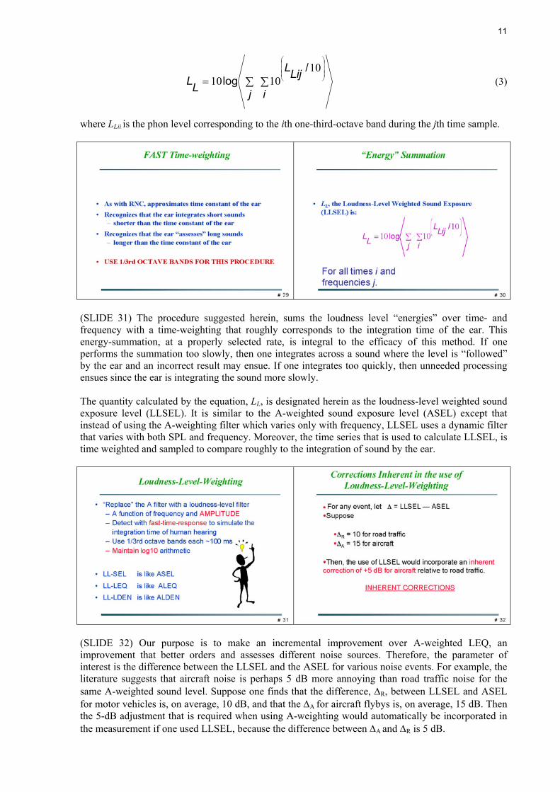
11

∑∑=

i

LijL

jLL

101010

/log (3)

where LLii is the phon level corresponding to the ith one-third-octave band during the jth time sample.

(SLIDE 31) The procedure suggested herein, sums the loudness level “energies” over time- andfrequency with a time-weighting that roughly corresponds to the integration time of the ear. Thisenergy-summation, at a properly selected rate, is integral to the efficacy of this method. If oneperforms the summation too slowly, then one integrates across a sound where the level is “followed”by the ear and an incorrect result may ensue. If one integrates too quickly, then unneeded processingensues since the ear is integrating the sound more slowly.

The quantity calculated by the equation, LL, is designated herein as the loudness-level weighted soundexposure level (LLSEL). It is similar to the A-weighted sound exposure level (ASEL) except thatinstead of using the A-weighting filter which varies only with frequency, LLSEL uses a dynamic filterthat varies with both SPL and frequency. Moreover, the time series that is used to calculate LLSEL, istime weighted and sampled to compare roughly to the integration of sound by the ear.

(SLIDE 32) Our purpose is to make an incremental improvement over A-weighted LEQ, animprovement that better orders and assesses different noise sources. Therefore, the parameter ofinterest is the difference between the LLSEL and the ASEL for various noise events. For example, theliterature suggests that aircraft noise is perhaps 5 dB more annoying than road traffic noise for thesame A-weighted sound level. Suppose one finds that the difference, ∆R, between LLSEL and ASELfor motor vehicles is, on average, 10 dB, and that the ∆A for aircraft flybys is, on average, 15 dB. Thenthe 5-dB adjustment that is required when using A-weighting would automatically be incorporated inthe measurement if one used LLSEL, because the difference between ∆A and ∆R is 5 dB.

12

(SLIDE 33) As discussed above, the calculation of LLSEL must be performed on a 100-ms time seriesof fast-time-weighted one-third-octave-band spectra. Therefore, evaluation of the difference betweenLLSEL and ASEL requires the real-time or recorded time-history of the event. From previous researchprojects (Schomer, 1994, 1995), time-history tape recordings were available for the following:

• A variety of road vehicles driving past a fixed measurement location.• Helicopters flying past a fixed measurement location.• A variety of small and medium guns firing at various distances from a fixed measurement

location.

These data have been augmented by real-time measurements of motor vehicles on streets andhighways, aircraft taking off, aircraft landing, and electric and diesel train passbys. All of these datahave been analyzed to calculate the LLSEL, the ASEL, and the difference between these two. Theanalysis has been performed exactly as described above. The one-third-octave-band spectral timehistories were sampled every 100 ms after first detecting the one-third octave-band sound pressurelevels using the fast-integration time of the sound level meter. The equation shown a few slides ago,with the coefficients from ISO 226, was used to find the phon level corresponding to each such one-third-octave-band sound pressure level. These phon levels were summed on an energy basis to find theLLSEL. At each time interval, the analyzer also provided the A-weighted level. This time-series offast-time-weighted, A-weighted levels was summed on an energy basis to find the ASEL. Theselevels, so calculated, are reported in this paper.

(SLIDE 34) Studies at Munster in Germany (Schomer, 1994) and studies at Aberdeen Proving Ground(abbreviated APG) in the United States (Schomer, 1995) both used the passby sound of motor vehiclesas a control sound for paired-comparison testing with gunfire and other military equipment. The motorvehicles ranged from small (e.g., a van) to large (e.g., a tank transport). Supplemental measurementswere made on streets and by interstate highways in Champaign, Illinois, and by an interstate highwaynear Seattle, Washington.

(SLIDE 35) Fixed-wing aircraft data were gathered near the “SeaTac” airport which is situatedbetween Seattle and Tacoma, Washington, USA. Measurements were made under the flight tracks atdistances between 5 and 12 km from touchdown (on landing) or start of roll (on takeoff), so, at leaston landing, the distance of closest approach was about 250 to 600 m.The APG study also included a “Huey” UH-1H helicopter that flew by the site at constant speed at analtitude of about 100 m over a heavily treed area. There were two ground distances from the studyhouse to the flight-track projection on the ground. These were designated “near” and “far” distances.

(SLIDE 36) Train data were gathered at APG which is situated along side the train tracks that run fromNew York City, to Philadelphia, to Baltimore, and on to Washington DC. This is the busiest passengertrain corridor in the USA having about 4 passbys per hour, and these trains are electric in contrast todiesel trains that are more common in the USA. There were also a couple of slow-moving, short dieselfreight trains that were measured. There were three conditions: electric trains at constant high speed(perhaps 120 km/h), electric trains slowing for a nearby station stop, and slow, short diesel freight

13

trains. The distance from the tracks to the measurements was about 150 m.

(SLIDE 37) The general relationship for ∆i found among the transportation noise sources fits the dataprovided by Finegold (1994) and the general trends provided by Miedema (1995). The Finegold et al.and Miedema data show aircraft noise to be more annoying than road traffic noise and, in general, the∆A for aircraft is greater than the ∆R for road traffic. In fact, the numerical results fit the Finegold et.al. data quite well. In the slide, the adjustment for aircraft relative to road traffic grows with DNL fromperhaps 0 at 50 DNL to about 5 at 70 DNL. At typical community noise levels (50 to 70 DNL), theadjustment averages perhaps 2-3 dB. In this same range, there is a positive difference or no differencefor trains relative to road traffic. We will call the difference zero since at higher DNLs the differencebetween trains and road traffic is negative. The Miedema data show greater differences as comparedwith the Finegold et. al. data, but the trends are the same. The differences in ∆i found herein also fitthe trends in the Miedema data.

(SLIDE 38) Gunfire was a part of the Munster and APG studies. In the Munster study, the NATO G-3rifle was used firing blank ammunition; in the APG study, the M-16 rifle was used firing serviceammunition. The APG test also included the Bradly Fighting Vehicle 25-mm cannon. Both theMunster and the APG studies used exactly the same test protocol and the control vehicles describedabove. The results indicated that penalties of about 16, 12, or 8 dB are required to properly assess the25-mm cannon, M-16 rifle, and NATO G-3 rifle, respectively. So the penalty for the 25-mm cannonwas 4 dB greater than the penalty for the M-16 rifle which in turn was 4 dB greater than the penaltyfor the G-3 rifle. The ASEL and LLSEL have been analyzed for a sample of these three weapons, and,on average, ∆GG3 equals 1,9, ∆GM16 equals 5,2, and ∆G25mm equals 8,9.

The difference in (A-weighted) penalty between the 25-mm cannon and the M16 of 4 dB equals thedifference in ∆G between these two. Also, the (A-weighted) difference in penalty between the M-16and the G-3 of 4 dB almost equals the difference in ∆G of 3 dB between these two. The use of LLSELwould correctly order these three highly impulsive sources and would automatically include the

14

correct relative numerical adjustments required when using A-weighting.

(SLIDE 39) The transportation and gunfire data can be listed in one table. For this analysis weconsider traffic noise to have an A-weighted adjustment of zero when assessed using ASEL and/orALEQ. All other sources are plotted with adjustments to their A-weighted levels that are relative to theA-weighted levels for traffic noise. For example, the NATO G3 rifle fire sound is given an adjustmentof 8 dB based on Schomer (1994). All of the adjustments are listed in the slide. As noted, the valuesfor the transportation noise source adjustments are based primarily on Finegold et al.

The next SLIDE (40) plots the data from the previous slide. It contains transportation noise sourcedata (circles), gunfire noise date (stars) and gunfire data shifted by 12 dB (squares). This slide alsocontains the “ideal” relation that is a dashed line with slope of one that goes through the point (0,5).The line goes through this point because our reference sound, traffic noise, had an A-weightedadjustment of 0 and a value of ∆R equal to 5. This figure shows that if transportation noises areassessed using LLSEL, then a consistent framework is established since the data fit the ideal relationalmost perfectly. There is a separate consistent framework for gunfire noise since the slope of therelation between corrections to A-weighting and ∆G values is one. However, the relation for gunfirenoise sources does not coincide with the relation for transportation noise sources. Rather, they areparallel lines that are separated by 12 dB. In order to make all 6 noise sources fit one relation it isnecessary to add an adjustment of 12 phon to all calculations or measurements of the phon level forgunfire.

(SLIDE 41) A new version of ISO 226 has been proposed and is currently under ballot as a DraftInternational Standard. The following analysis compare computations of LLSEL using the currentmethod and the proposed new method. The proposed new equal-loudness level contours give muchless emphasis to the low frequencies than do the present contours.

(SLIDE 42) This slide shows that calculations using the current ISO 226 (blue squares) correlate well

15

with the subjective A-weighted adjustments but that calculations using the newly proposed ISO 226(red circles) virtually do not correlate with the subjective adjustments. In this slide, the gunfire dataform one nearly horizontal line and the vehicle data form another nearly horizontal line. Without the12-dB impulse noise adjustment, all of the data using the proposed ISO 226 curves forms onehorizontal line that is absolutely independent of the subjective adjustments.(SLIDE 43) The problem with the proposed ISO 226 curves is that, at the low frequencies, they yield asubstantially lower phon level for the same sound pressure level. The slide compares the phon levelcalculated in each 1/3rd-octave band when the sound level in each band is 60 dB. The current ISO 226curves yield substantially higher phon levels in the lower frequency bands.

(SLIDE 44) This slide shows the (energy) time-integrated phon levels in each 1/3rd-octave band usingboth the current and the proposed ISO 226 curves for a helicopter fly by. The current procedure showsmuch higher phon levels at low frequencies—40 dB higher in some bands. The overall LLSEL also isshown. This difference is more than 10 dB.

(SLIDE 45) The next slide shows a similar comparison for small arms gunfire. The previous 3 slidesshow that there is a big difference in the emphasis that the two sets of curves place on the lowfrequency energies. The current ISO 226 places a greater emphasis on the low frequency energies and,in terms of annoyance, it correlates very much better with subjective human response.

4. IN CONCLUSION

(SLIDE 46) The concepts inherent in the equal-loudness level contours can be used to effectivelydescribe peoples’ responses, indoors, to room noise and to explain the differences between criteriaproposed by Beranek and Blazier. Date gathered earlier by Bradley confirm the efficacy of thismethod. The concepts inherent in the equal-loudness level contours can be used to effectively describepeoples’ response, outdoors, to environmental noise. Loudness-level-weighted sound exposure level(LLSEL) and loudness-level-weighted equivalent level (LL-LEQ) can be used to assess environmental

16

noise. Compared with A-weighting, loudness-level weighting will better order and assesstransportation noise sources, and it will better assess sounds with strong, low-frequency content. Also,with the addition of a 12-dB adjustment, loudness-level weighting will better order and assess highlyimpulsive sounds.

Since Type 1, hand-held one-third-octave-band instruments are readily available at relatively lowcosts, it would be inexpensive to implement LLSEL and LL-LEQ and room noise criteria capabilitiesin these hand-held instruments. Thus, significant improvements can be made to the measurement andassessment of environmental noise without resorting to the large number of adjustments that arerequired when assessing sound using the A-weighting.

The LLSEL calculated using the current ISO 226 curves does a much better job of assessing combinednoise sources as compared with calculations using the proposed new ISO 226 curves. The difference isthe emphasis that the two sets of curves place on the low-frequency energies. The current ISO 226places a much greater emphasis on the low frequency energies and, in terms of annoyance, it correlatesvery much better with subjective human response.

This result clearly shows the importance of properly assessing the contribution of the low-frequencysound energies to noise annoyance. The differences in annoyance judgements between sources appearto mainly stem from their low-frequency energy content. Any method to assess combined noiseenvironments or indoor room noise criteria should take these differences in low-frequency energycontent into account. LEQ is not a proper measurement of low frequency noise. It fails to take intoaccount the characteristics of hearing. Sounds with LEQs below the threshold of hearing may be veryaudible. A modified LEQ function that takes into account the spacing of the equal-loudness-levelcontours is required.

(SLIDE 47) My recommendation is that we not use A-weighting to assess low-frequency noise. Wemust use the loudness function, probably, as given by the current ISO 226. We must use somethinglike fast-time weighting to account for the time constant of hearing. These assessment procedures canall easily be built into a simple hand-held instrument that costs less than $6000. In large quantities, thecost would be much less than $6000.

17

5. REFERENCES

American National Standards Institute (ANSI) (1995). American National Standard Criteria forEvaluating Room Noise, ANSI S12.2-1995, Acoustical Society of America, New York, NY.

Beranek, Leo, (1997). “Applications of NCB and RC noise criterion curves for specification andevaluation of noise in buildings,” Noise Control Eng. J., 45(5), 209-216, (September-October1997).

Bradley, John, (1994). “Annoyance caused by constant-amplitude and amplitude-modulated soundscontaining rumble,” Noise Control Eng. J., 42(6), 203-208 (November-December 1994).

Blazier, Warren, (1981). “Revised noise criteria for application in the acoustical design and rating ofHVAC systems,” Noise Control Eng. J., 16(2), 64-73 (March-April 1981).

Blazier, Warren, (1997). “RC Mark II; a refined procedure for rating the noise of heating, ventilatingand air-conditioning (HVAC) systems in buildings,” Noise Control Eng. J., 16(3), 64-73(November-December 1997).

Blazier, Warren, (2000). Personnel communications.

Finegold, L.S. and Harris, S.C. and von Gierke, H.E., (1994). “Community annoyance and sleepdisturbance: Updated criteria for assessing the impacts of general transportation noise on people.”Noise Control Eng. J., 42(1), 25-30, (January-February 1994).

Kryter, K.D., (1982). “Community annoyance from aircraft and ground vehicle noise,” J. Acoust. Soc.Am.. 72(2), 1222-1242, (October 1982).

Miedema, H.M.E., (1995). “Exposure-response relationships for transportation noise,” J. Acoust. Soc.Am., 104(6), 3432-3445, (December 1998).

Schomer, P.D. and Wagner, L.R. and Benson, L.J. and Buchta, E. and Hirsch, K.W. and Krahé, D.,(1994). “Human and community response to military sounds: Results from field-laboratory testsof sounds of small arms, tracked-vehicle, and blast sounds,” Noise Control Eng. J., 42(2), 71-84,(March-April 1994).

Schomer, P.D. and Wagner, L.R., (1995). “Human and community response to military sounds—Part2: Results from field-laboratory tests of sounds of small arms, 25-mm cannons, helicopters, andblasts,” Noise Control Eng. J, 43(1), 1-13, (January-February 1995).

Schultz, T.J. (1978). “Synthesis of social surveys on noise annoyance,” J. Acoust. Soc. Am. 64(2), 377-405, (August 1978).

Schultz, T.J., (1982). “Comments on K.D. Kryter’s paper: Community annoyance from aircraft andground vehicle noise,” J. Acoust. Soc. Am., 72(2), 1243-1252, (October 1982).