The Importance of Environmental Factors inForecasting Australian Power Demand

Ali Eshragh∗ Benjamin Ganim† Terry Perkins‡ Kasun Bandara§

Abstract

We develop a time series model to forecast weekly peak power demand for threemain states of Australia for a yearly time-scale, and show the crucial role of envi-ronmental factors in improving the forecasts. More precisely, we construct a seasonalautoregressive integrated moving average (SARIMA) model and reinforce it by employ-ing the exogenous environmental variables including, maximum temperature, minimumtemperature, and solar exposure. The estimated hybrid SARIMA-regression model ex-hibits an excellent mean absolute percentage error (MAPE) of 3.41%. Moreover, ouranalysis demonstrates the importance of the environmental factors by showing a re-markable improvement of 46.3% in MAPE for the hybrid model over the crude SARIMA

model which merely includes the power demand variables. In order to illustrate theefficacy of our model, we compare our outcome with the state-of-the-art machine learn-ing methods in forecasting. The results reveal that our model outperforms the latterapproach.

1 Introduction

Electrical energy is a vital resource to drive industries [26]. Thus, energy demand forecastingis essential to the economic and socioeconomic aspects of modern society. Accurate forecastsensure that utilities can meet energy demand and avoid undesirable events in the networksuch as black-outs and load shedding. While underestimation is undesirable, overestimationleads to wasted resources. In spite of recent advances in storage technologies, demandforecasting models are still critical in power planning [9].

In general, there are four main time-scales (or, forecast horizons) for power demandmodeling [11]:

∗School of Information and Physical Sciences, University of Newcastle, NSW, Australia, and InternationalComputer Science Institute, Berkeley, CA, USA. Email: ali.eshragh@newcastle.edu.au

†School of Information and Physical Sciences, University of Newcastle, NSW, Australia. Email:Benjamin.Ganim@uon.edu.au

‡School of Information and Physical Sciences, University of Newcastle, NSW, Australia. Email:Terry.Perkins@uon.edu.au

§School of Computing and Information Systems, Melbourne Centre for Data Science, University of Mel-bourne, VIC, Australia. Email: Kasun.Bandara@unimelb.edu.au

1

arX

iv:1

911.

0081

7v3

[st

at.A

P] 3

0 O

ct 2

021

(i) Long-term load forecasting (LTLF) is used for expansion planning of the network;(ii) Medium-term load forecasting (MTLF) is used for operational planning;(iii) Short-term load forecasting (STLF) is used for day to day planning and dispatch costminimization;(iv) Very short-term load forecasting (VSTLF) on the scale of seconds to minutes allows thenetwork to respond to the flow of demand.

Australia is a vast and environmentally diverse continent with climate zones rangingfrom equatorial to temperate. It is thus important to understand how the dynamics ofpower demand varies across different regions.

In this paper, we develop a seasonal autoregressive integrated moving average (SARIMA)model to forecast peak weekly demand in the medium-term (i.e., MTLF). The demand dataare from three main Australian states consisting of: New South Wales (NSW), Victoria(VIC), and South Australia (SA). To investigate the impact of the environmental factors onthe power demand, we hybridize the SARIMA model with a linear regression model by em-ploying the exogenous environmental variables including, maximum temperature, minimumtemperature, and solar exposure. Our results reveal that the latter hybrid model improvesthe accuracy of forecasts by an average factor of 46.3% over the three states. Furthermore,to demonstrate the efficacy of the hybrid model, its outputs are compared with the state-of-the-art machine learning methods in forecasting. The results reveal that the former hybridmodel outperforms the latter methods.

The structure of this paper is organized as follows: Section 2 provides a review of theliterature and establishes the motivation for using a SARIMA-regression model. Section 3 dis-cusses the data resources and aggregation, and visualizes the obtained time series. Section4 explains the details of the statistical procedure to fit a SARIMA model to the weekly peakpower demand data. In Section 5, we employ secondary environmental time series to con-struct a hybrid SARIMA-regression model. Section 6 discusses the quality of 52-week forecastsand compare the outcome with the state-of-the-art machine learning methods in forecasting.Finally, Section 7 presents a final discussion of our findings, and provides conclusions anddirections for future research.

2 Literature Review and Motivation

Energy demand is an amalgamation of millions of individual demand requirements fromconsumers, varying with time, weather, population growth, electricity price and many othereconomic factors (e.g., see [28] and [19]). The time dependency of the demand along with itsinherent seasonality to weather patterns across a yearly time-scale would suggest time seriesmethods to study the dynamics of the demand.

Box and Jenkins [8] introduced their celebrated SARIMA model for analyzing those non-stationary time series displaying seasonal effects in their behavior. Each SARIMA model is alinearly transformed time series constructed by differencing the original time series at properlags. A hybrid SARIMA-regression approach could be effective, if the time covariance of theseries is well captured by the SARIMA component and the remaining mean value of trends is

2

captured by the exogenous independent variables (e.g., see [1,9]). Although it has been morethan 40 years since such model were developed, due to their simplicity and vast practicality,they continue to be widely used in theory and practice, particularly effectively in electricitydemand forecasting.

Crude SARIMA as well as hybrid SARIMA-regression models have formed the basis of manypower forecasting models with a focus on STLF to MTLF time-scale (i.e., looking days toweeks ahead) in several countries, as Nigeria [21], Iraq [19], Malaysia [22], South Africa [9],and Thailand [18]. Focusing on a metric of peak demand ensures that demand can be metwhen the electricity network is under maximum duress. Ghalehkhondabi et al. [10] studiedthe peak monthly demand in Northern India by using two different time series methodsincluding “SARIMA” and “exponential smoothing” models. The authors showed that theSARIMA model outperformed the exponential smoothing model on their data. In Australia,Amaral et al. [2] developed a smooth transition periodic autoregressive model for the NewSouth Wales power demand, and As’ad [3] predicted the peak demand for New South Walesat a daily resolution. For a more comprehensive overview of such techniques in power demandmodeling and forecasting, see [10].

In time series forecasting, global forecasting methods (GFM) that simultaneously learnsfrom a collection of time series, are becoming a strong alternative to the state-of-the-artunivariate statistical forecasting method such as SARIMA [6, 25]. In GFMs, a unified modelis built using a set of related time series that enables the model to exploit key structures,behaviors, and patterns common within a group of time series. In fact, more recently, deeplearning based GFMs have shown promising results in forecasting competitions and real-world applications (e.g., see [6, 13,14,23,25]).

While artificial neural networks (ANN) are increasing in popularity, Kandananond [18]compared ANN, multiple linear regression (MLR) and SARIMA models for electricity demandforecasting in Thailand. Although, they did not find a statistically significant differencebetween the three methods, MLR and SARIMA were simpler to compute, and the coefficientswere more easily interpreted.

In this paper, we develop a hybrid SARIMA-regression model to forecast the weekly peakpower demand in Australia over an MTLF time-scale, that is one year horizon (52 weeks).The main contribution of this work is to demonstrate the crucial role of novel environmentalvariables in the dynamics of the demand. The quality of forecasts are compared with thestate-of-the-art machine learning techniques. The results show that our model not onlyoutperforms the others, but also can more easily be computed and interpreted.

We conclude this section by noting that as electricity energy is still difficult to store, itis critical that the system can meet peak demand [28]. To the best of our knowledge, thiswork is the first attempt to investigate the impact of environmental factors on predictingthe aggregated weekly peak demand in an MTLF time-scale study.

3

3 Data: Resources, Aggregation and Visualizing

The power demand data for three major states of Australia, consisting of New South Wales(NSW), Victoria (VIC), and South Australia (SA), are obtained from the Australian EnergyMarket Operator [4]. They are measured in megawatts (MW). The secondary environmentaltime series data are acquired from the Australian Bureau of Meteorology [5]. We use thedata from those weather stations in close proximity to the primary population center foreach state. These major population centers are Sydney, Melbourne, and Adelaide for NSW,VIC, and SA, respectively. Table 1 lists the details of those weather stations.

Table 1: Australian Bureau of Meteorology weather stations

State Site BoM Site Number

NSW Sydney Airport 066037VIC Melbourne Airport 086282SA Brisbane Weather Station 040913

While the power demand data are given at 15-minute intervals, the environmental dataare recorded weekly. So the former are aggregated by finding the peak demand for each dayand then aggregating on a weekly basis. This aggregated value will be referred to as theweekly peak demand (WPD). The weekly data from the first week of January 2011 to thelast week of December 2016 (i.e., six years) are used as the training data for modeling andestimating the parameters. Following the MTLF time-scale, the data from the first week ofJanuary 2017 to the last week of December 2017 (i.e., 52 weeks) are used as the test data tocheck the accuracy of forecasts generated by the model.

The three secondary environmental time series used in this work are “maximum tem-perature”, “minimum temperature”, and “solar exposure”, denoted by Mint, Maxt and Solt,respectively. Solar exposure is defined as the amount of solar energy falling on a flat onemeter square surface, parallel to the ground and exposed to direct sunlight.

Figure 1 displays the time series of WPD from 2014 to 2016 (inclusive). Previous yearsshow similar seasonal trends. Visual inspection of these graphs reveals that the seasonaltrends may vary between the states.

Remark 1. All data analysis and graphing are conducted in R using the packages“astsa”a, “forecast” b, and “tseries”c, .

acran.r-project.org/web/packages/astsa/index.htmlbcran.r-project.org/web/packages/forecast/index.htmlccran.r-project.org/web/packages/tseries/index.html

4

Figure 1: Time series of the aggregated WPD for NSW, VIC, and SA over all of the trainingdata. For brevity and clarity other graphs in this report will only show the last three yearsof training data.

4 Crude SARIMA Model: WPD Time Series

We start this section by introducing a formal definition of a SARIMA model.

Definition 1 ( [24]). A time-series {xt; t = 0, 1, . . .} isSARIMA(p, d, q)× (P,D,Q)S, if

ΦP

(BS)φ(B)∇D

S∇dxt = δ + ΘQ

(BS)θ(B)wt,

where {wt; t = 0, 1, . . .} is a Gaussian white noise series, B is the backshift operator

5

(i.e., Bkxt = xt−k), and

φ(B) = 1− φ1B − φ2B2 − · · · − φpB

p,

ΦP

(BS)

= 1− Φ1BS − Φ2B

2S − · · · − ΦPBPS,

θ(B) = 1 + θ1B + θ2B2 + · · ·+ θqB

q,

ΘQ

(BS)

= 1 + Θ1BS + Θ2B

2S + · · ·+ ΘQBQS,

∇d = (1−B)d,

∇DS = (1−BS)D.

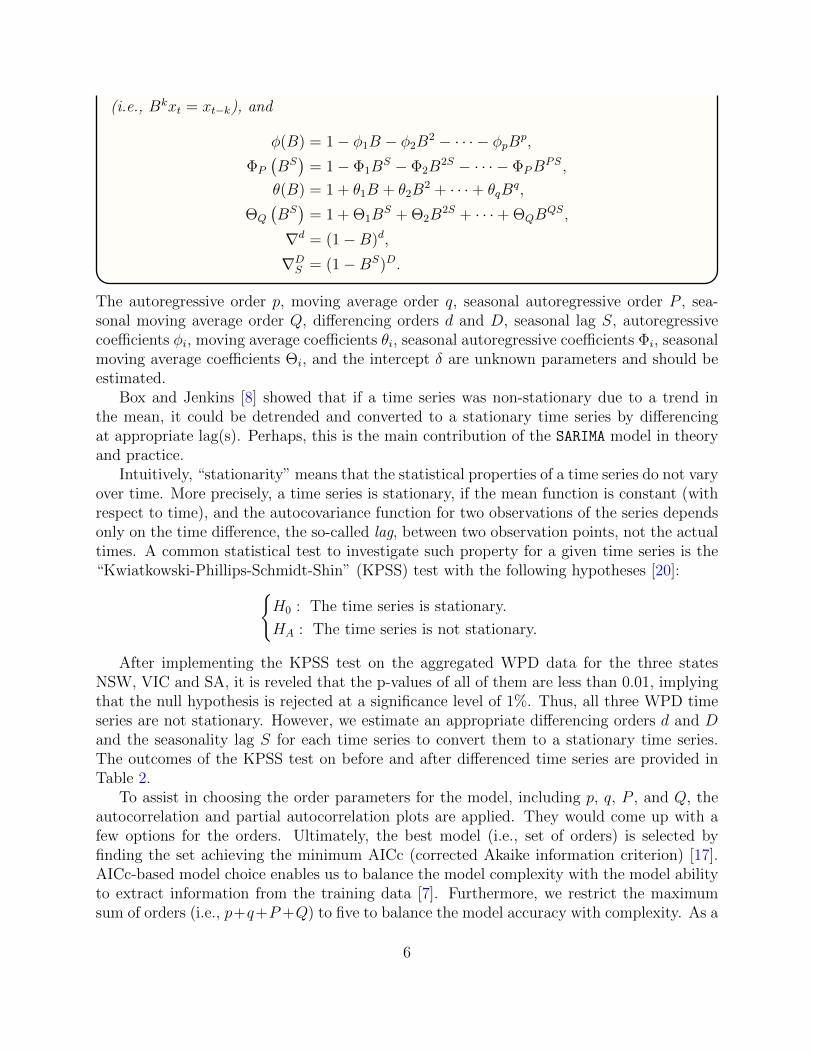
The autoregressive order p, moving average order q, seasonal autoregressive order P , sea-sonal moving average order Q, differencing orders d and D, seasonal lag S, autoregressivecoefficients φi, moving average coefficients θi, seasonal autoregressive coefficients Φi, seasonalmoving average coefficients Θi, and the intercept δ are unknown parameters and should beestimated.

Box and Jenkins [8] showed that if a time series was non-stationary due to a trend inthe mean, it could be detrended and converted to a stationary time series by differencingat appropriate lag(s). Perhaps, this is the main contribution of the SARIMA model in theoryand practice.

Intuitively, “stationarity” means that the statistical properties of a time series do not varyover time. More precisely, a time series is stationary, if the mean function is constant (withrespect to time), and the autocovariance function for two observations of the series dependsonly on the time difference, the so-called lag, between two observation points, not the actualtimes. A common statistical test to investigate such property for a given time series is the“Kwiatkowski-Phillips-Schmidt-Shin” (KPSS) test with the following hypotheses [20]:{

H0 : The time series is stationary.

HA : The time series is not stationary.

After implementing the KPSS test on the aggregated WPD data for the three statesNSW, VIC and SA, it is reveled that the p-values of all of them are less than 0.01, implyingthat the null hypothesis is rejected at a significance level of 1%. Thus, all three WPD timeseries are not stationary. However, we estimate an appropriate differencing orders d and Dand the seasonality lag S for each time series to convert them to a stationary time series.The outcomes of the KPSS test on before and after differenced time series are provided inTable 2.

To assist in choosing the order parameters for the model, including p, q, P , and Q, theautocorrelation and partial autocorrelation plots are applied. They would come up with afew options for the orders. Ultimately, the best model (i.e., set of orders) is selected byfinding the set achieving the minimum AICc (corrected Akaike information criterion) [17].AICc-based model choice enables us to balance the model complexity with the model abilityto extract information from the training data [7]. Furthermore, we restrict the maximumsum of orders (i.e., p+q+P+Q) to five to balance the model accuracy with complexity. As a

6

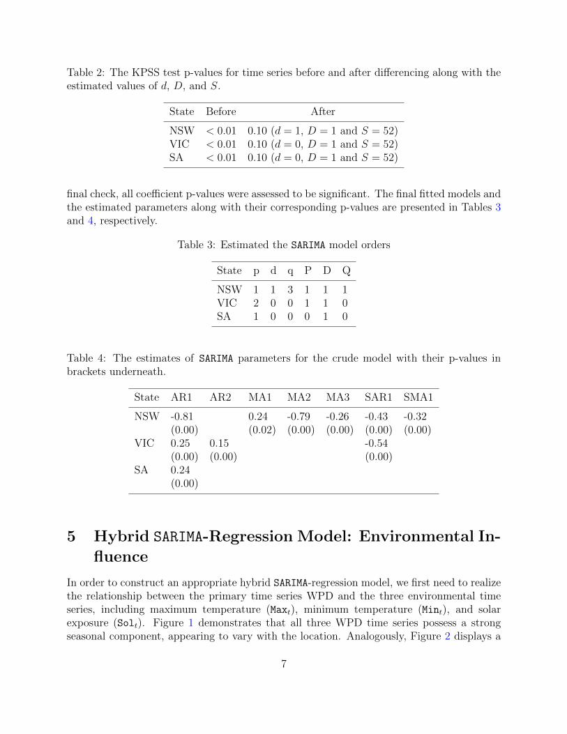
Table 2: The KPSS test p-values for time series before and after differencing along with theestimated values of d, D, and S.

State Before After

NSW < 0.01 0.10 (d = 1, D = 1 and S = 52)VIC < 0.01 0.10 (d = 0, D = 1 and S = 52)SA < 0.01 0.10 (d = 0, D = 1 and S = 52)

final check, all coefficient p-values were assessed to be significant. The final fitted models andthe estimated parameters along with their corresponding p-values are presented in Tables 3and 4, respectively.

Table 3: Estimated the SARIMA model orders

State p d q P D Q

NSW 1 1 3 1 1 1VIC 2 0 0 1 1 0SA 1 0 0 0 1 0

Table 4: The estimates of SARIMA parameters for the crude model with their p-values inbrackets underneath.

State AR1 AR2 MA1 MA2 MA3 SAR1 SMA1

NSW -0.81(0.00)

0.24(0.02)

-0.79(0.00)

-0.26(0.00)

-0.43(0.00)

-0.32(0.00)

VIC 0.25(0.00)

0.15(0.00)

-0.54(0.00)

SA 0.24(0.00)

5 Hybrid SARIMA-Regression Model: Environmental In-

fluence

In order to construct an appropriate hybrid SARIMA-regression model, we first need to realizethe relationship between the primary time series WPD and the three environmental timeseries, including maximum temperature (Maxt), minimum temperature (Mint), and solarexposure (Solt). Figure 1 demonstrates that all three WPD time series possess a strongseasonal component, appearing to vary with the location. Analogously, Figure 2 displays a

7

similar temporal and spatial variation for the secondary environmental time series (to savespace, only the NSW environmental time series are displayed). This observation implies thatthere could potentially be a significant relationship between the primary and secondary timeseries.

Figure 2: Maximum temperature, minimum temperature and solar exposure time series forNSW from 2014 to 2016 (inclusive)

Since the inference theory for the hybrid SARIMA-regression models with stationary re-gressor variables is completely different form that with non-stationarity variables, we needto test the stationarity of the environmental time series data at the outset. Therefore, theKPSS test is implemented on them and the corresponding p-values are reported in Table5. This table indicates that all three environmental time series over the three states arestationary at a significance level of 1%. Indeed, this outcome is visually supported by Figure2.

To investigate possible relationships between these exogenous environmental time seriesand the primary WPD time series, scatter plots are utilized. Figure 3 displays the scatterplots for NSW. This figure suggests that while the maximum and minimum temperatureshave a strong quadratic relationship with the WPD data, such relationship may not be as

8

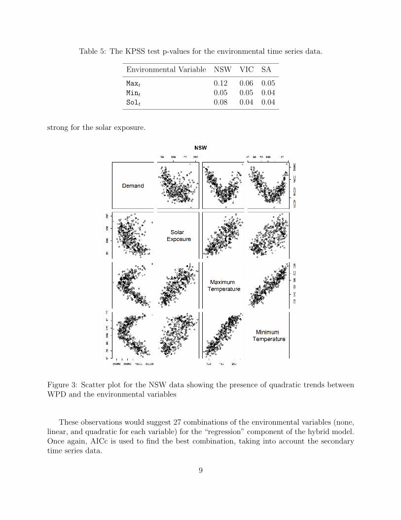
Table 5: The KPSS test p-values for the environmental time series data.

Environmental Variable NSW VIC SA

Maxt 0.12 0.06 0.05Mint 0.05 0.05 0.04Solt 0.08 0.04 0.04

strong for the solar exposure.

Figure 3: Scatter plot for the NSW data showing the presence of quadratic trends betweenWPD and the environmental variables

These observations would suggest 27 combinations of the environmental variables (none,linear, and quadratic for each variable) for the “regression” component of the hybrid model.Once again, AICc is used to find the best combination, taking into account the secondarytime series data.

9

The significance of each coefficient of the AICc chosen model was assessed and the finalselected combinations are presented in Table 6. This table shows that, while NSW andVIC require the full group of regression variables, surprisingly, SA does not seem to obtainsufficient benefit from the solar exposure time series. The estimates of model parameterswith their corresponding p-values are presented in Tables 7 and 8.

Table 6: Selected combination of environmental variables based on the minimum value ofAICc for each state

State Schematic structure of the regression component

NSW Maxt + Max2t + Mint + Min2t + Solt + Sol2tVIC Maxt + Max2t + Mint + Min2t + Solt + Sol2tSA Maxt + Max2t + Mint + Min2t

Table 7: The estimates of SARIMA parameters for the hybrid model with their p-values inbrackets underneath.

State AR1 AR2 MA1 MA2 SAR1 SMA1

NSW -0.90(0.00)

0.16(0.07)

-0.74(0.00)

-0.54(0.00)

VIC 0.48(0.00)

0.30(0.00)

-0.46(0.00)

SA 0.39(0.00)

0.13(0.03)

Table 8: The estimates of regression parameters for the hybrid model with their p-values inbrackets underneath (coefficients are rounded to one decimal places for brevity).

State Maxt Max2t Mint Min2t Solt Sol2t

NSW -770.8(0.00)

2.4(0.00)

-497.3(0.00)

2.6(0.00)

-61.6(0.03)

0.27(0.01)

VIC -328.2(0.00)

1.2(0.00)

-167.7(0.00)

1.2(0.00)

-83.6(0.00)

0.3(0.00)

SA -156.3(0.00)

0.5(0.00)

-82.7(0.00)

0.5(0.00)

Model Validation. The estimated models are checked for statistical validity by analyzingthe residuals. Figure 4 shows the autocorrelation function (ACF) as well as QQ-plot for the

10

residuals from the fitted hybrid SARIMA-regression model to the NSW WPD data. Clearly,the residuals have no autocorrelation at any lag, and the vast majority of the QQ-plot lieswell within the 95% significance area (i.e., shaded gray). Similar results are observed for theother two states.

Figure 4: ACF and QQ plots for the residuals from the fitted hybrid SARIMA-regression modelfor NSW

11

6 Medium-term Load Forecasting

The two crude SARIMA and hybrid SARIMA-regression models constructed in Sections 4 and5 are used to predict the WPD for all three states over 52 weeks in 2017. The resultsare displayed in Figure 5. In this figure, the black, red, blue and green plots are actualdemands, forecasts generated by the SARIMA model, forecasts generated by the SARIMA-regression model, and the 99% confidence boundary for WPD, respectively.

It is readily seen that the SARIMA-regression model performs significantly better than theSARIMA model. A more solid comparison can be carried out by finding the following twopopular measures to assess the effectiveness of the forecasts.

Definition 2 ( [27]). The mean absolute error (MAE) is defined as:

MAE =

∑ht=1 | ft − xt |

h,

where ft, xt and h are the forecast values, actual values, and prediction horizon, respec-tively. Analogously, the mean absolute percentage error (MAPE) is given by

MAPE =

∑ht=1

∣∣∣ft−xt

xt

∣∣∣h

× 100%.

Tables 9 and 10 display MAE and MAPE for the two estimated models and show thepercentage improvement by employing the exogenous environmental time series into themodel. The MAE and MAPE suggest an average 46.6% and 46.3% improvement in theaccuracy of forecasts when the environmental factors are included in the model, respectively.These observations highly support the importance of environmental factors in forecastingAustralian peak power demand.

Table 9: Comparison of MAE for the SARIMA and SARIMA-regression models

State SARIMA SARIMA-regression Improvement (%)

NSW 3962 1643 58.5VIC 2225 1372 38.3SA 885 504 43.0

Machine learning approach. In order to compare the performance of our proposedmodels with other methods, we apply the state-of-the-art machine learning approach toforecast WPD. More precisely, we use Recurrent Neural Networks (RNN) based GFM pro-posed by [12]. Table 12 summarises the optimal hyper-parameter values used in our exper-iments. According to [12], these optimal hyper-parameters are determined by a sequential

12

Figure 5: Comparison of the forecasts for the SARIMA and SARIMA-regression models to theactual WPD data for 2017

model-based algorithm configuration (SMAC), a variant of Bayesian Optimisation proposedby [15]. Furthermore, this framework uses COntinuous COin Betting (COCOB) optimisationalgorithm proposed by [16] that does not require tuning of the network learning rate.

13

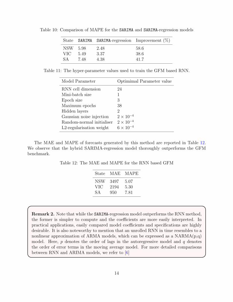
Table 10: Comparison of MAPE for the SARIMA and SARIMA-regression models

State SARIMA SARIMA-regression Improvement (%)

NSW 5.98 2.48 58.6VIC 5.49 3.37 38.6SA 7.48 4.38 41.7

Table 11: The hyper-parameter values used to train the GFM based RNN.

Model Parameter Optimimal Parameter value

RNN cell dimension 24Mini-batch size 1Epoch size 3Maximum epochs 38Hidden layers 2Gaussian noise injection 2× 10−4

Random-normal initialiser 2× 10−4

L2-regularisation weight 6× 10−4

The MAE and MAPE of forecasts generated by this method are reported in Table 12.We observe that the hybrid SARIMA-regression model thoroughly outperforms the GFMbenchmark.

Table 12: The MAE and MAPE for the RNN based GFM

State MAE MAPE

NSW 3497 5.07VIC 2194 5.30SA 950 7.81

Remark 2. Note that while the SARIMA-regression model outperforms the RNN method,the former is simpler to compute and the coefficients are more easily interpreted. Inpractical applications, easily compared model coefficients and specifications are highlydesirable. It is also noteworthy to mention that an unrolled RNN in time resembles to anonlinear approximation of ARMA models, which can be expressed as a NARMA(p,q)model. Here, p denotes the order of lags in the autoregressive model and q denotesthe order of error terms in the moving average model. For more detailed comparisonsbetween RNN and ARIMA models, we refer to [6]

14

7 Discussion and Conclusion

To the best of our knowledge, this work is the first attempt to investigate the crucial role ofenvironmental factors in the dynamics of the Australian electricity power demand. More pre-cisely, we developed a SARIMA-regression model for the weekly power demand in three majorstates of Australia, and empirically demonstrated the significant influence of environmentalfactors on predictions over a medium-term load forecasting time-scale (i.e., 52 weeks). Theresults revealed that while the SARIMA-regression model generated, on average, an MAPE of3.41% over all states, the environmental factors could improve the accuracy of forecasts bya factor of 46.3%. Such an excellent MAPE is comparable with the other methods listed inSection 2. However, a direct comparison might not be fair (in favor of our model) due to thelack of other MTLF studies in the literature of Australian weekly peak power demand. Thishighlights the potential explanatory influence and impact environmental variables may haveon power demand. Furthermore, we compared our model with the state-of-the-art machinelearning methods in forecasting and demonstrate the superiority of the former model.

The weather regression variables used within this work are historical data and providedwithout forecasting. This was done to maximise the predictive value of the regressors tohighlight their importance to predicting power demand. To move the model towards practicaluse future work could forecast the weather variables and use the predictions for the SARIMAregression. While this is expected to reduce the accuracy of the prediction, observationshows the weather variables are strongly seasonal and stationary and so should maintain themajority of their predictive power.

An alternative to using environmental data derived from a single weather station wouldbe to take the data from several sites across each state with different characteristics, and thenuse a weighted average by population. This method may help decision makers to identifya trend in demand that could improve the modeling of WPD. A practical drawback of thismethod is that many weather stations do not report complete data. Hence, the regressionsystem will have to adjust the missing values which may bring more errors into the model.

Our model provides a scaffold for future work in improving the accuracy and utility offorecasts. Incorporating additional environmental explanatory factors such as humidity andwind direction/strength could further improve the model and, consequently, the accuracy offorecasts.

References

[1] Abolghasemi, M., Hurley, J., Eshragh, A., and Fahimnia, B., Demand forecasting inthe presence of systematic events: Cases in capturing sales promotions, InternationalJournal of Production Economics, 230:107892, 2020.

[2] Amaral, L.F., Souza, R.C., and Stevenson, M., A smooth transition periodic autore-gressive (STPAR) model for short-term load forecasting, International Journal of Fore-casting, 24(4):603-615, 2008.

15

[3] As’ad, M., Finding the best ARIMA model to forecast daily peak electricity demand,Proceedings of the Fifth Annual ASEARC Conerence, University of Wollongong, 2012.

[4] Australian Energy Market Operator, www.aemo.com.au/Electricity/

National-Electricity-Market-NEM/Data-dashboard#aggregated-data.

[5] Australian Bureau of Meteorology, www.bom.gov.au/climate/data.

[6] Bandara, K., Bergmeir, C., and Smyl, S., Forecasting across time series databases usingrecurrent neural networks on groups of similar series: A clustering approach,ExpertSystems with Applications, 140:112896, 2020.

[7] Boroojeni, K. G., Amini, M. H., Bahrami, S., Iyengar, S. S., Sarwat, A. I., and Karaba-soglu, O., A novel multi-time-scale modeling for electric power demand forecasting:From short-term to medium-term horizon, Electric Power Systems Research, 142, 58-73, 2017.

[8] Box, G.E.P., Jenkins, G.M., Reinsel, G.C., and Ljung, G.M., Time series analysis:Forecasting and control, Wiley, 2015.

[9] Chikobvu, D., and Sigauke, C. Regression-SARIMA modelling of daily peak electricitydemand in South Africa, Journal of Energy in South Africa, 23(3):23-30, 2012.

[10] Ghalehkhondabi, I., Ardjmand, E., Weckman, G.R., and Young, W.A., An overviewof energy demand forecasting methods published in 2005-2015, Energy Systems, 2017.

[11] Hernandez, L., Baladron, C., Aguiar, J.M., Carro, B., Sanchez-Esguevillas, A.J.,Lloret, J., and Massana, J., A survey on electric power demand forecasting: Futuretrends in smart grids, microgrids and smart buildings, IEEE Communications Surveysand Tutorials, 16(3):1460-1495, 2014.

[12] Hewamalage, H. , Bergmeir, C., and Bandara, K., Recurrent neural networks for timeseries forecasting: Current status and future directions, International Journal of Fore-casting, 2020.

[13] Bandara, K., Bergmeir, C. and Hewamalage, H., LSTM-MSNet: Leveraging Forecastson Sets of Related Time Series With Multiple Seasonal Patterns, IEEE Trans NeuralNetw Learn Syst, Apr. 2020, doi: 10.1109/TNNLS.2020.2985720.

[14] Bandara, K., Bergmeir, C., Campbell, S., Scott, D. and Lubman, D., Towards AccuratePredictions and Causal ‘What-if’ Analyses for Planning and Policy-making: A CaseStudy in Emergency Medical Services Demand, presented at the International JointConference on Neural Networks, Glasgow, 2020.

[15] Hutter, F., Hoos, H.H., and Leyton-Brown, K., Sequential Model-based Optimizationfor General Algorithm Configuration, in Proceedings of the 5th International Confer-ence on Learning and Intelligent Optimization, Rome, Italy, 2011, pp. 507-523.

16

[16] Orabona, F. and Tommasi, T., Training Deep Networks Without Learning RatesThrough Coin Betting, in Proceedings of the 31st International Conference on NeuralInformation Processing Systems, Long Beach, California, USA, 2017, pp. 2157-2167

[17] Hurvich, C. M., and Tsai, C.-L., Regression and time series model selection in smallsamples, Biometrika, 76(2):297, 1989.

[18] Kandananond, K., Forecasting electricity demand in Thailand with an artificial neuralnetwork approach, Energies, 4:1246-1257, 2011.

[19] Kareem, Y.H., and Majeed, A.R., Sulaimany Governorate Using SARIMA, Building,(April 2003):1-5, 2006.

[20] Kwiatkowski, D., Phillips, P.C.B., Schmidt, P., and Shin, Y., Testing the null hypoth-esis of stationarity against the alternative of a unit root, Journal of Econometrics,54(1-3):159-178, 1992.

[21] Mati, A.A., Gajoga, B.G., Jimoh, B., Adegobye, A., Dajab, D.D., Electricity demandforecasting in Nigeria using time series model, The Pacific Journal of Science andTechnology, 10(2):479-85, 2009.

[22] Mohamed, N., Ahmad, M.H., and Ismail, Z., Double seasonal ARIMA model for fore-casting load demand, Matematika, 26:217-31, 2010.

[23] Salinas, D., Flunkert, V., Gasthaus, J., and Januschowski, T., DeepAR: Probabilisticforecasting with autoregressive recurrent networks, International Journal of Forecast-ing, 2019.

[24] Shumway R.H., and Stoffer, D.S., Time series analysis and its applications with Rexamples, Springer, New York, 2011.

[25] Smyl, S., A hybrid method of exponential smoothing and recurrent neural networksfor time series forecasting, International Journal of Forecasting, 36(1):75-85, 2020.

[26] Soliman A., and Al-Kandari A., Electrical load forecasting, Elsevier publishing, 2010.

[27] Willmott, C. J., and Matsuura, K., Advantages of the mean absolute error (MAE) overthe root mean square error (RMSE) in assessing average model performance, ClimateResearch, 30(1):79-82, 2005.

[28] Zhu, S., Wang, J., Zhao, W., and Wang, J., A seasonal hybrid procedure for electricitydemand forecasting in China, Applied Energy, 88(11):3807-3815, 2011.

17