Embed Size (px)
Citation preview

Reducing Chemical Inputs in Vegetable Production Systems
Using Crop Diversification Strategies
By Shane Broad B. Agric. Sci. (Hons.)
Submitted in fulfilment of the requirements for the degree of Doctor of
Philosophy
University of Tasmania
School of Agricultural Science and the Tasmanian Institute of Agricultural Research
May 2007

ii
Authority of access This thesis may be made available for loan and limited copying in accordance with the
Copyright Act 1968.

iii
Declaration of originality This thesis reports the original work of the author, except where due acknowledgement is
given, and has not been submitted previously at this or any other University.
Shane Thomas Broad

iv
Abstract Vegetable cropping systems are becoming larger, more specialised and increasingly reliant
on agro-chemicals to manage pests, diseases and weeds. These trends in vegetable
production have resulted in increased efficiencies and allowed producers to maintain
profitability in a marketplace with greater competition and declining gross margins.
However, concern is growing among consumers about the impacts of chemicals on human
health and the environment. This research program explores the benefits and costs of
alternative vegetable production systems with increased plant species diversity and their
potential to reduce chemical inputs.
The first trial conducted in this study focused on strip cropping with the view of adding
additional layers of diversity in subsequent experiments. The trial used large plots with
mixtures and monocultures of three vegetables: onions (Allium cepa), broccoli (Brassica
oleracea var. italica) and potatoes (Solanum tuberosum). These vegetables were chosen to
maximise diversity as they all have very different harvested products and do not share any
major pests or diseases. This initial trial found that most vegetable diseases were too
virulent to control with diversity alone and that onions were very poor competitors and
hence not suited to mixed cropping systems. Furthermore, production benefits were found
to occur at the zone of interaction, meaning that smaller plots with increased replication
could be used in subsequent experiments. There were also trends indicating that the insect
pest of broccoli Plutella xylostella was restricted by the mixed cropping system.
A cover crop of cereal rye (Secale cereale) was chosen as an additional layer of diversity in
the second trial conducted in 04/05, due its ability to be easily killed and rolled to form a
thick mat of plant material for suppressing weeds. Results from this experiment found that
the numbers of P. xylostella and the aphid Brevicoryne brassicae in broccoli were
significantly reduced by the cover crop but not by the broccoli/potato strip crop. Another
pest of broccoli, Pieris rapae, was not affected by either treatment. The experiments also
showed that there were no significant differences in yield or quality of both potatoes or

v
broccoli, in spite of the fact that broccoli grown in a cover crop matured one week later
than broccoli grown in conventionally prepared soil (i.e. a bare soil background).
Experiments in 05/06 showed that reductions in the numbers of P. xylostella and B.
brassicae in broccoli grown in the cover crop were primarily due to interference with host
location and not predation or reduced host plant attractiveness. The reductions in P.
xylostella numbers are of particular significance to Brassica producers as this insect has the
proven ability to become resistant to every known insecticide, therefore any non-chemical
control method could result in substantial reductions in insecticide use and insecticide
resistance. However, P. rapae was not affected by the rye cover crop presumably due to
superior host location ability and egg spreading behaviour. These results were supported by
data from a semi-commercial trial.
In contrast to the previous years results, rye cover crop was shown to have significant
effects on broccoli growth, reducing the number of leaves, plant biomass and yield as well
as again delaying harvest by approximately one week. However, the rye cover crop
improved the quality parameters, reduced the severity of hollow stem, eliminated excessive
branching and removed the need for mechanical weeding.
An economic analysis based on the experimental outcomes of this thesis indicated that
using the rye cover crop in a broccoli production system reduced the total variable costs by
$323/ha (6.7%) but also reduced the gross margin by $151/ha (5.9%) when compared to
conventional practice. However, only a 2% increase in yield, or a 7% price premium due to
the reduced chemical use, would be required to eliminate this deficit.
The study also showed that mechanical challenges stemming from increasing plant species
diversity in existing vegetable cropping systems, could be readily overcome through the
modification of existing, commercially available farm machinery/equipment.
In summary, introducing plant species diversity into the conventional vegetable cropping
system, in the form of a cover crop, showed considerable benefits to broccoli production in
vi
terms of reduced insect pest pressure and quality improvements. Strip cropping as a
diversification strategy did not result in increased yields or quality and had no significant
effect on insect behaviour in the crops studied. Furthermore, this approach would be more
difficult to implement commercially than the rye cover crop due to increased management
complexity and incompatibility of chemical weed management strategies. Therefore future
research efforts should focus on increasing plant species diversity in the vertical plane
(above and below) using cover crops, rather than the horizontal plane (side by side) using
strip cropping.

vii
Table of Contents
ABSTRACT______________________________________________________ IV
TABLE OF CONTENTS ____________________________________________VII
LIST OF TABLES ________________________________________________ XIII
LIST OF FIGURES _______________________________________________ XX
LIST OF FIGURES _______________________________________________ XX
LIST OF PICTURES _____________________________________________XXIV
GLOSSARY OF TERMS_________________________________________ XXVII
ACKNOWLEDGEMENTS________________________________________XXVIII
CHAPTER 1 INTRODUCTION ______________________________________ 1
1.1 Current trends in modern vegetable production systems__________________ 1
1.2 Steps in this research _______________________________________________ 4
CHAPTER 2 LITERATURE REVIEW _________________________________ 5
2.1 The problems of chemical dependence in agricultural production systems ___ 5
2.2 Possible options for reducing chemical dependence in vegetable production
systems ___________________________________________________________ 7
2.2.1 Transgenic crops _______________________________________________ 7
2.2.2 Integrated Pest Management ______________________________________ 9
2.2.3 Organic production methods ______________________________________ 9

viii
2.2.4 Farming systems compatible with ecological principles ________________ 12
2.3 Research options – the best way forward? _____________________________ 13
2.4 Introducing plant species diversity into modern cropping systems_________ 14
2.4.1 Side by side diversity – intercropping and strip cropping _______________ 15
2.4.2 Vertical diversity – cover crops and living mulches ___________________ 16
2.4.3 Within crop diversity – multi-line cultivars and cultivar mixtures ________ 18
2.4.4 Other levels of diversity_________________________________________ 19
2.5 Conclusions and research starting point ______________________________ 19
CHAPTER 3 PRELIMINARY INVESTIGATIONS_______________________ 21
3.1 Introduction______________________________________________________ 21
3.2 Methodology _____________________________________________________ 21
3.2.1 System design ________________________________________________ 21
3.2.2 Crop selection ________________________________________________ 23
3.2.3 Experimental design ___________________________________________ 27
3.2.4 Trial establishment_____________________________________________ 28
3.2.5 Monitoring of crops for pests and diseases __________________________ 29
3.2.6 Onion management and data collection_____________________________ 29
3.2.7 Potato management and data collection_____________________________ 32
3.2.8 Broccoli management and data collection___________________________ 34
3.2.9 Data analysis _________________________________________________ 37
3.3 Results __________________________________________________________ 39
3.3.1 Meteorological data ____________________________________________ 39
3.3.2 Onion yield and quality _________________________________________ 40
3.3.3 Potato yield and quality _________________________________________ 43
3.3.4 Broccoli yield_________________________________________________ 48
3.3.5 Diseases in onions _____________________________________________ 53
3.3.6 Diseases in potatoes____________________________________________ 56

ix
3.3.7 Diseases in broccoli ____________________________________________ 57
3.3.8 Insect pests___________________________________________________ 61
3.4 Discussion _______________________________________________________ 62
3.4.1 Crop yields___________________________________________________ 62
3.4.2 Plant diseases _________________________________________________ 67
3.4.3 Plutella xylostella (diamondback moth) distribution in broccoli _________ 68
3.5 Implications ______________________________________________________ 69
CHAPTER 4 THE IMPACTS OF A RYE COVER CROP AND STRIP CROPS ON INSECT PESTS OF BROCCOLI __________________________________ 71
4.1 Introduction______________________________________________________ 71
4.2 Insect pests in Brassica cropping systems______________________________ 71
4.3 Life histories of the major insect pests of Brassicas in Australia ___________ 72
4.3.1 Plutella xylostella _____________________________________________ 72
4.3.2 Pieris rapae __________________________________________________ 74
4.3.3 Brevicoryne brassicae __________________________________________ 74
4.4 Insect pest host location ____________________________________________ 75
4.5 Methodology _____________________________________________________ 78
4.5.1 Choice of the cover crop ________________________________________ 78
4.5.2 Field trial designs______________________________________________ 79
4.5.3 Trial establishment_____________________________________________ 84
4.5.4 In-field insect sampling 04/05 ____________________________________ 84
4.5.5 Establishing a P. xylostella laboratory population_____________________ 85
4.5.6 Destructive sampling 05/06 ______________________________________ 86
4.5.7 Vacuum sampling for P. xylostella adults 05/06 ______________________ 88
4.5.8 P. xylostella egg predation experiments 05/06 _______________________ 88
4.5.9 Laboratory population oviposition experiment _______________________ 90

x
4.5.10 Semi commercial cover crop experiment 05/06 _____________________ 91
4.5.11 Data analysis 04/05 ___________________________________________ 91
4.5.12 Data analysis 05/06 ___________________________________________ 92
4.6 Results __________________________________________________________ 94
4.6.1 Meteorological data ____________________________________________ 95
4.6.2 Plutella xylostella (diamondback moth) ____________________________ 96
4.6.3 Pieris rapae (cabbage white butterfly) ____________________________ 111
4.6.4 Brevicoryne brassicae (cabbage aphid)____________________________ 119
4.6.5 Semi-commercial Trial ________________________________________ 129
4.7 Discussion ______________________________________________________ 130
4.7.1 Lepidopteran pests: Plutella xylostella (diamondback moth) and Pieris rapae
(cabbage white butterfly) ___________________________________________ 130
4.7.2 Breviocoryne brassicae (cabbage aphid)___________________________ 135
4.7.3 Parasitism Rates______________________________________________ 136
4.8 Conclusions _____________________________________________________ 137
CHAPTER 5 THE IMPACTS OF A RYE COVER CROP AND STRIP CROPS ON YIELD AND QUALITY OF POTATOES AND BROCCOLI _____________ 139
5.1 Introduction_____________________________________________________ 139
5.2 Methodology ____________________________________________________ 139
5.2.1 Potato cover crop treatment planting and management 04/05___________ 139
5.2.2 Potato yield and quality assessment 04/05 _________________________ 140
5.2.3 Broccoli yield assessment 04/05 _________________________________ 141
5.2.4 Broccoli plant sampling procedure 05/06 __________________________ 141
5.2.5 Broccoli yield and quality assessment 05/06________________________ 142
5.2.6 Data analysis 04/05 and 05/06___________________________________ 143
5.3 Results _________________________________________________________ 143
5.3.1 Potato yields 04/05____________________________________________ 143

xi
5.3.2 Broccoli growth and development 04/05___________________________ 145
5.3.3 Broccoli yield and quality 04/05 _________________________________ 147
5.3.4 Broccoli growth and development 05/06___________________________ 149
5.3.5 Broccoli yield and quality 05/06 _________________________________ 164
5.3.6 Broccoli nutrient analysis 05/06 _________________________________ 168
5.4 Discussion ______________________________________________________ 169
5.4.1 Development, yield and quality__________________________________ 169
5.4.2 The effect of the cover crop on weeds_____________________________ 172
5.4.3 Economic implications of the rye cover crop in broccoli cropping systems 174
CHAPTER 6 PRACTICAL ASPECTS OF INCREASING CROP SPECIES DIVERSITY: CROP MANAGEMENT AND MECHANISATION _____________ 178
6.1 Development of a low drift spray unit _______________________________ 178
6.2 Development of the roller/transplanter ______________________________ 181
6.2.1 Potential improvement to the roller/transplanter _____________________ 188
6.3 Conclusion ______________________________________________________ 189
CHAPTER 7 GENERAL DISCUSSION _____________________________ 190
7.1 Pest control implications of this research_____________________________ 190
7.2 Financial implications of this research _______________________________ 191
7.3 Environmental implications of this research __________________________ 191
7.4 Future research directions _________________________________________ 194
CHAPTER 8 SUMMARY OF RESEARCH FINDINGS __________________ 197
REFERENCES __________________________________________________ 198
xii
APPENDICES ___________________________________________________ 225
Appendix A Example ANOVA models from Chapter 3 _______________________ 225
Appendix B Example ANOVA models from Chapter 4 _______________________ 226
Appendix C Example ANOVA models from Chapter 5 _______________________ 226

xiii
List of Tables Table 3.1. Interactions in a model crop system, in a one, two or three crop system, adapted
from Parkhurst and Francis (1986).................................................................... 22
Table 3.2. Differences in onions, potatoes and broccoli under typical Australian conditions,
complied from Dueter (1995); Kirkman (1995); Salvestrin (1995); Dennis
(1997); Donald et al. (2000); Horn et al. (2002)............................................... 24
Table 3.3. Australian vegetable production for 2003 (ABS 2003) ...................................... 26
Table 3.4. Mean monthly meteorological data for Forthside from September to March in
03/04 with long term averages in brackets........................................................ 39
Table 3.5. Mean weight (kg) of onion samples with various neighbouring plant
configurations.................................................................................................... 40
Table 3.6. Mean weight (kg) of five onion size gradings (mm diameter) with various
neighbouring plant configurations. ................................................................... 40
Table 3.7. Planned pairwise contrasts of neighbouring plant configurations and onions
grown in monoculture (df=1). ........................................................................... 41
Table 3.8. Planned pairwise contrasts of five different size gradings of neighbouring plant
configurations and onions grown in monoculture (df=1). Significant results are
shown in bold type. ........................................................................................... 41
Table 3.9. Mean weight of onion samples per plot (kg). Plots without a superscript letter in
common are significantly different (P=0.05).................................................... 42
Table 3.10. Mean weight (kg) of five onion size gradings (diameter in mm) per plot.
Significant results are shown in bold type. Plots in grading columns without a
superscript letter in common are significantly different (P=0.05). ................... 43
Table 3.11. Mean weight (kg) of potato samples with various neighbouring plant
configurations.................................................................................................... 43
Table 3.12. Mean weight (kg) of three potato quality categories with various neighbouring
plant configurations........................................................................................... 44
Table 3.13. Mean weight (kg) of potato rejection categories with various neighbouring
plant configurations........................................................................................... 45

xiv
Table 3.14. Planned pairwise contrasts of various neighbouring plant configurations and
potatoes grown in monoculture (df=1). ............................................................. 45
Table 3.15. Planned pairwise contrasts of potato quality categories of various neighbouring
plant configurations and potatoes grown in monoculture (df=1). ..................... 46
Table 3.16. Mean weight of the potato samples per plot (kg). Plots without a superscript
letter in common are significantly different (P=0.05). ..................................... 47
Table 3.17 Mean plot weights (kg) of three potato quality categories. Significant results are
shown in bold type. Plots in category columns without a superscript letter in
common are significantly different (P=0.05).................................................... 47
Table 3.18. Mean plot rejection rankings for harvested potatoes. Significant results are
shown in bold type. Plots in category columns without a superscript letter in
common are significantly different (P=0.05).................................................... 48
Table 3.19. Mean head weight (kg) of broccoli with various neighbouring plant
configurations. Neighbouring plants without a superscript letter in common are
significantly different (P=0.05)......................................................................... 49
Table 3.20. Percentage of the total broccoli harvest at each cut compared to neighbouring
plant configurations. Significant results are shown in bold type. Neighbours
within columns without a superscript letter in common are significantly
different (P=0.05).............................................................................................. 49
Table 3.21. Planned pairwise contrasts of broccoli yield and the various neighbouring plant
configurations and broccoli grown in monoculture (df=1). Significant results
are shown in bold type. ..................................................................................... 50
Table 3.22. Planned pairwise contrasts of the fraction of the total harvest at each broccoli
cut from the various neighbouring plant configurations and broccoli grown in
monoculture (df=1)............................................................................................ 51
Table 3.23. Mean broccoli head weight per plot (kg) ± SE. Plots without a superscript letter
in common are significantly different (P=0.05)................................................ 52
Table 3.24. Percentage of the total broccoli harvest at each cut per plot. Significant results
are shown in bold type. Plots within columns without a superscript letter in
common are significantly different (P=0.05).................................................... 52
xv
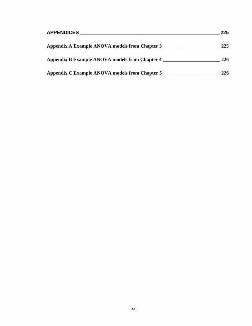
Table 3.25. Planned pairwise contrasts of various neighbouring plant configurations and
broccoli grown in monoculture with all plots included and with the lowest
yielding plots removed (df=1). Significant results are shown in bold type. ..... 53
Table 3.26. Schematic of plots and number of plants per strip with downy mildew infection
(P. destructor). Plots without a superscript letter in common are significantly
different (P=0.05).............................................................................................. 54
Table 3.27. Mean downy mildew (P. destructor) incidence with Plot 5 removed. Plots
without a superscript letter in common are significantly different (P=0.05). ... 55
Table 3.28. Mean downy mildew (P. destructor) incidence compared to neighbouring plant
configurations.................................................................................................... 55
Table 3.29. Planned pairwise contrasts of downy mildew (P. destructor) incidence and
various neighbouring plant configurations and onion monoculture (df=1). ..... 55
Table 3.30. Mean downy mildew (P. destructor) incidence compared to neighbouring plant
configurations with Plot 5 results removed....................................................... 56
Table 3.31. Planned pairwise contrasts of the average downy mildew (P. destructor)
incidence and various neighbouring plant configurations and onion monoculture
with Plot 5 data removed (df=1)........................................................................ 56
Table 3.32. Percentage of the broccoli harvest rejected due to white blister rust (A. candida)
compared to neighbouring plant configurations. Neighbouring plants without a
superscript letter in common are significantly different (P=0.05). ................... 57
Table 3.33. Neighbouring plant row comparisons of the percentage of broccoli heads
rejected at each cut due to infection with white blister rust (A. candida).
Significant results are shown in bold type. Neighbouring plants within columns
without a superscript letter in common are significantly different (P=0.05). ... 58
Table 3.34. Planned pairwise contrasts of the percentage of harvested broccoli heads
rejected due to white blister rust (A. candida) of various neighbouring plant
configurations and broccoli monoculture (df=1)............................................... 58
Table 3.35. Planned pairwise contrasts of the percentage of broccoli heads rejected at each
cut due to white blister rust (A. candida) of various neighbouring plant
configurations and broccoli monoculture (df=1)............................................... 59
xvi
Table 3.36. Mean plot percentages of harvested broccoli heads rejected due to white blister
rust (A. candida) ± SE. Plots without a superscript letter in common are
significantly different (P=0.05)......................................................................... 60
Table 3.37. Mean plot percentages of harvested broccoli heads rejected at each cut due to
infection with white blister rust (A. candida) ± SE. Significant results are shown
in bold type. Plots within columns without a superscript letter in common are
significantly different (P=0.05)......................................................................... 60
Table 3.38. Neighbouring plant configurations and the incidence of diamondback moth (P.
xylostella) larvae per plant. ............................................................................... 61
Table 3.39. Planned pairwise contrasts of the incidence of diamondback moth (P.
xylostella) in neighbouring plant row configurations and the broccoli
monoculture (df=1)............................................................................................ 62
Table 3.40. Plot yield rankings and Fishers LSD groupings of the three crops................... 63
Table 3.41. Rain gauge measurements (mm) from 11/2/04 (#1) and 17/02/04 (#2) from the
locations illustrated on Figure 3.4. .................................................................... 64
Table 4.1. Mean monthly meteorological data for Forthside from September to March in
04/05 and 05/06 with long term averages in brackets....................................... 95
Table 4.2. The effect of treatment (four cropping systems) and planned comparisons of the
abundance of P. xylostella larvae in 04/05. Significant results are shown in bold
type. ................................................................................................................... 97
Table 4.3. Mean number of parasitised P. xylostella per 20 larvae from 04/05. ................. 98
Table 4.4. The effect of treatment (four cropping systems) and planned comparisons of the
parasitism rates of P. xylostella fourth instar larvae collected in 04/05............ 98
Table 4.5. The effect of treatment (four cropping systems) and planned comparisons of the
abundance of P. xylostella pupae in 04/05. Significant results are shown in bold
type. ................................................................................................................... 99
Table 4.6. The effect of treatment (six cropping systems) and planned comparisons of the
abundance of P. xylostella adult moths in 05/06. Significant results are shown
in bold type...................................................................................................... 101
Table 4.7. Average number of eggs oviposited by P. xylostella on leaf samples in the adult
moth laboratory cage ± SE. ............................................................................. 102
xvii
Table 4.8. ANOVA model and planned comparisons of the number of eggs oviposited by
P. xylostella on leaf samples in the adult moth laboratory cage in 05/06. ...... 103
Table 4.9. The effect of treatment (six cropping systems) and planned comparisons of the
abundance of P. xylostella eggs in 05/06. Significant results are shown in bold
type. ................................................................................................................. 104
Table 4.10. Mean number of P. xylostella eggs oviposited on plants in exclusion cages in
05/06. Treatments without a letter in common are significantly different
(P=0.05). ......................................................................................................... 105
Table 4.11. The effect of treatment (six cropping systems) and planned comparisons of the
abundance of P. xylostella eggs oviposited on plants in exclusion cages in
05/06. Significant results are shown in bold type. .......................................... 106
Table 4.12. Comparison of outcomes for P. xylostella eggs oviposited in the exclusion cage
experiment....................................................................................................... 107
Table 4.13. The effect of treatment (six cropping systems) and planned comparisons of the
abundance of P. xylostella larvae in 05/06. Significant results are shown in bold
type. ................................................................................................................. 110
Table 4.14. The effect of treatment (four cropping systems) and planned comparisons of the
abundance of P. rapae larvae in 04/05. Significant results are shown in bold
type. ................................................................................................................. 112
Table 4.15. The effect of treatment (six cropping systems) and planned comparisons of the
abundance of P. rapae eggs in 05/06. Significant results are shown in bold type.
......................................................................................................................... 114
Table 4.16. The effect of treatment (six cropping systems) and planned comparisons of the
abundance of P. rapae larvae in 05/06. Significant results are shown in bold
type. ................................................................................................................. 116
Table 4.17. The effect of treatment (four cropping systems) and planned comparisons of the
proportion of sampled plants with B. brassicae colonies in 04/05. Significant
results are shown in bold type. ........................................................................ 120
Table 4.18. The effect of treatment (four cropping systems) and planned comparisons of the
proportion of sampled plants with parasitised B. brassicae in 04/05. Significant
results are shown in bold type. ........................................................................ 122

xviii
Table 4.19. The effect of treatment (six cropping systems) and planned comparisons of the
abundance of alate B. brassicae in 05/06. Significant results are shown in bold
type. ................................................................................................................. 124
Table 4.20. B. brassicae colonies in 05/06 logistic regression estimates with P values in
brackets. Significant tests are shown in bold type. ......................................... 126
Table 4.21. B. brassicae parasitism in 05/06 logistic regression estimates with P values in
brackets. Significant tests are in bold type...................................................... 128
Table 4.22. The effect of treatment (Cover crop and Bare soil) on the abundance of insects
in the semi-commercial trial at Gawler in 05/06. Significant results are shown
in bold type...................................................................................................... 130
Table 5.1. Potato treatment yields 04/05............................................................................ 143
Table 5.2. The effect of treatment (four cropping systems) and planned comparisons of
potato yield and quality in 04/05..................................................................... 144
Table 5.3. The effect of treatment (four cropping systems) and planned comparisons of
broccoli leaf area and plant biomass in 04/05. Significant results are shown in
bold type.......................................................................................................... 146
Table 5.4. The effect of treatment (four cropping systems) and planned comparisons of the
number of days from transplanting to harvest in 04/05. Significant results are
shown in bold type. ......................................................................................... 147
Table 5.5. The effect of treatment (four cropping systems) and planned comparisons of
harvested head weight per plant in 04/05. Significant results are shown in bold
type. ................................................................................................................. 148
Table 5.6. The effect of treatment (six cropping systems) and planned comparisons of the
number of leaves per plant in 05/06. Significant results are shown in bold type.
......................................................................................................................... 150
Table 5.7. The effect of treatment (six cropping systems) and planned comparisons of total
leaf dry weight in 05/06. Significant results are shown in bold type. ............. 152
Table 5.8. The effect of treatment (six cropping systems) and planned comparisons of mean
leaf dry weight per plant in 05/06. Significant results are shown in bold type.
......................................................................................................................... 154

xix
Table 5.9. The effect of treatment (six cropping systems) and planned comparisons of stem
dry weight in 05/06. Significant results are shown in bold type. .................... 157
Table 5.10. The effect of treatment (six cropping systems) and planned comparisons of the
number of branches per plant in 05/06. Significant results are shown in bold
type. ................................................................................................................. 159
Table 5.11. The effect of treatment (six cropping systems) and planned comparisons of
stem length in 05/06. Significant results are shown in bold type.................... 160
Table 5.12. Proportion of plants with initiated heads at 36 DAT ± SE. ............................ 162
Table 5.13. The effect of treatment (six cropping systems) and planned comparisons of
head diameter development in 05/06. Significant results are shown in bold type.
......................................................................................................................... 163
Table 5.14. The effect of treatment (six cropping systems) and planned comparisons of the
number of days from transplanting to harvest in 05/06. Significant results are
shown in bold type. ......................................................................................... 164
Table 5.15. The effect of treatment (six cropping systems) and planned comparisons of the
harvested head weight per plant in 05/06. Significant results are shown in bold
type. ................................................................................................................. 165
Table 5.16. The effect of treatment (six cropping systems) and planned comparisons of the
branching angle score in 05/06. Significant results are shown in bold type. .. 166
Table 5.17. The effect of treatment (six cropping systems) and planned comparisons of the
shape score in 05/06. Significant results are shown in bold type.................... 167
Table 5.18. The effect of treatment (six cropping systems) and planned comparisons of
hollow stem score in 05/06. Significant results are shown in bold type. ........ 168
Table 5.19. The effect of treatment (six cropping systems) and planned comparisons of on
the potassium content per plant in 05/06. Significant results are shown in bold
type. ................................................................................................................. 169
Table 5.20. Broccoli crop enterprise budget of the Bare Soil Monoculture and the Cover
Crop Monoculture Treatment harvest means and is based on current cash crop
budgets (DPIW 2005). .................................................................................... 177
Table 7.1. Toxicity of insecticides registered for broccoli in Australia (APVMA [2006] and
associated Material Safety Data Sheets) ......................................................... 192
xx
List of Figures Figure 3.1. Experimental design for 03/04. ......................................................................... 28
Figure 3.2. Schematic of naming of a middle 4.95m potato strip cropping strip (left) and a
schematic of a 4.95m potato strip cropping strip on a plot edge (right). .......... 37
Figure 3.3. Schematic of naming of a middle 4.95m onion strip cropping strip (left) and a
schematic of a 4.95m onion strip cropping strip on a plot edge (right). ........... 39
Figure 3.4. Rain gauge locations superimposed onto the experimental design. .................. 64
Figure 4.1. Experimental design 04/05. P=potato, B=broccoli and diagonal lines=cover
crop.................................................................................................................... 81
Figure 4.2. Experimental design 05/06. Where green=potato strips, yellow=rye strips,
grey=cover crop broccoli and clear=bare soil broccoli..................................... 83
Figure 4.3. Sampling schematic for 05/06 experiment, where the numbers indicate a
broccoli plant and the highlighted plants were “selectable”. ............................ 87
Figure 4.4. The mean number of P. xylostella larvae per plant sampled in 04/05 ± SE. “ns”
not significant; * P ≤ 0.05; ** P ≤ 0.01; *** P ≤ 0.001. Points without a letter
in common are significantly different (P=0.05)................................................ 96
Figure 4.5. The mean number of P. xylostella pupae per plant sampled in 04/05 ± SE. “ns”
not significant; ** P ≤ 0.01. Points without a letter in common are significantly
different (P=0.05).............................................................................................. 99
Figure 4.6. P. xylostella vacuum sampling results with female moths from the six
treatments ± SE (left) and the male moths from the six treatments ± SE (right).
Cc-M = Cover crop/Monoculture; Cc-Ry = Cover crop/Rye strips; Cc-Po =
Cover crop/Potato strips; Bs-M = Bare soil/Monoculture; Bs-Ry = Bare soil
/Rye strips; Bs-Po = Bare soil /Potato strips; Male moths captured 36 DAT
(blue columns on the right) without a letter in common are significantly
different (P=0.05)............................................................................................ 101
Figure 4.7. The mean number of P. xylostella eggs per plant sampled in 05/06 ± SE. “ns”
not significant; * P ≤ 0.05; ** P ≤ 0.01; *** P ≤ 0.001. Points without a letter
in common are significantly different (P=0.05). ............................................ 104

xxi
Figure 4.8. The probabilities of the three outcomes from the cage egg survival experiment
where the eggs could have been predated (Attacked), hatched (Hatched) or were
missing (Missing)............................................................................................ 108
Figure 4.9. The mean number of P. xylostella larvae per plant sampled in 05/06 ± SE. “ns”
not significant; * P ≤ 0.05; ** P ≤ 0.01; *** P ≤ 0.001. Points without a letter
in common are significantly different (P=0.05).............................................. 109
Figure 4.10. P. xylostella populations at each 05/06 sample as eggs, 1st, 2nd, 3rd and 4th
instars or pupae. .............................................................................................. 111
Figure 4.11. The mean number of P. rapae larvae per plant sampled in 04/05 ± SE. “ns” not
significant; * P ≤ 0.05. Points without a letter in common are significantly
different (P=0.05)............................................................................................ 112
Figure 4.12. The mean number of P. rapae eggs per plant sampled in 05/06 ± SE. “ns”
indicates that there were no significant differences for that sampling date. ... 114
Figure 4.13. The mean number of P. rapae larvae per plant sampled in 05/06 ± SE. “ns”
not significant; * P ≤ 0.05. Points without a letter in common are significantly
different (P=0.05)............................................................................................ 116
Figure 4.14. P. rapae populations at each 05/06 sampling date summarised as: eggs; 1st and
2nd instar (small) ; 3rd and 4th instars (medium); 5th instar (large); and pupae. 118
Figure 4.15. The percentage of sampled plants in 04/05 with B. brassicae colonies present.
“ns” not significant; ** P ≤ 0.01; *** P ≤ 0.001. Points without a letter in
common are significantly different (P=0.05).................................................. 120
Figure 4.16. The percentage of plants sampled in 04/05 with parasitised B. brassicae. ** P
≤ 0.01; *** P ≤ 0.001. Points without a letter in common are significantly
different (P=0.05)............................................................................................ 122
Figure 4.17. The mean number of alate B. brassicae per plant sampled in 05/06. ** P ≤
0.01; *** P ≤ 0.001. Points without a letter in common are significantly
different (P=0.05)............................................................................................ 124
Figure 4.18. The probability of B. brassicae presence on broccoli plants with 95%
confidence intervals. ....................................................................................... 127
Figure 4.19. Probability of B. brassicae parasitism with 95% confidence intervals. ........ 129
xxii
Figure 4.20. Mean number of various insects and eggs from the semi-commercial trial at
Gawler taken 23 DAT in 05 ± SE. “ns” not significant; * P ≤ 0.05. ............. 130
Figure 5.1. The percentage by weight of the 04/05 potato harvest allocated to each quality
category ± SE .................................................................................................. 144
Figure 5.2. Mean broccoli plant partitioning results from 04/05 ± SE, ns” not significant; *
P ≤ 0.05; ** P ≤ 0.01. Individual columns within each group without a letter in
common are significantly different (P=0.05).................................................. 146
Figure 5.3. The mean number of days from transplanting to harvest in 04/05 ± SE.
Treatments without a letter in common are significantly different (P=0.05). 147
Figure 5.4. Broccoli mean harvested head weights in 04/05 ± SE. ................................... 148
Figure 5.5. Total combined broccoli yields per plot in 04/05. DAT=days after transplanting.
......................................................................................................................... 149
Figure 5.6. Mean number of leaves of broccoli plants in 05/06 ± SE. “ns” not significant;
*** P ≤ 0.001. Points without a letter in common are significantly different
(P=0.05). ......................................................................................................... 150
Figure 5.7. The log of total leaf dry weight per plant from 05/06 ± SE. * P ≤ 0.05; *** P ≤
0.001. Points without a letter in common are significantly different (P=0.05).
......................................................................................................................... 152
Figure 5.8. Mean leaf dry weight in 05/06 ± SE. ** P ≤ 0.01; *** P ≤ 0.001. Points without
a letter in common are significantly different (P=0.05).................................. 154
Figure 5.9. Log of mean stem dry weight 05/06 ± SE. *** P ≤ 0.001. Points without a letter
in common are significantly different (P=0.05).............................................. 156
Figure 5.10. Mean number of branches arising from and including the main stem ± SE. ***
P ≤ 0.001. Treatments in each group without a letter in common are
significantly different (P=0.05)....................................................................... 158
Figure 5.11. Mean stem length of broccoli plants from 05/06 ± SE. “ns” not significant; * P
≤ 0.05; ** P ≤ 0.01; *** P ≤ 0.001. Points without a letter in common are
significantly different (P=0.05)....................................................................... 160
Figure 5.12. Mean head diameter development of broccoli plants in 05/06 ± SE. *** P ≤
0.001. Points without a letter in common are significantly different (P=0.05).
......................................................................................................................... 162
xxiii
Figure 5.13. The mean number of days from transplanting to harvest in 05/06 ± SE.
Treatments without a letter in common are significantly different (P=0.05). 164
Figure 5.14. Broccoli mean harvested head weights in 05/06 ± SE. Treatments without a
letter in common are significantly different (P=0.05). ................................... 165
Figure 5.15. Mean branching angle score (1-5) in 05/06 ± SE, where 1=worst branching
angle (unmarketable) and 5=best branching angle (highly marketable). ........ 166
Figure 5.16. Mean shape score (1-5) in 05/06 ± SE, where 1=worst shape (unmarketable)
and 5=best shape (highly marketable)............................................................. 167
Figure 5.17. Mean hollow stem score (1-4) in 05/06 ± SE, where 1=severe hollow stem and
4=no hollow stem. ........................................................................................... 168
Figure 5.18. Mean Potassium (K) content of nutrient sap tests in 05/06 ± SE. Treatments
without a letter in common are significantly different (P=0.05). ................... 169

xxiv
List of Pictures Picture 3.1. Onions planted into three beds per strip with 8 rows of onions per bed........... 30
Picture 3.2. Onions after lifting............................................................................................ 30
Picture 3.3. Onion yield sampling using a 0.5m2 quadrat.................................................... 31
Picture 3.4. Onions bagged for yield sampling, Plot 4 (left) and Plot 1 Onion monoculture
(right)................................................................................................................. 31
Picture 3.5. Onion size scale (left to right) >70mm, 60-70mm, 50-60mm, 40-50mm and
<40mm. ............................................................................................................. 31
Picture 3.6. Onion grading equipment. ................................................................................ 32
Picture 3.7. Onion harvester (left) and close up of the harvester’s lifter (right). ................. 32
Picture 3.8. Front view (left) and rear view (right) of the potato planter............................. 33
Picture 3.9. Technical Officer assuring potato set regularity............................................... 33
Picture 3.10. Potato yield sample being marked (left) and dug with a potato fork (right). . 33
Picture 3.11. Technical officer taking potato yield samples. ............................................... 34
Picture 3.12. Six row broccoli transplanter, rear view (left) front view (right). .................. 34
Picture 3.13. The push weeder. ............................................................................................ 35
Picture 3.14. (a). Manual harvesting (cutting) of broccoli (left). (b). Harvesting broccoli
into bags hung by nails on the inside of two half tonne bins (right). ................ 36
Picture 3.15. Scale of infection of harvested broccoli heads with white blister rust (Albugo
candida) progressing from a no infection (left) to a high infection (right) likely
to lead to rejection at the factory....................................................................... 36
Picture 3.16. Downy mildew (P. destructor) symptoms...................................................... 54
Picture 3.17. (a). Yellowing of onions visible after the removal of neighbouring broccoli
plants (left). (b). A broccoli leaf partially shading an onion plant (right)......... 66
Picture 3.18. Complementarity of potato and broccoli leaf canopies on a strip edge with
potatoes on the left and broccoli on the right. .................................................. 67
Picture 4.1. A P. xylostella adult moth (left), pupa and 4th instar (middle) and three different
instars (right), the middle and right pictures also illustrate “windowing” of the
leaves due to larval feeding............................................................................... 73
Picture 4.2. A P. rapae adult (left) and P. rapae larvae (middle) P. rapae chrysalid. ........ 74
xxv
Picture 4.3. An alate B. brassicae adult with nymphs (left), an aphid colony with a
Diaeretiella rapae wasp (middle), and an aphid colony with parasitised (brown)
mummies (right)................................................................................................ 75
Picture 4.4. Treatments for the 04/05 experiment (clockwise from top left) Cover
crop/Monoculture . Cover crop/Potato strips, Bare soil/Monoculture, Bare
Soil/Potato strips. .............................................................................................. 82
Picture 4.5. Additional treatments for the 05/06 experiment: Bare soil/Rye strips (left)
Cover crop/Rye strips (right). Note that the photos were not taken on the same
day. .................................................................................................................... 83
Picture 4.6. The author inspecting broccoli plants using jewellers glasses. ........................ 87
Picture 4.7. (a). Exclusion cage with netting before placement (left). (b). An uncovered
cage surrounding a broccoli plant (right). ......................................................... 90
Picture 4.8. Placing moths in exclusion cages, with the moth containers and equipment
(left) and re-sealing the entrance hole (right).................................................... 90
Picture 4.9. P. rapae pupating on an onion plant............................................................... 119
Picture 5.1. Potato Cover crop/Monoculture after planting 04/05. .................................... 140
Picture 5.2. Digging (left) and bagging (right) potatoes from the 04/05 experiment. ....... 140
Picture 5.3. A plant marked for harvest with a white stick. ............................................... 142
Picture 5.4. Head shape – convex (5) to concave (1) (left) and branching angle tight (5) to
spreading (1) (right) scales from (Tan et al. 1999). ........................................ 142
Picture 5.5. Broccoli hollow stem scale with rankings in brackets (from left) – no hollow
stem (4), trace (3), minor (2) and severe (1). .................................................. 143
Picture 5.6. An unweeded area between two plots in 05/06 experiment ........................... 172
Picture 5.7. Infestation of wild radish in the 04/05 experiment controlled by the rye cover
crop on the right, with the interplot region marked with a black line. Note that
the plot pictured in Picture 5.8 is in the background....................................... 173
Picture 5.8. Infestation of wild radish in a bare soil plot in the 04/05 experiment, with the
interplot area marked with a black line. .......................................................... 174
Picture 5.9. Control of wild radish by the unweeded cover crop at 48 DAP in the 04/05
experiment....................................................................................................... 174
Picture 6.1. (a). Side view of a Turbo Teejet® (left). (b). Assembling the sprayer (right).179
xxvi
Picture 6.2. (a). Sprayer end guard in profile with pop rivets indicated by the arrow (left).
(b). The end guard attachment (right). ............................................................ 180
Picture 6.3. The end guard between two crops. ................................................................. 180
Picture 6.4. (a). Sprayer rear view (left). (b). The sprayer front view (right). ................... 181
Picture 6.5. Cover crop in the 04/05 experiment prior to desiccation and rolling. ............ 182
Picture 6.6. (a). The heavy roller with two trailing discs (left). (b). A demonstration of the
angle iron flattener (right). .............................................................................. 182
Picture 6.7. (a). Pre-drilling fertiliser into a flattened cover crop (left). (b). Hand planting
broccoli plants (right). ..................................................................................... 183
Picture 6.8. (a). Roller construction with the drum and angle iron “crimpers” indicated by
the arrow (left). (b). Attaching the roller to the tractor tool bar (right)........... 184
Picture 6.9. (a). The roller with the fertiliser box attached indicated by the arrow (left). (b).
A cup planter unit indicated by the arrow (right)............................................ 184
Picture 6.10. (a). The double disc openers (indicated by the arrow) attached to the cup
planter (left). (b). The trash guard (indicated by the arrow) attached to the
double disc unit (right). ................................................................................... 185
Picture 6.11. The prototype roller/transplanter ready for testing ....................................... 186
Picture 6.12. The prototype roller/transplanter being tested in the semi-commercial trial in
05/06................................................................................................................ 186
Picture 6.13. (a). The second prototype roller with slot maker (left). (b). A close up of the
slot makers (right). .......................................................................................... 187
Picture 6.14. (a). The second prototype ready for testing (left). (b). The fertiliser box drive
system attached to the roller (indicated by the arrow) (right). ........................ 187
Picture 6.15. The end result of the second prototype roller/transplanter, a rolled cover crop
and transplanted broccoli (Cover crop/Rye strips Treatment). ....................... 188
xxvii
Glossary of Terms Strip crops – growing two or more crops in tractor width repetitions.
Cover crops – plants grown for ground cover that are killed prior to planting a commercial
crop.
Bare soil – soil without ground cover that has been cultivated to a fine tilth.
Oviposition – the process of an insect depositing an egg.
DAT – number of days after a seedling has been transplanted.
Host location – the process an insect undertakes when attempting to find a suitable host
plant.
Cosmopolitan insect – an insect that is found wherever its host plant is cultivated.
Instar – a post embryonic insect growth stage between moults.
Alatae – winged female aphids.
Apteratae – wingless female aphids.
Degenerate – having lost highly developed functions, characteristics or structures through
evolution.
Gravid – carrying developing young or eggs.

xxviii
Acknowledgements This research was made possible by a number of individuals and an Australian
Postgraduate Award scholarship from the University of Tasmania. Further provision of
financial support in the form of a scholarship “top-up” and operating funds from Professor
Rob Clark and TIAR is gratefully acknowledged. It is very unusual for a postgraduate
student to be given as much latitude to research a topic of his or her own choosing, and I
am truly thankful for the opportunity I was afforded.
I would like to acknowledge the in-kind contributions of the Tasmanian Department of
Primary Industries and Water, Harvest Moon, Simplot and Field Fresh. Thanks go to Peter
Aird from Serve-Ag for his advice on chemical treatments and his general support for my
overarching research goals. Thanks are due to the staff at Forthside Research and
Development Station.
My supervisors Dr. Shaun Lisson and Dr. Neville Mendham deserve thanks as they
provided valuable guidance for this project and significant editorial effort. Dr. Nancy
Schellhorn was an invaluable resource in helping design and analyse my final years trials. I
thank Dr. David Ratkowski and Dr. Ross Corkrey for statistical advice and Dr. Nancy
Endersby for kick starting my laboratory Plutella population.
A special commendation must go to my father Ian Broad for his significant contribution to
this thesis in the way of advice, acting as a sounding board, assistance in harvesting
broccoli, the provision of land for my semi-commercial trail and finally allowing me free
reign of his shed, equipment and junk pile for the building of the roller/transplanter.
Without his help I doubt this thesis would have happened.
Last, but not least, I would like to thank my partner Alicia for her help establishing trials
and for being willing to move with me to Forth, making the long hours of trial work
possible (and bearable).

1
Chapter 1 Introduction This thesis began as a personal concern rather than an immediate industry based problem.
This concern started to develop as I grew up on my parent’s mixed crop and livestock
property, on the northwest coast of Tasmania, and continued to develop as I worked as a
contract vegetable grower before attending University and completing my degree in
Agricultural Science. During these years, vegetable production systems increased in scale,
and in the process become more reliant on agrochemicals to control competing organisms.
My developing apprehension was that agriculture was becoming too reliant on chemicals
inputs, which had the potential to increase problems in the future and was perhaps not the
best way forward for the industry. These points initiated the question, “Are there any
feasible alternatives?” This question forms the starting point of this thesis. However, before
beginning to explore this question, the reasons for the current trends in vegetable
production systems need to be understood.
1.1 Current trends in modern vegetable production systems
Since the geographical expansion of agriculture slowed markedly in the 1950’s, crop yield
increases accelerated, more than keeping pace with population growth. This resulted in a
worldwide oversupply of food (Swaminathan 2004). Globalisation in agriculture and the
continued breakdown of trade barriers enlarged the market available to Australian farmers
but also increased the number of competitors (Barr 2004). Both oversupply and
globalisation have meant continued downward pressure on agricultural product prices and
declining margins between real farm receipts and real farm costs (Laurence 2000). This
has led to worldwide structural changes in agriculture over the last four decades
characterised by increased mechanisation, intensification of production, increasing use of
external inputs and the separation of livestock and crop production (Knickel 1990).
On average, over the last 15 years, agricultural output in the Organisation for Economic
Co-operation and Development (OECD) countries has increased by 15%, on 1% less land
with 8% fewer workers. At the same time the inflation adjusted price of food has fallen by
approximately 1% per annum (Legg and Viatte 2001). To remain globally competitive
2
Australian farms have become larger, more capital intensive and fewer in number (Garnaut
and Lim-Applegate 1998). There has also been increasing pressure to specialise rather than
diversify (Stuthman 2002) as specialisation brings economies of scale though greater
mechanisation, the use of hybrid germplasm and the focusing of knowledge, research and
marketing (Vandermeer et al. 1998). Only 50 years ago vegetable producers in Australia
were small, diverse, labour intensive operations on the urban fringe with few chemicals and
fertilisers available. In comparison, modern vegetable producers are highly productive,
large scale, increasingly specialised operations dependent on irrigation, fertiliser,
agrochemicals, transport and marketing systems and found in regions where the climate,
soil and water supplies are most suited to the production of specific crops (Stirzaker 1999).
Access to markets and the relative prices of outputs and inputs strongly influence the
selection of crop types, crop sequences and crop management (Boiffin et al. 2001).
While these farming systems are extremely productive and provide low-cost food (Altieri
1998; Stirzaker 1999) they also bring a variety of economic, environmental and social
problems (Altieri 1998). A focus on maximising production in the short-term without
consideration of the consequences on other essential components of the agro-ecosystem has
led to natural resource degradation in Australia (Williams and Gascoigne 2003). The
annual cost of this resource degradation, which includes salinity, acid soils, soil structural
decline, erosion, irrigation salinity, reduced water quality and invasive weed control, has
been estimated to be in excess of $A 3.5 billion (Standing Committee on Environment
Recreation and Arts 2001).
At the individual farm level there has also been a subsumption of the decision making
process by corporations as part of the contracting process (Tonts and Black 2002). For
example, in Tasmania, vegetable processing companies make most of the decisions in
relation to the selection of varieties, planting and harvesting dates, irrigation schedules,
chemical applications and fertiliser requirements, and usually award annual contracts less
than a year in advance (Miller 1995). This compounds the imbalance between economic
and environmental imperatives, as there is little opportunity for forward planning and
attempts to achieve sustainability are afforded low priority (Miller 1995).
3
There are very few native Australian plants that are grown as crops in any capacity. Instead
crops are drawn from a diverse range of geographic locations, from South America to
Europe. As a result the remnant ecosystems dispersed throughout the cropping locations
have a long evolutionary history distinct from that of the introduced crops (Hill 1993).
Therefore most pests, predators and diseases are also exotic in their origin. The insect pest
situation is further complicated as many species have the ability to migrate in large
numbers on favourable winds, at times inundating biological control mechanisms (Hill
1993).
These factors, combined with modern agriculture’s reduced tolerance of weeds, pests and
diseases (Vandermeer et al. 1998), means maintaining the productivity of soils and
sustaining the rural environment in the face of declining farm profitability, is seen as the
single most important issue in many agricultural industries today (Laurence 2000).
Furthermore, Trewavas (1999) suggests that along with abundant (and cheap) food and
greater life expectancies, has come a demand from consumers for a risk free world. Since
modern farming practices have been fairly or unfairly associated with chemicals and health
risks, there is an increasing demand for ‘clean green’ chemical free food. There have also
been calls for greater use of ‘sustainable’ production methods in Australia due to continual
scrutiny of agricultural production methods by an increasingly urbanised population
coupled with an agricultural lobby with waning political power (Barr 2004). These
demands are increasingly being reflected in the requirements of retailers, particularly the
economically powerful supermarkets in Europe (Gunningham and Sinclair 2002) and
Australia.
In summary, the current trends in Australian vegetable production are that increased global
supply and competition has resulted in increased farm efficiency, management simplicity,
greater reliance on inputs (including agrochemicals) and increased scrutiny by a largely
urban public who desire “sustainably” produced goods. Therefore, research into vegetable
cropping systems that maintain efficiency and productivity, but at the same time reduce the
level of chemical inputs, could result in more marketable products and be an alternative to a
4
continued reliance on chemical solutions. Researching strategies to reduce chemical
dependence in vegetable production also aligns well with current Australian agricultural
policy statements, for example Tasmania’s state government policy and promotion of
Tasmanian agricultural industries as being “clean and green”, with low chemical usage, and
a moratorium on any use of gene technology in the production of food (Anon 2003b).
1.2 Steps in this research
The search for a feasible alternative to the current trend of increased chemical dependence
in vegetable production systems, initially involved discussing the problems of chemical
dependence and the benefits and disadvantages of farming systems with reduced chemicals
requirements. This led to the initial choice of research direction that was further developed
via a review of relevant literature (Chapter 2). This in turn generated specific research
questions, with preliminary field investigations commencing in the summer of 2003/2004
with the strip cropping of potatoes (Solanum tuberosum), broccoli (Brassica oleracea var.
italica) and onions (Allium cepa) (Chapter 3). Initially this project was conceived as a
broad look at problems and potential solutions to chemical dependence in each of these
three vegetable crops. However, the results from the initial trial demonstrated that the most
interesting trends were occurring in broccoli, which is a good example of an intensively
produced vegetable with the associated problems of insect pest pressure, insecticide
resistance, weed pressure and rapid growth. Therefore the majority of the work in the
following two years concentrated on broccoli as a key part of an intensive system. The
major focus of this thesis relates to the impact of cover and strip cropping on insect
populations in broccoli (Chapter 4). Agronomic and economic impacts are discussed in
Chapter 5 and machinery design aspects in Chapter 6. The research detailed in this thesis
covers a wide range of subject matter within the field of agricultural science including
agronomy, entomology and agricultural engineering. The final chapter, Chapter 7,
summarises these different aspects and discusses future research directions.
5
Chapter 2 Literature review
2.1 The problems of chemical dependence in agricultural
production systems
“[T]oo often current agricultural production in the industrialized world can be
characterized as too many people trying to grow the same crop (perhaps even the
same or very similar varieties of that crop) in much the same manner.” (Stuthman
2002)
The initial success of DDT (dichlorodiphenyl-trichlorethane) in the 1930s shifted scientists
away from fundamental research on insect biology, physiology and alternate methods of
pest control, to developing synthetic organic insecticides for the control of pests. The rapid
expansion of insecticide research also resulted in the development of chemicals to control
pathogens and weeds. Along with yield gains from the Green Revolution came the
economic incentive to chemically protect these yields from pests, pathogens and weed
competition (Ruttan 1999).
The economic benefits of chemical protectants, coupled with the economic pressures
detailed in the Introduction, has resulted in modern agriculture being characterised by
large-scale deployment of genetically uniform seed, tubers or plantlets. This practice has
led to both management and genetic simplicity and uniformity on modern farms, and
indeed across regions and even countries. Herein lies the foundations of a disease epidemic
because if one plant is susceptible to a disease, then vast areas can potentially allow almost
limitless expansion of a pathogen (Wolfe 2000). The worst incidences of breakdowns in
resistance leading to plant disease epidemics are the 1840’s potato famine in Ireland caused
by Phytophtora infestans, the Bengal rice famine of 1942-1944 caused by
Helminthopsporium oryzae, and the 1970’s Southern Corn Blight epidemic caused by
Fusarium graminearum (Stuthman 2002). To halt these problems, scientists have
developed new chemicals or resistant varieties (Wolfe 2000). However, these practices

6
place greater selection pressure on pathogens to adapt (Ruttan 1999; Mundt et al. 2002)
resulting in what is effectively an arms race between scientists and pathogens.
Similar trends are evident in the control of insects as the development of DDT led to a pest
control strategy based on total annihilation (Vandermeer 1995) and frequent pesticide
applications. This strategy in some instances resulted in resistance, the loss of beneficial
insects and increased pest damage. Increasing the number of applications could sustain
yields in the short-term but productivity could still collapse (Conway 1987). An example
was the cotton industry in the Ord Valley of Western Australia where resistance of
Helicoverpa armigera to DDT resulted in up to 35 applications of insecticides per season
and eventual failure of the industry (Fitt 1994). This situation is not unique to one industry
as multiple chemical resistance has also been detected in many other insect species and is
increasing despite the introduction of new classes of insecticide (Denholm et al. 2002).
The practice of “clean” cultivation means that producers also attempt to eliminate crop
competition from weeds and often herbicides are the simplest, most reliable and cheapest
method of weed control available (Heap 1997). As a result, growers spend more money on
herbicides than any other crop input (Marshall et al. 2003). Once again the reliance on
chemical management has resulted in resistance problems. Resistant weed species include
at least 40 dicotyledonous plants and 17 monocotyledonous plants (Holt et al. 1993). While
resistance to triazine herbicides are most commonly reported (Holt et al. 1993; Heap 1997),
at least 60 weed species have biotypes resistant to one or more herbicides from 14 other
herbicide classes (Holt et al. 1993) and the number of new cases of herbicide resistance has
a relatively constant average of nine per year (Heap 1997).
As well as the resistance of insects, pathogens and weeds to chemical controls the
increasing reliance on chemicals in modern agricultural production can have other side
effects, both real and perceived. Frequent applications of pesticides severely reduce
biological diversity destroying a wide array of susceptible species, changing the normal
structure and function of the ecosystem (Pimentel et al. 1992). Brummer (1998) sums up
the current situation:

7
“Despite millions of dollars of public and private research investment, 50 years of
chemical control have only made weeds and pests more difficult to control; though
chemicals make management simpler in the short run, they invariably create more
extreme problems in the future.”
2.2 Possible options for reducing chemical dependence in
vegetable production systems
Despite the problems of chemical use illustrated above, the widespread use of chemicals, as
part of modern agricultural systems, has bought some distinct benefits including cheap and
abundant food. Simply reducing the use of chemicals in agriculture without implementing
alternatives could be disastrous, amongst other things, potentially exacerbating
vulnerability to crop failure (Clunies-Ross 1995). Some alternatives that could allow a
reduction in chemical use have been suggested and these include: (i) the use of transgenic
crops, or genetically modified organisms (GMOs); (ii) integrated pest management (IPM);
(iii) conversion to “organic” practices; or (iv) applying ecological principles to agricultural
systems.
2.2.1 Transgenic crops
In agricultural systems GMOs can be divided into three classes: (i) those producing an
insecticidal compound isolated from the bacterium Bacillus thuringiensis (Bt); (ii) plants
resistant to some form of broad-spectrum herbicide and; (iii) plants with combinations of
both.
Bt toxins, when ingested by susceptible insects, are activated by the midgut proteases,
which interact with the larval midgut epithelium causing disruption of the membrane
integrity and eventual death (Gill et al. 1992). In genetically modified Bt plants the Bt
genes are inserted into and expressed by the plant. In effect this technology internalises the
application of the insecticidal compounds. To prevent the pervasive ability of some insects
to develop resistance, a refuge strategy has been widely adopted. This entails planting
refuges of non-Bt host plants along with Bt crops to promote survival of susceptible pests.
As resistance alleles are often rare and recessive, the susceptible pests will in effect dilute

8
any resistance that develops, but this in itself does not preclude resistance developing
(Tabashnik et al. 2003). Since cotton containing a single Bt gene was introduced into
Australia to control Helicoverpa sp. in 1996, average reductions in pesticide use of over
50% have been reported (Skerritt 2004). Compare this to the previously mentioned use of
up to 35 sprays per season before the collapse of the cotton industry in the Ord River region
of Western Australia (Fitt 1994).
The use of herbicide resistant plants, whether genetically modified or not, make weed
control much simpler but have the potential to facilitate the development of herbicide
resistant weeds through genetic transfer to closely related weed species and by creating
intense selection pressure for weeds to adapt to the herbicides used. A further problem is
seed dormancy, where the herbicide resistant crop germinates as a volunteer weed the
following year in the next crop grown in rotation. These concerns and others, along with
debate about whether or not herbicide resistant GMOs have improved yields and financial
returns to farmers, have led some weed scientists to question whether these GMOs are
beneficial (for example Martinez-Ghersa et al. [2003]).
There has also been controversy surrounding the development and deployment of
genetically modified organisms in agricultural systems in the public arena. For example,
widely publicised campaigns by environmental groups like Greenpeace, have called on
governments to apply the “precautionary principle” to GMOs where they are banned until
the proponent can conclusively prove that the product is safe for the environment and
human health (van den Belt 2003). This has led to moratoria on the research and use of
GMOs being put in place in some regions, including Tasmania. The Tasmanian State
Government’s rationale behind the moratorium on commercial release of agricultural
(GMOs) until 2008, was to underpin Tasmania’s reputation for ‘clean, green and quality’
products (Anon 2003a) indicating that from a policy perspective the use of GMOs can also
be unpopular.
In spite of the public debate, the use of genetically modified crops can reduce the amount of
chemicals directly applied to crops in some agricultural production systems. However,
9
GMOs do not eliminate chemicals, instead the herbicide use is simplified and/or
insecticides are internalised and expressed by the plant instead of being applied to the plant.
Therefore GMOs can also be seen as a repackaging of chemical technology not a solution
to the dependence on agrochemicals. Furthermore, from a practical viewpoint, GMOs
cannot be researched for this thesis due to the aforementioned moratorium.
2.2.2 Integrated Pest Management
The concept of integrated pest management (IPM) is becoming more popular with farmers,
researchers and policy makers (Thomas 1999) due to concerns over pesticide resistance,
human health and environmental impacts (Mo and Baker 2004). IPM seeks to minimise
reliance on pesticides by emphasising the use of alternative control methods, including
biological control, host plant resistance breeding, cultural techniques (Thomas 1999), and
the development of threshold based spray programs in conjunction with time efficient
sampling techniques (Mo and Baker 2004). The practice of IPM has received by far the
most attention in the quest for “alternative” pest management strategies (Lewis et al. 1997).
IPM is complicated and “knowledge intensive” due to the complexity of interactions
between plants, pests and natural enemies, which make it difficult to apply pest control
prescriptions across all systems (Thomas 1999). This is perhaps why IPM has been adopted
in relatively few crops and has yet to significantly reduce the use of pesticides worldwide
(Matson et al. 1997). In practice IPM has become a monitoring strategy with the
establishment of thresholds, and chemicals used on an as needed basis (Lewis et al. 1997).
Furthermore, corporate planners have embraced IPM because the practice does not
eliminate the need for chemicals but rather requires the development of expensive pest-
specific or environmentally benign chemicals (Rosset and Altieri 1997). Therefore even
with large-scale adoption of IPM, chemical dependence will remain.
2.2.3 Organic production methods
The organic agriculture movement emerged in the 1930’s and 1940’s as an alternative to an
increasingly industrialised agriculture based on nitrogen derived from the Haber-Bosch
process (Lotter 2003). That initial movement has developed into a system that attempts to
10
address concerns some farmers, researchers and consumers have with modern petro-
chemical based farming methods (Kondinin-Group 2000).
A working definition of organic agriculture is “good farming practice without using
synthetic chemicals” (ATTRA 1995). “Organic” typically denotes an agricultural product
grown using practices certified by a recognised organic certification body. In general,
proponents of organic production methods claim the practice is better for the environment
and human health when compared to conventional practices. Organic producers and
consumers also describe organic production methods as being more “natural” and therefore
better than “artificial” conventional practices (Verhoog et al. 2003). It is essential that these
claims are legitimate if organic products are to fulfil the promise that consumers can
substantially change agricultural practice for the betterment of the environment (Allen and
Kovach 2000). To this end, Treadwell et al. (2003) asserts that the ecological and
biological mechanisms behind long held and “often ridiculed” beliefs of organic farmers
are being elucidated. However, others suggest that the claims of the organic movement are
based on “very little science” (Trewavas 2001a) or flawed methodology (for example,
claims that organic products are tastier or more nutritious, as discussed by Lotter [2003]).
Other concerns expressed in relation to organic agriculture include:
• The prevalence of input substitution in organic agriculture where organically
registered, “natural” products are used instead of an industrially produced
pesticides, fungicides or fertilisers, meaning that the system is essentially the same
as conventional production (Rosset and Altieri 1997).
• The consequences of wide scale conversion to organic agricultural production on
the environment. Compared to conventional production, it is widely reported that
across systems organic production methods typically reduce yields by 5% to 60%.
Intensive organic systems have the greatest yield reductions when compared to their
conventional counterparts, while extensive organic systems have marginally
reduced yields compared to conventional systems (Lotter 2003). The outcome of
this yield reduction is that if the world were to feed itself using organic farming
11
principles more agricultural land would be required to produce the same amount of
food as conventional production systems, which could lead to the destruction of
wilderness areas (Legg and Viatte 2001; Trewavas 2001b).
• The reliance on nutrients from conventional farming systems. Organic farms,
especially horticultural operations, rely on wastes from conventional systems in the
form of manures, green waste, household wastes and food industry wastes to
maintain fertility (Guthman 2000; Watson et al. 2002). These nutrient subsidies
from conventional agriculture mean that organic agriculture remain indirectly
dependent on artificial fertilisers and chemicals. Moreover, if there was wide scale
conversion to organic agriculture there might not be adequate supplies of these
wastes for all organic producers.
At present organic production remains a set of rules based on a philosophical standpoint
and not a proven science in its own right. There is also tension within the organic
movement between philosophically committed producers and producers merely operating
within the regulations with ideologies more in common with conventional producers
(Guthman 2000; Treadwell et al. 2003).
In summary, organic systems still use chemicals, albeit chemicals derived from natural
sources. These chemicals can still have serious side effects and environmental impacts
(Altieri and Rosset 1996). Furthermore, in some instances these more “natural” chemicals
can be more toxic than conventional chemicals (for instance “natural” copper sulphate
fungicide compared to the conventional equivalent Mancozeb®, as discussed by Trewavas
[2004]). In a report of organic farming in Australia by the Kondinin-Group (2000) the
majority of concerns about conventional production relate to the use of agrochemicals and
their cost. If reduced chemical usage were the dominant reason for consumers to choose
organic produce, would it be better to develop “conventional” systems that use fewer
chemicals?
12
2.2.4 Farming systems compatible with ecological principles
Ecological principles suggest that current modern agricultural production systems are
relatively unstable and will continue to be prone to invasion by weeds, and high incidences
of pests and diseases (Vaughan 1998; Tilman 1999) and thus require constant external
inputs to perform (Altieri and Rosset 1996). Many of the major pest problems of today are
a direct result of actions taken to improve crop production (Thomas 1999). As a
consequence, commentators have been calling for a shift in research effort to blend ecology
and agricultural science in order to design stable farming systems based on mimicking
species diverse natural systems (Clunies-Ross 1995; Lewis et al. 1997; Matson et al. 1997;
Brummer 1998; Dawson and Fry 1998; Jackson 2002; Rämert 2002).
The recognition that ecological principles can be used in farming is widely accepted as the
calls for more research suggest. However, there are both real and perceived problems in
applying ecological principles to agricultural production systems. The first is which
principles should be used (Wood 1998). Another problem is that the reductionist approach
common in science means that simplified systems are easier to study. As Vandermeer et al.
(1998) states,
“..it is possible that a bias is introduced by agricultural research which has an
adequate tool-box of experiments and models for technology development in
monocultures, but which is less able to deal with more complex systems.”
Furthermore, most soil science and agronomy departments in universities have been
“married to agriculture” and have had only fleeting associations with ecology, ecosystem
studies or earth sciences (Williams and Gascoigne 2003). Together with the current
research paradigm, social pressures, limited funding options, pressure from processors and
financial institutions make it increasingly difficult to change from what is perceived as
“current practice”. As a result there has been little effort to apply ecological theory, models
and techniques to agricultural systems (Robertson 2000).
One possible starting point for the application of ecological principles in agricultural
systems is the ecological theory of diversity/stability, in which species diverse systems are
stable systems that have the ability to resist pest and disease incursions (McCann 2000). An

13
ecological analysis of modern agricultural systems, as discussed in the Introduction, reveals
that genetically homogenous crops do not possess this ecological mechanism to lessen the
impact of pests (Altieri and Rosset 1996). If pest and disease outbreaks that require
chemical interventions are understood as being the result of an ecological imbalance, then
the treatment should be to recover balance or “homeostasis”, which is the maintenance of
the system’s internal functions and defences to compensate for external stresses. The
primary technique for achieving homeostasis, self regulation and sustainability is
biodiversification (Altieri and Rosset 1996), which in the case of vegetable cropping
systems would involve plant species diversification.
The most useful biological standard equivalent of modern vegetable production systems is a
rainforest with sustained high levels of primary production, in wet leaching environments
through efficient cycling of nutrients and water and stress minimisation through species
diversity (Stirzaker 1999). If it is possible to use the rainforest as a biological standard then
it is also possible that some lessons can be learned from nature. In particular, the species
diversity of rainforest systems hinders the development of pest and disease outbreaks. If the
idea of diversity/stability could be successfully introduced into vegetable cropping systems,
there is the potential to reduce pest and disease pressure and therefore reduce the need for
chemical interventions.
2.3 Research options – the best way forward?
Limiting factors in agriculture represent the symptoms rather than the underlying “disease”
inherent in imbalances within the agricultural ecosystem (Altieri and Rosset 1996),
therefore a new production paradigm is required. To discover new production paradigms
the search has to be very broad (Weiner 2003). Any changes are not necessarily
straightforward, as eliminating soluble man-made fertilisers and chemicals completely
would reduce vegetable yields, in turn making vegetables more expensive, reducing
peoples’ intake and increasing cancer rates (Ames and Gold 1997). The movement towards
sustainable agriculture is not simple as Legg and Viatte (2001) have discussed:
“OECD countries know that agriculture needs to be made more sustainable. But it
is not so clear how this can be achieved.”

14
Applying technological solutions like GMOs or large scale conversion to organic
agriculture with its propensity for input substitution, do not address the underlying
ecological causes of environmental problems in agriculture, which are rooted in the
monoculture structure prevalent in large scale production systems (Altieri and Rosset
1996). IPM aims to change conventional practice and reduce chemical use through
monitoring and targeted chemical applications, but is this the best solution to reducing the
use of chemicals in agriculture? This practice does not reduce yields if properly
implemented and can save costs because chemical interventions are only used when
necessary and not on a calendar basis. However, as discussed in Section 2.2.2, IPM in
practice has become little more than a monitoring strategy and the use of more expensive
selective insecticides.
Using ecological principles shows great promise in reducing chemical use in vegetable
cropping systems because experiments have been aimed at treating the underlying causes
rather than treating the symptoms with chemicals (like GMOs and IPM), while also being
more productive than organic systems. However, as discussed, there are some issues in the
use of ecological principles, the most pressing is which ecological principles to use (Wood
1998)? Furthermore, there is a lack of adequate research relating to the integration of
ecological principles with farming system design and no clear guidelines to work from.
With this in mind, the focus of the research in this thesis is on the introduction of greater
diversity/stability in vegetable production systems. The selection of this topic does not
detract from the need for, or benefits of the other approaches such as GMOs, IPM and
organic principles. Indeed, these alternatives for reducing the use of chemicals in vegetable
cropping systems can be incorporated into a species diverse system in the future, potentially
further reducing the use of chemicals.
2.4 Introducing plant species diversity into modern cropping
systems
Consideration should also be given to problems of farmers discussed in the Introduction, as
consumer demands for sustainably produced products go hand in hand with economic
15
demands for low cost production. Farmers are also business people and their primary goal
is to produce food at a profit. Ensuring resource sustainability is not usually their main
objective, therefore the integration of ecological theories needs to be focused on enhancing
ecological and economic benefits (Robertson 2000). This acts as a further barrier as any
change to current cropping systems has to be economically sustainable to be attractive to
farmers. As the adage goes, “It’s hard to be green when you’re in the red.” Therefore,
research should focus on designing simple cropping systems based on the ecology of
simple and productive natural systems (Wood 1998) and not attempting to initially reinvent
the wheel. There are examples of simple species-diverse cropping systems in the
international literature based on an holistic approach to experimentation. These are building
a scientific case for the adoption of diversity in agricultural systems and are typically based
on three main options, which include:
• Side by side diversity - planting strips or rows of different crops together
(intercropping/strip cropping).
• Vertical diversity - growing a taller crop above an understorey plant
(undersowing/cover cropping/living mulches).
• Within crop diversity - planting genetically diverse cultivar mixes (multi-
line/species mixtures).
2.4.1 Side by side diversity – intercropping and strip cropping
Intercropping has been defined as the cultivation of two or more crops in such a way that
they interact agronomically (Vandermeer 1989). Strip cropping is similar except that the
crops are grown in strips wide enough to facilitate separate mechanical management.
Data extracted from 54 experiments by Jolliffe (1997) indicated that, on average, mixtures
of different crops were 12% more productive than pure stands. This could be the result of
temporal production advantages, which can be achieved when different crops with
staggered planting and maturity dates have different resource demands at different times,
lessening or limiting competition between crops (Sullivan 2001; Santos et al. 2002).
Alternating rows of crops can also create edge effects, including greater light interception
and wind sheltering, which can lead to higher production levels than individually planted
16
crops (Clark and Myers 1994; Ayisi et al. 1997; Ghaffarzadeh et al. 1997; Smith and Carter
1998; Lesoing and Francis 1999). Edge effects can also create greater system resilience and
financial risk reduction due to compensatory growth when extra resources (light and
nutrients) are available to one crop if another crop performs poorly (Theunissen 1997;
Wolfe 2002). Companion effects have also been reported, where the interaction of the
different crops can provide cultural benefits like increased nitrogen availability and weed
suppression (Hauggaard-Nielsen et al. 2001). There is also some evidence that
intercropping can reduce insect pest pressure in Brassicas (Bach and Tabashnik 1990;
Meena and Lal 2002).
Intercropping and strip cropping both have greater soil and water conservation potential,
when compared to conventional practices, due to the effect of variable ground cover
reducing surface water flow (Gilley et al. 1997) and the wind erosion of soils (Bravo and
Silenzi 2002). Using strip cropping also has the added benefit of reducing the intensity of
chemical and fertiliser applications, at any one time, on a per paddock basis (Ghaffarzadeh
et al. 1997). For example, when applying chemicals to one crop in a three-crop strip
cropping system, only one third of the cultivated area will be sprayed at any one time and
there will be a buffer of two crop strips between spray runs.
The biggest disadvantage with these systems is that they are more complex to implement,
manage and harvest than conventional monocultural practices and there is correspondingly
a general lack of relevant agronomic information.
2.4.2 Vertical diversity – cover crops and living mulches
Vegetative ground cover in the form of cover crops are a basic component of a sustainable
system (Altieri and Rosset 1996). Cover crops and living mulches differ from intercrops in
that, although two or more crops are planted together, only one component is harvested
while the other is a subsidiary species designed to convey a specific benefit, which could
include:
• insect pest control
• erosion control; or

17
• weed suppression.
There is also a clear distinction between cover crops and living mulches. Cover crops in
vegetable cropping systems are typically killed by chemical or mechanical means, prior to
planting the harvested component of the system, whereas living mulches remain alive
during the course of the growing season.
The most commonly reported benefit of cover crops and living mulches is a reduction in
incidence of major insect pests when compared to conventional tillage practices. As a result
understorey diversity in cropping systems has been suggested as a method of controlling
insect pest pressure (Masiunas 1998) and reducing crop damage (Costello 1994;
Theunissen et al. 1995; Åsman et al. 2001; Hooks and Johnson 2001). However, there is
much debate surrounding the actual mechanism of the effect. Some suggest that a reduction
in insect pest numbers is due to inhibition/confusion of insect pests (Risch 1981; Andow
1991) (the resource concentration hypothesis). The observed reduction in insect pests might
also be due to encouragement of predatory/parasitic insects (Andow 1991; Mensah 1999;
Hooks and Johnson 2003) (the enemies hypothesis). A more recent explanation is the
“appropriate/inappropriate landing theory” (Finch and Collier 2000). This theory suggests
that in diverse environments, like cover crops and living mulches, insect pests cannot
effectively discriminate between host plants (appropriate) and non-host (inappropriate)
plants which, when compared to simpler, bare soil backgrounds, interferes with oviposition
stimulation resulting in fewer eggs and greater emigration.
Like strip cropping and intercropping, cover crops can promote greater soil and water
conservation due to the alternating nature of the different crops minimising water flow
across the paddock (Gilley et al. 1997; Theunissen 1997; Masiunas 1998; Poudel et al.
1999; Gilley et al. 2002). In addition, Mwaja et al. (1996) found over a three-year period
that the use of hairy vetch (Vicia villosa) and cereal rye (Secale cereale) cover crops
increased soil organic matter content from 3.07% to 3.48%, whereas conventional
cultivation typically reduces the amount of organic matter in the soil (Sparrow et al. 1999).
Any increase in soil organic matter is beneficial because higher levels contribute to crop

18
productivity through a positive effect on nutrient concentrations, particularly exchangeable
potassium and calcium (Cotching et al. 2002).
Cover crops and living mulches can also suppress weeds through competition for resources
(Liebman and Dyck 1993; Masiunas 1998). However, this resource competition can result
in some negative outcomes such as a reduction in yield in some crops (Mwaja et al. 1996;
Masiunas 1998). There is also some evidence that vertical plant diversity can reduce the
incidence of plant diseases (Theunissen and Schelling 1996) mainly though a reduction in
splash dispersal of inoculum (Ristaino et al. 1997; Ntahimpera et al. 1998). However, like
intercropping and strip cropping these cover crops and living mulch systems are more
complex than conventional practices.
2.4.3 Within crop diversity – multi-line cultivars and cultivar mixtures
Charles Darwin observed as far back as the 1870’s that variety mixtures of wheat yielded
more than single varieties (Wolfe 2000). Only later did it emerge that mixtures restrict the
spread of pathogens by providing a physical barrier to the dispersal of spores, due to
differential disease susceptibility within the mixture (Wolfe 2000); resulting in less disease
transfer in the system (Garrett and Mundt 1999; Wolfe 2000; Garrett et al. 2001; Wolfe
2002); compensatory growth and yield by one component when another component is
diseased (Garrett and Mundt 1999); and decreased pathogen virulence (Zhu et al. 2000).
There is the possibility that contact with a pathogen to which a plant has some genetic
resistance, could lead to an activation of protection mechanisms and immunisation from a
pathogen to which the plant has no genetic protection (Wolfe 2000).
These factors have led to the development of multi-line cultivars and cultivar mixtures as a
plant protection mechanism. These two strategies are very similar, the only difference is in
the breeding for phenotypic uniformity, in that multi-lines have been subjected to additional
breeding for phenotypic uniformity of agronomic traits, while cultivar mixtures have not
(Mundt 2002). Notable examples of within crop diversity include investigations of simple
mixtures of rice varieties (Oryza sativa) to restrict the development of rice blast
(Magnaporthe grisea) in the Yunnan Province of China (Zhu et al. 2000), and the reduction
in the use of fungicides in barley (Hordeum vulgare) mixtures in the former East Germany

19
(Wolfe 1992). Cultivar mixtures and multi-lines are also methods of increasing the
durability of the resistance. They achieve this by non-selectively suppressing an entire
pathogen population to below the economic disease threshold rather than attempting to
totally eliminate a pathogen, which is the primary cause of pathogens overcoming
resistance genes (Stuthman 2002).
Although genotype and species mixtures are well known in traditional agricultural systems,
there is less awareness of the increasing use of genotype mixtures in commercial
agriculture (Wolfe and Finckh 1997; Garrett and Mundt 1999 and references therein).
There are also problems with government policies and plant breeders’ rights making the
sale of multi-lines and cultivar mixtures more difficult (Wolfe 1985).
2.4.4 Other levels of diversity
Trap crops, or plant stands grown to attract insects or other organisms away from
commercial crops, have the potential protect target crops from pest attack. However, while
suggestions for “potential” applications are abundant there have been few successful
examples of the practical application of trap cropping systems (Hokkanen 1991). Although
modelling of insect herbivore movement and colonisation by Banks and Ekbom (1999)
showed that trap cropping had, “great potential in the design of pest control strategies”, the
modelling work is yet to be validated by field experiments.
The levels of diversity discussed in this thesis operate at the paddock scale. Diversity at
larger scales, for example the field margin, landscape or region level (Baudry and Papy
2001; Giulio et al. 2001; Coeur et al. 2002; Marshall 2002; Marshall and Moonen 2002) is
outside the scope of this study.
2.5 Conclusions and research starting point
This literature review has identified that the application of the ecological principle of
diversity/stability to vegetable cropping systems has the potential to reduce the use of
agrochemicals. While GMOs, IPM and input substituting organic systems to a large extent
can reduce the use of agrochemicals in vegetable production systems, they tend to treat the

20
symptoms, whereas the application of ecological principles to vegetable cropping systems
has the potential to treat the underlying causes. Research in this area is needed to address
gaps in the current knowledge and to inform the development of clear guidelines. In
choosing this line of enquiry GMOs, IPM and possibly organic farming methods have not
been discarded, as there is the potential to develop synergies with species diverse systems
in the future to create greater system stability/sustainability.
The three main options for increasing plant species diversity in vegetable cropping systems,
as discussed were: side by side diversity (intercropping/strip cropping); vertical diversity
(cover cropping/living mulches); or within crop diversity (species mixtures/multi-lines). All
these strategies require more complicated management than conventional practices. While
the design of machinery capable of harvesting two crops simultaneously is feasible
(Vandermeer 1989), the simplest diversification strategy to mechanically manage would be
strip cropping because each crop could still be planted and harvested with existing
equipment without modifications. From a management perspective, the only difference
between strip cropping and conventional practice is that there are two or more crops
growing in alternating tractor/harvester/planter width replications of each crop that
facilitate separate management (the tractor width being the minimum replication that still
allows separate mechanical management in the following experiments). This practice also
aligns well with the previously stated goals of maintaining the production system’s
efficiency and simplicity. Therefore the rational starting point for the preliminary
investigations (Chapter 3) involved strip cropping as the initial diversification strategy, with
the view of increasing the systems complexity in following experiments and answering the
following broad research questions:
1. Does increased plant species diversity decrease/increase insect pest, disease and/or
weed pressure and could this lead to less dependence on chemical inputs in vegetable
cropping systems?
2. What are the practical management and economic implications of increasing plant
species diversity in vegetable cropping systems?
The question of vertical diversity, specifically cover crops, will be examined in later
chapters.

21
Chapter 3 Preliminary investigations
3.1 Introduction
This chapter reports on the preliminary trial conducted in the summer of 2003/2004 to
investigate the disease, pest, yield, quality and management implications of a vegetable
strip cropping system, which included the choice of the crops and the experimental design.
The trial provided valuable insights into the system under investigation and strongly
influenced the direction of subsequent trials in the following two seasons.
3.2 Methodology
3.2.1 System design
The initial trial design was loosely based on 5m wide replications of a three crop strip
farming system developed in North America, typically comprised of maize, soybeans and a
cereal grain (Ghaffarzadeh et al. 1997; Gilley et al. 1997; Lesoing and Francis 1999). The
main rationale behind selecting three crop components for the experiment and not more
was to limit the number of possible two-way interactions, which become more numerous as
the number of crops increases, as Table 3.1 indicates. Extrapolation of these data to four
crops or more would result in an unmanageable experiment.

22
Table 3.1. Interactions in a model crop system, in a one, two or three crop system, adapted from
Parkhurst and Francis (1986).
Crop/s Genetic factors Cultural factors Climate-soil Total
factors
Possible
two-way
interactions
Crop
M=Maize
1. Crop genotype
M
2. Pest genotype M
3. Crop M x pest M
1. Land Prep.
2. Cultural
practices
3. Fertilisation
4. Pest Control
1. Light
2. Rainfall
3. Soil type
4. Wind
5. Topography
6. Rainfall
distribution
7. CO2
15 105
Crop M =
Maize
Crop B =
Bean
1. As above –
Plus…
2. Crop genotype B
3. Genotype M x
Genotype B
4. Pest B
5. Pest M x Pest B
6. M and B x Pests
1. As above –
Plus…
2. Separate
plantings
3. Relative
planting dates
4. Density M
5. Density B
6. Spatial
arrangements
7. Harvest
As above 26 325

23
Crop/s Genetic factors Cultural factors Climate-soil Total
factors
Possible
two-way
interactions
Crop M =
Maize
Crop B =
Bean
Crop P =
Potato
1. All of the above
- Plus…
2. Crop Genotype P
3. Crop M x Crop
P
4. Crop B x Crop
M
5. Pest Genotypes
M
6. Pests M x Pests
P
7. Pests B x Pests P
8. Crop M x Crop
B x Crop P x
Pests
1. All of the
above – Plus…
2. Separate
planting dates
of P
3. Relative
planting rates
4. Densities of P
and others
5. Spatial
organisation of
P
6. Cultivation of
three crop
system
7. Complications
in harvest
As above 39 741
3.2.2 Crop selection
The crops that were chosen for the initial investigations were potatoes (Solanum
tuberosum), broccoli (Brassica oleracea var. italica) and onions (Allium cepa). These crops
were chosen on the basis of economic importance and their compatibility from agronomic
and pest suppression perspectives. As Table 3.2 indicates, there are major differences
between these crops in terms of their family, genus, method of propagation, planting date
and harvested product. Additionally, under typical Australian conditions they do not share
any major pests or diseases, limiting the potential for cross infection and the potential for
insect pest outbreaks to affect different system components. There is also evidence that
broccoli and potato plants, when grown in combination, have complementary canopy
structures and demonstrate temporal asynchronies of growth rates, which can reduce
competition for resources, compared to single stands of each crop, potentially facilitating
higher yields (Santos et al. 2002). Traditional companion planting literature also indicates
that broccoli, potatoes and onions are “compatible” (Kuepper and Dodson 2001).

24
Table 3.2. Differences in onions, potatoes and broccoli under typical Australian conditions, complied
from Dueter (1995); Kirkman (1995); Salvestrin (1995); Dennis (1997); Donald et al. (2000); Horn et al.
(2002).
Onions Potatoes Broccoli
Planting date Early Spring Middle to late Spring Year round
Genus Allium Solanum Brassica
Propagation Seed Tuber set Plantlet (speedling)
Harvest date Early Autumn Autumn Year round
Harvested product Bulb Tuber Immature inflorescence
Major insect pests Thrips (Thrips tabaci) Potato moth
(Phthorimaea
operculella)
Diamondback moth
(Plutella xylostella),
Cabbage aphid
(Brevicoryne brassicae)
Minor insect pests Cutworm (Agrotis spp.),
Red-legged earth mite
(Halotydeus destructor)
Green Peach Aphid
(Myzus persicae), Potato
Aphid (Macrosiphon
euphoriae)
Cabbage white butterfly
(Pieris rapae), Green
peach aphid (Myzus
persicae)
Major diseases Onion white rot
(Sclerotium cepivorum),
Downy mildew
(Personospora
destructor)
Late blight (Phytopthora
infestans), Seed piece
decay (Erwinia spp.,
Fusarium spp.),
Common scab
(Streptomyces scabies),
Powdery scab
(Spongospora
subterranea), Black
scurf (Rhizoctonia
solani), Silver scurf
(Helminthosporium
solani), Bacterial wilt
(Pseudomonas
solanacearum), Leaf roll
virus
Club root
(Plasmodiophora
brassicae), White blister
rust (Albugo candida)

25
Onions Potatoes Broccoli
Minor diseases and
post harvest diseases
Fusarium spp.,
Botrytis spp.,
black mould (Aspergillus
niger),
Penicillium spp.,
soft rots (Pseudomonas
spp., Erwinia spp.)
Target spot (Alternaria
solani), black leg
(Erwinia carotovora),
soft rot (Erwinia spp.),
dry rot (Fusarium spp.),
tomato spotted wilt virus,
nematodes
Downy mildew
(Peronospora
parasitica), black leg
(Leptosphaeria
maculans), black rot
(Xanthomonas
campestris pv.
campestris), head rot
(Pseudomonas spp.,
Erwinia spp.)
Potatoes, broccoli and onions are also significant agricultural commodities in Australia in
terms of the area planted, tonnage produced and associated crop value (Table 3.3). This was
deemed to be an important consideration as any long-term strategy for the adoption of strip
cropping by vegetable growers would rely on demonstrating beneficial effects in crops of
commercial significance, rather than niche, unknown or unmarketable products.
Potatoes are the fourth most important crop in the world after wheat, rice and corn
(Kirkman 1995) and in terms of area, volume and dollar value are by far the most
significant vegetable product grown in Australia (Table 3.3). Processing potatoes are an
important component of the potato industry with an annual production of 460,000 tonnes,
worth approximately AU$ 95 million. Two Tasmanian potato factories based at Ulverstone
(Simplot) and Smithton (McCains), produce virtually all of the French Fries and associated
products for the Australian market (Anon 2003c).
Broccoli is typically established through transplants and is a fast growing crop that matures
in approximately 9-10 weeks over summer and is harvested as an immature inflorescence
(head). Hence, when compared to other potential crop choices established from seed,
broccoli reduces the period of inter-plant competition allowing slower growing
neighbouring crops additional access to resources.

26
Table 3.3. Australian vegetable production for 2003 (ABS 2003)
Vegetable
Area
planted
(Hectares)
Area
ranking
(Hectares)
Volume of
product
(Tonnes)
Volume
ranking
$Value of
production
($M)
Value
ranking
Asparagus 2286 13 12223 14 58.4 12
Beans 6951 6 34626 12 60.5 10
Broccoli 7285 4 55083 9 81.8 8
Capsicums, Chillies and Peppers 2485 12 40810 10 72.1 9
Carrots 7367 2 305699 3 161.8 4
Cauliflower 3879 11 72973 8 58.8 11
Green Peas 5527 9 27837 13 13.9 14
Lettuce 6134 8 121508 6 105.6 7
Melons 6970 5 175105 5 113.7 6
Mushrooms 128 14 39288 11 192.7 3
Onions 5263 10 228608 4 126.1 5
Potatoes 35899 1 1247268 1 484.9 1
Pumpkins 6584 7 93116 7 48.9 13
Tomatoes 7309 3 364368 2 225.5 2
Total 104067 2818512 1804.7
Brassica crops, including broccoli, have been widely studied as a component of alternative
cropping strategies (for example Santos et al. [2002]) and non-chemical pest management
strategies (for example, Costello [1994]; Hooks and Johnson [2003]). There is evidence that
chemical control measures in broccoli are losing their effectiveness, with the detection in
South Australia of multiple insecticide resistance in diamondback moths (Plutella
xylostella) (Baker and Kovaliski 1999), the major insect pest of broccoli (Talekar and
Shelton 1993). In Hawaii, this insect has developed resistance to new insecticides with
novel modes of action (Zhao et al. 2002), suggesting that the development of non-chemical
insect pest management strategies should be a priority.
A potential benefit from the inclusion of onions in a strip cropping system are volatiles
produced by the crop, which have the potential to inhibit herbivorous insects and benefit
other strip cropping system components (Uvah and Coaker 1984). Onion exports from
27
Australia have suffered in recent years due to the incidence of fungal diseases such as
Botrytis spp., which have reduced storage life and quality. Consequently, improvements in
disease management could result in significant gains to the vegetable industry.
3.2.3 Experimental design
The scale of this experiment was influenced by two factors: the broad ranging research
objectives outlined in the Literature Review; and the possibility that interactions between
plants, pests and diseases could operate at different spatial scales. In ecological studies
there are often scale dependent tradeoffs meaning that large plots are often required to
reduce small plot interference (errors resulting from the extrapolation of data from small
plots to larger scales), which in epidemiological experiments can sometimes completely
mask the effects of diversity on disease progression (Mundt et al. 2002). As suggested by
Bommarco and Banks (2003), when conducting vegetation diversity experiments, “…large
scale questions should preferentially be asked at large spatial scales, after which the
underlying mechanisms of observed patterns can be tested at smaller spatial scales.”
However, following this recommendation reduces the opportunity to replicate treatments in
blocks. A further complication in the choice of trial design was the requirement that all
plots had to be large enough to be managed using tractor-operated machinery to
demonstrate that any findings could be readily applied to real-life farming systems. These
factors led to a completely randomised design being chosen with a high degree of internal
replication (strips within plots) rather than external replication (blocking). While a
completely randomised design has less statistical precision than other designs (Petersen
1994) it offered a number of benefits including flexibility and simplicity of analysis,
meaning that the number of treatments and replications per treatment need not be the same.
A similar design had also been used before in a habitat diversification experiment without
replication (Samu 2003).
Nine 30x30m (900m2) plots were used with 10m buffers in between and approximately
1.65m of bare soil surrounding each plot. The total area of the experiment was
approximately 1.2 hectares. Three plots were “monocultures” of each of the three focus
crops. The remaining six plots had two sub plot repetitions of three 4.95m wide strips of
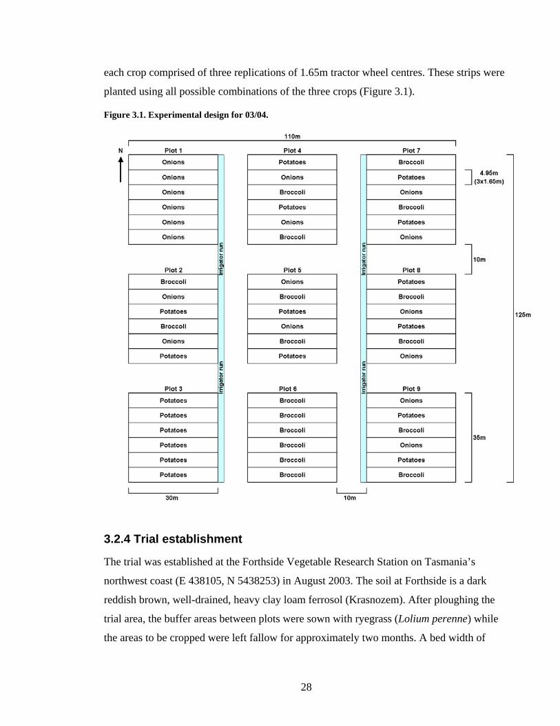
28
each crop comprised of three replications of 1.65m tractor wheel centres. These strips were
planted using all possible combinations of the three crops (Figure 3.1).
Figure 3.1. Experimental design for 03/04.
3.2.4 Trial establishment
The trial was established at the Forthside Vegetable Research Station on Tasmania’s
northwest coast (E 438105, N 5438253) in August 2003. The soil at Forthside is a dark
reddish brown, well-drained, heavy clay loam ferrosol (Krasnozem). After ploughing the
trial area, the buffer areas between plots were sown with ryegrass (Lolium perenne) while
the areas to be cropped were left fallow for approximately two months. A bed width of

29
1.65m was used to match the 1.65m wheel centres of the tractors and other equipment at the
research farm. On 10 September 2003, each plot was marked out with white pegs placed in
the middle of the first bed at both ends of each crop strip (the first of three beds) for the
tractor operator to line up with in order to keep the beds straight. To maintain simplicity
each crop type was managed separately using conventional district practices.
Due to the large scale of the experiment, irrigation was applied using a travelling irrigator,
which is also standard industry practice for the region. Again to maintain management
simplicity, irrigation scheduling was based on Class A Pan derived water use estimates and
not individual crop requirements. To improve application uniformity the irrigator was set
up to perform two runs over the experimental area, the first run was in a line along the edge
of Plots 7, 8 and 9, and the second run was in a line along the edge of Plots 1, 2 and 3 .
3.2.5 Monitoring of crops for pests and diseases
Each crop was monitored for pests and diseases on a regular basis. Commercial practice
typically involves the use of chemical disease protectants and insect management strategies,
which aim to maintain diseases and insect pests at negligible levels. However, for the
purposes of this experiment, higher than commercial pest and disease thresholds were
adopted in order to determine if the strip cropping plots were more or less robust than
single species plantings.
3.2.6 Onion management and data collection
Onions (Allium cepa L. cv. Cream Gold) were planted on 30 September 2003, with
13:14:13 NPK fertiliser at the rate of 650kg/ha, in eight rows per bed with a target density
of approximately 60-80 plants/m2 in line with industry practice (Boersma M., Agronomist,
Field Fresh Pty Ltd, pers. comm. 2003)(Picture 3.1).

30
Picture 3.1. Onions planted into three beds per strip with 8 rows of onions per bed.
Weeds were controlled with herbicides according to standard commercial practice, using a
modified sprayer with a five-metre boom, which equates to three tractor widths (the design
and use of this sprayer is discussed in Chapter 6). The chemical applications were: 26
November Tramat® (ethofumesate 1 kg a.i./ha); 4 December Tribunil®
(methabenzthiazuron 1.05kg a.i./ha) and Totril® (ioxynil 0.375kg a.i./ha); 9 December
Tribunil® (methabenzthiazuron 1.05kg a.i./ha) and Totril® (ioxynil 0.375kg a.i./ha). The
onions were lifted on the 4 April 2004 in order for the bulbs and blades to dry and the skins
to harden before harvest on 20 April 2004 (Picture 3.2).
Picture 3.2. Onions after lifting.
Each bed (tractor width) was randomly sampled using a 0.5m2 quadrat. Two quadrats were
taken for each bag and there were three bags to each bed (3m2)(Picture 3.3 and Picture3.4).
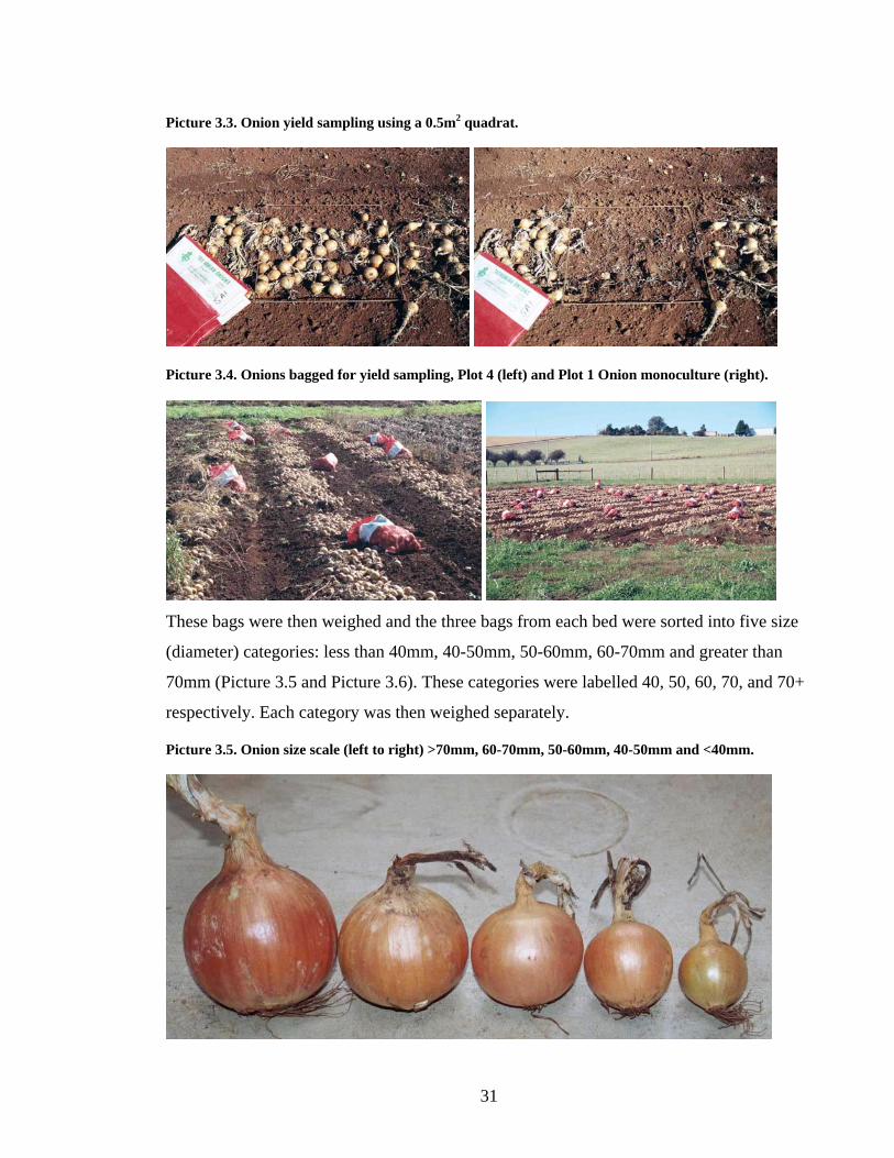
31
Picture 3.3. Onion yield sampling using a 0.5m2 quadrat.
Picture 3.4. Onions bagged for yield sampling, Plot 4 (left) and Plot 1 Onion monoculture (right).
These bags were then weighed and the three bags from each bed were sorted into five size
(diameter) categories: less than 40mm, 40-50mm, 50-60mm, 60-70mm and greater than
70mm (Picture 3.5 and Picture 3.6). These categories were labelled 40, 50, 60, 70, and 70+
respectively. Each category was then weighed separately.
Picture 3.5. Onion size scale (left to right) >70mm, 60-70mm, 50-60mm, 40-50mm and <40mm.
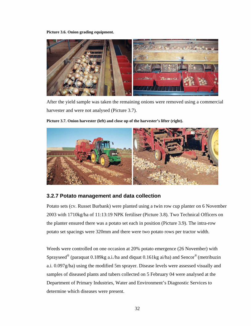
32
Picture 3.6. Onion grading equipment.
After the yield sample was taken the remaining onions were removed using a commercial
harvester and were not analysed (Picture 3.7).
Picture 3.7. Onion harvester (left) and close up of the harvester’s lifter (right).
3.2.7 Potato management and data collection
Potato sets (cv. Russet Burbank) were planted using a twin row cup planter on 6 November
2003 with 1710kg/ha of 11:13:19 NPK fertiliser (Picture 3.8). Two Technical Officers on
the planter ensured there was a potato set each in position (Picture 3.9). The intra-row
potato set spacings were 320mm and there were two potato rows per tractor width.
Weeds were controlled on one occasion at 20% potato emergence (26 November) with
Sprayseed® (paraquat 0.189kg a.i./ha and diquat 0.161kg ai/ha) and Sencor® (metribuzin
a.i. 0.097g/ha) using the modified 5m sprayer. Disease levels were assessed visually and
samples of diseased plants and tubers collected on 5 February 04 were analysed at the
Department of Primary Industries, Water and Environment’s Diagnostic Services to
determine which diseases were present.
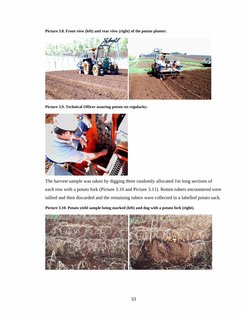
33
Picture 3.8. Front view (left) and rear view (right) of the potato planter.
Picture 3.9. Technical Officer assuring potato set regularity.
The harvest sample was taken by digging three randomly allocated 1m long sections of
each row with a potato fork (Picture 3.10 and Picture 3.11). Rotten tubers encountered were
tallied and then discarded and the remaining tubers were collected in a labelled potato sack.
Picture 3.10. Potato yield sample being marked (left) and dug with a potato fork (right).

34
Picture 3.11. Technical officer taking potato yield samples.
The samples were weighed and then graded, using commercial specifications into different
size ranges (850g-250g; 250g-75g; and 75g and less). The tubers were then washed and any
tubers with defects were removed and weighed. The potatoes remaining in the field were
harvested using a commercial harvester and not analysed.
3.2.8 Broccoli management and data collection
Broccoli Speedlings (Brassica oleracea var. italica cv. Green Belt) were transplanted on 11
November 2003 with 500kg/ha of 14:14:12 NPK fertiliser including 1% boron, using a 6-
row transplanter (Picture 3.12). The Speedlings were transplanted in two rows per 1.65m
bed in a 300mm x 800mm grid, with 300mm between plants and 800mm between rows.
Picture 3.12. Six row broccoli transplanter, rear view (left) front view (right).
Using the 6-row planter meant that one entire strip (three 1.65m beds) could be planted in
one pass. The monoculture plot (Plot 6) was planted first in order to ensure that any
planting problems were resolved before broccoli was transplanted in the strip cropping
plots between onions and potatoes.
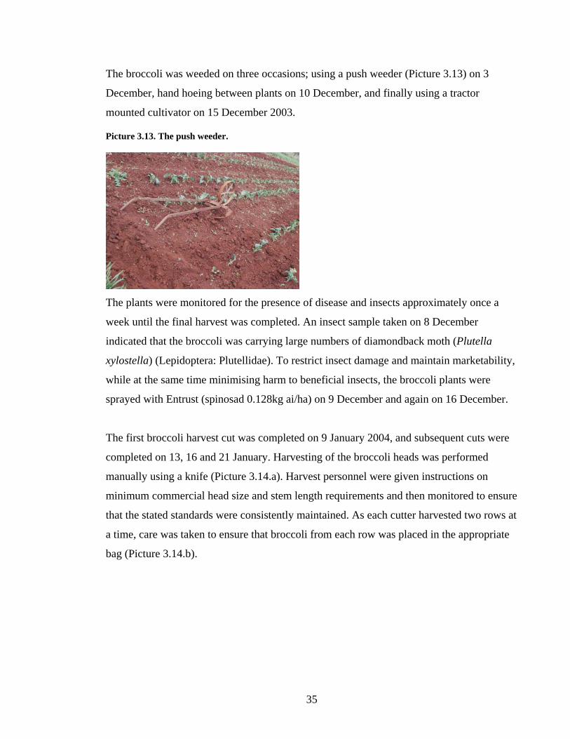
35
The broccoli was weeded on three occasions; using a push weeder (Picture 3.13) on 3
December, hand hoeing between plants on 10 December, and finally using a tractor
mounted cultivator on 15 December 2003.
Picture 3.13. The push weeder.
The plants were monitored for the presence of disease and insects approximately once a
week until the final harvest was completed. An insect sample taken on 8 December
indicated that the broccoli was carrying large numbers of diamondback moth (Plutella
xylostella) (Lepidoptera: Plutellidae). To restrict insect damage and maintain marketability,
while at the same time minimising harm to beneficial insects, the broccoli plants were
sprayed with Entrust (spinosad 0.128kg ai/ha) on 9 December and again on 16 December.
The first broccoli harvest cut was completed on 9 January 2004, and subsequent cuts were
completed on 13, 16 and 21 January. Harvesting of the broccoli heads was performed
manually using a knife (Picture 3.14.a). Harvest personnel were given instructions on
minimum commercial head size and stem length requirements and then monitored to ensure
that the stated standards were consistently maintained. As each cutter harvested two rows at
a time, care was taken to ensure that broccoli from each row was placed in the appropriate
bag (Picture 3.14.b).
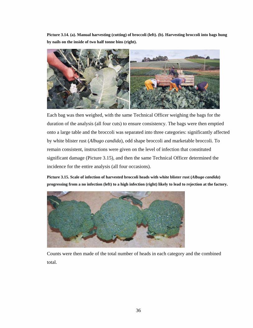
36
Picture 3.14. (a). Manual harvesting (cutting) of broccoli (left). (b). Harvesting broccoli into bags hung
by nails on the inside of two half tonne bins (right).
Each bag was then weighed, with the same Technical Officer weighing the bags for the
duration of the analysis (all four cuts) to ensure consistency. The bags were then emptied
onto a large table and the broccoli was separated into three categories: significantly affected
by white blister rust (Albugo candida), odd shape broccoli and marketable broccoli. To
remain consistent, instructions were given on the level of infection that constituted
significant damage (Picture 3.15), and then the same Technical Officer determined the
incidence for the entire analysis (all four occasions).
Picture 3.15. Scale of infection of harvested broccoli heads with white blister rust (Albugo candida)
progressing from a no infection (left) to a high infection (right) likely to lead to rejection at the factory.
Counts were then made of the total number of heads in each category and the combined
total.

37
3.2.9 Data analysis
The data were analysed with a one-way analysis of variance (ANOVA) using the general
linear model (Proc GLM) of SAS v8.2 (SAS Institute, Cary, NC). The various mean counts
from each crop row were used as the response variables, while the plot and the
neighbouring plant row were the predictor variables. A sample analysis is presented as an
appendix. Statistically significant treatment means (P < 0.05) were separated using Fisher’s
least significant difference (LSD). Data were log +1 transformed when necessary to
conform to the assumptions of the ANOVA procedure. Data expressed as proportions were
first arcsine square root transformed before analysis. However, only non-transformed
means were reported, except where otherwise noted.
To determine the treatment effects of strip cropping, pairwise contrasts were planned.
These contrasts compared the results from the monoculture plots with the results from rows
of plants grown immediately adjacent to rows of other crop types, the plants growing
immediately adjacent to the plot edges and the rows in the middle of the strip cropping
plots. In the case of potatoes and broccoli the six row strips were broken up in the following
manner: left and right outer edge rows, left and right inner edge row, two middle rows,
inner edge row and outer edge row. Schematic representations of the naming of rows within
a potato strip in the middle of a plot and on the edge of a plot are presented in Figure 3.2. A
similar naming protocol was applied to the equivalent broccoli rows.
Figure 3.2. Schematic of naming of a middle 4.95m potato strip cropping strip (left) and a schematic of
a 4.95m potato strip cropping strip on a plot edge (right).
Bro
ccol
i str
ip
Out
er b
rocc
oli e
dge
row
Inne
r oni
on e
dge
row
Out
er o
nion
edg
e ro
w
Oni
on s
trip
Inne
rbro
ccol
i edg
e ro
w
Mid
dle
row
Mid
dle
row
Inne
r plo
t edg
e ro
w
Out
er p
lot e
dge
row
Plot
edg
e
Mid
dle
row
Bro
ccol
i str
ip
Out
er b
rocc
oli e
dge
row
Inne
r bro
ccol
i edg
e ro
w
Mid
dle
row

38
The following pairwise contrasts were planned for the potato results:
1. Both inner and outer broccoli edge rows vs. Potato monoculture
2. Outer broccoli edge rows vs. Potato monoculture
3. Both outer and inner onion edge rows vs. Potato monoculture
4. Outer onion edge rows vs. Potato monoculture
5. Both outer and inner plot edge rows vs. Potato monoculture
6. Outer plot edge rows vs. Potato monoculture
7. Both middle strip cropping rows vs. Potato monoculture
8. All strip cropped potato rows vs. Potato monoculture
The following contrasts were planned for the broccoli results:
1. Both inner and outer potato edge rows vs. Broccoli monoculture
2. Outer potato edge rows vs. Broccoli monoculture
3. Both inner and outer onion edge rows vs. Broccoli monoculture
4. Outer onion edge rows vs. Broccoli monoculture
5. Both inner and outer plot edge rows vs. Broccoli monoculture
6. Outer plot edge rows vs. Broccoli monoculture
7. Both middle strip cropping rows vs. Broccoli monoculture
8. All strip cropped broccoli rows vs. Broccoli monoculture
An inability to separate individual onion rows due to the mechanical lifting of each onion
bed to allow in situ drying and maturation of the bulbs, restricted the analysis of the onion
results to the 1.65m bed level. This resulted in a reduction in the number of possible
pairwise contrasts and the breakdown of the strips into outer edge row, middle rows and
outer edge row. A schematic of this naming process is represented in Figure 3.3.

39
Figure 3.3. Schematic of naming of a middle 4.95m onion strip cropping strip (left) and a schematic of a
4.95m onion strip cropping strip on a plot edge (right).
Therefore the following contrasts were planned:
1. Broccoli edge rows vs. Onion monoculture
2. Potato edge rows vs. Onion monoculture
3. Plot edge rows vs. Onion monoculture
4. Middle strip cropping rows vs. Onion monoculture
Example ANOVA tables are presented as appendices.
3.3 Results
3.3.1 Meteorological data
The only significant difference between the long-term climatic averages and the 03/04
season was the above average rainfall total in January followed by below average rainfall in
February and March (Table 3.4).
Table 3.4. Mean monthly meteorological data for Forthside from September to March in 03/04 with
long term averages in brackets.
Month - Year Min. Temp. (degC) Max. Temp. (degC) Rainfall Total (mm)
September-03 4.8 (4.9) 12.9 (13.3) 117.8 (98.3)
October-03 5.8 (6.2) 14.6 (15.4) 32.2 (84.9)
November-03 9.3 (8.1) 18.1 (17.1) 21.6 (69.5)
December-03 11.5 (9.6) 20.6 (18.9) 73.6 (67.5)
January-04 10.4 (11.0) 20.1 (20.6) 161.7 (54.4)
February-04 12.0 (11.6) 21.4 (21.0) 13.7 (45.8)
March-04 10.0 (10.4) 20.0 (19.8) 31.0 (55.5)
Bro
ccol
i str
ip
Bro
ccol
i edg
e ro
w
Pota
to s
trip
Mid
dle
row
Pota
to e
dge
row
Bro
ccol
i str
ip
Bro
ccol
i edg
e ro
w
Mid
dle
row
Plot
edg
e
Plot
edg
e ro
w
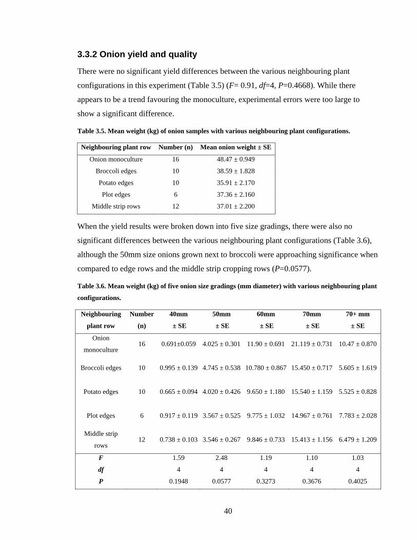
40
3.3.2 Onion yield and quality
There were no significant yield differences between the various neighbouring plant
configurations in this experiment (Table 3.5) (F= 0.91, df=4, P=0.4668). While there
appears to be a trend favouring the monoculture, experimental errors were too large to
show a significant difference.
Table 3.5. Mean weight (kg) of onion samples with various neighbouring plant configurations.
Neighbouring plant row Number (n) Mean onion weight ± SE
Onion monoculture 16 48.47 ± 0.949
Broccoli edges 10 38.59 ± 1.828
Potato edges 10 35.91 ± 2.170
Plot edges 6 37.36 ± 2.160
Middle strip rows 12 37.01 ± 2.200
When the yield results were broken down into five size gradings, there were also no
significant differences between the various neighbouring plant configurations (Table 3.6),
although the 50mm size onions grown next to broccoli were approaching significance when
compared to edge rows and the middle strip cropping rows (P=0.0577).
Table 3.6. Mean weight (kg) of five onion size gradings (mm diameter) with various neighbouring plant
configurations.
Neighbouring
plant row
Number
(n)
40mm
± SE
50mm
± SE
60mm
± SE
70mm
± SE
70+ mm
± SE
Onion
monoculture 16 0.691±0.059 4.025 ± 0.301 11.90 ± 0.691 21.119 ± 0.731 10.47 ± 0.870
Broccoli edges 10 0.995 ± 0.139 4.745 ± 0.538 10.780 ± 0.867 15.450 ± 0.717 5.605 ± 1.619
Potato edges 10 0.665 ± 0.094 4.020 ± 0.426 9.650 ± 1.180 15.540 ± 1.159 5.525 ± 0.828
Plot edges 6 0.917 ± 0.119 3.567 ± 0.525 9.775 ± 1.032 14.967 ± 0.761 7.783 ± 2.028
Middle strip
rows 12 0.738 ± 0.103 3.546 ± 0.267 9.846 ± 0.733 15.413 ± 1.156 6.479 ± 1.209
F 1.59 2.48 1.19 1.10 1.03
df 4 4 4 4 4
P 0.1948 0.0577 0.3273 0.3676 0.4025

41
Similarly, the planned contrasts of the yield results (Table 3.7) did not reveal any
significant differences between onions grown in monoculture and strip cropped onions in
different neighbouring plant configurations.
Table 3.7. Planned pairwise contrasts of neighbouring plant configurations and onions grown in
monoculture (df=1).
Contrast F P
Broccoli edges vs. Onion monoculture 1.33 0.2546
Potato edges vs. Onion monoculture 2.44 0.1255
Plot edges vs. Onion monoculture 2.86 0.0980
Strip middle rows vs. Onion monoculture 1.74 0.1946
Strip cropping vs. Monoculture 1.94 0.1704
When these planned contrasts were performed on the five different size gradings (Table
3.8), onions grown in the monoculture produced significantly more than the plot edges in
the 60mm and 70mm size ranges (P=0.0469 and P=0.0450 respectively).
Table 3.8. Planned pairwise contrasts of five different size gradings of neighbouring plant
configurations and onions grown in monoculture (df=1). Significant results are shown in bold type.
40mm ± SE 50mm ± SE 60mm ± SE 70mm ± SE 70+mm ± SE Contrast
F P F P F P F P F P
Broccoli edges vs. Onion
monoculture 0.04 0.8432 0.01 0.9253 1.84 0.1825 2.89 0.0961 0.98 0.3286
Potato edges vs. Onion
monoculture 0.48 0.4929 0.31 0.5804 2.57 0.1162 2.41 0.1278 0.71 0.4052
Plot edges vs. Onion
monoculture 0.18 0.6724 2.1 0.1549 4.19 0.0469 4.26 0.0450 2.56 0.1167
Strip middle rows vs. Onion
monoculture 0.39 0.5364 1.68 0.2022 2.93 0.0941 2.45 0.1251 1.9 0.1749
Strip cropping vs.
Monoculture 0.15 0.7026 0.45 0.5068 2.60 0.1141 2.77 0.1032 1.23 0.2744
The biggest difference in the onion yield results and the planned contrasts was a very
significant plot effect (F=8.13, df=6, P<0.0001). The mean onion sample data from each
plot (Table 3.9) illustrates that the harvest yields were not evenly distributed across the trial
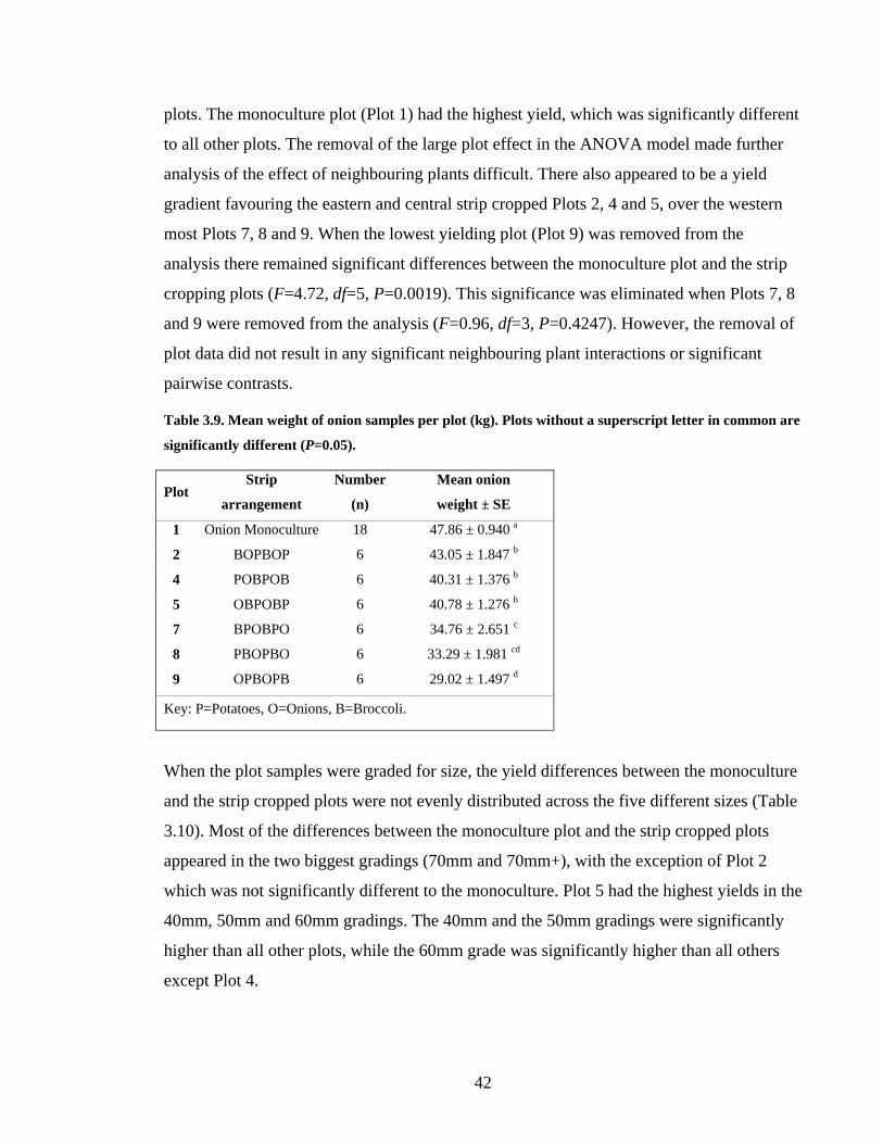
42
plots. The monoculture plot (Plot 1) had the highest yield, which was significantly different
to all other plots. The removal of the large plot effect in the ANOVA model made further
analysis of the effect of neighbouring plants difficult. There also appeared to be a yield
gradient favouring the eastern and central strip cropped Plots 2, 4 and 5, over the western
most Plots 7, 8 and 9. When the lowest yielding plot (Plot 9) was removed from the
analysis there remained significant differences between the monoculture plot and the strip
cropping plots (F=4.72, df=5, P=0.0019). This significance was eliminated when Plots 7, 8
and 9 were removed from the analysis (F=0.96, df=3, P=0.4247). However, the removal of
plot data did not result in any significant neighbouring plant interactions or significant
pairwise contrasts.
Table 3.9. Mean weight of onion samples per plot (kg). Plots without a superscript letter in common are
significantly different (P=0.05).
Plot Strip
arrangement
Number
(n)
Mean onion
weight ± SE
1 Onion Monoculture 18 47.86 ± 0.940 a
2 BOPBOP 6 43.05 ± 1.847 b
4 POBPOB 6 40.31 ± 1.376 b
5 OBPOBP 6 40.78 ± 1.276 b
7 BPOBPO 6 34.76 ± 2.651 c
8 PBOPBO 6 33.29 ± 1.981 cd
9 OPBOPB 6 29.02 ± 1.497 d
Key: P=Potatoes, O=Onions, B=Broccoli.
When the plot samples were graded for size, the yield differences between the monoculture
and the strip cropped plots were not evenly distributed across the five different sizes (Table
3.10). Most of the differences between the monoculture plot and the strip cropped plots
appeared in the two biggest gradings (70mm and 70mm+), with the exception of Plot 2
which was not significantly different to the monoculture. Plot 5 had the highest yields in the
40mm, 50mm and 60mm gradings. The 40mm and the 50mm gradings were significantly
higher than all other plots, while the 60mm grade was significantly higher than all others
except Plot 4.

43
Table 3.10. Mean weight (kg) of five onion size gradings (diameter in mm) per plot. Significant results
are shown in bold type. Plots in grading columns without a superscript letter in common are
significantly different (P=0.05).
Plot Strip
arrangement
Number
(n)
40mm
± SE
50mm
± SE
60mm
± SE
70mm
± SE
70+ mm
± SE
1 Monoculture 18 0.70 ± 0.053 bc 3.91 ± 0.290 bc 11.54 ± 0.66 b 20.67 ± 0.712 a 10.84 ± 0.811 a
2 BOPBOP 6 0.70 ± 0.081 bc 2.93 ± 0.221 cd 7.42 ± 0.40 c 18.83 ± 0.649 ab 12.38 ± 1.608 a
4 POBPOB 6 0.87 ± 0.138 b 4.67 ± 0.336 b 11.83 ± 0.77 ab 17.46 ± 0.761 bc 4.48 ± 0.604 bc
5 OBPOBP 6 1.28 ± 0.194 a 5.73 ± 0.540 a 14.01 ± 0.44 a 16.04 ± 1.053 cd 2.93 ± 0.571 c
7 BPOBPO 6 0.68 ± 0.099 bc 4.34 ± 0.328 b 10.80 ± 0.89 b 14.45 ± 1.114 de 3.73 ± 0.655 bc
8 PBOPBO 6 0.94 ± 0.092 b 4.18 ± 0.306 b 9.93 ± 0.59 b 12.96 ± 0.944 e 4.48 ± 0.795 bc
9 OPBOPB 6 0.44 ± 0.068 c 2.41 ± 0.239 d 6.63 ± 0.53 c 11.96 ± 0.762 e 6.69 ± 0.930 b
F 5.17 8.13 8.85 5.72 10.32
df 6 6 6 6 6
P 0.0004 <0.0001 <0.0001 0.0002 <0.0001
Key: P=Potatoes, O=Onions, B=Broccoli.
3.3.3 Potato yield and quality
There were no significant differences in potato yields between the various neighbouring
plant configurations (Table 3.11) (F=0.78, df=7, P=0.6096).
Table 3.11. Mean weight (kg) of potato samples with various neighbouring plant configurations.
Neighbouring
plant
Number
(n)
Mean potato
weight (kg) ± SE
Potato monoculture 32 12.41 ± 1.532
Outer broccoli edges 10 10.87 ± 1.149
Inner broccoli edges 10 14.46 ± 1.602
Outer onion edges 10 13.00 ± 1.013
Inner onion edges 10 11.58 ± 0.968
Outer plot edges 6 13.68 ± 1.311
Inner plot edges 6 13.38 ± 1.446
Middle strip rows 24 15.24 ± 0.362
For processing potatoes like Russet Burbanks, tubers in the 850g-250g size range are
considered to be “premium” tubers, while the 250g-75g are considered to be of processing

44
size and tubers under 75g are unacceptable and grouped as “rejects” together with tubers
that exhibit some form of defect. When the potato yield results were partitioned into these
three categories (Table 3.12), there were no significant yield differences between the
various neighbouring plant configurations.
Table 3.12. Mean weight (kg) of three potato quality categories with various neighbouring plant
configurations.
Neighbouring plant Number (n) 850g-250g 250g-75g Rejects
Potato monoculture 32 7.001 ± 0.259 7.142 ± 0.301 1.635 ± 0.103
Outer broccoli edges 10 5.488 ± 1.196 6.004 ± 0.569 2.288 ± 0.252
Inner broccoli edges 10 4.750 ± 0.832 5.162 ± 0.339 1.625 ± 0.308
Outer onion edges 10 6.372 ± 0.848 6.430 ± 0.616 1.736 ± 0.233
Inner onion edges 10 5.800 ± 0.834 6.549 ± 0.868 1.739 ± 0.227
Outer plot edges 6 6.647 ± 0.959 6.868 ± 1.135 1.896 ± 0.133
Inner plot edges 6 6.473 ± 0.520 5.664 ± 0.870 1.915 ± 0.346
Middle strip rows 24 5.495 ± 0.483 5.116 ± 0.539 2.170 ± 0.221
F 0.32 0.97 1.15
df 7 7 7
P 0.9437 0.4608 0.3407
When the reasons for the rejections were ranked from one to four, with one being the defect
with the lowest incidence in the sample and four being the defect with the highest incidence
(Table 3.13), there were no significant differences between the defects, “small”, “green”
and “knobby”. The five other rejection defects, “hollow”, “rot”, “grub”, “cracks” and
“damage” were too infrequent to be analysed.

45
Table 3.13. Mean weight (kg) of potato rejection categories with various neighbouring plant
configurations.
Neighbouring plant Number (n) Small ± SE Green ± SE Knobby ± SE
Potato monoculture 32 2.406 ± 0.287 2.125 ± 0.245 1.531 ± 0.273
Outer broccoli edges 10 1.200 ± 0.611 3.300 ± 0.213 2.200 ± 0.291
Inner broccoli edges 10 2.500 ± 0.543 2.900 ± 0.379 1.600 ± 0.499
Outer onion edges 10 2.000 ± 0.577 2.400 ± 0.221 2.100 ± 0.504
Inner onion edges 10 2.200 ± 0.533 2.800 ± 0.249 1.700 ± 0.539
Outer plot edges 6 2.333 ± 0.667 3.000 ± 0.365 0.833 ± 0.654
Inner plot edges 6 2.333 ± 0.760 3.000 ± 0.516 1.500 ± 0.563
Middle strip rows 24 1.708 ± 0.316 2.917 ± 0.255 2.292 ± 0.237
F 0.67 1.31 0.81
df 7 7 7
P 0.6980 0.2523 0.5816
Planned contrasts of the potato yields did not reveal any significant differences between
potatoes grown in monoculture and strip cropped potatoes in different neighbouring plant
configurations (Table 3.14).
Table 3.14. Planned pairwise contrasts of various neighbouring plant configurations and potatoes
grown in monoculture (df=1).
Contrast F P
Both broccoli edge rows vs. Potato monoculture 0.23 0.6294
Outer broccoli edge rows vs. Potato monoculture 0.01 0.9117
Both onion edge rows vs. Potato monoculture 0.00 0.9959
Outer onion edge rows vs. Potato monoculture 0.01 0.9429
Both plot edge rows vs. Potato monoculture 0.18 0.6734
Outer plot edge rows vs. Potato monoculture 0.00 0.9803
Middle strip rows vs. Potato monoculture 0.64 0.4255
Strip Cropping vs. Monoculture 0.13 0.7175
Planned contrasts of the three different quality categories (Table 3.15) also resulted in no
significant differences between potatoes grown in monoculture and potatoes grown in
various neighbouring plant configurations.
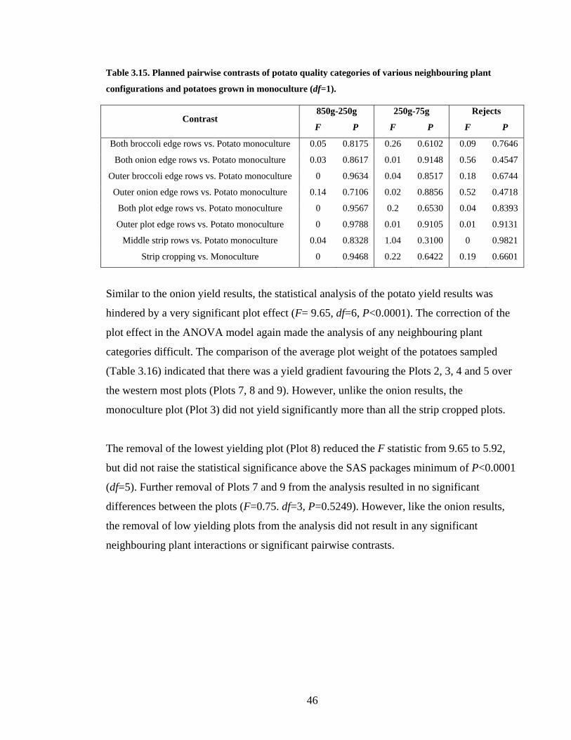
46
Table 3.15. Planned pairwise contrasts of potato quality categories of various neighbouring plant
configurations and potatoes grown in monoculture (df=1).
850g-250g 250g-75g Rejects Contrast
F P F P F P
Both broccoli edge rows vs. Potato monoculture 0.05 0.8175 0.26 0.6102 0.09 0.7646
Both onion edge rows vs. Potato monoculture 0.03 0.8617 0.01 0.9148 0.56 0.4547
Outer broccoli edge rows vs. Potato monoculture 0 0.9634 0.04 0.8517 0.18 0.6744
Outer onion edge rows vs. Potato monoculture 0.14 0.7106 0.02 0.8856 0.52 0.4718
Both plot edge rows vs. Potato monoculture 0 0.9567 0.2 0.6530 0.04 0.8393
Outer plot edge rows vs. Potato monoculture 0 0.9788 0.01 0.9105 0.01 0.9131
Middle strip rows vs. Potato monoculture 0.04 0.8328 1.04 0.3100 0 0.9821
Strip cropping vs. Monoculture 0 0.9468 0.22 0.6422 0.19 0.6601
Similar to the onion yield results, the statistical analysis of the potato yield results was
hindered by a very significant plot effect (F= 9.65, df=6, P<0.0001). The correction of the
plot effect in the ANOVA model again made the analysis of any neighbouring plant
categories difficult. The comparison of the average plot weight of the potatoes sampled
(Table 3.16) indicated that there was a yield gradient favouring the Plots 2, 3, 4 and 5 over
the western most plots (Plots 7, 8 and 9). However, unlike the onion results, the
monoculture plot (Plot 3) did not yield significantly more than all the strip cropped plots.
The removal of the lowest yielding plot (Plot 8) reduced the F statistic from 9.65 to 5.92,
but did not raise the statistical significance above the SAS packages minimum of P<0.0001
(df=5). Further removal of Plots 7 and 9 from the analysis resulted in no significant
differences between the plots (F=0.75. df=3, P=0.5249). However, like the onion results,
the removal of low yielding plots from the analysis did not result in any significant
neighbouring plant interactions or significant pairwise contrasts.

47
Table 3.16. Mean weight of the potato samples per plot (kg). Plots without a superscript letter in
common are significantly different (P=0.05).
Plot Strip
arrangement Number (n)
Mean potato
weight (kg)
2 BOPBOP 12 14.969 ± 0.833 a
3 Monoculture 36 15.164 ± 0.343 a
4 POBPOB 12 15.740 ± 0.822 a
5 OBPOBP 12 13.957 ± 0.868 a
7 BPOBPO 12 10.519 ± 1.067 b
8 PBOPBO 12 7.698 ± 1.040 c
9 OPBOPB 12 11.111 ± 1.082 b
Key: P=Potatoes, O=Onions, B=Broccoli.
The size range plot data indicated that the plots that yielded the most (Strip cropping Plots
2, 4 and 5; and the Plot 3 monoculture) did so by producing the most premium sized tubers
i.e. 850g-250g (Table 3.17).
Table 3.17 Mean plot weights (kg) of three potato quality categories. Significant results are shown in
bold type. Plots in category columns without a superscript letter in common are significantly different
(P=0.05).
Plot Strip
arrangement Number (n) 850g-250g ± SE 250g-75g ± SE Rejects ± SE
2 BOPBOP 12 6.737 ± 0.432 a 6.928 ± 0.562 a 2.310 ± 0.374 ab
3 Monoculture 36 6.994 ± 0.252 a 7.089 ± 0.270a 1.626 ± 0.096 bc
4 POBPOB 12 8.117 ± 0.681 a 6.579 ± 0.489 a 2.119 ± 0.184 ab
5 OBPOBP 12 6.870 ± 0.617 a 6.143 ± 0.708 ab 2.456 ± 0.261 a
7 BPOBPO 12 4.932 ± 0.628 b 4.927 ± 0.514 bc 1.533 ± 0.173 c
8 PBOPBO 12 3.490 ± 0.583 b 3.534 ± 0.629 c 1.486 ± 0.154 c
9 OPBOPB 12 3.765 ± 0.579 b 6.284 ± 0.713 ab 1.981 ± 0.257 ab
F 8.93 4.06 2.84
df 6 6 6
P <0.0001 <0.0001 0.0139
Key: P=Potatoes, O=Onions, B=Broccoli.
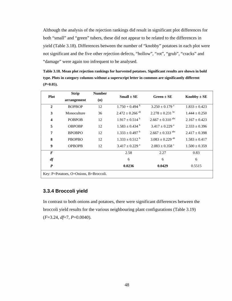
48
Although the analysis of the rejection rankings did result in significant plot differences for
both “small” and “green” tubers, these did not appear to be related to the differences in
yield (Table 3.18). Differences between the number of “knobby” potatoes in each plot were
not significant and the five other rejection defects, “hollow”, “rot”, “grub”, “cracks” and
“damage” were again too infrequent to be analysed.
Table 3.18. Mean plot rejection rankings for harvested potatoes. Significant results are shown in bold
type. Plots in category columns without a superscript letter in common are significantly different
(P=0.05).
Plot Strip
arrangement
Number
(n) Small ± SE Green ± SE Knobby ± SE
2 BOPBOP 12 1.750 + 0.494 b 3.250 ± 0.179 a 1.833 ± 0.423
3 Monoculture 36 2.472 ± 0.266 ab 2.278 ± 0.231 bc 1.444 ± 0.250
4 POBPOB 12 1.917 ± 0.514 b 2.667 ± 0.310 abc 2.167 ± 0.423
5 OBPOBP 12 1.583 ± 0.434 b 3.417 ± 0.229 a 2.333 ± 0.396
7 BPOBPO 12 1.333 ± 0.497 b 2.667 ± 0.333 abc 2.417 ± 0.398
8 PBOPBO 12 1.333 ± 0.512 b 3.083 ± 0.229 ab 1.583 ± 0.417
9 OPBOPB 12 3.417 ± 0.229 a 2.083 ± 0.358 c 1.500 ± 0.359
F 2.58 2.27 0.83
df 6 6 6
P 0.0236 0.0429 0.5515
Key: P=Potatoes, O=Onions, B=Broccoli.
3.3.4 Broccoli yield
In contrast to both onions and potatoes, there were significant differences between the
broccoli yield results for the various neighbouring plant configurations (Table 3.19)
(F=3.24, df=7, P=0.0040).
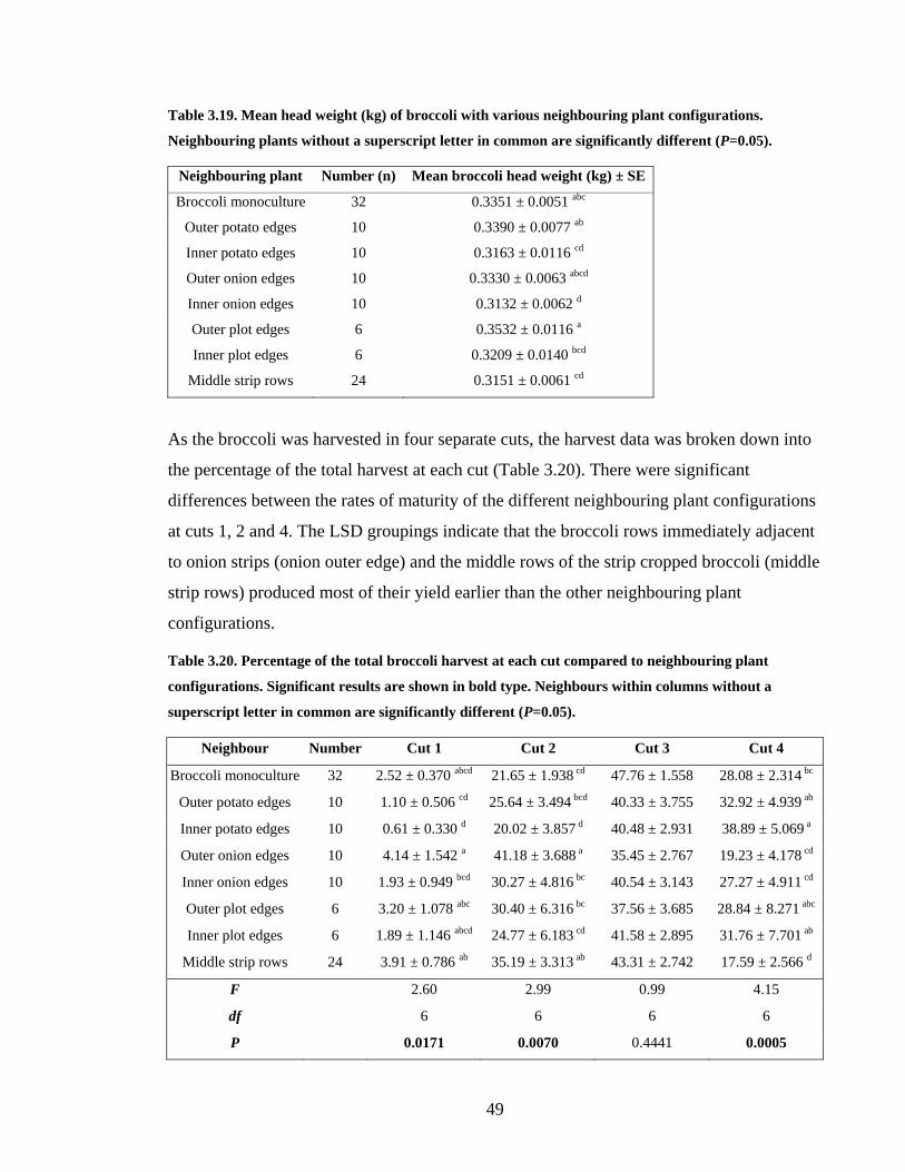
49
Table 3.19. Mean head weight (kg) of broccoli with various neighbouring plant configurations.
Neighbouring plants without a superscript letter in common are significantly different (P=0.05).
Neighbouring plant Number (n) Mean broccoli head weight (kg) ± SE
Broccoli monoculture 32 0.3351 ± 0.0051 abc
Outer potato edges 10 0.3390 ± 0.0077 ab
Inner potato edges 10 0.3163 ± 0.0116 cd
Outer onion edges 10 0.3330 ± 0.0063 abcd
Inner onion edges 10 0.3132 ± 0.0062 d
Outer plot edges 6 0.3532 ± 0.0116 a
Inner plot edges 6 0.3209 ± 0.0140 bcd
Middle strip rows 24 0.3151 ± 0.0061 cd
As the broccoli was harvested in four separate cuts, the harvest data was broken down into
the percentage of the total harvest at each cut (Table 3.20). There were significant
differences between the rates of maturity of the different neighbouring plant configurations
at cuts 1, 2 and 4. The LSD groupings indicate that the broccoli rows immediately adjacent
to onion strips (onion outer edge) and the middle rows of the strip cropped broccoli (middle
strip rows) produced most of their yield earlier than the other neighbouring plant
configurations.
Table 3.20. Percentage of the total broccoli harvest at each cut compared to neighbouring plant
configurations. Significant results are shown in bold type. Neighbours within columns without a
superscript letter in common are significantly different (P=0.05).
Neighbour Number Cut 1 Cut 2 Cut 3 Cut 4
Broccoli monoculture 32 2.52 ± 0.370 abcd 21.65 ± 1.938 cd 47.76 ± 1.558 28.08 ± 2.314 bc
Outer potato edges 10 1.10 ± 0.506 cd 25.64 ± 3.494 bcd 40.33 ± 3.755 32.92 ± 4.939 ab
Inner potato edges 10 0.61 ± 0.330 d 20.02 ± 3.857 d 40.48 ± 2.931 38.89 ± 5.069 a
Outer onion edges 10 4.14 ± 1.542 a 41.18 ± 3.688 a 35.45 ± 2.767 19.23 ± 4.178 cd
Inner onion edges 10 1.93 ± 0.949 bcd 30.27 ± 4.816 bc 40.54 ± 3.143 27.27 ± 4.911 cd
Outer plot edges 6 3.20 ± 1.078 abc 30.40 ± 6.316 bc 37.56 ± 3.685 28.84 ± 8.271 abc
Inner plot edges 6 1.89 ± 1.146 abcd 24.77 ± 6.183 cd 41.58 ± 2.895 31.76 ± 7.701 ab
Middle strip rows 24 3.91 ± 0.786 ab 35.19 ± 3.313 ab 43.31 ± 2.742 17.59 ± 2.566 d
F 2.60 2.99 0.99 4.15
df 6 6 6 6
P 0.0171 0.0070 0.4441 0.0005

50
Several planned pairwise contrasts were significant for the broccoli results (Table 3.21).
The interaction of broccoli and potatoes on the outer potato edge row resulted in broccoli
producing, on average, heavier heads when compared to broccoli grown in monoculture.
However, when the first two potato edge rows were grouped the monoculture produced
heavier broccoli heads, albeit at a lower level of significance. A similar effect was also
evident for the plot edges. Conversely, the first row of broccoli grown next to onions had
significantly smaller average head weights compared to broccoli grown in monoculture,
although this effect did not penetrate into the second edge row. It appears that only the edge
rows exhibited any significant effects because the middle rows and strip cropping in
general were not significantly different from broccoli grown in monoculture. However, the
contrast of monoculture and strip cropping was approaching significance, which would
have resulted in monoculture producing on average head of 0.335 kg compared to strip
cropping producing 0.321kg.
Table 3.21. Planned pairwise contrasts of broccoli yield and the various neighbouring plant
configurations and broccoli grown in monoculture (df=1). Significant results are shown in bold type.
Contrast F P
Both potato edge rows vs. Broccoli monoculture 4.76 0.0317
Outer potato edge rows vs. Broccoli monoculture 7.44 0.0076
Both onion edge rows vs. Broccoli monoculture 3.09 0.0819
Outer onion edge rows vs. Broccoli monoculture 5.03 0.0273
Both plot edge rows vs. Broccoli monoculture 5.97 0.0164
Outer plot edge rows vs. Broccoli monoculture 10.61 0.0016
Middle strip rows vs. Broccoli monoculture 1.90 0.1708
Strip cropping vs. Monoculture 3.68 0.0580
These contrasts were only significant for the pooled harvest data (that is, all four cuts), as
an examination of the planned contrasts at each cut did not show any significant differences
(Table 3.22).
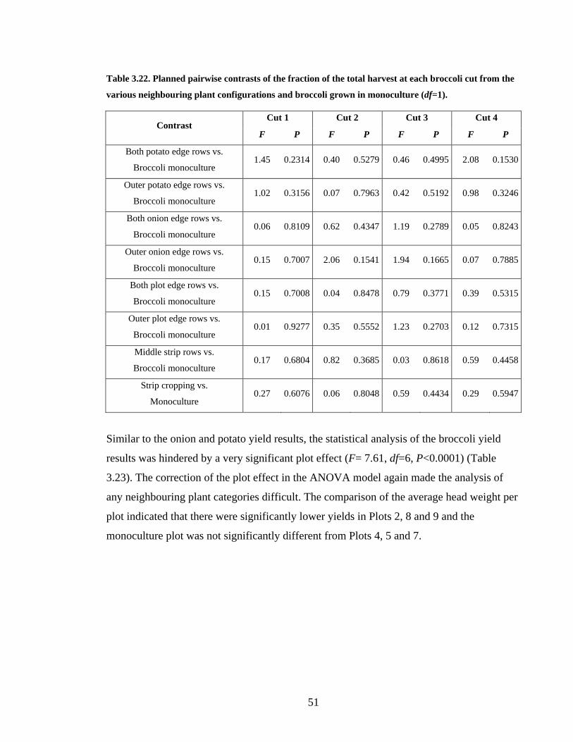
51
Table 3.22. Planned pairwise contrasts of the fraction of the total harvest at each broccoli cut from the
various neighbouring plant configurations and broccoli grown in monoculture (df=1).
Cut 1 Cut 2 Cut 3 Cut 4 Contrast
F P F P F P F P
Both potato edge rows vs.
Broccoli monoculture 1.45 0.2314 0.40 0.5279 0.46 0.4995 2.08 0.1530
Outer potato edge rows vs.
Broccoli monoculture 1.02 0.3156 0.07 0.7963 0.42 0.5192 0.98 0.3246
Both onion edge rows vs.
Broccoli monoculture 0.06 0.8109 0.62 0.4347 1.19 0.2789 0.05 0.8243
Outer onion edge rows vs.
Broccoli monoculture 0.15 0.7007 2.06 0.1541 1.94 0.1665 0.07 0.7885
Both plot edge rows vs.
Broccoli monoculture 0.15 0.7008 0.04 0.8478 0.79 0.3771 0.39 0.5315
Outer plot edge rows vs.
Broccoli monoculture 0.01 0.9277 0.35 0.5552 1.23 0.2703 0.12 0.7315
Middle strip rows vs.
Broccoli monoculture 0.17 0.6804 0.82 0.3685 0.03 0.8618 0.59 0.4458
Strip cropping vs.
Monoculture 0.27 0.6076 0.06 0.8048 0.59 0.4434 0.29 0.5947
Similar to the onion and potato yield results, the statistical analysis of the broccoli yield
results was hindered by a very significant plot effect (F= 7.61, df=6, P<0.0001) (Table
3.23). The correction of the plot effect in the ANOVA model again made the analysis of
any neighbouring plant categories difficult. The comparison of the average head weight per
plot indicated that there were significantly lower yields in Plots 2, 8 and 9 and the
monoculture plot was not significantly different from Plots 4, 5 and 7.

52
Table 3.23. Mean broccoli head weight per plot (kg) ± SE. Plots without a superscript letter in common
are significantly different (P=0.05).
Plot Strip arrangement Number Mean broccoli head weight ± SE
2 BOPBOP 12 0.3142 ± 0.0076 b
4 POBPOB 12 0.3370 ± 0.0057 a
5 OBPOBP 12 0.3400 ± 0.0061 a
6 Monoculture 36 0.3386 ± 0.0051 a
7 BPOBPO 12 0.3358 ± 0.0065 a
8 PBOPBO 12 0.3095 ± 0.0064 bc
9 OPBOPB 12 0.2935 ± 0.0076 c
Key: P=Potatoes, O=Onions, B=Broccoli.
There were also significant plot differences between the rates of maturity at each of the cuts
(Table 3.24). The LSD groupings indicate that Plot 4 was the fastest maturing with the
plot’s highest percentage yield in the second cut, while Plot 9 was the slowest maturing
with the plot’s highest percentage yield coming at the final cut.
Table 3.24. Percentage of the total broccoli harvest at each cut per plot. Significant results are shown in
bold type. Plots within columns without a superscript letter in common are significantly different
(P=0.05).
Plot Strip
arrangement
Number
(n) Cut 1 Cut 2 Cut 3 Cut 4
2 BOPBOP 12 1.93 ± 0.664 bcd 30.14 ± 2.704 b 44.90 ± 2.078 ab 23.03 ± 2.783 bc
4 POBPOB 12 6.65 ± 1.632 a 45.79 ± 4.603 a 32.18 ± 3.985 c 15.38 ± 2.981 c
5 OBPOBP 12 3.60 ± 0.675 b 33.24 ± 3.265 b 46.73 ± 3.172 a 16.43 ± 2.631 c
6 Monoculture 36 2.46 ± 0.331 bc 21.77 ± 1.862 c 47.26 ± 1.468 a 28.50 ± 2.195 b
7 BPOBPO 12 2.63 ± 0.745 bc 36.82 ± 3.947 b 37.69 ± 2.787 bc 22.86 ± 4.334 bc
8 PBOPBO 12 1.18 ± 0.394 cd 29.50 ± 2.719 bc 43.46 ± 2.416 ab 25.86 ± 3.570 b
9 OPBOPB 12 0.19 ± 0.187 d 12.46 ± 2.723 d 37.45 ± 2.801 bc 49.90 ± 4.456 a
F 7.53 9.78 3.26 11.86
df 6 6 6 6
P <0.0001 <0.0001 0.0058 <0.0001
Key: P=Potatoes, O=Onions, B=Broccoli.

53
The removal of the lowest yielding plot (Plot 9) from the pooled harvest data reduced the
significance of the yield difference to P=0.0013 (F=4.40, df=5). The subsequent removal of
all the lower yielding plots (Plots 2, 8 and 9), eliminated the significant difference between
the remaining plots (F=1.06, df=3, P=0.3710) and the neighbouring plant configurations
(F=1.49, df=7, P=0.1863).
Re-analysis of the data with the lowest yielding plots removed, reduced the number of
significant planned contrasts with only the outer edge rows being significantly different to
the broccoli monoculture (Table 3.25).
Table 3.25. Planned pairwise contrasts of various neighbouring plant configurations and broccoli
grown in monoculture with all plots included and with the lowest yielding plots removed (df=1).
Significant results are shown in bold type.
All Plots Plots 2, 8 and
9 removed Contrast
F P F P
Both potato edge rows vs. Broccoli monoculture 4.76 0.0317 3.05 0.0860
Outer potato edge rows vs. Broccoli monoculture 7.44 0.0076 2.98 0.0892
Both onion edge rows vs. Broccoli monoculture 3.09 0.0819 1.41 0.2404
Outer onion edge rows vs. Broccoli monoculture 5.03 0.0273 1.76 0.1897
Both plot edge rows vs. Broccoli monoculture 5.97 0.0164 5.27 0.0252
Outer plot edge rows vs. Broccoli monoculture 10.61 0.0016 8.88 0.0041
Middle strip rows vs. Broccoli monoculture 1.90 0.1708 2.03 0.1595
Strip cropping vs. Monoculture 3.68 0.0580 2.35 0.1304
The low incidence of odd shaped broccoli heads meant that statistical analysis of this defect
was not possible.
3.3.5 Diseases in onions
The onion crop was infected by downy mildew (Peronospora destructor) (Picture 3.16),
which radiated from Plot 5 resulting in significant differences between the infection rates
on each plot (F= 13.02, df=6, P<0.0001)(Table 3.26). Although infection rates were
assessed for each row in the experiment and the location of the infected plants recorded, the
large number of infected plants in Plot 5 made counting the number of infected plants
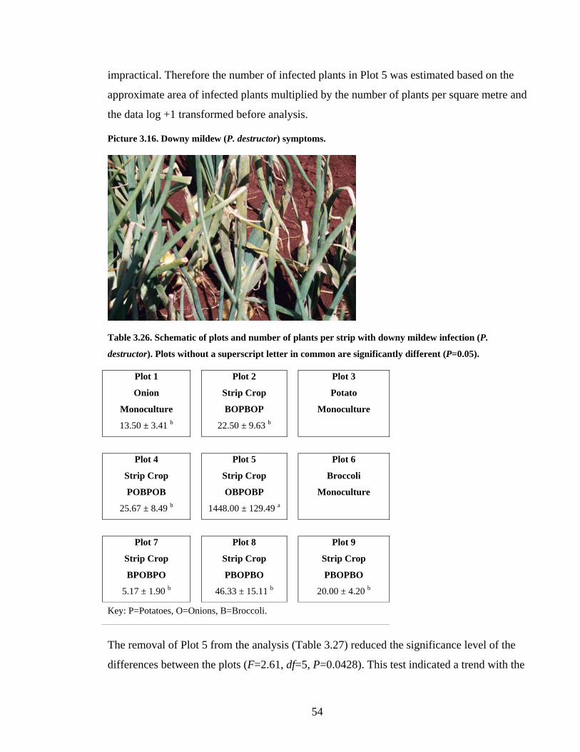
54
impractical. Therefore the number of infected plants in Plot 5 was estimated based on the
approximate area of infected plants multiplied by the number of plants per square metre and
the data log +1 transformed before analysis.
Picture 3.16. Downy mildew (P. destructor) symptoms.
Table 3.26. Schematic of plots and number of plants per strip with downy mildew infection (P.
destructor). Plots without a superscript letter in common are significantly different (P=0.05).
Plot 1
Onion
Monoculture
13.50 ± 3.41 b
Plot 2
Strip Crop
BOPBOP
22.50 ± 9.63 b
Plot 3
Potato
Monoculture
Plot 4
Strip Crop
POBPOB
25.67 ± 8.49 b
Plot 5
Strip Crop
OBPOBP
1448.00 ± 129.49 a
Plot 6
Broccoli
Monoculture
Plot 7
Strip Crop
BPOBPO
5.17 ± 1.90 b
Plot 8
Strip Crop
PBOPBO
46.33 ± 15.11 b
Plot 9
Strip Crop
PBOPBO
20.00 ± 4.20 b
Key: P=Potatoes, O=Onions, B=Broccoli.
The removal of Plot 5 from the analysis (Table 3.27) reduced the significance level of the
differences between the plots (F=2.61, df=5, P=0.0428). This test indicated a trend with the

55
nearest plots to the main site of infection (Plots 2, 4 and 8) having higher infection rates
than the plots furthest away from the outbreak (Plots 1, 7 and 9).
Table 3.27. Mean downy mildew (P. destructor) incidence with Plot 5 removed. Plots without a
superscript letter in common are significantly different (P=0.05).
Plot Strip Arrangement Number (n) Mean number of infected plants
1 Monoculture 18 13.50 ± 3.41 b
2 BOPBOP 6 22.50 ± 9.63 b
4 POBPOB 6 25.67 ± 8.49 ab
7 BPOBPO 6 5.17 ± 1.90 b
8 PBOPBO 6 46.33 ± 15.11 a
9 OPBOPB 6 20.00 ± 4.20 b
Key: P=Potatoes, O=Onions, B=Broccoli.
The high number of infected plants in Plot 5 made the analysis of the effect of neighbouring
plant configurations (Table 3.28) (F=0.28, df=4, P=0.8865) and the planned pairwise
contrasts insignificant (Table 3.29).
Table 3.28. Mean downy mildew (P. destructor) incidence compared to neighbouring plant
configurations.
Neighbouring plant Number
(n)
Non transformed data
± SE
Transformed data
(Log +1) ± SE
Onion monoculture 16 14.875 ± 3.688 2.093 ± 0.351
Broccoli edges 10 338.200 ± 207.146 3.746 ± 0.690
Potato edges 10 192.100 ± 167.826 3.173 ± 0.607
Plot edges 6 148.333 ± 136.035 2.791 ± 0.929
Middle strip rows 12 268.167 ± 166.480 3.312 ± 0.626
Table 3.29. Planned pairwise contrasts of downy mildew (P. destructor) incidence and various
neighbouring plant configurations and onion monoculture (df=1).
Contrast F P
Broccoli edge vs. Onion monoculture 0.88 0.3546
Potato edge vs. Onion monoculture 0.82 0.3718
Plot edges vs. Onion monoculture 0.49 0.4887
Strip middle rows vs. Onion monoculture 1.10 0.3008
Monoculture vs. Strip Cropping 0.99 0.3251
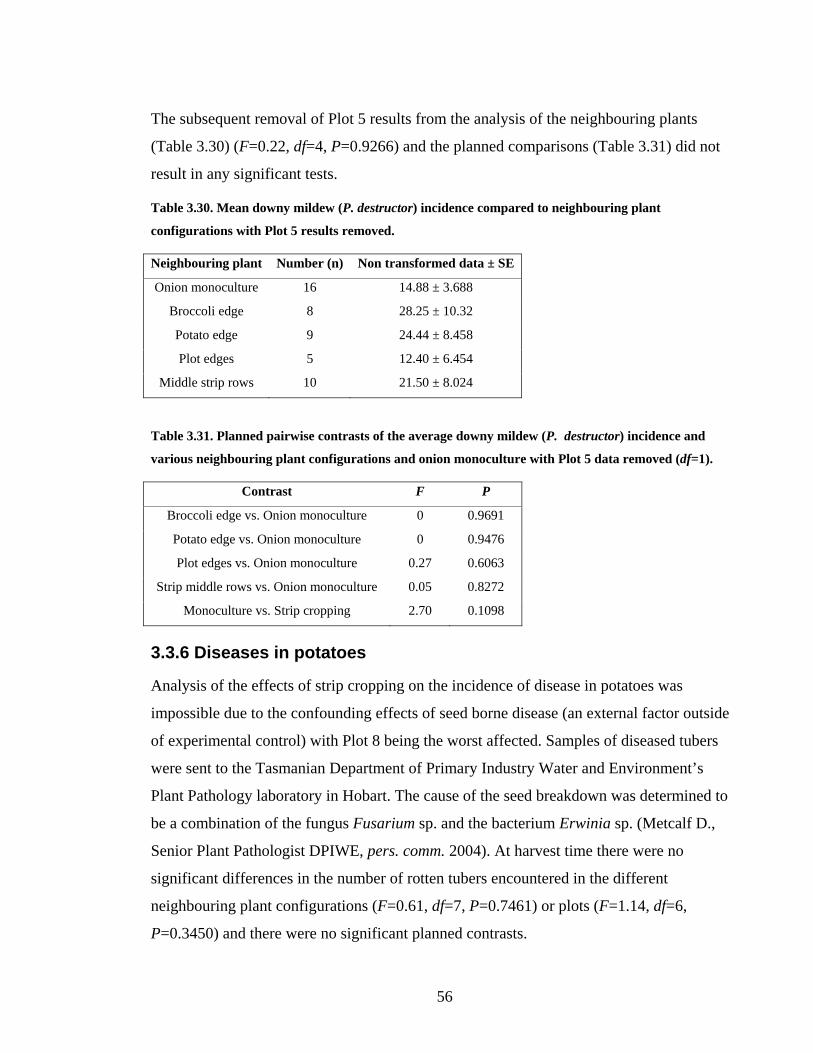
56
The subsequent removal of Plot 5 results from the analysis of the neighbouring plants
(Table 3.30) (F=0.22, df=4, P=0.9266) and the planned comparisons (Table 3.31) did not
result in any significant tests.
Table 3.30. Mean downy mildew (P. destructor) incidence compared to neighbouring plant
configurations with Plot 5 results removed.
Neighbouring plant Number (n) Non transformed data ± SE
Onion monoculture 16 14.88 ± 3.688
Broccoli edge 8 28.25 ± 10.32
Potato edge 9 24.44 ± 8.458
Plot edges 5 12.40 ± 6.454
Middle strip rows 10 21.50 ± 8.024
Table 3.31. Planned pairwise contrasts of the average downy mildew (P. destructor) incidence and
various neighbouring plant configurations and onion monoculture with Plot 5 data removed (df=1).
Contrast F P
Broccoli edge vs. Onion monoculture 0 0.9691
Potato edge vs. Onion monoculture 0 0.9476
Plot edges vs. Onion monoculture 0.27 0.6063
Strip middle rows vs. Onion monoculture 0.05 0.8272
Monoculture vs. Strip cropping 2.70 0.1098
3.3.6 Diseases in potatoes
Analysis of the effects of strip cropping on the incidence of disease in potatoes was
impossible due to the confounding effects of seed borne disease (an external factor outside
of experimental control) with Plot 8 being the worst affected. Samples of diseased tubers
were sent to the Tasmanian Department of Primary Industry Water and Environment’s
Plant Pathology laboratory in Hobart. The cause of the seed breakdown was determined to
be a combination of the fungus Fusarium sp. and the bacterium Erwinia sp. (Metcalf D.,
Senior Plant Pathologist DPIWE, pers. comm. 2004). At harvest time there were no
significant differences in the number of rotten tubers encountered in the different
neighbouring plant configurations (F=0.61, df=7, P=0.7461) or plots (F=1.14, df=6,
P=0.3450) and there were no significant planned contrasts.

57
3.3.7 Diseases in broccoli
The only disease encountered in the broccoli crops was white blister rust (Albugo candida).
This is a relatively new disease of Brassica crops in Australia and was first located in the
outer plot edge of Plot 7 on 10 December 2003 during the regular monitoring of the
experimental area. Spread of the disease meant that at the time of the first harvest on the 9
January 2004, the disease was present in the entire experimental area. The main
consequence of this disease is the rejection of broccoli heads due to visual presence of the
rust fungus, which looks like white paint flecks (Picture 3.15). Therefore, the presence of
the disease was only recorded after harvest as the percentage of the harvested heads
rejected. The analysis of the broccoli harvest rejection rates due to the white blister rust
indicated that there were significant differences between the neighbouring plant
configurations (F=3.70, df=6, P=0.0015) (Table 3.32).
Table 3.32. Percentage of the broccoli harvest rejected due to white blister rust (A. candida) compared
to neighbouring plant configurations. Neighbouring plants without a superscript letter in common are
significantly different (P=0.05).
Neighbouring plant Number (n) Percentage of
broccoli rejected ± SE
Broccoli monoculture 32 18.39 ± 1.559 c
Outer potato edges 10 18.11 ± 4.477 c
Inner potato edges 10 21.29 ± 4.598 bc
Outer onion edges 10 34.41 ± 4.198 a
Inner onion edges 10 33.37 ± 3.457 a
Outer plot edges 6 33.28 ± 7.674 a
Inner plot edges 6 28.70 ± 6.379 ab
Middle strip rows 24 30.95 ± 2.308 a
Further analysis of the results over the four broccoli cuts revealed that most of the
differences in the harvest rejection rates occurred in the final two cuts (Table 3.33).
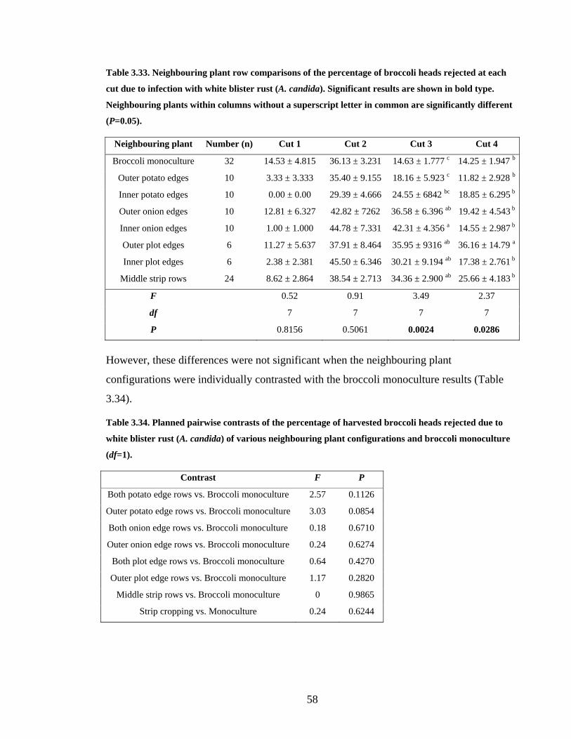
58
Table 3.33. Neighbouring plant row comparisons of the percentage of broccoli heads rejected at each
cut due to infection with white blister rust (A. candida). Significant results are shown in bold type.
Neighbouring plants within columns without a superscript letter in common are significantly different
(P=0.05).
Neighbouring plant Number (n) Cut 1 Cut 2 Cut 3 Cut 4
Broccoli monoculture 32 14.53 ± 4.815 36.13 ± 3.231 14.63 ± 1.777 c 14.25 ± 1.947 b
Outer potato edges 10 3.33 ± 3.333 35.40 ± 9.155 18.16 ± 5.923 c 11.82 ± 2.928 b
Inner potato edges 10 0.00 ± 0.00 29.39 ± 4.666 24.55 ± 6842 bc 18.85 ± 6.295 b
Outer onion edges 10 12.81 ± 6.327 42.82 ± 7262 36.58 ± 6.396 ab 19.42 ± 4.543 b
Inner onion edges 10 1.00 ± 1.000 44.78 ± 7.331 42.31 ± 4.356 a 14.55 ± 2.987 b
Outer plot edges 6 11.27 ± 5.637 37.91 ± 8.464 35.95 ± 9316 ab 36.16 ± 14.79 a
Inner plot edges 6 2.38 ± 2.381 45.50 ± 6.346 30.21 ± 9.194 ab 17.38 ± 2.761 b
Middle strip rows 24 8.62 ± 2.864 38.54 ± 2.713 34.36 ± 2.900 ab 25.66 ± 4.183 b
F 0.52 0.91 3.49 2.37
df 7 7 7 7
P 0.8156 0.5061 0.0024 0.0286
However, these differences were not significant when the neighbouring plant
configurations were individually contrasted with the broccoli monoculture results (Table
3.34).
Table 3.34. Planned pairwise contrasts of the percentage of harvested broccoli heads rejected due to
white blister rust (A. candida) of various neighbouring plant configurations and broccoli monoculture
(df=1).
Contrast F P
Both potato edge rows vs. Broccoli monoculture 2.57 0.1126
Outer potato edge rows vs. Broccoli monoculture 3.03 0.0854
Both onion edge rows vs. Broccoli monoculture 0.18 0.6710
Outer onion edge rows vs. Broccoli monoculture 0.24 0.6274
Both plot edge rows vs. Broccoli monoculture 0.64 0.4270
Outer plot edge rows vs. Broccoli monoculture 1.17 0.2820
Middle strip rows vs. Broccoli monoculture 0 0.9865
Strip cropping vs. Monoculture 0.24 0.6244

59
Analysis of the contrasts at each cut also did not indicate any significant differences (Table
3.35).
Table 3.35. Planned pairwise contrasts of the percentage of broccoli heads rejected at each cut due to
white blister rust (A. candida) of various neighbouring plant configurations and broccoli monoculture
(df=1).
Cut 1 Cut 2 Cut 3 Cut 4 Contrast
F P F P F P F P
Both potato edge rows vs.
Broccoli monoculture 1.46 0.2306 0.44 0.5093 2.34 0.1299 0.85 0.3587
Outer potato edge row vs.
Broccoli monoculture 1.12 0.2937 0.08 0.7807 3.21 0.0765 1.35 0.2483
Both onion edge rows vs.
Broccoli monoculture 0.94 0.3361 0.06 0.8024 0.22 0.6416 0.61 0.4362
Outer onion edge row vs.
Broccoli monoculture 0.34 0.5603 0.03 0.8521 0.03 0.8643 0.31 0.5786
Both plot edge rows vs.
Broccoli monoculture 0.77 0.3823 0.34 0.5609 0.34 0.5639 0.59 0.4461
Outer plot edge rows vs.
Broccoli monoculture 0.25 0.6183 0.64 0.4255 0.76 0.3867 3.58 0.0618
Middle strip rows vs.
Broccoli monoculture 0.64 0.4259 0.17 0.6808 0.03 0.8725 0 0.9445
Strip cropping vs.
Monoculture 1.14 0.2895 0.07 0.7991 0.22 0.6372 0.52 0.4726
White blister rust was present in all of the experimental broccoli plots, however the disease
was concentrated in Plot 7 where it was first located (Table 3.36). This is illustrated by a
significant difference between the plots (F=5.66, df=6, P<0.0001) with Plot 7 having the
highest percentage of harvest rejection.
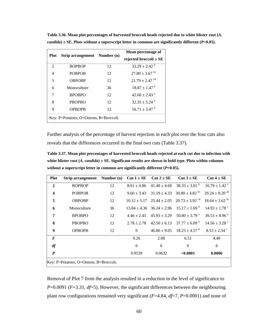
60
Table 3.36. Mean plot percentages of harvested broccoli heads rejected due to white blister rust (A.
candida) ± SE. Plots without a superscript letter in common are significantly different (P=0.05).
Plot Strip arrangement Number (n) Mean percentage of
rejected broccoli ± SE
2 BOPBOP 12 33.29 ± 2.42 b
4 POBPOB 12 27.89 ± 3.67 bc
5 OBPOBP 12 21.79 ± 2.47 cd
6 Monoculture 36 18.87 ± 1.47 d
7 BPOBPO 12 42.60 ± 2.43 a
8 PBOPBO 12 32.35 ± 5.24 b
9 OPBOPB 12 16.71 ± 3.47 d
Key: P=Potatoes, O=Onions, B=Broccoli.
Further analysis of the percentage of harvest rejection in each plot over the four cuts also
reveals that the differences occurred in the final two cuts (Table 3.37).
Table 3.37. Mean plot percentages of harvested broccoli heads rejected at each cut due to infection with
white blister rust (A. candida) ± SE. Significant results are shown in bold type. Plots within columns
without a superscript letter in common are significantly different (P=0.05).
Plot Strip arrangement Number (n) Cut 1 ± SE Cut 2 ± SE Cut 3 ± SE Cut 4 ± SE
2 BOPBOP 12 8.61 ± 4.86 41.48 ± 4.68 38.33 ± 3.81 b 16.79 ± 1.42 c
4 POBPOB 12 9.60 ± 3.43 31.19 ± 4.33 30.80 ± 4.82 bc 29.24 ± 8.20 ab
5 OBPOBP 12 10.12 ± 5.17 25.44 ± 2.05 20.73 ± 3.92 cd 18.64 ± 3.62 bc
6 Monoculture 36 13.84 ± 4.36 36.24 ± 2.96 15.17 ± 1.69 d 14.93 ± 1.78 c
7 BPOBPO 12 4.46 ± 2.45 45.93 ± 3.29 50.80 ± 3.79 a 39.53 ± 8.96 a
8 PBOPBO 12 2.78 ± 2.78 42.50 ± 6.13 37.77 ± 6.09 b 14.56 ± 3.28 c
9 OPBOPB 12 0 46.86 ± 9.05 18.23 ± 4.57 d 8.53 ± 2.34 c
F 0.26 2.08 6.51 4.40
df 6 6 6 6
P 0.9539 0.0632 <0.0001 0.0006
Key: P=Potatoes, O=Onions, B=Broccoli.
Removal of Plot 7 from the analysis resulted in a reduction in the level of significance to
P=0.0091 (F=3.31, df=5). However, the significant differences between the neighbouring
plant row configurations remained very significant (F=4.84, df=7, P=0.0001) and none of
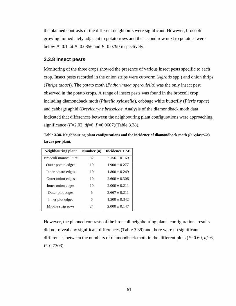
61
the planned contrasts of the different neighbours were significant. However, broccoli
growing immediately adjacent to potato rows and the second row next to potatoes were
below P=0.1, at P=0.0856 and P=0.0790 respectively.
3.3.8 Insect pests
Monitoring of the three crops showed the presence of various insect pests specific to each
crop. Insect pests recorded in the onion strips were cutworm (Agrotis spp.) and onion thrips
(Thrips tabaci). The potato moth (Phthorimaea operculella) was the only insect pest
observed in the potato crops. A range of insect pests was found in the broccoli crop
including diamondback moth (Plutella xylostella), cabbage white butterfly (Pieris rapae)
and cabbage aphid (Brevicoryne brassicae. Analysis of the diamondback moth data
indicated that differences between the neighbouring plant configurations were approaching
significance (F=2.02, df=6, P=0.0607)(Table 3.38).
Table 3.38. Neighbouring plant configurations and the incidence of diamondback moth (P. xylostella)
larvae per plant.
Neighbouring plant Number (n) Incidence ± SE
Broccoli monoculture 32 2.156 ± 0.169
Outer potato edges 10 1.900 ± 0.277
Inner potato edges 10 1.800 ± 0.249
Outer onion edges 10 2.600 ± 0.306
Inner onion edges 10 2.000 ± 0.211
Outer plot edges 6 2.667 ± 0.211
Inner plot edges 6 1.500 ± 0.342
Middle strip rows 24 2.000 ± 0.147
However, the planned contrasts of the broccoli neighbouring plants configurations results
did not reveal any significant differences (Table 3.39) and there were no significant
differences between the numbers of diamondback moth in the different plots (F=0.60, df=6,
P=0.7303).

62
Table 3.39. Planned pairwise contrasts of the incidence of diamondback moth (P. xylostella) in
neighbouring plant row configurations and the broccoli monoculture (df=1).
Contrast F P
Both potato edge rows vs. Broccoli monoculture 2.79 0.0984
Outer potato edge row vs. Broccoli monoculture 2.27 0.1351
Both Onion edge rows vs. Broccoli monoculture 0.65 0.4222
Outer Onion edge row vs. Broccoli monoculture 0.08 0.7844
Both plot edge rows vs. Broccoli monoculture 1.55 0.2168
Outer plot edge rows vs. Broccoli monoculture 0 0.9917
Middle strip rows vs. Broccoli monoculture 1.96 0.1653
Strip cropping vs. Monoculture 1.73 0.1924
While the distribution of the remaining insects was not measured due to time constraints
and low numbers, there also appeared to be no differences across the neighbouring plant
configurations and there were no apparent adverse or beneficial effects due to the close
proximity of different crops.
3.4 Discussion
3.4.1 Crop yields
When the yield rankings and the LSD groupings of the three crops were combined it can be
seen that overall Plots 7, 8 and 9 were the lowest yielding plots (Table 3.40). The main
explanation for these differences was the non-uniform distribution of water attributed to the
use of a travelling irrigator and the prevalence for strong westerly winds that resulted in
lower application rates in upwind plots (7,8 and 9) and higher application rates in down
wind plots (4, 5 and 6). Plot 7 was slightly lower in elevation than other plots and might
have been partially compensated for the lack of direct irrigation by runoff from the other
plots.
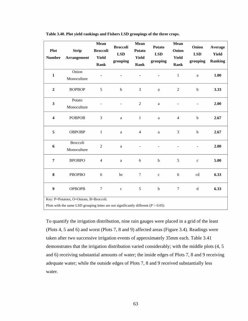
63
Table 3.40. Plot yield rankings and Fishers LSD groupings of the three crops.
Plot
Number
Strip
Arrangement
Mean
Broccoli
Yield
Rank
Broccoli
LSD
grouping
Mean
Potato
Yield
Rank
Potato
LSD
grouping
Mean
Onion
Yield
Rank
Onion
LSD
grouping
Average
Yield
Ranking
1 Onion
Monoculture - - - - 1 a 1.00
2 BOPBOP 5 b 3 a 2 b 3.33
3 Potato
Monoculture - - 2 a - - 2.00
4 POBPOB 3 a 1 a 4 b 2.67
5 OBPOBP 1 a 4 a 3 b 2.67
6 Broccoli
Monoculture 2 a - - - - 2.00
7 BPOBPO 4 a 6 b 5 c 5.00
8 PBOPBO 6 bc 7 c 6 cd 6.33
9 OPBOPB 7 c 5 b 7 d 6.33
Key: P=Potatoes, O=Onions, B=Broccoli.
Plots with the same LSD grouping letter are not significantly different (P > 0.05)
To quantify the irrigation distribution, nine rain gauges were placed in a grid of the least
(Plots 4, 5 and 6) and worst (Plots 7, 8 and 9) affected areas (Figure 3.4). Readings were
taken after two successive irrigation events of approximately 35mm each. Table 3.41
demonstrates that the irrigation distribution varied considerably; with the middle plots (4, 5
and 6) receiving substantial amounts of water; the inside edges of Plots 7, 8 and 9 receiving
adequate water; while the outside edges of Plots 7, 8 and 9 received substantially less
water.
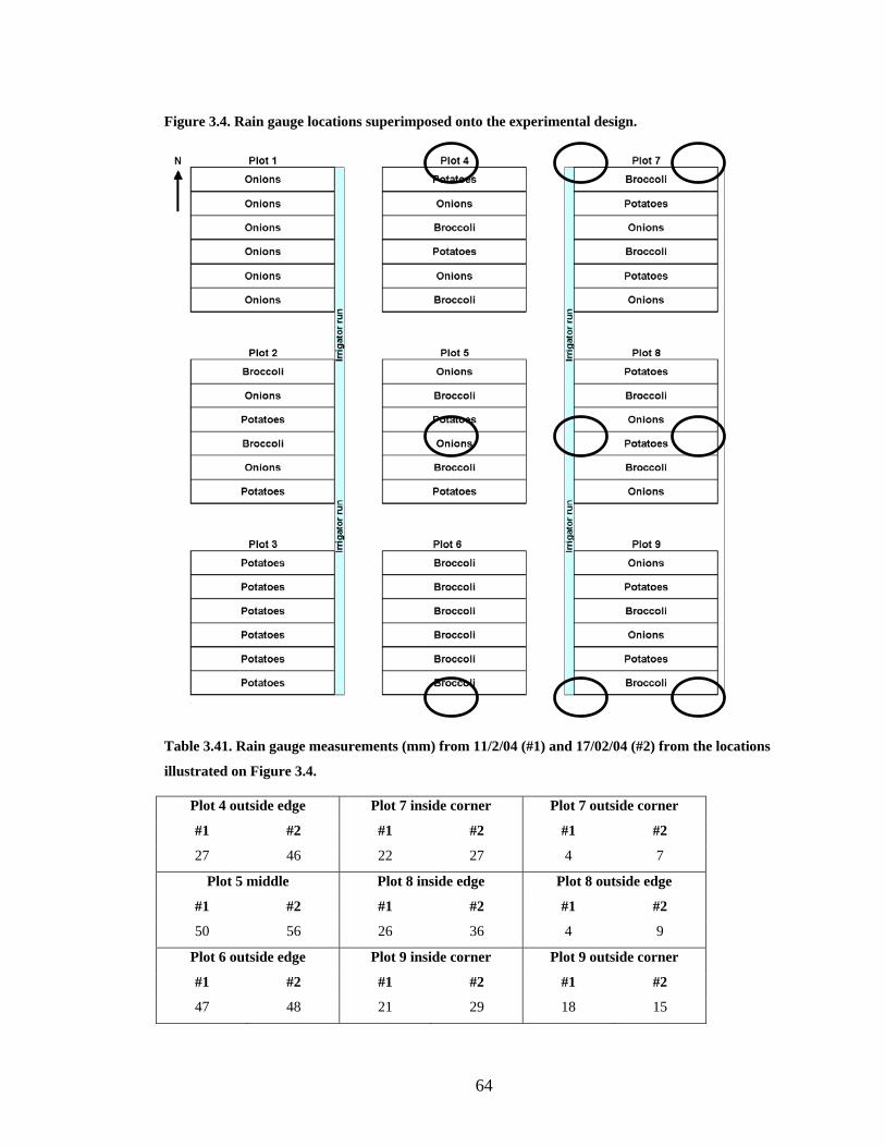
64
Figure 3.4. Rain gauge locations superimposed onto the experimental design.
Table 3.41. Rain gauge measurements (mm) from 11/2/04 (#1) and 17/02/04 (#2) from the locations
illustrated on Figure 3.4.
Plot 4 outside edge Plot 7 inside corner Plot 7 outside corner
#1 #2 #1 #2 #1 #2
27 46 22 27 4 7
Plot 5 middle Plot 8 inside edge Plot 8 outside edge
#1 #2 #1 #2 #1 #2
50 56 26 36 4 9
Plot 6 outside edge Plot 9 inside corner Plot 9 outside corner
#1 #2 #1 #2 #1 #2
47 48 21 29 18 15
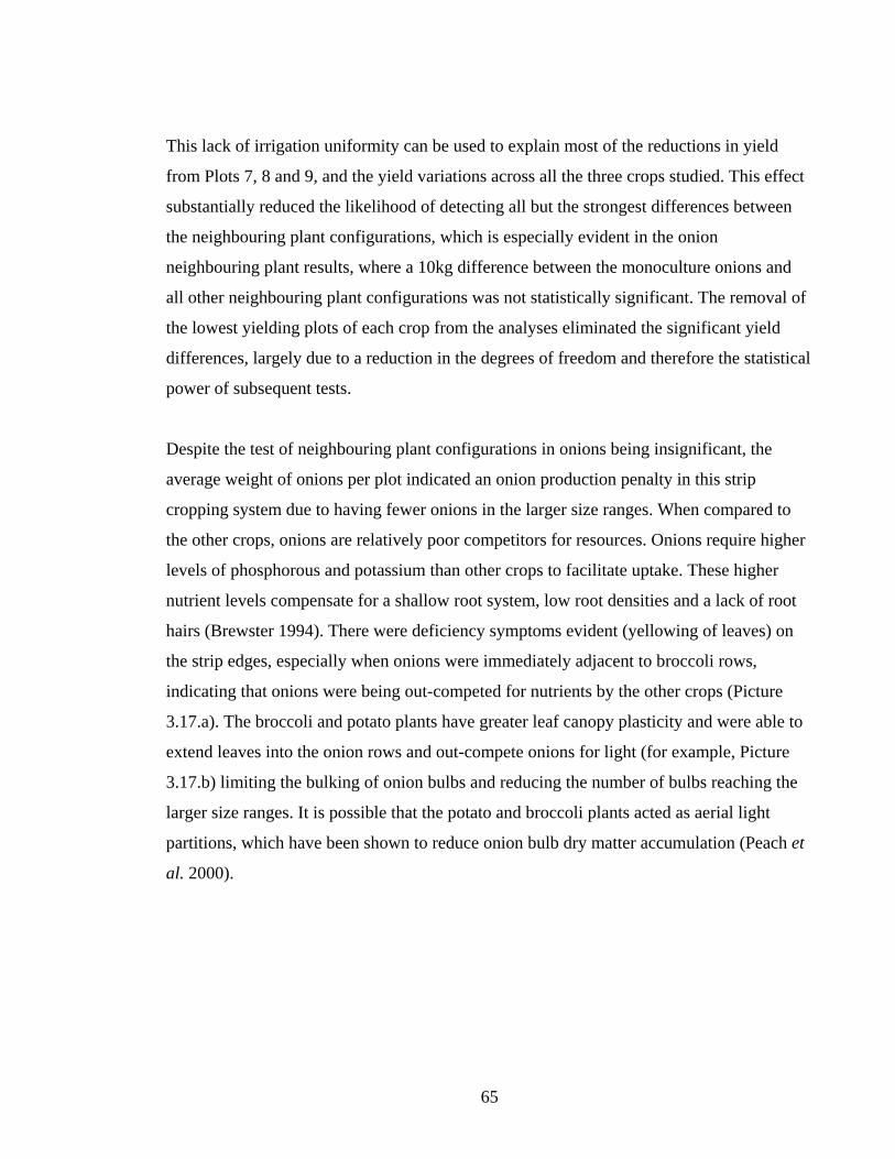
65
This lack of irrigation uniformity can be used to explain most of the reductions in yield
from Plots 7, 8 and 9, and the yield variations across all the three crops studied. This effect
substantially reduced the likelihood of detecting all but the strongest differences between
the neighbouring plant configurations, which is especially evident in the onion
neighbouring plant results, where a 10kg difference between the monoculture onions and
all other neighbouring plant configurations was not statistically significant. The removal of
the lowest yielding plots of each crop from the analyses eliminated the significant yield
differences, largely due to a reduction in the degrees of freedom and therefore the statistical
power of subsequent tests.
Despite the test of neighbouring plant configurations in onions being insignificant, the
average weight of onions per plot indicated an onion production penalty in this strip
cropping system due to having fewer onions in the larger size ranges. When compared to
the other crops, onions are relatively poor competitors for resources. Onions require higher
levels of phosphorous and potassium than other crops to facilitate uptake. These higher
nutrient levels compensate for a shallow root system, low root densities and a lack of root
hairs (Brewster 1994). There were deficiency symptoms evident (yellowing of leaves) on
the strip edges, especially when onions were immediately adjacent to broccoli rows,
indicating that onions were being out-competed for nutrients by the other crops (Picture
3.17.a). The broccoli and potato plants have greater leaf canopy plasticity and were able to
extend leaves into the onion rows and out-compete onions for light (for example, Picture
3.17.b) limiting the bulking of onion bulbs and reducing the number of bulbs reaching the
larger size ranges. It is possible that the potato and broccoli plants acted as aerial light
partitions, which have been shown to reduce onion bulb dry matter accumulation (Peach et
al. 2000).
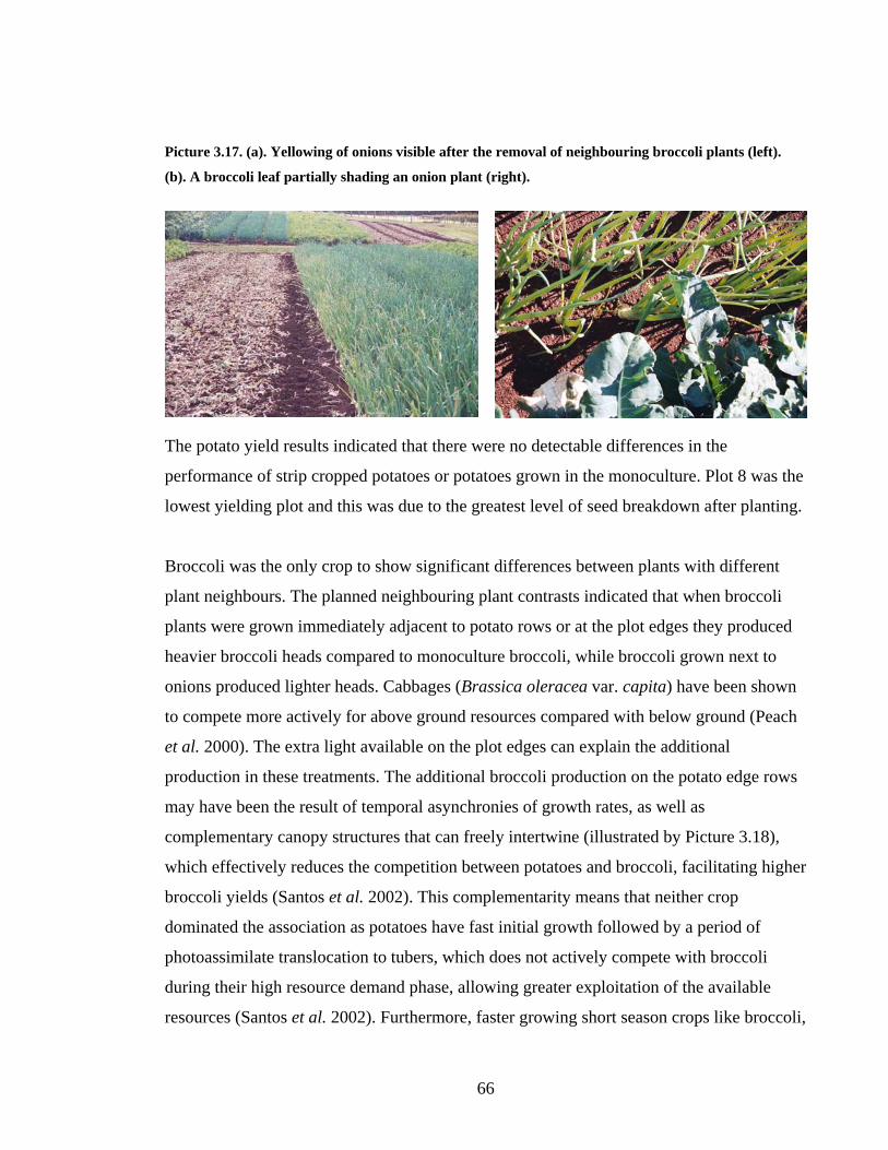
66
Picture 3.17. (a). Yellowing of onions visible after the removal of neighbouring broccoli plants (left).
(b). A broccoli leaf partially shading an onion plant (right).
The potato yield results indicated that there were no detectable differences in the
performance of strip cropped potatoes or potatoes grown in the monoculture. Plot 8 was the
lowest yielding plot and this was due to the greatest level of seed breakdown after planting.
Broccoli was the only crop to show significant differences between plants with different
plant neighbours. The planned neighbouring plant contrasts indicated that when broccoli
plants were grown immediately adjacent to potato rows or at the plot edges they produced
heavier broccoli heads compared to monoculture broccoli, while broccoli grown next to
onions produced lighter heads. Cabbages (Brassica oleracea var. capita) have been shown
to compete more actively for above ground resources compared with below ground (Peach
et al. 2000). The extra light available on the plot edges can explain the additional
production in these treatments. The additional broccoli production on the potato edge rows
may have been the result of temporal asynchronies of growth rates, as well as
complementary canopy structures that can freely intertwine (illustrated by Picture 3.18),
which effectively reduces the competition between potatoes and broccoli, facilitating higher
broccoli yields (Santos et al. 2002). This complementarity means that neither crop
dominated the association as potatoes have fast initial growth followed by a period of
photoassimilate translocation to tubers, which does not actively compete with broccoli
during their high resource demand phase, allowing greater exploitation of the available
resources (Santos et al. 2002). Furthermore, faster growing short season crops like broccoli,

67
generally suffer less from competition for light (Keating and Carberry 1993) reducing the
likelihood of higher yields on the strip edges. The lower yields of broccoli next to onions
was most likely due to the close proximity of the onion rows (40cm from the broccoli
plants as opposed to 80cm in the other treatments) and their high planting density, which
increased competition for resources.
Picture 3.18. Complementarity of potato and broccoli leaf canopies on a strip edge with potatoes on the
left and broccoli on the right.
3.4.2 Plant diseases
The analysis of the plant disease data was inhibited by the rapid onset of diseases, largely
as a result of a planned absence of chemical disease protectants and an abnormal weather
event in January. The weather event came in the form of a massive downpour of 95 mm on
28 January, followed by falls of 45mm and 16mm over the next two days. The initial
rainfall on the 28 January was substantially higher than the previous single day January
rainfall total since records began in 1889, with the next highest totals being 62mm on the
25/1/1991 and 50mm on the 20/1/1942. The 95mm helped the total rainfall in January to
161mm, which was also an historical record. Temperatures of between 20-24oC for the

68
following week created a situation where fungal diseases rapidly spread in the onions and
potatoes (broccoli had already been harvested).
While the rainfall event was the catalyst for the disease outbreaks, excess irrigation applied
to the middle plots possibly contributed to the outbreak of downy mildew in the onions of
Plot 5, by allowing the establishment of low levels of disease before January 28, which then
rapidly multiplied in these ideal conditions. However, there was no evidence of differences
in potato disease infection rates across the different neighbouring plant configurations due
to the prevalence of seed borne diseases confounding the disease data.
Analysis of the data of the harvest rejection of broccoli heads due to white blister rust
indicated that plot edges, onion edges and the middle strip rows had higher infection rates.
This suggests that the disease was spread more easily to these zones. However, contrasting
the effect of neighbouring plant rows on harvest rejection rates did not reveal any
statistically significant results. Plot 7 was where the disease was first located and had
significantly higher harvest rejection rates than the remaining plots. The removal of Plot 7
from the analysis did not result in any significant interactions or contrasts, but it did slightly
increase the probability of a significant interaction for broccoli growing immediately
adjacent to potatoes and the second row next to potatoes to below the P=0.1 level to
P=0.0856 and P=0.0790 respectively.
3.4.3 Plutella xylostella (diamondback moth) distribution in broccoli
The analysis of the influence of the neighbouring plant interactions on the number of
diamondback moths (P. xylostella) was approaching significance (P=0.0607), which can be
explained by the low numbers of diamondback moths in the two rows adjacent to potato
plants and the inner plot edge row, and the high numbers in the outer plot edge rows. The
only contrast that was below P=0.1 was the contrast of both potato edge rows and the
monoculture broccoli at P=0.0984. These two pieces of data, although not statistically
significant, indicate that the effects of strip cropping broccoli and potatoes on the presence
of diamondback moths might be worth further investigation.

69
3.5 Implications
Out of all the statistical tests performed there were very few significant results, all of which
occurred between broccoli rows adjacent to potato rows. Despite the absence of a
significant impact of strip cropping on potatoes, there is enough data to support further
investigation of the interaction of broccoli and potatoes. The poor performance of onions in
strip cropping and their negative impact on broccoli production, indicates that further
experiments with onions are not warranted. Furthermore, the idea that volatiles produced by
crops like onions have the potential to inhibit herbivorous insects (Uvah and Coaker 1984)
has been recently refuted by Finch et al. (2003), bringing into question one of the major
reasons for including onions in the experiment.
There is the possibility of substituting onions with another crop in the design. However, the
study of two crops instead of three would reduce the management burden of subsequent
trials allowing greater replication, more frequent sampling and theoretically a greater
chance of revealing significant interactions. The results also indicate that any interactions
are likely to occur at row edges between the crops and any interactions are unlikely to
penetrate into any of the middle rows of the five-metre per strip design. Therefore there is
no benefit to be derived in these vegetable crops from having more than two 1.65m strips,
with the greatest chance of positive interactions coming from replications of single 1.65m
strips where each row shares an edge row with another crop. Narrowing the experimental
strip width would also allow greater replication in any subsequent designs using less
experimental area, further reducing the management burden. A smaller experimental area
would also facilitate the use of more accurate irrigation equipment reducing the chance of
yield gradients due to lack of irrigation uniformity. Furthermore, if only broccoli and
potatoes are used in further experiments, all the chemical weed control of the potato crop
could be performed before the broccoli is transplanted, eliminating the need for specially
designed spray equipment. However, further reducing each crop width to individual rows to
make the system a true polyculture (both potatoes and broccoli in each 1.65m row) is
impractical as the crops could not be planted and harvested using existing equipment and
would unnecessarily complicate the cropping system.
70
There was little evidence of beneficial interactions reducing plant diseases or insect pests in
the different crop configurations and no evidence of cross contamination. Downy mildew
and white blister rust were not evenly distributed across the plots, which might indicate that
disease spread from an initial source of infection was slowed by strip crops and the plot
arrangements. The alternating pattern of the vegetable strips and plots might have acted as
physical barriers between susceptible plants (Altieri and Liebman 1986; Potts 1990; Finckh
and Mundt 1992) as the spread of many diseases is related to the density of susceptible
plants per unit area (Potts 1990). However, the assessment of plant diseases in these crops
and in this system was problematic due to the rapid onset of diseases and the ubiquitous
nature of the pathogens. In general, the effects of diversification on diseases in plant
diversity experiments are hard to predict due to complicated interactions between pathogen
dispersal processes, infection efficiency and altered microclimates (Matson et al. 1997) and
therefore are not a major focus in further experiments.

71
Chapter 4 The impacts of a rye cover crop and strip crops on insect pests of broccoli
4.1 Introduction
To investigate research questions identified in Chapter 2 and to build on the preliminary
investigations discussed in Chapter 3, an additional layer of diversity, in the form of a cover
crop, was added to field experiments conducted in the summers of 2004/2005 and
2005/2006. The results from the insect monitoring activities are discussed in this chapter
and the agronomic results in Chapter 5. Although the agronomic interactions were
important in understanding the differences between conventional practices, strip crops and
cover crops, the insect responses observed in the 04/05 trial were more promising than the
agronomic results. Therefore, a greater emphasis was placed on insect research in the 05/06
experiment.
4.2 Insect pests in Brassica cropping systems
The risk of insect damage and contamination of Brassica vegetable crops results in the
frequent application of insecticides during the cropping season (Baker and Kovaliski 1999).
However, the sole reliance on insecticides is ill advised due to the cost, consumer concerns
and quality assurance issues in relation to chemical residues and the potential for the
development of insecticide resistance (Hamilton et al. 2004). Plutella xylostella (Linnaeus)
(Lepidoptera: Plutellidae) is the most destructive pest of Brassica crops throughout the
world (Talekar and Shelton 1993) and is also the major pest in Australia (Endersby et al.
2006) where it is commonly known as the diamondback moth. This insect is of particular
concern to farmers due to the development of multiple chemical resistance, which has led
to insecticide control failures in Australia (Baker and Kovaliski 1999) and around the world
(Zhao et al. 2002). This has led to the development of integrated pest management (IPM)
and chemical rotation (resistance management) strategies in Australia (Baker 2004), the
success of which is largely reliant on grower adherence to the guidelines. Various parasitic
wasps have also been introduced to Australia to control P. xylostella (Furlong et al. 2004),
but these are typically not effective as a stand alone control strategy (Keller and Baker

72
2003; Furlong et al. 2004). In some situations, like Tasmania, these biological control
agents are often overwhelmed by large influxes of pests migrating from other breeding
centres on favourable winds (Hill 1993). These factors suggest that alternative P. xylostella
control strategies should be researched and developed. The use of crop diversification may
be an alternative method of reducing the use of synthetic chemicals in Brassica cropping
systems due to possible interference with host location, host acceptance and oviposition
processes (Chapter 2). Two possible diversification strategies identified were strip cropping
broccoli with potatoes and the use of a cover crop. The effectiveness of these strategies in
reducing P. xylostella numbers in broccoli, when compared to the current practice of
growing broccoli in a monoculture with extensively cultivated (bare) soil, will be the focus
of this chapter. Two other pest species of lessor importance, the cabbage white butterfly
Pieris rapae (L.)(Lepidoptera: Pieridae) and the cabbage aphid Brevicoryne brassicae
(L.)(Homoptera: Aphididae) were also encountered in the broccoli plots and these will also
be discussed.
4.3 Life histories of the major insect pests of Brassicas in
Australia
4.3.1 Plutella xylostella
P. xylostella is a specialist herbivore of wild and cultivated plants of the Brassicaceae
family with a cosmopolitan distribution (that is, the insect is found wherever Brassicas are
cultivated). It is thought that P. xylostella originated in the Mediterranean where Brassica
crops were first domesticated, although there is some evidence that the pest could have
come from Africa (Kfir 1998). It is believed that P. xylostella had arrived in Australia by at
least 1889 (Waterhouse and Sands 2001). The following life history of P. xylostella is
based on the scientific description of this insect by Harcourt (1957).
Minute eggs, approximately 1.2mm in diameter, are typically laid on the leaves of the host
plant. Each egg incubates for 4-7 days and then the newly hatched larva bores through the
leaf epidermis and the first of four instars mines the spongy leaf mesophyll tissue from
inside the leaf. The second instar moves to the surface and begins consuming all the leaf
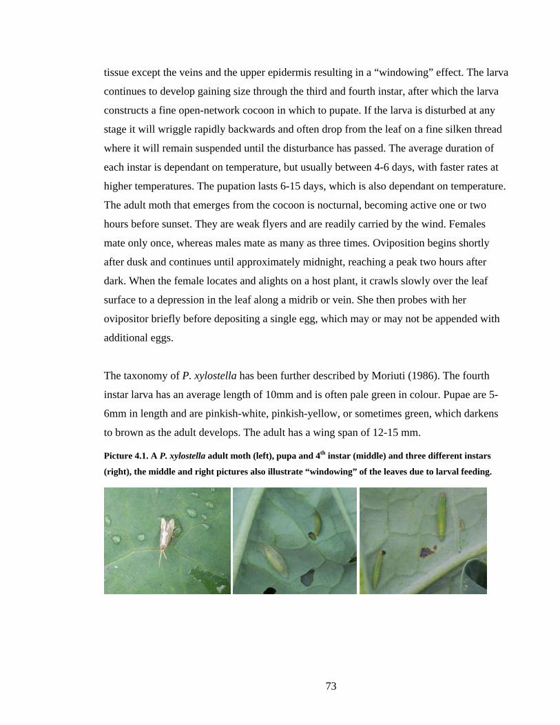
73
tissue except the veins and the upper epidermis resulting in a “windowing” effect. The larva
continues to develop gaining size through the third and fourth instar, after which the larva
constructs a fine open-network cocoon in which to pupate. If the larva is disturbed at any
stage it will wriggle rapidly backwards and often drop from the leaf on a fine silken thread
where it will remain suspended until the disturbance has passed. The average duration of
each instar is dependant on temperature, but usually between 4-6 days, with faster rates at
higher temperatures. The pupation lasts 6-15 days, which is also dependant on temperature.
The adult moth that emerges from the cocoon is nocturnal, becoming active one or two
hours before sunset. They are weak flyers and are readily carried by the wind. Females
mate only once, whereas males mate as many as three times. Oviposition begins shortly
after dusk and continues until approximately midnight, reaching a peak two hours after
dark. When the female locates and alights on a host plant, it crawls slowly over the leaf
surface to a depression in the leaf along a midrib or vein. She then probes with her
ovipositor briefly before depositing a single egg, which may or may not be appended with
additional eggs.
The taxonomy of P. xylostella has been further described by Moriuti (1986). The fourth
instar larva has an average length of 10mm and is often pale green in colour. Pupae are 5-
6mm in length and are pinkish-white, pinkish-yellow, or sometimes green, which darkens
to brown as the adult develops. The adult has a wing span of 12-15 mm.
Picture 4.1. A P. xylostella adult moth (left), pupa and 4th instar (middle) and three different instars
(right), the middle and right pictures also illustrate “windowing” of the leaves due to larval feeding.
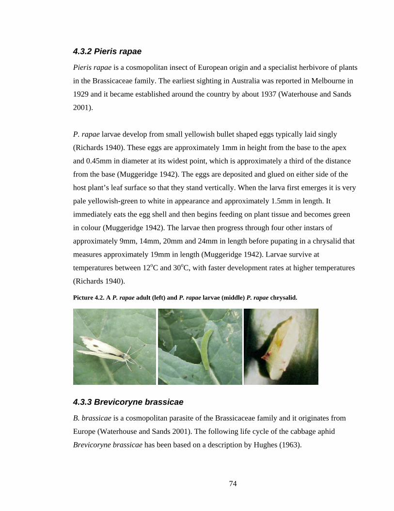
74
4.3.2 Pieris rapae
Pieris rapae is a cosmopolitan insect of European origin and a specialist herbivore of plants
in the Brassicaceae family. The earliest sighting in Australia was reported in Melbourne in
1929 and it became established around the country by about 1937 (Waterhouse and Sands
2001).
P. rapae larvae develop from small yellowish bullet shaped eggs typically laid singly
(Richards 1940). These eggs are approximately 1mm in height from the base to the apex
and 0.45mm in diameter at its widest point, which is approximately a third of the distance
from the base (Muggeridge 1942). The eggs are deposited and glued on either side of the
host plant’s leaf surface so that they stand vertically. When the larva first emerges it is very
pale yellowish-green to white in appearance and approximately 1.5mm in length. It
immediately eats the egg shell and then begins feeding on plant tissue and becomes green
in colour (Muggeridge 1942). The larvae then progress through four other instars of
approximately 9mm, 14mm, 20mm and 24mm in length before pupating in a chrysalid that
measures approximately 19mm in length (Muggeridge 1942). Larvae survive at
temperatures between 12oC and 30oC, with faster development rates at higher temperatures
(Richards 1940).
Picture 4.2. A P. rapae adult (left) and P. rapae larvae (middle) P. rapae chrysalid.
4.3.3 Brevicoryne brassicae
B. brassicae is a cosmopolitan parasite of the Brassicaceae family and it originates from
Europe (Waterhouse and Sands 2001). The following life cycle of the cabbage aphid
Brevicoryne brassicae has been based on a description by Hughes (1963).
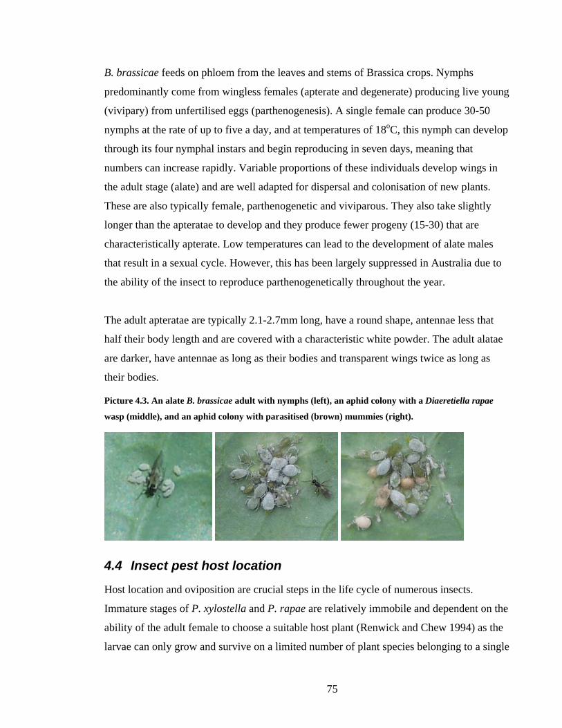
75
B. brassicae feeds on phloem from the leaves and stems of Brassica crops. Nymphs
predominantly come from wingless females (apterate and degenerate) producing live young
(vivipary) from unfertilised eggs (parthenogenesis). A single female can produce 30-50
nymphs at the rate of up to five a day, and at temperatures of 18oC, this nymph can develop
through its four nymphal instars and begin reproducing in seven days, meaning that
numbers can increase rapidly. Variable proportions of these individuals develop wings in
the adult stage (alate) and are well adapted for dispersal and colonisation of new plants.
These are also typically female, parthenogenetic and viviparous. They also take slightly
longer than the apteratae to develop and they produce fewer progeny (15-30) that are
characteristically apterate. Low temperatures can lead to the development of alate males
that result in a sexual cycle. However, this has been largely suppressed in Australia due to
the ability of the insect to reproduce parthenogenetically throughout the year.
The adult apteratae are typically 2.1-2.7mm long, have a round shape, antennae less that
half their body length and are covered with a characteristic white powder. The adult alatae
are darker, have antennae as long as their bodies and transparent wings twice as long as
their bodies.
Picture 4.3. An alate B. brassicae adult with nymphs (left), an aphid colony with a Diaeretiella rapae
wasp (middle), and an aphid colony with parasitised (brown) mummies (right).
4.4 Insect pest host location
Host location and oviposition are crucial steps in the life cycle of numerous insects.
Immature stages of P. xylostella and P. rapae are relatively immobile and dependent on the
ability of the adult female to choose a suitable host plant (Renwick and Chew 1994) as the
larvae can only grow and survive on a limited number of plant species belonging to a single
76
family (Hern et al. 1996). Host location by aphids can be described as a passive process.
The alate adults are relatively poor fliers that are carried by the wind for long distances
(Compton 2002), primarily because they can make no progress against winds of more than
0.6 ms-1 (Hughes 1963). Even for insects like B. brassicae with a narrow host range, their
vision is primarily used to distinguish plants from the sky (Kennedy et al. 1961) and they
have no specific attraction to the host plant over more than a metre distant and will alight
and take off from host and non-host alike resulting in the mortality of upwards of 99% of
individuals (Hughes 1963). It is only a minutely higher probability that they will remain on
a host plant compared to a non-host plant that facilitates colonisation (Hughes 1963). There
is evidence from electro-physiological experiments that B. brassicae respond positively to
host plant volatiles (Nottingham et al. 1991), however these are unlikely to provide
directional information (Finch and Collier 2000) but rather act on host plant acceptance
behaviour after landing has occurred (Compton 2002).
Host location in insects is not necessarily a complicated process. Finch and Collier (2003)
report that phytophagous insects are so successful at locating plants because they have
“kept things simple”. They summarise host location as being made up of three basic steps:-
1. Chemical stimuli (plant odours) indicate when to land.
2. Visual stimuli (colour and contrast) indicate where to land.
3. Touch and taste indicate host suitability and hence whether to stay or fly away.
To reduce colonisation and plant damage, a cropping system has to interfere with one of
these steps. The simplest to alter in a cropping system is the visual stimuli present (where
vision in insects is defined as the ability to perceive spatial patterns [Prokopy and Owens
1983]). This is also arguably the most important as the visual perception of plant colour and
shape are “undoubtedly” the dominant sensory cues for moths and butterflies searching for
host plants (Renwick and Chew 1994). The current practice of “clean” cultivation of crops,
with a zero tolerance of non-crop plants, like weeds and cover crops, ensures that crop
plants are exposed to the maximum pest pressure due to the ease of host location when
there is a high visual contrast between plants and a bare soil background (Finch and Collier
2000). A reduction in the contrast between the soil and the host plants by the use of

77
background vegetation may lead to a reduction in pest pressure. For example, Mangan et al.
(1995) and Masiunas et al. (1997) found fewer insect pests in cabbages grown with cover
crops including cereal rye (Secale cereale) when compared to conventional tillage (a bare
soil background).
Despite decades of field studies there is no reliable, generalised strategy for deploying
diversity into crop fields to manage insect pests, probably due to experimental differences
in insect behaviour; plant physiology and the scale of experiments (Andow 1991; Banks
and Ekbom 1999); inadequate research methods (Smith and McSorley 2000); and the
perpetuation of “myths and untested assumptions” (Finch and Collier 2000) such as volatile
chemicals released from companion crops “masking” the presence of a host plant (Finch et
al. 2003). The spatial arrangement and density of planting may also be a factor because at
higher plant densities, insects locate hosts more readily when uniformly dispersed than
when the plants are clumped (Hern et al. 1996). Furthermore, theoretical mechanisms
accounting for herbivore/plant/predator interactions in plant mixtures have not been
thoroughly evaluated (Hooks and Johnson 2003). These issues have contributed to
ambiguities meaning that few robust generalisations can be made about the effects of
infield plant diversity on insect pest densities.
For crop diversification strategies to be successful, Hooks and Johnson (2003)
recommended that attention should be paid to:
1. Defining ways to suppress Brassica pests without significantly affecting yield.
2. Determining how mixed cropping systems impact population dynamics and host finding
behaviour.
3. Discovering methods to make mixed Brassica systems more economically feasible and
compatible with current conventional farming systems.
4. Determining how mixed cropping systems can be effectively combined with other pest
management practices.
In addition, Schellhorn and Sork (1997) report that the plant mixtures chosen for
diversification strategies need to be of relatively unrelated species, as mixtures of plants
from one family can increase the number of specialist herbivores.

78
Combining a fragmented field, using strip cropping, with a visually diverse background
through the use of a cover crop, could conceivably progress some of these issues and has
the potential to increase the effects of either pest management strategy on host location in
an additive fashion, without affecting yield. Furthermore using tractor width strips
facilitates field management with minimal change to current practices.
4.5 Methodology
The main outcomes of the Preliminary Investigations detailed in Chapter 3 were that onions
were unsuitable for further experimentation in a strip cropping system and that any zone of
interaction was likely to occur on the rows immediately adjacent to an alternative crop. The
removal of onions as a focus crop meant that the size of the experiment area could be
reduced and the replication increased. After incorporating these factors in the design, the
04/05 trial investigated the impact of four cropping systems on the abundance of insect
pests. The cropping systems were based on two factors; the first was either a strip crop
utilising broccoli (Brassica oleracea var. italica) host plants with non-host potatoes
(Solanum tuberosum cv. Russet Burbank) or a broccoli monoculture; the second factor was
using either conventional tillage or a cover crop. The 05/06 trial included another strip
cropping option in the form of dead standing rye strips, and investigated if the effects from
04/05 were caused by interference with oviposition, differential egg survival or changes in
the host quality of the plants in the different treatments.
To avoid repetition, this chapter describes the site and experimental methods that were
common to the experiments in this chapter and Chapter 5. Materials and methods specific
to each chapter are described in the respective chapters.
4.5.1 Choice of the cover crop
One option for increasing diversity in a cropping system is via the addition of a cover crop
or a living mulch (vertical diversity, see Chapter 2). The choice of the cover crop or living
mulch had to take into account the initial goals of this thesis outlined in the Introduction, in

79
that the system with the potential to reduce insect pressure (and potentially reduce chemical
use) should not significantly reduce yield and consequently the income of farmers.
Competition with the harvested crop for light, nutrients and water and the subsequent
reduction in yield is a major problem with living mulches (Root 1973; Horn 1987; Lotz et
al. 1997; Theunissen 1997), which is not effectively suppressed with mowing (Brandsæter
et al. 1998). Furthermore, living mulches are not always effective at reducing weed
pressure (Brandsæter et al. 1998) unless weed pressure is low (Infante and Morse 1996). To
minimise competition for light, nutrients or water, the ground cover crop should be killed
prior to planting the component of the system to be harvested. This “cover crop” should
also be dense, uniformly distributed and managed so that it that covers and shades the soil
in order to suppress weeds (Morse 1998). In transplanted cabbages, a cereal rye (Secale
cereale L.) cover crop killed with glyphosate has been shown to assist in controlling insect
pests while reducing weed populations (Bottenberg et al. 1997). Rye cover crops have also
been shown to reduce crop yields (Mwaja et al. 1996; Bottenberg et al. 1997). However,
the crops in these studies were harvested on a single day, potentially biasing the results as
rye cover crops have been shown to delay harvests by up to three weeks when compared to
crops grown in cultivated soil (Borowy 2004), and would appear to have yielded less. Rye
has the added benefit of being easily killed with a single glyphosate application and/or
rolling (Ashford and Reeves 2003). Furthermore, of 14 cover crops screened by Nelson et
al. (1991), which included grasses, legumes and cereals, rye had the greatest percentage of
ground cover and was the most suppressive of weeds. Masiunas et al. (1997) found that
dead rye was the most promising mulch for cabbage. Similar rye cover crops have also
been trialled previously in Tasmania (Young and Hingston 1993) and on potatoes (Wallace
and Bellinder 1990; Bellinder et al. 1996). For these reasons a cereal rye cover crop was
chosen for inclusion in the following experiments.
4.5.2 Field trial designs
Separate field experiments were conducted in the summers of 2004/2005 and 2005/2006 at
the Forthside Research Station (as per Chapter 3). The 04/05 experiment consisted of three
replications of eight plots in a randomised block. Each plot was 10m x 10m with a 5m

80
separation between plots with bare soil on the sides and grass at each end (Figure 4.1). The
first factor of the experimental design was a continuation of the Preliminary Investigations
of 03/04 (Chapter 3), with either broccoli (Brassica oleracea var. italica cv. Green Belt)
strip cropped with potatoes (Solanum tuberosum cv. Russet Burbank), or broccoli grown in
a monoculture. The second factor constituted the additional layer of diversity, with broccoli
either transplanted into a chemically killed and mechanically rolled rye (Secale cereale)
cover crop or into conventionally tilled soil. To maintain balanced numbers of broccoli
plants in each treatment, there were two strip cropping plots to each monoculture plot per
replication (Picture 4.4). Ignoring the potato monocultures, the treatments were grouped as
follows:
1. Broccoli monoculture planted in a rye cover crop (Cover crop/Monoculture).
2. Broccoli and potato strip crop planted into a rye cover crop (Cover crop/Potato
strips) in two combinations.
3. Broccoli monoculture planted into bare soil (Bare soil/Monoculture).
4. Broccoli and potato strip crop planted into bare soil (Bare soil/Potato strips) in tow
combinations.
An example ANOVA table is presented as an appendix. A randomly allocated subplot
treatment for half of each strip consisted of green turf paint applied in order to determine
the effects of artificially altering background colour on insect colonisation of broccoli,
especially in the cover crop treatments.
To increase statistical power and remove possible site-specific sources of error, the 05/06
experiment consisted of six replications of a 3 x 2 factorial design in a latin square
arrangement (Figure 4.2). Each plot was 9m x 9m with 3m of bare soil separating plots.
There were a total of 27 broccoli plants in each 9m row. Introducing a further layer of
diversity by using broccoli cultivar mixtures (within crop diversity) in the 05/06
experiment, as described in Literature Review (Chapter 2), was ruled out due to design
difficulties stemming from ensuring that each variety was represented in both mixtures and
monocultures as well as stripping and cover cropping treatments. The turf paint treatment
subplot was removed from the 05/06 experiment due to the absence of any significant

81
interactions in the 04/05 trial. Another side-by-side diversity option was included in the
05/06 experiment with the addition of rye strips that were killed with glyphosate and left
Figure 4.1. Experimental design 04/05. P=potato, B=broccoli and diagonal lines=cover crop.

82
Picture 4.4. Treatments for the 04/05 experiment (clockwise from top left) Cover crop/Monoculture .
Cover crop/Potato strips, Bare soil/Monoculture, Bare Soil/Potato strips.
standing in situ (Picture 4.5). The standing rye strips were included to determine if there
were any sheltering effects on the developing broccoli and to determine if the simple
presence of rye in a plot had any effects on the insect pests. Therefore the same factors as
04/05 were used in the 05/06 experiment with the addition of standing (killed) rye. In
summary the six individual treatments for the 05/06 trial were:
1. Broccoli monoculture planted in a rye cover crop (Cover crop/Monoculture).
2. Broccoli planted into a rye cover crop with adjacent standing dead rye strips (Cover
crop/Rye strips)
3. Broccoli planted into a rye cover crop with adjacent potato strips (Cover crop/Potato
strips).
4. Broccoli monoculture planted into bare soil (Bare soil/Monoculture).
5. Broccoli planted into bare soil with adjacent standing dead rye strips (Bare soil/Rye
strips)
6. Broccoli planted into bare soul and adjacent to potato strips (Bare soil/Potato strips)
An example ANOVA table is presented as an appendix.

83
Figure 4.2. Experimental design 05/06. Where green=potato strips, yellow=rye strips, grey=cover crop
broccoli and clear=bare soil broccoli.
Picture 4.5. Additional treatments for the 05/06 experiment: Bare soil/Rye strips (left) Cover crop/Rye
strips (right). Note that the photos were not taken on the same day.

84
4.5.3 Trial establishment
The cereal rye for the cover crop was sown on 7 September 04 and 21 September 05 at the
common rate of 100kg/ha with 50kg/ha of fertiliser (14N:16P:11K). Potatoes were planted
on 4 November 04 and 2 November 05. The cover crop for both experiments, and the
standing rye strips in the 05/06 experiment, were sprayed and killed with glyphosate (720g
ai/ha), on the 26 November 04 and 13 December 05.
For the 04/05 trial, the cover crop was mechanically rolled and fertiliser was predrilled in
80cm rows on 2 December 04. The following day, broccoli was transplanted by hand into
the 80cm wide row marks, with an intra-row spacing of 30cm. Green turf paint (Lawn
Greenger®, Becker and Underwood Inc., Underwood, Indiana) was applied on 6 December
04 to half of each broccoli plot, including bare soil treatments, at the rate of 6.5L/ha diluted
into 130L/ha. For the 05/06 experiment on 19 December 05, the cover crop was
mechanically rolled, fertiliser was drilled and the broccoli Speedlings were transplanted in
80cm rows, 30cm apart in one pass using a prototype planter developed by the author
(discussed in Chapter 6). On both occasions fertiliser (13N:15P:13K:1S) was applied at the
rate of 500kg/ha.
For both trials an insecticide was applied (spinosad 0.128kg ai/ha) at 48 days after
transplanting (DAT) (04/05) and 51 DAT (05/06) to prevent the confounding of yield data
by insect damage and to enable the later sale of broccoli for cost recovery.
4.5.4 In-field insect sampling 04/05
To describe the insect abundance in each cropping system of the 04/05 trial and to
determine if there were any treatment differences in these abundances, 60 randomly
selected broccoli plants per plot (excluding the outside edge rows) were non-destructively
scouted each week. A new randomisation was prepared before each sampling date. This
monitoring commenced at 12 DAT and continued for five weeks until 41 DAT. For P.
xylostella and P. rapae, larvae and pupae numbers were recorded, and in the case of B.
brassicae, the presence or absence of colonies (groups 10 or more individuals) and
parasitised mummies were recorded.

85
In the 04/05 experiment, immediately prior to the application of insecticide at 48 DAT, 20
P. xylostella fourth instar larvae were removed from each treatment for each of the three
replications. To determine if there were differences in the presence of internal parasitoids
across the treatments these P. xylostella larvae were dissected under a microscope using the
method described by Hamilton et al. (2004).
4.5.5 Establishing a P. xylostella laboratory population
To perform more complex experiments on P. xylostella in 05/06, a readily available supply
of adult moths, eggs and larvae needed to be established. Therefore, a laboratory population
of moths was established on 31 October 2005 using 300 P. xylostella pupae sourced from
Dr. Nancy Endersby of the Victorian Department of Primary Industry at Knoxfield. The
pupae were placed in a 1.7m x 1.2m x 1.2m cage (width x depth x height) in the glasshouse
at the University of Tasmania Cradle Coast Campus, Burnie (E405830, N5453790). The
moths that emerged were maintained on a diet of honey and were exposed to natural light
and a constant temperature of between 17oC and 20oC. To increase numbers these moths
were allowed to oviposit on broccoli plantlets (cv. Marathon), which were then moved to an
adjacent cage of the same dimensions for the larvae to develop. Pupae from the larvae cage
were regularly removed and placed in the adult moth cage.
To enable the collection of accurate P. xylostella data, three training tasks were then
undertaken using the laboratory population. The first task was to establish a ‘search image’
for P. xylostella eggs for when plants from the 05/06 field experiments were dissected. The
search image was developed through examinations of P. xylostella eggs oviposited by
moths in the laboratory using jeweller’s glasses. The second training task was to visually
determine the differences between the instars so that accurate population data could be
collected when plants from the 05/06 experiments were dissected. This was achieved by
careful monitoring of the development of the first new P. xylostella generation of the
laboratory population. The third activity was to accurately sex P. xylostella adults in order
to be able to place adult females into cages placed in field the for monitoring egg survival
rates. Using taxonomic notes from Moriuti (1986), 40 adults were removed from the cage,

86
sexed and placed in small plastic containers with a small broccoli leaf. All moths sexed as
females laid eggs, while none of those classed as males laid eggs.
4.5.6 Destructive sampling 05/06
To gather more accurate P. xylostella and P. rapae egg, larvae and pupae data and more
accurate alate, apterate and parasitised B. brassicae data in 05/06, three broccoli plants
from each trial plot were destructively sampled and dissected each week. This sampling
commenced at 14 DAT and continued for five weeks until 44 DAT. At each sampling date,
one plant from each of the three strips per plot was cut at the soil level with a pair of
secateurs and placed in a large labelled clear plastic bag. The sampled plants were then
taken to a nearby workspace and inspected under lights using jeweller’s glasses (Picture
4.6). In the case of P. xylostella, the numbers of eggs, each of the four instars and pupae
were recorded. All pupae were collected and placed in labelled plastic containers and
allowed to continue pupation. These data were used to determine if there were differences
in colonisation (number of eggs), survival (numbers of different instars and pupae) and
parasitism (P. xylostella moth or parasitoid emergence from pupae) between treatments.
For P. rapae, the presence of eggs, different instars and pupae were recorded. These data
were also used to determine if there were differences between colonisation (number of
eggs) and survival (number of different instars and pupae) across the treatments. For B.
brassicae, the number of alate adults was recorded along with the presence or absence of
colonies of 10 or more individuals and parasitised mummies. These data were used to
determine if there were differences between colonisation (number of alate aphids), rates of
infestation (presence/absence of colonies) and rates of parasitism (presence/absence of
parasitised aphid mummies) across treatments.

87
Picture 4.6. The author inspecting broccoli plants using jewellers glasses.
As one plant from each strip was to be removed each week for seven weeks, it was
important to minimise the potential confounding effects of the removal, that is, access to
additional resources by the remaining plants and/or potential differences in insect
colonisation brought on by gaps in the rows. Therefore, a structured sampling plan was
devised to minimise these potential problems (Figure 4.3).
There were 12 “selectable” plants in each sampling strip. These “selectable” plants were
randomly allocated to an experimental procedure, that is: seven plants for the destructive
harvest; two plants for the exclusion cage and the egg placement experiments; and the
remaining three plants for the final harvest to assess yield and quality (Chapter 5). The
starting position was also randomised, that is, whether to start the numbering on the left
hand side or the right hand side. Starting at the “top” position looking down the rows to the
“bottom”, the example in the diagram below starts on the left side. The opposite rows
would highlighted if “right” had been the starting position.
Figure 4.3. Sampling schematic for 05/06 experiment, where the numbers indicate a broccoli plant and
the highlighted plants were “selectable”.
Border Row
1 2 3 4 5 6 7 8 9 10 11 12 13 14 15 16 17 18 19 20 21 22 23 24 25 26 27
1 2 3 4 5 6 7 8 9 10 11 12 13 14 15 16 17 18 19 20 21 22 23 24 25 26 27Top
Border Row
Bot
tom
88
The total number of plants from each sample was 108. The large number of plants to be
assessed and the time required to search for insect eggs, larvae and pupae meant that the
third and fourth samples were taken over two days and the fifth sample was taken over 3
days. The sixth and seventh samples (52 and 59 DAT) were completed in a day, as the
insect data was no longer collected. When the sampling was split over two different days
the plants were destructively sampled in Blocks starting with Blocks 1, 2 and 3 on the first
day and Blocks 4, 5 and 6 on following day. When the samples were taken over three days,
Blocks 1 and 2 were taken on the first day, Blocks 3 and 4 on the second day and Blocks 5
and 6 on the third day. This process was important to reduce sampling fatigue and was
taken into account in the model statement of the statistical analysis.
4.5.7 Vacuum sampling for P. xylostella adults 05/06
A vacuum sample of P. xylostella moths was taken at dusk 4 DAT to determine if there
were differences in the number of male and female adults across the different treatments in
the 05/06 experiment and to determine if this related to the number of eggs present in the
treatments. However, difficulties encountered in operating the vacuum sampler in the cover
crops due to the small size of the transplants and interference from the rye meant that
vacuum sampling had to be delayed until 36 DAT when the broccoli plants had grown
above the rye cover crop. Further vacuum samples were taken 44 and 50 DAT. The
sampling regime consisted of two randomly selected nine-metre runs per plot at a
controlled walking pace. As the sampling process took approximately 1 hour, each six-plot
block was sampled together in order to determine if there were any differences in the
number of moths due to sampling time. The sample bags were placed in a freezer overnight
and the moths were counted and sexed the next morning using a stereo-microscope.
4.5.8 P. xylostella egg predation experiments 05/06
To determine if there were any differences between egg predation rates in the different
treatments in 05/06, two experiments were undertaken. The first experiment involved
monitoring the survival and predation of sentinel eggs oviposited by female moths taken
from the laboratory population and placed in cages surrounding broccoli plants in the field.
For the second experiment, eggs oviposited by the laboratory population were manually
placed in the field and monitored for survival and predation.
89
For both experiments, round exclusion cages 30cm in diameter were made up from a roll of
90cm high mesh with wires spaced at 10cm x 10 cm. For the first experiment, each cage
was covered with a white lycra netting sock, while for the second experiment each cage
remained uncovered. On 17 January 06 two plants were randomly selected from each plot
using the structured sampling plan discussed in Section 4.5.6. One plant per plot was
assigned to the first experiment and the other was assigned to the second experiment.
For the first experiment each plant was wiped down with a damp cloth and inspected to
ensure that all insects, eggs, larvae and pupae were removed. An exclusion cage (Picture
4.7.a) was then placed around each plant and secured in place with four tent pegs. On 23
January 06, 144 one day old female moths from the laboratory population were exposed to
males for four days and then placed in small plastic containers. These females were
assumed to be gravid. Four females were placed inside the exclusion cage surrounding each
of the first randomly selected plants by cutting a small hole in the netting at the top of the
cage, dropping in their opened container and then stapling the hole shut (Picture 4.8). After
48 hours, on 25 January, each of the covered cages was removed and the plants were
scouted for eggs. The total number of eggs per plant was tallied then each egg was circled
using a black permanent felt tip pen.
Each of the plants allocated to the second experiment was wiped down on 17 January 06 to
remove eggs and larvae, then an uncovered cage was placed around it (Picture 4.7.b). Five
eggs obtained from the P. xylostella laboratory population were placed on each of these
plants on 23 January 06. As the eggs were not sticky, to prevent loss they were placed on
horizontal parts of broccoli leaves where the plant was braced against the surrounding cage.
The eggs were then circled with the black permanent marker. On 31 January 06, each egg
from both experiments was assessed as being hatched, attacked or missing. The experiment
was not irrigated from the 23 January until 31 January to reduce the likelihood of water
related mortality described by Talekar et al. (1986).
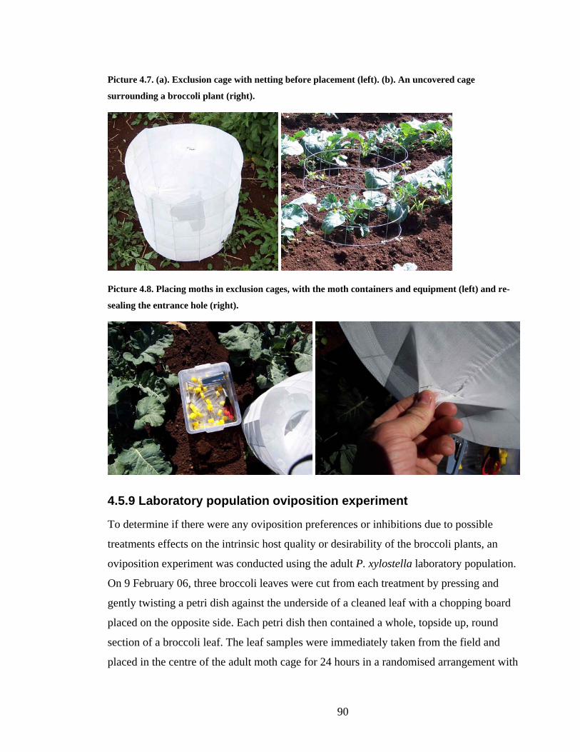
90
Picture 4.7. (a). Exclusion cage with netting before placement (left). (b). An uncovered cage
surrounding a broccoli plant (right).
Picture 4.8. Placing moths in exclusion cages, with the moth containers and equipment (left) and re-
sealing the entrance hole (right).
4.5.9 Laboratory population oviposition experiment
To determine if there were any oviposition preferences or inhibitions due to possible
treatments effects on the intrinsic host quality or desirability of the broccoli plants, an
oviposition experiment was conducted using the adult P. xylostella laboratory population.
On 9 February 06, three broccoli leaves were cut from each treatment by pressing and
gently twisting a petri dish against the underside of a cleaned leaf with a chopping board
placed on the opposite side. Each petri dish then contained a whole, topside up, round
section of a broccoli leaf. The leaf samples were immediately taken from the field and
placed in the centre of the adult moth cage for 24 hours in a randomised arrangement with

91
three replications (in three trays). A stereo-microscope was then used to count the eggs on
each leaf. The procedure was repeated on 14 and 21 February 06.
4.5.10 Semi commercial cover crop experiment 05/06
To determine if the cover crop results from the 04/05 experiment were valid at scales
greater than the plot size of 10m2, with the view of commercial implementation, a semi-
commercial planting of one hectare of broccoli was established on a farm at Gawler (E
429220, N 5440190) on Tasmania’s northwest coast. This location was 15km west of
Forthside Research Station and in a similar environment (climate and soil). The
experimental area was 50m wide and 200m long and divided into four plot pairs, each plot
being 25m x 50m. One plot in each pair was randomly designated to have either a cover
crop or to be prepared using conventional tillage (that is, bare soil). The rye cover crop was
sown on 17 August 05 at a rate of 100kg/ha without fertiliser. The cover crop was sprayed
and killed on 15 November 05 using glyphosate (720g ai/ha). Due to time constraints
brought on by developmental problems with the one-pass roller/ transplanter, only half the
area was planted with broccoli on 5 December, making each plot 12.5m wide and 50m
long. Again time constraints, in this instance associated with the management and sampling
regime of the Forthside trial, meant that for this experiment 15 randomly selected plants
from each plot were sampled once for the presence of P. xylostella eggs and larvae, P.
rapae larvae and B. brassicae colonies on 28 December (23 DAT). The trial was terminated
on 23 January.
4.5.11 Data analysis 04/05
The P. rapae and P. xylostella larvae and pupae counts from the 04/05 experiment were
analysed using a one-way analysis of variance (ANOVA) (Proc GLM, SAS Institute, Cary,
NC) for each sampling date. The mean counts from each plot were used as the response
variables, while the three replications (blocks) and the four treatments (treatments) were the
predictor variables. Treatment means were separated using Fisher’s least significant
difference (LSD) and data were log+1 transformed when necessary to conform to the
assumptions of the ANOVA procedure. However, only non-transformed data were reported
in the figures and tables.
92
The B. brassicae colony and parasitism data from the 04/05 experiment were based on the
proportion of plants infested. Therefore the data were arcsine square root transformed prior
to using the ANOVA procedure. These proportions were used as the response variables,
while the predictor variables were also the blocks and treatments.
To determine the effects of different treatments, pairwise contrasts were also planned for all
the insect data. These contrasts were performed using the ANOVA model so that the results
from the monoculture plots were compared to the results from the strip cropping plots; and
the results of the cover crop plots were compared to the bare soil plots.
The pairwise contrasts for 04/05 can be summarised as:
1. Cover crop vs. Bare soil
2. Strip crop vs. Monoculture
An example ANOVA table is presented as an appendix.
4.5.12 Data analysis 05/06
The P. rapae and P. xylostella egg, combined larvae and pupae counts and the P. xylostella
vacuum sampling data from the 05/06 experiment were analysed using a one-way ANOVA
(Proc GLM, SAS Institute, Cary, NC) for each sampling date. The mean counts from each
plot were used as the response variables, while the six columns (block) and the six rows
(row) of the Latin square design; and the six treatments (treatment) were the predictor
variables.
For the oviposition preference experiment, an ANOVA was also used to analyse the data.
The number of eggs oviposited were used as the response variable while each tray,
treatment and replication were used as the predictor variables.
For all ANOVA analyses, treatment means were separated using Fisher’s least significant
difference (LSD) and data were log+1 transformed when necessary to conform to the
assumptions of the ANOVA procedure. However, only non-transformed data were reported
in the figures and tables.
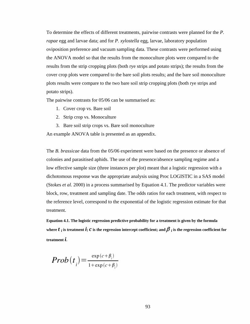
93
To determine the effects of different treatments, pairwise contrasts were planned for the P.
rapae egg and larvae data; and for P. xylostella egg, larvae, laboratory population
oviposition preference and vacuum sampling data. These contrasts were performed using
the ANOVA model so that the results from the monoculture plots were compared to the
results from the strip cropping plots (both rye strips and potato strips); the results from the
cover crop plots were compared to the bare soil plots results; and the bare soil monoculture
plots results were compare to the two bare soil strip cropping plots (both rye strips and
potato strips).
The pairwise contrasts for 05/06 can be summarised as:
1. Cover crop vs. Bare soil
2. Strip crop vs. Monoculture
3. Bare soil strip crops vs. Bare soil monoculture
An example ANOVA table is presented as an appendix.
The B. brassicae data from the 05/06 experiment were based on the presence or absence of
colonies and parasitised aphids. The use of the presence/absence sampling regime and a
low effective sample size (three instances per plot) meant that a logistic regression with a
dichotomous response was the appropriate analysis using Proc LOGISTIC in a SAS model
(Stokes et al. 2000) in a process summarised by Equation 4.1. The predictor variables were
block, row, treatment and sampling date. The odds ratios for each treatment, with respect to
the reference level, correspond to the exponential of the logistic regression estimate for that
treatment.
Equation 4.1. The logistic regression predictive probability for a treatment is given by the formula
where t i is treatment i; c is the regression intercept coefficient; and β i is the regression coefficient for
treatment i.
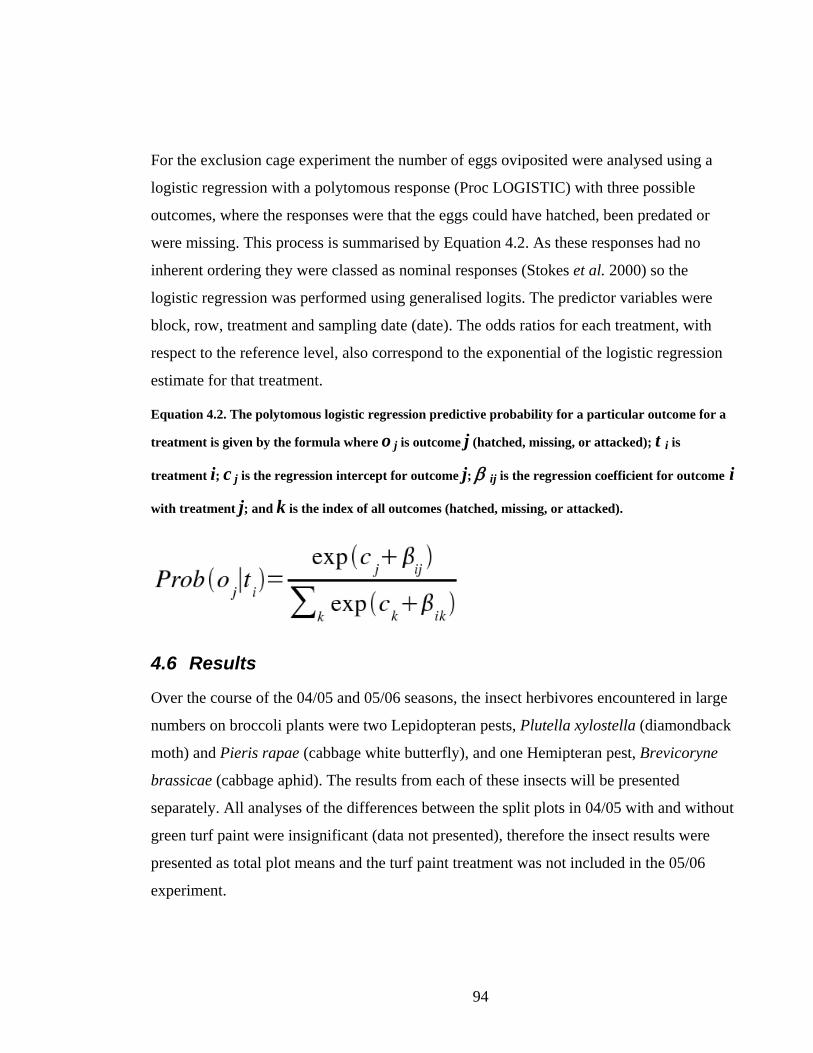
94
For the exclusion cage experiment the number of eggs oviposited were analysed using a
logistic regression with a polytomous response (Proc LOGISTIC) with three possible
outcomes, where the responses were that the eggs could have hatched, been predated or
were missing. This process is summarised by Equation 4.2. As these responses had no
inherent ordering they were classed as nominal responses (Stokes et al. 2000) so the
logistic regression was performed using generalised logits. The predictor variables were
block, row, treatment and sampling date (date). The odds ratios for each treatment, with
respect to the reference level, also correspond to the exponential of the logistic regression
estimate for that treatment.
Equation 4.2. The polytomous logistic regression predictive probability for a particular outcome for a
treatment is given by the formula where o j is outcome j (hatched, missing, or attacked); t i is
treatment i; c j is the regression intercept for outcome j; β ij is the regression coefficient for outcome i
with treatment j; and k is the index of all outcomes (hatched, missing, or attacked).
4.6 Results
Over the course of the 04/05 and 05/06 seasons, the insect herbivores encountered in large
numbers on broccoli plants were two Lepidopteran pests, Plutella xylostella (diamondback
moth) and Pieris rapae (cabbage white butterfly), and one Hemipteran pest, Brevicoryne
brassicae (cabbage aphid). The results from each of these insects will be presented
separately. All analyses of the differences between the split plots in 04/05 with and without
green turf paint were insignificant (data not presented), therefore the insect results were
presented as total plot means and the turf paint treatment was not included in the 05/06
experiment.

95
4.6.1 Meteorological data
Average meteorological data for temperature and rainfall for each of the trial seasons is
presented in Table 4.1. The biggest difference between the two seasons was the much
higher rainfall totals that occurred in the early part of the 05/06 season. As the experiments
were irrigated to prevent soil moisture from being a limiting factor, this would have had
little effect on plant performance in the different years. The main potential differences
stemming from the additional rainfall, might have been a reduction in local population of P.
xylostella in the 05/06 season prior to commencement of the experiment, as rainfall is a
significant mortality factor for this insect (Talekar and Shelton 1993). However, the
numbers of P. xylostella in the 05/06 experiment were on average the same or higher than
in the 04/05 experiment.
Table 4.1. Mean monthly meteorological data for Forthside from September to March in 04/05 and
05/06 with long term averages in brackets.
Month - Year Min. Temp. (degC) Max. Temp. (degC) Rainfall Total (mm)
September-04 5.7 (4.9) 14.2 (13.3) 30.4 (98.3)
October-04 6.9 (6.2) 15.8 (15.40) 52.4 (84.9)
November-04 9.0 (8.1) 17.5 (17.1) 84.8 (69.5)
December-04 10.6 (9.6) 20.4 (18.9) 35.8 (67.5)
January-05 11.7 (11.0) 21.0 (20.6) 14.8 (54.4)
February-05 12.2 (11.6) 21.7 (21.0) 0.4 (45.8)
March-05 9.4 (10.4) 19.6 (19.8) 3.8 (55.5)
September-05 5.2 (4.9) 13.6 (13.3) 117.2 (98.3)
October-05 8.8 (6.2) 15.6 (15.4) 225.0 (84.9)
November-05 9.7 (8.1) 17.8 (17.1) 162.0 (69.5)
December-05 10.7 (9.6) 19.1 (18.9) 113.4 (67.5)
January-06 11.9 (11.0) 21.4 (20.6) 26.0 (54.4)
February-06 11.3 (11.6) 21.4 (21.0) 8.0 (45.8)
March-06 10.8 (10.4) 20.5 (19.8) 23.2 (55.5)

96
4.6.2 Plutella xylostella (diamondback moth)
4.6.2.1 P. xylostella larvae and pupae numbers 04/05
P. xylostella larvae data from the 04/05 experiment indicate that there were significant
differences between the different treatments, which first became evident at 26 DAT and
continued until the final sample at 41 DAT (Figure 4.4). The LSD separations of the four
treatments, designated by the different letters on the graph, illustrates that the treatments
can be separated into two significantly different groups, with the two bare soil treatments
having higher numbers of P. xylostella larvae compared to the cover crop treatments. This
is further supported by the significance of the pairwise contrast of the cover crop and the
bare soil treatments indicating that from 19 DAT, there were significantly fewer P.
xylostella larvae in the cover crop treatments (Table 4.2). The results also indicate that apart
from 19 DAT, there were no significant differences between strip cropping treatments and
monoculture plots.
Figure 4.4. The mean number of P. xylostella larvae per plant sampled in 04/05 ± SE. “ns” not
significant; * P ≤ 0.05; ** P ≤ 0.01; *** P ≤ 0.001. Points without a letter in common are significantly
different (P=0.05).
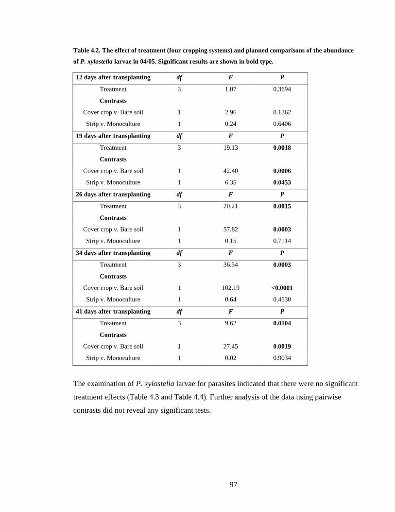
97
Table 4.2. The effect of treatment (four cropping systems) and planned comparisons of the abundance
of P. xylostella larvae in 04/05. Significant results are shown in bold type.
12 days after transplanting df F P
Treatment 3 1.07 0.3694
Contrasts
Cover crop v. Bare soil 1 2.96 0.1362
Strip v. Monoculture 1 0.24 0.6406
19 days after transplanting df F P
Treatment 3 19.13 0.0018
Contrasts
Cover crop v. Bare soil 1 42.40 0.0006
Strip v. Monoculture 1 6.35 0.0453
26 days after transplanting df F P
Treatment 3 20.21 0.0015
Contrasts
Cover crop v. Bare soil 1 57.82 0.0003
Strip v. Monoculture 1 0.15 0.7114
34 days after transplanting df F P
Treatment 3 36.54 0.0003
Contrasts
Cover crop v. Bare soil 1 102.19 <0.0001
Strip v. Monoculture 1 0.64 0.4530
41 days after transplanting df F P
Treatment 3 9.62 0.0104
Contrasts
Cover crop v. Bare soil 1 27.45 0.0019
Strip v. Monoculture 1 0.02 0.9034
The examination of P. xylostella larvae for parasites indicated that there were no significant
treatment effects (Table 4.3 and Table 4.4). Further analysis of the data using pairwise
contrasts did not reveal any significant tests.
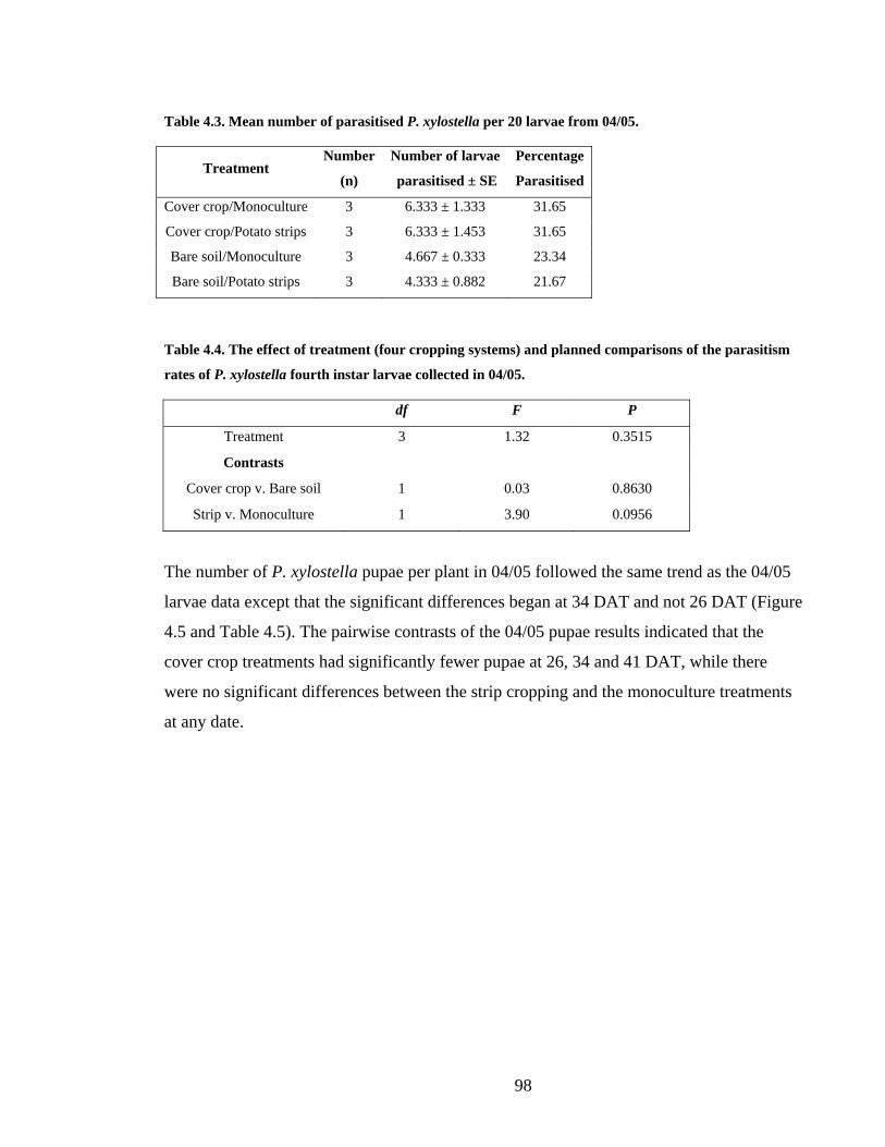
98
Table 4.3. Mean number of parasitised P. xylostella per 20 larvae from 04/05.
Treatment Number
(n)
Number of larvae
parasitised ± SE
Percentage
Parasitised
Cover crop/Monoculture 3 6.333 ± 1.333 31.65
Cover crop/Potato strips 3 6.333 ± 1.453 31.65
Bare soil/Monoculture 3 4.667 ± 0.333 23.34
Bare soil/Potato strips 3 4.333 ± 0.882 21.67
Table 4.4. The effect of treatment (four cropping systems) and planned comparisons of the parasitism
rates of P. xylostella fourth instar larvae collected in 04/05.
df F P
Treatment 3 1.32 0.3515
Contrasts
Cover crop v. Bare soil 1 0.03 0.8630
Strip v. Monoculture 1 3.90 0.0956
The number of P. xylostella pupae per plant in 04/05 followed the same trend as the 04/05
larvae data except that the significant differences began at 34 DAT and not 26 DAT (Figure
4.5 and Table 4.5). The pairwise contrasts of the 04/05 pupae results indicated that the
cover crop treatments had significantly fewer pupae at 26, 34 and 41 DAT, while there
were no significant differences between the strip cropping and the monoculture treatments
at any date.
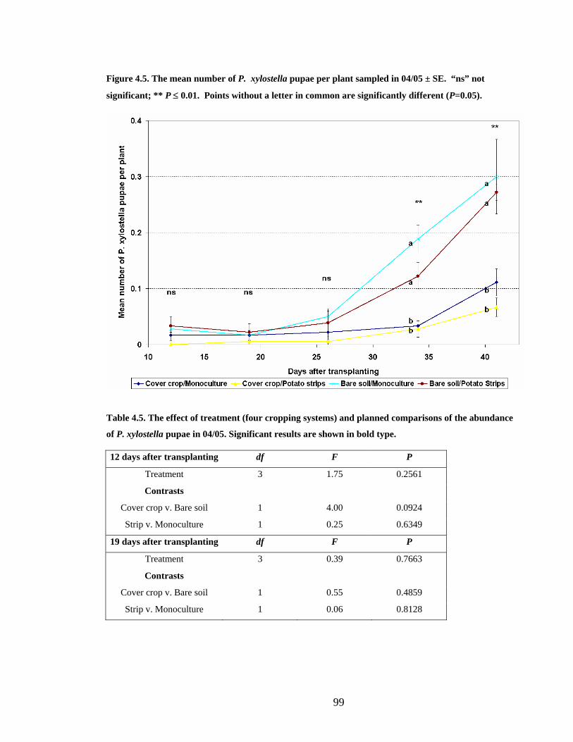
99
Figure 4.5. The mean number of P. xylostella pupae per plant sampled in 04/05 ± SE. “ns” not
significant; ** P ≤ 0.01. Points without a letter in common are significantly different (P=0.05).
Table 4.5. The effect of treatment (four cropping systems) and planned comparisons of the abundance
of P. xylostella pupae in 04/05. Significant results are shown in bold type.
12 days after transplanting df F P
Treatment 3 1.75 0.2561
Contrasts
Cover crop v. Bare soil 1 4.00 0.0924
Strip v. Monoculture 1 0.25 0.6349
19 days after transplanting df F P
Treatment 3 0.39 0.7663
Contrasts
Cover crop v. Bare soil 1 0.55 0.4859
Strip v. Monoculture 1 0.06 0.8128
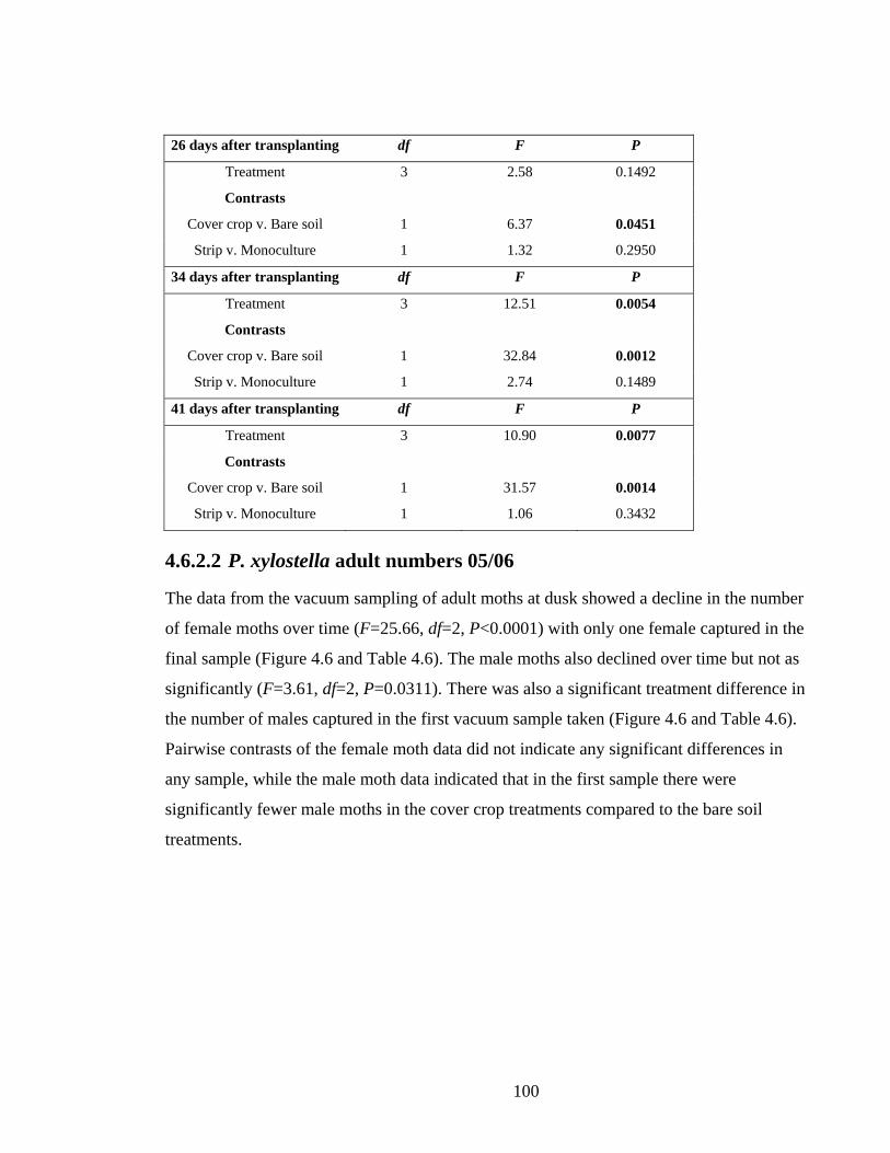
100
26 days after transplanting df F P
Treatment 3 2.58 0.1492
Contrasts
Cover crop v. Bare soil 1 6.37 0.0451
Strip v. Monoculture 1 1.32 0.2950
34 days after transplanting df F P
Treatment 3 12.51 0.0054
Contrasts
Cover crop v. Bare soil 1 32.84 0.0012
Strip v. Monoculture 1 2.74 0.1489
41 days after transplanting df F P
Treatment 3 10.90 0.0077
Contrasts
Cover crop v. Bare soil 1 31.57 0.0014
Strip v. Monoculture 1 1.06 0.3432
4.6.2.2 P. xylostella adult numbers 05/06
The data from the vacuum sampling of adult moths at dusk showed a decline in the number
of female moths over time (F=25.66, df=2, P<0.0001) with only one female captured in the
final sample (Figure 4.6 and Table 4.6). The male moths also declined over time but not as
significantly (F=3.61, df=2, P=0.0311). There was also a significant treatment difference in
the number of males captured in the first vacuum sample taken (Figure 4.6 and Table 4.6).
Pairwise contrasts of the female moth data did not indicate any significant differences in
any sample, while the male moth data indicated that in the first sample there were
significantly fewer male moths in the cover crop treatments compared to the bare soil
treatments.
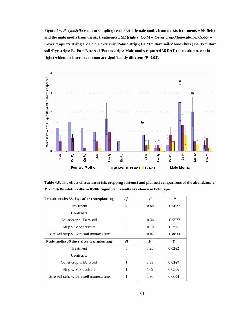
101
Figure 4.6. P. xylostella vacuum sampling results with female moths from the six treatments ± SE (left)
and the male moths from the six treatments ± SE (right). Cc-M = Cover crop/Monoculture; Cc-Ry =
Cover crop/Rye strips; Cc-Po = Cover crop/Potato strips; Bs-M = Bare soil/Monoculture; Bs-Ry = Bare
soil /Rye strips; Bs-Po = Bare soil /Potato strips; Male moths captured 36 DAT (blue columns on the
right) without a letter in common are significantly different (P=0.05).
Table 4.6. The effect of treatment (six cropping systems) and planned comparisons of the abundance of
P. xylostella adult moths in 05/06. Significant results are shown in bold type.
Female moths 36 days after transplanting df F P
Treatment 5 0.80 0.5627
Contrasts
Cover crop v. Bare soil 1 0.36 0.5577
Strip v. Monoculture 1 0.10 0.7551
Bare soil strip v. Bare soil monoculture 1 0.02 0.8830
Male moths 36 days after transplanting df F P
Treatment 5 3.25 0.0262
Contrasts
Cover crop v. Bare soil 1 6.83 0.0167
Strip v. Monoculture 1 4.09 0.0566
Bare soil strip v. Bare soil monoculture 1 3.96 0.0604
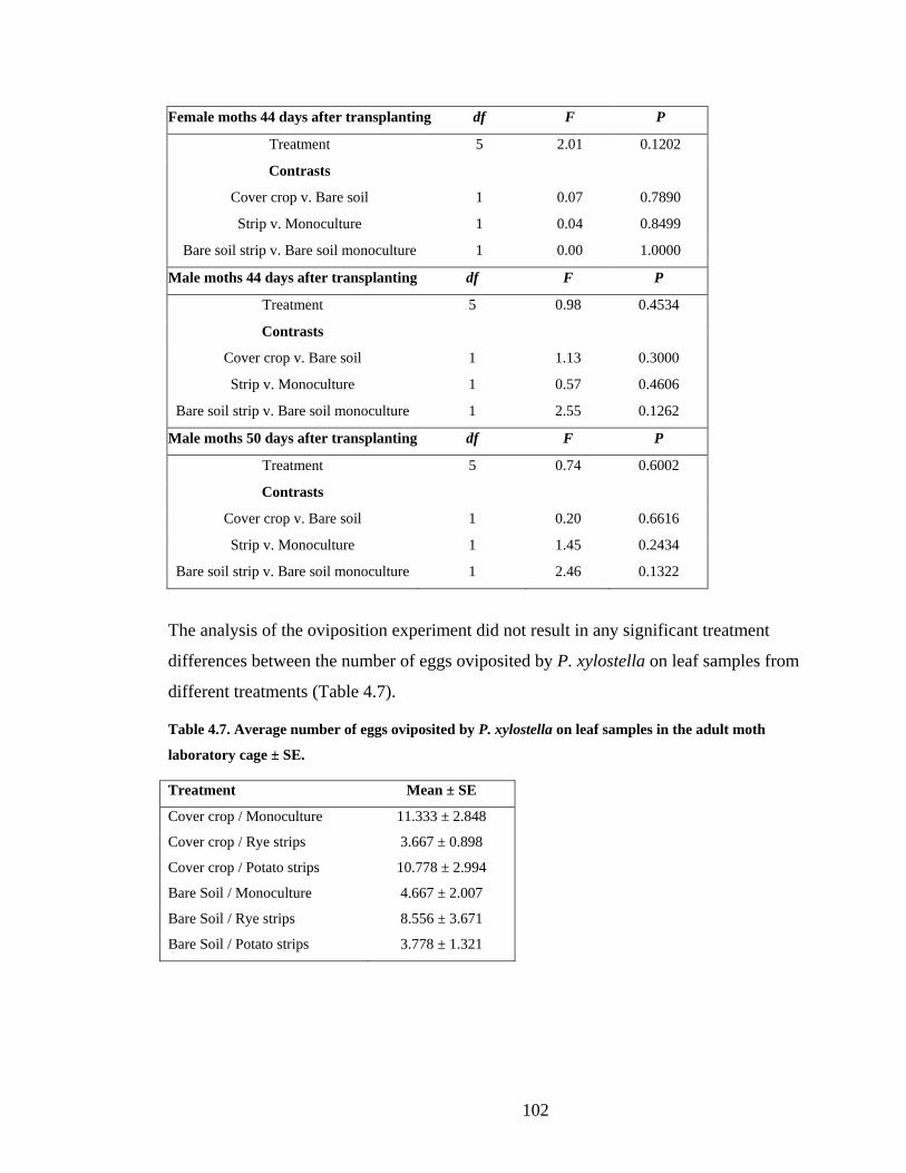
102
Female moths 44 days after transplanting df F P
Treatment 5 2.01 0.1202
Contrasts
Cover crop v. Bare soil 1 0.07 0.7890
Strip v. Monoculture 1 0.04 0.8499
Bare soil strip v. Bare soil monoculture 1 0.00 1.0000
Male moths 44 days after transplanting df F P
Treatment 5 0.98 0.4534
Contrasts
Cover crop v. Bare soil 1 1.13 0.3000
Strip v. Monoculture 1 0.57 0.4606
Bare soil strip v. Bare soil monoculture 1 2.55 0.1262
Male moths 50 days after transplanting df F P
Treatment 5 0.74 0.6002
Contrasts
Cover crop v. Bare soil 1 0.20 0.6616
Strip v. Monoculture 1 1.45 0.2434
Bare soil strip v. Bare soil monoculture 1 2.46 0.1322
The analysis of the oviposition experiment did not result in any significant treatment
differences between the number of eggs oviposited by P. xylostella on leaf samples from
different treatments (Table 4.7).
Table 4.7. Average number of eggs oviposited by P. xylostella on leaf samples in the adult moth
laboratory cage ± SE.
Treatment Mean ± SE
Cover crop / Monoculture 11.333 ± 2.848
Cover crop / Rye strips 3.667 ± 0.898
Cover crop / Potato strips 10.778 ± 2.994
Bare Soil / Monoculture 4.667 ± 2.007
Bare Soil / Rye strips 8.556 ± 3.671
Bare Soil / Potato strips 3.778 ± 1.321
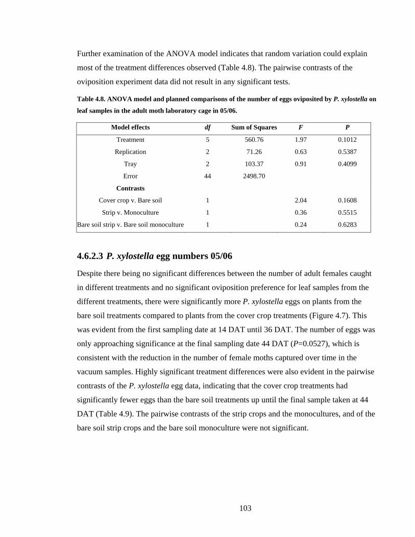
103
Further examination of the ANOVA model indicates that random variation could explain
most of the treatment differences observed (Table 4.8). The pairwise contrasts of the
oviposition experiment data did not result in any significant tests.
Table 4.8. ANOVA model and planned comparisons of the number of eggs oviposited by P. xylostella on
leaf samples in the adult moth laboratory cage in 05/06.
Model effects df Sum of Squares F P
Treatment 5 560.76 1.97 0.1012
Replication 2 71.26 0.63 0.5387
Tray 2 103.37 0.91 0.4099
Error 44 2498.70
Contrasts
Cover crop v. Bare soil 1 2.04 0.1608
Strip v. Monoculture 1 0.36 0.5515
Bare soil strip v. Bare soil monoculture 1 0.24 0.6283
4.6.2.3 P. xylostella egg numbers 05/06
Despite there being no significant differences between the number of adult females caught
in different treatments and no significant oviposition preference for leaf samples from the
different treatments, there were significantly more P. xylostella eggs on plants from the
bare soil treatments compared to plants from the cover crop treatments (Figure 4.7). This
was evident from the first sampling date at 14 DAT until 36 DAT. The number of eggs was
only approaching significance at the final sampling date 44 DAT (P=0.0527), which is
consistent with the reduction in the number of female moths captured over time in the
vacuum samples. Highly significant treatment differences were also evident in the pairwise
contrasts of the P. xylostella egg data, indicating that the cover crop treatments had
significantly fewer eggs than the bare soil treatments up until the final sample taken at 44
DAT (Table 4.9). The pairwise contrasts of the strip crops and the monocultures, and of the
bare soil strip crops and the bare soil monoculture were not significant.

104
Figure 4.7. The mean number of P. xylostella eggs per plant sampled in 05/06 ± SE. “ns” not
significant; * P ≤ 0.05; ** P ≤ 0.01; *** P ≤ 0.001. Points without a letter in common are significantly
different (P=0.05).
Table 4.9. The effect of treatment (six cropping systems) and planned comparisons of the abundance of
P. xylostella eggs in 05/06. Significant results are shown in bold type.
14 days after transplanting df F P
Treatment 5 6.93 0.0007
Contrasts
Cover crop v. Bare soil 1 29.62 <0.0001
Strip v. Monoculture 1 0.89 0.3565
Bare soil strip v. Bare soil monoculture 1 1.92 0.1810
22 days after transplanting df F P
Treatment 5 4.79 0.0048
Contrasts
Cover crop v. Bare soil 1 22.71 0.0001
Strip v. Monoculture 1 0.28 0.6027
Bare soil strip v. Bare soil monoculture 1 0.52 0.4783
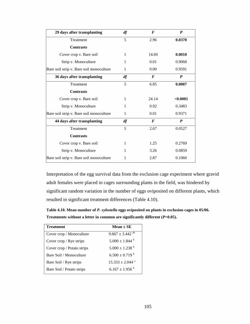
105
29 days after transplanting df F P
Treatment 5 2.96 0.0370
Contrasts
Cover crop v. Bare soil 1 14.69 0.0010
Strip v. Monoculture 1 0.01 0.9068
Bare soil strip v. Bare soil monoculture 1 0.00 0.9591
36 days after transplanting df F P
Treatment 5 6.85 0.0007
Contrasts
Cover crop v. Bare soil 1 24.14 <0.0001
Strip v. Monoculture 1 0.92 0.3483
Bare soil strip v. Bare soil monoculture 1 0.01 0.9371
44 days after transplanting df F P
Treatment 5 2.67 0.0527
Contrasts
Cover crop v. Bare soil 1 1.25 0.2769
Strip v. Monoculture 1 3.26 0.0859
Bare soil strip v. Bare soil monoculture 1 2.87 0.1060
Interpretation of the egg survival data from the exclusion cage experiment where gravid
adult females were placed in cages surrounding plants in the field, was hindered by
significant random variation in the number of eggs oviposited on different plants, which
resulted in significant treatment differences (Table 4.10).
Table 4.10. Mean number of P. xylostella eggs oviposited on plants in exclusion cages in 05/06.
Treatments without a letter in common are significantly different (P=0.05).
Treatment Mean ± SE
Cover crop / Monoculture 9.667 ± 3.442 ab
Cover crop / Rye strips 5.000 ± 1.844 b
Cover crop / Potato strips 5.000 ± 1.238 b
Bare Soil / Monoculture 6.500 ± 0.719 b
Bare Soil / Rye strips 15.333 ± 2.044 a
Bare Soil / Potato strips 6.167 ± 1.956 b

106
When the treatments were separated using Fisher’s LSD, the Bare soil/Rye strips treatment
had significantly more eggs oviposited than all other treatments except the Cover
crop/Monoculture. However, unlike the other P. xylostella data there were no apparent
treatment groupings, which resulted in no significant contrasts (Table 4.11).
Table 4.11. The effect of treatment (six cropping systems) and planned comparisons of the abundance
of P. xylostella eggs oviposited on plants in exclusion cages in 05/06. Significant results are shown in
bold type.
df F P
Treatment 5 3.68 0.0159
Contrasts
Cover crop v. Bare soil 1 2.66 0.1186
Strip v. Monoculture 1 0.01 0.9093
Bare soil strip v. Bare soil monoculture 1 2.77 0.1118
Despite the differences in the number of eggs across treatments, the analysis of the caged
egg survival data indicated that: eggs oviposited in the Cover crop/Monoculture treatment
were approximately 2.7 times more likely to be attacked than hatched and 3.3 times more
likely to be missing than hatched; eggs oviposited in the Cover crop/Rye strips treatment
were approximately 3.3 times less likely to be attacked than hatched and 3.6 times more
likely to be missing than hatched; and eggs oviposited in the Bare soil/Rye strips treatment
were approximately 2.0 times more likely to be attacked than hatched and 2.2 times less
likely to be missing than attacked (Table 4.12).
There were no eggs recovered from the second egg experiment where eggs from the
laboratory population were placed on plants in the field. There was approximately 2mm of
rainfall in the period between placing the eggs in the field and the assessment, which
combined with slight changes in leaf angle from the horizontal may have been enough to
wash the eggs from the plants.

107
Table 4.12. Comparison of outcomes for P. xylostella eggs oviposited in the exclusion cage experiment.
Treatment Comparison Estimate LikelihoodStandard
Error
Wald
Chi-SquareP
Attacked v. Hatched 1.004 2.729 0.413 5.914 0.0150
Missing v. Hatched 1.185 3.271 0.405 8.564 0.0034Cover Crop Monoculture
Missing v. Attacked 0.181 0.386 0.220 0.6387
Attacked v. Hatched -1.188 3.280 0.591 4.044 0.0443
Missing v. Hatched 0.087 0.467 0.035 0.8525Cover Crop Rye Strips
Missing v. Attacked 1.275 3.579 0.6302 4.094 0.0430
Attacked v. Hatched -0.742 0.475 2.440 0.1183
Missing v. Hatched -0.397 0.457 0.756 0.3846Cover Crop Potato Strips
Missing v. Attacked 0.345 0.5339 0.417 0.5183
Attacked v. Hatched 0.128 0.409 0.097 0.7550
Missing v. Hatched -0.244 0.401 0.373 0.5415Bare Soil Monoculture
Missing v. Attacked -0.372 0.4266 0.762 0.3827
Attacked v. Hatched 0.687 1.988 0.318 4.669 0.0307
Missing v. Hatched -0.083 0.323 0.065 0.7983Bare Soil Rye Strips
Missing v. Attacked -0.770 2.160 0.3301 5.438 0.0197
Attacked v. Hatched 0.112 0.402 0.077 0.7808
Missing v. Hatched -0.547 0.467 1.373 0.2414Bare Soil Potato Strips
Missing v. Attacked -0.6509 0.4966 1.760 0.1846
When these results were expressed graphically it becomes more evident that there was a
low probability of eggs hatching in the Cover crop/Monoculture treatment, a low
probability of eggs being attacked in the Cover crop/Rye strips treatment and a high
probability of eggs being attacked in the Bare soil/Rye strips treatment (Figure 4.8). Eggs in
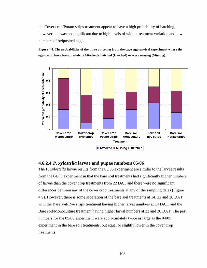
108
the Cover crop/Potato strips treatment appear to have a high probability of hatching,
however this was not significant due to high levels of within treatment variation and low
numbers of oviposited eggs.
Figure 4.8. The probabilities of the three outcomes from the cage egg survival experiment where the
eggs could have been predated (Attacked), hatched (Hatched) or were missing (Missing).
4.6.2.4 P. xylostella larvae and pupae numbers 05/06 The P. xylostella larvae results from the 05/06 experiment are similar to the larvae results
from the 04/05 experiment in that the bare soil treatments had significantly higher numbers
of larvae than the cover crop treatments from 22 DAT and there were no significant
differences between any of the cover crop treatments at any of the sampling dates (Figure
4.9). However, there is some separation of the bare soil treatments at 14, 22 and 36 DAT,
with the Bare soil/Rye strips treatment having higher larval numbers at 14 DAT, and the
Bare soil/Monoculture treatment having higher larval numbers at 22 and 36 DAT. The pest
numbers for the 05/06 experiment were approximately twice as large as the 04/05
experiment in the bare soil treatments, but equal or slightly lower in the cover crop
treatments.

109
Figure 4.9. The mean number of P. xylostella larvae per plant sampled in 05/06 ± SE. “ns” not
significant; * P ≤ 0.05; ** P ≤ 0.01; *** P ≤ 0.001. Points without a letter in common are significantly
different (P=0.05).
The pairwise contrasts of the 05/06 larval data again indicate that the cover cropping
treatments had significantly fewer P. xylostella larvae at all but the first sampling date
(Table 4.13). The pairwise contrasts also indicate that the strip cropping treatments had
significantly fewer larvae than the monoculture treatments at 22 DAT, largely due to the
high number of larvae in the Bare soil/Monoculture plots. The bare soil strip cropping
treatments (potato and rye) had significantly fewer larvae compared to the Bare
soil/Monoculture treatment at 22, 36 and 44 DAT.
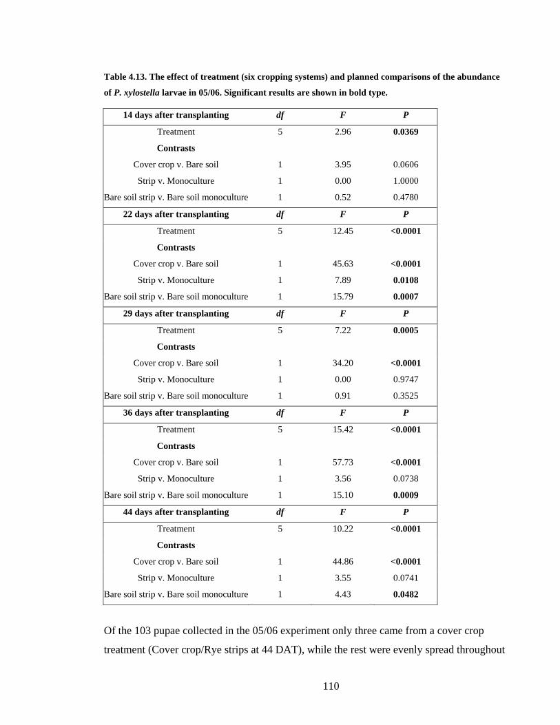
110
Table 4.13. The effect of treatment (six cropping systems) and planned comparisons of the abundance
of P. xylostella larvae in 05/06. Significant results are shown in bold type.
14 days after transplanting df F P
Treatment 5 2.96 0.0369
Contrasts
Cover crop v. Bare soil 1 3.95 0.0606
Strip v. Monoculture 1 0.00 1.0000
Bare soil strip v. Bare soil monoculture 1 0.52 0.4780
22 days after transplanting df F P
Treatment 5 12.45 <0.0001
Contrasts
Cover crop v. Bare soil 1 45.63 <0.0001
Strip v. Monoculture 1 7.89 0.0108
Bare soil strip v. Bare soil monoculture 1 15.79 0.0007
29 days after transplanting df F P
Treatment 5 7.22 0.0005
Contrasts
Cover crop v. Bare soil 1 34.20 <0.0001
Strip v. Monoculture 1 0.00 0.9747
Bare soil strip v. Bare soil monoculture 1 0.91 0.3525
36 days after transplanting df F P
Treatment 5 15.42 <0.0001
Contrasts
Cover crop v. Bare soil 1 57.73 <0.0001
Strip v. Monoculture 1 3.56 0.0738
Bare soil strip v. Bare soil monoculture 1 15.10 0.0009
44 days after transplanting df F P
Treatment 5 10.22 <0.0001
Contrasts
Cover crop v. Bare soil 1 44.86 <0.0001
Strip v. Monoculture 1 3.55 0.0741
Bare soil strip v. Bare soil monoculture 1 4.43 0.0482
Of the 103 pupae collected in the 05/06 experiment only three came from a cover crop
treatment (Cover crop/Rye strips at 44 DAT), while the rest were evenly spread throughout

111
the remaining bare soil treatments with no significant differences between them (F=0.59,
df=2, P=0.5587). All pupae collected were parasitised, with 101 Diadegma sp. (D.
semiclausum (Hellén) and D. rapi (Cameron), Hymenoptera: Ichneumonidae) adults
emerging and two Diadromus collaris (Gravenhorst, Hymenoptera: Ichneumonidae) adults.
The P. xylostella population summary from the 05/06 experiment, indicates that there were
fewer eggs in the cover crop treatments when compared to the bare soil treatments,
resulting in fewer larvae at all the recorded instars with virtually none pupating (Figure
4.10).
Figure 4.10. P. xylostella populations at each 05/06 sample as eggs, 1st, 2nd, 3rd and 4th instars or pupae.
4.6.3 Pieris rapae (cabbage white butterfly)
4.6.3.1 P. rapae larvae numbers 04/05
The P. rapae larvae data from 04/05 differ from the 04/05 P. xylostella data in that there
were no apparent differences between treatments as the larvae numbers generally increased
over time in all treatments (Figure 4.11).

112
Figure 4.11. The mean number of P. rapae larvae per plant sampled in 04/05 ± SE. “ns” not significant;
* P ≤ 0.05. Points without a letter in common are significantly different (P=0.05).
However, there was a significant difference between the number of P. rapae larvae in the
different treatments on the last sampling date at 41 DAT, with the Cover crop/Potato strips
treatment being higher than both the monoculture treatments. This difference, when
combined with the Bare soil/Potato strips data in the pairwise contrasts, led to a significant
test at 41 DAT when the strip crops were compared to the monoculture plots. This meant
that on the final sampling date, there were significantly more P. rapae larvae in the strip
cropping plots compared to the monoculture plots (Table 4.14).
Table 4.14. The effect of treatment (four cropping systems) and planned comparisons of the abundance
of P. rapae larvae in 04/05. Significant results are shown in bold type.
12 days after transplanting df F P
Treatment 3 3.30 0.0995
Contrasts
Cover crop v. Bare soil 1 5.17 0.0633
Strip v. Monoculture 1 3.13 0.1274
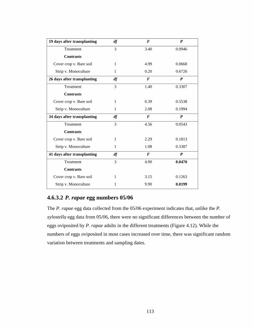
113
19 days after transplanting df F P
Treatment 3 3.40 0.0946
Contrasts
Cover crop v. Bare soil 1 4.99 0.0668
Strip v. Monoculture 1 0.20 0.6726
26 days after transplanting df F P
Treatment 3 1.40 0.3307
Contrasts
Cover crop v. Bare soil 1 0.39 0.5538
Strip v. Monoculture 1 2.08 0.1994
34 days after transplanting df F P
Treatment 3 4.56 0.0543
Contrasts
Cover crop v. Bare soil 1 2.29 0.1813
Strip v. Monoculture 1 1.08 0.3387
41 days after transplanting df F P
Treatment 3 4.90 0.0470
Contrasts
Cover crop v. Bare soil 1 3.15 0.1263
Strip v. Monoculture 1 9.90 0.0199
4.6.3.2 P. rapae egg numbers 05/06
The P. rapae egg data collected from the 05/06 experiment indicates that, unlike the P.
xylostella egg data from 05/06, there were no significant differences between the number of
eggs oviposited by P. rapae adults in the different treatments (Figure 4.12). While the
numbers of eggs oviposited in most cases increased over time, there was significant random
variation between treatments and sampling dates.

114
Figure 4.12. The mean number of P. rapae eggs per plant sampled in 05/06 ± SE. “ns” indicates that
there were no significant differences for that sampling date.
Although there were no significant differences evident in the number of P. rapae eggs
oviposited in each treatment, pairwise contrasts of the data resulted in two significant tests.
The Bare soil/Monoculture treatment had a substantial reduction in the number of eggs
between the samples collected 36DAT and 44DAT, which explains why the cover crop
treatments had significantly higher egg numbers than the bare soil treatments at 44 DAT.
Conversely, the low number of eggs in the Cover crop/Monoculture treatment at 22 DAT,
resulted in the monoculture treatments having significantly fewer eggs than the strip crop
treatments at 22 DAT.
Table 4.15. The effect of treatment (six cropping systems) and planned comparisons of the abundance
of P. rapae eggs in 05/06. Significant results are shown in bold type.
14 days after transplanting df F P
Treatment 5 0.50 0.7703
Contrasts
Cover crop v. Bare soil 1 0.72 0.4072
Strip v. Monoculture 1 0.00 0.9540
Bare soil strip v. Bare soil monoculture 1 0.74 0.4001

115
22 days after transplanting df F P
Treatment 5 2.30 0.0830
Contrasts
Cover crop v. Bare soil 1 1.77 0.1984
Strip v. Monoculture 1 6.11 0.0226
Bare soil strip v. Bare soil monoculture 1 3.93 0.0613
29 days after transplanting df F P
Treatment 5 0.96 0.4639
Contrasts
Cover crop v. Bare soil 1 1.49 0.2357
Strip v. Monoculture 1 3.08 0.0944
Bare soil strip v. Bare soil monoculture 1 0.99 0.3324
36 days after transplanting df F P
Treatment 5 0.76 0.5922
Contrasts
Cover crop v. Bare soil 1 0.79 0.3858
Strip v. Monoculture 1 0.90 0.3538
Bare soil strip v. Bare soil monoculture 1 1.24 0.2782
44 days after transplanting df F P
Treatment 5 2.10 0.1078
Contrasts
Cover crop v. Bare soil 1 8.42 0.0088
Strip v. Monoculture 1 1.56 0.2263
Bare soil strip v. Bare soil monoculture 1 1.29 0.2694
4.6.3.3 P. rapae larvae numbers 05/06
The P. rapae larvae results from the 05/06 experiment show a similar trend to the 04/05 P.
rapae results, with a steady increase in larvae numbers over time (Figure 4.13). Unlike the
P. xylostella larvae data from both 04/05 and 05/06, there are no obvious treatment
differences or treatment groupings. It should also be noted that the numbers of P. rapae
larvae at each sampling date were approximately five times higher in 05/06 than the
previous season.

116
Figure 4.13. The mean number of P. rapae larvae per plant sampled in 05/06 ± SE. “ns” not significant;
* P ≤ 0.05. Points without a letter in common are significantly different (P=0.05).
There was a significant treatment difference at 36 DAT. This difference was also reflected
in the two significant pairwise contrasts at the same sampling date, with the cover crop
treatments having fewer P. rapae larvae than the bare soil treatments and the monoculture
treatments having fewer than the strip cropping treatments (Table 4.16).
Table 4.16. The effect of treatment (six cropping systems) and planned comparisons of the abundance
of P. rapae larvae in 05/06. Significant results are shown in bold type.
14 days after transplanting df F P
Treatment 5 0.39 0.8478
Contrasts
Cover crop v. Bare soil 1 0.18 0.6801
Strip v. Monoculture 1 0.16 0.6974
Bare soil strip v. Bare soil monoculture 1 0.31 0.5831
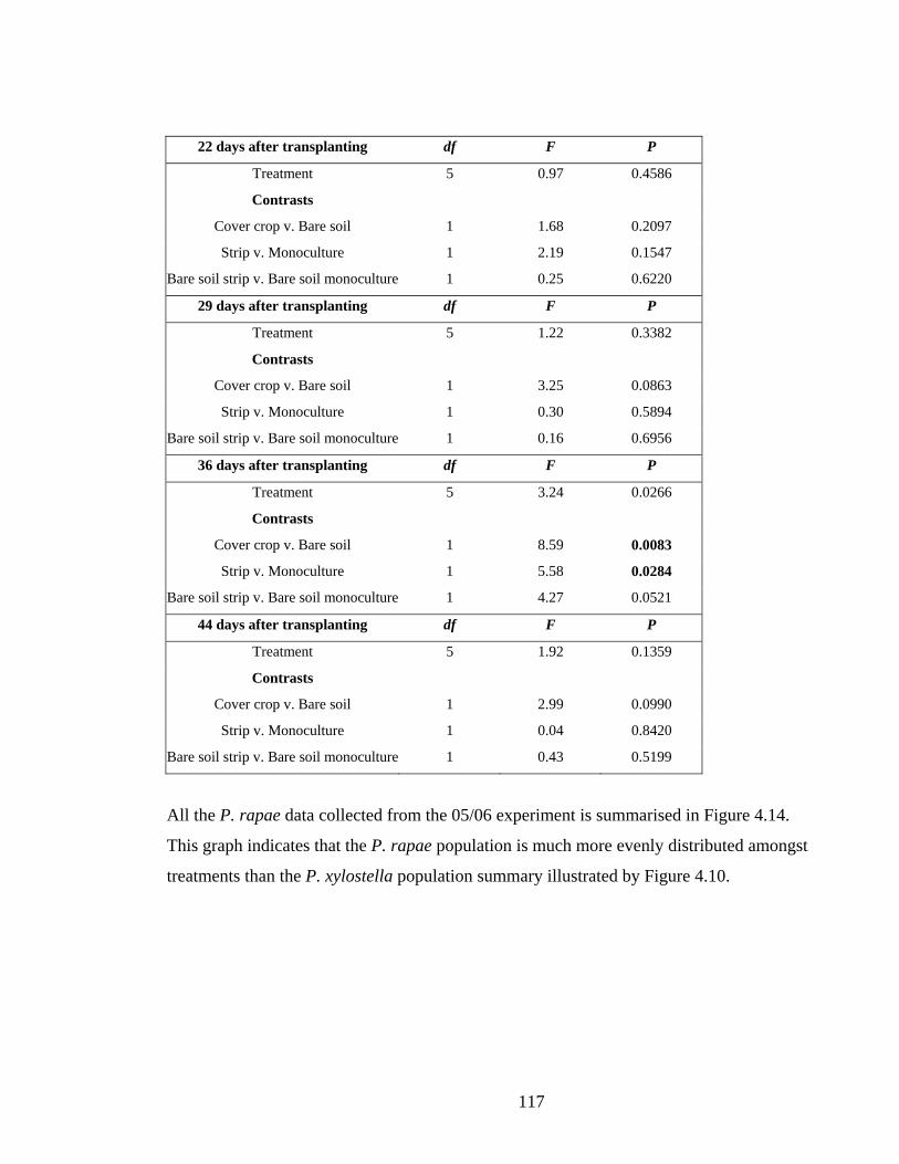
117
22 days after transplanting df F P
Treatment 5 0.97 0.4586
Contrasts
Cover crop v. Bare soil 1 1.68 0.2097
Strip v. Monoculture 1 2.19 0.1547
Bare soil strip v. Bare soil monoculture 1 0.25 0.6220
29 days after transplanting df F P
Treatment 5 1.22 0.3382
Contrasts
Cover crop v. Bare soil 1 3.25 0.0863
Strip v. Monoculture 1 0.30 0.5894
Bare soil strip v. Bare soil monoculture 1 0.16 0.6956
36 days after transplanting df F P
Treatment 5 3.24 0.0266
Contrasts
Cover crop v. Bare soil 1 8.59 0.0083
Strip v. Monoculture 1 5.58 0.0284
Bare soil strip v. Bare soil monoculture 1 4.27 0.0521
44 days after transplanting df F P
Treatment 5 1.92 0.1359
Contrasts
Cover crop v. Bare soil 1 2.99 0.0990
Strip v. Monoculture 1 0.04 0.8420
Bare soil strip v. Bare soil monoculture 1 0.43 0.5199
All the P. rapae data collected from the 05/06 experiment is summarised in Figure 4.14.
This graph indicates that the P. rapae population is much more evenly distributed amongst
treatments than the P. xylostella population summary illustrated by Figure 4.10.

118
Figure 4.14. P. rapae populations at each 05/06 sampling date summarised as: eggs; 1st and 2nd instar
(small) ; 3rd and 4th instars (medium); 5th instar (large); and pupae.
P. rapae pupae were first recorded on the 4th census date in both the 04/05 and 05/06
seasons and due to the low numbers recorded (29 in 2004/2005 and 21 in 2005/2006) pupal
data from P. rapae could not be statistically analysed and are not presented. The low
number of P. rapae pupae present in both seasons could be due to movement of P. rapae
larvae into neighbouring plant material or crops, therefore avoiding detection, as P. rapae
will move from the natal plant to pupate (Waterhouse and Sands 2001). This is
demonstrated in a picture taken in the strip cropping trial conducted in 2003/2004, where a
P. rapae larva has moved from a broccoli plant and pupated on a neighbouring onion plant
(Picture 4.9).
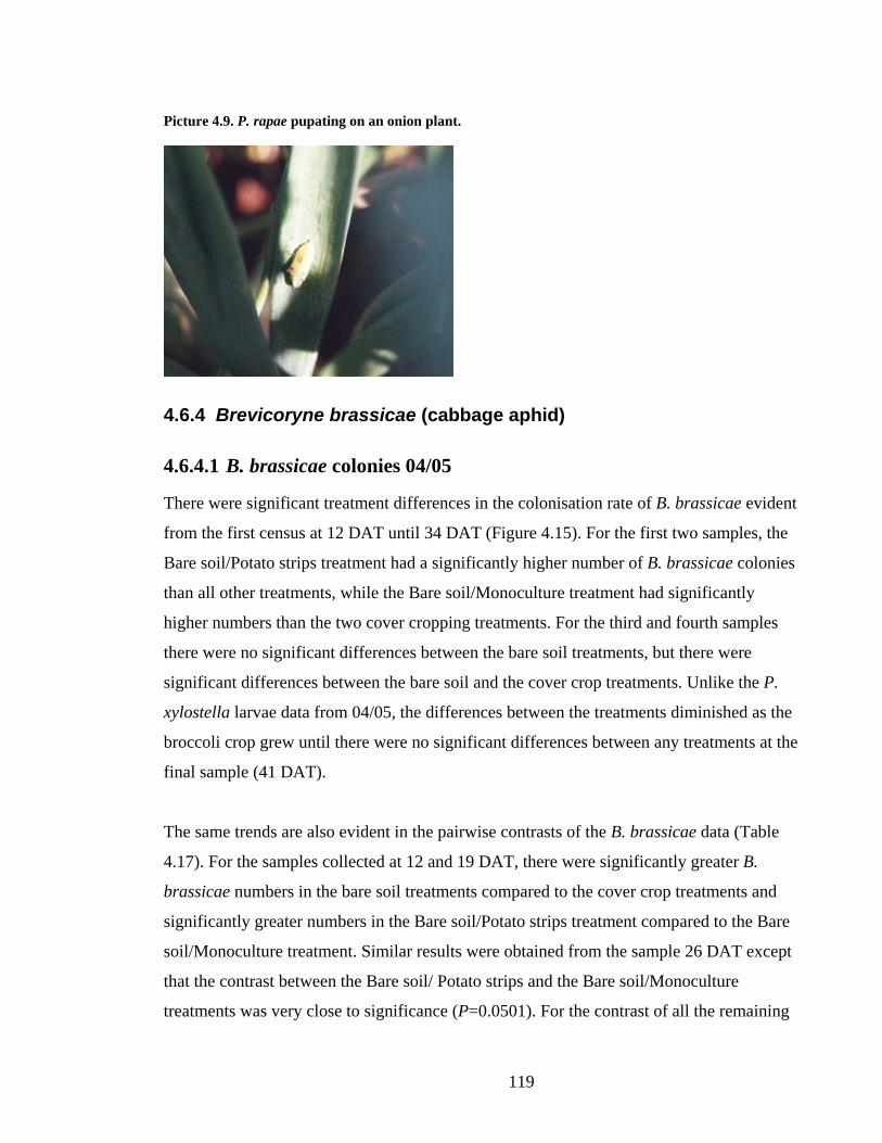
119
Picture 4.9. P. rapae pupating on an onion plant.
4.6.4 Brevicoryne brassicae (cabbage aphid)
4.6.4.1 B. brassicae colonies 04/05
There were significant treatment differences in the colonisation rate of B. brassicae evident
from the first census at 12 DAT until 34 DAT (Figure 4.15). For the first two samples, the
Bare soil/Potato strips treatment had a significantly higher number of B. brassicae colonies
than all other treatments, while the Bare soil/Monoculture treatment had significantly
higher numbers than the two cover cropping treatments. For the third and fourth samples
there were no significant differences between the bare soil treatments, but there were
significant differences between the bare soil and the cover crop treatments. Unlike the P.
xylostella larvae data from 04/05, the differences between the treatments diminished as the
broccoli crop grew until there were no significant differences between any treatments at the
final sample (41 DAT).
The same trends are also evident in the pairwise contrasts of the B. brassicae data (Table
4.17). For the samples collected at 12 and 19 DAT, there were significantly greater B.
brassicae numbers in the bare soil treatments compared to the cover crop treatments and
significantly greater numbers in the Bare soil/Potato strips treatment compared to the Bare
soil/Monoculture treatment. Similar results were obtained from the sample 26 DAT except
that the contrast between the Bare soil/ Potato strips and the Bare soil/Monoculture
treatments was very close to significance (P=0.0501). For the contrast of all the remaining
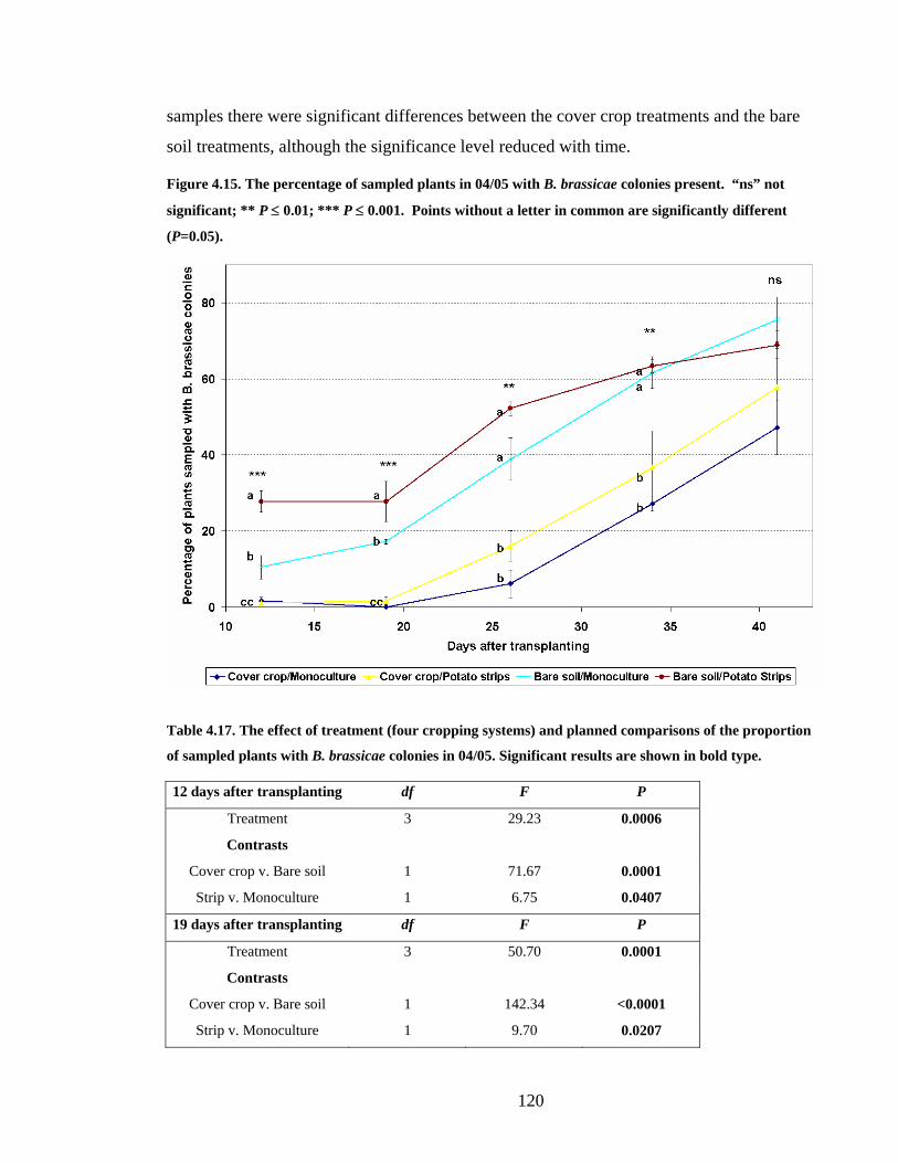
120
samples there were significant differences between the cover crop treatments and the bare
soil treatments, although the significance level reduced with time.
Figure 4.15. The percentage of sampled plants in 04/05 with B. brassicae colonies present. “ns” not
significant; ** P ≤ 0.01; *** P ≤ 0.001. Points without a letter in common are significantly different
(P=0.05).
Table 4.17. The effect of treatment (four cropping systems) and planned comparisons of the proportion
of sampled plants with B. brassicae colonies in 04/05. Significant results are shown in bold type.
12 days after transplanting df F P
Treatment 3 29.23 0.0006
Contrasts
Cover crop v. Bare soil 1 71.67 0.0001
Strip v. Monoculture 1 6.75 0.0407
19 days after transplanting df F P
Treatment 3 50.70 0.0001
Contrasts
Cover crop v. Bare soil 1 142.34 <0.0001
Strip v. Monoculture 1 9.70 0.0207
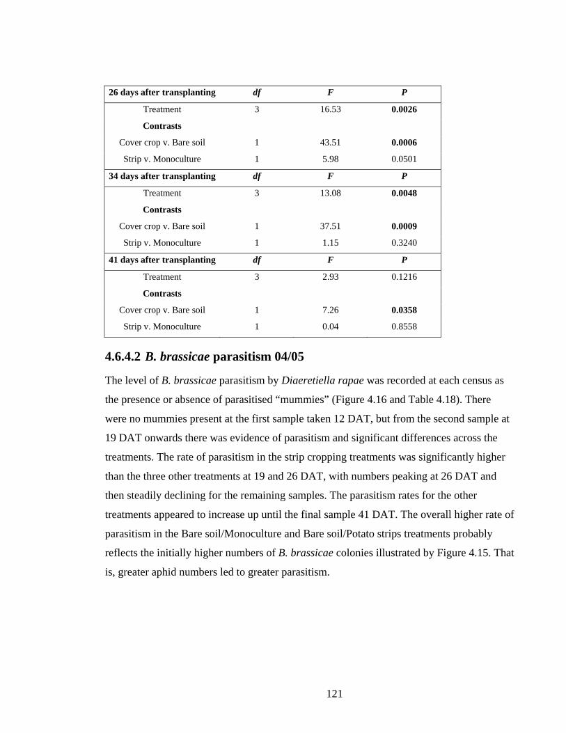
121
26 days after transplanting df F P
Treatment 3 16.53 0.0026
Contrasts
Cover crop v. Bare soil 1 43.51 0.0006
Strip v. Monoculture 1 5.98 0.0501
34 days after transplanting df F P
Treatment 3 13.08 0.0048
Contrasts
Cover crop v. Bare soil 1 37.51 0.0009
Strip v. Monoculture 1 1.15 0.3240
41 days after transplanting df F P
Treatment 3 2.93 0.1216
Contrasts
Cover crop v. Bare soil 1 7.26 0.0358
Strip v. Monoculture 1 0.04 0.8558
4.6.4.2 B. brassicae parasitism 04/05
The level of B. brassicae parasitism by Diaeretiella rapae was recorded at each census as
the presence or absence of parasitised “mummies” (Figure 4.16 and Table 4.18). There
were no mummies present at the first sample taken 12 DAT, but from the second sample at
19 DAT onwards there was evidence of parasitism and significant differences across the
treatments. The rate of parasitism in the strip cropping treatments was significantly higher
than the three other treatments at 19 and 26 DAT, with numbers peaking at 26 DAT and
then steadily declining for the remaining samples. The parasitism rates for the other
treatments appeared to increase up until the final sample 41 DAT. The overall higher rate of
parasitism in the Bare soil/Monoculture and Bare soil/Potato strips treatments probably
reflects the initially higher numbers of B. brassicae colonies illustrated by Figure 4.15. That
is, greater aphid numbers led to greater parasitism.
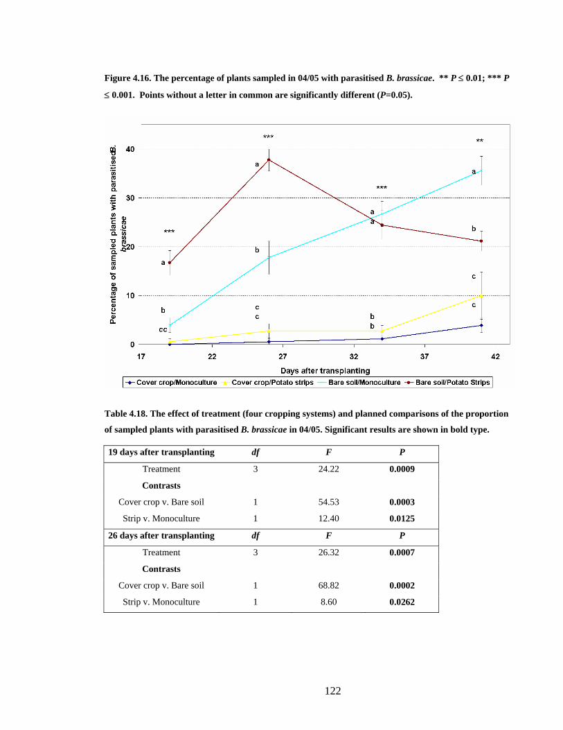
122
Figure 4.16. The percentage of plants sampled in 04/05 with parasitised B. brassicae. ** P ≤ 0.01; *** P
≤ 0.001. Points without a letter in common are significantly different (P=0.05).
Table 4.18. The effect of treatment (four cropping systems) and planned comparisons of the proportion
of sampled plants with parasitised B. brassicae in 04/05. Significant results are shown in bold type.
19 days after transplanting df F P
Treatment 3 24.22 0.0009
Contrasts
Cover crop v. Bare soil 1 54.53 0.0003
Strip v. Monoculture 1 12.40 0.0125
26 days after transplanting df F P
Treatment 3 26.32 0.0007
Contrasts
Cover crop v. Bare soil 1 68.82 0.0002
Strip v. Monoculture 1 8.60 0.0262

123
34 days after transplanting df F P
Treatment 3 34.73 0.0003
Contrasts
Cover crop v. Bare soil 1 102.23 <0.0001
Strip v. Monoculture 1 0.38 0.5610
41 days after transplanting df F P
Treatment 3 14.63 0.0036
Contrasts
Cover crop v. Bare soil 1 36.84 0.0009
Strip v. Monoculture 1 0.29 0.6114
4.6.4.3 B. brassicae colonies 05/06
There were significant treatment differences in the number of alate B. brassicae recorded in
all four samples in 05/06 (Figure 4.17). Like the P. xylostella data from 05/06, the number
of alate B. brassicae were significantly higher in the bare soil treatments compared to the
cover crop treatments, although there was some treatment overlap at 29 and 36 DAT
indicated by the LSD’s. When these results were analysed using pairwise contrasts there
were very significant differences with greater numbers of alate B. brassicae in bare soil
treatments compared to cover crop treatments (Table 4.19). This indicates that B. brassicae
was less effective at colonising broccoli planted in a cover crop compared to bare soil.

124
Figure 4.17. The mean number of alate B. brassicae per plant sampled in 05/06. ** P ≤ 0.01; *** P ≤
0.001. Points without a letter in common are significantly different (P=0.05).
Table 4.19. The effect of treatment (six cropping systems) and planned comparisons of the abundance
of alate B. brassicae in 05/06. Significant results are shown in bold type.
14 days after transplanting df F P
Treatment 5 53.17 <0.0001
Contrasts
Cover crop v. Bare soil 1 254.56 <0.0001
Strip v. Monoculture 1 0.93 0.3473
Bare soil strip v. Bare soil monoculture 1 0.83 0.3730
22 days after transplanting df F P
Treatment 5 15.12 <0.0001
Contrasts
Cover crop v. Bare soil 1 69.98 <0.0001
Strip v. Monoculture 1 0.08 0.7844
Bare soil strip v. Bare soil monoculture 1 0.15 0.6991
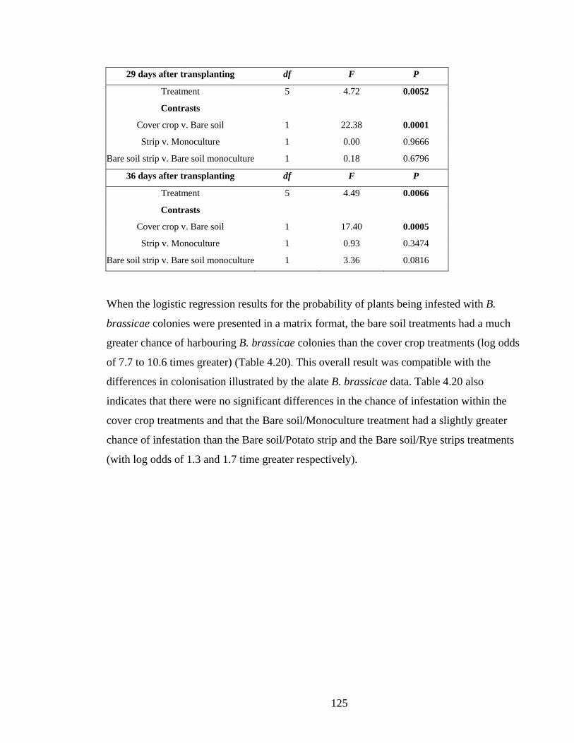
125
29 days after transplanting df F P
Treatment 5 4.72 0.0052
Contrasts
Cover crop v. Bare soil 1 22.38 0.0001
Strip v. Monoculture 1 0.00 0.9666
Bare soil strip v. Bare soil monoculture 1 0.18 0.6796
36 days after transplanting df F P
Treatment 5 4.49 0.0066
Contrasts
Cover crop v. Bare soil 1 17.40 0.0005
Strip v. Monoculture 1 0.93 0.3474
Bare soil strip v. Bare soil monoculture 1 3.36 0.0816
When the logistic regression results for the probability of plants being infested with B.
brassicae colonies were presented in a matrix format, the bare soil treatments had a much
greater chance of harbouring B. brassicae colonies than the cover crop treatments (log odds
of 7.7 to 10.6 times greater) (Table 4.20). This overall result was compatible with the
differences in colonisation illustrated by the alate B. brassicae data. Table 4.20 also
indicates that there were no significant differences in the chance of infestation within the
cover crop treatments and that the Bare soil/Monoculture treatment had a slightly greater
chance of infestation than the Bare soil/Potato strip and the Bare soil/Rye strips treatments
(with log odds of 1.3 and 1.7 time greater respectively).

126
Table 4.20. B. brassicae colonies in 05/06 logistic regression estimates with P values in brackets.
Significant tests are shown in bold type.
Cover crop
Monoculture
Cover crop
Rye Strips
Cover crop
Potato strips
Bare soil
Monoculture
Bare soil
Rye strips
Cover crop
Rye strips
0.56
(P=0.3298)
Cover crop
Potato strips
-0.62
(P=0.3379)
-1.17
(P=0.0586)
Bare soil
Monoculture
10.04
(P<0.0001)
10.66
(P<0.0001)
9.48
(P<0.0001)
Bare Soil
Rye strips
8.33
(P<0.0001)
8.95
(P<0.0001)
7.77
(P<0.0001)
-1.71
(P=0.0054)
Bare soil
Potato strips
8.70
(P<0.0001)
9.32
(P<0.0001)
8.14
(P<0.0001)
-1.34
(P=0.0299)
0.3703
(P=0.4549)
When the probability of aphids being present in each individual treatment was expressed
graphically with the inclusion of 95% confidence intervals, it was evident that there was a
very low probability of B. brassicae infestation in the cover crop treatments (Figure 4.18).
Furthermore, the Bare soil/Potato strips and the Bare soil/Rye strips treatments had a lower
probability of infestation than the Bare soil/Monoculture. This provides evidence that the
cover crop and possibly the level of field fragmentation had a significant negative effect on
the number of B. brassicae colonies in cropping systems.

127
Figure 4.18. The probability of B. brassicae presence on broccoli plants with 95% confidence intervals.
4.6.4.4 B. brassicae parasitism 05/06 Analysis of the B. brassicae parasitism data detected quasi-complete separation on some
blocking variables. This occurs when the outcome variable is almost completely explained
by the explanatory variables. Since this can result in unstable estimates these variables were
removed and the analysis repeated. This means that the latin square design (Block and
Row) and the sampling date (Replication) were not taken into account in the model. Using
this process the variation that was explained by the blocking variables was now explained
by the treatments alone, which resulted in large variations. However, the same trends
identified in the B. brassicae colonies data from 05/06 were present in the logistic
regression matrix of B. brassicae parasitism, except that the regression estimates were
lower (Table 4.21).

128
Table 4.21. B. brassicae parasitism in 05/06 logistic regression estimates with P values in brackets.
Significant tests are in bold type.
Cover crop
Monoculture
Cover crop
Rye Strips
Cover crop
Potato strips
Bare soil
Monoculture
Bare soil
Rye strips
Cover crop
Rye strips
0.81
(P=0.0648)
Cover crop
Potato strips
1.01
(P=0.0193)
0.20
(P=0.5876)
Bare soil
Monoculture
3.81
(P<0.0001)
3.00
(P<0.0001)
2.80
(P<0.0001)
Bare Soil
Rye strips
2.74
(P<0.0001)
1.93
(P<0.0001)
1.73
(P<0.0001)
-1.06
(P=0.0030)
Bare soil
Potato strips
3.39
(P<0.0001)
2.58
(P<0.0001)
2.38
(P<0.0001)
-0.42
(P<0.0001)
0.64
(P=0.0525)
When the probability of aphids being parasitised in each individual treatment was
expressed graphically with the inclusion of 95% confidence intervals, large variations
caused by the removal of blocking variables were evident (Figure 4.19). However, there
appears to be a greater probability of finding evidence of parasitism (mummies) in the
cover crop treatments than finding live colonies in the cover crops, especially in the Cover
crop/Potato strips and the Cover crop/Rye strips treatments. The results from the bare soil
treatments are an approximation of the B. brassicae colonies data except that the
probability of parasitism was generally higher. This indicates that there was a greater
probability of finding parasitised aphids in the bare soil treatments than live colonies.
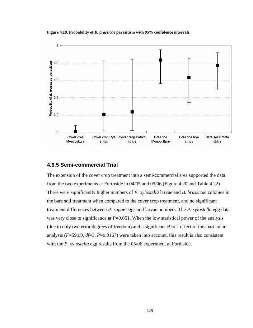
129
Figure 4.19. Probability of B. brassicae parasitism with 95% confidence intervals.
4.6.5 Semi-commercial Trial
The extension of the cover crop treatment into a semi-commercial area supported the data
from the two experiments at Forthside in 04/05 and 05/06 (Figure 4.20 and Table 4.22).
There were significantly higher numbers of P. xylostella larvae and B. brassicae colonies in
the bare soil treatment when compared to the cover crop treatment, and no significant
treatment differences between P. rapae eggs and larvae numbers. The P. xylostella egg data
was very close to significance at P=0.051. When the low statistical power of the analysis
(due to only two error degrees of freedom) and a significant Block effect of this particular
analysis (F=59.00, df=3, P=0.0167) were taken into account, this result is also consistent
with the P. xylostella egg results from the 05/06 experiment at Forthside.
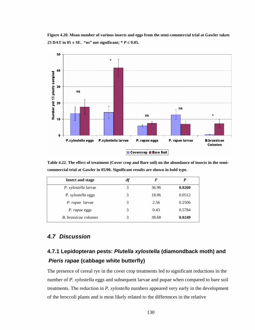
130
Figure 4.20. Mean number of various insects and eggs from the semi-commercial trial at Gawler taken
23 DAT in 05 ± SE. “ns” not significant; * P ≤ 0.05.
Table 4.22. The effect of treatment (Cover crop and Bare soil) on the abundance of insects in the semi-
commercial trial at Gawler in 05/06. Significant results are shown in bold type.
Insect and stage df F P
P. xylostella larvae 3 36.96 0.0260
P. xylostella eggs 3 18.06 0.0512
P. rapae larvae 3 2.56 0.2506
P. rapae eggs 3 0.43 0.5784
B. brassicae colonies 3 38.68 0.0249
4.7 Discussion
4.7.1 Lepidopteran pests: Plutella xylostella (diamondback moth) and Pieris rapae (cabbage white butterfly)
The presence of cereal rye in the cover crop treatments led to significant reductions in the
number of P. xylostella eggs and subsequent larvae and pupae when compared to bare soil
treatments. The reduction in P. xylostella numbers appeared very early in the development
of the broccoli plants and is most likely related to the differences in the relative
131
distributions of P. xylostella eggs oviposited across the treatments. There were slight
reductions in the number of P. xylostella larvae when the strip cropping treatments were
compared to the Bare soil/Monoculture (conventional practice) at 22, 36 and 44 DAT in the
05/06 experiment, but these differences were not consistent across years and were minimal
in comparison to the differences between the cover crop treatments and the bare soil
treatments. In comparison to P. xylostella, the numbers of P. rapae eggs and larvae were
relatively consistent across the treatments, which resulted in a more even distribution of P.
rapae larvae and very few significant differences between treatments. The distinct
differences between the relative numbers of eggs and larvae of both P. xylostella and P.
rapae in cover crops and bare soil treatments was further supported by data from the semi-
commercial trial.
If the reduced number of P. xylostella eggs in the cover crop treatments were due to egg
predation (in line with the “enemies hypothesis” of Root [1973]) then it would be expected
that the same effect would also be acting on the P. rapae egg numbers, as they are known
to suffer high levels of egg predation (Schmaedick and Shelton 1999). Although predation
of P. rapae eggs was not assessed, P. xylostella egg predation was, and unlike the P.
xylostella egg data collected from the destructive samples, there were no distinct
differences between the cover crop and bare soil treatments. These two pieces of
information suggest that the low number of P. xylostella eggs in the cover crop treatments
was due to fewer eggs being oviposited.
There is other evidence that P. xylostella oviposition can be negatively affected by cover
crops, as previous research on other Brassica crops and cereal cover crop mixtures by
Bukovinszky et al. (2004) found that number of both P. xylostella larvae and pupae were
significantly reduced in barley-brussels sprouts intercrops. Mangan et al. (1995) and Mwaja
et al. (1996) found fewer P. xylostella larvae on cabbages grown with cover crops,
including cereal rye, when compared to conventional tillage. Bukovinszky et al. (2005)
suggested that a barley background decreased the linear dimensions of plant patches so that
plants no longer “loomed up” from the background, hence altering the perception of
dimensional visual and olfactory cues. Furthermore, greater complexity with an extra

132
vegetational background in the cover cropping treatments might have made the P.
xylostella lose host plants (Bukovinszky et al. 2005) or caused insects to alight
“inappropriately” (Finch and Collier 2000) interfering with host location or host
acceptance. The experiments detailed in this chapter cannot determine if the reductions in
P. xylostella egg numbers were due to host location difficulties or reductions in oviposition
due to interference with host acceptance behaviour. However, the most likely cause is
interference with host location, as Finch and Collier (2000) suggest that P. xylostella adult
females do not require much stimulus to oviposit and are likely to lay an egg on the first
host plant encountered.
Replacing dead rye with living cover crops (that is, living mulches) may not necessarily
lead to a reduction in P. xylostella numbers. Finch and Kienegger (1997) showed in a study
of eight Brassica pest species (including P. rapae) that P. xylostella was affected the least
by live clover backgrounds. This is supported by the experiment in 04/05 where an attempt
was made to mimic a living mulch by painting the dead rye cover crop green but this did
not result in any significant differences in insect numbers.
Another possible explanation of the reduction in P. xylostella numbers is that the cover
crop caused a decline in crop growth and hence host plant attractiveness (Theunissen 1994),
as plants in the cover crop treatments were slower growing and therefore smaller at any
given time (Chapter 5). Conversely, P. rapae have a limited ability to discern host plant
quality as they will oviposit on plants already laden with eggs and larvae, or plants that are
stunted or have lower concentrations of nitrogen (Root and Kareiva 1984). However,
results from trap crop choice tests show that leaf area, leaf shape and plant architecture
appear not to be major factors in determining P. xylostella oviposition preferences
(Badenes-Perez et al. 2004). Furthermore the oviposition leaf choice tests performed in the
adult moth cage in the glasshouse did not provide any evidence of oviposition preferences
across the treatments.
Another factor could be the sulphur content of the plants as the sap tests performed on the
different treatments indicated that there was less sulphur in the cover crop broccoli plants

133
(Chapter 5), which has been shown to reduce P. xylostella oviposition (Marazzi et al. 2004;
Marazzi and Stadler 2004). However, these published experiments compared the extreme
situation of plants grown without sulphur to normally fertilised plants or plants with excess
sulphur nutrition and are not supported by results from the laboratory population
oviposition experiment. Experiments have also shown that different sulphur fertilisation
rates have no significant effect on glucosinolate concentrations in broccoli inflorescences
(Vallejo et al. 2003) and that glucosinolates are the stimulus for oviposition in P. xylostella
(Reed et al. 1989).
The P. rapae results obtained from the 04/05 and 05/06 experiments are in agreement with
Masiunas et al. (1997) who found no significant difference in the presence of P. rapae
when comparing cabbages grown using conventional tillage (bare soil) or cereal rye cover
crops. In general, P. rapae are reported to have the ability to precisely identify cruciferous
plants (Root and Kareiva 1984) and are not affected by scales of landscape fragmentation
(Banks 1998) or intercropping (Theunissen and den Ouden 1980). Unlike other
Lepidopteran pests such as P. xylostella, P. rapae have been shown to have a significant
negative relationship between plot size and the number of eggs laid per plant (Cromartie
1975; Bukovinszky et al. 2005), regardless of plant size, time of year or background
(Cromartie 1975). Possibly due to host plant deprivation leading to gravid P. rapae females
having higher motivation to oviposit more eggs on each plant successfully located in a
patchy environment (Hern et al. 1996). Root and Kareiva (1984) describe the ovipositing
behaviour of P. rapae as a Markovian process, which leads to an almost random spread of
eggs on plants in a wide area. Root and Kareiva (1984) theorised that the egg spreading
behaviour of an adult P. rapae female is an adaptive response that spreads the risk of her
offspring’s deaths among several plants. Furthermore, P. rapae butterflies in Australia have
been found to spread their eggs more widely than P. rapae butterflies in Canada and the
UK (Hern et al. 1996). All these factors lead to cover crops being an ineffective strategy in
the control of P. rapae. This finding does not support assertions made by Potting et al.
(2005) who expected that diversification strategies would be more effective on more highly
mobile insect herbivores with directed flights and good sensory abilities that enable
134
oriented movements. However, these assertions were based on simulations and not field
experiments.
Strip cropping dispersed two rows of broccoli plants amongst rows of potatoes (Potato
strips treatments in 04/05 and 05/06) or standing rye (Rye strips treatment in 05/06), which
in effect reduced the patch size of the broccoli stands. This field fragmentation had no
significant affect on the number of P. xylostella larvae and pupae or P. rapae larvae. The P.
xylostella results are in agreement with Bukovinszky et al. (2005) who found that P.
xylostella larvae and pupae numbers were not affected by patch size. In the case of P.
rapae, the failure of strip cropping could be related to greater perimeter to area ratios
compared to the monocultures, meaning that P. rapae were more likely to “find” strips
though increased encounter rates (Bukovinszky et al. 2005). This theory agrees with Root
(1973) who found that on 88% of sampling occasions P. rapae abundance was greater in
perimeter rows than in pure stands and only during population peaks was abundance higher
in the pure stands compared to the perimeter rows.
There is no evidence that potatoes are an alternative host to the members of the Brassica
pest complex. Therefore, broccoli strip cropping might be a more successful practice in the
reduction of insect pests, if potatoes were replaced with a trap crop that is more attractive to
insect pests either preventing them from reaching the crop, or concentrating them in an area
where they can be chemically controlled (Hokkanen 1991). Alternatively, yellow rocket
(Barbarea vulgaris var. arcuata) may provide a more attractive alternative host to the pest,
and has the added benefit of not sustaining the development of P. xylostella larvae
(Badenes-Perez et al. 2004). However, caution must be applied as not all purported trap
crops are consistently effective. In a study of cabbage plots with Indian mustard (Brassica
juncea) borders as trap crops by Luther et al. (1996) found no statistical differences in the
presence of P. xylostella larvae or pupae. Another factor to consider is the economics of
trap cropping, as replacing a percentage of a commercial crop with a trap crop might be
appropriate from an insect control perspective but may not be financially viable.
135
4.7.2 Breviocoryne brassicae (cabbage aphid)
In all the experiments, including the semi-commercial trial, there were significantly fewer
B. brassicae in the cover crop treatments than the bare soil treatments. Lower numbers of
B. brassicae in cover crops and living mulches has been previously described (Tukahirwa
and Coaker 1982; Costello 1994; Costello 1995; Theunissen et al. 1995; Vidal 1997).
Aphids are known to locate plants using the contrast between the plant and the soil
background to guide them (Doring et al. 2004). The cover crop could have acted as an
optical competitor reducing the contrast between the background and the green host plant
inducing an “inappropriate” landing (Finch and Collier 2000) on the cereal rye.
Furthermore, upon alighting on a cover crop, the surface encourages probing activity that in
turn induces a host rejection response (Doring et al. 2004), which induces the insect to
leave the patch in much the same fashion as Finch and Collier (2000)’s
appropriate/inappropriate landing theory. Alighting on soil does not induce probing and the
aphid will walk or fly towards a green target (Doring et al. 2004). However, cover crops
only appear to be an effective strategy when the background vegetation is dense compared
to the host plant (Theunissen and den Ouden 1980; Tukahirwa and Coaker 1982), which
can help to explain the observed increase in the number of alate B. brassicae and colonies
over time. As the broccoli plants grew they occupied a greater area and thus reduced the
contrast between the cover crop background and the broccoli plants. This in turn could have
increased the colonisation rates of alate B. brassicae from outside the trial area by
improving the likelihood of an “appropriate” landing on the host plant (Finch and Collier
2000). Another explanation for the increase in the numbers of aphids in the cover cropping
treatments might simply be the ability of a few B. brassicae colonisers to rapidly increase
numbers by producing fast developing live young from unfertilised eggs.
In the 04/05 experiment, there were initially more aphid colonies in the Bare soil/Potato
strips treatment than the monoculture treatment. The same trend was also evident in the
colonisation rates by alate B. brassicae in the 05/06 experiment, indicating that when the
broccoli plants are small, the potato strips may orient flying alate aphids along these rows
making them more likely to locate broccoli plants in between potato plants. However,
analysis of the aphid colony distribution in 05/06 showed that B. brassicae numbers were
136
likely to be higher in the Bare soil/Monoculture than both the bare soil strip cropping
treatments. These conflicting results can also be found in other published studies.
Bukovinszky et al. (2005) found that B. brassicae densities were independent of patch size
due to them being contact searchers with low maximum flight speeds and a strong
arrestment response, making them unlikely to actively travel once a host plant is located.
Banks (1998) found that all tested scales of landscape fragmentation negatively affected B.
brassicae densities. Potting et al. (2005) agrees with Bukovinszky et al. (2005), finding that
in simulations very small alate insects (like aphids) would be the most difficult pests to
control with a diversification strategy as they have an airborne colonisation pattern, limited
host detection ability and slow displacement speed. However, results from both
Bukovinszky et al. (2005) and Potting et al. (2005) do not explain the observed differences
between the cover crop and bare soil treatments as colonisation by chance alone should
result in the consistent colonisation trends of treatment groups reported here.
4.7.3 Parasitism Rates
There were no significant differences in the parasitism rates of P. xylostella in 04/05 or
05/06. The pupal data from 05/06 showed that every P. xylostella pupae collected was
parasitised. The data did not indicate that parasitoids in the experiment were less able to
locate their target species in mixed cropping situations where there are also fewer
individuals. This agrees with Bukovinszky et al. (2005) who found that parasitism rates of
P. xylostella by Diadegma spp. were not affected by patch size or vegetation background.
Complete parasitism of pupae in 05/06 could possibly explain the reduction in adult moth
numbers over the course of the experiment as each parasitised P. xylostella larva or pupa
results in the recruitment of a parasitic wasp into the next generation and not a moth. This
directly reduces moth numbers and increases parasitism (Hamilton et al. 2004).
These high rates of parasitism can have major implications to the number of P. xylostella in
a cropping system, as they have a relatively short life cycle, which under Australian
conditions leads to a number of generations per season (Mo et al. 2003).
In both the 04/05 and the 05/06 experiment B. brassicae parasitism rates by Diaeretiella
rapae appeared to be related to the relative numbers present in each treatment, rather than

137
the presence or absence of a cover crop. This finding is in agreement with Bukovinszky et
al. (2005) who found that vegetational background did not influence parasitism of B.
brassicae. Vidal (1997) found that parasitism of B. brassicae by D. rapae was only slightly
decreased by intercropping with rye grass (Lolium perenne). Results from experiments with
the green peach aphid (Myzus persicae) found no significant difference between
conventional tillage (bare soil) and cereal rye cover crops (Masiunas et al. 1997), while
Bukovinszky et al. (2004) found that the presence of natural enemies did not contribute to
differences in B. brassicae densities in Brussels sprouts intercropped with barley (Hordeum
vulgare).
4.8 Conclusions
The reduction in the number of P. xylostella and B. brassicae in the cover crop treatments
support the assertion that a reduction in contrast provided by the cover crop background
vegetation caused more of the landings to be “inappropriate” (Finch and Collier 2000)
resulting in insects losing the target plants or interfering with host acceptance behaviour
(Bukovinszky et al. 2005). Therefore lower densities of eggs, larvae and pupae of P.
xylostella and alate B. brassicae and B. brassicae colonies in the rye cover crop treatment
compared to the other treatments were most likely due to a different rate of colonisation
(Finch and Kienegger 1997) and not parasitism or predation.
A possible evolutionary mechanism for the P. xylostella and B. brassicae results could be
the co-development of the plants and their pest complexes as Brassicas developed in a
niche provided by unstable land surfaces and are accustomed to growing in bare broken
ground. Therefore, insect pests of Brassica crops would also presumably be adapted to
finding plants in bare ground situations and not amongst background vegetation (Kostal and
Finch 1994) including cover crops. However, this theory does not account for the behaviour
of P. rapae, which was presumably also exposed to the same evolutionary mechanisms and
yet the results presented here illustrate that the cover crop had no significant effect.
All the insect data indicated that there were no significant pest control benefits that could
be derived from strip cropping. This is in spite of strip cropping Brassica plants with non-

138
host plants increasing the “clumpiness” of vegetation and fragmentation (Hern et al. 1996).
This suggests that host plant location is not influenced by the presence of potatoes or the
patchiness of the strip cropping treatments when compared to the monoculture treatments.
These results suggest that insect plant discrimination operates at a smaller scale than a
1.65m strip, which contradicts the notions that mixed species cropping strategies,
particularly strip cropping, could be important pest management tools in sustainable
cropping systems (Rämert 2002).
Another factor to take into account when discussing the impact of plant diversity on
herbivore behaviour, or making recommendations, is the need to clearly distinguish
between different insects as to how active and perceptive they are (Banks and Ekbom
1999). P. rapae, with its highly developed visual and olfactory host location ability (Banks
1998), large size, daytime activity, Markovian movements (Root and Kareiva 1984) and
very active egg spreading behaviour (Cromartie 1975; Root and Kareiva 1984; Hern et al.
1996; Bukovinszky et al. 2005) is not affected by increased plant species diversity in the
cropping system. However, P. rapae are not a significant pest in Australia and relative to P.
xylostella they are easier to control using insecticides.

139
Chapter 5 The impacts of a rye cover crop and strip crops on yield and quality of potatoes and broccoli
5.1 Introduction
The previous chapter demonstrated that a rye cover crop could result in significant
reductions in the number of two commercially important pests in Australia. This chapter
explores the agronomic effects of the rye cover crop and strip cropping on crop growth,
yield, quality and gross margins from experiments conducted in the summers of 04/05 and
05/06.
5.2 Methodology
The experimental designs, sampling structures and planned contrasts of the analysis
described in this chapter are the same as those described in Chapter 4. To avoid repetition
only the methods that are specific to this chapter will be detailed.
5.2.1 Potato cover crop treatment planting and management 04/05
The establishment of the potato cover crop treatments in 04/05 differs from that of the other
potato treatments discussed in Chapter 4. The potato cover crop treatments were pre-
moulded into two ridges per 1.65m bed on 7 September 04. Cereal rye was then hand
broadcast onto the moulds at the same rate as the broccoli cover crop treatments, with
100kg/ha of seed and 50kg/ha of fertiliser (14N:16P:11K). The moulds were then hand
raked to cover the seed. The potatoes in the cover crop treatments were planted into the
standing rye on 4 November 04, on the same day as potatoes in the other treatments using
the same equipment. The planting process significantly suppressed the cover crop (Picture
5.1). On 2 December the cover crop was killed and weeds were controlled in all potato
treatments with an application of Sprayseed® (paraquat 0.189kg a.i./ha and diquat 0.161kg
ai/ha).

140
Picture 5.1. Potato Cover crop/Monoculture after planting 04/05.
5.2.2 Potato yield and quality assessment 04/05
In the 04/05 experiment, all the potatoes from each plot, except the outermost plot edge
(guard) rows, were lifted to the surface with a twin row potato digger and bagged by hand
(Picture 5.2). Potato yields were assessed as entire plot yields. Two approximately 20kg
samples from each plot were graded for size and quality (as per Chapter 3). The quality
parameters included the weight ranges of 850g-250g tubers (Large); 250g-75g tubers
(Medium); and under 75g tubers (Small); as well as the percentage of tubers meeting the
‘Bonus’ category for both size and quality (for example free of bruising); and the total
potatoes rejected for defects (Rejects).
Picture 5.2. Digging (left) and bagging (right) potatoes from the 04/05 experiment.
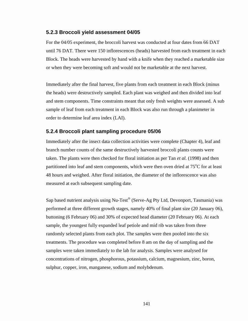
141
5.2.3 Broccoli yield assessment 04/05
For the 04/05 experiment, the broccoli harvest was conducted at four dates from 66 DAT
until 76 DAT. There were 150 inflorescences (heads) harvested from each treatment in each
Block. The heads were harvested by hand with a knife when they reached a marketable size
or when they were becoming soft and would not be marketable at the next harvest.
Immediately after the final harvest, five plants from each treatment in each Block (minus
the heads) were destructively sampled. Each plant was weighed and then divided into leaf
and stem components. Time constraints meant that only fresh weights were assessed. A sub
sample of leaf from each treatment in each Block was also run through a planimeter in
order to determine leaf area index (LAI).
5.2.4 Broccoli plant sampling procedure 05/06
Immediately after the insect data collection activities were complete (Chapter 4), leaf and
branch number counts of the same destructively harvested broccoli plants counts were
taken. The plants were then checked for floral initiation as per Tan et al. (1998) and then
partitioned into leaf and stem components, which were then oven dried at 75oC for at least
48 hours and weighed. After floral initiation, the diameter of the inflorescence was also
measured at each subsequent sampling date.
Sap based nutrient analysis using Nu-Test® (Serve-Ag Pty Ltd, Devonport, Tasmania) was
performed at three different growth stages, namely 40% of final plant size (20 January 06),
buttoning (6 February 06) and 30% of expected head diameter (20 February 06). At each
sample, the youngest fully expanded leaf petiole and mid rib was taken from three
randomly selected plants from each plot. The samples were then pooled into the six
treatments. The procedure was completed before 8 am on the day of sampling and the
samples were taken immediately to the lab for analysis. Samples were analysed for
concentrations of nitrogen, phosphorous, potassium, calcium, magnesium, zinc, boron,
sulphur, copper, iron, manganese, sodium and molybdenum.
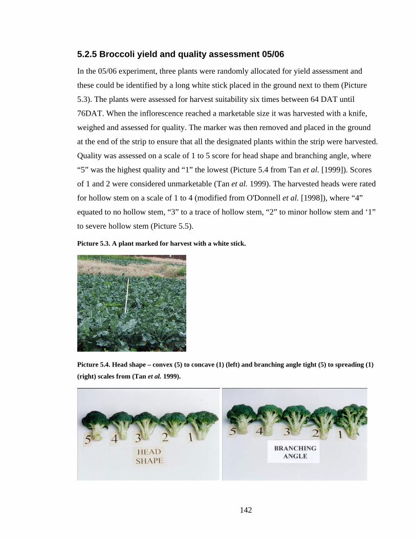
142
5.2.5 Broccoli yield and quality assessment 05/06
In the 05/06 experiment, three plants were randomly allocated for yield assessment and
these could be identified by a long white stick placed in the ground next to them (Picture
5.3). The plants were assessed for harvest suitability six times between 64 DAT until
76DAT. When the inflorescence reached a marketable size it was harvested with a knife,
weighed and assessed for quality. The marker was then removed and placed in the ground
at the end of the strip to ensure that all the designated plants within the strip were harvested.
Quality was assessed on a scale of 1 to 5 score for head shape and branching angle, where
“5” was the highest quality and “1” the lowest (Picture 5.4 from Tan et al. [1999]). Scores
of 1 and 2 were considered unmarketable (Tan et al. 1999). The harvested heads were rated
for hollow stem on a scale of 1 to 4 (modified from O'Donnell et al. [1998]), where “4”
equated to no hollow stem, “3” to a trace of hollow stem, “2” to minor hollow stem and ‘1”
to severe hollow stem (Picture 5.5).
Picture 5.3. A plant marked for harvest with a white stick.
Picture 5.4. Head shape – convex (5) to concave (1) (left) and branching angle tight (5) to spreading (1)
(right) scales from (Tan et al. 1999).

143
Picture 5.5. Broccoli hollow stem scale with rankings in brackets (from left) – no hollow stem (4), trace
(3), minor (2) and severe (1).
5.2.6 Data analysis 04/05 and 05/06
The potato and broccoli data from the 04/05 and the 05/06 experiments were analysed using
one way ANOVA’s in the same manner as the P. xylostella and P. rapae insect data, as
discussed in Chapter 4.
5.3 Results
5.3.1 Potato yields 04/05
Potato yields were not significantly different across the four treatments (F=0.01, df=3,
p=0.9561) and there was little variation between the plots (Table 5.1).
Table 5.1. Potato treatment yields 04/05.
Treatment Number
(n)
Mean weight per
plot (kg) ± SE
Cover crop/Monoculture 3 386.87 ± 17.60
Cover crop/Broccoli strips 3 388.37 ± 12.56
Tilled soil/Monoculture 3 384.25 ± 3.56
Tilled soil/Broccoli strips 3 394.48 ± 12.73
When the harvested potatoes were assessed for quality, according to commercial
specifications, the results were also not significant (Figure 5.1 and Table 5.2).

144
Figure 5.1. The percentage by weight of the 04/05 potato harvest allocated to each quality category ± SE
Table 5.2. The effect of treatment (four cropping systems) and planned comparisons of potato yield and
quality in 04/05.
Total yield df F P
Treatment 3 0.10 0.9561
Contrasts
Cover crop v. Bare soil 1 0.02 0.9019
Strip v. Monoculture 1 0.28 0.6143
Large tubers df F P
Treatment 3 0.21 0.8868
Contrasts
Cover crop v. Bare soil 1 0.00 0.9673
Strip v. Monoculture 1 0.01 0.9258
Medium tubers df F P
Treatment 3 0.16 0.9199
Contrasts
Cover crop v. Bare soil 1 0.00 0.9702
Strip v. Monoculture 1 0.01 0.9159
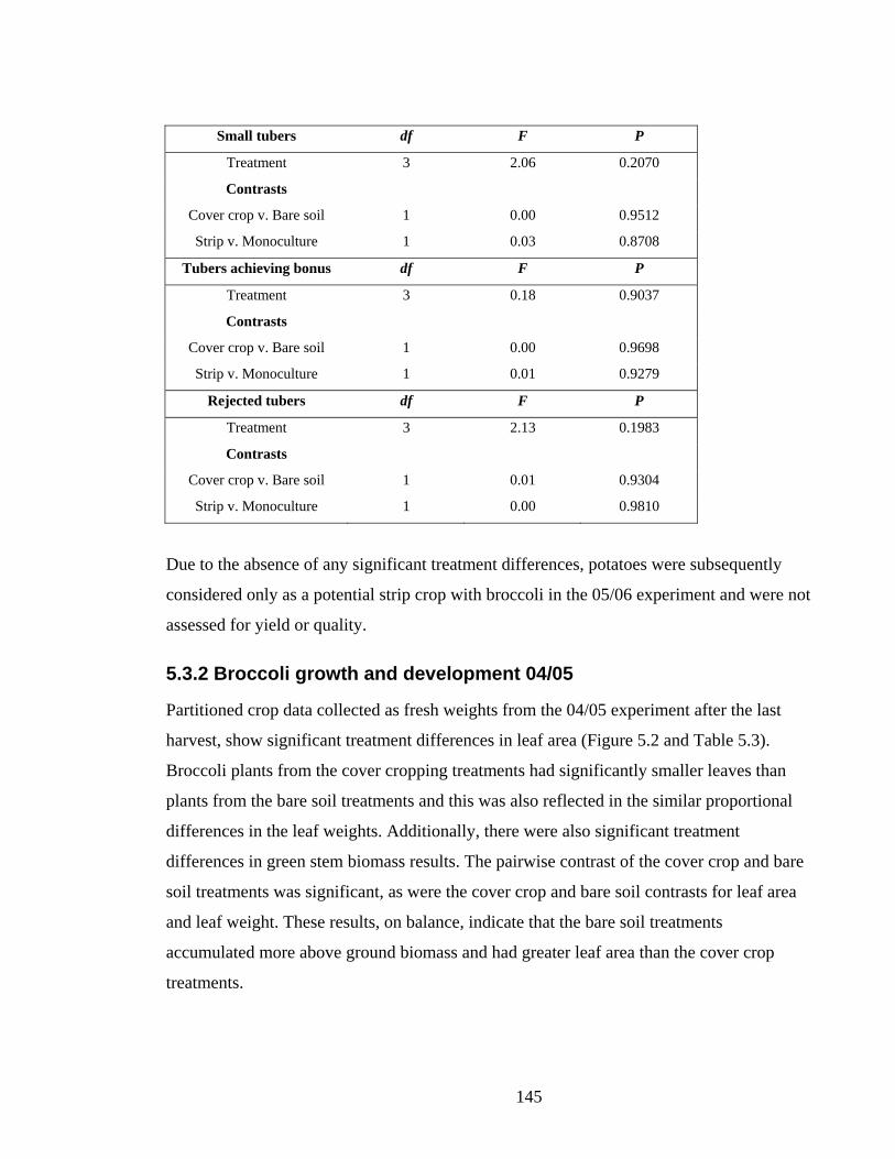
145
Small tubers df F P
Treatment 3 2.06 0.2070
Contrasts
Cover crop v. Bare soil 1 0.00 0.9512
Strip v. Monoculture 1 0.03 0.8708
Tubers achieving bonus df F P
Treatment 3 0.18 0.9037
Contrasts
Cover crop v. Bare soil 1 0.00 0.9698
Strip v. Monoculture 1 0.01 0.9279
Rejected tubers df F P
Treatment 3 2.13 0.1983
Contrasts
Cover crop v. Bare soil 1 0.01 0.9304
Strip v. Monoculture 1 0.00 0.9810
Due to the absence of any significant treatment differences, potatoes were subsequently
considered only as a potential strip crop with broccoli in the 05/06 experiment and were not
assessed for yield or quality.
5.3.2 Broccoli growth and development 04/05
Partitioned crop data collected as fresh weights from the 04/05 experiment after the last
harvest, show significant treatment differences in leaf area (Figure 5.2 and Table 5.3).
Broccoli plants from the cover cropping treatments had significantly smaller leaves than
plants from the bare soil treatments and this was also reflected in the similar proportional
differences in the leaf weights. Additionally, there were also significant treatment
differences in green stem biomass results. The pairwise contrast of the cover crop and bare
soil treatments was significant, as were the cover crop and bare soil contrasts for leaf area
and leaf weight. These results, on balance, indicate that the bare soil treatments
accumulated more above ground biomass and had greater leaf area than the cover crop
treatments.
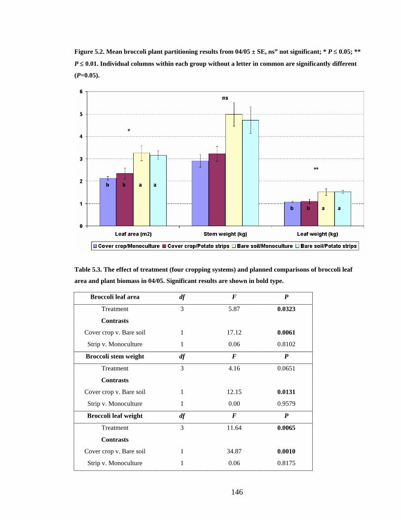
146
Figure 5.2. Mean broccoli plant partitioning results from 04/05 ± SE, ns” not significant; * P ≤ 0.05; **
P ≤ 0.01. Individual columns within each group without a letter in common are significantly different
(P=0.05).
Table 5.3. The effect of treatment (four cropping systems) and planned comparisons of broccoli leaf
area and plant biomass in 04/05. Significant results are shown in bold type.
Broccoli leaf area df F P
Treatment 3 5.87 0.0323
Contrasts
Cover crop v. Bare soil 1 17.12 0.0061
Strip v. Monoculture 1 0.06 0.8102
Broccoli stem weight df F P
Treatment 3 4.16 0.0651
Contrasts
Cover crop v. Bare soil 1 12.15 0.0131
Strip v. Monoculture 1 0.00 0.9579
Broccoli leaf weight df F P
Treatment 3 11.64 0.0065
Contrasts
Cover crop v. Bare soil 1 34.87 0.0010
Strip v. Monoculture 1 0.06 0.8175
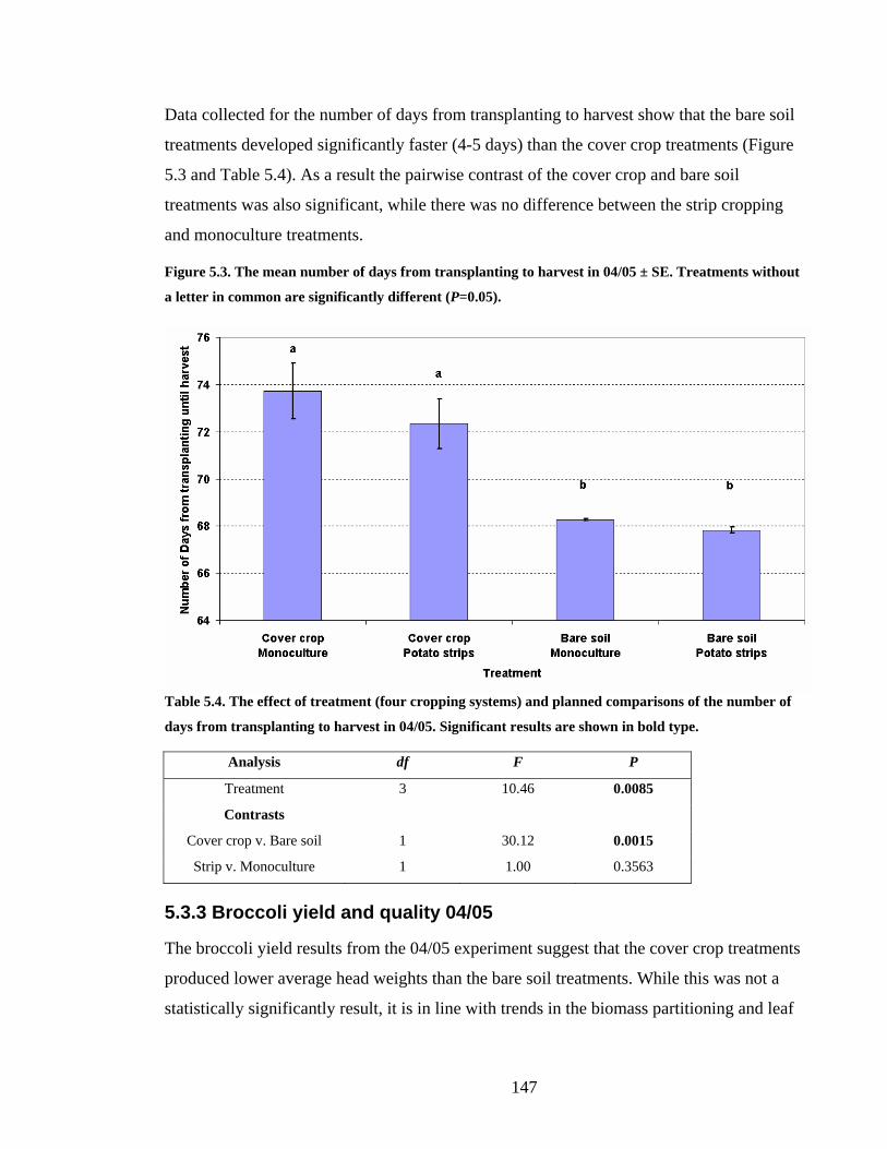
147
Data collected for the number of days from transplanting to harvest show that the bare soil
treatments developed significantly faster (4-5 days) than the cover crop treatments (Figure
5.3 and Table 5.4). As a result the pairwise contrast of the cover crop and bare soil
treatments was also significant, while there was no difference between the strip cropping
and monoculture treatments.
Figure 5.3. The mean number of days from transplanting to harvest in 04/05 ± SE. Treatments without
a letter in common are significantly different (P=0.05).
Table 5.4. The effect of treatment (four cropping systems) and planned comparisons of the number of
days from transplanting to harvest in 04/05. Significant results are shown in bold type.
Analysis df F P
Treatment 3 10.46 0.0085
Contrasts
Cover crop v. Bare soil 1 30.12 0.0015
Strip v. Monoculture 1 1.00 0.3563
5.3.3 Broccoli yield and quality 04/05
The broccoli yield results from the 04/05 experiment suggest that the cover crop treatments
produced lower average head weights than the bare soil treatments. While this was not a
statistically significantly result, it is in line with trends in the biomass partitioning and leaf

148
area results (Figure 5.4 and Table 5.5). The pairwise contrast of the cover crop treatments
and the bare soil treatments were also not significant.
Figure 5.4. Broccoli mean harvested head weights in 04/05 ± SE.
Table 5.5. The effect of treatment (four cropping systems) and planned comparisons of harvested head
weight per plant in 04/05. Significant results are shown in bold type.
df F P
Treatment 3 2.69 0.1398
Contrasts
Cover crop v. Bare soil 1 2.84 0.1429
Strip v. Monoculture 1 4.88 0.0692
The total accumulated yield for each plot indicates that there was significant variation
between the blocks, which reduced the likelihood of significant treatment differences
(Figure 5.5). The Cover crop/Monoculture treatment in Block 1 had a very low yield. This
was due to early establishment problems caused by a blocked sprinkler, resulting in only 70
harvestable heads of poor quality. Removing this data from the analysis did not result in a
statistically significant difference. Although not a significant result, the Bare soil/Potato
strips treatment had the greatest accumulated yield in each Block. Furthermore, the harvest
of the Bare soil/Potato strips treatment was completed in the fewest number of harvests

149
(two). This graph also indicates that the cover crop treatments were slower growing and
required more harvests than the bare soil treatments.
Figure 5.5. Total combined broccoli yields per plot in 04/05. DAT=days after transplanting.
5.3.4 Broccoli growth and development 05/06
Analysis of the mean number of leaves per plant in the 05/06 experiment showed that there
were very significant treatment differences at all but the first sampling date, with the bare
soil treatments having approximately twice the number of leaves as the cover crop
treatments (Figure 5.6 and Table 5.6). The pairwise contrasts of the cover crop and the bare
soil treatments were significant at every sampling date with the first sample having a lower
significance than the following six samples. The LSD’s for the treatments indicate that
there were no significant differences within the cover crop treatments from 22-59 DAT.
Within the bare soil treatments, the Bare soil/Monoculture treatment had significantly more
leaves than the other treatments at 36 and 52 DAT. However, at the final sample at 59 DAT
the Bare soil/Rye strips treatment had the greatest number of leaves.
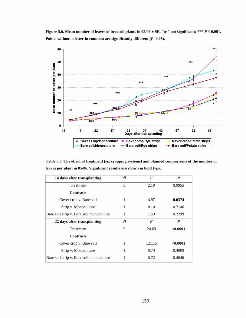
150
Figure 5.6. Mean number of leaves of broccoli plants in 05/06 ± SE. “ns” not significant; *** P ≤ 0.001.
Points without a letter in common are significantly different (P=0.05).
Table 5.6. The effect of treatment (six cropping systems) and planned comparisons of the number of
leaves per plant in 05/06. Significant results are shown in bold type.
14 days after transplanting df F P
Treatment 5 2.19 0.0955
Contrasts
Cover crop v. Bare soil 1 4.97 0.0374
Strip v. Monoculture 1 0.14 0.7146
Bare soil strip v. Bare soil monoculture 1 1.53 0.2299
22 days after transplanting df F P
Treatment 5 24.69 <0.0001
Contrasts
Cover crop v. Bare soil 1 121.15 <0.0001
Strip v. Monoculture 1 0.74 0.4000
Bare soil strip v. Bare soil monoculture 1 0.72 0.4046

151
29 days after transplanting df F P
Treatment 5 54.91 <0.0001
Contrasts
Cover crop v. Bare soil 1 271.12 <0.0001
Strip v. Monoculture 1 0.33 0.5739
Bare soil strip v. Bare soil monoculture 1 0.22 0.6448
36 days after transplanting df F P
Treatment 5 82.93 <0.0001
Contrasts
Cover crop v. Bare soil 1 383.96 <0.0001
Strip v. Monoculture 1 5.74 0.0265
Bare soil strip v. Bare soil monoculture 1 26.43 <0.0001
44 days after transplanting df F P
Treatment 5 112.10 <0.0001
Contrasts
Cover crop v. Bare soil 1 557.87 <0.0001
Strip v. Monoculture 1 0.73 0.4026
Bare soil strip v. Bare soil monoculture 1 0.41 0.5274
52 days after transplanting df F P
Treatment 5 68.98 <0.0001
Contrasts
Cover crop v. Bare soil 1 332.31 <0.0001
Strip v. Monoculture 1 1.92 0.1812
Bare soil strip v. Bare soil monoculture 1 6.37 0.0202
59 days after transplanting df F P
Treatment 5 19.39 <0.0001
Contrasts
Cover crop v. Bare soil 1 79.57 <0.0001
Strip v. Monoculture 1 1.23 0.2797
Bare soil strip v. Bare soil monoculture 1 0.36 0.5547
The greater number of leaves in the bare soil treatments also meant that these treatments
had greater leaf dry weights at each sampling date as illustrated by Figure 5.7 and Table
5.7, although the Bare soil/Potato strips treatment was not significantly different to all the
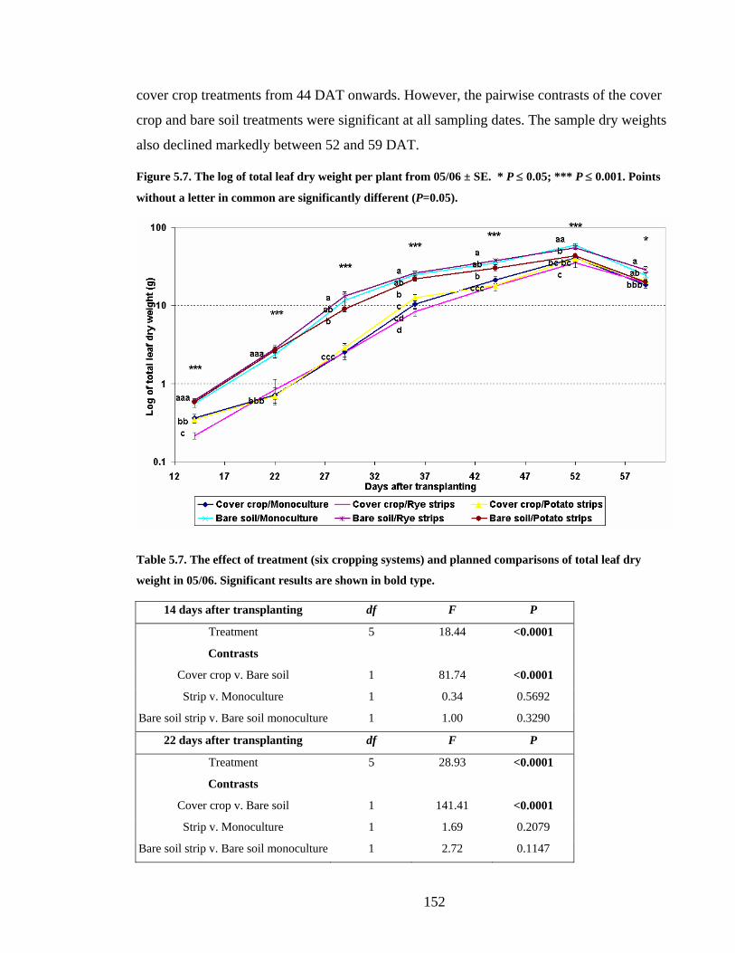
152
cover crop treatments from 44 DAT onwards. However, the pairwise contrasts of the cover
crop and bare soil treatments were significant at all sampling dates. The sample dry weights
also declined markedly between 52 and 59 DAT.
Figure 5.7. The log of total leaf dry weight per plant from 05/06 ± SE. * P ≤ 0.05; *** P ≤ 0.001. Points
without a letter in common are significantly different (P=0.05).
Table 5.7. The effect of treatment (six cropping systems) and planned comparisons of total leaf dry
weight in 05/06. Significant results are shown in bold type.
14 days after transplanting df F P
Treatment 5 18.44 <0.0001
Contrasts
Cover crop v. Bare soil 1 81.74 <0.0001
Strip v. Monoculture 1 0.34 0.5692
Bare soil strip v. Bare soil monoculture 1 1.00 0.3290
22 days after transplanting df F P
Treatment 5 28.93 <0.0001
Contrasts
Cover crop v. Bare soil 1 141.41 <0.0001
Strip v. Monoculture 1 1.69 0.2079
Bare soil strip v. Bare soil monoculture 1 2.72 0.1147

153
29 days after transplanting df F P
Treatment 5 19.45 <0.0001
Contrasts
Cover crop v. Bare soil 1 89.93 <0.0001
Strip v. Monoculture 1 0.03 0.8660
Bare soil strip v. Bare soil monoculture 1 0.12 0.7344
36 days after transplanting df F P
Treatment 5 39.40 <0.0001
Contrasts
Cover crop v. Bare soil 1 185.71 <0.0001
Strip v. Monoculture 1 0.20 0.6573
Bare soil strip v. Bare soil monoculture 1 0.50 0.4862
44 days after transplanting df F P
Treatment 5 18.36 <0.0001
Contrasts
Cover crop v. Bare soil 1 83.58 <0.0001
Strip v. Monoculture 1 1.68 0.2092
Bare soil strip v. Bare soil monoculture 1 0.25 0.6222
52 days after transplanting df F P
Treatment 5 12.37 <0.0001
Contrasts
Cover crop v. Bare soil 1 40.66 <0.0001
Strip v. Monoculture 1 8.17 0.0097
Bare soil strip v. Bare soil monoculture 1 9.83 0.0052
59 days after transplanting df F P
Treatment 5 3.33 0.0237
Contrasts
Cover crop v. Bare soil 1 7.52 0.0126
Strip v. Monoculture 1 0.12 0.7342
Bare soil strip v. Bare soil monoculture 1 0.01 0.9085
When the leaf dry weights were expressed on a per leaf basis there were significant
differences between the treatments at all sampling dates (Figure 5.8 and Table 5.8).
However, the differences between the treatments changed with time as the cover crop
treatment’s leaves were lighter than the bare soil treatments until 29 DAT, then at 44 DAT

154
and thereafter they became heavier than the bare soil treatments. These data combined with
that presented in Figure 5.6 and Figure 5.7, indicate that the cover crop treatments
accumulated less leaf biomass and had fewer but heavier leaves when compared to the bare
soil treatments. It should also be noted that the drop in leaf dry weight between 52 and 59
DAT was due to the senescence and detachment of the lower leaves.
Figure 5.8. Mean leaf dry weight in 05/06 ± SE. ** P ≤ 0.01; *** P ≤ 0.001. Points without a letter in
common are significantly different (P=0.05).
Table 5.8. The effect of treatment (six cropping systems) and planned comparisons of mean leaf dry
weight per plant in 05/06. Significant results are shown in bold type.
14 days after transplanting df F P
Treatment 5 28.28 <0.0001
Contrasts
Cover crop v. Bare soil 1 128.18 <0.0001
Strip v. Monoculture 1 1.54 0.2286
Bare soil strip v. Bare soil monoculture 1 0.32 0.5755

155
22 days after transplanting df F P
Treatment 5 12.42 <0.0001
Contrasts
Cover crop v. Bare soil 1 58.69 <0.0001
Strip v. Monoculture 1 1.76 0.2001
Bare soil strip v. Bare soil monoculture 1 1.90 0.1830
29 days after transplanting df F P
Treatment 5 12.32 <0.0001
Contrasts
Cover crop v. Bare soil 1 55.33 <0.0001
Strip v. Monoculture 1 0.00 0.9820
Bare soil strip v. Bare soil monoculture 1 0.10 0.7533
36 days after transplanting df F P
Treatment 5 4.74 0.0051
Contrasts
Cover crop v. Bare soil 1 0.12 0.7351
Strip v. Monoculture 1 0.00 0.9748
Bare soil strip v. Bare soil monoculture 1 3.64 0.0708
44 days after transplanting df F P
Treatment 5 10.12 <0.0001
Contrasts
Cover crop v. Bare soil 1 43.94 <0.0001
Strip v. Monoculture 1 2.02 0.1711
Bare soil strip v. Bare soil monoculture 1 0.11 0.7391
52 days after transplanting df F P
Treatment 5 61.65 <0.0001
Contrasts
Cover crop v. Bare soil 1 258.10 <0.0001
Strip v. Monoculture 1 11.73 0.0027
Bare soil strip v. Bare soil monoculture 1 1.71 0.2063
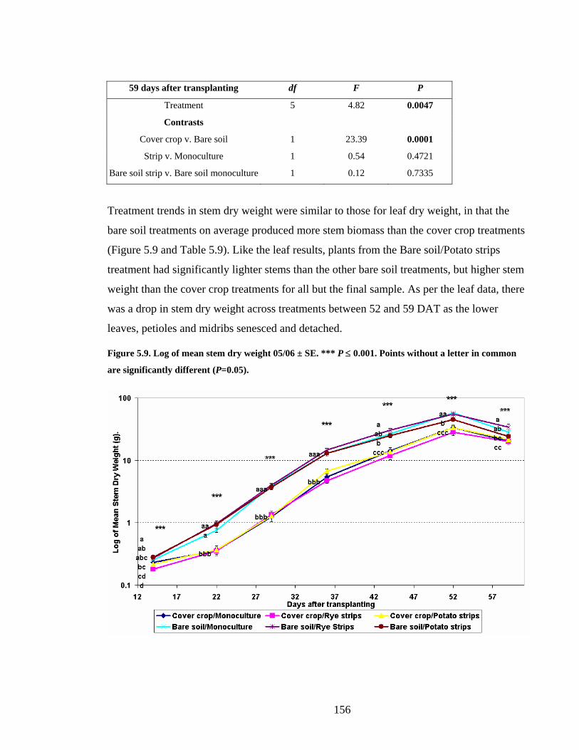
156
59 days after transplanting df F P
Treatment 5 4.82 0.0047
Contrasts
Cover crop v. Bare soil 1 23.39 0.0001
Strip v. Monoculture 1 0.54 0.4721
Bare soil strip v. Bare soil monoculture 1 0.12 0.7335
Treatment trends in stem dry weight were similar to those for leaf dry weight, in that the
bare soil treatments on average produced more stem biomass than the cover crop treatments
(Figure 5.9 and Table 5.9). Like the leaf results, plants from the Bare soil/Potato strips
treatment had significantly lighter stems than the other bare soil treatments, but higher stem
weight than the cover crop treatments for all but the final sample. As per the leaf data, there
was a drop in stem dry weight across treatments between 52 and 59 DAT as the lower
leaves, petioles and midribs senesced and detached.
Figure 5.9. Log of mean stem dry weight 05/06 ± SE. *** P ≤ 0.001. Points without a letter in common
are significantly different (P=0.05).

157
Table 5.9. The effect of treatment (six cropping systems) and planned comparisons of stem dry weight
in 05/06. Significant results are shown in bold type.
14 days after transplanting df F P
Treatment 5 8.04 0.0003
Contrasts
Cover crop v. Bare soil 1 30.46 <0.0001
Strip v. Monoculture 1 0.36 0.5569
Bare soil strip v. Bare soil monoculture 1 1.50 0.2350
22 days after transplanting df F P
Treatment 5 18.17 <0.0001
Contrasts
Cover crop v. Bare soil 1 85.85 <0.0001
Strip v. Monoculture 1 2.50 0.1296
Bare soil strip v. Bare soil monoculture 1 4.85 0.0395
29 days after transplanting df F P
Treatment 5 43.89 <0.0001
Contrasts
Cover crop v. Bare soil 1 218.37 <0.0001
Strip v. Monoculture 1 0.01 0.9236
Bare soil strip v. Bare soil monoculture 1 0.02 0.8921
36 days after transplanting df F P
Treatment 5 32.67 <0.0001
Contrasts
Cover crop v. Bare soil 1 157.14 <0.0001
Strip v. Monoculture 1 0.65 0.4298
Bare soil strip v. Bare soil monoculture 1 0.62 0.4394
44 days after transplanting df F P
Treatment 5 31.16 <0.0001
Contrasts
Cover crop v. Bare soil 1 146.93 <0.0001
Strip v. Monoculture 1 0.02 0.8760
Bare soil strip v. Bare soil monoculture 1 0.31 0.5824

158
52 days after transplanting df F P
Treatment 5 17.51 <0.0001
Contrasts
Cover crop v. Bare soil 1 75.76 <0.0001
Strip v. Monoculture 1 3.44 0.0784
Bare soil strip v. Bare soil monoculture 1 3.86 0.0636
59 days after transplanting df F P
Treatment 5 8.45 0.0002
Contrasts
Cover crop v. Bare soil 1 27.97 <0.0001
Strip v. Monoculture 1 0.15 0.7012
Bare soil strip v. Bare soil monoculture 1 0.14 0.7146
Analysis of the number of major branches arising from (and including) the main stem
indicates that the cover cropping treatments had significantly less additional branching than
the bare soil treatments (Figure 5.10 and Table 5.10). Amongst the bare soil treatments the
Bare soil/Potato strips treatment had significantly less additional branching at the later
sample than the Bare soil/Monoculture and the Bare soil/Rye strips treatments.
Figure 5.10. Mean number of branches arising from and including the main stem ± SE. *** P ≤ 0.001.
Treatments in each group without a letter in common are significantly different (P=0.05).

159
Table 5.10. The effect of treatment (six cropping systems) and planned comparisons of the number of
branches per plant in 05/06. Significant results are shown in bold type.
52 days after transplanting df F P
Treatment 5 86.18 <0.0001
Contrasts
Cover crop v. Bare soil 1 427.47 <0.0001
Strip v. Monoculture 1 0.00 1.0000
Bare soil strip v. Bare soil monoculture 1 0.20 0.6579
59 days after transplanting df F P
Treatment 5 52.71 <0.0001
Contrasts
Cover crop v. Bare soil 1 246.94 <0.0001
Strip v. Monoculture 1 0.92 0.3477
Bare soil strip v. Bare soil monoculture 1 6.60 0.0183
When the stem lengths of the broccoli plants were assessed there were significant
differences at each sampling date except at 44 DAT (Figure 5.11 and Table 5.11). The
cover crop treatments typically had longer stems early in the season as they grew out of the
cover crop. The sample taken 52 DAT indicated that plants from the Bare soil/Potato strips
treatment became the longest as competition for light with the neighbouring potato plants
strengthened. Up until the last sample the Bare soil/Monoculture treatment, which had the
least competition for light, had the shortest stems of all treatments.

160
Figure 5.11. Mean stem length of broccoli plants from 05/06 ± SE. “ns” not significant; * P ≤ 0.05; ** P
≤ 0.01; *** P ≤ 0.001. Points without a letter in common are significantly different (P=0.05).
Table 5.11. The effect of treatment (six cropping systems) and planned comparisons of stem length in
05/06. Significant results are shown in bold type.
22 days after transplanting df F P
Treatment 5 3.37 0.0228
Contrasts
Cover crop v. Bare soil 1 8.48 0.0086
Strip v. Monoculture 1 7.44 0.0130
Bare soil strip v. Bare soil monoculture 1 5.10 0.0352
29 days after transplanting df F P
Treatment 5 6.74 0.0008
Contrasts
Cover crop v. Bare soil 1 16.57 0.0006
Strip v. Monoculture 1 14.36 0.0011
Bare soil strip v. Bare soil monoculture 1 10.39 0.0043
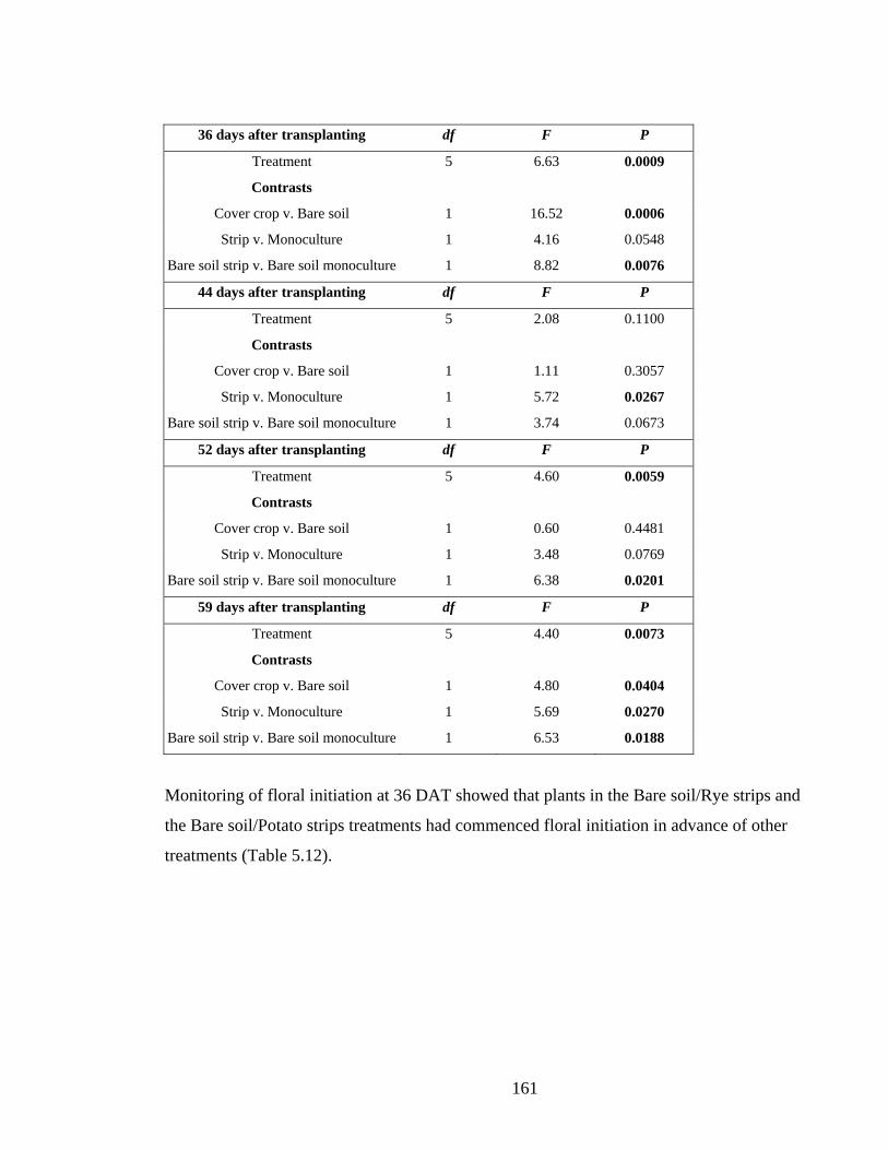
161
36 days after transplanting df F P
Treatment 5 6.63 0.0009
Contrasts
Cover crop v. Bare soil 1 16.52 0.0006
Strip v. Monoculture 1 4.16 0.0548
Bare soil strip v. Bare soil monoculture 1 8.82 0.0076
44 days after transplanting df F P
Treatment 5 2.08 0.1100
Contrasts
Cover crop v. Bare soil 1 1.11 0.3057
Strip v. Monoculture 1 5.72 0.0267
Bare soil strip v. Bare soil monoculture 1 3.74 0.0673
52 days after transplanting df F P
Treatment 5 4.60 0.0059
Contrasts
Cover crop v. Bare soil 1 0.60 0.4481
Strip v. Monoculture 1 3.48 0.0769
Bare soil strip v. Bare soil monoculture 1 6.38 0.0201
59 days after transplanting df F P
Treatment 5 4.40 0.0073
Contrasts
Cover crop v. Bare soil 1 4.80 0.0404
Strip v. Monoculture 1 5.69 0.0270
Bare soil strip v. Bare soil monoculture 1 6.53 0.0188
Monitoring of floral initiation at 36 DAT showed that plants in the Bare soil/Rye strips and
the Bare soil/Potato strips treatments had commenced floral initiation in advance of other
treatments (Table 5.12).
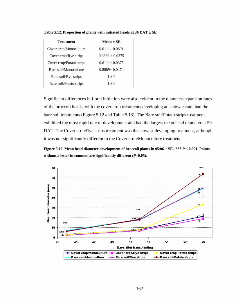
162
Table 5.12. Proportion of plants with initiated heads at 36 DAT ± SE.
Treatment Mean ± SE
Cover crop/Monoculture 0.6111± 0.0691
Cover crop/Rye strips 0.3889 ± 0.0375
Cover crop/Potato strips 0.6111± 0.0375
Bare soil/Monoculture 0.8889± 0.0474
Bare soil/Rye strips 1 ± 0
Bare soil/Potato strips 1 ± 0
Significant differences in floral initiation were also evident in the diameter expansion rates
of the broccoli heads, with the cover crop treatments developing at a slower rate than the
bare soil treatments (Figure 5.12 and Table 5.13). The Bare soil/Potato strips treatment
exhibited the most rapid rate of development and had the largest mean head diameter at 59
DAT. The Cover crop/Rye strips treatment was the slowest developing treatment, although
it was not significantly different to the Cover crop/Monoculture treatment.
Figure 5.12. Mean head diameter development of broccoli plants in 05/06 ± SE. *** P ≤ 0.001. Points
without a letter in common are significantly different (P=0.05).

163
Table 5.13. The effect of treatment (six cropping systems) and planned comparisons of head diameter
development in 05/06. Significant results are shown in bold type.
44 days after transplanting df F P
Treatment 5 28.94 <0.0001
Contrasts
Cover crop v. Bare soil 1 137.62 <0.0001
Strip v. Monoculture 1 4.30 0.0512
Bare soil strip v. Bare soil monoculture 1 2.98 0.0999
52 days after transplanting df F P
Treatment 5 30.58 <0.0001
Contrasts
Cover crop v. Bare soil 1 150.66 <0.0001
Strip v. Monoculture 1 0.14 0.7163
Bare soil strip v. Bare soil monoculture 1 0.01 0.9171
59 days after transplanting df F P
Treatment 5 18.78 <0.0001
Contrasts
Cover crop v. Bare soil 1 78.57 <0.0001
Strip v. Monoculture 1 2.99 0.0990
Bare soil strip v. Bare soil monoculture 1 2.22 0.1518
The number of days from transplant until harvest were similar in the 04/05 and the 05/06
experiment, with the cover crop treatments requiring approximately four to six days longer
to develop, while the Cover crop/Rye strips treatment developed slower than all the other
treatments (Figure 5.13 and Table 5.14). The faster development rate of the bare soil
treatments compared to the cover crop treatment was also demonstrated by the very
significant pairwise contrast.
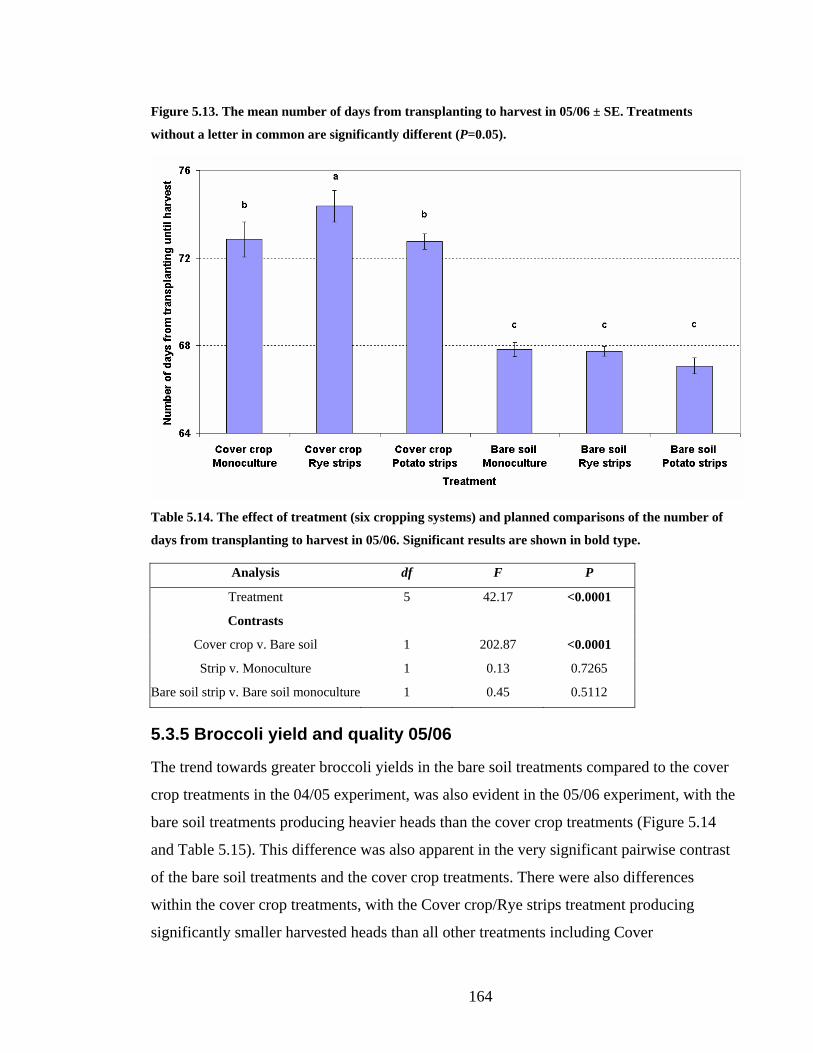
164
Figure 5.13. The mean number of days from transplanting to harvest in 05/06 ± SE. Treatments
without a letter in common are significantly different (P=0.05).
Table 5.14. The effect of treatment (six cropping systems) and planned comparisons of the number of
days from transplanting to harvest in 05/06. Significant results are shown in bold type.
Analysis df F P
Treatment 5 42.17 <0.0001
Contrasts
Cover crop v. Bare soil 1 202.87 <0.0001
Strip v. Monoculture 1 0.13 0.7265
Bare soil strip v. Bare soil monoculture 1 0.45 0.5112
5.3.5 Broccoli yield and quality 05/06
The trend towards greater broccoli yields in the bare soil treatments compared to the cover
crop treatments in the 04/05 experiment, was also evident in the 05/06 experiment, with the
bare soil treatments producing heavier heads than the cover crop treatments (Figure 5.14
and Table 5.15). This difference was also apparent in the very significant pairwise contrast
of the bare soil treatments and the cover crop treatments. There were also differences
within the cover crop treatments, with the Cover crop/Rye strips treatment producing
significantly smaller harvested heads than all other treatments including Cover
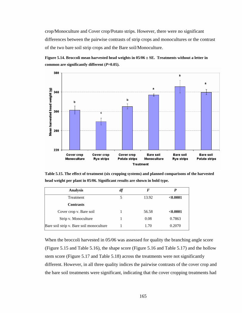
165
crop/Monoculture and Cover crop/Potato strips. However, there were no significant
differences between the pairwise contrasts of strip crops and monocultures or the contrast
of the two bare soil strip crops and the Bare soil/Monoculture.
Figure 5.14. Broccoli mean harvested head weights in 05/06 ± SE. Treatments without a letter in
common are significantly different (P=0.05).
Table 5.15. The effect of treatment (six cropping systems) and planned comparisons of the harvested
head weight per plant in 05/06. Significant results are shown in bold type.
Analysis df F P
Treatment 5 13.92 <0.0001
Contrasts
Cover crop v. Bare soil 1 56.58 <0.0001
Strip v. Monoculture 1 0.08 0.7863
Bare soil strip v. Bare soil monoculture 1 1.70 0.2070
When the broccoli harvested in 05/06 was assessed for quality the branching angle score
(Figure 5.15 and Table 5.16), the shape score (Figure 5.16 and Table 5.17) and the hollow
stem score (Figure 5.17 and Table 5.18) across the treatments were not significantly
different. However, in all three quality indices the pairwise contrasts of the cover crop and
the bare soil treatments were significant, indicating that the cover cropping treatments had

166
slightly better branching angle, shape and hollow stem scores and were therefore of
marginally better quality than the bare soil treatments.
Figure 5.15. Mean branching angle score (1-5) in 05/06 ± SE, where 1=worst branching angle
(unmarketable) and 5=best branching angle (highly marketable).
Table 5.16. The effect of treatment (six cropping systems) and planned comparisons of the branching
angle score in 05/06. Significant results are shown in bold type.
Analysis df F P
Treatment 5 1.13 0.3782
Contrasts
Cover crop v. Bare soil 1 5.23 0.0333
Strip v. Monoculture 1 0.04 0.8496
Bare soil strip v. Bare soil monoculture 1 0.00 0.9582

167
Figure 5.16. Mean shape score (1-5) in 05/06 ± SE, where 1=worst shape (unmarketable) and 5=best
shape (highly marketable).
Table 5.17. The effect of treatment (six cropping systems) and planned comparisons of the shape score
in 05/06. Significant results are shown in bold type.
Analysis df F P
Treatment 5 1.52 0.2282
Contrasts
Cover crop v. Bare soil 1 6.22 0.0215
Strip v. Monoculture 1 0.12 0.7335
Bare soil strip v. Bare soil monoculture 1 0.34 0.5680
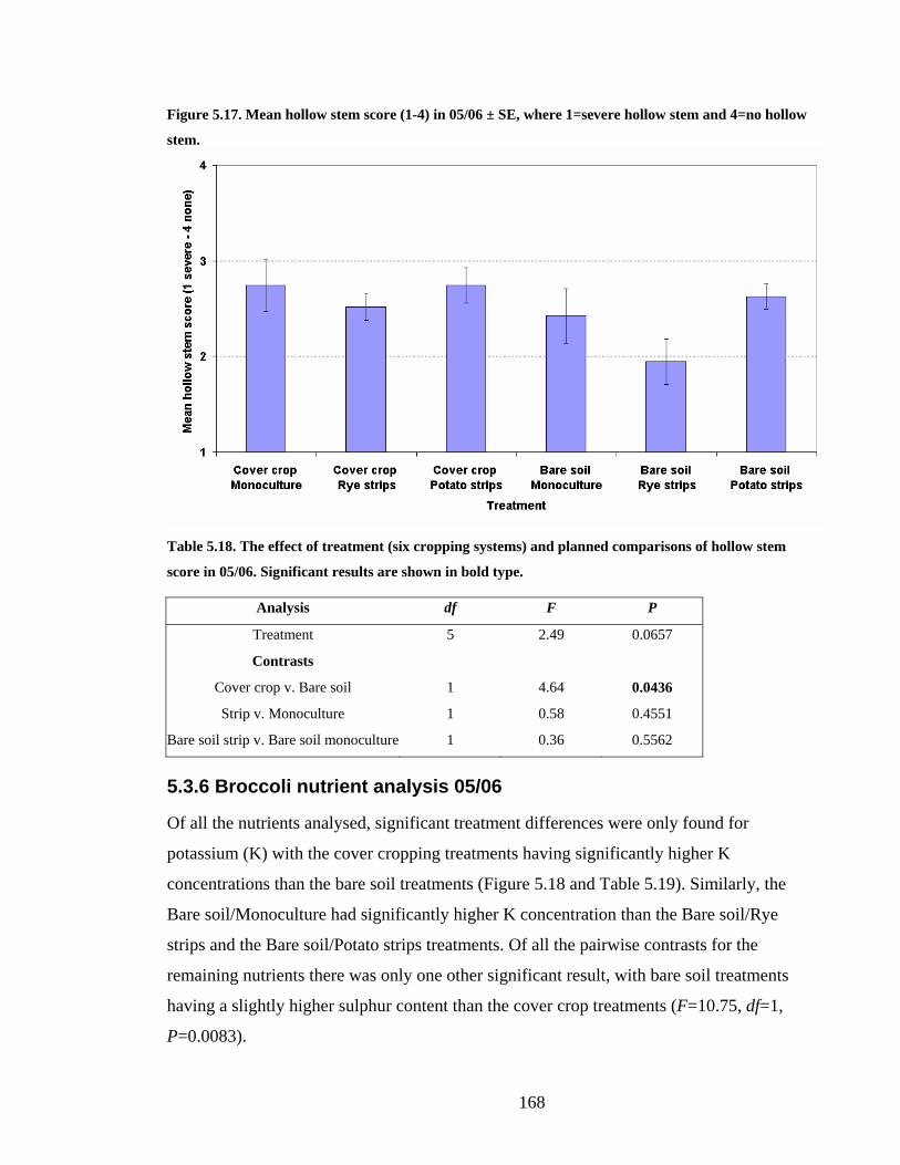
168
Figure 5.17. Mean hollow stem score (1-4) in 05/06 ± SE, where 1=severe hollow stem and 4=no hollow
stem.
Table 5.18. The effect of treatment (six cropping systems) and planned comparisons of hollow stem
score in 05/06. Significant results are shown in bold type.
Analysis df F P
Treatment 5 2.49 0.0657
Contrasts
Cover crop v. Bare soil 1 4.64 0.0436
Strip v. Monoculture 1 0.58 0.4551
Bare soil strip v. Bare soil monoculture 1 0.36 0.5562
5.3.6 Broccoli nutrient analysis 05/06
Of all the nutrients analysed, significant treatment differences were only found for
potassium (K) with the cover cropping treatments having significantly higher K
concentrations than the bare soil treatments (Figure 5.18 and Table 5.19). Similarly, the
Bare soil/Monoculture had significantly higher K concentration than the Bare soil/Rye
strips and the Bare soil/Potato strips treatments. Of all the pairwise contrasts for the
remaining nutrients there was only one other significant result, with bare soil treatments
having a slightly higher sulphur content than the cover crop treatments (F=10.75, df=1,
P=0.0083).
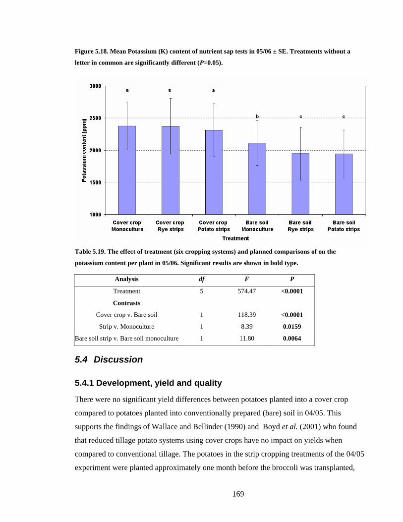
169
Figure 5.18. Mean Potassium (K) content of nutrient sap tests in 05/06 ± SE. Treatments without a
letter in common are significantly different (P=0.05).
Table 5.19. The effect of treatment (six cropping systems) and planned comparisons of on the
potassium content per plant in 05/06. Significant results are shown in bold type.
Analysis df F P
Treatment 5 574.47 <0.0001
Contrasts
Cover crop v. Bare soil 1 118.39 <0.0001
Strip v. Monoculture 1 8.39 0.0159
Bare soil strip v. Bare soil monoculture 1 11.80 0.0064
5.4 Discussion
5.4.1 Development, yield and quality
There were no significant yield differences between potatoes planted into a cover crop
compared to potatoes planted into conventionally prepared (bare) soil in 04/05. This
supports the findings of Wallace and Bellinder (1990) and Boyd et al. (2001) who found
that reduced tillage potato systems using cover crops have no impact on yields when
compared to conventional tillage. The potatoes in the strip cropping treatments of the 04/05
experiment were planted approximately one month before the broccoli was transplanted,
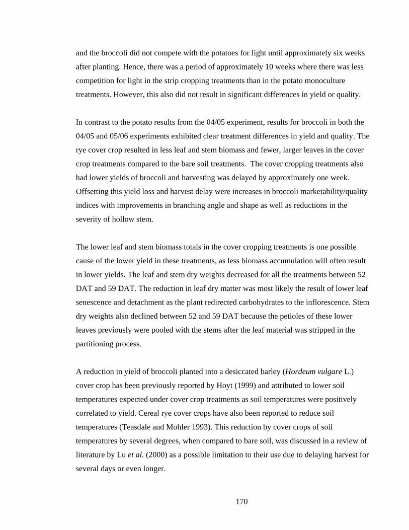
170
and the broccoli did not compete with the potatoes for light until approximately six weeks
after planting. Hence, there was a period of approximately 10 weeks where there was less
competition for light in the strip cropping treatments than in the potato monoculture
treatments. However, this also did not result in significant differences in yield or quality.
In contrast to the potato results from the 04/05 experiment, results for broccoli in both the
04/05 and 05/06 experiments exhibited clear treatment differences in yield and quality. The
rye cover crop resulted in less leaf and stem biomass and fewer, larger leaves in the cover
crop treatments compared to the bare soil treatments. The cover cropping treatments also
had lower yields of broccoli and harvesting was delayed by approximately one week.
Offsetting this yield loss and harvest delay were increases in broccoli marketability/quality
indices with improvements in branching angle and shape as well as reductions in the
severity of hollow stem.
The lower leaf and stem biomass totals in the cover cropping treatments is one possible
cause of the lower yield in these treatments, as less biomass accumulation will often result
in lower yields. The leaf and stem dry weights decreased for all the treatments between 52
DAT and 59 DAT. The reduction in leaf dry matter was most likely the result of lower leaf
senescence and detachment as the plant redirected carbohydrates to the inflorescence. Stem
dry weights also declined between 52 and 59 DAT because the petioles of these lower
leaves previously were pooled with the stems after the leaf material was stripped in the
partitioning process.
A reduction in yield of broccoli planted into a desiccated barley (Hordeum vulgare L.)
cover crop has been previously reported by Hoyt (1999) and attributed to lower soil
temperatures expected under cover crop treatments as soil temperatures were positively
correlated to yield. Cereal rye cover crops have also been reported to reduce soil
temperatures (Teasdale and Mohler 1993). This reduction by cover crops of soil
temperatures by several degrees, when compared to bare soil, was discussed in a review of
literature by Lu et al. (2000) as a possible limitation to their use due to delaying harvest for
several days or even longer.
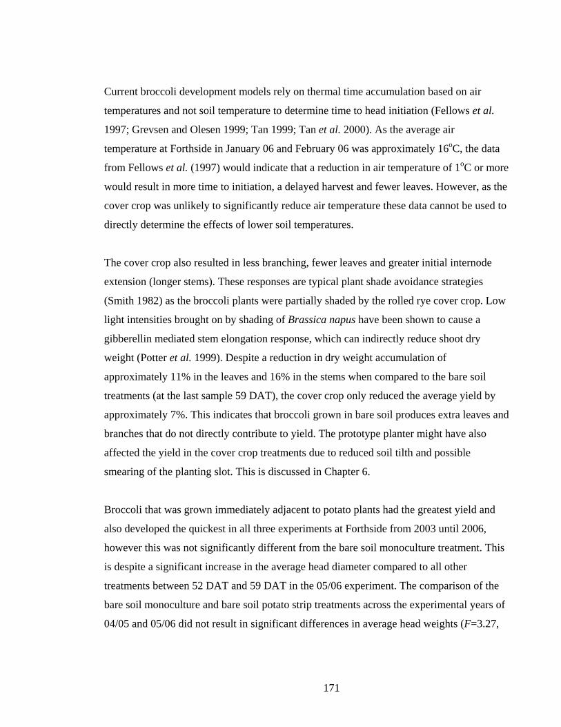
171
Current broccoli development models rely on thermal time accumulation based on air
temperatures and not soil temperature to determine time to head initiation (Fellows et al.
1997; Grevsen and Olesen 1999; Tan 1999; Tan et al. 2000). As the average air
temperature at Forthside in January 06 and February 06 was approximately 16oC, the data
from Fellows et al. (1997) would indicate that a reduction in air temperature of 1oC or more
would result in more time to initiation, a delayed harvest and fewer leaves. However, as the
cover crop was unlikely to significantly reduce air temperature these data cannot be used to
directly determine the effects of lower soil temperatures.
The cover crop also resulted in less branching, fewer leaves and greater initial internode
extension (longer stems). These responses are typical plant shade avoidance strategies
(Smith 1982) as the broccoli plants were partially shaded by the rolled rye cover crop. Low
light intensities brought on by shading of Brassica napus have been shown to cause a
gibberellin mediated stem elongation response, which can indirectly reduce shoot dry
weight (Potter et al. 1999). Despite a reduction in dry weight accumulation of
approximately 11% in the leaves and 16% in the stems when compared to the bare soil
treatments (at the last sample 59 DAT), the cover crop only reduced the average yield by
approximately 7%. This indicates that broccoli grown in bare soil produces extra leaves and
branches that do not directly contribute to yield. The prototype planter might have also
affected the yield in the cover crop treatments due to reduced soil tilth and possible
smearing of the planting slot. This is discussed in Chapter 6.
Broccoli that was grown immediately adjacent to potato plants had the greatest yield and
also developed the quickest in all three experiments at Forthside from 2003 until 2006,
however this was not significantly different from the bare soil monoculture treatment. This
is despite a significant increase in the average head diameter compared to all other
treatments between 52 DAT and 59 DAT in the 05/06 experiment. The comparison of the
bare soil monoculture and bare soil potato strip treatments across the experimental years of
04/05 and 05/06 did not result in significant differences in average head weights (F=3.27,
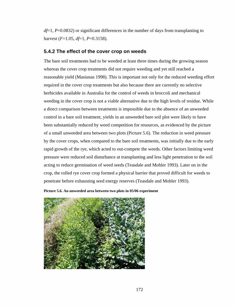
172
df=1, P=0.0832) or significant differences in the number of days from transplanting to
harvest (F=1.05, df=1, P=0.3158).
5.4.2 The effect of the cover crop on weeds
The bare soil treatments had to be weeded at least three times during the growing season
whereas the cover crop treatments did not require weeding and yet still reached a
reasonable yield (Masiunas 1998). This is important not only for the reduced weeding effort
required in the cover crop treatments but also because there are currently no selective
herbicides available in Australia for the control of weeds in broccoli and mechanical
weeding in the cover crop is not a viable alternative due to the high levels of residue. While
a direct comparison between treatments is impossible due to the absence of an unweeded
control in a bare soil treatment, yields in an unweeded bare soil plot were likely to have
been substantially reduced by weed competition for resources, as evidenced by the picture
of a small unweeded area between two plots (Picture 5.6). The reduction in weed pressure
by the cover crops, when compared to the bare soil treatments, was initially due to the early
rapid growth of the rye, which acted to out-compete the weeds. Other factors limiting weed
pressure were reduced soil disturbance at transplanting and less light penetration to the soil
acting to reduce germination of weed seeds (Teasdale and Mohler 1993). Later on in the
crop, the rolled rye cover crop formed a physical barrier that proved difficult for weeds to
penetrate before exhausting seed energy reserves (Teasdale and Mohler 1993).
Picture 5.6. An unweeded area between two plots in 05/06 experiment

173
Further evidence for the effectiveness of the cover crop in controlling weeds came from the
2004/2005 experiment. In this trial there was a strip of wild radish (Raphanus raphansitrum
L.) approximately 8m wide, which formed a thick carpet of seedlings that ran through the
length of the trial (all three repetitions). This was possibly due to past chemical trial
controls resulting in a huge seed bank in the soil. Wild radish is a very difficult weed to
control and is strongly competitive in all situations (Hyde-Wyatt and Morris 1975). Picture
5.7 and Picture 5.8 illustrate the differences between the cover crop and the bare soil
treatments. In Picture 5.7 the unweeded area between the different plots is covered in a
thick carpet of wild radish while the cover crop treatment on the right has the weed largely
under control.
Picture 5.7. Infestation of wild radish in the 04/05 experiment controlled by the rye cover crop on the
right, with the interplot region marked with a black line. Note that the plot pictured in Picture 5.8 is in
the background.
In Picture 5.8, even the cultivated areas between the two white markers have a significant
infestation of wild radish. This infestation required chemical treatment before planting and
significant manual weeding effort during the experiment, while the cover crop treatment
(Picture 5.9) had low levels of wild radish infestation and did not require weeding.
Therefore the cover crop had the ability to control this very invasive weed. However, to
achieve this level of weed control a dense, uniformly distributed cover crop must be
established prior to transplanting of the broccoli (Morse 1998).
174
Picture 5.8. Infestation of wild radish in a bare soil plot in the 04/05 experiment, with the interplot area
marked with a black line.
Picture 5.9. Control of wild radish by the unweeded cover crop at 48 DAP in the 04/05 experiment
5.4.3 Economic implications of the rye cover crop in broccoli cropping systems
Despite the positive effects of the cover crop treatments in reducing the levels of two
significant insect pests of broccoli (P. xylostella and B. brassicae) and hence a potential to
reduce control costs as well as a slight increase in quality of the harvested product, there
was a distinct negative impact on yield. It is important to determine if the negative impact
on yield is offset by the positive effects thus making the use of cover crops a economic
175
proposition for broccoli producers. Using the outcomes of this Chapter and Chapter 4 it is
possible to make an economic comparison of a broccoli production system using a rye
cover crop with that based on conventional cultivation. This comparison was conducted
using an enterprise budget and gross margin analysis based on an industry standard
produced by DPIW (2005) (Table 5.20). This standard has a number of assumptions and is
designed to be representative of what a competent operator, using industry standard
practices, might achieve on a model farm experiencing satisfactory seasonal conditions
(DPIW 2005). Some modification of these assumptions was needed to accommodate the
specifics of the two contrasting systems and these are marked with a superscript letter (a to
d). Yields estimates were derived from the treatment averages from the 05/06 experiment
so that harvest quality could also be taken into account by removing unmarketable broccoli
from the calculated means (that is, branching angle and shape scores of 1 and 2 as per
recommendations from Tan [1999]). Based on this approach, the average head weight for
the conventional practice (Bare soil/Monoculture) was 0.301 kg and the cover crop (Cover
crop/Monoculture) was 0.282 kg. These figures were then multiplied by the target density
of 33,000 plants/ha. In both the cover crop and the bare soil treatments the removal of the
previous crop would require some cultivation. Therefore this analysis assumes that the
cover crop was directly sown into the previous crop after this cultivation process using
minimum tillage, while the conventional system was left fallow (although it is becoming
increasingly common for farmers to plant a “green manure” crop of short-term grass to
increase organic matter in the cropping rotation and prevent erosion over the winter period).
Other assumptions were that the cover crop adequately suppressed weeds thus eliminating
the need for mechanical weeding and the cover crop reduced insect pressure so that only
one spray of insecticide for Lepidopteran larvae was required to ensure that the harvested
product met quality standards.
The enterprise budget and gross margin analysis indicates that even though the cover crop
system reduced the total variable costs by $323/ha (or 6.7%), the lower yield in the cover
crop treatment reduced the total gross margin by $151/ha (or 5.9%) when compared to
conventional practice of a bare soil monoculture. Based solely on these figures the practice
of using a cover crop would be less attractive than maintaining conventional practice.
176
However, the yield point at which the cover crop monoculture produced the same gross
margin as the bare soil monoculture was 9.507 tonnes/ha or 0.435 tonnes/ha less than the
bare soil monoculture. This would equate to a yield improvement in the cover crop
treatment of 0.202 tonnes/ha or just 2.2%, which with more research into transplanter
design (Chapter 6), tailoring fertiliser strategies for cover crops (not just using conventional
rates) and perhaps selecting cultivars more suitable to lower soil temperatures, is believed
to be achievable. Alternatively, a price premium of only 7% due to perceived (and actual)
improvements in the innate quality of the product through the use of a more ecologically
acceptable cropping method (Theunissen 1994), would have the same result as the 2.2%
yield increase.
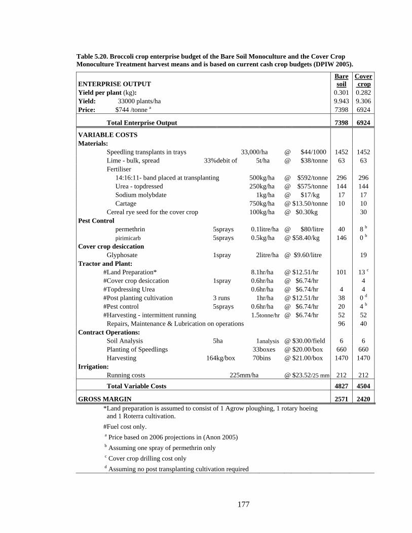
177
Table 5.20. Broccoli crop enterprise budget of the Bare Soil Monoculture and the Cover Crop Monoculture Treatment harvest means and is based on current cash crop budgets (DPIW 2005).
ENTERPRISE OUTPUT Bare soil
Cover crop
Yield per plant (kg): 0.301 0.282 Yield: 33000 plants/ha 9.943 9.306 Price: $744 /tonne a 7398 6924
Total Enterprise Output 7398 6924
VARIABLE COSTS Materials: Speedling transplants in trays 33,000/ha @ $44 /1000 1452 1452 Lime - bulk, spread 33%debit of 5t/ha @ $38 /tonne 63 63 Fertiliser 14:16:11- band placed at transplanting 500kg/ha @ $592 /tonne 296 296 Urea - topdressed 250kg/ha @ $575 /tonne 144 144 Sodium molybdate 1kg/ha @ $17 /kg 17 17 Cartage 750kg/ha @ $13.50 /tonne 10 10 Cereal rye seed for the cover crop 100kg/ha @ $0.30 kg 30 Pest Control permethrin 5sprays 0.1litre/ha @ $80 /litre 40 8 b pirimicarb 5sprays 0.5kg/ha @ $58.40 /kg 146 0 b Cover crop desiccation Glyphosate 1spray 2litre/ha @ $9.60/ litre 19 Tractor and Plant:
#Land Preparation* 8.1hr/ha @ $12.51 /hr 101 13 c #Cover crop desiccation 1spray 0.6hr/ha @ $6.74 /hr 4 #Topdressing Urea 0.6hr/ha @ $6.74 /hr 4 4 #Post planting cultivation 3 runs 1hr/ha @ $12.51 /hr 38 0 d #Pest control 5sprays 0.6hr/ha @ $6.74 /hr 20 4 b #Harvesting - intermittent running 1.5tonne/hr @ $6.74 /hr 52 52
Repairs, Maintenance & Lubrication on operations 96 40 Contract Operations: Soil Analysis 5ha 1analysis @ $30.00 /field 6 6 Planting of Speedlings 33boxes @ $20.00 /box 660 660 Harvesting 164kg/box 70bins @ $21.00 /box 1470 1470 Irrigation: Running costs 225mm/ha @ $23.52 /25 mm 212 212 Total Variable Costs 4827 4504
GROSS MARGIN 2571 2420 *Land preparation is assumed to consist of 1 Agrow ploughing, 1 rotary hoeing
and 1 Roterra cultivation. #Fuel cost only. a Price based on 2006 projections in (Anon 2005) b Assuming one spray of permethrin only c Cover crop drilling cost only d Assuming no post transplanting cultivation required

178
Chapter 6 Practical aspects of increasing crop species diversity: crop management and mechanisation A shift away from monocultures to strip or cover cropping would require some
modification to the way crops are managed. Changes would need to be made to land
preparation, planting, inter-row cultivation, spraying and harvesting activities. Some of
these aspects had to be addressed in this project, partly to ensure plots were managed
properly. This enabled examination of some of the practical issues farmers are likely to
confront if they decide to adopt these changes to their systems. Two novel pieces of
machinery were designed, built and trialled during the course of the project. These were a
five-metre wide low drift chemical spray unit and a broccoli roller/transplanter. This
chapter details the development and testing of these two pieces of equipment and the
associated rationale behind their development.
6.1 Development of a low drift spray unit
For the “Preliminary investigations” of 2003/2004 detailed in Chapter 3, each crop was
planted in 5m wide strips. Due to the size of the experimental area, chemical applications
with a small, knapsack type sprayer were impractical, which meant that the chemical
applications had to be from a tractor-based boom spray. Most spraying equipment used in
vegetable production systems in Tasmania are based on at least 12m boom widths and
would not fit a 5m wide system. It would have been possible to use one side of a 12m boom
spray on each strip, however this would have resulting in driving on the edge of each strip
and the zone of interaction between crops, which was of significant research interest. A
further problem was the potential for herbicides to “drift” into the neighbouring non-target
crops, again reducing production or possibly killing the neighbouring crops. Therefore it
was essential that a low drift, 5m spray rig be built in order to simplify management. This
design could potentially be applied to any strip width to facilitate management of a
commercialised strip cropping system.
Advice was obtained from a local spraying contractor Richard Murell from Beechworth
Spraying Pty Ltd (Ulverstone, Tasmania). Mr Murell recommended that the low drift spray

179
jets from Turbo Teejet® (Spraying Systems Co) be used (Picture 6.1.a). These particular
jets produce relatively large droplets when compared to fan jets, which when combined
with high water rates of 400L/ha and lower pressure, would significantly reduce spray drift.
A 400L spray unit (Hardi A/S, Taastrup, Denmark), seven Turbo Teejets® and spray tubing
were attached to a 6m boom so that the water fan created by the jets was projected slightly
forward and across the direction of motion (Picture 6.1.b). When the sprayer was calibrated
to use 400L/ha, there was adequate coverage and jet overlap for the 5m width. However,
the two outermost jets (one from each side) over sprayed the 5m by approximately 300mm.
Picture 6.1. (a). Side view of a Turbo Teejet® (left). (b). Assembling the sprayer (right).
This over-spray was controlled with an end guard constructed from a 7mm thick rubber
sheet with dimensions of 1m x 0.75m (Picture 6.2.a). The rubber was pop riveted onto a 1m
piece of 25mm angle iron, which was welded to a 150mm length of 60mm square tubing.
This tubing slid snugly over the spray boom and was fixed into position with two bolts
(Picture 6.2.b). As Picture 6.2.a illustrates, the square tubing was attached to the guard in an
offset position so that 400mm of the guard was in the direction of travel and 600mm was
effectively behind the jets. This was designed to minimise the spray drift that would follow
a tractor mounted sprayer. After initial trials, the edges of the rubber sheet were rounded to
prevent snagging on the soil and plant material. To keep the rubber guard stiff and therefore
straight, the end guard was also strengthened 100mm from the bottom edge by attaching a
25mm x 1m piece of flat bar (as indicated with a line of pop rivets from Picture 6.2.a).

180
Picture 6.2. (a). Sprayer end guard in profile with pop rivets indicated by the arrow (left). (b). The end
guard attachment (right).
These design changes meant that the sideways spray drift was contained. There was some
chemical runoff from the outer jet over-spray that hit the end guard, but this dripped out of
harms way between the plant rows and did not damage any crop plants.
Picture 6.3. The end guard between two crops.
Further testing indicated upward spray drift was not completely contained when the sprayer
was in operation. This was adequately contained by a sheet of nylon shade cloth stretched
over the top of the spray boom and left slightly hanging behind the sprayer (Picture 6.4.a
and Picture 6.4.b).

181
Picture 6.4. (a). Sprayer rear view (left). (b). The sprayer front view (right).
Once developed, the sprayer was used successfully used for all subsequent trial work in
03/04 and did not result in any adverse chemical damage to non-target neighbouring crops,
provided that the crop rows were correctly spaced.
6.2 Development of the roller/transplanter
Currently, there are no no-till transplanters or specialised cover crop rollers commercially
available in Australia. The lack of reliable no-till transplanters, resulting in inconsistent
stand establishment, has been discussed as a major limiting factor to the adoption of no-till
systems for transplanted crops (Morse 1998). Furthermore, to the best of the author’s
knowledge, there are no machines available that perform both tasks simultaneously. The
main rationale behind building the roller/transplanter was to demonstrate to farmers and
agronomists that broccoli could be mechanically transplanted into a cover crop and was
therefore a feasible alternative to current practices.
The development of the roller/transplanter began with the planting of the cover crop in the
2004/2005 trial. The first task was to desiccate and roll the cover crop to form a thick bed
of stem and leaf (Picture 6.5) (as discussed in Chapter 4).

182
Picture 6.5. Cover crop in the 04/05 experiment prior to desiccation and rolling.
The first attempt at rolling the cover crop was made with a conventional heavy roller with
two trailing discs aligned to form slots for the transplants to be set into (Picture 6.6.a) It
was immediately obvious that this roller was not suitable as the cover crop was not
flattened and sprang back into place. As time was limited due to the cover crop being
desiccated and the plantlets were on order, a manual solution had to be quickly developed.
As a temporary fix, the cover crop was manually flattened with a hand operated
crimping/flattening tool (Picture 6.6.b). This consisted of a 1.65m length of 40mm angle
iron with a sharpened edge attached to a handle, which was manually pressed with a foot
using body weight at approximately 200mm spacings, in much the same manner as spade is
used. This proved to be effective, which indicated that the rye cover crop could be crimped
and flattened with the downward pressure of body weight alone.
Picture 6.6. (a). The heavy roller with two trailing discs (left). (b). A demonstration of the angle iron
flattener (right).
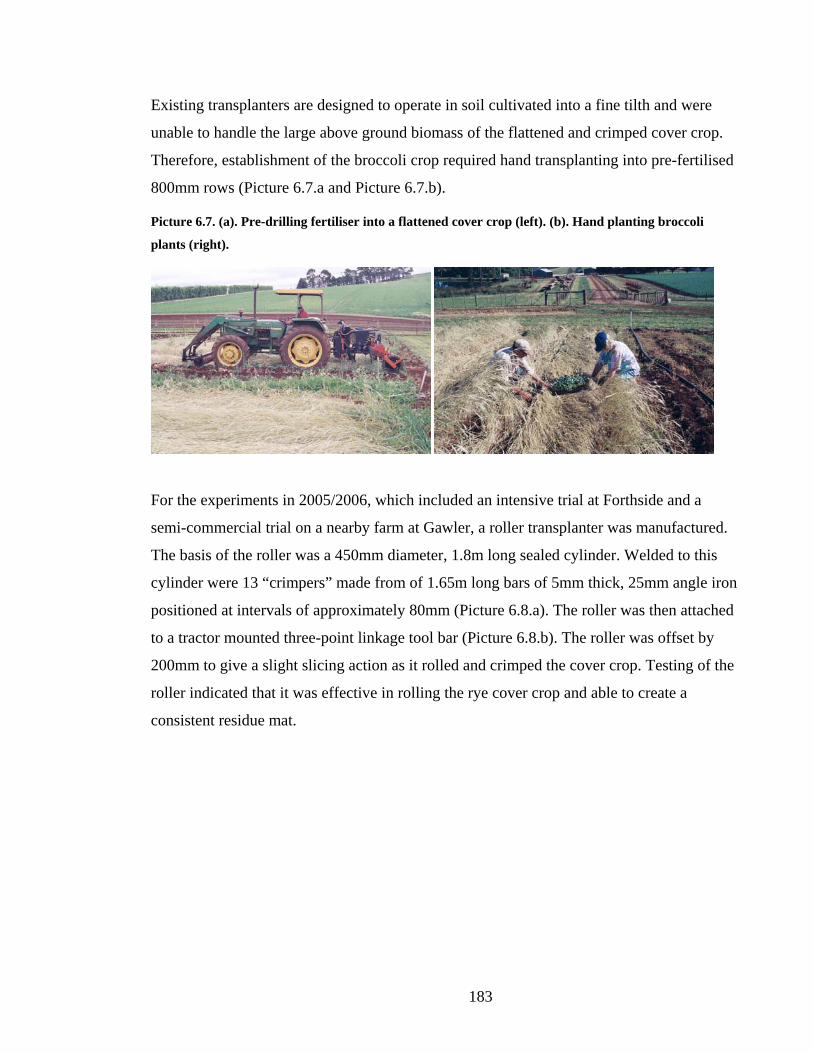
183
Existing transplanters are designed to operate in soil cultivated into a fine tilth and were
unable to handle the large above ground biomass of the flattened and crimped cover crop.
Therefore, establishment of the broccoli crop required hand transplanting into pre-fertilised
800mm rows (Picture 6.7.a and Picture 6.7.b).
Picture 6.7. (a). Pre-drilling fertiliser into a flattened cover crop (left). (b). Hand planting broccoli
plants (right).
For the experiments in 2005/2006, which included an intensive trial at Forthside and a
semi-commercial trial on a nearby farm at Gawler, a roller transplanter was manufactured.
The basis of the roller was a 450mm diameter, 1.8m long sealed cylinder. Welded to this
cylinder were 13 “crimpers” made from of 1.65m long bars of 5mm thick, 25mm angle iron
positioned at intervals of approximately 80mm (Picture 6.8.a). The roller was then attached
to a tractor mounted three-point linkage tool bar (Picture 6.8.b). The roller was offset by
200mm to give a slight slicing action as it rolled and crimped the cover crop. Testing of the
roller indicated that it was effective in rolling the rye cover crop and able to create a
consistent residue mat.

184
Picture 6.8. (a). Roller construction with the drum and angle iron “crimpers” indicated by the arrow
(left). (b). Attaching the roller to the tractor tool bar (right).
The next phase of the development process involved attaching a fertiliser box to the tool
bar. Having the roller offset meant that it was not practical for the fertiliser box to be driven
from the roller. Therefore a ground driven wheel was attached to drive the gears of the
fertiliser box (Picture 6.9.a). A horizontal piece of square tubing was also mounted on the
tool bar to attach two cup transplanter units (Picture 6.9.b).
Picture 6.9. (a). The roller with the fertiliser box attached indicated by the arrow (left). (b). A cup
planter unit indicated by the arrow (right).
The cup transplanters had no facility to drill fertiliser underneath the transplants. Therefore,
a set of double disc openers were made from two 450mm diameter straight edge discs and
attached to the cup planter (Picture 6.10.a). The double discs were touching at their leading
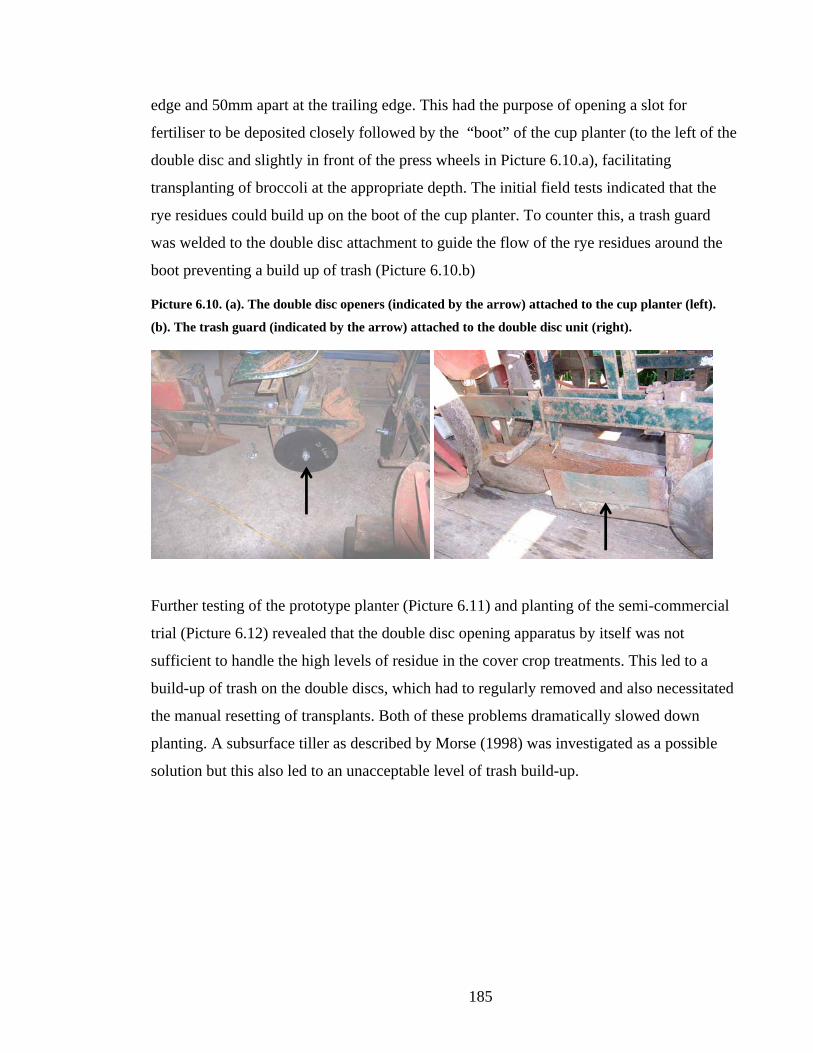
185
edge and 50mm apart at the trailing edge. This had the purpose of opening a slot for
fertiliser to be deposited closely followed by the “boot” of the cup planter (to the left of the
double disc and slightly in front of the press wheels in Picture 6.10.a), facilitating
transplanting of broccoli at the appropriate depth. The initial field tests indicated that the
rye residues could build up on the boot of the cup planter. To counter this, a trash guard
was welded to the double disc attachment to guide the flow of the rye residues around the
boot preventing a build up of trash (Picture 6.10.b)
Picture 6.10. (a). The double disc openers (indicated by the arrow) attached to the cup planter (left).
(b). The trash guard (indicated by the arrow) attached to the double disc unit (right).
Further testing of the prototype planter (Picture 6.11) and planting of the semi-commercial
trial (Picture 6.12) revealed that the double disc opening apparatus by itself was not
sufficient to handle the high levels of residue in the cover crop treatments. This led to a
build-up of trash on the double discs, which had to regularly removed and also necessitated
the manual resetting of transplants. Both of these problems dramatically slowed down
planting. A subsurface tiller as described by Morse (1998) was investigated as a possible
solution but this also led to an unacceptable level of trash build-up.
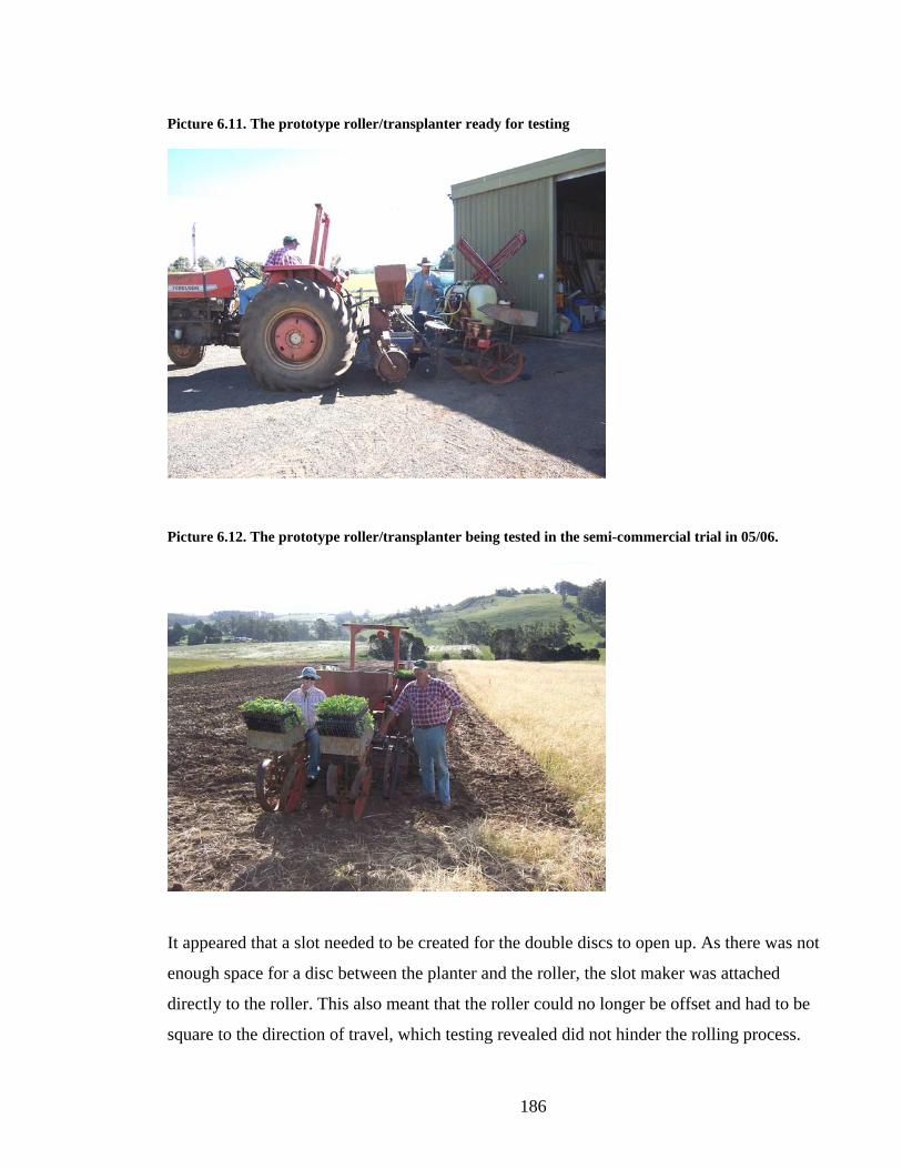
186
Picture 6.11. The prototype roller/transplanter ready for testing
Picture 6.12. The prototype roller/transplanter being tested in the semi-commercial trial in 05/06.
It appeared that a slot needed to be created for the double discs to open up. As there was not
enough space for a disc between the planter and the roller, the slot maker was attached
directly to the roller. This also meant that the roller could no longer be offset and had to be
square to the direction of travel, which testing revealed did not hinder the rolling process.
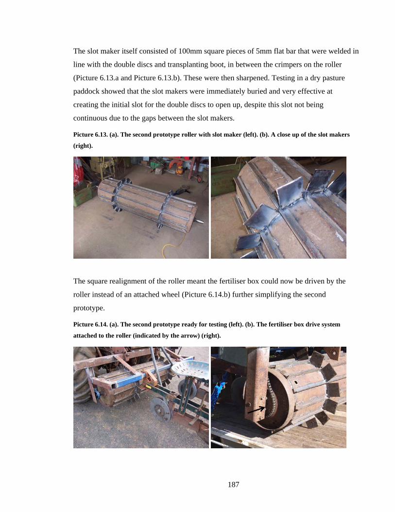
187
The slot maker itself consisted of 100mm square pieces of 5mm flat bar that were welded in
line with the double discs and transplanting boot, in between the crimpers on the roller
(Picture 6.13.a and Picture 6.13.b). These were then sharpened. Testing in a dry pasture
paddock showed that the slot makers were immediately buried and very effective at
creating the initial slot for the double discs to open up, despite this slot not being
continuous due to the gaps between the slot makers.
Picture 6.13. (a). The second prototype roller with slot maker (left). (b). A close up of the slot makers
(right).
The square realignment of the roller meant the fertiliser box could now be driven by the
roller instead of an attached wheel (Picture 6.14.b) further simplifying the second
prototype.
Picture 6.14. (a). The second prototype ready for testing (left). (b). The fertiliser box drive system
attached to the roller (indicated by the arrow) (right).

188
It was at this stage that the development process ended because the final trial had to be
planted. While the end result was acceptable (Picture 6.15) it was necessary to manually
check each transplant to ensure uniformity between bare soil (conventional) and cover crop
treatments.
Picture 6.15. The end result of the second prototype roller/transplanter, a rolled cover crop and
transplanted broccoli (Cover crop/Rye strips Treatment).
6.2.1 Potential improvement to the roller/transplanter
To improve planting efficiency a number of further design modifications need to be
considered including:
1. The addition of scrapers to remove soil that could build up on the slot makers
attached to the roller.
2. Heavier wheels for the cup planter set on a greater angle to the ground could assist
with pressing soil around the transplants and increasing soil contact.
3. The addition and modification of a subsurface tiller as described by Morse (1998) to
fracture the soil and improve stand establishment.
4. The addition of a fluted type disc coulter, which can improve soil flow back into the
slot formed, hence improving soil contact (Murray et al. 2006) with the transplant.

189
The last two points are important because the ferrosol (krasnozem) soil type on which the
research was conducted typically has a high clay content. Soil with a high clay content is
prone to smearing at the base and walls of the planting slot, which in extreme cases
prevents the plants roots from spreading outside the slot (Murray et al. 2006). Therefore,
any modification to the planter/roller that increased soil tilth in the slot created for the
transplants or soil flow back into the slot, has the potential to increase yields of the broccoli
when compared to the bare soil treatments.
6.3 Conclusion
This chapter demonstrates that it is possible to design, manufacture and successfully test
mechanical solutions to meet the needs of novel cropping systems. Therefore, the absence
of appropriate machinery should not be seen as a major barrier to the research and adoption
of alternative cropping practices (Vandermeer 1989).
190
Chapter 7 General Discussion The initial vision of this thesis was to investigate options for reducing the level of chemical
inputs in vegetable cropping systems, while maintaining efficiency and productivity. This
chapter discusses the major implications of this research and the relative sustainability of
the cover cropping system developed compared to current conventional practices. Then
future research directions and possible applications to other cropping systems are
highlighted.
7.1 Pest control implications of this research
The research conducted in this study has shown that it is possible to manage some insect
pests and weeds using a rye cover crop. Lewis et al. (1997) suggested that instead of
focusing on the development of new synthetic chemicals or promoting the use of more
benign or even “natural” chemicals like those extracted from Bacillus thuringensis,
research should work towards designing farming practices that work with nature in order to
prevent the elevation of an organism to pest status. The reduction in the prevalence of an
important insect pest like P. xylostella, and to a lesser extent B. brassicae, by the rye cover
crop, indicates that such a directional shift in agricultural research is plausible and that an
increase in plant species diversity can form part of an effective insect pest control strategy.
Conceptually, the cover crop acts like a broad-spectrum insecticide reducing, but not
necessarily eliminating pests (Finch and Collier 2003). However, unlike broad-spectrum
insecticides the overall reduction in numbers of P. xylostella eggs and larvae and B.
brassicae colonies also has the potential to increase the effectiveness of “soft” insecticides
(such as Bt formulations) and beneficial insects. These findings are of special significance
for the control of P. xylostella, as this insect has shown the ability to become resistant to
every insecticide applied in the field (Sarfraz et al. 2006). Furthermore, in Australia where
P. xylostella is typically the only major pest of Brassica crops (Baker and Kovaliski 1999),
there is no evidence of regional genetic differentiation of P. xylostella populations due to
frequent migration (Endersby et al. 2006), which means that insecticide resistance that
develops in one area has the potential to spread around the country. Therefore any non-
chemical control measures for P. xylostella could have important consequences for the
191
long-term production of vegetable Brassicas by potentially reducing insecticide use and/or
delaying the development of insecticide resistance.
7.2 Financial implications of this research
In addition to the potential to control insect pests and reduce insecticide use, this study has
shown that the rye cover crop can sufficiently suppress weeds to an extent that no
additional weed control strategies were required. However, this study has identified a
number of costs associated with cover crops. The rye cover crop changed the morphology,
growth and development of the broccoli plants to the extent that yield was reduced and
harvest time delayed by about a week. The negative impact of a yield reduction would be
offset to some degree by small gains observed in the quality indices of the broccoli crop
and cost reductions associated with reduced cultivation for weed control and fewer
insecticide applications. A financial analysis of the cost/benefit tradeoffs showed that
farmers would be marginally worse off adopting the revised cover crop based system, with
a 7% reduction in the gross margin obtained. However, a sensitivity analysis indicated that
minor improvements in yield (∼2%) or a small price premium (∼7%) would account for the
shortfall compared to the current system. The delay in harvest time is unlikely to be of
major concern as this is a fast growing crop that is ready for harvest in 9 to 10 weeks. One
extra week of growth is unlikely to hinder future cropping options and this can be factored
into planting schedules to ensure timeliness of supply to markets.
7.3 Environmental implications of this research
The costs and benefits of the rye cover crop are not purely financial as there are some
positive environmental outcomes that could be derived from using the revised system.
Conventional broccoli crops are typically planted into soil of a fine tilth, which requires
approximately three tractor operations using various implements. The subsequent crop
would then be weeded approximately three times using a tractor mounted inter-row cultivar
and sprayed up to five times with insecticides (DPIW 2005). The total number of
insecticide applications for the number of crops grown over a year could be as high as 35
(Baker and Kovaliski 1999). It is envisaged that the cover crop would be planted directly
into the previous crop after some minor cultivation with an implement like a rotary hoe.
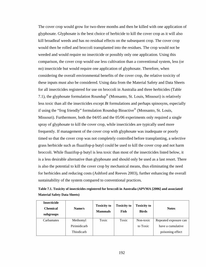
192
The cover crop would grow for two-three months and then be killed with one application of
glyphosate. Glyphosate is the best choice of herbicide to kill the cover crop as it will also
kill broadleaf weeds and has no residual effects on the subsequent crop. The cover crop
would then be rolled and broccoli transplanted into the residues. The crop would not be
weeded and would require no insecticide or possibly only one application. Using this
comparison, the cover crop would use less cultivation than a conventional system, less (or
no) insecticide but would require one application of glyphosate. Therefore, when
considering the overall environmental benefits of the cover crop, the relative toxicity of
these inputs must also be considered. Using data from the Material Safety and Data Sheets
for all insecticides registered for use on broccoli in Australia and three herbicides (Table
7.1), the glyphosate formulation Roundup® (Monsanto, St. Louis, Missouri) is relatively
less toxic than all the insecticides except Bt formulations and perhaps spinosyns, especially
if using the “frog friendly” formulation Roundup Bioactive® (Monsanto, St. Louis,
Missouri). Furthermore, both the 04/05 and the 05/06 experiments only required a single
spray of glyphosate to kill the cover crop, while insecticides are typically used more
frequently. If management of the cover crop with glyphosate was inadequate or poorly
timed so that the cover crop was not completely controlled before transplanting, a selective
grass herbicide such as fluazifop-p butyl could be used to kill the cover crop and not harm
broccoli. While fluazifop-p butyl is less toxic than most of the insecticides listed below, it
is a less desirable alternative than glyphosate and should only be used as a last resort. There
is also the potential to kill the cover crop by mechanical means, thus eliminating the need
for herbicides and reducing costs (Ashford and Reeves 2003), further enhancing the overall
sustainability of the system compared to conventional practices.
Table 7.1. Toxicity of insecticides registered for broccoli in Australia (APVMA [2006] and associated
Material Safety Data Sheets)
Insecticide
Chemical
subgroups
Name/s Toxicity to
Mammals
Toxicity to
Fish
Toxicity to
Birds Notes
Carbamates Methomyl
Pirimidicarb
Thiodicarb
Toxic Toxic Non-toxic
to Toxic
Repeated exposure can
have a cumulative
poisoning effect

193
Insecticide
Chemical
subgroups
Name/s Toxicity to
Mammals
Toxicity to
Fish
Toxicity to
Birds Notes
Organo-
phosphates
Chlorpyrifos
Diazinon
Dimethoate
Methamidophos
Phorate
Prothiofos
Trichlorfon
Toxic Toxic Toxic All are toxic and some
are very toxic. Can
cause kidney and liver
damage
Cylodiene Endosulfan Toxic Very toxic Toxic Kidneys, liver and
other organs can be
significantly affected
Phenylpyrazoles Fipronil Mildly toxic Toxic Can be
toxic
Can cause severe
irritation and damage
to the eye
Pyrethroids/
Pyrethrins
Alpha-
cypermethrin
Beta-cyfluthrin
Deltamethrin
Permethrin
Tau fluvalinate
Toxic Extremely
toxic
Toxic Can cause skin
sensitisation
Neonicotinoids Imidacloprid Non-toxic Toxic Toxic Rapidly immobilised
by the soil
Spinosyns Spinosad Non-toxic Slightly to
moderately
toxic
Non-toxic Relatively benign
product
Piridine
azomethine
Pymetrozine Non-toxic Non-toxic Non-toxic Antifeedant only active
on xylem feeders
Bacillus
thuringensis
Bacillus
thuringiensis
Non-toxic Non-toxic Non-toxic Toxic only to
caterpillars of certain
Lepidopterous insects
Chlorfenapyr Chlorfenapyr Toxic Toxic Toxic May adversely affect
mites predators and
other beneficials
Avermectin Emamectin
benzoate
Low toxicity Toxic Not stated Mild irritant
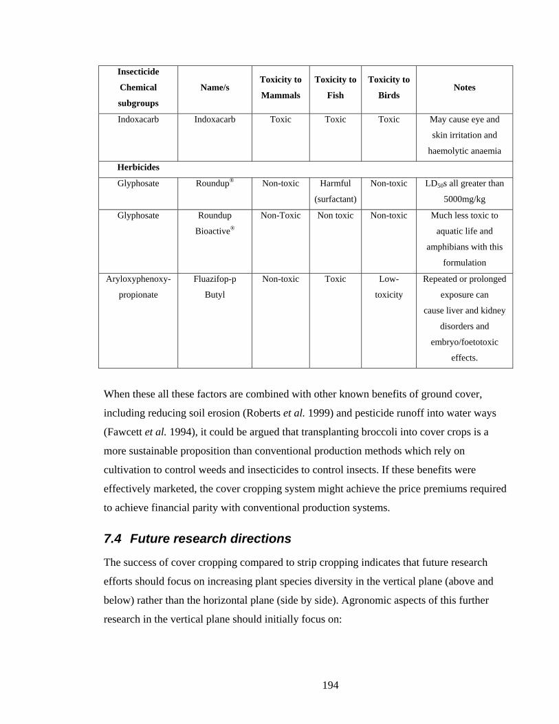
194
Insecticide
Chemical
subgroups
Name/s Toxicity to
Mammals
Toxicity to
Fish
Toxicity to
Birds Notes
Indoxacarb Indoxacarb Toxic Toxic Toxic May cause eye and
skin irritation and
haemolytic anaemia
Herbicides
Glyphosate Roundup® Non-toxic Harmful
(surfactant)
Non-toxic LD50s all greater than
5000mg/kg
Glyphosate Roundup
Bioactive®
Non-Toxic Non toxic Non-toxic Much less toxic to
aquatic life and
amphibians with this
formulation
Aryloxyphenoxy-
propionate
Fluazifop-p
Butyl
Non-toxic Toxic Low-
toxicity
Repeated or prolonged
exposure can
cause liver and kidney
disorders and
embryo/foetotoxic
effects.
When these all these factors are combined with other known benefits of ground cover,
including reducing soil erosion (Roberts et al. 1999) and pesticide runoff into water ways
(Fawcett et al. 1994), it could be argued that transplanting broccoli into cover crops is a
more sustainable proposition than conventional production methods which rely on
cultivation to control weeds and insecticides to control insects. If these benefits were
effectively marketed, the cover cropping system might achieve the price premiums required
to achieve financial parity with conventional production systems.
7.4 Future research directions
The success of cover cropping compared to strip cropping indicates that future research
efforts should focus on increasing plant species diversity in the vertical plane (above and
below) rather than the horizontal plane (side by side). Agronomic aspects of this further
research in the vertical plane should initially focus on:
195
• improving the design of the roller/transplanter to improve plant establishment and
yield through better transplant/soil contact and reduced soil smearing;
• identifying solutions to soil temperature constraints on growth, including the
selection of crop genotypes better suited to the system and altering planting dates;
• reducing the cost of production of the cover cropping system by including a
nitrogen fixing plant like a clover or vetch in the cover cropping to reduce the level
of nitrogenous fertiliser required; and
• determining minimum cover crop biomass requirements to improve planting
operations through residue reductions while also reducing seed costs and potential
crop competition.
The results from this study indicate that the effect of the cover crop on P. xylostella and B.
brassicae were due to interference with colonisation processes. However, it cannot be
determined if this interference caused female P. xylostella moths and alate B. brassicae to
emigrate from the area; have difficultly finding plants; or in the case of P. xylostella, lay
fewer eggs. Therefore further research should investigate the actual mechanism of this
colonisation interference. One possible research method could be the use of video
surveillance equipment to closely monitor P. xylostella and B. brassicae behaviour in a
similar fashion to experiments of Cleary et al. (2006) with Helicoverpa armigera
(Lepidoptera: Noctuidae).
The cover cropping strategy may be effective in other cropping systems with significant
insect pest issues, however generalisations regarding the impact of the rye cover crop on
the behaviour of insects are problematic due to the different behaviours of various pests, as
the results from P. rapae indicate. Therefore, the nature of the cover crop and its
management ought to be tailored to the specifics of the commercial crop in question and
should only be considered where it is able to significantly reduce populations of
economically significant insects. Reducing colonisation should be the aim of this
diversification strategy to keep infestations under the economic thresholds.

196
The study has also shown that a cover crop could be effective on small insects that are
relatively weak fliers with poorly directed flight, such as other species of aphids and
possibly thrips (Thysanoptera), as alate B. brassicae appeared to have difficulty
successfully locating host plants. There are already indications that rye residues negatively
affect thrips in cotton and peanuts (Olson et al. 2006). There are also indications that the
same mechanisms that inhibited P. xylostella host location might also operate on other
major Lepidopteran pests as wheat stubble can negatively impact Helicoverpa spp. in
cotton (Cleary et al. 2006). This could quite possibly be due to the adult Helicoverpa sp.,
like P. xylostella, being mainly active at night (Zalucki et al. 1986). Therefore adult insect
temporal (day/night) behaviour is worth further consideration as a possible component of
the mechanisms of the interference with colonisation processes in the cover crop.
197
Chapter 8 Summary of research findings The major findings from this research are:
• The rye cover crop significantly reduced the populations of P. xylostella and B.
brassicae presumably by interfering with host location/colonisation processes.
• The rye cover crop had no effect on P. rapae due to the insect’s highly developed
host location processes and random egg distribution behaviour.
• Strip cropping had no significant benefits and there were no additive effects as strip
cropping and cover cropping combined were no better than cover cropping alone.
• The cover crop significantly reduced plant biomass accumulation and yield, but
marginally improved quality.
• The economic analysis of the findings from this research revealed that the cover
crop reduced the gross margin of broccoli production by approximately 6% when
compared to conventional bare soil monocultures. However, this difference could be
eliminated by a 2.2% improvement in yield or a 7% price premium for using fewer
chemicals.
• It is possible to design, build and successfully test mechanical solutions to problems
associated with the cropping systems trialled, including accurate chemical
applications in strip crops and transplanting broccoli into a high biomass cover crop.
• Any interaction between plants in a strip cropping system are likely to occur in the
narrow zone where the plants are immediately adjacent to each other.
• Fungal diseases of the vegetable crops studied were too virulent and ubiquitous to
be controlled with strip cropping alone.
• Onions are poor competitors and not a suitable component of the strip cropping
system trialled.

198
References ABS (2003) Agricultural Commodities, ABS Catalogue 7121.0, Australian Bureau of
Statistics, Canberra.
Allen, P. and Kovach, M. (2000) The capitalist composition of organic: The potential of
markets in fulfilling the promise of organic agriculture. Agriculture and Human
Values 17: 221-232.
Altieri, M. A. (1998) Ecological impacts of industrial agriculture and the possibilities for
truly sustainable farming. Monthly Review-an Independent Socialist Magazine
50(3): 60-71.
Altieri, M. A. and Liebman, M. (1986) Insect, weed and plant disease management in
multiple cropping systems. In: C. A. Francis (Ed.) Multiple cropping systems,
MacMillan Publishing Co., N. Y., pp 183-218.
Altieri, M. A. and Rosset, P. M. (1996) Agroecology and the conversion of large-scale
conventional systems to sustainable management. International Journal of
Environmental Studies 50: 165-185.
Ames, B. N. and Gold, L. S. (1997) The causes and prevention of cancer: Gaining
perspective. Environmental Health Perspectives 105: 865-873.
Andow, D. A. (1991) Vegetational diversity and arthropod population response. Annual
Review of Entomology 36: 561-586.
Anon (2003a) Gene Technology Policy Review – Position Paper; A Balanced Approach.
Department of Primary Industries, Water and Environment. Hobart.
199
Anon (2003b) Tasmania's Natural Advantage,
http://www.dpiwe.tas.gov.au/inter.nsf/Attachments/TTAR-
5VW2Q4/$FILE/Tasmanias%20Natural%20Advantage.pdf, Accessed 23 May,
2003.
Anon (2003c) Tasmania's Vegetable and Associated Industries, Vegetable and Associated
Industries Branch, DPIWE, www.dpiwe.tas.gov.au, Accessed 23 May, 2003.
Anon (2005) Tasmanian Vegetable Industry Situation Paper 3, Tasmanian Government,
Hobart.
APVMA (2006) www.apvma.gov.au, Accessed 12 October, 2006.
Ashford, D. L. and Reeves, D. W. (2003) Use of a mechanical roller-crimper as an
alternative kill method for cover crops. American Journal of Alternative Agriculture
18(1): 37-45.
Åsman, K., Ekbom, B. and Rämert, B. (2001) Effect of intercropping on oviposition and
emigration behaviour of the leek moth (Lepidoptera: Acrolepiidae) and the
diamondback moth (Lepidoptera: Plutellidae). Environmental Entomology 30(2):
288-294.
ATTRA (1995) An Overview of Organic Production. In: Fundamentals of Sustainable
Agriculture. Online publication of: Appropriate Technology Transfer for Rural
Areas (ATTRA) Fayettville, USA, www.attra.org.
Ayisi, K. K., Putnam, D. H., Vance, C. P., Russelle, M. P. and Allan, D. L. (1997) Strip
intercropping and nitrogen effects on seed, oil, and protein yields of canola and
soybean. Agronomy Journal 89(1): 23-29.

200
Bach, C. E. and Tabashnik, B. E. (1990) Effects of nonhost plant neighbors on population
densities and parasitism rates of the diamondback moth (Lepidoptera: Plutellidae).
Environmental Entomology 19(4): 987-994.
Badenes-Perez, F. R., Shelton, A. M. and Nault, B. A. (2004) Evaluating trap crops for
diamondback moth, Plutella xylostella (Lepidoptera : Plutellidae). Journal of
Economic Entomology 97(4): 1365-1372.
Baker, G. (2004) Implementing Pest Management of Diamondback Moth, Project Number
VG00055, Horticulture Australia, Sydney NSW.
Baker, G. J. and Kovaliski, J. (1999) Detection of insecticide resistance in Plutella
xylostella (L.) (Lepidoptera: Plutellidae) populations in South Australian crucifer
crops. Australian Journal of Entomology 38(2): 132-134.
Banks, J. E. (1998) The scale of landscape fragmentation affects herbivore response to
vegetation heterogeneity. Oecologia 117(1-2): 239-246.
Banks, J. E. and Ekbom, B. (1999) Modelling herbivore movement and colonization: pest
management potential of intercropping and trap cropping. Agricultural and Forest
Entomology 1(3): 165-170.
Barr, N. (2004) The Micro-Dynamics of Change in Australian Agriculture 1976 – 2001.
Australian Bureau of Statistics. Canberra.
Baudry, J. and Papy, F. (2001) The role of landscape heterogeneity in the sustainability of
cropping systems. In: Crop science: progress and prospects. Papers presented at the
Third International Crop Science Congress, Hamburg, Germany, 17-22 August
2000. pp 243-259.
201
Bellinder, R. R., Wallace, R. W. and Wilkins, E. D. (1996) Reduced rates of herbicides
following hilling controlled weeds in conventional and reduced tillage potato
(Solanum tuberosum) production. Weed Technology 10(2): 311-316.
Boiffin, J., Malezieux, E. and Picard, D. (2001) Cropping systems for the future. In: Crop
science: progress and prospects. Papers presented at the Third International Crop
Science Congress, Hamburg, Germany, 17-22 August 2000. pp 261-279.
Bommarco, R. and Banks, J. E. (2003) Scale as modifier in vegetation diversity
experiments: effects on herbivores and predators. Oikos 102(2): 440-448.
Borowy, A. (2004) Effect of no-tillage and rye mulch on occurence of weeds and aphids
and on yields of cabbage, carrot and red beet. In: L. Bertschinger and J. D.
Anderson (Eds.), Proceedings of the XXVI International Horticultural Conference -
Sustainability of Horticultural Systems in the 21st Century, Toronto Canada, Acta
Horticulturae 638, pp 147-149
Bottenberg, H., Masiunas, J., Eastman, C. and Eastburn, D. (1997) Yield and quality
constraints of cabbage planted in rye mulch. Biological Agriculture & Horticulture
14: 323–342.
Boyd, N. S., Gordan, R., Asiedu, S. K. and Martin, R. C. (2001) The effects of living
mulches on tuber yield of potato (Solanum tuberosum L.). Biological Agriculture &
Horticulture 18: 203-220.
Brandsæter, L. O., Netland, J. and Meadow, R. (1998) Yields, weeds, pests and soil
nitrogen in a white cabbage living mulch system. Biological Agriculture &
Horticulture 16: 291-309.
Bravo, O. and Silenzi, J. C. (2002) Strip cropping in the semi-arid region of Argentina:
Control of wind erosion and soil water accumulation. Soil Science 167(5): 346-352.
202
Brewster, J. L. (1994) Onions and Other Edible Alliums. CAB International. Wallingford,
UK.
Brummer, E. C. (1998) Diversity, stability, and sustainable American agriculture.
Agronomy Journal 90(1): 1-2.
Bukovinszky, T., Potting, R. P. J., Clough, Y., van Lenteren, J. C. and Vet, L. E. M. (2005)
The role of pre- and post-alighting detection mechanisms in the responses to patch
size by specialist herbivores. Oikos 109(3): 435-446.
Bukovinszky, T., Trefas, H., van Lenteren, J. C., Vet, L. E. M. and Fremont, J. (2004) Plant
competition in pest-suppressive intercropping systems complicates evaluation of
herbivore responses. Agriculture Ecosystems & Environment 102(2): 185-196.
Clark, K. M. and Myers, R. L. (1994) Intercrop performance of pearl millet, amaranth,
cowpea, soybean, and guar in response to planting pattern and nitrogen fertilization.
Agronomy Journal 86(6): 1097-1102.
Cleary, A. J., Cribb, B. W. and Murray, D. A. H. (2006) Helicoverpa armigera (Hubner):
can wheat stubble protect cotton plants against attack? Australian Journal of
Entomology 45: 10-15.
Clunies-Ross, T. (1995) Mangolds, manure and mixtures. The importance of crop diversity
on British farms. Ecologist 25(5): 181-187.
Coeur, D. l., Baudry, J., Burel, F. and Thenail, C. (2002) Why and how we should study
field boundary biodiversity in an agrarian landscape context. Agriculture,
Ecosystems & Environment 89(1/2): 23-40.
203
Compton, S. G. (2002) Sailing with the wind: dispersal by small flying insects. In:
Dispersal ecology: The 42nd Symposium of the British Ecological Society held at
the University of Reading, UK on 2-5 April 2001. Oxford UK, Blackwell
Publishing, pp 113-133.
Conway, G. R. (1987) The Properties of Agroecosystems. Agricultural Systems 24(2): 95-
117.
Costello, M. J. (1994) Broccoli growth, yield and level of aphid infestation in leguminous
living mulches. Biological Agriculture & Horticulture 10: 207-222.
Costello, M. J. (1995) Spectral reflectance from a broccoli crop with vegetation or soil as
background: influence on immigration by Brevicoryne brassicae and Myzus
persicae. Entomologia Experimentalis et Applicata 75(2): 109–118.
Cotching, W. E., Hawkins, K., Sparrow, L. A., McCorkell, B. E. and Rowley, W. (2002)
Crop yields and soil properties on eroded slopes of red ferrosols in north-west
Tasmania. Australian Journal of Soil Research 40(4): 625-642.
Cromartie, W. J. (1975) The effect of stand size and vegetational background on the
colonisation of Cruciferous plants by herbivorous insects. Journal of Applied
Ecology 12: 517-533.
Dawson, T. and Fry, R. (1998) Agriculture in nature's image. Trends in Ecology and
Evolution 13(2): 50-51.
Denholm, I., Devine, G. J. and Williamson, M. S. (2002) Evolutionary genetics -
Insecticide resistance on the move. Science 297(5590): 2222-2223.
Dennis, J., Ed. (1997) Field Guide to Cream Gold Onion Disorders and Their Control in
Tasmania. Department of Primary Industries and Fisheries, Tasmania, Australia.

204
Donald, C., Endersby, N. M., Ridland, P. M., Porter, I. and Lawrence, J. (2000) Field Guide
to Pests, Diseases and Disorders of Vegetable Brassicas. Department of Natural
Resources, Victoria.
Doring, T. F., Kirchner, S. M., Kuhne, S. and Saucke, H. (2004) Response of alate aphids
to green targets on coloured backgrounds. Entomologia Experimentalis et Applicata
113(1): 53-61.
DPIW (2005) Crop enterprise budget - high rainfall,
http://www.dpiw.tas.gov.au/inter.nsf/Attachments/CART-
6FR6PZ/$FILE/HicropMaster2005.xls, Accessed 8 August, 2006.
Dueter, P. (1995) Broccoli. In: B. Coombs (Ed.) Horticulture Australia -The Complete
Reference of the Australian Horticultural Industry, Morescope Publishing:
Hawthorn East, Australia, pp 153-158.
Endersby, N. M., McKechnie, S. W., Ridland, P. M. and Weeks, A. R. (2006)
Microsatellites reveal a lack of structure in Australian populations of the
diamondback moth, Plutella xylostella (L.). Molecular Ecology 15(1): 107-118.
Fawcett, R. S., Christensen, B. R. and Tierney, D. P. (1994) The impact of conservation
tillage on pesticide runoff into surface water: a review and analysis. Journal of Soil
and Water Conservation 49(2): 126-135.
Fellows, J. R., Reader, R. J. and Wurr, D. C. E. (1997) A model for leaf production and
apex development in calabrese. Journal of Horticultural Science 72(2): 327-337.
Finch, S., Billiald, H. and Collier, R. H. (2003) Companion planting - do aromatic plants
disrupt host-plant finding by the cabbage root fly and the onion fly more effectively

205
than non-aromatic plants? Entomologia Experimentalis Et Applicata 109(3): 183-
195.
Finch, S. and Collier, R. H. (2000) Host-plant selection by insects - a theory based on
'appropriate/inappropriate landings' by pest insects of cruciferous plants.
Entomologia Experimentalis et Applicata 96(2): 91-102.
Finch, S. and Collier, R. H. (2003) Insects can see clearly now the weeds have gone.
Biologist 50(3): 132-135.
Finch, S. and Kienegger, M. (1997) A behavioural study to help clarify how undersowing
with clover affects host-plant selection by pest insects of brassica crops.
Entomologia Experimentalis Et Applicata 84(2): 165-172.
Finckh, M. R. and Mundt, C. C. (1992) Plant competition and disease in genetically diverse
wheat populations. Oecologia 91(1): 82-92.
Fitt, G. P. (1994) Cotton Pest-Management .3. An Australian Perspective. Annual Review of
Entomology 39: 543-562.
Furlong, M. J., Shi, Z., Liu, S. and Zalucki, M. P. (2004) Evaluation of the impact of
natural enemies on Plutella xylostella L. (Lepidoptera: Yponomeutidae) populations
on commercial Brassica farms. Agricultural and Forest Entomology 6(4): 311-322.
Garnaut, J. and Lim-Applegate, H. (1998) People in farming. ABARE. Canberra.
Garrett, K. A. and Mundt, C. C. (1999) Epidemiology in mixed host populations.
Phytopathology 89(11): 984-990.
Garrett, K. A., Nelson, R. J., Mundt, C. C., Chacon, G., Jaramillo, R. E. and Forbes, G. A.
(2001) The effects of host diversity and other management components on
206
epidemics of potato late blight in the humid highland tropics. Phytopathology
91(10): 993-1000.
Ghaffarzadeh, M., Prehac, F. G. and Cruse, R. M. (1997) Tillage effect on soil water
content and corn yield in a strip intercropping system. Agronomy Journal 89(6):
893-899.
Gill, S. S., Cowles, E. A. and Pietrantonio, P. V. (1992) The mode of action of Bacillus
thuringiensis endotoxins. Annual Review of Entomology(No. 37): 615-636.
Gilley, J. E., Kramer, L. A., Cruse, R. M. and Hull, A. (1997) Sediment movement within a
strip intercropping system. Journal of Soil and Water Conservation 52(6): 443-447.
Gilley, J. E., Risse, L. M. and Eghball, B. (2002) Managing runoff following manure
application. Journal of Soil and Water Conservation 57(6): 530-533.
Giulio, M. d., Edwards, P. J. and Meister, E. (2001) Enhancing insect diversity in
agricultural grasslands: the roles of management and landscape structure. Journal of
Applied Ecology 38(2): 310-319.
Grevsen, K. and Olesen, J. E. (1999) Modelling development of broccoli (Brassica
oleracea (L.) var. italica) from transplanting to head initiation. Journal of
Horticultural Science & Biotechnology 74(6): 698-705.
Gunningham, N. and Sinclair, D. (2002) Environmental Partnerships: Combining
Sustainability and Commercial Advantage in the Agricultural Sector, RIRDC
Publication No 02/004, pp 116.
Guthman, J. (2000) Raising organic: an agro-ecological assessment of grower practices in
California. Agriculture and Human Values 17(3): 257-266.
207
Hamilton, A. J., Schellhorn, N. A., Endersby, N. M., Ridland, P. M. and Ward, S. A. (2004)
A dynamic binomial sequential sampling plan for Plutella xylostella (Lepidoptera:
Plutellidae) on broccoli and cauliflower in Australia. Journal of Economic
Entomology 97(1): 127–135.
Harcourt, D. G. (1957) Biology of the diamondback moth, Plutella maculipennis (Curt.)
(Lepidoptera: Plutellidae), in Eastern Ontario. II. Life history, behaviour, and host
relationships. Canadian Entomologist 89: 554-564.
Hauggaard-Nielsen, H., Ambus, P. and Jensen, E. S. (2001) Interspecific competition, N
use and interference with weeds in pea-barley intercropping. Field Crops Research
70(2): 101-109.
Heap, I. M. (1997) The occurrence of herbicide-resistant weeds worldwide. Pesticide
Science 51(3): 235-243.
Hern, A., Edwards-Jones, G. and McKinlay, R. G. (1996) A review of the pre-oviposition
behaviour of the small cabbage white butterfly, Pieris rapae (Lepidoptera:
Pieridae). Annals of Applied Biology 128(2): 349-371.
Hill, L. (1993) Biological diversity in Tasmanian vegetable crops. In: R. Donaghey and K.
McKay (Eds.), Proceedings of the TCT-TFGA Nature Conservation Conference:
The Benefits of Sustaining Biological Diversity on the Farm, Tasmania, pp 71-93
Hokkanen, H. M. T. (1991) Trap cropping in pest management. Annual Review of
Entomology 36: 119-138.
Holt, J. S., Powles, S. B. and Holtum, J. A. M. (1993) Mechanisms and agronomic aspects
of herbicide resistance. Annual Review of Plant Physiology and Plant Molecular
Biology 44: 203-229.
208
Hooks, C. R. R. and Johnson, M. W. (2001) Broccoli growth parameters and level of head
infestations in simple and mixed plantings: impact of increased flora diversification.
Annals of Applied Biology 138(3): 269-280.
Hooks, C. R. R. and Johnson, M. W. (2003) Impact of agricultural diversification on the
insect community of cruciferous crops. Crop Protection 22(2): 223-238.
Horn, D. J. (1987) Vegetational background and parasitism of larval diamond-back moth
on collards. Entomologia Experimentalis et Applicata 43(3): 300-303.
Horn, P. A., de Boer, R. I. and Crawford, D. J. (2002) A Field Guide to Insects and
Diseases of Australian Potato Crops. Melbourne University Press, Melbourne.
Hoyt, G. D. (1999) Tillage and cover residue effects on vegetable yields. HortTechnology
9(3): 351-358.
Hughes, R. D. (1963) Population dynamics of the cabbage aphid, Brevicoryne brassicae
(L.). Journal of Animal Ecology 32(3): 393-424.
Hyde-Wyatt, B. S. and Morris, D. I. (1975) Tasmanian Weed Handbook. Department of
Agriculture, Tasmania.
Infante, M. L. and Morse, R. D. (1996) Integration of no tillage and overseeded legume
living mulches for transplanted broccoli production. HortScience 31: 376-379.
Jackson, W. (2002) Natural systems agriculture: a truly radical alternative. Agriculture,
Ecosystems & Environment 88(2): 111-117.
Jolliffe, P. A. (1997) Are mixed populations of plant species more productive than pure
stands? Oikos 80(3): 595-602.
209
Keating, B. A. and Carberry, P. S. (1993) Resource capture and use in intercropping: solar
radiation. Field Crops Research 34(3-4): 273-301.
Keller, M. A. and Baker, G. (2003) Impact of conservation biological control practices on
natural enemies: a case study of diamondback moth and its parasitoids. In:
Proceedings of the 1st International Symposium on Biological Control of
Arthropods, Honolulu, Hawaii, 14-18 January 2002. Washington USA, United
States Department of Agriculture Forest Service, pp 215-219.
Kennedy, J. S., Booth, C. O. and Kershaw, W. J. S. (1961) Host finding by aphids in the
field: III. Visual attraction. Annals of Applied Biology 49: 1-21.
Kfir, R. (1998) Origin of the diamondback moth (Lepidoptera : Plutellidae). Annals of the
Entomological Society of America 91(2): 164-167.
Kirkman, R. (1995) Potatoes. In: B. Coombs (Ed) Horticulture Australia -The Complete
Reference of the Australian Horticultural Industry. Morescope Publishing:
Hawthorn East, Australia, pp 250-256.
Knickel, K. (1990) Agricultural structural-change - impact on the rural environment.
Journal of Rural Studies 6(4): 383-393.
Kondinin-Group (2000) Organic Farming in Australia. RIRDC, Barton ACT.
Kostal, V. and Finch, S. (1994) Influence of background on host-plant selection and
subsequent oviposition by the cabbage root fly (Delia radicum). Entomologia
Experimentalis Et Applicata 70(2): 153-163.
Kuepper, G. and Dodson, M. (2001) Companion Planting: Basic Concepts & Resources.
Online publication of: Appropriate Technology Transfer for Rural Areas (ATTRA)
Fayettville, USA,<www.attra.org>.

210
Laurence, R. (2000) Sustainable and Intensive Cropping Systems: a feasibility study.
RIRDC, Barton, ACT.
Legg, W. and Viatte, G. (2001) Farming systems for sustainable agriculture. OECD
Observer 226-227: 21-24.
Lesoing, G. W. and Francis, C. A. (1999) Strip intercropping effects on yield and yield
components of corn, grain sorghum, and soybean. Agronomy Journal 91(5): 807-
813.
Lewis, W. J., vanLenteren, J. C., Phatak, S. C. and Tumlinson, J. H. (1997) A total system
approach to sustainable pest management. Proceedings of the National Academy of
Sciences of the United States of America 94(23): 12243-12248.
Liebman, M. and Dyck, E. (1993) Crop rotation and intercropping strategies for weed
management. Ecological Applications 3(1): 92-122.
Lotter, D. W. (2003) Organic agriculture. Journal of Sustainable Agriculture 21(4): 59-128.
Lotz, L. A. P., Groeneveld, R. M. W., Theunissen, J. and Broek, R. C. F. M. v. d. (1997)
Yield losses of white cabbage caused by competition with clovers grown as cover
crop. Netherlands Journal of Agricultural Science. 45: 393-405.
Lu, Y., Watkins, K. B., Teasdale, J. R. and Abdul-Baki, A. A. (2000) Cover crops in
sustainable food production. Food Reviews International 16(2): 121-157.
Luther, G. C., Valenzuela, H. R. and Defrank, J. (1996) Impact of cruciferous trap crops on
lepidopteran pests of cabbage in Hawaii. Environmental Entomology 25(1): 39-47.

211
Mangan, F., DeGregorio, R., Schonbeck, M., Herbert, S., Guillard, K., Hazzard, R.,
Sideman, E. and Litchfield, G. (1995) Cover cropping systems for brassicas in the
northeastern United States: 2. Weed, insect and slug incidence. Journal of
Sustainable Agriculture 5(3): 15-36.
Marazzi, C., Patrian, B. and Stadler, E. (2004) Secondary metabolites of the leaf surface
affected by sulphur fertilization and perceived by the diamondback moth.
Chemoecology 14(2): 81-86.
Marazzi, C. and Stadler, E. (2004) Influence of plant sulphur nutrition on oviposition and
larval performance of the diamondback moth. Entomologia Experimentalis et
Applicata 111(3): 225-232.
Marshall, E. J. P. (2002) Introducing field margin ecology in Europe. Agriculture,
Ecosystems & Environment 89(1/2): 1-4.
Marshall, E. J. P., Brown, V. K., Boatman, N. D., Lutman, P. J. W., Squire, G. R. and
Ward, L. K. (2003) The role of weeds in supporting biological diversity within crop
fields. Weed Research 43(2): 77-89.
Marshall, E. J. P. and Moonen, A. C. (2002) Field margins in northern Europe: their
functions and interactions with agriculture. Agriculture, Ecosystems & Environment
89(1/2): 5-21.
Martinez-Ghersa, M. A., Worster, C. A. and Radosevich, S. R. (2003) Concerns a weed
scientist might have about herbicide-tolerant crops: A revisitation. Weed
Technology 17(1): 202-210.
Masiunas, J. B. (1998) Production of vegetables using cover crop and living mulches - a
review. Journal of Vegetable and Crop Production 4(1): 11-31.
212
Masiunas, J. B., Eastburn, D. M., Mwaja, V. N. and Eastman, C. E. (1997) The impact of
living and cover crop mulch systems on pests and yields of snap beans and cabbage.
Journal of Sustainable Agriculture 9(2/3): 131-155.
Matson, P. A., Parton, W. J., Power, A. G. and Swift, M. J. (1997) Agricultural
intensification and ecosystem properties. Science 277(5325): 504-509.
McCann, K. S. (2000) The diversity-stability debate. Nature 405(6783): 228-233.
Meena, R. K. and Lal, O. P. (2002) Effect of intercropping on the incidence of
diamondback moth, Plutella xylostella (L.) on cabbage. Journal of Entomological
Research 26(2): 141-144.
Mensah, R. K. (1999) Habitat diversity: implications for the conservation and use of
predatory insects of Helicoverpa spp. in cotton systems in Australia. International
Journal of Pest Management 45(2): 91-100.
Miller, L. (1995) Agribusiness, Contract Farmers and Land-Use Sustainability in North-
West Tasmania. Australian Geographer 26(2): 104-111.
Mo, J., Baker, G., Keller, M. and Roush, R. (2003) Local dispersal of the diamondback
moth (Plutella xylostella (L.)) (Lepidoptera: Plutellidae). Environmental
Entomology 32(1): 71-79.
Mo, J. H. and Baker, G. (2004) Evaluation of sequential presence-absence sampling plans
for the diamondback moth (Plutellidae: Lepidoptera) in cruciferous crops in
Australia. Journal of Economic Entomology 97(3): 1118-1125.
Moriuti, S. (1986) Taxonomic notes on the diamondback moth. In: Diamondback Moth
Management. Proceedings of the First International Workshop, Tainan, Taiwan, 11-
15 March, 1985. pp 83-88.
213
Morse, R. D. (1998) Keys to successful production of transplanted crops in high residue,
no-till planting systems. In: T. C. Keisling (Ed.), Proceedings of the 21st Annual
Southern Conservation Tillage Conference for Sustainable Agriculture, North Little
Rock, Arkansas, 15-17 July, pp 79-82
Muggeridge , J. (1942) The white butterfly (Pieris rapae L.) I. Its establishment, spread,
and control in New Zealand. The New Zealand Journal of Science and Technology
24(3A): 107-129.
Mundt, C. C. (2002) Use of multiline cultivars and cultivar mixtures for disease
management. Annual Review of Phytopathology 40: 381-410.
Mundt, C. C., Cowger, C. and Garrett, K. A. (2002) Relevance of integrated disease
management to resistance durability. Euphytica 124(2): 245-252.
Murray, J. R., Tullberg, J. N. and Basnet, B. B. (2006) Planters and their components -
types, attributes, functional requirements and description. The Australian Centre for
International Agricultural Research, Monograph No. 121, Canberra.
Mwaja, V. N., Masiunas, J. B. and Eastman, C. E. (1996) Rye (Secale cereale L.) and hairy
vetch (Vicia villosa Roth) intercrop management in fresh-market vegetables.
Journal of the American Society for Horticultural Science 121(3): 586-591.
Nelson, W. A., Kahn, B. A. and Roberts, B. W. (1991) Screening cover crops for use in
conservation tillage systems for vegetables following spring plowing. HortScience
26: 860-862.
Nottingham, S. F., Hardie, J., Dawson, G. W., Hick, A. J., Pickett, J. A., Wadhams, L. J.
and Woodcock, C. M. (1991) Behavioural and electrophysiological responses of

214
aphids to host and nonhost plant volatiles. Journal of Chemical Ecology 17(6):
1231-1242.
Ntahimpera, N., Ellis, M. A., Wilson, L. L. and Madden, L. V. (1998) Effects of a cover
crop on splash dispersal of Colletotrichum acutatum conidia. Phytopathology 88(6):
536-543.
O'Donnell, D., Vujovic, S., Poynter, B. and Morgan, W. (1998) Quality Description
Language - Broccoli. ExpHort 2000 Publication No. 53, Department of Natural
Resources and Environment, Knoxville, Victoria.
Olson, D. M., Davis, R. F., Brown, S. L., Roberts, P. and Phatak, S. C. (2006) Cover crop,
rye residue and in-furrow treatment effects on thrips. Journal of Applied
Entomology 130(5): 302–308.
Parkhurst, A. M. and Francis, C. A. (1986) Research methods for multiple cropping. In: C.
A. Francis (Ed.) Multiple Cropping Systems. New York, Macmillian Publishing
Company, pp 285-316.
Peach, L., Benjamin, L. A. and Mead, A. (2000) Effects on the growth of carrots (Daucus
carota L.), cabbage (Brassica oleracea var. capitata L.) and onion (Allium cepa L.)
of restricting the ability of the plants to intercept resources. Journal of Experimental
Botany 51(344): 605-615.
Petersen, R. G. (1994) Agricultural Field Experiments: Design and Analysis. Marcel
Dekker Inc, New York.
Pimentel, D., Stachow, U., Takacs, D. A., Brubaker, H. W., Dumas, A. R., Meaney, J. J.,
O'Neil, J. A. S., Onsi, D. E. and Corzilius, D. B. (1992) Conserving biological
diversity in agricultural/forestry systems. BioScience 42(5): 354-362.

215
Potter, T. I., Rood, S. B. and Zanewich, K. P. (1999) Light intensity, gibberellin content
and the resolution of shoot growth in Brassica. Planta 207(4): 505-511.
Potting, R. P. J., Perry, J. N. and Powell, W. (2005) Insect behavioural ecology and other
factors affecting the control efficacy of agro-ecosystern diversification strategies.
Ecological Modelling 182(2): 199-216.
Potts, M. J. (1990) Influence of intercropping in warm climates on pests and diseases of
potato, with special reference to their control. Field Crops Research 25(1-2): 133-
144.
Poudel, D. D., Midmore, D. J. and West, L. T. (1999) Erosion and productivity of vegetable
systems on sloping volcanic ash-derived Philippine soils. Soil Science Society of
America Journal 63(5): 1366-1376.
Prokopy, R. J. and Owens, E. D. (1983) Visual detection of plants by herbivorous insects.
Annual Review of Entomology 28: 337-364.
Rämert, B. (2002) The use of mixed species cropping to manage pests and diseases - theory
and practice. In: Powell et. al (Eds.) UK Organic Research 2002: Proceedings of the
COR Conference, Aberystwyth, pp 207-210
Reed, D. W., Pivnick, K. A. and Underhill, E. W. (1989) Identification of chemical
oviposition stimulants for the diamondback moth, Plutella xylostella, present in
three species of Brassicaceae. Entomologia Experimentalis et Applicata 53(3): 277-
286.
Renwick, J. A. A. and Chew, F. S. (1994) Oviposition behaviour in Lepidoptera. Annual
Review of Entomology 39: 377-400.
216
Richards, O. W. (1940) The biology of the small white butterfly (Pieris rapae), with special
reference to the factors controlling its abundance. Journal of Animal Ecology 9:
243-288.
Risch, S. J. (1981) Insect herbivore abundance in tropical monoculture and polyculture: an
experimental test of two hypotheses. Ecology 62: 1325-1340.
Ristaino, J. B., Parra, G. and Campbell, C. L. (1997) Suppression of Phytophthora blight in
bell pepper by a no-till wheat cover crop. Phytopathology 87(3): 242-249.
Roberts, W., Duthie, J., Edelson, J., Cartwright, B., Shrefler, J. and Roe, N. (1999)
Limitations and possibilities for some conservation tillage systems with vegetable
crops in the southern plains of the United States. HortTechnology 9(3): 359-365.
Robertson, A. I. (2000) The gaps between ecosystem ecology and industrial agriculture.
Ecosystems 3(5): 413-418.
Root, R. B. (1973) Organisation of a plant-arthropod association in simple and diverse
habitiats: the fauna of collards (Brassica oleracea). Ecological Monographs 43: 95-
124.
Root, R. B. and Kareiva, P. M. (1984) The search for resources by cabbage buttlerflies
(Pieris rapae): ecological consequences and adaptive significance of Markovian
movements in a patchy environment. Ecology 65(1): 147-165.
Rosset, P. M. and Altieri, M. A. (1997) Agroecology versus input substitution: A
fundamental contradiction of sustainable agriculture. Society and Natural Resources
10(3): 283-295.
Ruttan, V. W. (1999) The transition to agricultural sustainability. Proceedings of the
National Academy of Science USA, 96: 5960-5967.

217
Salvestrin, J. (1995) Broccoli. In: B. Coombs (Ed.) Horticulture Australia -The Complete
Reference of the Australian Horticultural Industry. Morescope Publishing,
Hawthorn East, Australia, pp 240-246.
Samu, F. (2003) Can field-scale habitat diversification enhance the biocontrol potential of
spiders? Pest Management Science 59(4): 437-442.
Santos, R. H. S., Gliessman, S. R. and Cecon, P. R. (2002) Crop interactions in broccoli
intercropping. Biological Agriculture and Horticulture 20(1): 51-75.
Sarfraz, M., Dosdall, L. M. and Keddie, B. A. (2006) Diamondback moth-host plant
interactions: Implications for pest management. Crop Protection 25(7): 625-639.
Schellhorn, N. A. and Sork, V. L. (1997) The impact of weed diversity on insect population
dynamics and crop yield in collards, Brassica oleracea (Brassicaceae). Oecologia
111(2): 233-240.
Schmaedick, M. A. and Shelton, A. M. (1999) Experimental evaluation of arthropod
predation on Pieris rapae (Lepidoptera: Pieridae) eggs and larvae in cabbage.
Environmental Entomology 28(3): 439-444.
Skerritt, J. H. (2004) GMOs and Society. In: T. Fischer et al (Ed.), New directions for a
diverse planet: Proceedings for the 4th International Crop Science Congress,
Brisbane, Australia, 26 September – 1 October, 2004.
http://www.cropscience.org.au/icsc2004/.
Smith, H. (1982) Light quality, photoperception, and plant strategy. Annual Review of Plant
Physiology 33: 481-518.

218
Smith, H. A. and McSorley, R. (2000) Intercropping and pest management: a review of
major concepts. American Entomologist 46: 154-161.
Smith, M. A. and Carter, P. R. (1998) Strip intercropping corn and alfalfa. Journal of
Production Agriculture 11(3): 345-353.
Sparrow, L. A., Cotching, W. E., Cooper, J. and Rowley, W. (1999) Attributes of
Tasmanian ferrosols under different agricultural management. Australian Journal of
Soil Research 37(4): 603-622.
Standing Committee on Environment Recreation and Arts (2001) Coordinating Catchment
Management: Inquiry into Catchment Management. House of Representatives,
Canberra.
Stirzaker, R. J. (1999) The problem of irrigated horticulture: matching the biophysical
efficiency with the economic efficiency. Agroforestry Systems 45(1/3): 187-202.
Stokes, M. E., Davis, C. S. and Koch, G. G. (2000) Categorical Data Analysis Using the
SAS System. SAS Insititute Inc, Cary, NC.
Stuthman, D. D. (2002) Contribution of durable disease resistance to sustainable
agriculture. Euphytica 124(2): 253-258.
Sullivan, P. (2001) Intercropping Principles and Production Practices. ATTRA/NCAT,
Fayettville, USA, www.attra.ncat.org.
Swaminathan, M. S. (2004) Stocktake on cropping and crop science for a diverse planet. In:
T. Fischer et al (Ed.), New directions for a diverse planet: Proceedings for the 4th
International Crop Science Congress, Brisbane, Australia, 26 September – 1
October 2004, http://www.cropscience.org.au/icsc2004/

219
Tabashnik, B. E., Carriere, Y., Dennehy, T. J., Morin, S., Sisterson, M. S., Roush, R. T.,
Shelton, A. M. and Zhao, J. Z. (2003) Insect resistance to transgenic Bt crops:
lessons from the laboratory and field. Journal of Economic Entomology 96(4):
1031-1038.
Talekar, N. S., Lee, S. T. and Huang, S. W. (1986) Intercropping and modification of
irrigation method for the control of diamondback moth. In: Diamondback Moth
Management. Proceedings of the First International Workshop, Tainan, Taiwan, 11-
15 March, 1985, pp 145-151.
Talekar, N. S. and Shelton, A. M. (1993) Biology, Ecology, and Management of the
Diamondback Moth. Annual Review of Entomology 38: 275-301.
Tan, D. K. Y. (1999) Effect of temperature and photoperiod on broccoli development, yield
and quality in south-east Queensland, Ph.D. thesis, School of Land and Food, The
University of Queensland, pp 222.
Tan, D. K. Y., Birch, C. J., Wearing, A. H. and Rickert, K. G. (2000) Predicting broccoli
development - I. Development is predominantly determined by temperature rather
than photoperiod. Scientia Horticulturae 84(3-4): 227-243.
Tan, D. K. Y., Wearing, A. H., Rickert, K. G. and Birch, C. J. (1998) Detection of floral
initiation in broccoli (Brassica oleracea L. var. italica Plenck) based on electron
micrograph standards of shoot apices. Australian Journal of Experimental
Agriculture 38: 313-318.
Tan, D. K. Y., Wearing, A. H., Rickert, K. G. and Birch, C. J. (1999) Broccoli yield and
quality can be determined by cultivar and temperature but not photoperiod in south-
east Queensland. Australian Journal of Experimental Agriculture 39(7): 901-909.
220
Teasdale, J. R. and Mohler, C. L. (1993) Light transmittance, soil temperature, and soil
moisture under residue of hairy vetch and rye. Agronomy Journal 85(3): 673-680.
Theunissen, J. (1994) Intercropping in field vegetable crops: pest management by
agrosystem diversification - an overview. Pesticide Science 42(1): 65-68.
Theunissen, J. (1997) Intercropping in field vegetables as an approach to sustainable
horticulture. Outlook on Agriculture 26(2): 95-99.
Theunissen, J., Booij, C. J. H. and Lotz, L. A. P. (1995) Effects of intercropping white
cabbage with clovers on pest infestation and yield. Entomologia Experimentalis et
Applicata 74(1): 7-16.
Theunissen, J. and den Ouden, H. (1980) Effects of intercropping with Spergula arvensis
on pests of brussels sprouts. Entomologia Experimentalis et Applicata 27(3): 260-
268.
Theunissen, J. and Schelling, G. (1996) Pest and disease management by intercropping:
suppression of thrips and rust in leek. International Journal of Pest Management
42(4): 227-234.
Thomas, M. B. (1999) Ecological approaches and the development of "truly integrated"
pest management. Proceedings of the National Academy of Science USA, 96: 5944-
5951.
Tilman, D. (1999) Global environmental impacts of agricultural expansion: The need for
sustainable and efficient practices. Proceedings of the National Academy of
Sciences USA, 96(11): 5995-6000.
Tonts, M. and Black, A. (2002) The impact of changing farm business structures on rural
communities, RIRDC Publication. Number: 02/027, Barton, ACT.
221
Treadwell, D. D., McKinney, D. E. and Creamer, N. G. (2003) From philosophy to science:
A brief history of organic horticulture in the United States. Hortscience 38(5):
1009-1014.
Trewavas, A. (1999) Much food, many problems. Nature 402(6759): 231-232.
Trewavas, A. (2001a) Urban myths of organic farming. Nature 410(6827): 409-410.
Trewavas, A. (2004) A critical assessment of organic farming-and-food assertions with
particular respect to the UK and the potential environmental benefits of no-till
agriculture. Crop Protection 23(9): 757-781.
Trewavas, A. J. (2001b) The population/biodiversity paradox. Agricultural efficiency to
save wilderness. Plant Physiology 125(1): 174-179.
Tukahirwa, E. M. and Coaker, T. H. (1982) Effects of mixed cropping on some insect pests
of brassicas: reduced Brevicoryne brassicae infestations and influences on epigeal
predators and the disturbance of oviposition behaviour in Delia brassicae.
Entomologia Experimentalis et Applicata 32(2): 129-140.
Uvah, I. I. I. and Coaker, T. H. (1984) Effect of mixed cropping on some insect pests of
carrots and onions. Entomologia Experimentalis et Applicata 36(2): 159-167.
Vallejo, F., Tomas-Barberan, F. A., Gonzalez Benavente-Garcia, A. and Garcia-Viguera, C.
(2003) Total and individual glucosinolate contents in inflorescences of eight
broccoli cultivars grown under various climatic and fertilisation conditions. Journal
of the Science of Food and Agriculture 83(4): 307-313.
van den Belt, H. (2003) Debating the precautionary principle: "Guilty until proven
innocent" or "innocent until proven guilty"? Plant Physiology 132(3): 1122-1126.
222
Vandermeer, J. (1989) The Ecology of Intercropping. Cambridge University Press.
Cambridge.
Vandermeer, J. (1995) The ecological basis of alternative agriculture. Annual Review of
Ecology and Systematics 26: 201-224.
Vandermeer, J., Van Noordwick, M., Anderson, J., Ong, C. and Perfecto, I. (1998) Global
change and multi-species agroecosystems: concepts and issues. Agriculture
Ecosystems & Environment 67: 1-22.
Vaughan, D. (1998) Biodiversity and agricultural practice: why should agriculturists care?
Network Paper - Agricultural Administration (Research and Extension) Network
(No. 82): 1-5.
Verhoog, H., Matze, M., Bueren, E. L. v. and Baars, T. (2003) The role of the concept of
the natural (naturalness) in organic farming. Journal of Agricultural &
Environmental Ethics 16(1): 29-49.
Vidal, S. (1997) Factors influencing the population dynamics of Brevicoryne brassicae in
undersown brussels sprouts. Biological Agriculture & Horticulture 15(1-4): 285-
295.
Wallace, R. W. and Bellinder, R. R. (1990) Low-rate applications of herbicides in
conventional and reduced tillage potatoes (Solanum tuberosum). Weed Technology
4: 509–513.
Waterhouse, D. F. and Sands, D. P. A. (2001) Classical Biological Control of Arthropods in
Australia. CSIRO Entomology, Australian Centre for International Agricultural
Research, Canberra.
223
Watson, C. A., Atkinson, D., Gosling, P., Jackson, L. R. and Rayns, F. W. (2002)
Managing soil fertility in organic farming systems. Soil Use and Management 18:
239-247.
Weiner, J. (2003) Ecology - the science of agriculture in the 21st century. Journal of
Agricultural Science 141: 371-377.
Williams, J. and Gascoigne, H. (2003) Redesign of plant production systems for Australian
landscapes. In: Solutions for a better environment: Proceedings of the 11th
Australian Agronomy Conference, Geelong, Victoria, Australia, 2-6 February 2003.
pp 1-11.
Wolfe, M. S. (1985) The current status and prospects of multiline cultivars and variety
mixtures for disease resistance. Annual Review of Phytopathology 23: 251-273.
Wolfe, M. S. (1992) Barley diseases: maintaining the value of our varieties. In: L. Munck
(Ed.) Barley Genetics VI. Copenhagen, Munksgaard International Publishers, pp
1055-1067.
Wolfe, M. S. (2000) Crop strength through diversity. Nature (London) 406(6797): 681-682.
Wolfe, M. S. (2002) The role of functional biodiversity in managing pests and diseases in
organic production systems. In: The BCPC Conference: Pests and diseases,
Volumes 1 and 2. Proceedings of an international conference held at the Brighton
Hilton Metropole Hotel, Brighton, UK, 18-21 November 2002, pp 531-538
Wolfe, M. S. and Finckh, M. R. (1997) Diversity of host resistance within the crop: effects
on host, pathogen and disease. In: H. Hartfeld, R. Heitfefuss and H. H. Hoppe (Eds.)
Plant Resistance to Fungal Diseases, G. Fischer Verlag, Jena, pp 378-400.
224
Wood, D. (1998) Ecological principles in agricultural policy: but which principles? Food
Policy 23(5): 371-381.
Young, K. R. and Hingston, L. (1993) Cereal cover crops for vegetable production in
Australia. In: Proceedings of the 10th Australian Weeds Conference, pp 233-237
Zalucki, M. P., Daglish, G., Firempong, S. and Twine, P. (1986) The biology and ecology
of Heliothis armigera (Hubner) and H. punctigera Wallengren (Lepidoptera:
Noctuidae) in Australia: what do we know? Australian Journal of Zoology 34(6):
779-814.
Zhao, J. Z., Li, Y. X., Collins, H. L., Gusukuma-Minuto, L., Mau, R. F. L., Thompson, G.
D. and Shelton, A. M. (2002) Monitoring and characterization of diamondback
moth (Lepidoptera: Plutellidae) resistance to spinosad. Journal of Economic
Entomology 95(2): 430-436.
Zhu, Y. Y., Chen, H. R., Fan, J. H., Wang, Y. Y., Li, Y., Chen, J. B., Fan, J. X., Yang, S.
S., Hu, L. P., Leung, H., Mew, T. W., Teng, P. S., Wang, Z. H. and Mundt, C. C.
(2000) Genetic diversity and disease control in rice. Nature 406(6797): 718-722.
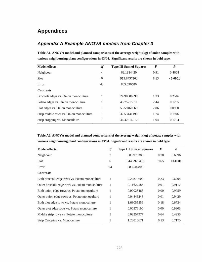
225
Appendices
Appendix A Example ANOVA models from Chapter 3
Table A1. ANOVA model and planned comparisons of the average weight (kg) of onion samples with
various neighbouring plant configurations in 03/04. Significant results are shown in bold type.
Model effects df Type III Sum of Squares F P
Neighbour 4 68.1884420 0.91 0.4668
Plot 6 913.8437163 8.13 <0.0001
Error 43 805.690586
Contrasts
Broccoli edges vs. Onion monoculture 1 24.98006990 1.33 0.2546
Potato edges vs. Onion monoculture 1 45.75715611 2.44 0.1255
Plot edges vs. Onion monoculture 1 53.59460069 2.86 0.0980
Strip middle rows vs. Onion monoculture 1 32.53441198 1.74 0.1946
Strip cropping vs. Monoculture 1 36.42516012 1.94 0.1704
Table A2. ANOVA model and planned comparisons of the average weight (kg) of potato samples with
various neighbouring plant configurations in 03/04. Significant results are shown in bold type.
Model effects df Type III Sum of Squares F P
Neighbour 7 50.9973388 0.78 0.6096
Plot 6 544.2923458 9.65 <0.0001
Error 94 883.502800
Contrasts
Both broccoli edge rows vs. Potato monoculture 1 2.20379609 0.23 0.6294
Outer broccoli edge rows vs. Potato monoculture 1 0.11627586 0.01 0.9117
Both onion edge rows vs. Potato monoculture 1 0.00025463 0.00 0.9959
Outer onion edge rows vs. Potato monoculture 1 0.04846243 0.01 0.9429
Both plot edge rows vs. Potato monoculture 1 1.68055556 0.18 0.6734
Outer plot edge rows vs. Potato monoculture 1 0.00576190 0.00 0.9803
Middle strip rows vs. Potato monoculture 1 6.02257977 0.64 0.4255
Strip Cropping vs. Monoculture 1 1.23816671 0.13 0.7175
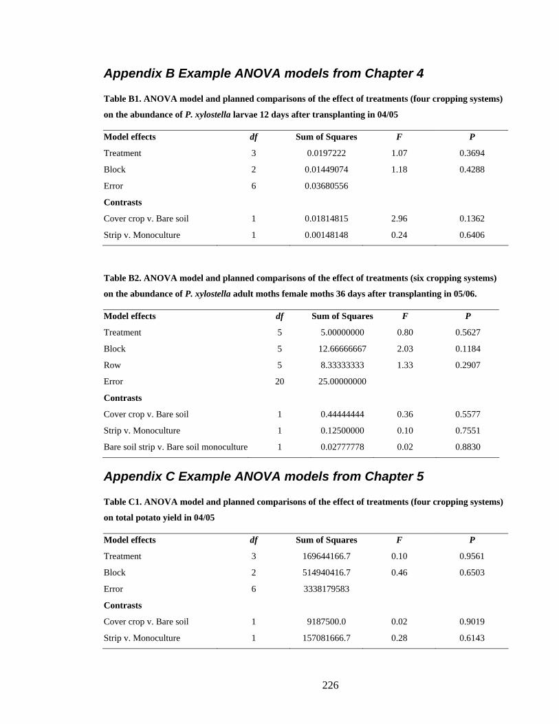
226
Appendix B Example ANOVA models from Chapter 4
Table B1. ANOVA model and planned comparisons of the effect of treatments (four cropping systems)
on the abundance of P. xylostella larvae 12 days after transplanting in 04/05
Model effects df Sum of Squares F P
Treatment 3 0.0197222 1.07 0.3694
Block 2 0.01449074 1.18 0.4288
Error 6 0.03680556
Contrasts
Cover crop v. Bare soil 1 0.01814815 2.96 0.1362
Strip v. Monoculture 1 0.00148148 0.24 0.6406
Table B2. ANOVA model and planned comparisons of the effect of treatments (six cropping systems)
on the abundance of P. xylostella adult moths female moths 36 days after transplanting in 05/06.
Model effects df Sum of Squares F P
Treatment 5 5.00000000 0.80 0.5627
Block 5 12.66666667 2.03 0.1184
Row 5 8.33333333 1.33 0.2907
Error 20 25.00000000
Contrasts
Cover crop v. Bare soil 1 0.44444444 0.36 0.5577
Strip v. Monoculture 1 0.12500000 0.10 0.7551
Bare soil strip v. Bare soil monoculture 1 0.02777778 0.02 0.8830
Appendix C Example ANOVA models from Chapter 5
Table C1. ANOVA model and planned comparisons of the effect of treatments (four cropping systems)
on total potato yield in 04/05
Model effects df Sum of Squares F P
Treatment 3 169644166.7 0.10 0.9561
Block 2 514940416.7 0.46 0.6503
Error 6 3338179583
Contrasts
Cover crop v. Bare soil 1 9187500.0 0.02 0.9019
Strip v. Monoculture 1 157081666.7 0.28 0.6143
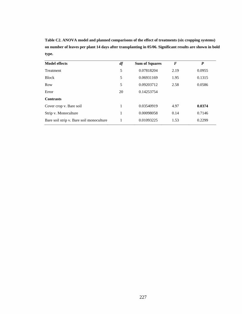
227
Table C2. ANOVA model and planned comparisons of the effect of treatments (six cropping systems)
on number of leaves per plant 14 days after transplanting in 05/06. Significant results are shown in bold
type.
Model effects df Sum of Squares F P
Treatment 5 0.07818204 2.19 0.0955
Block 5 0.06931169 1.95 0.1315
Row 5 0.09203712 2.58 0.0586
Error 20 0.14253754
Contrasts
Cover crop v. Bare soil 1 0.03540919 4.97 0.0374
Strip v. Monoculture 1 0.00098058 0.14 0.7146
Bare soil strip v. Bare soil monoculture 1 0.01093225 1.53 0.2299