Embed Size (px)
Citation preview

The Impacts of Asymmetric Information and Short
Sales on the Illiquidity Risk Premium in the Stock
Option Market
Chuang-Chang Chang, Zih-Ying Lin and Yaw-Huei Wang
____________________________________________________________________
ABSTRACT
The illiquidity risk premium hypothesis implies the existence of a positive
relationship between illiquidity in the option markets and option returns. Based upon
numerous studies within the extant literature examining the roles of informed traders
in the option markets, we explore the ways in which asymmetric information and
short sales can affect the illiquidity risk premium hypothesis. Our findings reveal
that the illiquidity risk premium is higher for the options of those firms with higher
information asymmetry, as well as those firms with higher short sales demand or
supply. These results are found to be particularly robust for short-term and/or OTM
contracts.
Keywords: Information asymmetry; Short sales; Short-sales constraints;
Informed traders; Option illiquidity premium.
JEL Classification: G14.
Chuang-Chang Chang and Zih-Ying Lin are collocated at the Department of Finance, National
Central University, Taiwan; Yaw-Huei Wang (the corresponding author) is at the Department of
Finance, National Taiwan University, Taiwan. Address for correspondence: Department of Finance,
National Taiwan University, No. 1 Roosevelt Road, Section 4, Taipei 106, Taiwan, ROC; Tel:
886-2-3366-1092; email: [email protected]. The authors are extremely grateful for the helpful
comments provided by Ji-Chai Lin, Hung-Neng Lai and Tzu-Hsiang Liao and also to the Ministry of
Science and Technology of Taiwan for the financial support provided for this study. (Zih-Ying Lin
will present the paper and email address is [email protected])
2
1. INTRODUCTION
Numerous studies have explored the relationship between illiquidity and expected
returns within the financial markets, including the stock, bond and derivative
markets. These studies have generally identified the existence of a positive
relationship between illiquidity and expected returns in the stock and bond markets.1
However, stocks and bonds are positive net supply assets, whereas derivatives are
traded with a zero net supply; thus, in some studies, the focus is shifted to the
associations between illiquidity and the expected returns on derivatives.
Bongaerts, De Jong and Driessen (2011) demonstrated that when investors with
short positions in zero net supply assets are taken into consideration, the illiquidity
premium could actually be zero, positive or negative; indeed, Deuskar, Gupta and
Subramanyam (2011) and Bongaerts et al. (2011) respectively found negative
illiquidity premiums in the credit default swap market and the interest rate derivative
market, whilst Christoffersen, Goyenko, Jaconbs and Karoui (2014) found a positive
relationship in the stock option market. Such inconsistencies within the extant
literature motivate us to further investigate the factors potentially affecting the
illiquidity risk premium in the stock option market.
1 The impact of stock illiquidity on expected stock returns was examined by Amihud and Mendelson
(1986, 1989), Amihud (2002), Pastor and Stambaugh (2003) and Acharya and Pedersen (2005);
Amihud and Mendelson (1991), Longstaff (2004) and Lin, Wang and Wu (2011) further noted that
bond illiquidity was related to ex-post bond returns.

3
As compared to trading in the underlying assets, option trading involves lower
transaction costs and provides higher leverage; thus, informed traders may choose to
trade in options in order to take advantage of their private information. As suggested
by Easley, O’Hara and Srinivas (1998), in order to earn profits, informed traders
with private information are more likely to trade in the option markets when the
option liquidity level is satisfactory and information asymmetry in the stock market
is high. Of particular significance is the fact that options can be used as a device for
circumventing the short-sale constraints in the stock market.
Many of the prior related studies, such as Manaster and Rendleman (1982) and
Sheikh and Ronn (1994), indicate that information is reflected in the option markets
prior to being reflected in the underlying stock markets, whilst Diamond and
Verrecchia (1987) suggested that informed traders with unfavorable information on
the underlying stocks will prefer to trade in the option markets. Furthermore,
following the demonstration by Vayanos and Wang (2012) of the ways in which
information asymmetry and imperfect competition affect liquidity and asset prices,
we posit that the involvement of informed traders may well play an important role in
the determination of the illiquidity risk premium in the option markets.
Whilst a number of studies have undertaken theoretical explorations of the ways
in which the existence of informed trading may affect the general risk premium, such

4
studies have reported quite mixed findings. For example, although both Leland (1992)
and Wang (1993) suggested that the existence of informed traders causes information
asymmetry and thus lowers the cost of capital for a firm, a number of other studies
have subsequently concluded that information asymmetry actually increases such
capital costs.2
From their examination of the differences in the composition of public and
private information, Easley and O’Hara (2004) noted that uninformed traders would
tend to demand a greater risk premium when trading with informed traders, since they
recognize the existence of an informational disadvantage, and hence, will tend to hold
fewer assets. This will ultimately drive down the prices of those securities with high
levels of private information (or information asymmetry), thereby leading to an
increase in the cost of capital for these firms.
These empirical findings suggest that private information induces a new form of
systematic risk, and that in equilibrium investors require compensation for taking such
risk. Thus, it seems natural to question whether the involvement of informed traders
changes the positive association between option illiquidity and expected option returns;
indeed, several related studies have documented the influence of information
asymmetry on the future dynamics of asset prices, with particular focus on the links
2 See O’Hara (2003), Easley and O’Hara (2004) and Hughes, Liu and Liu (2007).

5
between information asymmetry and subsequent stock returns.
For example, Pan and Poteshman (2006) found that stocks with low put-call
ratios outperformed stocks with high put-call ratios, with the predictability of stock
returns being higher for those stocks with high concentrations of informed traders.
Furthermore, using volatility spreads to predict stock returns based upon various
types of informational circumstances, Atilgan (2014) found that the predictability of
stock returns was stronger during major information events. Thus, our initial
objective in the present study is to examine whether the level of information
asymmetry plays an important role in the determination of the illiquidity risk
premium across firms in the option markets.
In addition to the level of information asymmetry, both short sales demand and
supply are also found to have impacts on trading by informed traders. On the
demand side, it was noted by Figlewski and Webb (1993) that the level of short
interest in the underlying stock can significantly affect the option prices of the stock;
thus, they argued that short selling was undertaken primarily by market professionals
who are also be likely to be informed traders.3 On the supply side, several studies
3 Since short selling is undertaken primarily by market professionals, who are also likely to be
informed traders, those stocks with high (low) levels of short interest provide a signal to the market that
the more informed traders expect the future prices of the stocks to fall (rise). Asquith and Meulbroek
(1995) also found that stocks with high short interest in one month tended to underperform in the
subsequent month, with their result suggesting that short interest is a bearish indicator conveying
negative information. Desai, Ramesh, Thiagarajan and Balachandran (2002) demonstrated that after
controlling for market size, book-to-market and momentum factors, firms with high levels of short
interest had significantly negative abnormal returns.

6
have demonstrated that short-sales constraints in the stock market affect trading
activities in the option market, with Hu (2014), for example, recently noting that
option trading is often considered to be an effective method of mitigating short-sales
constraints, and thus, conveying more information for those firms with greater
short-sales constraints.4 Our second objective is therefore to examine whether the
demand and supply levels of short sales have impacts on the illiquidity risk premium
across firms in the option markets.
Our empirical analysis involves the use of the ‘information asymmetry index’
(ASY-INDEX) and the ‘probability of informed trading’ (PIN) to measure
information asymmetry and the levels of short interest and institutional ownership in
a stock to respectively measure the demand and supply for short sales.5 Our
findings based upon US listed stocks and options are summarized as follows.
Firstly, we present evidence to show that the level of information asymmetry
has significant impacts on the option illiquidity risk premium across different firms,
particularly in the case of call options. The positive relationship that exists between
4 Examples include Diamond and Verrecchia (1987), Figlewski and Webb (1993) and Johnson and So
(2012). Informed traders with negative information could trade in the option market as an alternative to
short selling, especially when stocks are more difficult to sell short in the stock market. 5 Following Drobetz, Grüninger and Hirschvogl (2010), we use the error in analyst forecasts, firm
size, R&D expenditure, Tobin’s Q and the number of analysts covering the firm to compile the
information asymmetry index. The measure of the ‘probability of informed trading’ (PIN), which was
developed based upon the model of Easley et al. (1998), can be used to capture informed trading in
the market; this is an updated version of the data used in Brown, Hillegeist and Lo (2004). Cremers
and Weinbaum (2010) and Atilgan (2014) also used this data to investigate the role of informed
trading in the markets.

7
option illiquidity and expected option returns is found to be increased in those cases
where there is a higher concentration of informed traders, a finding which is
consistent with that of Easley and O’Hara (2004).
Secondly, we find that an increase in short sales strengthens the positive
relationship between option illiquidity and expected option returns for call options,
whilst higher short interest weakens the negative relationship for put options. Whilst
uninformed traders will demand greater compensation when holding more call
options (Easley and O’Hara, 2004), when there is higher short interest, the
dissemination of information on prices will reduce the uncertainty in the put prices
thereby reducing the illiquidity premium (Wang, 1993).
Finally, we find that higher short-sales costs (low institutional ownership) tend
to strengthen the positive relationship between option illiquidity and expected option
returns for put options; the reason for this is that put options contain more
information when there are greater short-sales constraints on the stocks.
In summary, we provide evidence to show that information asymmetry and the
demand and supply of short sales are important factors in the determination of the
option illiquidity risk premium across firms; this is consistent with the argument put
forward by Easley and O’Hara (2004) that uninformed traders will demand a greater
risk premium when trading with informed traders. Our empirical results are also

8
found to be particularly robust for short-term OTM options, which is consistent with
the general belief that informed traders tend to prefer to use those contracts with
higher leverage, better liquidity or lower transaction costs in order to take advantage
of their private information.
In addition to confirming the findings of Christoffersen et al. (2014), we
contribute to the extant literature by introducing the influences of informed traders
on the determination of option prices. We also demonstrate that information
asymmetry and the demand and supply of short sales are important factors
influencing the illiquidity risk premium across different firms.
The remainder of this paper is organized as follows. Section 2 provides details
of our hypothesis development, followed in Section 3 by a description of the data
and empirical measures used in our study. The empirical methodology adopted for
our analysis is described in Section 4, with Section 5 subsequently presenting and
discussing the empirical results. Finally, the conclusions drawn from this study are
presented in Section 6.
2. HYPOTHESIS DEVELOPMENT
Using the component firms of the S&P 500 index, Christoffersen et al. (2014)
examined the ways in which option illiquidity affected expected option returns and
identified a positive relationship between these two factors, which is consistent with

9
the risk premium hypothesis proposed by Amihud (2002). However, in contrast to
spot assets with a positive net supply, given that derivatives are zero net supply
assets, certain factors may play important roles in determining the risk premium.
It has been noted in many of the prior studies, such as Manaster and Rendleman
(1982) and Sheikh and Ronn (1994), that information is reflected in the option
market more rapidly than in the corresponding stock market, thereby leading to the
suggestion that the option market is the preferred venue for informed traders to
realize their private information. Easley, O’Hara and Srinivas (1998) set up a market
microstructure model to demonstrate that informed traders preferred to trade in the
option markets when option liquidity was high; Easley and O’Hara (2004)
subsequently noted that uninformed investors will tend to demand a higher risk
premium when they are faced with informed traders in the market.
From their analysis of the ways in which information asymmetry and imperfect
competition affect liquidity and asset prices, Vayanos and Wang (2012) found a
positive relationship with expected returns under information asymmetry when the
illiquidity was measured using Kyle’s lambda. In other words, the involvement of
informed traders may well vary across different firms, with uninformed traders
requiring a higher risk premium when there are more informed traders in the market
in order to compensate for their informational disadvantage, thereby leading to a

10
higher level of information asymmetry.
Based upon the findings and theorems of the related studies referred to above,
we argue that the level of information asymmetry may influence the relationship
between option illiquidity and expected option returns. We expect to find an
increasingly positive relationship between option illiquidity and expected option
returns with the level of information asymmetry. Accordingly, we propose the first
of our hypotheses, as follows:
Hypothesis 1: The relationship between option illiquidity and expected option
returns will be more positive for firms with higher information
asymmetry.
Figlewski and Webb (1993) demonstrated that the significantly higher average
level of short interest with ‘optionable’ stocks (those stocks selected as the
underlying asset of an option) provides support for the argument that option trading
facilitates short selling. They also found that short interest in the underlying stock
could significantly affect option prices and went on to suggest that short sales were
primarily undertaken by market professionals.
Diamond and Verrecchia (1987) had earlier indicated that speculative short
sellers were more likely to trade in the option markets (with a particular focus on
trading in put options) essentially because, on the one hand, such trading could

11
reduce their short sales costs, whilst on the other hand, it could increase their
leverage. These studies therefore seem to jointly suggest that the level of short
interest is positively related to the amount of informed trading, since short selling is
widely regarded as being carried out primarily by market professionals.
Given that informed traders prefer to trade in the option market when they have
access to private (especially negative) information, the level of short interest should
be positively related to the level of information asymmetry. As suggested by Easley
and O’Hara (2004), uninformed traders demand a greater risk premium when trading
with informed traders because compensation is required for their losses. Thus, if
uninformed traders hold more call options of those stocks with higher short interest,
they naturally assume greater risk as a direct result of their informational
disadvantage. Accordingly, investors holding more call options of those stocks with
higher short interest may require a greater risk premium. This leads to the
development of our second hypothesis, as follows:
Hypothesis 2: The relationship between option illiquidity and expected option
returns will be more positive for firms with higher short interest,
particularly in the case of call options.
In addition to the demand side of short sales explored by the studies referred to
above, the stock market supply side (short-sale constraints or short-sales costs) can

12
also affect trading activities in the option markets. Informed traders with negative
information could trade in the option market as an alternative to short selling,
particularly in those cases where the difficulty of engaging in short selling in the
stock market is high; that is to say, if there are higher levels of short-sales
constraints in the stock market, informed traders with negative information are more
likely to trade in the option market.6
Some of the prior studies using institutional ownership as a proxy for the
market supply of short interest have identified the existence of a negative
relationship between the level of institutional ownership and the difficulties involved
in engaging in short selling (see D’Avolio, 2002; Asquith, Pathak and Ritter, 2005).
Hu (2014) also found that the informational benefit of option trading was higher for
stocks with greater short-sales constraints.
Given that informed traders have incentive to buy put options to realize their
private negative information for firms with higher short-sales costs, uninformed
traders buying put options may assume greater levels of risk. We therefore consider
shorting supply to construct out third hypothesis, as follows:
Hypothesis 3: The relationship between option illiquidity and expected option
returns will be more positive for firms with lower institutional
ownership (higher short-sales costs), particularly in the case of
6 See Diamond and Verrecchia (1987), Figlewski and Webb (1993), Johnson and So (2012), Hu (2014).

13
put options.
3. DATA
The primary dataset adopted for this study includes stock option quotes and the
illiquidity measures of both stocks and options, with the measures of both
information asymmetry and the demand and supply of short sales also being utilized
in our empirical analysis. The sample period adopted for this study runs from
January 1996 to December 2007.7
3.1 Stock Option Quotes and Computation of Option Returns
The stock options data were collected from Option Metrics, with the dataset including
daily closing bid and ask quotes, implied volatility levels and the deltas of all stock
options listed in the US exchanges. As regards time to maturity, short-term options are
defined as those with maturity periods ranging from 20 and 70 days, whilst long-term
options are those with maturity periods ranging from 71 and 180 days.
Following Bollen and Whaley (2004) and Driessen, Maenhout and Vilkov (2009),
we also adopt the option delta for our classification of moneyness in the present study.
The call (put) deltas for OTM options range from 0.125 to 0.375 (–0.375 to –0.125),
whilst those for ATM options range from 0.375 to 0.625(–0.625 to –0.375) and those
7 If the short-sales ban is taken into consideration, an unexpected bias may twist the analysis in the
present study; thus, the period after 2007 is not included in our sample period. This issue has been
noted in many of the prior related studies, such as Battalio and Schultz (2011), Autore, Billingsley
and Kovacs (2011), Grundy, Lim and Verwijmeren (2012) and Boehmer, Jones and Zhang (2013).

14
for ITM options range from 0.625 to 0.875 (–0.875 to –0.625).
Those option contracts which meet the following criteria are excluded from our
sample in order to deal with concerns regarding liquidity or reliability: (i) prices
violate the no-arbitrage conditions; (ii) ask price ≤ bid price; (iii) open interest is equal
to 0; (iv) price details are incomplete; (v) price < $3 and bid-ask spread < $0.05 or price
≥ $3 and bid-ask spread < $0.10.
Following Frazzini and Pedersen (2012) and Christoffersen et al. (2014), we
compute the daily delta-hedged returns of options as:
(1)
where is the daily raw return of option n and
is computed based
upon the Cox, Ross and Rubinstein (1979) binomial tree model allowing for early
exercise, given that all stock options are American style options. St is the price of the
underlying stock at time t and is the stock return computed from St and St+1.
All of the details on stock prices are obtained from CRSP.
Following Coval and Shumway (2001), we use the bid-ask midpoints to
compute the raw option return ) as the equally-weighted average of the daily
returns of all available options in each moneyness and maturity category. In other
words, the return of a particular category of a firm from t to t + 1 is defined as:

15
(2)
The corresponding delta-hedged return is then computed as:
(3)
where N is the number of available contracts in each category at time t with quotes
at time t + 1; and Ot(Kn, Tn ) is the mid-point quote of an option with strike price Kn
and maturity Tn.8
The summary statistics of the option returns across various maturity-moneyness
categories for call and put options are reported in Table 1. We first of all compute
the descriptive statistics for each firm and then take the cross-sectional averages of
these statistics, as a result of which we find that the returns of put options are
generally higher than those of call options. Returns on short-term options are more
volatile than returns on long-term options, especially for OTM contracts.
<Table 1 is inserted about here>
3.2 Stock and Option Illiquidity Measures
Using the data obtained from the high-frequency intraday ‘trade and quote’ (TAQ)
database, stock illiquidity is calculated in this study as the effective spread.9 The
8 We use the adjustment factor provided by Option Metrics for splits and other distribution events.
9 The same illiquidity measure has also been adopted in many of the prior related studies, including
Hasbrouck and Seppi (2001), Huberman and Halka (2001), Chordia, Roll and Subrahmanyam (2000;
2001) and Chordia, Sarkar and Subrahmanyam (2005).

16
effective spread is defined as:
(4)
where Pk is the price of the kth
trade; and Mk is the midpoint of the best bid and offer
prices at the time of the kth
trade.
The dollar-volume weighted average of all computed over all trades
during the day defines the daily effective spread of the stock, ILS, as follows:
(5)
where DolVolk refers to the dollar-volume computed as the product of the stock
price and the trading volume.
Similar to Cao and Wei (2010), we adopt the relative quoted bid-ask spread as
the measure of option illiquidity, which is computed from the end-of-day quoted bid
and ask prices provided by Ivy DB Option Metrics.10
For each contract, we compute
the daily relative quoted spread as:
(6)
where Ot(Kn, Tn ), OAt(Kn, Tn ) and OBt(Kn, Tn ) are the respective end of day closing
mid-point, ask and bid quotes for an option with strike price Kn and maturity Tn. It
should be noted that Ot(Kn, Tn ) = (OAt(Kn, Tn ) + OBt(Kn, Tn ))/2.
10
As suggested by Cao and Wei (2010), the dollar quoted bid-ask spread is not a good alternative
liquidity indicator because it is mainly driven by the maturity and moneyness of an option contract.

17
(7)
where N is the number of available contracts within the category at time t.
The summary statistics of the relative bid-ask spread illiquidity measures for all
firms are presented in Table 2. According to the option illiquidity (ILO), we find that
short-term contracts are more illiquid than long-term contracts for both call and put
options, with OTM contacts exhibiting the highest overall illiquidity.
<Table 2 is inserted about here>
3.3 Information Asymmetry Measures
Two measures of information asymmetry are adopted in this study. Firstly, following
Drobetz et al. (2010), we create an information asymmetry index with the exclusion
of those firms with a fiscal year not ending with the corresponding calendar year.
Secondly, we follow several of the prior related studies on informed trading to use
the ‘probability of informed trading’ (PIN) to measure information asymmetry.11
Various measures of information asymmetry have been introduced within the
prior empirical studies; for example, Vermaelen (1981) identified the tendency for a
reduction in information asymmetry with firm size, whilst Smith and Watts (1992)
discovered an increase in information asymmetry with growth opportunities.
Krishnaswami and Subramaniam (1999) indicated that information asymmetry was
11
See Easley et al. (1998) and Easley, Kiefer and O’Hara (1997; 2002).

18
reduced in line with the number of analysts tracing the firm, and went on to suggest
the use of analyst forecast errors as an effective measure for information asymmetry.
Finally, Aboody and Lev (2000) also found an increase in information asymmetry
with R&D expenditure.
For our first measure of information asymmetry in the present study, we follow
the method of Drobetz et al. (2010) to construct an information asymmetry index
(ASY-INDEX) based upon the various dimensions of the concepts described above.
These dimensions include analyst forecast errors,12
firm size, R&D expenditure,
Tobin’s Q and the number of analysts tracing the firm.13
The accounting data, which
is obtained from Compustat, includes R&D expenditure and total assets. Details on
the analyst forecasts and the number of tracking analysts are collected from I/B/E/S.
12
We use the following measure of analyst forecast errors: / , where EPSForecast is the earnings per share forecast, which is the average
of all forecasts for a firm provided by all analysts in November and December of the previous year.
The difference between actual and forecasted earnings per share is scaled by the median earnings per
share forecast. 13
Elton, Gruber and Gultekin (1984) noted that most of the forecast error in the last month of the fiscal
year could be explained by erroneous estimation of firm-specific factors. Diamond and Verrecchia
(1991) and Ozkan and Ozkan (2004) further indicated that large firms may be faced with less
information asymmetry essentially because they are more mature and have more transparent disclosure
policies; thus, they tend to receive more attention from the market. From their analysis of insider trading
gains in firms with high and low R&D expenditure, Aboody and Lev (2000) found that the insider gains
in R&D firms were larger than those in firms with no R&D, and provided evidence to show that R&D
was related to information asymmetry. Following the indication by Smith and Watts (1992) that
information asymmetry was more serious for firms with significant growth opportunities, McLaughlin,
Safieddine and Vasudevan (1998) used investment opportunities as a proxy for information asymmetry.
In the present study, we use Tobin’s Q, defined as the book value of assets minus the book value of
equity plus the market value of equity divided by the book value of assets, to measure growth
opportunities. Chang, Dasgupta and Hillary (2006) suggested that the greater the analyst cover of a firm,
the higher the information released to the public, and hence, the more limited the level of information
asymmetry; the number of analysts can therefore also be used to proxy for information asymmetry.
Brennan and Subrahmanyam (1995) argued that higher analyst coverage could reduce the adverse
selection costs, as measured by the inverse of market depth.

19
For our compilation of the index, we first of all calculate the annual quintile
ranking of a firm over all firms for each dimension of information asymmetry, with
a higher score indicating a higher level of information asymmetry; for instance, a
firm will be assigned a score of 5 (1) if it belongs in the smallest (largest) 20 per
cent of all firms in a given year. We then sum the ranks for all five dimensions of
information asymmetry, with the largest (smallest) value of the ASY-INDEX for
firms with the highest (lowest) level of information asymmetry being 25 (5). The
PIN is used as the second measure of information asymmetry in our analysis, with
the quarterly PIN estimates for the period from January 1996 to December 2006
having been obtained from Stephen Brown.
3.4 Short Sales Measures
One stream of the extant literature on short sales suggests that high short interest
ratios (shares sold short over shares outstanding) predicts low future returns,14
whilst an alternative stream indicates that short sales are dependent upon the
institutional ownership of the stock.15
We also follow Asquith et al. (2005) to consider both short sales demand and
supply so as to define the level of stocks to short sales. We follow Figlewski and
14
Examples include Figlewski (1981), Figlewski and Webb (1993), Senchack and Starks (1993),
Asquith and Meulbroek (1995) and Desai et al. (2002). 15
See D’Avolio (2002), Asquith et al. (2005) and Hu (2014).

20
Webb (1993) to use the short interest ratio as a proxy for short sales demand and as
suggested by D’Avolio (2002) and Asquith et al. (2005), we take institutional
ownership as the proxy for the market supply of short interest, since it has a negative
correlation with the difficulties involved in short selling.
The data on short interest are obtained from Compustat on the fifteenth day of
the month (or the nearest trading day if the fifteenth day is not a trading day), whilst
the institutional ownership data are obtained from 13-F filings. The descriptive
statistics on the information asymmetry measures, comprising of the means, medians,
standard deviations and 10%, 50% and 90% percentiles, are reported in Table 3.
<Table 3 is inserted about here>
4. METHODOLOGY
Christoffersen et al. (2014) identified a positive relationship between option
illiquidity and expected option returns, attributing this result to the option illiquidity
premium. However, given that derivatives are zero net supply assets, they are more
complicated than assets with positive net supplies; therefore, for our examination of
the ways in which information asymmetry and short sales affect the positive
relationship identified by Christoffersen et al. (2014), we modify the regression
model adopted in their study to consider the effect of information asymmetry in

21
order to test Hypothesis 1, as follows:16
(8)
where are the delta-hedge option returns;
refers to the option illiquidity
and denotes the stock illiquidity; DummyAsy.Info. is a dummy variable which
takes the value of 1 if the ASY-INDEX for stock i is ranked in the top 20 per cent;
otherwise 0; and σi,t denotes the historical volatility estimated using the daily stock
returns from the GARCH(1,1) model.
As suggested by Duan and Wei (2009), bi,t is the square root of the R2 from
running the daily OLS regressions of the excess stock returns on the four factors
proposed by Fama and French (1993) and Carhart (1997), with a one-year rolling
window. Furthermore, we follow both Dennis and Mayhew (2002) and Duan and
Wei (2009) to control for size and leverage; sizei,t is the natural logarithm of the
market capitalization of the firm; and levi,t is defined as the sum of long-term debt
and the par value of the preferred stock, divided by the sum of long-term debt, the
par value of the preferred stock and the market value of equity.
We expect to find that if the illiquidity premium hypothesis holds, then β2 will
16
In order to run a reliable cross-sectional regression, there is a requirement of a minimum of 30
firm observations for each time t.

22
be positive, and if investors require a higher risk premium for the options of stocks
with higher levels of information asymmetry, then β4 will be significantly positive.
Based upon the replication argument proposed by Leland (1985) and Boyle and
Vorst (1992), we also expect to find that β3 will be positive.17
When using the PIN as an alternative proxy for information asymmetry, the
terms with DummyAsy.Info. are not included in the regression model; instead, we first
of all group the firms based on their quarterly PIN levels into the three categories of
low (<30%), mid (30-70%) and high (>70%), and then run the cross-sectional
regression model without the dummy term for the returns of options across various
moneyness-maturity categories in order to examine the significance of the mean of
the β2 coefficients for each category.
As regards the short sales demand side, we follow Figlewski and Webb (1993)
to use the relative short interest (that is, the number of shares sold short divided by
the total outstanding shares of the firm) as the measure of the annual average short
interest. For the supply side, we follow Asquith et al. (2005) and Hu (2014) to
consider institutional ownership as the proxy for short-sales constraints (short-sales
costs) and then rewrite the regression models, as shown below, to respectively test
17
An option can be replicated by trading the underlying asset and a risk free bond in a frictionless and
complete-market model; however, this is not the case, given the existence of liquidity risk. Market
makers have net long positions in the equity option markets, and hence, need to create a synthetic short
option using the underlying stock. This will lead to a reduction in the price that market makers receive
from shorting the synthetic option with the illiquidity of the stock market, thereby reducing the option
price.

23
Hypotheses 2 and 3:
(9)
and
(10)
where the DummyRSI. variable takes the value of 1 if the relative short interest for
stock i is ranked in the top 20 per cent; otherwise 0; and the Dummyop. variable takes
the value of 1 if the institutional ownership for stock i is ranked in the bottom 20 per
cent; otherwise 0. Similarly, if Hypothesis 2 (3) holds, then we would expect to find
that β4 will be significantly positive, particularly for call (put) options.
5. EMPIRICAL RESULTS
5.1 Preliminary Results
Prior to using our regression models to formally test for the impacts of information
asymmetry and short sales on the illiquidity risk premium, we provide some
preliminary evidence on the existence of the illiquidity risk premium in the option
markets. We short the stocks according to their previous-day illiquidity measures
and form three groups of firms in the categories of low (<30%), mid (30-70%) and

24
high (>70%) illiquidity for each day. We then calculate the delta hedge returns of
options for each group of firms across various moneyness-maturity categories. The
average option returns for all categories are reported in Table 4.
<Table 4 is inserted about here>
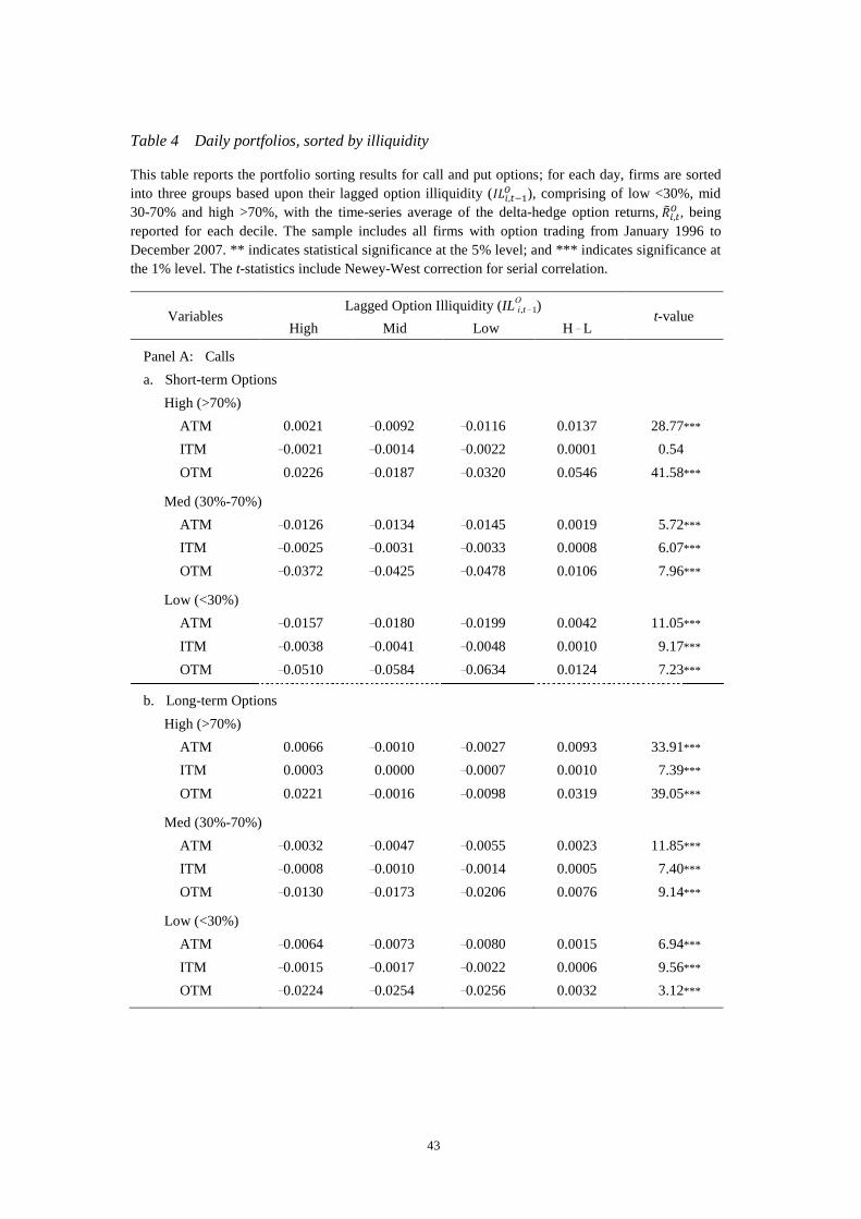
Regardless of which moneyness or maturity is considered, the average return
for the high-illiquidity group is always found to be higher than that for the low-
illiquidity group, with almost all of the differences being significant at the 1% level.
In other words, the average option returns are positively associated with the option
illiquidity levels; this is in line with the findings of Christoffersen et al. (2014) and
confirms the existence of the illiquidity risk premium in the option markets
5.2 Results on Information Asymmetry
In order to test Hypothesis 1, we first of all run the cross-sectional regression model
specified in Equation (8) for each day and then take the time-series averages of the
regression coefficients. We report the results based upon the information asymmetry
index (ASY-INDEX) in Table 5, with Newey and West (1987) adjusted t-statistics.
As shown in Panel A, the overall results on call options are found to be consistent
across all moneyness and maturity groups.
<Table 5 is inserted about here>
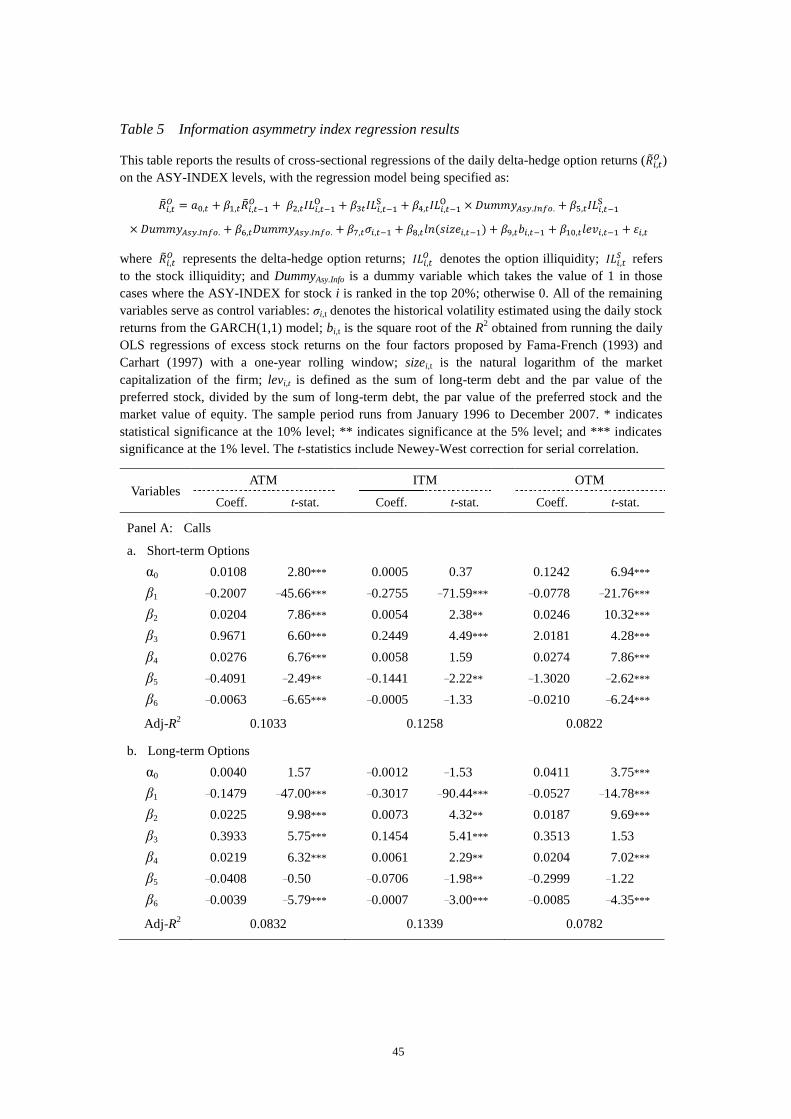
The positive significance of β2 is in line with the illiquidity risk premium

25
hypothesis, which is again consistent with the findings of Christoffersen et al. (2014).
The positive β3 provides support for the option replication argument proposed by
Leland (1985) and Boyle and Vorst (1992), although it is found to be insignificant
for long-term OTM call options. The β4 coefficient is found to positively significant
at the 5% level for all groups, with the one exception of short-term ITM call options,
thereby confirming Hypothesis 1. In other words, our regression results on call
options strongly indicate that the higher the level of information asymmetry, the
higher the illiquidity risk premium.
Furthermore, the information asymmetry effect is found to be particularly
strong for short-term call options, essentially because β2 + β4 is higher for short-term
contracts than long-term contracts. This finding could be attributable to the fact that
informed traders are more likely to trade in short-term contracts, as opposed to
long-term contracts, so that they can take advantage of certain aspects of the former,
such as higher leverage and liquidity.
By contrast, as shown in Panel B, the results from put options are less
convincing since the β4 coefficient is found to be positively significant only for
OTM options, which could be attributable to uninformed investors tending to view
put options as insurance against existing long positions on the underlying asset,

26
whilst also choosing not to speculate on negative news.18
Although the effect of
information asymmetry is less robust for put options, full support is still provided for
the illiquidity risk premium hypothesis since all of the β2 coefficients are found to be
positively significant at the 1% level.
Our finding that the effect of the impact is particularly pronounced for OTM
contracts, which are not dependent on call/put or short-/long-term contracts, is of
some importance, since this finding suggests that informed traders prefer to trade in
OTM options in order to take advantage of their private information, and thus,
uninformed traders require a higher risk premium when trading in this group of
contracts to compensate for the risk that they face due to their informational
disadvantage.
The empirical results obtained from PIN, the alternative proxy for information
asymmetry, are shown in Table 6. Since the PIN dataset is obtained with quarterly
frequency, we run the cross-sectional regression model specified in Equation (8)
without the information asymmetry dummy variable for each day on the returns of
options across various moneyness-maturity categories for the three groups of firms
grouped by their PIN levels. The means of the β2 coefficients and their t-statistics
are reported in Table 6.
18
Several prior studies, including Bates (1996), Pan (2002) and Bakshi Kapadia and Madan (2003)
have shown that hedging demand drives the pricing of put options more than the pricing of call options.

27
<Table 6 is inserted about here>
The results based upon the PIN levels are generally consistent with those based
upon the ASY-INDEX, with strong support being provided for the illiquidity risk
premium hypothesis since virtually all of the β2 coefficients are found to be
positively significant at the 1% level. Furthermore, the β2 coefficients of the higher
PIN groups are found to be larger than those of the lower PIN groups for the
majority of the moneyness-maturity categories, a finding which is particularly robust
for OTM (call and put) contracts.
In summary, both the ASY-INDEX and PIN results indicate that uninformed
traders require a higher illiquidity risk premium for the options of firms with higher
levels of information asymmetry, thereby confirming Hypothesis 1.
5.3 Results on Demand and Supply of Short Sales
Following Asquith et al. (2005), we consider the demand-side and supply-side
measures of short sales in order to investigate their overall impact on the illiquidity
risk premium hypothesis when informed traders are in possession of negative private
information. The results from the demand-side measure for short interest are shown
in Table 7.
<Table 7 is inserted about here>
For call options, with the exception of ITM contracts, we find that the

28
illiquidity risk premium is higher when there is higher short selling of stocks,
essentially because all of the β4 coefficients are found to be positively significant at
the 5% level; however, there is no clear pattern for put options. In summary, the
effect of the demand of short sales on the illiquidity risk premium is particularly
high for OTM call options, with these findings being largely consistent with
Hypothesis 2, as well as the ASY-INDEX and PIN results.
A higher level of short interest indicates a bearish prospect for the firm. Given
unfavorable information on the underlying stocks, informed traders will not only
short sell the stocks, but also buy put options, since trading in the latter attracts
lower transaction costs, whilst providing higher leverage. Under such circumstances,
uninformed traders buying more call options will require a higher risk premium as
they are more likely to lose out to informed traders who may trade more put options,
an argument which is consistent with that of Easley and O’Hara (2004).
Conversely, the short interest level signals the release of negative information,
which lowers the uncertainty of trading in put options. Consequently, investors
trading in put options will not demand a higher illiquidity risk premium when the
level of short interest in the underlying stock is higher. For most of the moneyness-
maturity categories, we even find a negative β4 coefficient, which is consistent with
the argument of Wang (1993), that the illiquidity risk premium for put options will

29
be lower when there is greater short interest in the underlying stock.
The results on the impact of the supply-side measure (short-sales constraints or
short-sales costs) on the illiquidity risk premium are shown in Table 8. Although
there are no significant findings for call options, for put options, almost all of the β4
coefficients are found to be positive, with significance at the 1% level, for OTM
contracts. In contrast to our earlier findings using other measures, the findings on
short-sales constraints suggest that uninformed investors trading in put options will
tend to demand a higher illiquidity risk premium for those stocks with higher
short-sales constraints.
<Table 8 is inserted about here>
The option market can be used as a device for circumventing short-sales
constraints in the stock market. For those stocks with greater short-sales constraints,
informed traders will inevitably choose to trade in put options when they are in
possession of private negative information. Therefore, uninformed traders buying
put options on those stocks with high short-sales constraints will require a higher
illiquidity risk premium since the risk arising from their informational disadvantage
is higher. Although uninformed traders may realize that the put option market is a
channel for informed traders to take advantage of their private negative information,
they do not know when they will choose to do so; however, this is not the case for

30
call options. These findings are generally consistent with Hypothesis 3.
In summary, we provide evidence to show that for both call and put options,
information asymmetry and short sales have significant impacts on the illiquidity
premium. Our findings reveal that information asymmetry and short interest
(short-sale costs) are positively associated with the option illiquidity risk premium,
particularly for call (put) options. Furthermore, these results are found to be
especially robust for short-term or OTM option contracts, a finding which is
consistent with the common belief that informed traders are more likely to trade in
these contracts in order to realize their private information.
6. CONCLUSIONS
Based on the extant literature on the roles of informed traders in the option markets,
we extend the work of Christoffersen et al. (2014) to examine the ways in which
information asymmetry and short sales affect the option illiquidity risk premium. In
addition to using the two measures of information asymmetry (ASY-INDEX and
PIN), we also use the demand-side and supply-side measures of short sales (short
interest and short-sales constraints) in order to examine their impacts on the
relationship between option returns and option illiquidity.
Our findings reveal that both information asymmetry and short sales have
significantly positive impacts on the option illiquidity risk premium, with our

31
empirical results being found to be particularly robust for short-term contracts.
These findings are also consistent with the argument put forward by Easley and
O’Hara (2004) that uninformed traders will demand a greater risk premium when
trading with informed traders.
In addition to confirming the findings of Christoffersen et al. (2014), we also
contribute to the extant literature by introducing the influences of informed traders
on the determination of option prices and documenting that information asymmetry
and the demand and supply of short sales are important factors influencing the
illiquidity risk premium across different firms.

32
REFERENCES
Aboody, D. and B. Lev (2000), ‘Information Asymmetry, R&D and Insider Gains’,
Journal of Finance, 55: 2747-66.
Acharya, V. and L. Pedersen (2005), ‘Asset Pricing with Liquidity Risk’, Journal of
Financial Economics, 77: 375-410.
Amihud, Y. and H. Mendelson (1986), ‘Asset Pricing and the Bid-Ask Spread’,
Journal of Financial Economics, 17: 223-49.
Amihud, Y. and H. Mendelson (1989), ‘The Effect of Beta, Bid-Ask Spread,
Residual Risk and Size on Stock Returns’, Journal of Finance, 2: 479-86.
Amihud, Y. and H. Mendelson (1991), ‘Liquidity, Maturity, and the Yields on US
Treasury Securities’, Journal of Finance, 46: 1411-25.
Amihud, Y. (2002), ‘Illiquidity and Stock Returns: Cross-section and Time-series
Effects’, Journal of Financial Markets, 5: 31-56.
Asquith, P. and L. Meulbroek (1995), ‘An Empirical Investigation of Short Interest’,
Working paper, MIT.
Asquith, P., P.A. Pathak and J.R. Ritter (2005), ‘Short Interest, Institutional Ownership
and Stock Returns’, Journal of Financial Economics, 78: 243-76.
Atilgan, Y. (2014), ‘Volatility Spreads and Earnings Announcement Returns’, Journal
of Banking Finance, 38: 205-15.
Autore, D.M., R.S. Billingsley and T. Kovacs (2011), ‘The 2008 Short Sale Ban:
Liquidity, Dispersion of Opinion and the Cross-section of Returns of US
Financial Stocks’, Journal of Banking and Finance, 35: 2252-66.

33
Bakshi, G., N. Kapadia and D. Madan (2003), ‘Stock Return Characteristics, Skew
Laws and Differential Pricing of Individual Equity Options’, Review of
Financial Studies, 16: 101-43.
Bates, D. (1996), ‘Jumps and Stochastic Volatility: Exchange Rate Processes Implicit
in Deutsche Mark Options’, Review of Financial Studies, 9: 69-107.
Battalio, R. and P. Schultz (2011), ‘Regulatory Uncertainty and Market Liquidity:
The 2008 Short Sale Ban’s Impact on Equity Option Markets’, Journal of
Finance, 66: 2013-53.
Boehmer, E., C. Jones and X. Zhang (2013), ‘Shackling Short Sellers: The 2008
Shorting Ban’, Review of Financial Studies, 26: 1363-1400.
Bollen, N. and R. Whaley (2004), ‘Does Net Buying Pressure Affect the Shape of
Implied Volatility Functions?’, Journal of Finance, 59: 711-53.
Bongaerts, D., F. De Jong and J. Driessen (2011), ‘Derivative Pricing with Liquidity
Risk: Theory and Evidence from the Credit Default Swap Market’, Journal of
Finance, 66: 203-40.
Boyle, P. and T. Vorst (1992), ‘Option Replication in Discrete Time with Transaction
Costs’, Journal of Finance, 47: 271-93.
Brennan, M. and A. Subrahmanyam (1995), ‘Investment Analysis and Price Formation
in Securities Markets’, Journal of Financial Economics, 38: 361-81.
Brown, S., S.A. Hillegeist and K. Lo (2004), ‘Conference Calls and Information
Asymmetry’, Journal of Accounting and Economics, 37: 343-66.

34
Cao, M. and J. Wei (2010), ‘Commonality in Liquidity: Evidence from the Option
Market’, Journal of Financial Markets, 13: 20-48.
Carhart, M. (1997), ‘On Persistence of Mutual Fund Performance’, Journal of
Finance, 52: 57-82.
Chang, X., S. Dasgupta and G. Hillary (2006), ‘Analysts Coverage and Financing
Decisions’, Journal of Finance, 61: 3009-48.
Chordia, T., R. Roll and A. Subrahmanyam (2000), ‘Commonality in Liquidity’,
Journal of Financial Economics, 56: 3-28.
Chordia, T., R. Roll and A. Subrahmanyam (2001),’ Market Liquidity and Trading
Activity’, Journal of Finance, 56: 501-30.
Chordia, T., A. Sarkar and A. Subrahmanyam (2005), ‘An Empirical Analysis of
Stock and Bond Market Liquidity’, Review of Financial Studies, 18: 85-129.
Christoffersen, P., R. Goyenko, K. Jacobs and M. Karoui (2014), ‘Illiquidity Premia
in Equity Options Market’, Working Paper, University of Toronto.
Coval, J. and T. Shumway (2001), ‘Expected Option Returns’, Journal of Finance,
56: 983-1009.
Cox, J., S. Ross and M. Rubinstein (1979), ‘Option Pricing: A Simplified Approach’,
Journal of Financial Economics, 7: 229-63.
Cremers, M. and D. Weinbaum (2010), ‘Deviations from Put-Call Parity and Stock
Return Predictability’, Journal of Financial and Quantitative Analysis, 45:
335-67.

35
D’Avolio, G. (2002), ‘The Market for Borrowing Stock’, Journal of Financial
Economics, 66: 271-306.
Dennis, P. and S. Mayhew (2002), ‘Risk-neutral Skewness: Evidence from Stock
Options’, Journal of Financial and Quantitative Analysis, 37: 471-93.
Desai, H., K. Ramesh, S.R. Thiagarajan and B.V. Balachandran (2002), ‘An
Investigation of the Informational Role of Short Interest in the Nasdaq Market’,
Journal of Finance, 57: 2263-87.
Deuskar, P., A. Gupta and M. Subrahmanyam (2011), ‘Liquidity Effect in OTC
Options Markets: Premium or Discount?’, Journal of Financial Markets, 14:
127-60.
Diamond, D.W. and R.E. Verrecchia (1987), ‘Constraints on Short-Selling and Asset
Price Adjustment to Private Information’, Journal of Financial Economics, 18:
277-312.
Diamond, D.W. and R.E. Verrecchia (1991), ‘Disclosure, Liquidity and the Cost of
Capital’, Journal of Finance, 46: 1325-59.
Driessen, J., P. Maenhout and G. Vilkov (2009), ‘The Price of Correlation Risk:
Evidence from Equity Options’, Journal of Finance, 64: 1377-406.
Drobetz, W., M.C. Grüninger and S. Hirschvogl (2010), ‘Information Asymmetry
and the Value of Cash’, Journal of Banking and Finance, 34: 2168-84.
Duan, J.C. and J. Wei (2009), ‘Systematic Risk and the Price Structure of Individual
Equity Options’, Review of Financial Studies, 22: 1981-2006.

36
Easley, D., S. Hvidkjaer and M. O’Hara (2002), ‘Is Information Risk a Determinant
of Asset Returns?’, Journal of Finance, 57: 2185-221.
Easley, D., N. Kiefer and M. O’Hara (1997), ‘One Day in the Life of a Very
Common Stock’, Review of Financial Studies, 10: 805-35.
Easley, D., M. O’Hara and P. Srinivas (1998), ‘Option Volume and Stock Prices:
Evidence on Where Informed Traders Trade’, Journal of Finance, 53: 432-65.
Easley, D. and M. O’Hara (2004), ‘Information and the Cost of Capital’, Journal of
Finance, 59: 1553-83.
Elton, E.J., M.J. Gruber and M.N. Gultekin (1984), ‘Professional Expectations: Accuracy
and Diagnosis of Errors’, Journal of Financial & Quantitative Analysis, 19: 351-63.
Fama, E. and K. French (1993), ‘Common Risk Factors in the Returns on Stocks and
Bonds’, Journal of Financial Economics, 33: 3-56.
Figlewski, S. (1981), ‘The Information Effects of Restrictions on Short Sales: Some
Empirical Evidence’, Journal of Financial and Quantitative Analysis, 16: 463-76.
Figlewski, S. and G.P. Webb (1993), ‘Options, Short Sales and Market
Completeness’, Journal of Finance, 48: 761-77.
Frazzini, A. and L.H. Pedersen (2012), ‘Embedded Leverage’, Working Paper,
University of New York.
Grundy, B.D., B. Lim and P. Verwijmeren (2012), ‘Do Options Markets Undo
Restrictions on Short Sales? Evidence from the 2008 Short-Sale Ban’, Journal
of Financial Economics, 106: 331-48.

37
Hasbrouck, J. and D. Seppi (2001), ‘Common Factors in Prices, Order Flows and
Liquidity’, Journal of Financial Economics, 59: 383-411.
Hu, J.F. (2014), ‘Does Option Trading Convey Stock Price Information?’, Journal
of Financial Economics, 111: 625-45.
Huberman, G. and D. Halka (2001), ‘Systematic Liquidity’, Journal of Financial
Research, 2: 161-78.
Hughes, J., J. Liu and J. Liu (2007), ‘Information, Diversification and the Cost of
Capital’, Accounting Review, 82: 705-29.
Johnson, T.L. and E.C. So (2012), ‘The Option to Stock Volume Ratio and Future
Returns’, Journal of Financial Economics, 106: 262-86.
Krishnaswami, S. and V. Subramaniam (1999), ‘Information Asymmetry, Valuation
and the Corporate Spin-off Decision’, Journal of Financial Economics, 53:
73-112.
Kyle, A. (1985), ‘Continuous Auctions and Insider Trading’, Econometrica, 6:
1315-36.
Leland, H. (1985), ‘Option Pricing and Replication with Transaction Costs’, Journal
of Finance, 40: 1283-301.
Leland, H. (1992), ‘Insider Trading: Should It Be Prohibited?’, Journal of Political
Economy, 100: 859-87.
Lin, H., J. Wang and C. Wu (2011), ‘Liquidity Risk and Expected Corporate Bond
Returns’, Journal of Financial Economics, 99: 628-50.

38
Longstaff, F. (2004), ‘The Flight-to-Liquidity Premium in US Treasury Bond
Prices’, Journal of Business, 77: 511-26.
Manaster, S. and R.J. Rendleman (1982), ‘Option Prices as Predictors of
Equilibrium Stock Prices’, Journal of Finance, 37: 1043-57.
McLaughlin, R., A. Safieddine and G. Vasudevan (1998), ‘The Information Content
of Corporate Offerings of Seasoned Securities: An Empirical Analysis’,
Financial Management, 27: 31-45.
Newey, W. and K. West (1987), ‘A Simple, Positive Semi-definite,
Heteroscedasticity and Autocorrelation Consistent Covariance Matrix’,
Econometrica, 55: 703-8.
O’Hara, M. (2003), ‘Presidential Address: Liquidity and Price Discovery’, Journal
of Finance, 58: 1335-54.
Ozkan, A. and N. Ozkan (2004), ‘Corporate Cash Holdings: An Empirical
Investigation of UK Companies’, Journal of Banking and Finance, 28:
2103-34.
Pan, J. (2002), ‘The Jump-Risk Premia Implicit in Options: Evidence from an
Integrated Time-series Study’, Journal of Financial Economics, 63: 3-50.
Pan, J. and A. Poteshman (2006), ‘The Information in Option Volume for Future
Stock Prices’, Review of Financial Studies, 19: 871-908.
Pastor, L. and R. Stambaugh (2003), ‘Liquidity Risk and Expected Stock Returns’,
Journal of Political Economy, 113: 642-85.
39
Senchack, A.J. and L.T. Starks (1993), ‘Short-sale Restrictions and Market Reaction
to Short-interest Announcements’, Journal of Financial and Quantitative
Analysis, 28: 177-94.
Sheikh, A.M. and E.I. Ronn (1994), ‘A Characterization of the Daily and Intraday
Behavior of Returns on Options’, Journal of Finance, 49: 557-79.
Smith, C. and R. Watts (1992), ‘The Investment Opportunity Set and Corporate
Financing, Dividend, and Compensation Policies’, Journal of Financial
Economics, 32: 263-92.
Vayanos D. and J. Wang (2012), ‘Liquidity and Asset Prices under Asymmetric
Information and Imperfect Competition’, Review of Financial Studies, 25:
1339-65.
Vermaelen, T. (1981), ‘Common Stock Repurchases and Market Signaling: An
Empirical Study’, Journal of Financial Economics, 9: 139-83.
Wang, J. (1993), ‘A Model of Inter-temporal Asset Pricing under Asymmetric
Information’, Review of Economic Studies, 60: 249-82.

40
Table 1 Descriptive statistics of daily option returns
This table reports the summary statistics of the equally-weighted daily option returns, including the
percentage mean, standard deviation, skewness and kurtosis. The option returns are computed using
closing bid-ask price midpoints. Short-term options are defined as those with maturities ranging from
20 and 70 days, whilst long-term options are those with maturities ranging from 71 and 180 days. We
adopt the option deltas to classify moneyness; the option call (put) deltas for OTM range from 0.125
to 0.375 (–0.375 to –0.125), whilst those for ATM range from 0.375 to 0.625 (–0.625 to –0.375), and
those for ITM range from 0.625 to 0.875 (–0.875 to –0.625).
Variables Mean Std. Dev. Skewness Kurtosis Avg. No.
of Firms
Panel A: Calls
a. Short-term Options
ATM –0.0075 0.1044 0.5729 7.5609 808
ITM –0.0027 0.0477 0.5633 6.5945 909
OTM –0.0210 0.3622 0.2263 9.5186 1,014
b. Long-term Options
ATM –0.0012 0.0829 0.7483 12.5576 1,489
ITM –0.0006 0.0358 0.5203 11.0742 1,467
OTM –0.0061 0.2726 0.3082 14.0850 1,389
Panel B: Puts
a. Short-term Options
ATM –0.0016 0.0732 0.8400 7.5096 672
ITM 0.0000 0.0473 0.6171 4.2878 660
OTM –0.0020 0.1757 0.9605 13.7534 937
b. Long-term Options
ATM 0.0014 0.0507 1.0738 11.7113 1,260
ITM 0.0008 0.0337 0.6331 5.9273 970
OTM 0.0038 0.1006 1.5214 23.0853 1,484

41
Table 2 Illiquidity measures This table reports the summary statistics of the equally-weighted illiquidity measure (ASY-INDEX) for
a sample period running from January 1996 to December 2007. Option illiquidity (ILO) is measured
based upon the average relative bid-ask spread, where ask (bid) is the end-of-day closing ask (bid) price
available from Ivy DB Option Metrics. Stock illiquidity (ILS) is estimated from TAQ intra-day data as
the dollar-volume weighted average of the effective relative spread for each day. For each firm and for
each day, we compute the average relative bid-ask spreads of all the available options in a given
category and then take the mean, minimum, maximum and standard deviation. All figures shown are in
percentage terms.
Variables Mean Min. Max. Std. Dev.
Panel A: Calls
a. ILO for Short-term Options
ATM 0.2471 0.0755 0.7696 0.1250
ITM 0.1370 0.0503 0.4475 0.0637
OTM 0.6642 0.1627 1.6375 0.3378
b. ILO for Long-term Options
ATM 0.1859 0.0524 0.6923 0.0957
ITM 0.1138 0.0402 0.5203 0.0742
OTM 0.4851 0.1064 1.4078 0.2640
c. ILS for Stocks 0.0270 0.0014 0.6263 0.0352
Panel B: Puts
a. ILO for Short-term Options
ATM 0.2035 0.0724 0.6309 0.1016
ITM 0.1215 0.0521 0.3617 0.0535
OTM 0.5128 0.1436 1.4295 0.2712
b. ILO for Long-term Options
ATM 0.1426 0.0499 0.5261 0.0706
ITM 0.0950 0.0394 0.3292 0.0444
OTM 0.3184 0.0882 1.0741 0.1727

42
Table 3 Asymmetric information and short-sales measures This table reports the descriptive statistics of the information asymmetry and short-sales demand and
supply measures, comprising of the means, 10%, 50% and 90% percentiles and standard deviations for
a sample period running from January 1996 to December 2007; due to data availability, the quarterly
probability of informed trading (PIN) estimates, obtained from Stephen Brown, cover the period
January 1996 to December 2006 only; PIN is an alternative measure of information asymmetry;
ASY-INDEX is a comprehensive index of information asymmetry based upon the quintile rankings of
firm size, R&D expenditure, Tobin’s Q and the number of analysts covering the firm. The short interest
(SI) annual average is the average of the daily ratios of short interest over a firm’s total outstanding
shares in stocks with traded options. Institutional ownership (OP) is the firm’s institutional ownership
percentage.
Variables P10 P50 P90 Mean Std. Dev.
ASY-Index 11.0000 15.0000 18.0000 14.7072 2.9757
PIN 0.0785 0.1391 0.2265 0.1483 0.0732
SI 0.0005 0.0117 0.0821 0.0347 0.1761
OP 0.0828 0.2636 0.6944 0.3419 0.3219
43
Table 4 Daily portfolios, sorted by illiquidity This table reports the portfolio sorting results for call and put options; for each day, firms are sorted
into three groups based upon their lagged option illiquidity ( ), comprising of low <30%, mid
30-70% and high >70%, with the time-series average of the delta-hedge option returns, , being
reported for each decile. The sample includes all firms with option trading from January 1996 to
December 2007. ** indicates statistical significance at the 5% level; and *** indicates significance at
the 1% level. The t-statistics include Newey-West correction for serial correlation.
Variables Lagged Option Illiquidity (IL
Oi ,t – 1)
t-value High Mid Low H – L
Panel A: Calls
a. Short-term Options
High (>70%)
ATM 0.0021 –0.0092 –0.0116 0.0137 28.77 ***
ITM –0.0021 –0.0014 –0.0022 0.0001 0.54
OTM 0.0226 –0.0187 –0.0320 0.0546 41.58 ***
Med (30%-70%)
ATM –0.0126 –0.0134 –0.0145 0.0019 5.72 ***
ITM –0.0025 –0.0031 –0.0033 0.0008 6.07 ***
OTM –0.0372 –0.0425 –0.0478 0.0106 7.96 ***
Low (<30%)
ATM –0.0157 –0.0180 –0.0199 0.0042 11.05 ***
ITM –0.0038 –0.0041 –0.0048 0.0010 9.17 ***
OTM –0.0510 –0.0584 –0.0634 0.0124 7.23 ***
b. Long-term Options
High (>70%)
ATM 0.0066 –0.0010 –0.0027 0.0093 33.91 ***
ITM 0.0003 0.0000 –0.0007 0.0010 7.39 ***
OTM 0.0221 –0.0016 –0.0098 0.0319 39.05 ***
Med (30%-70%)
ATM –0.0032 –0.0047 –0.0055 0.0023 11.85 ***
ITM –0.0008 –0.0010 –0.0014 0.0005 7.40 ***
OTM –0.0130 –0.0173 –0.0206 0.0076 9.14 ***
Low (<30%)
ATM –0.0064 –0.0073 –0.0080 0.0015 6.94 ***
ITM –0.0015 –0.0017 –0.0022 0.0006 9.56 ***
OTM –0.0224 –0.0254 –0.0256 0.0032 3.12 ***

44
Table 4 (Contd.)
Variables Lagged Option Illiquidity (IL
Oi ,t – 1)
t-stat. High Mid Low H – L
Panel B: Puts
a. Short-term Options
High (>70%)
ATM 0.0005 –0.0033 –0.0040 0.0044 11.81 ***
ITM 0.0011 0.0012 0.0006 0.0005 2.60 ***
OTM 0.0154 –0.0081 –0.0114 0.0268 32.76 ***
Med (30%-70%)
ATM –0.0043 –0.0047 –0.0053 0.0009 3.78 ***
ITM 0.0004 0.0000 –0.0002 0.0006 2.97 ***
OTM –0.0120 –0.0132 –0.0151 0.0031 5.76 ***
Low (<30%)
ATM –0.0058 –0.0062 –0.0060 0.0002 0.57
ITM –0.0008 –0.0008 –0.0009 0.0001 0.37
OTM –0.0153 –0.0159 –0.0163 0.0011 2.25 **
b. Long-term Options
High (>70%)
ATM 0.0030 0.0016 0.0013 0.0017 9.24 ***
ITM 0.0012 0.0012 0.0010 0.0002 1.59
OTM 0.0119 0.0032 0.0013 0.0107 27.45 ***
Med (30%-70%)
ATM 0.0006 0.0002 0.0001 0.0006 4.53 ***
ITM 0.0009 0.0007 0.0009 0.0000 0.30
OTM 0.0004 –0.0001 –0.0009 0.0013 5.78 ***
Low (<30%)
ATM –0.0001 –0.0003 –0.0003 0.0002 1.51
ITM 0.0007 0.0007 0.0003 0.0004 2.61 ***
OTM –0.0013 –0.0020 –0.0020 0.0007 3.45 ***
45
Table 5 Information asymmetry index regression results
This table reports the results of cross-sectional regressions of the daily delta-hedge option returns ( )
on the ASY-INDEX levels, with the regression model being specified as:
where represents the delta-hedge option returns;
denotes the option illiquidity; refers
to the stock illiquidity; and DummyAsy.Info is a dummy variable which takes the value of 1 in those
cases where the ASY-INDEX for stock i is ranked in the top 20%; otherwise 0. All of the remaining
variables serve as control variables: σi,t denotes the historical volatility estimated using the daily stock
returns from the GARCH(1,1) model; bi,t is the square root of the R2 obtained from running the daily
OLS regressions of excess stock returns on the four factors proposed by Fama-French (1993) and
Carhart (1997) with a one-year rolling window; sizei,t is the natural logarithm of the market
capitalization of the firm; levi,t is defined as the sum of long-term debt and the par value of the
preferred stock, divided by the sum of long-term debt, the par value of the preferred stock and the
market value of equity. The sample period runs from January 1996 to December 2007. * indicates
statistical significance at the 10% level; ** indicates significance at the 5% level; and *** indicates
significance at the 1% level. The t-statistics include Newey-West correction for serial correlation.
Variables ATM ITM OTM
Coeff. t-stat. Coeff. t-stat. Coeff. t-stat.
Panel A: Calls
a. Short-term Options
α0 0.0108 2.80 *** 0.0005 0.37 0.1242 6.94 ***
β1 –0.2007 –45.66 *** –0.2755 –71.59 *** –0.0778 –21.76 ***
β2 0.0204 7.86 *** 0.0054 2.38 ** 0.0246 10.32 ***
β3 0.9671 6.60 *** 0.2449 4.49 *** 2.0181 4.28 ***
β4 0.0276 6.76 *** 0.0058 1.59 0.0274 7.86 ***
β5 –0.4091 –2.49 ** –0.1441 –2.22 ** –1.3020 –2.62 ***
β6 –0.0063 –6.65 *** –0.0005 –1.33 –0.0210 –6.24 ***
Adj-R2 0.1033 0.1258 0.0822
b. Long-term Options
α0 0.0040 1.57 –0.0012 –1.53 0.0411 3.75 ***
β1 –0.1479 –47.00 *** –0.3017 –90.44 *** –0.0527 –14.78 ***
β2 0.0225 9.98 *** 0.0073 4.32 ** 0.0187 9.69 ***
β3 0.3933 5.75 *** 0.1454 5.41 *** 0.3513 1.53
β4 0.0219 6.32 *** 0.0061 2.29 ** 0.0204 7.02 ***
β5 –0.0408 –0.50 –0.0706 –1.98 ** –0.2999 –1.22
β6 –0.0039 –5.79 *** –0.0007 –3.00 *** –0.0085 –4.35 ***
Adj-R2 0.0832 0.1339 0.0782

46
Table 5 (Contd.)
Variables ATM ITM OTM
Coeff. t-stat. Coeff. t-stat. Coeff. t-stat.
Panel B: Puts
a. Short-term Options
α0 –0.0094 –3.42 *** –0.0105 –4.64 *** 0.0006 0.12
β1 –0.1842 –42.81 *** –0.1214 –31.66 *** –0.1412 –43.67 ***
β2 0.0146 6.21 *** 0.0241 7.25 *** 0.0246 12.45 ***
β3 0.4900 4.77 *** –0.0761 –1.11 0.9449 3.72 ***
β4 –0.0014 –0.36 –0.0070 –1.56 0.0131 4.37 ***
β5 0.0207 0.17 –0.0094 –0.12 –0.6252 –2.29 **
β6 –0.0011 –1.53 0.0003 0.45 –0.0019 –1.48
Adj-R2 0.1025 0.0981 0.0670
b. Long-term Options
α0 –0.0049 –2.79 *** –0.0056 –3.94 *** –0.0134 –5.89 ***
β1 –0.1445 –39.95 *** –0.1105 –28.05 *** –0.1404 –42.28 ***
β2 0.0146 7.15 *** 0.0135 5.19 *** 0.0223 16.49 ***
β3 0.2098 4.17 *** –0.0290 –0.79 0.2521 2.47 **
β4 –0.0024 –0.80 –0.0069 –1.82 * 0.0064 3.07 ***
β5 0.0252 0.44 0.0055 0.14 –0.0959 –0.89
β6 –0.0005 –1.19 0.0001 0.15 –0.0011 –1.72 *
Adj-R2 0.0900 0.0927 0.0596

Table 6 Probability of informed trading (PIN) regression results This table reports the results of cross-sectional regressions of daily delta-hedge option returns (
)
on the probability of informed trading (PIN) levels based upon the model detailed in Table 5 for a
sample period running from January 1996 to December 2006. The terms with DummyAsy.Info. are not
included within the regression; instead, we first of all split the firms based upon their quarterly PIN
levels into the three groups of low (<30%), mid (30-70%) and high (>70%) PIN, and then run the
cross-sectional regression model without the dummy term for the returns of options across various
moneyness-maturity categories. Thus, we report the average β2 coefficients and t-statistics
(calculated using Newey-West standard errors adjusted for serial correlation). ** indicates statistical
significance at the 5% level; and *** indicates significance at the 1% level.
Variables Low-PIN Mid-PIN High-PIN
Coeff. t-stat. Coeff. t-stat. Coeff. t-stat.
Panel A: Calls
a. Short-term Options
ATM 0.0163 4.44 *** 0.0313 13.32 *** 0.0412 17.71 ***
ITM 0.0121 4.57 *** 0.0109 5.48 *** 0.0094 4.13 ***
OTM 0.0046 1.08 0.0366 16.81 *** 0.0470 30.88 ***
b. Long-term Options
ATM 0.0261 7.39 *** 0.0351 15.09 *** 0.0434 18.30 ***
ITM 0.0149 7.17 *** 0.0145 9.65 *** 0.0123 5.85 ***
OTM 0.0079 2.10 ** 0.0259 13.51 *** 0.0353 23.78 ***
Panel B: Puts
a. Short-term Options
ATM 0.0167 4.95 *** 0.0173 8.42 *** 0.0187 8.02 ***
ITM 0.0408 8.46 *** 0.0240 7.77 *** 0.0173 5.81 ***
OTM 0.0102 4.32 *** 0.0270 17.61 *** 0.0370 22.19 ***
b. Long-term Options
ATM 0.0164 5.97 *** 0.0187 10.54 *** 0.0179 10.40 ***
ITM 0.0196 5.25 *** 0.0123 5.09 *** 0.0036 1.25
OTM 0.0210 11.37 *** 0.0246 20.38 *** 0.0278 19.39 ***

48
Table 7 Short interest regression results
This table reports the results of cross-sectional regressions of the daily delta-hedge option returns ( )
on short interest levels, with the regression model being specified as:
where represents the delta-hedge option returns;
denotes the option illiquidity; refers
to the stock illiquidity; and DummyRSI. is a dummy variable which takes the value of 1 if the relative
short interest for stock i is ranked in the top 20%; otherwise 0. All of the remaining variables serve as
control variables: σi,t denotes the historical volatility estimated using the daily stock returns from the
GARCH(1,1) model; bi,t is the square root of the R2 obtained from running the daily OLS regressions
of excess stock returns on the four factors proposed by Fama-French (1993) and Carhart (1997) with
a one-year rolling window; sizei,t is the natural logarithm of the market capitalization of the firm; levi,t
is defined as the sum of long-term debt and the par value of the preferred stock, divided by the sum of
long-term debt, the par value of the preferred stock and the market value of equity. The sample period
runs from January 1996 to December 2007. * indicates statistical significance at the 10% level; **
indicates significance at the 5% level; and *** indicates significance at the 1% level. The t-statistics
include Newey-West correction for serial correlation.
Variables ATM ITM OTM
Coeff. t-stat. Coeff. t-stat. Coeff. t-stat.
Panel A: Calls
a. Short-term Options
α0 0.0016 0.41 0.0004 0.23 0.1053 5.93 ***
β1 –0.2000 –50.26 *** –0.2700 –67.76 *** –0.0725 –18.99 ***
β2 0.0223 5.47 *** 0.0015 0.39 0.0264 7.71 ***
β3 1.3483 7.82 *** 0.1684 2.39 ** 1.5192 3.19 ***
β4 0.0127 2.57 ** 0.0065 1.38 0.0018 2.62 ***
β5 –0.5971 –3.16 *** 0.0407 0.47 0.3434 0.59
β6 –0.0031 –3.16 *** –0.0009 –1.91 * –0.0141 –3.77 ***
Adj-R2 0.1120 0.1284 0.0780
b. Long-term Options
α0 –0.0015 –0.58 –0.0030 –3.13 *** 0.0329 2.87 ***
β1 –0.1493 –44.29 *** –0.3004 –86.73 *** –0.0460 –11.94 ***
β2 0.0229 8.34 *** 0.0073 2.62 *** 0.0229 9.91 ***
β3 0.4051 5.57 *** 0.1604 4.05 *** 0.2538 1.30
β4 0.0138 3.47 *** 0.0061 1.94 * 0.0081 2.24 ***
β5 –0.0192 –0.21 –0.0583 –1.35 0.0922 0.32
β6 –0.0021 –2.93 *** –0.0002 –0.84 –0.0035 –1.47 ***
Adj-R2 0.0875 0.1383 0.0757

49
Table 7 (Contd.)
Variables ATM ITM OTM
Coeff. t-stat. Coeff. t-stat. Coeff. t-stat.
Panel B: Puts
a. Short-term Options
α0 –0.0143 –4.29 *** –0.0155 –5.75 *** 0.0141 2.31 **
β1 –0.1780 –39.12 *** –0.1230 –29.43 *** –0.1426 –39.62 ***
β2 0.0237 5.15 *** 0.0293 5.08 *** 0.0219 7.66 ***
β3 0.7176 4.50 *** –0.1663 –1.44 0.1687 0.52
β4 –0.0132 –2.57 ** –0.0091 –1.28 0.0069 1.93 *
β5 –0.2036 –1.14 0.0065 0.05 0.6243 1.78 *
β6 0.0008 0.97 0.0026 3.07 *** –0.0050 –3.18 ***
Adj-R2 0.1102 0.0984 0.0702
b. Long-term Options
α0 –0.0097 –4.89 *** –0.0063 –3.98 *** –0.0181 –6.37 ***
β1 –0.1409 –36.77 *** –0.1066 –25.80 *** –0.1359 –36.75 ***
β2 0.0219 7.67 *** 0.0171 4.22 *** 0.0273 13.02 ***
β3 0.2797 5.16 *** –0.0569 –1.16 0.1161 1.04
β4 –0.0020 –0.52 –0.0041 –0.79 * –0.0016 –0.62
β5 –0.1368 –2.20 ** –0.0035 –0.06 0.0851 0.69
β6 0.0009 1.56 0.0011 2.12 ** 0.0013 1.86 *
Adj-R2 0.0953 0.0953 0.0668

50
Table 8 Short-sales constraints regression results
This table reports the results of cross-sectional regressions of the daily delta-hedge option returns ( )
on the level of institutional ownership, with the regression model being specified as:
where represents the delta-hedge option returns;
denotes the option illiquidity; refers
to the stock illiquidity; and DummyRSI. is a dummy variable which takes the value of 1 if institutional
ownership of stock i is ranked in the top 20%; otherwise 0. All of the remaining variables serve as
control variables: σi,t denotes the historical volatility estimated using the daily stock returns from the
GARCH(1,1) model; bi,t is the square root of the R2 obtained from running the daily OLS regressions
of excess stock returns on the four factors proposed by Fama-French (1993) and Carhart (1997) with
a one-year rolling window; sizei,t is the natural logarithm of the market capitalization of the firm; levi,t
is defined as the sum of long-term debt and the par value of the preferred stock, divided by the sum of
long-term debt, the par value of the preferred stock and the market value of equity. The sample period
runs from January 1996 to December 2007. * indicates statistical significance at the 10% level; **
indicates significance at the 5% level; and *** indicates significance at the 1% level. The t-statistics
include Newey-West correction for serial correlation.
Variables ATM ITM OTM
Coeff. t-stat. Coeff. t-stat. Coeff. t-stat.
Panel A: Calls
a. Short-term Options
α0 0.0097 2.58 *** 0.0003 0.21 0.1097 6.78 ***
β1 –0.2006 –49.81 *** –0.2765 –62.07 *** –0.0782 –20.18 ***
β2 0.0295 10.85 *** 0.0116 4.07 *** 0.0384 18.21 ***
β3 0.5841 6.32 *** 0.0840 1.88 * 0.9700 3.40 ***
β4 –0.0014 –0.35 –0.0029 –0.75 –0.0047 –1.32
β5 0.1574 1.09 0.0284 0.41 0.3477 0.73
β6 –0.0001 –0.06 0.0001 0.15 –0.0022 –0.82
Adj-R2 0.1049 0.1279 0.0866
b. Long-term Options
α0 –0.0001 –0.04 –0.0020 –2.61 *** 0.0357 3.43 ***
β1 –0.1599 –46.03 *** –0.3003 –68.75 *** –0.0538 –15.53 ***
β2 0.0353 13.83 *** 0.0142 5.92 *** 0.0297 15.43 ***
β3 0.2714 5.81 *** 0.0514 2.24 ** 0.2887 2.12 **
β4 0.0022 0.66 –0.0021 –0.71 –0.0016 –0.58
β5 0.1729 2.49 ** 0.0560 1.53 –0.0020 –0.01
β6 –0.0009 –1.65 * –0.0002 –0.72 –0.0017 –1.07
Adj-R2 0.0894 0.1399 0.0778

51
Table 8 (Contd.)
Variables ATM ITM OTM
Coeff. t-stat. Coeff. t-stat. Coeff. t-stat.
Panel B: Puts
a. Short-term Options
α0 –0.0118 –4.30 *** –0.0109 –4.87 *** 0.0031 0.57
β1 –0.1780 –41.02 *** –0.1219 –31.80 *** –0.1384 –42.08 ***
β2 0.0104 3.71 *** 0.0239 5.96 *** 0.0225 8.00 ***
β3 0.3283 3.64 *** 0.0203 0.33 0.4253 1.92 *
β4 0.0051 1.46 0.0020 0.41 0.0084 2.59 ***
β5 0.2398 1.85 * –0.1194 –1.55 0.0150 0.05
β6 0.0009 1.42 –0.0010 –1.80 * 0.0075 4.97 ***
Adj-R2 0.1010 0.0950 0.0681
b. Long-term Options
α0 –0.0052 –3.14 *** –0.0050 –3.58 *** –0.0101 –4.11 ***
β1 –0.1492 –41.29 *** –0.1155 –30.81 *** –0.1316 –32.14 ***
β2 0.0112 5.29 *** 0.0102 3.31 *** 0.0189 9.22 ***
β3 0.1696 4.71 *** 0.0022 0.07 –0.0641 –0.82
β4 0.0060 2.11 ** –0.0008 –0.24 0.0121 4.20 ***
β5 –0.0153 –0.33 –0.0342 –0.97 0.0135 0.13
β6 –0.0002 –0.42 –0.0005 –1.62 0.0010 1.10
Adj-R2 0.0882 0.0912 0.0632