Published in Demography, Volume 41, Number 2, pages 213-236, May 2004

The Impact of Welfare Reform on Marriage and Divorce*

Marianne P. Bitler RAND Corporation and IZA

Jonah B. Gelbach

University of Maryland

Hilary W. Hoynes University of California, Davis and NBER

Madeline Zavodny

Federal Reserve Bank of Atlanta

November 2003

* Corresponding author: Hilary W. Hoynes, University of California, Davis, Department of Economics, One Shields Avenue, Davis, CA 95616-8578, (530) 752-3226, hwhoynes@ucdavis.edu We thank Steven Haider and David Loughran for helpful comments and C. Anitha Manohar for excellent research assistance. Bitler gratefully acknowledges the financial support of the National Institute of Child Health and Human Development and the National Institute on Aging. Any views expressed here are solely those of the authors and do not necessarily reflect those of the Federal Reserve Bank of Atlanta, the Federal Reserve System, or any other institution.

1

The Impact of Welfare Reform on Marriage and Divorce Abstract: The goal of the 1996 Personal Responsibility and Work Opportunity Reconciliation Act (PRWORA) was to end the dependency of needy parents on government benefits, in part by promoting marriage. The pre-reform welfare system was widely believed to discourage marriage because it primarily provided benefits to single mothers. However, welfare reform may have actually decreased the incentives to be married by giving women greater financial independence via the program's new emphasis on work. This paper uses Vital Statistics data on marriages and divorces during 1989-2000 to examine the role of welfare reform (state waivers and TANF implementation) and other state-level variables on flows into and out of marriage. The results indicate that welfare reform has led to fewer new divorces and fewer new marriages, although the latter result is sensitive to specification and data choice. JEL classification: I3, J1 Key words: welfare reform, marriage, divorce

2

The Impact of Welfare Reform on Marriage and Divorce

The U.S. welfare system underwent dramatic change during the 1990s, beginning with

various state-implemented experimental programs and culminating in passage of the Personal

Responsibility and Work Opportunity Reconciliation Act (PRWORA) in 1996. A primary goal

of PRWORA was to “end the dependency of needy parents on government benefits by

promoting” marriage as well as by encouraging job preparation and work.1 Although there is a

burgeoning literature on the effect of welfare reform on welfare caseloads, women's labor force

outcomes, and children's well being (e.g., see recent reviews by Blank 2002; Duncan and Chase-

Lansdale 2001; Grogger, Karoly, and Klerman 2002; Moffitt 2002b), few studies have examined

whether welfare reform has affected transitions into and out of marriage. The effect of the

welfare system on marital transitions has considerable policy implications given the Bush

administration’s plan to use federal funds to promote marriage as an alternative to public

assistance. More generally, there is a growing emphasis on marriage as the route to exiting

welfare and poverty (Horn and Sawhill 2001; Lichter 2001; Murray 2001).

Prior to the 1990s reforms, the welfare system was widely regarded as providing

disincentives to marriage because it allocated benefits primarily to single women with children.

Many studies have concluded that more generous welfare programs are associated with higher

rates of female household headship and lower rates of marriage (e.g., Hoynes 1997; Grogger and

Bronars 2001; Lichter, LeClere, and McLaughlin 1991; Lichter, McLaughlin, and Ribar 1997,

2002; McLanahan and Casper 1995; Moffitt 1994; Schultz 1994; and the references therein).2

1 The full text of PRWORA can be found by searching on "H.R. 3734" in the 104th Congress at http://thomas.loc.gov/home/c104query.html. Other stated goals of PRWORA include reducing the incidence of nonmarital pregnancies and encouraging the formation and maintenance of two-parent families. 2 However, the estimated effects of welfare tend to be sensitive to the inclusion of state and individual fixed effects, which generally result in lower significance levels (Hoynes 1997; Moffitt 1994). Earlier studies tended to find no

3

Further, Manning and Smock (1995) find that welfare reduces transitions from cohabitation into

marriage. Welfare generosity appears to be positively associated with divorce, although

empirical findings tend to be weaker than for other measures related to family structure, such as

female headship (e.g., Ellwood and Bane 1985; Hoffman and Duncan 1995). Overall, the

estimated effects of welfare on family structure generally appear to be relatively small in

magnitude and cannot explain the secular decline in U.S. marriage rates and rise in divorce rates

since the 1960s, during which average real welfare benefits declined (Moffitt 1998, 2001).

One of the central goals of welfare reform was to increase self sufficiency though

increases in employment and decreases in welfare participation. The reforms, which recast Aid

to Families with Dependent Children (AFDC) as Temporary Assistance for Needy Families

(TANF), gave states greater flexibility in determining eligibility rules as well as benefit levels.

The main policy changes include implementation of time limits, financial sanctions, and

increased work requirements as well as enhanced earnings disregards. As has been widely

discussed in the literature, labor supply theory predicts that these policy changes will provide

strong incentives for most recipients to work more.3

Another stated goal of welfare reform was to encourage marriage and the formation of

two-parent families. In contrast to the clear predictions for labor supply, however, theory does

not provide a clear prediction of the expected impact of these welfare policies on marriage. One

reason for this ambiguity is that few policy changes directly targeted marriage. The one

exception is that many states opted to expand eligibility to married two-parent families through

the AFDC-Unemployed Parents (AFDC-UP) program.4 However, as Moffitt (2002b) notes,

significant effects whereas more recent studies tend to find significant effects on marriage and fertility (Moffitt 1998). 3 See Bitler, Gelbach, and Hoynes (2003b) for a more detailed discussion of the labor supply incentives of welfare reform. 4 Prior to reform, two-parent families had primarily been eligible under the AFDC-UP program. This program allowed two-parent families to receive AFDC benefits if the primary earner was working less than 100 hours per

4

extending welfare to more married-couple families may not encourage marriage for all women

because some women will meet the TANF income eligibility requirements if they are single but

not if they are married to a spouse with earned income. Time limits and other restrictions on

welfare benefits, such as work requirements and financial sanctions, could lead to more marriage

by making welfare recipiency a less attractive and less viable option for women (Moffitt, 2002a).

However, these restrictions and the increase in earnings disregards could lead to less marriage if

the increased emphasis on work leads to greater financial independence for women, thereby

reducing the need or desire to be married. This fundamental ambiguity of the impact of reform

on marriage is recognized in the research community (e.g., Moffitt 2002b; Grogger, Karoly, and

Klerman 2002) but is not widely acknowledged in the policy debates.

Research to date on the effect of welfare reform on marital status has not reached a

consensus.5 Previous studies have used data from the Current Population Survey (CPS) to

examine the relationship between welfare reform and the fraction of women who are married.

Bitler, Gelbach, and Hoynes (2002) find that welfare reform led to increases in the fraction of

black, central-city women who are divorced, separated, or widowed but reductions in the fraction

of Hispanic women who are divorced, separated, or widowed. Schoeni and Blank (2000) do not

find a significant effect of TANF on the fraction of women who are married but do report a

positive effect of waivers⎯state experimental programs implemented prior to

PRWORA⎯among female high school dropouts. Kaestner and Kaushal (forthcoming), in

contrast, conclude that both TANF and waivers had negligible effects on the fraction of non-

month and met the program's work history requirement in addition to the family meeting other AFDC program rules. Welfare reform gave states more flexibility to extend benefits to two-parent families than states had had under the AFDC-UP program. 5 In a related literature on the effect of welfare reform on female household headship, Fitzgerald and Ribar (2003) find weak evidence in the Survey of Income and Program Participation that pre-1996 waivers reduced female headship. Schoeni and Blank (2000) similarly find that waivers are negatively associated with female headship among high school dropouts in Current Population Survey data.

5

college-graduate females who are married. Ellwood's (2000) results suggest that the fraction of

low-income mothers who are married declined slightly more between 1986 and 1999 in states

with the most aggressive welfare reform policies than in states with the least aggressive policies,

but the findings are not conclusive.

This study examines the effect of welfare reform on marriages and divorces using flow

data from Vital Statistics for the years 1989 through 2000. As discussed below, Vital Statistics

data offer several advantages over the CPS data used in previous studies, including that they are

a near complete universe of marriages and divorces and the data measure flows into and out of

marriage instead of stocks of the number of people in various marital-status categories. Marital

behavior and changes in policies and the labor market are more closely linked in flow data than

in stock data, as noted by Lichter et al. (1992). Also, Haider and Klerman (2002) point out the

possibility of specification bias introduced by using stock data.

We examine the effect of federal welfare reform after PRWORA as well as the effect of

state waivers prior to PRWORA. The empirical model includes controls for state labor market

conditions, welfare benefit levels, covenant marriage laws, as well as the age, education, race,

and urban distributions in the state. The results suggest that welfare reform is associated with

significantly reduced flows into both marriage and divorce. In the case of marriage, the

robustness and statistical significance of this result depends on the specification and data source

used. However, we find no evidence of increased flows into marriage: our estimated coefficients

for welfare reform variables are sometimes statistically insignificant, but they are never positive.

The remainder of the article proceeds as follows. The next section elaborates more on

welfare reform and expected impacts on marriage and divorce. The following section presents

the empirical model and data. The results are presented next, followed by a discussion of

extensions and robustness.

6

EXPECTED EFFECTS OF REFORM: THEORY AND EXISTING EVIDENCE

Marriage Model

As first formalized by Becker, economic models of marriage and divorce posit that

individuals marry when the benefits less costs (net utility) of being married are higher than the

net benefits of remaining single, and analogously for divorce. In a typical utility-maximizing

model of marriage, an individual's utility from being single depends on that individual's earned

income if single, other income, and individual characteristics, such as education and race. An

individual's utility from being married depends on the individual's earned income if married, the

spouse's income, other income, and individual characteristics. An individual then chooses the

utility maximizing state, marriage or remaining single. More complex models add cohabitation

as another category (e.g., Brien, Lillard, and Waite 1999; Clarkberg, Stolzenberg, and Waite

1995; Manning and Smock 1995).6

This simple framework can incorporate most theories explaining differences in marriage

rates across time or among individuals. In a comprehensive review of the empirical marriage

literature, Ellwood and Jencks (2001) present eight major hypotheses that have been explored in

the literature to explain the secular decline in marriage (and accompanying increase in female

headship): declines in male labor market performance; increases in female labor market

opportunities; expansion in public aid; changes in marriage markets; new contraceptive

technologies; legal changes regarding abortion and divorce; changes in women’s sense of control

and efficacy; and changes in attitudes (on sex, cohabitation, nonmarital fertility, marriage, and

divorce).

6 This analysis does not distinguish between cohabiting women and unmarried women who are not cohabiting. For a discussion of cohabitation during the pre-welfare reform era, see Moffitt, Reville, and Winkler (1998). By extending benefits to more two-parent families, welfare reform could have encouraged some women who were cohabiting to marry.

7

It is important to note that the utility maximizing model yields an ambiguous prediction

for the effect of an increase in woman’s own earnings on marriage and divorce because higher

own earned income raises utility in both the married state and the single state. Depending on

tastes for marriage versus non-marriage and on the income sharing rule among spouses, an

increase in a woman’s own income may make being single more attractive and discourage

marriage. This is known as the “independence effect” (Becker 1973; Becker, Landes, and

Michael 1977). However, increased income can also have a “stabilizing effect” on unions,

thereby encouraging marriage and discouraging divorce. In addition, men may prefer to marry

economically independent women (Goldscheider and Waite 1986; Oppenheimer 1997). The net

effect of higher own income is therefore ambiguous (Fitzgerald and Ribar 2003). A corollary of

this ambiguity is that factors that are expected to increase women’s earnings opportunities, such

as strong labor market conditions, the Earned Income Tax Credit, and welfare reform, have

ambiguous theoretical impacts on marriage and divorce rates.

An increase in a potential spouse's income, in contrast, unambiguously increases the

utility of being married relative to being single. Therefore, any policies that are expected to

increase men’s earnings opportunities, such as strong labor market conditions, are predicted to

increase marriage and decrease divorce.

The empirical literature typically finds that better labor market opportunities for women

are negatively associated with marriage rates⎯suggesting that the independence effect

dominates for unmarried women⎯while better labor market opportunities for men are positively

associated with marriage rates (e.g., Blau, Khan, and Waldfogel 2000; Brien 1997; Darity and

Myers 1995; Lichter et al. 1991; McLanahan and Casper 1995; Schultz 1994; South and Lloyd

1992; Wood 1995). Divorce rates have the expected negative association with men's labor

market opportunities, such as the unemployment rate and average earnings. The relationship

8

between women’s labor market opportunities and divorce is more mixed, with some studies

finding a negative impact of women’s labor market opportunities and others finding a positive

impact (see the review by Ellwood and Jencks 2001 and studies by Greenstein 1990; Hoffman

and Duncan 1995; Johnson and Skinner 1986; Ressler and Waters 2000; Ruggles 1997; Tzeng

1992; Tzeng and Mare 1995). This suggests that the importance of the independence effect

versus the stabilization effect of women’s own earnings on divorce is not clearly established in

the literature.

Prior to welfare reform, the utility maximizing model makes clear predictions about the

impact of welfare on marriage and divorce. Historically, AFDC benefits were primarily

available to single women with dependent children. Therefore, any increase in welfare benefits

raises utility in the unmarried relative to the married state, leading to predictions that welfare

leads to reductions in marriage and increases in divorce. The empirical literature generally

supports this prediction, but the results are less strong in models that include state fixed effects.

Holding constant welfare benefit levels, the presence of an AFDC-UP program (which made

two-parent families eligible for AFDC benefits under certain circumstances), should lead to

increases in marriage. However, previous research suggests that the presence of an AFDC-UP

program does not significantly influence marriage rates (Schultz 1994; Winkler 1995).

Welfare Reform

To apply the model to examine the expected impact of reform on marriage and divorce,

we first summarize the major policies that states implemented as part of welfare reform.

Beginning in the early 1990s, many states were granted waivers to make changes to their AFDC

programs. About one-half of states implemented some sort of welfare waiver between 1993 and

1995. On the heels of this state experimentation, PRWORA was enacted in 1996, replacing

9

AFDC with TANF. The main features of state waiver and TANF programs include: work

requirements, financial sanctions, time limits, liberalized earnings disregards (lower tax rates on

earned income while on welfare to promote work), increased asset limits, and expanded

eligibility for two-parent families.7

The expansion of welfare for two-parent families through the AFDC-UP program is the

only aspect of welfare reform that directly affects the incentive to marry. This feature, as

discussed above, should lead to increases in new marriages and decreases in new divorces.

However, the actual impact on marriage may be muted because women who marry are eligible

for welfare only if their spouse’s earnings are low enough to keep total family income below the

welfare income limit. Such low-earning spouses may not be attractive to most women, so

extending benefits to more married-couple families may give single women little incentive to

marry. For women currently married, in contrast, extending welfare benefits to more married

two-parent families discourages divorce by removing the incentive to become single in order to

qualify for welfare benefits.

The other policy changes adopted as part of welfare reform affect marriage only

indirectly. Most of these policies (with the exception of the enhanced earnings disregard) make

welfare less generous. This fact has led many to conclude that welfare reform unconditionally

promotes marriage. This would be true if marriage were the only outside option to participating

in welfare. However, even prior to welfare reform, many women exited welfare and entered the

labor force; about 27 percent of exits during 1968-1992 were due to an increase in women's

hours of work, compared with about 22 percent due to women marrying or cohabiting (U.S.

Department of Health and Human Services 1998). Post-welfare reform, welfare leaver studies

7 In addition, some states included family caps (preventing welfare benefits from increasing when a woman gives birth while receiving aid) and residency requirements (requiring unmarried teen parents who receive aid to live in the household of a parent or other guardian).

10

show that exits from welfare to employment are gaining importance relative to exits through

marriage. For example, Loprest (2001) shows that among single parents leaving TANF

(between 1997-1999), fully 71 percent were employed in 1999. Consequently, to understand the

impact of reform on marriage and divorce, one has to understand the impact on work incentives

and earnings opportunities.

Virtually all of the elements of welfare reform increase the incentive to work. Prior

research has consistently shown that these increased work incentives lead to significant increases

in employment among women (Blank 2002; Corcoran et al. 2000; Grogger, Karoly, and Klerman

2002; Moffitt 2002b). However, these same policies have ambiguous effects on marriage and

divorce. As discussed above, improved labor force outcomes for women as a result of welfare

reform could either increase or decrease the utility of being single relative to being married. In

particular, as outlined in Harknett and Gennetian (forthcoming), a welfare-reform induced

increase in employment may lead to more marriage through increases in self-esteem and/or

changing the pool of potential mates. On the other hand, an increase in employment may lead to

reductions in marriage through increases in the cost of time. Harknett and Gennetian, in

analyzing focus groups group responses, find that recipients voice both of these experiences.

Further, Harknett and Gennetian go on to argue that reform-induced increases in income (from

increased earnings disregards, for example) could increase marriage through increased

attractiveness or stability or decrease marriage via an independence effect.

In sum, the expected effect of welfare reform on marriage and divorce is unclear. In

particular, the net effect of welfare reform on marriage and divorce for any given woman will

depend on her preferences and attitudes, marriage markets, and economic opportunities. What

we capture in this study is an average treatment effect across the population, possibly averaging

negative effects for one group and positive effects for another. In addition, because the

11

population at risk of marriage differs substantially from the population at risk of divorce, the

impacts of reform on marriage could differ from the results for divorce.

The existing empirical literature on welfare reform and marriage is mixed, reflecting this

theoretical ambiguity. The literature includes both non-experimental and experimental evidence,

and most studies rely on stock measures of marriage. Among the non-experimental studies,

Schoeni and Blank (2000) find a positive effect of waivers on the fraction married and

insignificant impacts of TANF; Bitler, Gelbach, and Hoynes (2002) find increases in the fraction

of black central-city women who are divorced, separated, or widowed but decreases in the

fraction of Hispanic women who are divorced, separated, or widowed; Kaestner and Kaushal

(forthcoming) find negligible effects on the fraction married; and Ellwood (2000) finds

reductions in the fraction married. In a study using flow data, Rosenbaum (2000) finds that

waivers lead to reductions in transitions into marriage.

The evidence from experimental studies is also mixed, with few statistically significant

results and findings of both positive and negative impacts of welfare reform on marriage

(Grogger, Karoly, and Klerman 2002). Grogger, Karoly, and Klerman note that the evidence

from reforms most similar to TANF shows more consistently negative (but insignificant) impacts

on marriage. In addition, some of the limited evidence on flows into divorce shows that reform

led to declines in divorce among married couples. Further, Fraker et al. (2002), in an evaluation

of Iowa welfare reform, find some evidence that reform reduced both marriage and divorce.

In summary, the net effects of welfare reform on marriage and divorce are theoretically

ambiguous and have not been resolved in the empirical literature.

12

EMPIRICAL METHODS

Almost all previous studies examining the relationship between welfare and marriage

patterns have used either individual-level data to examine the determinants that an individual is

never married, single, or divorced; or state-level data to examine the determinants of state-level

averages of the fractions of the population that are married and divorced, pooling data across

states and years. Such methods measure the prevalence of marriage. In contrast, we use a flow

measure of entry into and exit from marriage; in other words, we focus on the incidence of

marriage instead of on its prevalence. Arguments along the lines of Haider and Klerman (2002)

suggest that welfare reform should have a more immediate effect on flows than on stocks

because data on the prevalence of marriage include many long-term marriages at low risk of

dissolution as the welfare system changed. Changes in the incidence of marriage and divorce

will eventually lead to appreciable impacts on the prevalence of marriage and divorce, but such

changes in stocks are difficult to measure in the short run. In addition, when specifying a model

that relates individual behavior to changes in economic or policy environment, examining flows

allows us to relate outcomes to changes occurring during the same period. This correspondence

in timing is cleaner when examining flows than when examining stocks.

We use a state-level approach and regress new marriage and divorce rates on measures of

welfare reform, other social assistance programs, economic and demographic factors, and other

controls:

yst = Wstβ + Pstδ + Estφ + Dstη+ γs + νt + εst .

The dependent variable, yst, denotes the log of the number of new marriages or divorces divided

by the population at risk of marrying or divorcing in state s and year t. To capture the at risk

population, we focus on the number of new marriages per 1000 unmarried women and divorces

per 1000 married women. Each ratio is defined for women aged 15 and older. Wst are the

13

variables of interest, namely indicators for welfare reform being in effect in the state. We

include other variables to control for factors correlated with state policies. Pst controls for the

generosity of public assistance in the state; Est is a vector of controls for local labor market

conditions; and Dst is a vector of demographic factors. The vectors γs and νt are state and year

fixed effects (some specifications also include state-specific linear time trends). As discussed

below, not all of these controls are included in each specification.

We focus on two measures of welfare reform. Wst measures the share of the year that the

state has a major waiver in place prior to TANF (Waiver) and the share of the year that TANF is

implemented in the state (TANF).8 The coefficients for the welfare reform variables give the

estimated effect of each particular welfare reform relative to the traditional AFDC program. In

other words, the coefficient of the TANF variable gives the estimated average effect of TANF

relative to the AFDC program without waivers, and the waiver coefficient gives the estimated

average effect of waivers from AFDC relative to AFDC without waivers.9

Some specifications also include state and year fixed effects, and some further add state-

specific linear time trends. The state fixed effects, γs, control for time-invariant differences

across states, and the year fixed effects, νt, control for changes in marriage and divorce rates in a

given year that are common to all states. The time trends control for unobservable factors that

change linearly over time within states and affect marriage and divorce rates. Our preferred

specification includes both state and year fixed effects, and we show results with and without

8 We experimented with using two separate TANF variables, one for states that ever implemented an AFDC waiver and one for other states, instead of one combined TANF variable. Theoretically, implementation of TANF may have resulted in fewer changes in welfare policies during the TANF period in states that had waivers from the AFDC program than in states without waivers, or many individuals might have adjusted their marital status when waivers were implemented, either of which would lead to a smaller magnitude for the TANF coefficient for waiver states than for non-waiver states. Alternatively, states with AFDC waivers might implement more extensive reforms under TANF than states without waivers, leading to larger effects in the waiver states during the TANF period. The estimated coefficients of the two TANF variables were not significantly different in any of the specifications, however, so we report results for the combined variable.

14

time trends because the trends absorb much of the variation in the dependent variables.

Unobservable factors that affect flows into marriage and divorce are captured by εst, and the

covariance matrix estimates are White/Huber corrected, which allows for arbitrary

heteroscedasticity. All data and regressions are weighted by the population of women used in

the denominator of the marriage or divorce rate.

Our focus is on the coefficients β, which measure the impact of waivers and TANF on

flows into and out of marriage. The regression coefficients measure average treatment effects of

reform relative to the AFDC program prior to implementation of an AFDC waiver and/or TANF.

In this model, identification comes from variation in the timing of reform across states and over

time. The variation in waivers is quite rich and thus the impacts are well identified in this model.

Two states first implemented major waivers in 1992, and by 1997 29 states had a major waiver.10

The identification of TANF, as discussed by Blank (2001) and formalized in Bitler,

Gelbach, and Hoynes (2003a), is much weaker. All states implemented TANF within a 16-

month period (between September 1996 and January 1998). More specifically, 19 states

implemented TANF in 1996 and 1 implemented TANF in 1998, with the remainder

implementing TANF in 1997. Thus, TANF is identified almost entirely by cross-state variation

in calendar year 1997 implementation status (early vs. late implementers). Data after 1998 do

not contribute to the TANF identification because by then all states had implemented TANF.11

To interpret the TANF coefficient, imagine that some states implemented TANF on

January 1, 1997, and all other states on January 1, 1998. In the absence of data on any

9 The waiver variable is set equal to the share of the year that the waiver was in effect before TANF was implemented and to zero after a state with an AFDC waiver has implemented TANF. Thus, the effects can be compared directly. 10 Table 1 in Bitler, Gelbach, and Hoynes (2002) lists the year when states first implemented waivers and/or TANF (as of March), and Table 2 describes some of the characteristics of the waivers and TANF programs in states. 11 In regressions that exclude data after TANF implementation, the estimated effects of TANF are not qualitatively different from those shown here. Furthermore, dropping years prior to TANF also leads to little change in the

15

covariates, our estimates would then be equivalent to using a standard difference-in-differences

estimator that subtracts the change in the rate of new marriage (divorce) for late-implementing

states from this change for early-implementing states. This estimate would reflect only the

impact for 1997. If the treatment effect were constant across time, then this effect would also be

the effect for all years. But if there is over-time heterogeneity in the treatment effect, the

estimate would be entirely uninformative about treatment effects in later years, which could be

either greater or less than the 1997 effect. A further disadvantage is that, because TANF

implementation occurred during only a 16 month period, random factors that affect state

marriage (divorce) rates and that differ at a point in time may create bias in our TANF estimates.

If we had several years of TANF variation⎯as we do with the waiver variable—we would be

more confident that such random factors average out to zero. Given these identification issues,

we have more confidence that the estimated coefficients of the state waiver variable represent

causal effects than we do for the TANF estimates.

DATA

Our main data are from Vital Statistics, which we augment with data from various

sources on labor market conditions, other policy variables, and state characteristics.

We use Vital Statistics data on marriages and divorces for several reasons. As discussed

above, we want to focus on the effect of welfare reform on marital transitions. This is what Vital

Statistics data measure. Previous studies that examine the effect of welfare reform on marriage

and divorce have primarily used stock data on current marital status from the CPS. This

approach has several disadvantages. First, stocks will be slow to reflect any effects of welfare

reform. CPS data are less useful than Vital Statistics data for examining flows into and out of

estimated impacts of TANF. Including the longer time period yields more precise estimates of the other explanatory

16

marriage because recent CPSs do not ask about the timing of marriage and divorce, only about

current marital status.12 Further, using flow data leads to a better specification of the timing of

the impact of changes in policy and labor market environment on the marriage and divorce

outcomes. Haider and Klerman (2002) make this point about the use of welfare caseload data

(stock measures) versus flows into and out of welfare. They conclude that stock models (using

welfare caseloads) are misspecified and that flows are the correct measure for detecting

immediate impacts of welfare reform. Second, the CPS underreports both marriages and

divorces (Goldstein 1999). The Vital Statistics data, in contrast, are a near universe of new

marriages and divorces. Another issue, as noted by Thorton and Rodgers (1987), is that survey

data such as the CPS contain more measurement error than Vital Statistics registration data

because survey respondents may report inaccurate or incomplete information about household

members’ marital histories.

There are also disadvantages to using Vital Statistics data. The main data that we use are

state-level totals, which do not allow for comparing effects across different age, race, and

education groups. Detail Vital Statistics data, which are samples of marriages and divorces that

include such demographic variables, are last available for 1995, prior to the implementation of

TANF. In addition, the aggregate data are by state of occurrence for marriages and divorces, not

state of residence. If the likelihood of marrying or divorcing outside the state of residence is

systematically related to welfare reform, then our results using state of occurrence data would be

biased. The detail data do report state of occurrence and state of residence for most women; we

variables, thereby reducing the overall residual variation. 12 The June supplements to the CPS in some years report the date of first marriage and can be used to look at transitions into first marriages. However, the most recent June supplement with marital histories was in 1995. CPS waves can be matched to look at marital transitions over time, but people who move do not remain in the survey, so a matched sample would disproportionately include individuals who did not experience marital transitions. The National Survey of Family Growth (NSFG) has extensive marital histories, but women's state of residence is not publicly available, the sample sizes are small, and the most recent NSFG was in 1995. The Survey of Income and Program Participation offers larger sample sizes than the NSFG but has more limited information on marital histories. The 2000 Census did not ask about marital histories.

17

discuss the robustness of the results to using the available detail data below. Despite the above

drawbacks, we feel that the gains from using flow data that measure entries into marriage and

divorce (which are the variables that should respond to reform) outweigh the disadvantages of

using this data.

We use the aggregate Vital Statistics data for years 1989-2000.13 During this period, data

on the number of new marriages are available for all 50 states and the District of Columbia, a

total of 612 state-year groups, but data on the number of new divorces are available only for 572

state-year groups.14 We further restrict our sample of divorce data to the balanced panel of states

reporting divorce data for each year from 1989-2000, or a total of 552 state-year groups.15 As

mentioned above, the aggregate flows into marriage and divorce are turned into a rate by

dividing by the at risk population: unmarried women for marriages and married women for

divorces. These “at risk” numbers are calculated by aggregating state totals from the March

CPS.

In the regression model, Pst is the real value of cash AFDC/TANF benefits in the state.

The value of cash benefits is measured by the real maximum AFDC/TANF payment to a family

of four with one adult in a given state and year. (Data sources and details on this and all other

variables are in the Data Appendix.)

Est includes four controls for local labor market conditions. The first two, taken from

Bureau of Labor Statistics and the Census respectively, are the overall unemployment rate and

real median family income. These variables are annual averages. We also include real median

13 We chose this period because it starts immediately prior to the onset of the 1990-1991 recession and ends immediately prior to the onset of the 2001 recession. In addition, AFDC waivers were first implemented during the early 1990s. The results for the welfare reforms variables are qualitatively similar if the time period is extended back to 1981. 14 Divorce data are not available for California, Indiana, and Louisiana in 1991-2000; Colorado in 1994-2000; and Nevada in 1991-1993. The marriage results are not sensitive to including observations from states for which any divorce data are available. 15 If states have different underlying trends in the absence of reform, then using an unbalanced panel of states and years could confound these trends with other effects. The divorce results are not sensitive to this restriction.

18

female and male weekly wages (calculated from the March CPS for each year) to capture

changes in male and female labor markets, respectively.

Dst includes several additional variables to capture demographic and other factors that

influence state-level marriage and divorce rates. The regressions include variables measuring the

fraction of the population that is black and that is Hispanic to control for differences in marriage

and divorce patterns across racial and ethnic groups (e.g., Bennett, Bloom, and Craig 1989). The

regressions also control for the fraction of the state population living in metropolitan areas

because urban residence tends to be negatively associated with women's marriage rates (Moffitt

1990). We also include controls for the age distribution of the female population across various

age groups, for their distribution across three of four education groups, and for the fractions of

women enrolled in high school and college. These demographic variables are constructed from

the March CPS. Finally, the regressions contain a dummy variable indicating whether a state has

a "covenant marriage" option. We expect that covenant marriages should have little effect on

total marriage rates because in these states, couples can choose the type of marriage, regular or

covenant. Covenant marriage laws might impact divorce rates if couples are unable to predict

how good their match is.16

Table 1 presents summary statistics for the main variables used in the analysis. The table

shows that almost 5 percent of unmarried women marry each year, and 2 percent of married

women divorce each year.17 Not shown here, conditioning on all women (as opposed to the at

risk population) leads to smaller transition rates: 2 percent of all women marry each year and 1

16 Whether a state allows unilateral divorce is also likely to affect marriage and (particularly) divorce rates, but we do not include this as a covariate because it does not vary over time within any state during 1989-2000. 17 The maximum value for the marriage rate of 0.62 corresponds to Nevada. Nevada is a clear outlier with marriage rates about six times the next highest marriage rate state (Hawaii). As discussed below, the results are not sensitive to dropping data from Nevada.

19

percent of women divorce each year. Across the full time period, waivers are in place 13 percent

of the time and TANF is in place 32 percent of the time.

As an initial exploration of the impacts of welfare reform on marriage and divorce, Table

2 reports mean marriage and divorce rates classified by welfare reform regime. The means

suggest that marriage rates were lower in state/years during the waiver period (0.041) and the

TANF period (0.046) compared to the state/years during the pre-reform AFDC period (0.052).

The average divorce rate is slightly lower in state/years with waivers and TANF compared to

state/years during the pre-reform period.

The differences suggested by Table 2 may be due to many factors other than welfare

reform. Differences in states' demographic composition, economic conditions, or other forms of

state heterogeneity could underlie the differences in the means. In addition, time trends in new

marriages and divorces unrelated to welfare reform could skew the interpretation of the means in

Table 2 since waivers were implemented during the middle of the sample period and TANF

toward the end. The booming economy during the late 1990s, which coincided with welfare

reform, also could underlie much of the change suggested by the sample means. We therefore

turn to multivariate analysis to examine the effect of welfare reform on marriage and divorce

rates.

RESULTS

The main results for marriage and divorce are presented in Tables 3 and 4. The form of

each table is the same. We provide four specifications to highlight the role played by the control

variables and fixed effects. In the first column, only the two welfare reform measures are

included in the regressions. The second column adds the other measure of public assistance

generosity and the state-level controls for economic conditions and demographics. The third

20

column adds state and year fixed effects, and the fourth column adds state-specific linear time

trends. We first discuss the results for marriage rates and then for divorce rates.

The results consistently show that waivers from the AFDC program and implementation

of the TANF program are negatively associated with marriage rates. The waiver coefficients are

statistically significant below the 10 percent level in every specification presented in Table 3,

and all of the TANF coefficients are statistically significant at the 1 percent level. In the

specifications that include state and year fixed effects (columns 3 and 4), the results imply that

waivers from the AFDC program are associated with a 5 percent reduction in transitions into

marriage.

As found in prior studies, controlling for state and year fixed effects has a large impact on

estimated program effects. These fixed effects control for differences across states that choose to

implement waivers and for the secular decline in marriage rates. Without these controls, the

estimated waiver effect is biased upwards; the estimated waiver coefficient drops noticeably to

about 5 percent (negative) when the fixed effects are included. Implementation of TANF is

associated with a 23 percent decline relative to marriage rates during the AFDC program. The

results for waivers and TANF are not significantly changed when state time trends are added to

the specification that includes state and year fixed effects (column 4).

The estimated magnitude of the effect of TANF on marriage rates is sizable. However,

as discussed above, the TANF coefficient is identified by relatively little variation over a short

period of time and may be more sensitive to unmeasured factors than is the waiver coefficient.

Turning attention to the control variables, the results show that increases in welfare

benefit levels significantly reduce marriage (column 2), but have insignificant effects once state

21

and year fixed effects are added (column 3).18 Focusing on the models without state and year

effects, the labor market variables show that increases in state unemployment rates are associated

with reductions in marriage. As discussed above, it is hard to interpret coefficients on such

variables given that they may impact both women and men's incomes. In an attempt to address

this, we include real median weekly wages separately for men and women by state and year.

These results tend to show positive impacts of male wages and negative impacts of female wages

on marriage once state and year fixed effects are included, although none of the coefficients are

statistically significant.

The demographic controls show that marriage rates are lower in states that have a larger

black population. The controls for the age, enrollment, and education distributions within states

(not shown) also exhibit the expected signs. Marriage rates are significantly higher for states

with larger shares of younger women and significantly lower for states with higher shares of

women currently enrolled in high school or college. Marriage is significantly more common in

states with a higher share of women aged 19 and older with some college but no college degree.

The insignificant associations between economic conditions and most demographic

factors and marriage rates in columns 3-4 may be surprising given that previous studies suggest

that marriage rates are related to macroeconomic conditions and demographic factors. However,

with state and year fixed effects, the coefficients are identified only by deviations from state-

level averages. There is not enough variation over time within states to significantly identify

most of the economic and demographic variables when fixed effects are included in the model.

The main results for the impact of welfare reform on divorce are presented in Table 4.

These results show that implementation of statewide waivers from the AFDC system leads to

18 The finding of a weakening of the impact of welfare benefits with the addition of state fixed effects is a common one in the older AFDC literature. Few of these older studies examine transitions.

22

lower divorce rates. Waivers are associated with a 5-6 percent average reduction in divorce rates

when controlling for other state-level factors. When state and year fixed effects are included, the

estimated impact of TANF is negative but significant only at the 10 percent level, and including

state-specific time trend further reduces the significance level of the estimated coefficient. The

point estimates, however, are quite robust to these alternative specifications.

The results for the economic and demographic control variables in the divorce

regressions tend to be somewhat less robust than in the marriage regressions. Many lose

statistical significance with the addition of state and year fixed effects. Contrary to expectations,

welfare benefits are negatively associated with divorce transitions. Although not statistically

significant, most of the point estimates imply that higher female and male wages are both

associated with lower divorce rates. That is suggestive evidence that the “stabilizing” impact of

own income dominates the “independence” effect for married women. In contrast, the results in

Table 3 for marriage suggest that the independence effect dominates for unmarried women.

Column 2 of Table 4 shows that more urban states and states with higher shares of black women

have higher divorce rates.

The coefficients on the age, enrollment, and education distributions within states show

that divorce is less common in states with larger shares of women enrolled in high school and in

college and that divorce is more common in states with larger shares of women who are high

school dropouts or have some college but no four year degree, relative to the share with at least a

college degree. Here, too, the patterns of significance are less clear than in the marriage results.

The results also show that states with a covenant marriage option have lower divorce

rates, once state-specific time trends are included. Because the result holds in regressions that

include state fixed effects and state trends, this suggests that adoption of a covenant marriage law

23

affects divorce rates instead of merely reflecting pre-existing lower propensities for divorce in

states that pass covenant marriage laws.

Discussion of Main Results

Overall, the results from the aggregate Vital Statistics data show that waivers are

associated with reductions in transitions into marriage and reductions in transitions from

marriage to divorce. Further, the TANF estimates suggest larger impacts than waivers (with the

caution that the identification of TANF comes from substantially less variation compared to the

identification of waivers (Blank 2001). Finally, the negative impact of TANF on divorce is

estimated with substantially less precision than the negative impact of TANF on marriage.

Our results (while not always statistically significant) provide consistent evidence that the

independence effect dominates for transitions into marriage and the stabilization effect

dominates for transitions out of marriage. For example, in the marriage regressions,

improvements in women’s labor market opportunities (log of real median female wages) and

welfare reform both lead to reductions in marriage. In the divorce regressions, increases in

female wages and reform both lead to reductions in divorce. This finding is consistent with

Ellwood and Jencks (2001) observation that women’s labor market opportunities are generally

negatively associated with marriage. This evidence in favor of the independence effect is not

uniformly present in the divorce literature—about half of the studies show negative impacts of

women’s labor market opportunities on divorce (as we find) and half of the studies show positive

impacts.

Lastly, our finding that increases in labor market opportunities (directly and indirectly

through welfare reform) negatively affects marriage flows is not inconsistent with our finding of

a negative effect on divorce flows as well. As discussed above, the net effect on marriage

24

(which depends on preferences, marriage markets, and economic opportunities) can vary across

women. What we estimate is an average treatment effect. Harknett and Gennetian

(forthcoming) provide an excellent and convincing illustration of this point. They analyze the

impacts of the Self Sufficiency Project (SSP), a welfare reform program in Canada. Like the

U.S. welfare reform we examine, SSP also has a theoretically ambiguous impact on marriage but

the SSP reforms has many fewer features. SSP has a generous earnings disregard and a

reduction in marriage disincentives (Michalopoulos et al. 2000). Harknett and Gennetian’s data

are experimental, based on random assignment with all participants in the SSP group receiving

the same treatment. They found that SSP had no effect on marriage on average but led to a

significant increase in marriage in one province (New Brunswick) and a significant decrease in

marriage in another (British Columbia). The paper explores many explanations for this finding

and concludes that “unobserved differences in provincial characteristics, such as culture or

marital norms, mediate how SSP affected marriage.”

A novelty in our study is the use of flows into and out of marriage rather than stocks. By

examining flows, we are averaging over a different population than studies that analyze stocks

and hence may find a different average treatment effect. To address this, we use the June 1995

supplement to the CPS, which provides marital history data. These results are presented in Table

5. We provide sample statistics for four samples: women who married in the previous year

(column 1), women who divorced in the previous year (column 2), all married women (column

3), and all divorced women (column 4). The top panel presents means for all women aged 15-65

and the bottom panel presents means for women 15-65 with a living child who is under age 18.

There are several important differences between the flow (newly married and divorced)

and stock (currently married and divorced) samples. For example, women entering marriage are

younger and less likely to have children than the stock of married women. Notably, the flow

25

sample is more representative of the population at risk of being affected by welfare policies than

is the stock sample. In particular, among women with children, the flow samples of marriages

and divorce are more likely to have low levels of education compared with the stock samples.

The flow samples are also composed of younger women.

SENSITIVITY TESTS AND ROBUSTNESS OF RESULTS

Additional Controls

We tried including a wide variety of additional control variables and other sensitivity

tests to verify the robustness of our findings. The results were remarkably robust to these

extensions.19 Using an unbalanced sample of states did not affect the results nor did using other

population measures to weight the regressions. We also explored the sensitivity of the results to

functional form, estimating models where the dependent variable was either the marriage

(divorce) rate or the number of marriages (divorces) with population as an explanatory variable,

and also estimating log odds ratio regressions. These models all provided similar estimates of

the impact of welfare reform.

Adding other state variables to control for labor and marriage markets also did not lead to

different results. Including separate controls for male and female unemployment rates did not

qualitatively impact the estimated coefficients of the welfare reform variables in any of the

regressions. 20 Including the male labor force participation rate or the male employment-to-

population rate also did not affect the results for the welfare reform variables, although the male

employment rate was negatively associated with the marriage rate in some specifications. We

19 In addition to the changes discussed here, an earlier version of this study also included controls for state employment growth rates, the fraction living in poverty, the presence of an AFDC-UP program, and the extent of Medicaid expansions. The results were not sensitive to dropping each of these variables, which were not significantly associated with marriage and divorce rates. 20 All results discussed in the article but not shown in tables are available on request.

26

also included the incarceration rate in the regressions to further control for the number of

available male marriage partners. The results for the welfare reform variables were similar to

those shown in the tables, and the incarceration rate was not significantly associated with the

marriage rate or the divorce rate. Including a variable measuring the fraction of births that are to

unmarried women (potentially endogenous to the marriage and divorce decision and reform),

which may affect marriage rates if having a nonmarital birth influences the likelihood that

women will soon marry, did not appreciably affect the magnitudes of the estimated coefficients

of the welfare reform variables. The welfare reform results are also robust to controlling for the

sex ratio, measured as the ratio of men aged 15 and older to women aged 15 and older.

Specific Aspects of Reform

We also investigated the effect of specific aspects of welfare reform on marriages and

divorces. This approach is motivated by the fact that welfare reform policies are heterogeneous

across states, and it is important and interesting to know how the different policies affect the

outcomes of interest. The difficulty, as many scholars have noted, is that the dimensions along

which policies differ are almost as numerous as the policies themselves. Accordingly, it is

difficult to capture the features of reform in a parsimonious way. Further, there is a concern that

there will always be unmeasured attributes of reform, and if these attributes are correlated with

both the included detailed reforms and the outcomes of interest, then estimates for detailed

reforms will be biased.

Nonetheless, to examine this we adopt an approach used in several recent welfare reform

studies and use summary measures on features of reform. In particular, we include a dummy

variable equal to one if the state expanded benefits under the AFDC-UP program (e.g., removing

the 100-hour rule). We also include dummies for whether overall work incentives in TANF are

27

“strict” or “medium” (the omitted category is weak incentives). This coding comes from Blank

and Schmidt (2001) and was used recently in Schoeni and Blank (2003). The categorization is

based on information on benefit generosity, earnings disregards, time limits, and sanctions.

Overall, the results were consistent with our main findings and provided little insight into the

specific policies that were driving the results.

Detail Vital Statistics Data

One drawback of the aggregate Vital Statistics data is that the marriages and divorces are

counted by state of occurrence. Marriages and divorces can and do take place in states other

than the state of residence. One obvious sensitivity check is to drop observations from Nevada

and Hawaii, states with many weddings to non-residents. We find that the results from Tables 3

and 4 are robust to dropping these states. However, if more general non-residential marriage and

divorce patterns occur and if these patterns are systematically related to welfare policies, then

our estimates will be biased. We directly examine these possible biases by using the detail Vital

Statistics sample from the National Center for Health Statistics.

The detail data, like the aggregate data, can be used to construct counts of marriages and

divorces by state, but the detail data report both state of occurrence and state of residence.

Unfortunately, the detail data are not collected for every state. Thus, although we can use this

data to examine whether using state of occurrence biases the results, the results will only be

suggestive, as state of residence totals will be underreported. This underreporting of state of

residence marriage and divorce totals is due to the fact that marriages (divorces) that involve

residents of states reporting detail data but occur in states not reporting detail data will be

missing from the state of occurrence totals. This issue is of greater concern for marriages than

divorces during the period under examination, particularly if states with relatively lax marriage

28

requirements, such as Nevada, do not report detail data. Only 88 percent of marriages that took

place in states reporting detail data were to state residents, compared with 93 percent of divorces.

Another advantage of the detail data is that it reports age, and in some cases, race of the

women getting married or divorced. We use this data to examine the sensitivity of our results to

including controls for the age and race of the individual and to explore how the impact of reform

varies across age and race groups. (Unfortunately, information on educational attainment was

dropped from the detail data files beginning with the 1989 detail data.)

The detail data are available only through 1995, so the sample is limited to 1989-1995.

Further, not all states report detail data. Because the data stop in 1995, we estimate and report

only the impact of waivers on marriage and divorce. Late waiver states also are not captured in

this analysis. We aggregate the detail data by either state of occurrence or state of residence,

year, and five year age groups. We again restrict our sample to create a balanced panel and

include states that report marriage (divorce) for each year from 1989-1995. This leads to 7 years

of data on 41 states for marriage and 31 states for divorce (neither includes Nevada).

Denominators for this age-aggregate data are CPS estimates of the at-risk population

disaggregated by age.

We present estimates based on the detail data in Tables 6 (for marriage) and 7 (for

divorce). Table 6 reports results from specifications designed to examine the sensitivity of our

results on waivers and marriage to the use of data from the detail dataset (rather than the

aggregate Vital Statistics), state of residence (rather than state of occurrence), and the use of age

group controls (rather than state share-in-age-group controls). The first column reports the

waiver coefficient from a specification that is identical to that in column 3 of Table 3, except that

only data for 1989-1995 are included (and thus there is no TANF variable). The estimated effect

of waivers is again negative and significant and rises considerably (from -0.048 in Table 3 to

29

-0.081) suggesting larger treatment effects for the early waiver states. Column 2 repeats this

specification, except that only the 41 states that report detail marriage data are included. This

change has essentially no impact on the estimated waiver impact. In column 3, we replicate the

column 2 specification except that we now use the detail dataset, with data aggregated across age

groups to the state-year level. Switching to the detail sample leads to a substantial reduction in

the estimated waiver coefficient, which is no longer significant. Presumably, this change occurs

because the detail data are sampled; if they were universe data (like the aggregate data), then the

coefficient estimates would have to be numerically identical.

In column 4, we disaggregate the data by eight 5-year age groups. The coefficient on the

waiver dummy is now -0.072 and is again statistically significant.21 In column 5, we use the

same data source and level of aggregation as in column 4 but now add seven 5-year age group

dummies. The estimated coefficient of -0.057 is still significant (and does not differ significantly

from the column 4 coefficient). Thus the effect of switching to the detail data and then

controlling for age while continuing to use state of occurrence to define the marriage rates is to

reduce the estimated coefficient on the waiver dummy by as much as 30 percent but not to

change the qualitative conclusion that waivers reduced marriage inflows.

In column 6 of Table 6, we begin to examine the sensitivity of our main results to the use

of state of occurrence (as in our Table 3 results). In this specification, marriage rates are

computed based on state of residence rather than occurrence. In all other respects, the column 6

specification is identical to the one in column 3 (it uses the detail data, aggregated across age

groups).22 The result is a substantial drop in the magnitude of the waiver coefficient, to a

21 The coefficient can change because the dependent variable is the log marriage rate and the weight is the level of the denominator for each cell. If we were to use the level of the marriage rate instead of the log, the estimated coefficients in columns 3 and 4 would necessarily be identical (because none of the right-hand-side variables in the two specifications vary at the sub-state level). 22 Recall that this state-of-residence measure is an underestimate of the true number of marriages to women living in a state if many women in that state get married in other states not in the detail data (such as Nevada).

30

statistically insignificant -0.022. In column 7, we disaggregate by age group, so that the

appropriate basis of comparison to state of occurrence is column 4. This estimate is still

insignificant and smaller than the one in column 4, though it is twice the size (in magnitude) of

the column 6 estimate. Finally, in column 8 we add the age-group dummies to the column 7

specification, with the result being a relatively small and statistically insignificant estimate.

These results show that the waiver coefficient in the marriage specifications is never significant

when we use state of residence to sort the data and compute marriage rates. On the other hand,

this coefficient is never positive, and in general the use of age dummies does not substantially

change the estimated coefficient relative to specifications in which marriage rates are aggregated

across age groups, within states.

Table 7 repeats the same set of specification checks with the divorce rate as the left-hand-

side variable. Specifications in this table include fewer states because 10 of the states that report

detail marriage data do not report detail divorce data. Restricting consideration to the 1989-1995

period while using the main data and specification from column 3 of Table 4 does not change the

estimated waiver coefficient. Switching to the detail data, restricting consideration to the 31

states with detailed divorce data, and adding age dummies all have relatively minor impacts on

the estimated waiver coefficient. Moreover, using state of residence rather than occurrence has

no important impact on the estimated waiver coefficient for the divorce specifications.

The detailed data can also be used to explore how the impact of reform varies across

different age groups. The results, not shown here, suggest that the decline in marriage is

concentrated among the youngest age groups while the divorce results are concentrated in the

higher age groups.

In sum, Table 6 suggests that the magnitude and statistical significance of the estimated

impact of waivers on marriage is sensitive to the time period used, the use of detail data, controls

31

for age dummies, and, especially, computing marriage rates based on state of residence.

However, there is no evidence to support a positive effect of waivers on marriage rates. Table 7

suggests that the sign, magnitude, and significance of the waiver estimates for divorce

specifications are quite robust.

In results not presented here, we explored using the detail data to explore how the

estimated impacts of reform vary by race. We do not include these results here both because this

sample of states is even smaller and because we have serious concerns about our ability to

measure the at-risk population of smaller racial groups by 5-year age groups accurately from

CPS totals.23 Estimates using the population (rather than the population at-risk) and

disaggregating by race (black, white, and other), 5-year age group, and state and year were quite

similar to the estimates presented in Tables 6 and 7, columns 4 and 5.

DISCUSSION AND CONCLUSIONS

Understanding the effect of welfare reform on marital transitions is important for several

reasons. Along with increased earnings, marriage was an important route off of AFDC for

women with children (Fitzgerald 1991; Harris 1996), so policy changes that discourage

transitions into marriage could lead to increased dependency on welfare. However, it is not clear

that marriage alone is sufficient for former welfare recipients to remain off public assistance rolls

(Harris 1996). Under the old AFDC program, marital disruption was the single largest cause of

the beginning of a spell of AFDC receipt (Bane and Ellwood 1983), and women generally

experience a sizable decline in economic status after divorce (Hoffman and Duncan 1988;

Holden and Smock 1991; Peterson 1996; Smock 1993; Smock, Manning, and Gupta 1999.). The

23 Only 31 states report marriage by race, and only 27 report divorce by race. There are a considerable number of missing black or other race cells in CPS “at-risk” data when they are disaggregated by state-year-race-5-year age group.

32

effect of welfare reform on transitions out of marriage therefore has considerable implications

for women and their children. Moreover, the major goals of welfare reform included raising

marriage rates and lowering nonmarital birth rates, making an evaluation of the effects of reform

on marriage and divorce of considerable interest to policymakers.

We use Vital Statistics data and measure flows into marriage and divorce. We examine

the impact of statewide waiver programs and implementation of state TANF programs. A

strength of this analysis is the use of flow data, which will respond more quickly to welfare

reform than will stock data. The results indicate that the transitions into marriage are negatively

associated with AFDC waivers and with implementation of TANF. The magnitude and

statistical significance of these estimates are somewhat sensitive to specification checks

regarding our use of state of occurrence to define marriage rates. However, the sign of our

estimates is always negative and sometimes statistically significant. Thus, we can say with some

confidence that we do not find that welfare reform is "pro-marriage," on balance. With respect

to divorce, the sign, magnitude, and significance of our estimated waiver coefficients all appear

quite robust, suggesting that waivers are associated with a reduction in flows out of marriage and

into divorce. Our estimated TANF coefficient is also negative in divorce specifications, though

it is statistically significant only at the 10 percent level when we include state and year fixed

effects. The expected impact of welfare reform on marriage and divorce is not clearly predicted

by utility maximizing theory. In the presence of this theoretical ambiguity, is it surprising that

we find that welfare reform leads to reductions in marriage and divorce? Perhaps not. Changes

in welfare programs may have different effects on marriage across individuals, as found in the

experimental analysis of Canada’s SSP (Harknett and Gennetian forthcoming). Further, welfare

reform may have different effects on single persons than on married persons. Because welfare

reform encouraged or required more work, single women may have been less likely to get

33

married because their earnings rose, or the independence effect dominated for these women. For

married women, welfare reform may have increased the number of hours they would have to

work if they divorced, thereby discouraging divorce. In addition, welfare reform may have

introduced considerable uncertainty about the future, and made people less likely to change their

current marital status, consistent with our finding of a reduction in transitions into and out of

marriage.

Increased welfare eligibility of married two-parent families may have had more effect on

married women than on single women. Increased eligibility for households containing two

married parents may have had little effect on single women because their spouses would have to

have low earnings in order for their family to be eligible for welfare. Such low-earning men may

not be desirable spouses, so welfare reform may have created little incentive for single women to

marry. For married women, in contrast, relaxing the two-parent rule would discourage divorces

aimed at qualifying for welfare. Consistent with this, welfare reform may have discouraged

divorce among married individuals but have had a much smaller effect among never-married

individuals. If the number of divorces has declined as a result of welfare reform, the number of

remarriages would be expected to fall as well; most divorced individuals remarry, and average

time until remarriage is only about three years (Kreider and Fields 2002). Data stratified by the

number of previous marriages would allow for examining this possibility, but national Vital

Statistics data on remarriages versus first marriages are not available for the post-TANF period.

Unfortunately, it is difficult to draw strong conclusions regarding the impact of TANF

given the short period of implementation and the lack of available data on comparison groups.

Further, while the study addresses many of the shortcomings of the Vital Statistics data, the lack

of consistency in the coefficients on some of the key explanatory variables highlights the need

for additional research using individual-level longitudinal data.

34

DATA APPENDIX Aggregate number of marriages and divorces: National Center for Health Statistics, Vital Statistics of the United States and Monthly Vital Statistics Report, various years. Detail data on number of marriages and divorces: National Center for Health Statistics, Data File Documentations, Marriage and Divorce, 1989-1995 (machine readable data file and documentation, CD-ROM Series 21, No. 6), Hyattsville, MD. AFDC waivers and TANF implementation: The primary source for the dating of state reforms is the tables on the website of the Assistance Secretary for Planning and Evaluation (ASPE) for the Department of Health and Human Services, http://aspe.hhs.gov/hsp/Waiver-Policies99/policy_CEA.htm. A state is coded as having an AFDC waiver if it has a "major" waiver, or that there was a significant deviation from the state's AFDC program and the waiver was in place statewide. More details on the coding of the welfare reform variables are provided in Bitler, Gelbach, and Hoynes (2002) and are available on request. Maximum AFDC/TANF welfare benefits for a 4-person family with 1 adult: Robert Moffitt's web site, www.econ.jhu.edu/People/Moffitt/DataSets.html. Benefits deflated using the personal consumption expenditures deflator (1997=100). Benefits are annual and presented in thousands. Population, by age, sex, race and ethnicity: Bureau of the Census website, http://eire.census.gov/popest/estimates.php. Percentage of population living in metropolitan areas: Bureau of the Census, Statistical Abstract, various years. Data for 1989, 1991, 1995, and 1999 were linearly interpolated. Population of unmarried and married women aged 15 and older, median male and female weekly wages, distribution across age and educational groups, and fraction enrolled in high school and college: Calculated from the March Current Population Surveys, 1989-2000. Totals are weighted sums within states and years. Distributions are weighted averages. All are for women 15 and older and use the variable "psupwgt." Average annual unemployment rates: Bureau of Labor Statistics, Employment and Earnings and Geographic Profile of Employment and Unemployment, various years. Real median income for a family of 4: Bureau of the Census website, http://www.census.gov/hhes/income/4person.html. Deflated using the personal consumption expenditures deflator (1997=100). Covenant marriage: Coding based Americans for Divorce Reform website, http://www.divorcereform.org/cov.html.

35

REFERENCES Bane, M.J. and D. Ellwood. 1983. “The Dynamics of Dependence and the Route to Self-Sufficiency.” Mimeo, Cambridge, MA: Urban Systems Research. Becker, G.S. 1973. “A Theory of Marriage: Part I.” Journal of Political Economy 81:813-846. Becker, G.S., E.M. Landes, and R.T. Michael. 1977. “An Economic Analysis of Marital Instability.” Journal of Political Economy 85:1141-1187. Bennett, N.G., D.E. Bloom, and P.H. Craig. 1989. “The Divergence of Black and White Marriage Patterns.” American Journal of Sociology 95:692-722. Bitler, M.P., J.B. Gelbach, and H.W. Hoynes. 2002. “The Impact of Welfare Reform on Living Arrangements.” NBER Working Paper No. 8784, February. Bitler, M.P., J.B. Gelbach, and H.W. Hoynes. 2003a. “Some Evidence on Race, Welfare Reform, and Household Income.” American Economic Review Papers and Proceedings 93:293-298. Bitler, M.P., J.B. Gelbach, and H.W. Hoynes. 2003b. “What Mean Impacts Miss: Distributional Effects of Welfare Reform Experiments.” NBER Working Paper No. 10121, November. Blank, R.M. 2001. “Declining Caseloads/ Increased Work: What Can We Conclude about the Effects of Welfare Reform?” Federal Reserve Bank of New York Economic Policy Review 7(2):25-36. Blank, R.M. 2002. “Evaluating Welfare Reform in the U.S.” Journal of Economic Literature 40:1105-66. Blank, R.M. and L. Schmidt. 2001. “Work, Wages and Welfare.” Pp. 70-96 in The New World of Welfare, edited by R.M. Blank and R. Haskins. Washington, DC: Brookings Institution. Blau, F.D., L.M. Kahn, and J. Waldfogel. 2000. “Understanding Young Women’s Marriage Decisions: The Role of Labor and Marriage Market Conditions.” Industrial and Labor Relations Review 53:624-647. Brien, M.J. 1997. “Racial Differences in Marriage and the Role of Marriage Markets.” Journal of Human Resources 32:741-778. Brien, M.J., L.A. Lillard, and L.J. Waite. 1999. “Interrelated Family-Building Behaviors: Cohabitation, Marriage, and Nonmarital Conception.” Demography 36:535-51. Clarkberg, M., R.M. Stolzenberg, and L.J. Waite. 1995. “Attitudes, Values, and Entrance into Cohabitational versus Marital Unions.” Social Forces 74:609-34. Corcoran, M., S.K. Danziger, A. Kahil, and K.S. Seefeldt. 2000. “How Welfare Reform is Affecting Women’s Work.” Annual Review of Sociology 26:241-269.

36

Darity, W.A. and S.L. Myers. 1995. “Family Structure and the Marginalization of Black Men: Policy Implications.” Pp. 263-308 in The Decline in Marriage Among African Americans, edited by M.B. Tucker and C. Mitchell-Kernan. New York: Russell Sage Foundation. Duncan, G.J. and P.L. Chase-Lansdale. 2001. “Work, Wages and Welfare.” Pp. 391-420 in The New World of Welfare, edited by R.M. Blank and R. Haskins. Washington, DC: Brookings Institution. Ellwood, D.T. 2000. “The Impact of the Earned Income Tax Credit and Social Policy Reforms on Work, Marriage, and Living Arrangements.” National Tax Journal 53:1063-1105. Ellwood, D.T. and M.J. Bane. 1985. “The Impact of AFDC on Family Structure and Living Arrangements.” Pp. 137-207 in Research in Labor Economics, Vol. 7, edited by R.G. Ehrenberg. Greenwich, CT: JAI Press. Ellwood, D.T. and C. Jencks. 2001. “The Growing Differences in Family Structure: What Do We Know? Where Do We Look for Answers?” Mimeo, John F. Kennedy School of Government. Fitzgerald, J.M. and D.C. Ribar. 2003. “The Impact of Welfare Waivers on Female Headship Decisions.” Mimeo, Washington, DC: George Washington University, October. Fitzgerald, J. 1991. “Welfare Durations and the Marriage Market: Evidence from Survey of Income and Program Participation.” Journal of Human Resources 26:545-561. Fraker, T.M., et al. 2002. “The Evaluation of Welfare Reform in Iowa.” Mathematica Policy Research: DEA-0699. Goldscheider, F.K. and L.J. Waite. 1986. “Sex Differences in the Entry into Marriage.” American Journal of Sociology 92:91-109. Goldstein, J.R. 1999. “The Leveling of Divorce in the United States.” Demography 36:409-414. Greenstein, T.N. 1990. “Marital Disruption and the Employment of Married Women.” Journal of Marriage and the Family 52:657-676. Grogger, J. and S.G. Bronars. 2001. “The Effect of Welfare Payments on the Marriage and Fertility Behavior of Initially Unwed Mothers: Results from a Twins Experiment.” Journal of Political Economy 109:529-545. Grogger, J., L.A. Karoly, and J.A. Klerman. 2002. “Consequences of Welfare Reform: A Research Synthesis.” RAND: DRU-2676-DHHS. Haider, S.J. and J.A. Klerman. 2002. “A Stock-Flow Analysis of the Welfare Caseload: Insights from California Economic Conditions.” RAND mimeo.

37

Harknett, K. and L.A. Gennetian. Forthcoming. “How an Earnings Supplement Can Affect the Marital Behaviour of Welfare Recipients: Evidence from the Self-Sufficiency Project.” Demography. Harris, K.M. 1996. “Life after Welfare: Women, Work, and Repeat Dependency.” American Sociological Review 61:407-426. Hoffman, S.D. and G.J. Duncan. 1988. “What Are the Economic Consequences of Divorce?” Demography 25:641-645. Hoffman, S.D. and G.J. Duncan. 1995. “The Effect of Incomes, Wages, and AFDC Benefits on Marital Disruption.” Journal of Human Resources 30:19-41 Holden, K. and P. Smock. 1991. “The Economic Costs of Marital Dissolution: Why Do Women Bear a Disproportional Cost?” Annual Review of Sociology 17:51-78. Horn, W.F. and I.V. Sawhill. 2001. “Fathers, Marriage, and Welfare Reform.” Pp. 421-441 in The New World of Welfare, edited by R.M. Blank and R. Haskins. Washington, DC: Brookings Institution. Hoynes, H.W. 1997. “Does Welfare Play Any Role in Female Headship Decisions?” Journal of Public Economics 65:89-117. Johnson, W.R. and J. Skinner 1986. “Labor Supply and Marital Separation.” American Economic Review 76(3):455-469. Kaestner, R. and N. Kaushal. Forthcoming. “Immigrant and Native Responses to Welfare Reform.” Journal of Population Economics. Kreider, R.M. and J.M. Fields. 2002. “Number, Timing, and Duration of Marriages and Divorces: 1996. “ Current Population Reports P70-80, February. Lichter, D.T. 2001. “Marriage as Public Policy.” Policy Report, Washington DC: Progressive Policy Institute. Lichter, D.T., L.B. LeClere and D.K. McLaughlin. 1991. “Local Marriage Markets and the Marital Behavior of Black and White Women.” American Journal of Sociology 96:843-867. Lichter, D.T., D.K. McLaughlin, G. Kephart, and D.J. Landry. 1992. “Race and the Retreat from Marriage: A Shortage of Marriageable Men?” American Sociological Review 57:781-799. Lichter, D.T., D.K. McLaughlin, and D.C. Ribar. 1997. “Welfare and the Rise in Female-Headed Families.” American Journal of Sociology 103:112-143. Lichter, D.T., D.K. McLaughlin, and D.C. Ribar. 2002. “Economic Restructuring and the Retreat from Marriage.” Social Science Research 31:230-256.

38

Loprest, P. 2001. “How Are Families that Left Welfare Doing? A Comparison of Early and Recent Welfare Leavers.” Urban Institute, Assessing the New Federalism, Series B. Number B-36. April. Manning, W.D. and P.J. Smock. 1995. “Why Marry? Race and the Transition to Marriage among Cohabitors.” Demography 32:509-20. McLanahan, S. and L. Casper. 1995. “Growing Diversity and Inequality in the American Family.” Pp. 1-45 in State of the Union, America in the 1990s: Social Trends, edited by R. Farley. New York: Russell Sage Foundation. Michalopoulos, C., D. Card, L.A. Gennetian, K. Harknett, and P.K. Robins. 2000. The Self Sufficiency Project at 36 Months: Effects of a Financial Work Incentive on Employment and Income. Ottawa: Social Research and Demonstration Corporation. Moffitt, R. 1990. “The Effect of the U.S. Welfare System on Marital Status.” Journal of Public Economics 41:101-124. Moffitt, R. 1994. “Welfare Effects on Female Headship with Area Effects.” Journal of Human Resources 29:621-636. Moffitt, R. 1998. “The Effect of Welfare on Marriage and Fertility.” Pp. 50-97 in Welfare, the Family, and Reproductive Behavior, edited by R. Moffitt. Washington, DC: National Academy Press. Moffitt, R. 2001. “Welfare Benefits and Female Headship in U.S. Time Series. Pp. 143-172 in Out of Wedlock: Causes and Consequences of Nonmarital Fertility, edited by L.L. Wu and B. Wolfe. New York, NY: Russell Sage Foundation. Moffitt, R. 2002a. “Economic Effects of Means-Tested Transfers in the U.S.” NBER Working Paper No. 8730, January. Moffitt, R. 2002b. “The Temporary Assistance for Needy Families Program.” NBER Working Paper No. 8749, February. Moffitt, R., R. Reville, and A.E. Winkler. 1998. “Beyond Single Mothers: Cohabitation and Marriage in the AFDC Program.” Demography 35:259-78. Murray, C. 2001. “Family Formation.” Pp. 137-168 in The New World of Welfare, edited by R.M. Blank and R. Haskins. Washington, DC: Brookings Institution. Oppenheimer, V.K. 1997. “Women’s Employment and the Gain to Marriage: The Specialization and Trading Model.” Annual Review of Sociology 23:431-453. Peterson, R.R. 1996. “A Re-Evaluation of the Economic Consequences of Divorce.” American Sociological Review 61:528-536.

39

Ressler, R.A. and M.S. Waters. 2000. “Female Earnings and the Divorce Rate: A Simultaneous Equations Model.” Applied Economics 32:1889-1898. Rosenbaum, D.T. 2000. “Taxes, the Earned Income Tax Credit, and Marital Status.” Joint Center for Poverty Research Working Paper No. 177, May. Ruggles, S. 1997. “The Rise of Divorce and Separation in the United States, 1890-1990.” Demography 34:455-466. Schoeni, R.F. and R.M. Blank. 2000. “What Has Welfare Reform Accomplished? Impacts on Welfare Participation, Employment, Income, Poverty, and Family Structure.” NBER Working Paper No. 7627, March. Schoeni, R.F. and R.M. Blank, 2003. “Changes in the Distribution of Children’s Family Income over the 1990s.” American Economic Review Papers and Proceedings 93:304-308. Schultz, T.P. 1994. “Marital Status and Fertility in the United States: Welfare and Labor Market Effects.” Journal of Human Resources 29:637-669. Smock, P.J. 1993. “The Economic Costs of Marital Disruption for Young Women Over the Past Two Decades.” Demography 30:353-371. Smock, P.J., W.D. Manning, and S. Gupta. 1999. “The Effect of Marriage and Divorce on Women’s Economic Well-Being.” American Sociological Review 64:794-812. South, S.J. and K.M. Lloyd. 1992. “Marriage Opportunities and Family Formation: Further Implications of Imbalanced Sex Ratios.” Journal of Marriage and the Family 54:440-451. Thorton, A. and W.L. Rodgers. 1987. “The Influence of Individual and Historical Time on Marital Dissolution.” Demography 24:1-22. Tzeng, M. 1992. “The Effects of Socioeconomic Heterogamy and Changes on Marital Dissolution for First Marriages.” Journal of Marriage and the Family 54:609-619. Tzeng, J.M. and R.D. Mare. 1995. “Labor Market and Socioeconomic Effects on Marital Stability.” Social Science Research 24:329-351. U.S. Department of Health and Human Services, Office of Human Services Policy. 1998. Aid to Families with Dependent Children: The Baseline. Washington D.C.: U.S. Department of Health and Human Services (http://aspe.hhs.gov/hsp/AFDC/baseline/). Winkler, A.E. 1995. “Does AFDC-UP Encourage Two-Parent Families?” Journal of Policy Analysis and Management 14:4-24. Wood, R.G. 1995. “Marriage Rates and Marriageable Men: A Test of the Wilson Hypothesis.” Journal of Human Resources 31:163-193.

40

Table 1. Sample Means, 1989-2000 Variable Mean SD Max. Min. Marriages per 1000 unmarried women 0.048 0.036 0.620 0.015

Divorces per 1000 married women 0.021 0.005 0.042 0.008

Share of year major AFDC waiver in effect 0.129 0.316 1.000 0.000

Share of year TANF in effect 0.322 0.456 1.000 0.000

Real max. AFDC/TANF benefits, family of 4 ($1000) 6.034 2.358 14.088 1.710

Overall unemployment rate 0.056 0.015 0.114 0.022

Real median income, family of 4 ($1000) 52.595 6.916 78.410 35.419

Real median weekly wages among women ($100) 3.484 0.514 5.769 1.879

Real median weekly wages among men ($100) 5.534 0.755 8.122 2.554

State has covenant marriage option 0.009 0.094 1.000 0.000

Share of population living in metro areas 0.794 0.161 1.000 0.202

Share of population that is black 0.126 0.081 0.666 0.003

Share of population that is Hispanic 0.101 0.103 0.421 0.005

Share of women aged 15-18 0.068 0.010 0.115 0.038

Share of women aged 19-24 0.105 0.013 0.167 0.057

Share of women aged 25-29 0.095 0.014 0.150 0.050

Share of women aged 30-39 0.208 0.018 0.287 0.134

Share of women aged 40-49 0.177 0.019 0.254 0.123

Share of women aged 50 and older 0.347 0.032 0.439 0.171

Share of women aged 15-24 enrolled in high school 0.041 0.007 0.080 0.019

Share of women aged 15-24 enrolled in college 0.041 0.008 0.083 0.008

Share of women aged 19 and older, high school dropouts 0.175 0.042 0.332 0.064

Share of women aged 19 and older, high school graduates 0.342 0.052 0.497 0.220

Share of women aged 19 and older, some college 0.235 0.045 0.373 0.112

Share of women aged 19 and older, college graduates 0.180 0.037 0.375 0.090

Note: Observations are weighted by the state/year population of women aged 15 and older except for marriages and divorces relative to unmarried and married women, which are weighted by the respective denominator. Data are at the state level for 1989-2000 except divorce data, which are only for states that report divorce data all years. Dollar amounts are real 1997 dollars. The age distribution is measured among women aged 15 and older, and the age and education distributions are calculated from March CPS. The number of state-year combinations is 612 (51 states) except for the divorce rate, which is 552 state-year combinations (46 states).

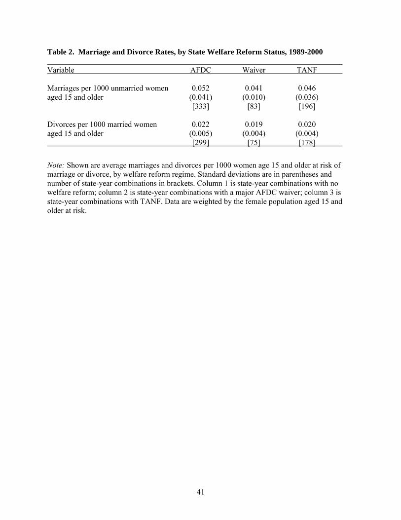
41

Table 2. Marriage and Divorce Rates, by State Welfare Reform Status, 1989-2000 Variable AFDC Waiver TANF

Marriages per 1000 unmarried women 0.052 0.041 0.046 aged 15 and older (0.041) (0.010) (0.036) [333] [83] [196] Divorces per 1000 married women 0.022 0.019 0.020 aged 15 and older (0.005) (0.004) (0.004) [299] [75] [178]

Note: Shown are average marriages and divorces per 1000 women age 15 and older at risk of marriage or divorce, by welfare reform regime. Standard deviations are in parentheses and number of state-year combinations in brackets. Column 1 is state-year combinations with no welfare reform; column 2 is state-year combinations with a major AFDC waiver; column 3 is state-year combinations with TANF. Data are weighted by the female population aged 15 and older at risk.

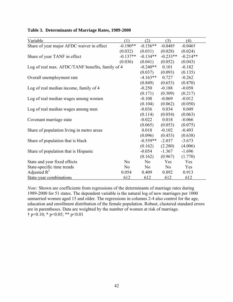
42

Table 3. Determinants of Marriage Rates, 1989-2000 Variable (1) (2) (3) (4) Share of year major AFDC waiver in effect -0.190** -0.156** -0.048† -0.046† (0.032) (0.031) (0.028) (0.024) Share of year TANF in effect -0.137** -0.134** -0.233** -0.214** (0.036) (0.041) (0.052) (0.043) Log of real max. AFDC/TANF benefits, family of 4 -0.240** 0.101 -0.182 (0.037) (0.093) (0.135) Overall unemployment rate -4.163** 0.727 -0.262 (0.849) (0.653) (0.870) Log of real median income, family of 4 -0.250 -0.188 -0.058 (0.171) (0.309) (0.217) Log of real median wages among women -0.108 -0.069 -0.012 (0.104) (0.062) (0.050) Log of real median wages among men -0.036 0.034 0.049 (0.114) (0.054) (0.063) Covenant marriage state -0.022 0.018 -0.066 (0.065) (0.053) (0.075) Share of population living in metro areas 0.018 -0.102 -0.493 (0.096) (0.453) (0.638) Share of population that is black -0.559** -2.037 -3.673 (0.162) (2.280) (4.006) Share of population that is Hispanic -0.054 -1.367 -1.696 (0.162) (0.967) (1.770) State and year fixed effects No No Yes Yes State-specific time trends No No No Yes Adjusted R2 0.054 0.409 0.892 0.913 State-year combinations 612 612 612 612 Note: Shown are coefficients from regressions of the determinants of marriage rates during 1989-2000 for 51 states. The dependent variable is the natural log of new marriages per 1000 unmarried women aged 15 and older. The regressions in columns 2-4 also control for the age, education and enrollment distribution of the female population. Robust, clustered standard errors are in parentheses. Data are weighted by the number of women at risk of marriage. † p<0.10; * p<0.05; ** p<0.01

43

Table 4. Determinants of Divorce Rates, 1989-2000 Variable (1) (2) (3) (4) Share of year major AFDC waiver in effect -0.118* -0.063* -0.055** -0.056** (0.042 (0.027) (0.018) (0.018) Share of year TANF in effect -0.075* 0.057† -0.126† -0.102 (0.030) (0.032) (0.065) (0.070) Log of real max. AFDC/TANF benefits, family of 4 -0.095* -0.033 -0.216† (0.042) (0.113) (0.125) Overall unemployment rate 0.247 -1.461* -1.772* (0.749) (0.676) (0.721) Log of real median income, family of 4 -0.983** -0.082 0.114 (0.152) (0.219) (0.180) Log of real median female weekly wages -0.141† -0.083† -0.025 (0.074) (0.044) (0.039) Log of real median male weekly wages 0.089 -0.075† -0.018 (0.071) (0.041) (0.044) Covenant marriage state 0.058 -0.055 -0.156* (0.057) (0.041) (0.070) Share of population living in metro areas 0.182* -0.232 -0.184 (0.074) (0.279) (0.324) Share of population that is black 0.377* -0.845 -6.669 (0.151) (1.662) (4.092) Share of population that is Hispanic -0.236 -5.163** -4.172* (0.164) (0.925) (1.912) State and year fixed effects No No Yes Yes State-specific time trends No No No Yes Adjusted R2 0.026 0.618 0.892 0.923 State-year combinations 552 552 552 552 Note: Shown are coefficients from regressions of the determinants of divorce rates during 1989-2000 for 46 states that report aggregate divorce data all years. The dependent variable is the natural log of new divorces per 1000 married women aged 15 and older. The regressions in columns 2-4 also control for the age, education and enrollment distribution of the female population. Robust, clustered standard errors are in parentheses. Data are weighted by the number of women at risk of divorce. † p<0.10; * p<0.05; ** p<0.01

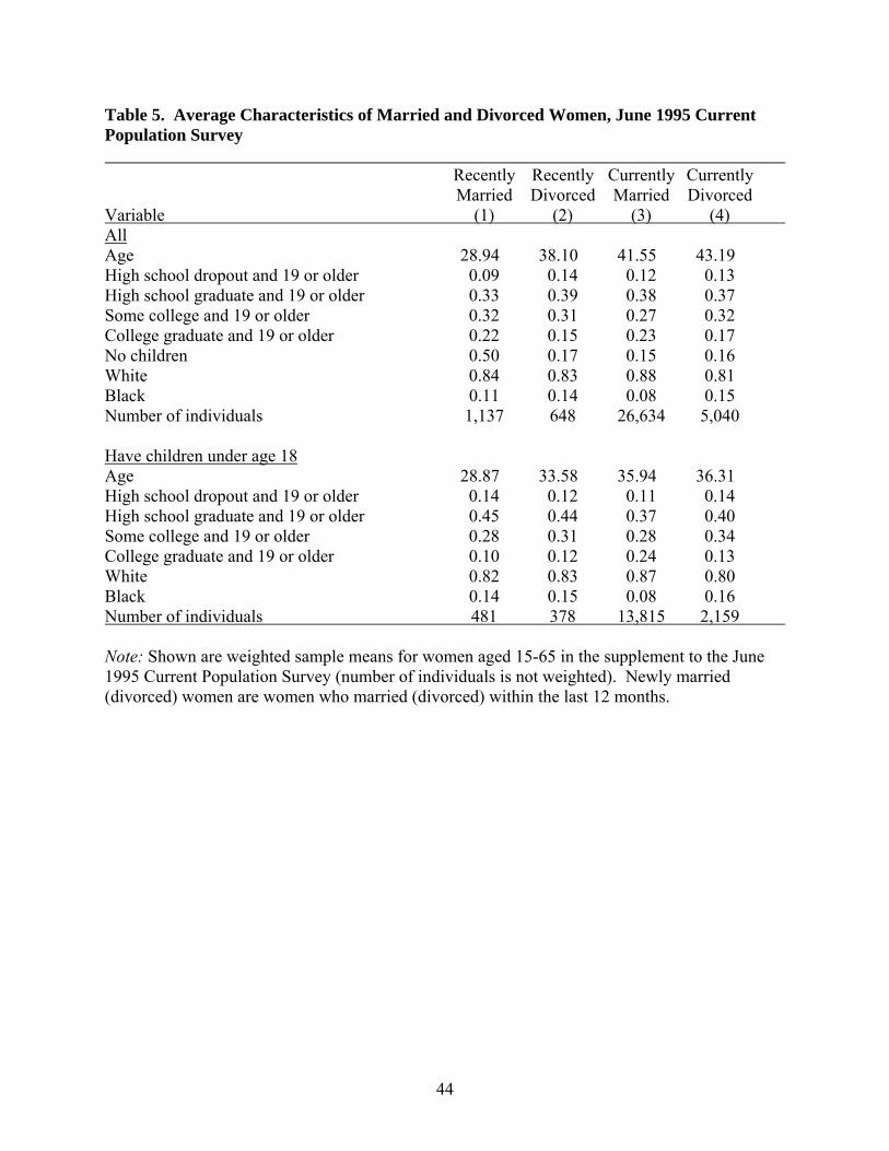
44

Table 5. Average Characteristics of Married and Divorced Women, June 1995 Current Population Survey Recently Recently Currently Currently Married Divorced Married Divorced Variable (1) (2) (3) (4) All Age 28.94 38.10 41.55 43.19 High school dropout and 19 or older 0.09 0.14 0.12 0.13 High school graduate and 19 or older 0.33 0.39 0.38 0.37 Some college and 19 or older 0.32 0.31 0.27 0.32 College graduate and 19 or older 0.22 0.15 0.23 0.17 No children 0.50 0.17 0.15 0.16 White 0.84 0.83 0.88 0.81 Black 0.11 0.14 0.08 0.15 Number of individuals 1,137 648 26,634 5,040 Have children under age 18 Age 28.87 33.58 35.94 36.31 High school dropout and 19 or older 0.14 0.12 0.11 0.14 High school graduate and 19 or older 0.45 0.44 0.37 0.40 Some college and 19 or older 0.28 0.31 0.28 0.34 College graduate and 19 or older 0.10 0.12 0.24 0.13 White 0.82 0.83 0.87 0.80 Black 0.14 0.15 0.08 0.16 Number of individuals 481 378 13,815 2,159 Note: Shown are weighted sample means for women aged 15-65 in the supplement to the June 1995 Current Population Survey (number of individuals is not weighted). Newly married (divorced) women are women who married (divorced) within the last 12 months.

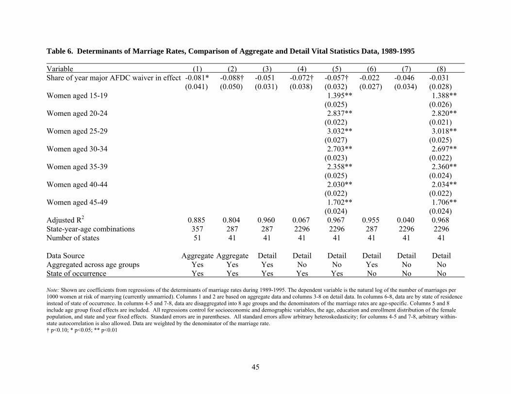
45

Table 6. Determinants of Marriage Rates, Comparison of Aggregate and Detail Vital Statistics Data, 1989-1995 Variable (1) (2) (3) (4) (5) (6) (7) (8) Share of year major AFDC waiver in effect -0.081* -0.088† -0.051 -0.072† -0.057† -0.022 -0.046 -0.031 (0.041) (0.050) (0.031) (0.038) (0.032) (0.027) (0.034) (0.028) Women aged 15-19 1.395** 1.388** (0.025) (0.026) Women aged 20-24 2.837** 2.820** (0.022) (0.021) Women aged 25-29 3.032** 3.018** (0.027) (0.025) Women aged 30-34 2.703** 2.697** (0.023) (0.022) Women aged 35-39 2.358** 2.360** (0.025) (0.024) Women aged 40-44 2.030** 2.034** (0.022) (0.022) Women aged 45-49 1.702** 1.706** (0.024) (0.024) Adjusted R2 0.885 0.804 0.960 0.067 0.967 0.955 0.040 0.968 State-year-age combinations 357 287 287 2296 2296 287 2296 2296 Number of states 51 41 41 41 41 41 41 41 Data Source Aggregate Aggregate Detail Detail Detail Detail Detail Detail Aggregated across age groups Yes Yes Yes No No Yes No No State of occurrence Yes Yes Yes Yes Yes No No No Note: Shown are coefficients from regressions of the determinants of marriage rates during 1989-1995. The dependent variable is the natural log of the number of marriages per 1000 women at risk of marrying (currently unmarried). Columns 1 and 2 are based on aggregate data and columns 3-8 on detail data. In columns 6-8, data are by state of residence instead of state of occurrence. In columns 4-5 and 7-8, data are disaggregated into 8 age groups and the denominators of the marriage rates are age-specific. Columns 5 and 8 include age group fixed effects are included. All regressions control for socioeconomic and demographic variables, the age, education and enrollment distribution of the female population, and state and year fixed effects. Standard errors are in parentheses. All standard errors allow arbitrary heteroskedasticity; for columns 4-5 and 7-8, arbitrary within-state autocorrelation is also allowed. Data are weighted by the denominator of the marriage rate. † p<0.10; * p<0.05; ** p<0.01

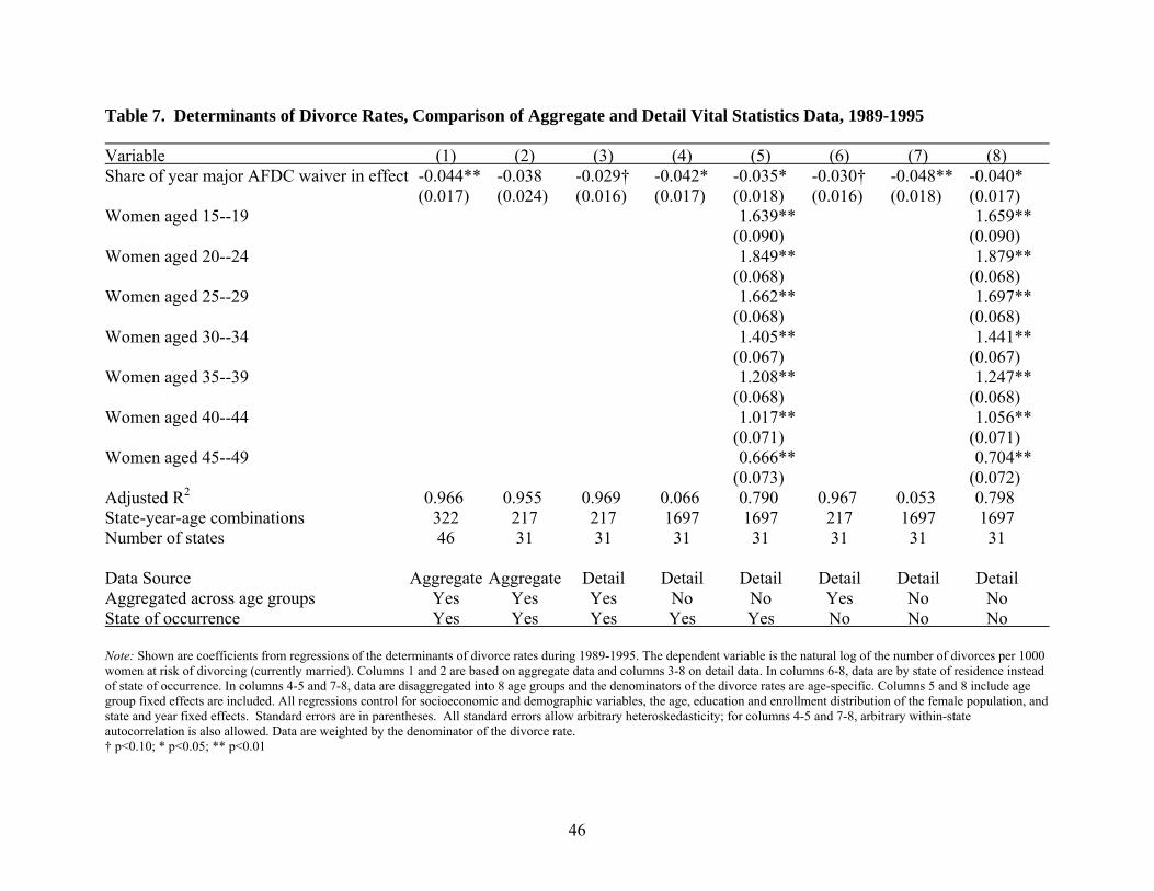
46

Table 7. Determinants of Divorce Rates, Comparison of Aggregate and Detail Vital Statistics Data, 1989-1995 Variable (1) (2) (3) (4) (5) (6) (7) (8) Share of year major AFDC waiver in effect -0.044** -0.038 -0.029† -0.042* -0.035* -0.030† -0.048** -0.040* (0.017) (0.024) (0.016) (0.017) (0.018) (0.016) (0.018) (0.017) Women aged 15--19 1.639** 1.659** (0.090) (0.090) Women aged 20--24 1.849** 1.879** (0.068) (0.068) Women aged 25--29 1.662** 1.697** (0.068) (0.068) Women aged 30--34 1.405** 1.441** (0.067) (0.067) Women aged 35--39 1.208** 1.247** (0.068) (0.068) Women aged 40--44 1.017** 1.056** (0.071) (0.071) Women aged 45--49 0.666** 0.704** (0.073) (0.072) Adjusted R2 0.966 0.955 0.969 0.066 0.790 0.967 0.053 0.798 State-year-age combinations 322 217 217 1697 1697 217 1697 1697 Number of states 46 31 31 31 31 31 31 31 Data Source Aggregate Aggregate Detail Detail Detail Detail Detail Detail Aggregated across age groups Yes Yes Yes No No Yes No No State of occurrence Yes Yes Yes Yes Yes No No No Note: Shown are coefficients from regressions of the determinants of divorce rates during 1989-1995. The dependent variable is the natural log of the number of divorces per 1000 women at risk of divorcing (currently married). Columns 1 and 2 are based on aggregate data and columns 3-8 on detail data. In columns 6-8, data are by state of residence instead of state of occurrence. In columns 4-5 and 7-8, data are disaggregated into 8 age groups and the denominators of the divorce rates are age-specific. Columns 5 and 8 include age group fixed effects are included. All regressions control for socioeconomic and demographic variables, the age, education and enrollment distribution of the female population, and state and year fixed effects. Standard errors are in parentheses. All standard errors allow arbitrary heteroskedasticity; for columns 4-5 and 7-8, arbitrary within-state autocorrelation is also allowed. Data are weighted by the denominator of the divorce rate. † p<0.10; * p<0.05; ** p<0.01