The Impact of Transaction Tax on Stock Markets:

Evidence from an emerging market

Li ZhangDepartment of EconomicsEast Carolina University

M.S. Research Paper

Under the guidance ofDr. Dong Li

Abstract

This paper provides empirical study on the behavior of the Shanghai and the Shenzhen stock

exchanges after the Chinese government announced to increase the securities transaction tax from

0.3% to 0.5% in May 9th, 1997. We examine the impact of the increased transaction tax on the

volatility of stock returns and tax revenue. We find that the return volatility significantly

increased. We also find that because the volume decreased considerably, the increase in the tax

revenue is relatively small compared to the increased level of the tax rate.

1

1.Introduction

There are quite divergent opinions on the effect of increasing the securities

transaction tax on the stock markets. Proponents of the securities transaction tax have

suggested that the tax is an instrument to reduce stock market volatility, raise tax revenue,

direct the investors and managers to behave in the long-run prospective, improve market

efficiency, and fairly reallocate the social wealth. But opponents have argued against it

by both theory and empirical study. Schwert and Seguin (1993) reviewed those opinions

with respect to the costs, benefits and unresolved questions on the transaction tax. We can

find that whether the benefit of the transaction tax could outweigh its cost is still a hot

polemic unsettled. The main controversies are presented as follows:

1) Reduce excess stock return volatility or not

Proponents believe that the securities transaction tax could act as a fundamental

function to reduce excess stock return volatility. They argue that considerable price

volatility in stock markets is from the activities of “noise traders”. Noise traders do not

analyze the intrinsic value of stocks when they submit orders, and such behavior causes

securities prices to diverge significantly from their fundamental values. Such behaviors

are harmful to the economy. So the government should exert pressure to reduce noise

traders’ activities. Proponents argue that increasing the transaction tax is a great tool to

achieve the goal. When the transaction tax is increased, the transaction costs are

increased. Noise traders would be “punished” for each of their short-term speculative

2

activities. As their processing of speculative transactions turns out to meet resistance, the

noise traders are encouraged to spend more time on studying the intrinsic value of the

securities. Therefore, many speculative transactions would be replaced, and the influence

of noise traders on the stock market would be reduced. Therefore, the short-term

speculative trading volume, which is the source of excess volatility, would be diminished.

This outcome will in turn benefit fundamental investors. Thus, many proponents hold the

opinion that tax functions as a strong weapon against excessive speculation. One of

Tobin’s (1984) analyses best concluded this mechanism: “throw sand in the gears”. The

gears are looked at as our excessively well-functioning financial markets, and sand is the

transaction tax. The “sand” limits activities of speculators. The financial market will be

more balanced and stable.

However, there are also many opponents to show their doubts on such arguments.

They believe that decreasing volatility would not surely happen as a consequence of

increasing the transaction tax. This point is based on the fact that the transaction tax treats

each trader indifferently. The transaction tax would influence not only the noise traders,

but also those informed traders who play the role of decreasing volatility in the stock

market. Only when the tax has a greater limiting effect on the activities of noise traders

than on price-stabilizers and informed traders, we can say that the transaction tax could

play a role in decreasing the volatility. The estimate of its effect on volatility is not

reliable until all traders in the stock market are taken into consideration. We cannot

exclude the possibility that the transaction tax could increase volatility by affecting

rational traders more seriously than noise traders. Besides the theoretical analyses,

3

researchers have also done some empirical tests on the effect of increasing transaction tax

on price volatility. One example is Umlauf’s (1993) study on Swedish stock market

during 1980-1987. Umlauf found that, contrary to what some proponents expected, after

imposing the transaction tax, daily variances were highest during the greatest tax regime

(the tax rate was 2% from July 1986 to Dec 1987). Jones and Seguin (1997) examined the

effect of commission deregulation in the United States during 1975, which reduces

transaction costs, on price volatility. Their empirical results showed that the deregulation

of fixed commissions increases volume, and “the effect of this volume increase was to

reduce volatility of returns.” So, opponents believe that the securities transaction tax

would not decrease volatility.

2) Increase tax revenues or not

One of the fundamental motivations for increasing the transaction tax is to

increase tax revenues. Proponents believe that as the tax rate increases, the tax revenue

would increase significantly. Although this apparently seems so, opponents have strong

doubts about it after more careful examination. They argue that in theory, tax revenue is

the product of three parameters, tax rate, volume weighted average price level, and the

quantity of transactions. By increasing the trading cost, one of the factors, tax rate, would

increase, but at the same time, the other two factors, the quantity of transactions, as well

as the price level, could considerably decrease. As the traders’ profit is greatly affected

by the increased cost of transaction tax, the traders will try to diminish their “loss” in

paying taxes. One of their consequent actions is to reduce their transactions, which would

4

directly decrease the quantity of transactions in the stock market. Another profitable

action for traders is to shift their trades from securities of short-term nature to longer-

maturity securities because the short-term securities are traded more frequently and thus

have a higher tax burden. A more serious problem is for traders to migrate their

investment from their home country to foreign exchanges in order to seek lower

transaction tax and keep their profit. The stock market of their home country is therefore

shrinking by losing transaction volume. Umlauf (1993) found that in the Swedish stock

market, “when the 2% tax was introduced in 1986, 60% of the trading volume of the 11

most actively traded Swedish share classes migrated to London to avoid taxes.” By using

the Swedish and British systems to examine its international experience, Campbell and

Froot (1993) pointed out that these three effects on trading volume “… can be important.

Estimated revenues from increasing transaction tax will be correspondingly overstated if

they ignore such behavioral effects.” One empirical study to test the effects is to analyze

the elasticity of trading volume with respect to trading cost. Schwert and Seguin (1993)

pointed out that “based on the limited evidence available to date, it seems that the

elasticity of trading volume with respect to transaction costs is between –0.25 and –1.35.”

So as the tax rate increases, the trading volume would decrease. Secondly, many

researchers believe that the transaction tax would also reduce the prices of securities to

reduce the tax revenue. As the transaction cost increases, the required rates of return

would increase. And as the required rates of return increase, the prices of securities would

be reduced. So, with the declining effect on the tax revenue by the decreased transaction

volume and decreased transaction prices, it is unclear whether the transaction tax revenue

would increase. In addition to the direct effect on transaction tax revenue, Umlauf (1993)

5

argued that there would be a secondary effect of introducing a transaction tax on capital

gains tax revenue. He pointed out that “the capital gains tax revenue fell so much in

response to lower levels of trading that transaction tax revenues were entirely offset.” So,

both transaction tax revenue and capital gains tax revenue would be considerably affected

by increasing the transaction tax rate.

3) Effects on capital market efficiency

Another controversial issue is whether the transaction tax would improve the

efficiency in allocating resources in the capital market. Proponents believe that it could

make both managers and traders have long-term horizons rather than short-term horizons.

Sometimes managers’ myopic allocation or traders’ myopic investment on short-run

projects may be harmful to long-run projects and constrain the development of both

companies and the economy. The securities transaction tax may discourage such

unproductive activities because these activities are heavily taxed and thus unprofitable.

Lengthening the horizons of corporate managers would help allocate resources more

efficiently. Opponents concede that the transaction tax may improve capital market

efficiency in some respects, but they believe that its negative effects on the efficiency of

the capital markets are considerable too. One of its negative effects is the distortion of

optimal portfolios. They argue that the optimal portfolio would be most efficient when

there are no tax burdens on securities. When taxes are added to the securities, the relative

cost of different classes of securities would change, because the transaction tax has

different effects on them. For example, those securities with short-term nature that are

6

traded frequently would be affected most negatively by increasing the transaction tax.

When relative transaction costs of various stocks’ change, the optimal portfolio would

change accordingly, distorting the allocation resources from the original portfolio and

making a less efficient capital market. Another inefficiency caused by the transaction tax

would be an indirect effect on the liquidity of financial assets. As the transaction cost

increases, the frequency of transactions would be decreased to avoid a higher tax burden.

When it happens that an asset’s price is currently misleading and is inconsistent with its

intrinsic value, it would take longer to correct for the discrepancy because of the lack of

enough transactions. In these cases, the capital market becomes inefficient.

4) Fairly reallocate the social wealth or not

Proponents also believe that the securities transaction tax would help government

reallocate the wealth in the society fairly. They argue that the wealthy have more

financial assets and tend to trade them more frequently. So the wealthy would have to

suffer more from the increased tax. A bigger proportion of the profits would be extracted

from the wealthy for their frequent speculation and trading. Government collects these

taxes and reallocates them to the non-wealthy by government spending. Thus, the

transaction tax would alleviate the tension of the concentration of the social wealth in

some particular groups. However, opponents find that this is not so optimistic as it seems.

Instead, the transaction tax would hurt the whole population in the society. One fact is

that the number of stockowners is huge, and not just the wealthy are direct owners. So,

the increased transaction tax also hurts the non-wealthy each time they trade. Another

7

fact is that all the stockowners suffer capital loss. The cost of transaction will directly

reduce the asset value, as we have mentioned above, and cause the current owners to lose

their wealth immediately. In the end, it is still uncertain whether the securities transaction

tax could transfer part of the wealth from the wealthy to the non-wealthy or not.

After the market closed on May 9th, 1997 (Friday), the Chinese government

announced the securities transaction tax to change from 0.3% to 0.5% immediately. In

this paper, following Umlauf’s (1993) empirical study on the Swedish stock exchanges,

and Jones and Seguin’s (1997) study on the United States stock exchanges, I provide

additional study on the Chinese stock exchanges and add empirical evidence to current

discussions on the securities transaction tax. Section 2 discusses the data. Section 3

presents the methodology and results, and section 4 concludes the paper.

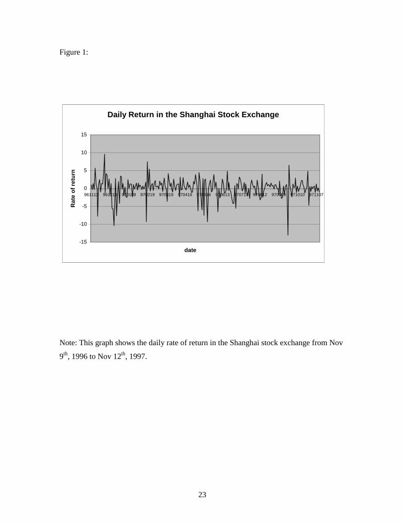
2.Data

The data in this paper is from DataStream. The data includes the value-weighted

average indexes, and shares of trading stocks for the Shanghai A stocks and the Shenzhen

A stocks. The data spans from Nov 9th, 1996 to Nov 12th, 1997, excluding holidays when

there were no transactions. In this paper, the rate of return is defined as

)log(*100 1−= ttt IndexIndexr , and the volume is defined as (trading volume)/

1,000,000. Figure 1 and figure 2 show the daily rate of return in the Shanghai and the

Shenzhen stock exchanges during our sample.

8

Now I provide a brief description of the Chinese stock market. There are two

nationwide equity markets in China: the Shanghai stock exchange and the Shenzhen

stock exchange. They are under the supervision of the China Securities Regulatory

Commission. The transactions follow the rules of price priority and time priority. There

are several kinds of stocks in China. Two major kinds are A stocks and B stocks. Their

fundamental difference is that A stocks should traded by the Chinese domestic citizens

with Chinese currency Renminbi (RMB: Chinese monetary unit) 1, while B stocks should

be traded by foreign investors with foreign monetary unit. Despite their differences, in

many respects, A stocks and B stocks follow the same rules. For example, except for the

first exchange day, the percentage of change is limited to 10% per day. There are five

major industrial sectors: Industry, Commerce, Real estate, Utility, and comprehensive.

The Shanghai stock exchange was established on Nov 26th, 1990. At the end of

1996, there were 293 listed companies. There were 287 A stocks listed companies, and

42 B stocks listed companies. The total market value was RMB 547.78 billion, and the

outstanding market value was RMB 140.87 billion. The total shares of stocks were 57.08

billion. The Shenzhen stock exchange was established on Dec 1st, 1990. At the end of

1996, there were 237 listed companies. The total market value was RMB 436.4 billion,

and the outstanding market value was RMB 45.8 billion. The total shares of stocks were

43.95 billion.

1 The exchange rate was quite stable around $1 = RMB 8.29 through the sample period in this paper.

9

On May 9th, 1997, the tax rate was announced to increase from 0.3% to 0.5%. The

central government conserved 88% of the securities transaction tax revenue, and the local

government conserved 12% of them. Besides the transaction tax, the investors were

charged a commission fee for each trade2.

3.Methodology and Results

3.1.Analysis of Volatility

To examine the transaction tax effect on market volatility, we test the equity of

variances before and after the announcement. Before using techniques and calculating

test statistics, we should test for normality first, because some statistics in this paper are

sensitive to normality assumption. For example, to test the significance level for Levene

test statistics, we cannot check them with common F-table if the population is not

normally distributed. In this case, we should use bootstrapping technique, which is robust

under non-normality. So, we must first examine the normality.

3.1.1Test for normality

The samples used in this paper are defined as follows: May 9th, 1997 was defined

as –1 event day, because the announcement was made after market closed on that day,

and such announcement had no effect on that day’s trading. May 12th, 1997, which was

2 The commission was regulated by not to exceed RMB 4.0 (which is approximately US$ 0.48).

10

Monday, was defined as +1 day, because it was the first day after the announcement. May

8th was –2 day, and May 13th was +2 day, and so on.

I use samples of +/-15 days, +/-30 days, +/-45 days, +/-60 days, and +/-75 days

around the announcement respectively to test for normality of return.

Table 1 and table 2 show the results for the Shanghai and the Shenzhen stock

exchanges. For the Shanghai stock exchange, the signs for skewness are all negative,

which indicates that the distribution for rate of return skewed left, and all the signs for

kurtosis are positive, which indicates that the distribution are heavy tailed. Examining the

significance levels, we should use the Shapiro-Wilk test because the sample size is less

than 20003. I find that all the p values in all the samples are smaller than 1%, so we can

reject the null hypothesis that the distributions are normal at 1% significance level. We

find similar results for the Shenzhen stock exchange, skewed left, and heavy tailed, and

not normally distributed. Using another method, the Jarque-Bera test, which jointly tests

the skewness and kurtosis, I get the same results. All the p values are less than 1% in all

the samples in both the Shanghai and the Shenzhen stock exchanges. So, I can reject the

null hypothesis of normal distribution at 1% significance level.

3 Note: If the sample size is less than 2, 000, the Shapiro-Wilk statistic W is computed to test normality. Wis the ratio of the best estimator of the variance to the usual corrected sum of squares estimator of thevariance.

11

3.1.2 Levene test statistic

Our null hypothesis for testing volatility is: H0:22

21 σσ = , and H1:

22

21 σσ ≠ , where

21σ is the variance before the announcement, and 2

2σ is the variance after the

announcement. Levene (1960) proposed a statistic for a test of the equality of variance.

We use the Levene test statistics to test the null hypothesis.

Let ijx be the j th ( ),..., inij = observation in the i th group ( ),...,,1 gi = where g is

the number of groups in the sample (in our model, g =2), and let || iijij xxz −= , where ix

is the sample mean for each group. The Levene test statistic is defined as:

∑∑ ∑∑

−−

−−=

i ii j iij

i ii

nzz

gzznW

)1(.)(

)1(..).(2

2

0

where

iiji nzz ∑= and ∑∑∑= iij nzz..

Levene test is the ratio of between group variation and within group variation.

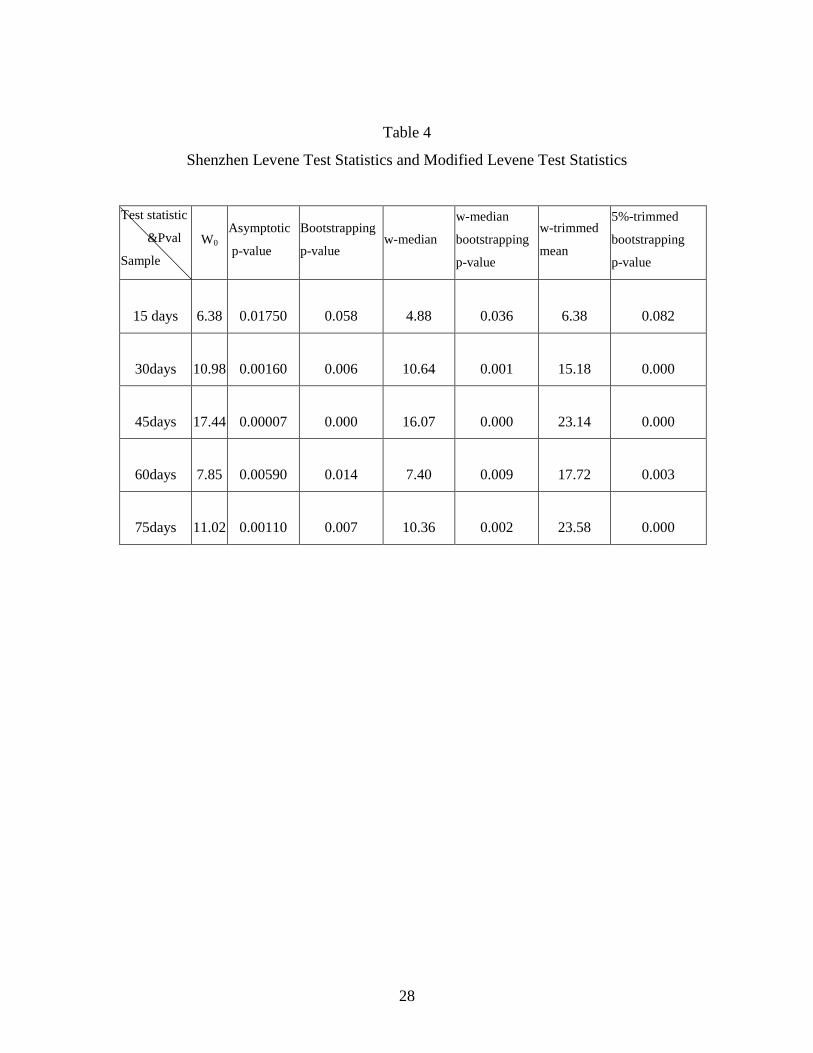
Table 3 and table 4 show the results of the Levene test statistics in the Shanghai and the

Shenzhen stock exchanges. Brown and Forsythe (1974) pointed out that the common F-

test could check the significance levels of Levene test statistics if the underlying

population is distributed Gaussian. The critical values of 0W are obtained from the F-

12

table with g – 1 and ∑ −i in )1( degree of freedom. So I get the asymptotic p-values,

which are shown in table 3 and table 4.

In the Shanghai stock exchange, we can reject the null hypothesis at 1%

significance level for the +/-45 days samples, at 5% confidence level for the +/-30 days

and +/- 75 days samples, at 10% level for the +/-15 days sample. We don’t reject the null

at 10% level for the +/- 60 days sample. In the Shenzhen stock exchange, we can reject

the null hypothesis that the volatility does not change after the announcement at 1%

confident level for the samples of the +/-30 days, +/-45 days, +/-60 days, and +/-75 days.

We can reject the null hypothesis at 5% level for the +/-15 days sample.

But the result above would be misleading when the assumption of normality were

violated. I will resort to the bootstrapping method to deal with this complication.

3.1.3. Bootstrapping for Levene test statistic

First, I draw 2 k daily returns randomly from our samples, and divide the random

sample into two groups: k days before the announcement and k days after the

announcement. And we calculate the Levene test statistic W . Then we repeated such

procedure m times. In this way, we get a series of Levene test statistics: mWWW ,..., 21 .

Secondly, we calculate the bootstrapping P value for 0W . The significance level of 0W is

known as the percentiles in the distribution of the bootstrapping series we get in the first

step. Let’s suppose it ranks U in the sample. The p value is Prob { )(xN > 0W } (where the

13

)(xN is the bootstrapping series), and it is equal to 1- mU / . Further, in order to avoid

arbitraries of sample size, we let k = 15, 30, 45, 60, 75. See Efron and Tibshirani (1993)

for detailed bootstrap techniques.

Table 3 shows the bootstrapping p values in the Shanghai stock exchange. The

variances are significantly different at 5% significant level for the samples of +/-45 days

and +/-75 days, and at 10% level for the +/- 30 days sample. Table 4 shows the

bootstrapping p values in the Shenzhen stock exchange. The variances are significantly

different at 1% significant level for the samples of +/-30 days, +/-45 days, and +/-75

days, and at 5% level for the +/-60 days sample, and at 10% level for the +/-15 days

sample.

3.1.4 Modified Levene test statistic: median adjusted Levene and 5% - trimmed Levene

There are more robust estimators than the original Levene test statistic when the

underlying population is skew. These estimators are to use median, or 5% - trimmed

mean (the choice of percent of trimming is arbitrary), in place of the mean to calculate

Levene statistic. The 5% - trimmed mean is the mean after deleting the largest 5%

observations and the smallest 5% observations in that group. Considering our samples are

skew, we resort to these modified Levene estimators.

Table 3 shows the modified Levene test statistics and their bootstrapping P values

in each sample in the Shanghai stock exchange, and Table 4 shows the results in the

14

Shenzhen stock exchange. In the Shanghai stock exchange, using the median-adjusted

Levene test, the variances are significantly different at 1% significance level for the +/-45

days sample, at 5% level for the +/-30 days sample, and at 10% level for the +/-75 days

sample. Using the 5%-trimmed Levene test, the variances are significantly different at

1% significance for the +/-45 days and +/-75 days samples, and at 5% level for the +/-30

days and +/-60 days samples, but they are not significantly different for the +/-15 days

sample. So by using the 5%-trimmed mean Levene test, the null hypothesis could be

rejected at 5% significance in four out of five samples.

In the Shenzhen stock exchange, using the median-adjusted Levene test, I find

that for the +/-15 days sample, the variances are significantly different at 5% significance

level. For all the other samples, the variances are significantly different at 1%

significance level. Using the 5%- trimmed Levene test, the variances are significantly

different at 1% level for the samples of +/-30 days, +/-45 days, +/-60 days, and +/-75

days. For the +/-15 days sample, we can reject the null hypothesis at 10% significance

level.

By using the original Levene test and the modified Levene test, we find that the

volatility changed significantly. By examining Table 5 and Table 6, we can see that the

market volatility increased with the tax rate, contrary to the scenario described by the

proponents of the stock transaction tax.

15

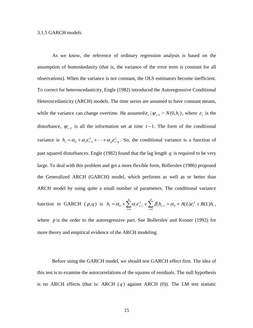
3.1.5 GARCH models

As we know, the reference of ordinary regression analysis is based on the

assumption of homoskedasity (that is, the variance of the error term is constant for all

observations). When the variance is not constant, the OLS estimators become inefficient.

To correct for heteroscedasticity, Engle (1982) introduced the Autoregressive Conditional

Heteroscedasticity (ARCH) models. The time series are assumed to have constant means,

while the variance can change overtime. He assumed ),0(~| 1 ttt hN−ψε , where tε is the

disturbance, 1−tψ is all the information set at time 1−t . The form of the conditional

variance is 22110 qtqtth −− +++= εαεαα L . So, the conditional variance is a function of

past squared disturbances. Engle (1982) found that the lag length q is required to be very

large. To deal with this problem and get a more flexible form, Bollerslev (1986) proposed

the Generalized ARCH (GARCH) model, which performs as well as or better than

ARCH model by using quite a small number of parameters. The conditional variance

function in GARCH ( qp, ) is tt

p

iiti

q

iitit hLBLAhh )()( 2

011

20 ++=++= ∑∑

=−

=− εαβεαα ,

where p is the order to the autoregressive part. See Bollerslev and Kroner (1992) for

more theory and empirical evidence of the ARCH modeling.

Before using the GARCH model, we should test GARCH effect first. The idea of

this test is to examine the autocorrelations of the squares of residuals. The null hypothesis

is no ARCH effects (that is: ARCH ( q ) against ARCH (0)). The LM test statistic

16

is 22 TR=χ , where 2R is from the regression of 2tl on a constant and q lagged values. The

test statistic follows a limiting chi-squared distribution with q degrees of freedom. If it is

greater than the critical value, we can reject the null hypothesis. Bollerslev (1986)

suggested a Lagrange multiplier statistic, which is even easier to compute. I use

ARCHTEST option to test the absence of ARCH effects. I find that in our sample of +/-6

months, all the p > LM values of the twelve lags in the Shenzhen stock exchange are

smaller than 0.01, and in the Shanghai stock exchange, the p values of the first five lags

are smaller than 0.05. So, we can reject the null hypothesis that there are no ARCH

effects. We should use GARCH models to examine the volatility.

We estimate the GARCH models using the maximum likelihood estimators’

method. It maximizes the following function based on the assumption of normal

distribution. The log-likelihood function is:

++−=∑

=2

22

1

ln)2ln(2

1ln

t

tt

T

t

Lσεσπ .

I defined a dummy variable After, which equals 1 when the observation is after

the announcement, and equals 0 otherwise. In the GARCH (1,1) model, I add the Volume

and After in both the mean function and the variance function. The result in the Shanghai

stock exchange is:

17

)33.7(

)11.0(

82.0

)86.3()81.3(

)52.0()07.0(

02.225.0

)00.0()1994119(

)155.6()153.5(

)2069.1(81

)72.0(

)38.0(

27.0

)50.1()56.0(

)06.0()42.0(

10.023.0

211

=+

==++

−==−−−

−−=

+−=

−=−=

+−

=

−−

t

Volume

tt

After

tt

EE

hEE

h

t

After

tt

Volume

r

tt

t

tt

ε

ε

In the mean function, the coefficient on “after” indicates the effect of raising the

transaction tax on the mean of rate of return. “Volume” can be considered as a proxy for

arrived information in the market. [See Hiemstra and Jones (1994)]

In the mean function in the Shanghai stock exchange, the coefficient on After is

negative, but it is not significant. The coefficient on Volume is positive. In the variance

function, the coefficient on After is positive and significant at 1% significance level. The

coefficient on Volume is positive and significant at 1% level. It indicates that the variance

of rate of return increases as the volume increases.

The result in the Shenzhen stock exchange is:

)94.0(

)20.0(

18.0

)62.0()84.2(

)74.0()10.0(

46.030.0

)13.3()64.0(

)15.0()29.1(

46.082.0

)15.0(

)57.0(

08.0

)15.1()53.0(

)11.0()98.0(

13.051.0

211

=+

==++

==−=

+−=

−=−=

+−

=

−−

t

volume

tt

After

tt

h

h

t

After

tt

volume

r

tt

t

tt

ε

ε

18

In the mean function, the coefficient on After is negative but insignificant. The

coefficient on Volume is positive but insignificant. In the variance function, the

coefficients on After and Volume are both positive, but neither of them is significant.

I find that the results of GARCH models in the Shanghai stock exchange support

that the volatility increased after the announcement, but those in the Shenzhen stock

exchange do not sufficiently support it.

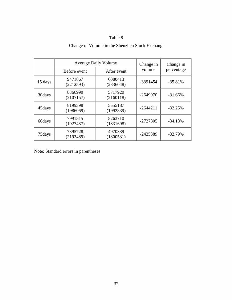
3.2.Analysis of tax revenue by examining trading volume;

Table 7 and table 8 show the trading volumes in 15, 30, 45, 60, and 75 days

before and after the announcement and their changes in the Shanghai and Shenzhen stock

exchanges respectively. We find that they decrease considerably. In the Shanghai stock

exchange, we find that the volume in the +/-60 days sample decreases 43.86%, and in the

+/- 45 days sample, it decreases 43.62%. The effect on the trading volume in the

Shenzhen stock exchange is considerable too. In the +/-15 days sample, it decreases

35.81%, and in the +/-60 days sample, it decreases 34.13%, and so on.

Assuming the stock price constant and using the volume change percentage as

that in the +/-75 days sample, I calculate the effect of increasing the securities transaction

tax on tax revenue in the Shanghai and the Shenzhen stock exchanges. In Shanghai, the

volume decreases 38.47%, and in the Shenzhen stock exchange, it decreases 32.79%. The

tax rate in both stock exchanges increases 66.67%. So, the result is that the tax revenue

19

increases 0.26% in Shanghai and increases 12.02% in the Shenzhen stock exchange after

the announcement of raising the transaction tax rate. Comparing the change level of tax

revenue to the increased level of the tax rate, I find that the increased level of tax revenue

is much smaller because the volume decreases considerably after raising the tax rate, and

it significantly offsets the benefit on tax revenue.

The elasticity of trading volume with respect to tax rate is the percentage change

in volume when the tax rate changes 1%. The elasticity in the Shanghai stock exchange is

–0.58 and is –0.49 in the Shenzhen stock exchange. The elasticity of tax revenue with

respect to tax rate is the percentage change in tax revenue when the tax rate changes 1%.

The elasticity in the Shanghai stock exchange is 0.004 and is 0.18 in the Shenzhen stock

exchange. However, I do not measure other factors that could affect the elasticity, such

as commission and other transaction costs, so my estimate on the elasticity is limited to

these assumptions. As summarized by Schwert and Seguin (1993), the elasticity of

trading volume with respect to the transaction cost lies between –0.25 and –1.35. Our

results are consistent with previous studies.

4.Conclusion

In this paper, by examining the Chinese stock markets, I add one observation to

the literature on the impact of transaction cost (tax) on the stock markets.

20

For the relationship between the securities transaction tax and the stock return

volatility, I conclude that the volatility increases significantly in both the Shanghai and

the Shenzhen stock exchanges after increasing the transaction tax. It is contrary to many

experts and government officials’ speculation before the event. The theory that the

increased transaction tax would reduce market volatility is not supported by our empirical

evidence.

On the tax revenue, I conclude that the tax revenue did not increase as much as

the proponents of the tax expected. Investors reacted to the increased tax dramatically.

The decrease in trading volume significantly offsets the increased tax rate. Thus, the tax

revenue didn’t increase much.

21

Reference

Bollerslev, T. (1986) Generalized autoregressive conditional heteroscedasticity, Journal

of Econometrics, 31, 307-327

Bollerslev, T., Chou, R.Y. and Kroner, K.F. (1992) ARCH modeling in finance: a review

of the theory and empirical evidence, Journal of Econometrics, 52, 5-59

Campbell, J.Y; Froot, K.A. (1993) International Experiences with Securities Transaction

Taxes, National Bureau of Economic Research Working Paper: 4587, December 1993, 28

pp.

Hiemstra.C Jones and J.D. (1994) Testing for Linear and Nonlinear Granger Causality in

the Stock Price-Volume Relation in Journal of Finance, vol. 49, no. 5, December 1994,

1639-1664

Efron, B; Tibshirani, R.J. (1993) An Introduction to the Bootstrap, London: Chapman &

Hall

Engle, R.F. (1982) Autoregressive conditional heteroscedasticity with estimates of the

variance of U.K. Inflation, Econometrica, 50, 987-1008

Jones, C. and Seguin, P.J, (1997) Transaction costs and price volatility: Evidence from

commission deregulation, American Economic Review, 84, 728-737

Levene, H. (1960) Robust tests for equality of variances, in I.Olkin, ed., Contributions toProbability and Statistics, Palo Alto, Calif.: Stanford University Press, 278-92

Brown, M.B. and Forsythe, A.B. (1974) Robust Tests for the Equality of Variances,

Journal of the American Statistical Association, vol. 69, June, 1974, pp. 364-367

22

Schwert, G.W. and Seguin, P.J. (1993) Securities transaction taxes: an overview of costs,

benefits and unsolved questions, Financial Analysts Journal, 49, 27-35

Tobin, J. (1984) On the efficiency of the financial system, Lloyds Bank Review 153, 1-15

Umlauf, S.R. (1993) Transaction taxes and the behavior of the Swedish stock market,

Journal of Financial Economics, 33, 227-240

23

Figure 1:

Daily Return in the Shanghai Stock Exchange

-15

-10

-5

0

5

10

15

961112 961210 970108 970219 970319 970416 970516 970613 970715 970812 970909 971010 971107

date

Rat

eo

fre

turn

Note: This graph shows the daily rate of return in the Shanghai stock exchange from Nov

9th, 1996 to Nov 12th, 1997.

24

Figure 2:

Note: This graph shows the daily rate of return in the Shenzhen stock exchange from Nov

9th, 1996 to Nov 12th, 1997.

Daily Return in the Shenzhen Stock Exchange

-12

-10

-8

-6

-4

-2

0

2

4

6

8

961112 961210 970108 970219 970319 970416 970516 970613 970715 970812 970909 971010 971107

date

rate

of

retu

rn

25

Table 1

Test for Normality in the Shanghai Stock Exchange

Mean(StandardDeviation)

Skewness KurtosisShapiro-Wilk

statistic test P <W

+/-15 days-0.122(3.31)

-1.38 1.54 0.0012

+/-30 days0.097(2.80)

-1.31 2.38 0.0001

+/-45 days0.125(2.63)

-1.23 2.13 <0.0001

+/-60days0.184(2.64)

-1.13 3.02 <0.0001

+/-75 days0.189(2.46)

-1.13 3.41 <0.0001

26

Table 2

Test for Normality in the Shenzhen Stock Exchange

Mean(StandardDeviation)

Skewness KurtosisShapiro-Wilk

statistic test P <W

+/-15 days-0.128(3.77)

-1.39 1.63 0.0008

+/-30 days-0.007(3.25)

-1.09 2.00 0.0009

+/-45 days0.06

(3.05)-1.19 2.21 <0.0001

+/-60days0.09

(2.97)-1.28 2.87 <0.0001

+/-75 days0.11

(2.76)-1.31 3.29 <0.0001

27

Table 3

Shanghai Levene Test Statistics and Modified Levene Test Statistics

Test statistic

& pval

Sample

W0

Asymptotic

p-value

Bootstrapping

p-valuew-median

w-median

bootstrapping

p-value

5%-trimmed

mean

5%-trimmed

bootstrapping

p-value

15days 3.31 0.0797 0.144 2.51 0.133 3.31 0.201

30days 4.69 0.0345 0.059 4.10 0.043 6.87 0.024

45days 7.29 0.0083 0.011 6.42 0.008 11.27 0.009

60days 2.19 0.1418 0.184 1.85 0.159 8.68 0.042

75days 4.54 0.0347 0.044 3.96 0.057 14.56 0.004

28

Table 4

Shenzhen Levene Test Statistics and Modified Levene Test Statistics

Test statistic

&Pval

Sample

W0

Asymptotic

p-value

Bootstrapping

p-valuew-median

w-median

bootstrapping

p-value

w-trimmed

mean

5%-trimmed

bootstrapping

p-value

15 days 6.38 0.01750 0.058 4.88 0.036 6.38 0.082

30days 10.98 0.00160 0.006 10.64 0.001 15.18 0.000

45days 17.44 0.00007 0.000 16.07 0.000 23.14 0.000

60days 7.85 0.00590 0.014 7.40 0.009 17.72 0.003

75days 11.02 0.00110 0.007 10.36 0.002 23.58 0.000

29

Table 5

Descriptive Statistics Before and After the Event in the Shanghai Stock Exchange

Before the eventMean

(Standard Deviation)

After the eventMean

(Standard Deviation)

+/-15 days0.65

(2.48)-0.89(3.90)

+/-30 days0.62

(2.03)-0.43(3.35)

+/-45 days0.70

(1.93)-0.45(3.10)

+/-60 days0.71

(2.41)-0.34(2.77)

+/-75 days0.66

(2.20)-0.28(2.63)

30

Table 6

Descriptive Statistics Before and After the Event in the Shenzhen Stock Exchange

Before the eventMean

(Standard Deviation)

After the eventMean

(Standard Deviation)

+/-15 days0.86

(2.44)-1.12(4.62)

+/-30 days0.50

(1.99)-0.51(4.12)

+/-45 days0.65

(1.78)-0.53(3.87)

+/-60 days0.58

(2.33)-0.40(3.44)

+/-75 days0.62

(2.15)-0.39(3.20)

31

Table 7

Changes of Volume in the Shanghai Stock Exchange

Average Daily Volume

Before event After event

Change involume

Change inpercentage

15 days9134285

(1263125)6189811

(2154759)-2944474 -32.24%

30 days8984944(1469147)

5357383(142866)

-3627561 -40.37%

45days8774662

(1375007)4946797(907139)

-3827865 -43.62%

60days8297178(1966375)

4658198(1764090)

-3638980 -43.86%

75days7218617(2811436)

4441693(1703339)

-2776924 -38.47%

Note: Standard errors in parentheses

32

Table 8

Change of Volume in the Shenzhen Stock Exchange

Average Daily Volume

Before event After event

Change involume

Change inpercentage

15 days9471867

(2212593)6080413

(2836048)-3391454 -35.81%

30days8366990

(2107157)5717920

(2160118)-2649070 -31.66%

45days8199398

(1986069)5555187

(1992839)-2644211 -32.25%

60days7991515

(1927437)5263710

(1831698)-2727805 -34.13%

75days7395728

(2193489)4970339

(1800531)-2425389 -32.79%

Note: Standard errors in parentheses