The impact of the stellar

distribution on the feedback of

super star clusters

by

Sergio Martınez Gonzalez

Thesis submitted in partial fulfillment of the requirements

for the degree of

MASTER OF SCIENCE IN ASTROPHYSICS

at the

Instituto Nacional de Astrofısica,Optica y Electronica

November 2011

Tonantzintla, Puebla

Advised by:

PhD. Sergiy Silich

Tenured Researcher INAOE

PhD. Guillermo Tenorio-Tagle

Tenured Researcher INAOE

c©INAOE 2011

The author hereby grants to INAOE permission to

reproduce and to distribute publicly paper and electronic

copies of this thesis document in whole or in part.

Abstract

The thermalization of the kinetic energy provided by massive stars via stellar winds

and supernova explosions inside young and coeval super starclusters (SSCs) causes

the ejection of powerful gaseous outflows, the stellar cluster winds. These outflows

affect significantly the interstellar medium of the host galaxy and can be detected in the

optical, infrared and X-rays bands.

The original stationary solution for an adiabatic spherically symmetric cluster wind

was proposed by Chevalier & Clegg (1985) and subsequently developed with numerical

calculations by Canto et al. (2000), Raga et al. (2001) and Rockefeller et al. (2005).

The importance of radiative cooling in star cluster driven winds have been recognized

by Silich et al. (2003). The radiative wind model has been discussed then in a series

of papers (Silich et al., 2004, 2007; Tenorio-Tagle et al., 2007; Wunsch et al., 2008;

Wunsch et al., 2011).

However, until now several significant simplifications havebeen made for the solu-

tion of the hydrodynamic equations. One of such simplifications is that the stars are

homogeneously distributed within a star cluster volume with radiusRsc whereas ob-

servations demonstrate that stellar profiles are best fit with King models (Mengel et al.,

2002).

Several attempts have been made in order to improve the model. Rodrıguez-Gonzalez et al.

(2007) presented a model for winds driven by star clusters with a power-law stellar den-

sity distribution. However, the wind central density is infinite in this model in contrast

to observations.

Ji et al. (2006) considered an exponential stellar density distribution in a one-dimensional

numeric approach. However, none of these two models have taken into account the im-

pact of radiative cooling on the star cluster driven wind hydrodynamics.

The major aim of this thesis is to develop a semi-analytic method which allows to

solve the set of 1D hydrodynamic equations with account of the radiative gas cooling

and obtain the distribution of the hydrodynamic variables (expansion velocity, wind

temperature, particle number density, thermal pressure and ram pressure) for winds

driven by star clusters with a more realistic stellar density distribution.

For a homogeneous stellar density distribution, the singular point, i.e. the radius

at which the wind becomes supersonic, must be located at the star cluster surface

(Chevalier & Clegg, 1985). However, for an exponential stellar density distribution,

there is no star cluster surface and therefore the position of the singular point must be

calculated.

In this thesis, a procedure that allows to calculate the position of the singular point

in a self-consistent manner is proposed. The main result of this calculation is that in the

quasi-adiabatic regime, the singular point is always located at four times the star cluster

core radius from the star cluster center. Additionally, theram pressure is equal to the

thermal pressure at three times the star cluster core radius. On the other hand, in the

catastrophic cooling regime, the wind temperature drops rapidly close to the singular

point which is no longer located at four times the star cluster core radius and moves

towards the star cluster center.

Resumen

La termalizacion de la energıa cinetica provista por estrellas masivas vıa vientos este-

lares y explosiones de supernova dentro de super cumulos estelares (SSCs) jovenes y

coetaneos provoca la eyeccion de poderosos flujos gaseosos, los vientos de los cumulos

estelares. Estos flujos afectan significativamente el mediointerestelar de la galaxia

anfitriona y pueden ser detectados en las bandas energeticasoptica, infrarroja y de

rayos-X.

La solucion estacionaria original para el modelo adiabatico de viento esfericamente

simetrico fue propuesta por Chevalier & Clegg (1985) y posteriormente desarrollada

con los calculos numericos de Canto et al. (2000), Raga et al. (2001) y Rockefeller et al.

(2005). La importancia del enfriamiento radiativo para losvientos producidos por

cumulos estelares fue reconocida por Silich et al. (2003). Elmodelo radiativo del

viento de cumulos estelares ha sido discutido desde entonces en una serie de artıculos

(Silich et al., 2004, 2007; Tenorio-Tagle et al., 2007; Wunsch et al., 2008; Wunsch et al.,

2011).

Sin embargo, hasta ahora varias simplificaciones significativas se han usado para

resolver las ecuaciones de hidrodinamica. Una de estas simplificaciones es que las

estrellas se encuentran distribuidas homogeneamente dentro de un volumen del cumulo

estelar de radioRsc a pesar de que las observaciones demuestran que los perfiles de

densidad de estrellas en cumulos estelares reales es mejor reproducida por los modelos

de King (Mengel et al., 2002).

Se han hecho varios intentos para mejorar el modelo en lo que aesto respecta.

Rodrıguez-Gonzalez et al. (2007) presentaron un modelo de vientos producidos por

cumulos estelares con una distribucion de densidad estelar que sigue una ley de po-

tencia. No obstante que en estos modelos la densidad centrales infinita en contraste

con las observaciones.

Ji et al. (2006) abordaron el problema considerando una distribucion de densidad

estelar exponencial con un enfoque numerico unidimensional. Empero, ninguno de

estos modelos ha incluıdo el enfriamiento radiativo en la hidrodinamica de los vientos

producidos por cumulos estelares.

El objetivo principal de esta tesis es desarrollar un metodo semi-analıtico para re-

solver el sistema de ecuaciones hidrodinamicas unidimensionales tomando en cuenta el

enfriamiento radiativo del gas y obtener la distribucon de las variables hidrodinamicas

(velocidad de expansion, temperatura del viento, densidad numerica de partıculas, presion

termica y presion de empuje) para vientos producidos por cumulos estelares con una

distribucion de densidad estelar mas realista.

Para una distribucion de densidad estelar homogenea, el punto singular,i.e. el radio

en el que el viento pasa de ser subsonico a supersonico, se encuentra ubicado for-

zosamente sobre la superficie del cumulo estelar (Chevalier & Clegg, 1985). Sin em-

bargo, para una distribucion de densidad estelar exponencial, no existe tal superficiedel

cumulo estelar y por consiguiente la posicion del punto singular debe ser calculada.

Es por esto que en esta tesis, se propone un procedimiento quepermite calcular la

ubicacon del punto singular de manera autoconsistente. El resultado principal de este

calculo es que en el regimen de viento quasi-adiabatico, el punto singular se encuentra

ubicado siempre a cuatro veces el radio de escala desde el centro del cumulo estelar.

Ademas, la presion de empuje es igual a la presion termica a un radio tres veces mayor

al radio de escala del cumulo estelar. Por otra parte, en el regimen de viento con enfri-

amiento catastrofico, la temperatura decae de manera rapida a distancias muy cercanas

al punto singular yeste deja de encontrarse a cuatro veces el radio de escala y comienza

a acercarse al centro del cumulo estelar.

Acknowledgment

First and foremost, I would like to thank God, the Omnipotent, for having

made everything possible by giving me strength and courage to do this

work and all His work in my life.::DEO GRATIAS::.

I am heartily thankful to my Parents, Enrique Javier (Requiescat in

Pace) & Marıa Elena, and my Brother, Francisco Enrique, who have

gave me their unconditional love and tireless support during all my life.

I am deeply indebted to my sweet Karla Evelyn for her invaluable love.

My sincere thanks to my advisors, Sergiy Silich and Guillermo Tenorio-

Tagle, whose encouragement, guidance and constant support from the

initial to the final level enabled me to develop an understanding of the

subject.

I am also indebted to my examiners: —————————————

————————————————————-. They have also con-

tributed to this success.

It is difficult to overstate my appreciation to Prof. Wolfgang Steffen,

who first brought me into the world of research and with whom I began

to learn about stellar winds.

I would like to thank the CONACyT (Consejo Nacional de Ciencia y

Tecnologıa). Without their scholarship (No. 335715), this thesis would

not have been possible. This study was also supported by CONACYT

research grant 131913.

Last, but no least, I offer my regards and blessings to all of those who

supported me in any respect during the completion of my Master’s de-

gree: Francisco Soto Eguibar, Jordan Lima, Olga Vega & Daniel Rosa,

Manuel Corona, Miguel Chavez, Jose Ramon Valdes, Filiberto Huey-

otl, Fernando Cruz, Bernardo Guerrero & Jesus Reyes. I have an urge

to individually thank all of my friends which, from my childhood until

graduate school, have shared life with me. However, because the list

might be too long and by fear of leaving someone out, I will simply say

thank you very much to you all.

Ad Maiorem Dei Gloriam. A mis Padres,

Enrique Javier† y Marıa Elena, a mi

Hermano, Francisco Enrique, a mi

Sobrino y Cunada, LuisAngel y

Karolina, y a Karla Evelyn.

List of Symbols

The following table lists the symbols that are used throughout this thesis.

Lsc The star cluster total mechanical luminosity.Msc The star cluster total mass.r The distance to the star cluster center.Rc The star cluster core radius.Rk The star cluster core radius for King models.RHM The star cluster half-mass radius.R

RAMThe distance at which the ram pressure is equal to the thermalpressure.

Rsp The radius of the singular point.ρ∗ The stellar mass density.ρ∗k The stellar mass density for King models.ρw The wind density.nw The wind number density.uA∞ The adiabatic wind terminal velocity.v∞ The wind terminal velocity.vesc The star cluster escape velocity.cs The local sound speed.cc The central value of the sound speed.csp The sound speed at the singular point.uw The wind velocity.usp The wind velocity at the singular point.Tw The wind temperature.Tc The central temperature.Twc The central temperature which corresponds to the wind solution.Tsp The wind temperature at the singular point.Tmaxc The adiabatic wind central temperature.

Pw The wind thermal pressure.Z The gas metallicity.Z⊙ The solar metallicity.

i

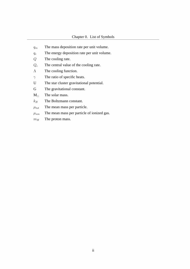
Chapter 0. List of Symbols

qm The mass deposition rate per unit volume.

qe The energy deposition rate per unit volume.

Q The cooling rate.

Qc The central value of the cooling rate.

Λ The cooling function.

γ The ratio of specific heats.

U The star cluster gravitational potential.

G The gravitational constant.

M⊙ The solar mass.

kB The Boltzmann constant.

µtot The mean mass per particle.

µion The mean mass per particle of ionized gas.

mH The proton mass.

ii

Contents

List of Symbols i

Contents iii

1 Introduction 1

1.1 Observations of super star clusters . . . . . . . . . . . . . . . . .. . . 1

1.2 The Star Cluster Driven Wind Theory . . . . . . . . . . . . . . . . . . 3

1.3 Aim of the Thesis . . . . . . . . . . . . . . . . . . . . . . . . . . . . . 5

1.4 Structure of the Thesis . . . . . . . . . . . . . . . . . . . . . . . . . . 6

2 The Star Cluster Model 9

2.1 Star Cluster Model . . . . . . . . . . . . . . . . . . . . . . . . . . . . 9

2.2 The Star Cluster Escape Velocity . . . . . . . . . . . . . . . . . . . . .12

2.3 An Exponentialversusa King Stellar Density Distribution . . . . . . . 13

3 The Star Cluster Wind Model 17

3.1 Main Hydrodynamic Equations . . . . . . . . . . . . . . . . . . . . . . 17

4 Methodology for solving the Boundary-Value Problem 21

4.1 Topology of the Integral Curves . . . . . . . . . . . . . . . . . . . . . 21

4.2 The Initial Conditions at the star cluster center . . . . . . .. . . . . . . 24

4.3 The Boundary Conditions . . . . . . . . . . . . . . . . . . . . . . . . . 26

5 Results from the Calculations 33

iii

Contents

5.1 Comparison with previous results . . . . . . . . . . . . . . . . . . . .. 33

5.2 The Reference Model . . . . . . . . . . . . . . . . . . . . . . . . . . . 35

5.3 The Quasi-Adiabatic Regime . . . . . . . . . . . . . . . . . . . . . . . 36

5.4 The Catastrophic Cooling Regime . . . . . . . . . . . . . . . . . . . . 38

6 Concluding Remarks 47

Appendices 51

A The Derivative of the Wind Density 51

B The Derivative of the Local Sound Speed 53

C The Approximate Relations 55

D The Isothermal Wind Hydrodynamic Equations 57

Figure Index 59

Table Index 61

References 63

iv

Chapter 1

Introduction

Super star clusters (SSCs) are high-density coeval young stellar systems which contain

between105− 107 M⊙ within a radius of few parsecs (∼ 1− 10 pc) (Whitmore, 2000).

They are usually found in systems with an intense mode of starformation, such as the

most luminous HII and starburst galaxies (Meurer et al., 1995; O’Connell et al., 1994;

Whitmore & Schweizer, 1995; Johnson et al., 2000, and references therein).

SSCs drive powerful winds formed by the thermalization of thekinetic energy sup-

plied by massive stars and high velocity supernova explosions. Moreover, it is nowa-

days recognized that most of stars, if not all of them, are formed in clustered environ-

ments (Lada & Lada, 2003) resulting in a combined effect of winds of many stars. This

combined effect can drive galactic-scale winds which affect the evolution of the host

galaxy itself and its surroundings (Heckman et al., 1990).

In sections1.1 and 1.2 I briefly review the main observations of star clusters and

the major contributions regarding the hydrodynamics of star cluster driven winds. In

section 1.3, I present the objectives of this thesis.

1.1 Observations of super star clusters

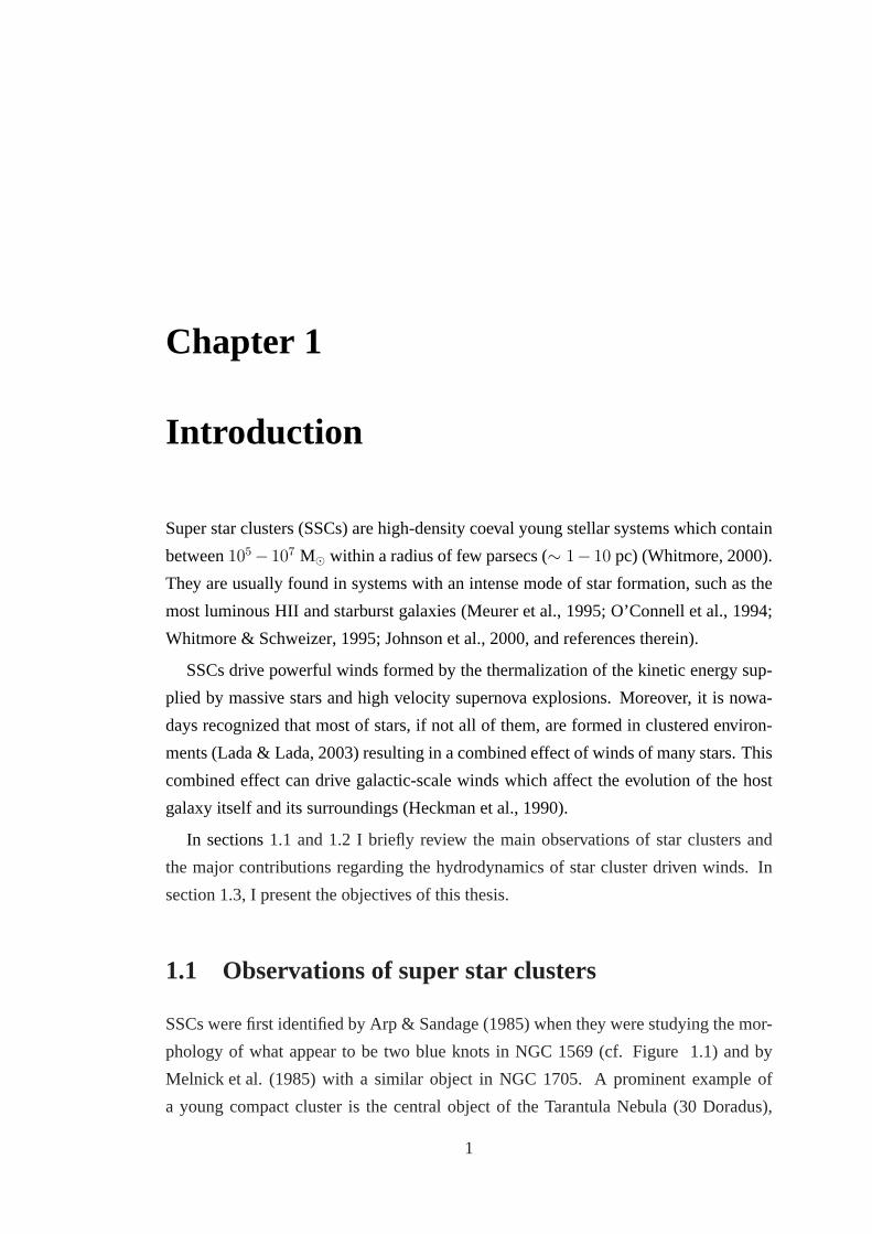
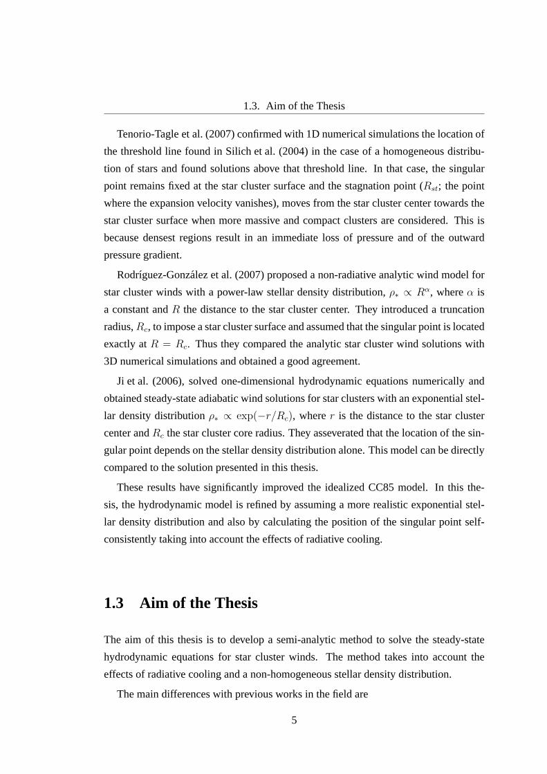
SSCs were first identified by Arp & Sandage (1985) when they werestudying the mor-

phology of what appear to be two blue knots in NGC 1569 (cf. Figure 1.1) and by

Melnick et al. (1985) with a similar object in NGC 1705. A prominent example of

a young compact cluster is the central object of the Tarantula Nebula (30 Doradus),

1

Chapter 1. Introduction

Figure 1.1: HST image of NGC 1569. The image exhibits two prominent blue star clustersexperiencing intense episodes of star formation. Image credit: NASA, ESA& P. Anders.

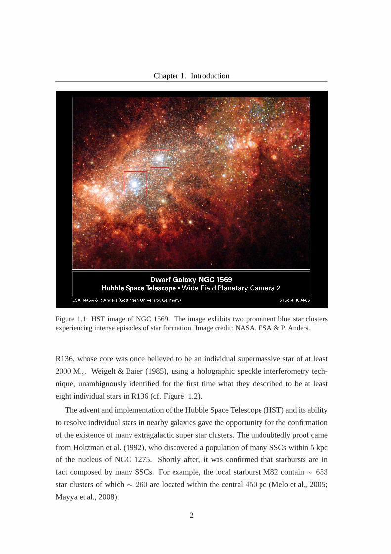
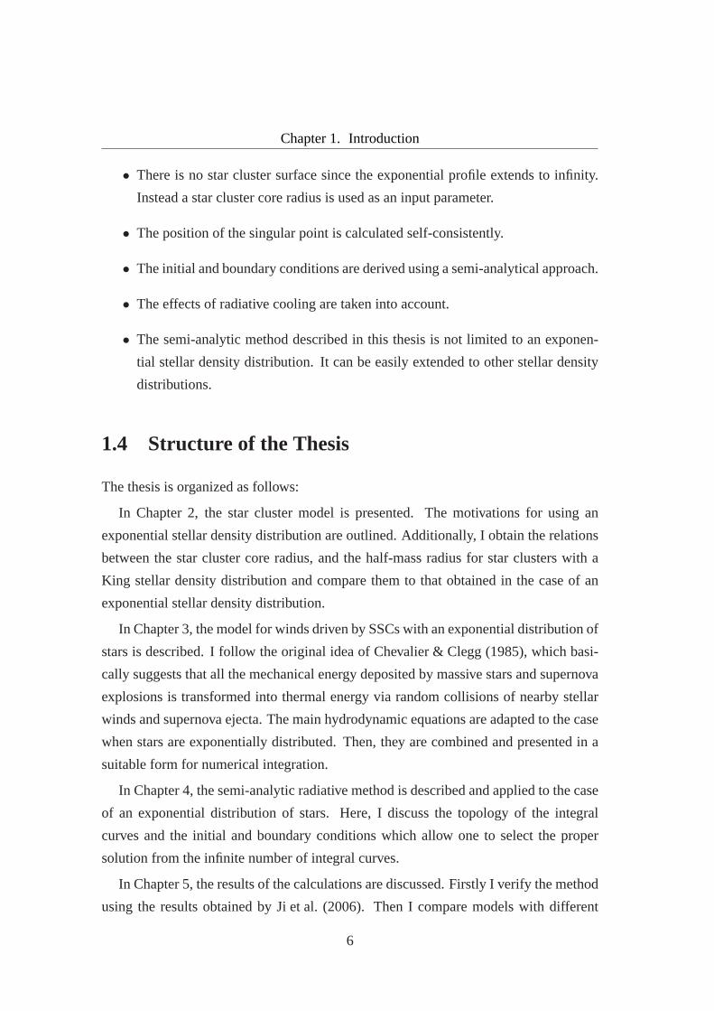
R136, whose core was once believed to be an individual supermassive star of at least

2000 M⊙. Weigelt & Baier (1985), using a holographic speckle interferometry tech-

nique, unambiguously identified for the first time what they described to be at least

eight individual stars in R136 (cf. Figure 1.2).

The advent and implementation of the Hubble Space Telescope(HST) and its ability

to resolve individual stars in nearby galaxies gave the opportunity for the confirmation

of the existence of many extragalactic super star clusters.The undoubtedly proof came

from Holtzman et al. (1992), who discovered a population of many SSCs within5 kpc

of the nucleus of NGC 1275. Shortly after, it was confirmed that starbursts are in

fact composed by many SSCs. For example, the local starburst M82 contain∼ 653

star clusters of which∼ 260 are located within the central450 pc (Melo et al., 2005;

Mayya et al., 2008).

2

1.2. The Star Cluster Driven Wind Theory

Figure 1.2: HST image of the R136 Cluster in the center of 30 Doradus. R136a was originallythought to be a supermassive star. Image credit: HST/NASA/ESA.

The typical sizes of SSCs (also called young star clusters) ofabout∼ 1 − 10 pc,

resemble those of the old Galactic globular clusters. Estimates of cluster ages have

shown that SSCs are usually older than their crossing times, indicating that they are

gravitationally bound (McCrady et al., 2003).

The radial profiles of young star clusters are best reproduced by King models (King,

1962; Mengel et al., 2002) derived for globular clusters. Ithas been suggested that at

least a small fraction of SSCs could survive and eventually become nowadays globular

clusters (Billett et al., 2001; Portegies Zwart et al., 2010).

1.2 The Star Cluster Driven Wind Theory

Star cluster winds are important in interstellar astrophysics because they affect the evo-

lution of the surrounding interstellar medium, enrich it with the products of massive

stars evolution and may result in triggering subsequent star formation.

The physical processes which drive star cluster winds are different from those which

drive winds from individual stars. Winds from individual stars are formed due to radi-

ation pressure absorbed in the outer layers of stars. Instead, Chevalier & Clegg (1985,

3

Chapter 1. Introduction

hereafter CC85) proposed that star cluster winds are formed due to the efficient thermal-

ization of the kinetic energy caused by random collisions ofgas ejected by supernova

explosions and stellar winds. This produces a large centraloverpressure that allows the

reinserted matter to accelerate and form strong outflows, the star cluster winds.

CC85 presented an analytical solution for winds driven by starbursts with radiusRsc

and uniform mass and energy deposition rates. Canto et al. (2000) compared the CC85

analytic predictions with winds generated by discrete stars (with a mean separation

of 0.1 pc) assuming much larger ranges of temperatures and densities than the CC85

model. They also carried out numerical simulations and found that the analytic solution

and the numerical results are in a reasonable agreement. These adiabatic models predict

the existence of extended X-ray envelopes that could be observationally detected.

In these models, the expansion velocity grows rapidly from zero km s−1 at the star

cluster center to the sound speed at the star cluster surfaceRsc. Thus, inside the star

cluster, the density, pressure and temperature of the wind remain almost uniform. How-

ever, outsideRsc, the hydrodynamical properties of the resultant wind outflow (the run

of density, temperature and expansion velocity), asymptotically approachρw ∼ r−1/2,

Tw ∼ r−4/3 anduw ∼ uA∞, whereuA∞ is the adiabatic wind terminal velocity.

Silich et al. (2004) presented a self-consistent stationary semi-analytic solution for

spherically symmetric winds driven by massive homogeneousstar clusters which in-

cludes radiative cooling. They found that radiative cooling maychange significantly

the temperature distribution of the windin the case of very massive and compact star

clusters. They found a threshold line in the planeLsc vs. Rsc (whereLsc is the mechan-

ical luminosity), above which the stationary wind solutionis inhibited.

Additionally, they discussed the solution topology for thehydrodynamic equations.

In their model, there are three possible types of integral curves corresponding to differ-

ent possible positions of the singular point with respect tothe star cluster surface: the

stationary wind solution in which the singular point is located at the star cluster surface

and the flow is subsonic inside and supersonic outside the star cluster. The breeze solu-

tion in which the central temperature is smaller than in the stationary wind solution; the

maximum value of the outflow velocity is shifted outside the star cluster and the flow

is subsonic everywhere. The unphysical double valued solution in which the central

temperature is larger than in the stationary wind case.

4

1.3. Aim of the Thesis

Tenorio-Tagle et al. (2007) confirmed with 1D numerical simulations the location of

the threshold line found in Silich et al. (2004) in the case ofa homogeneous distribu-

tion of stars and found solutions above that threshold line.In that case, the singular

point remains fixed at the star cluster surface and the stagnation point (Rst; the point

where the expansion velocity vanishes), moves from the starcluster center towards the

star cluster surface when more massive and compact clustersare considered. This is

because densest regions result in an immediate loss of pressure and of the outward

pressure gradient.

Rodrıguez-Gonzalez et al. (2007) proposed a non-radiative analytic wind model for

star cluster winds with a power-law stellar density distribution, ρ∗ ∝ Rα, whereα is

a constant andR the distance to the star cluster center. They introduced a truncation

radius,Rc, to impose a star cluster surface and assumed that the singular point is located

exactly atR = Rc. Thus they compared the analytic star cluster wind solutions with

3D numerical simulations and obtained a good agreement.

Ji et al. (2006), solved one-dimensional hydrodynamic equations numerically and

obtained steady-state adiabatic wind solutions for star clusters with an exponential stel-

lar density distributionρ∗ ∝ exp(−r/Rc), wherer is the distance to the star cluster

center andRc the star cluster core radius. They asseverated that the location of the sin-

gular point depends on the stellar density distribution alone. This model can be directly

compared to the solution presented in this thesis.

These results have significantly improved the idealized CC85 model. In this the-

sis, the hydrodynamic model is refined by assuming a more realistic exponential stel-

lar density distribution and also by calculating the position of the singular point self-

consistently taking into account the effects of radiative cooling.

1.3 Aim of the Thesis

The aim of this thesis is to develop a semi-analytic method tosolve the steady-state

hydrodynamic equations for star cluster winds. The method takes into account the

effects of radiative cooling and a non-homogeneous stellardensity distribution.

The main differences with previous works in the field are

5

Chapter 1. Introduction

• There is no star cluster surface since the exponential profile extends to infinity.

Instead a star cluster core radius is used as an input parameter.

• The position of the singular point is calculated self-consistently.

• The initial and boundary conditions are derived using a semi-analytical approach.

• The effects of radiative cooling are taken into account.

• The semi-analytic method described in this thesis is not limited to an exponen-

tial stellar density distribution. It can be easily extended to other stellar density

distributions.

1.4 Structure of the Thesis

The thesis is organized as follows:

In Chapter 2, the star cluster model is presented. The motivations for using an

exponential stellar density distribution are outlined. Additionally, I obtain the relations

between the star cluster core radius, and the half-mass radius for star clusters with a

King stellar density distribution and compare them to that obtained in the case of an

exponential stellar density distribution.

In Chapter 3, the model for winds driven by SSCs with an exponential distribution of

stars is described. I follow the original idea of Chevalier & Clegg (1985), which basi-

cally suggests that all the mechanical energy deposited by massive stars and supernova

explosions is transformed into thermal energy via random collisions of nearby stellar

winds and supernova ejecta. The main hydrodynamic equations are adapted to the case

when stars are exponentially distributed. Then, they are combined and presented in a

suitable form for numerical integration.

In Chapter 4, the semi-analytic radiative method is described and applied to the case

of an exponential distribution of stars. Here, I discuss thetopology of the integral

curves and the initial and boundary conditions which allow one to select the proper

solution from the infinite number of integral curves.

In Chapter 5, the results of the calculations are discussed. Firstly I verify the method

using the results obtained by Ji et al. (2006). Then I comparemodels with different

6

1.4. Structure of the Thesis

input parameters to a reference model. The impact of radiative cooling is then discussed

emphasizing the main differences with adiabatic and quasi-adiabatic wind regimes.

Finally, in Chapter6, I briefly summarize the main results and outline a number of

possible extensions to this work.

7

Chapter 2

The Star Cluster Model

In this chapter the star cluster model is formulated. In contrast with most previous

works in the field, the stars are not homogeneously distributed inside a star cluster

surface but follow an exponential distribution. In section2.1, I obtain the relations

between the star cluster core radius, and the half-mass radius for star clusters with a

King stellar density distribution and compare them to that obtained in the case of an

exponential stellar density distribution. Additionally,, the star cluster escape velocity is

compared, in section 2.2, to the sound speed in order to justify why I do not take into

consideration the gravitational pull of the star cluster and tidal forces. In section 2.3 the

motivations for using an exponential stellar density distribution are outlined.

2.1 Star Cluster Model

A young (≤ 40 Myr), compact stellar cluster with total massMsc and no-time depen-

dent parameters is considered.

It is also assumed that

• The star cluster is spherically symmetric;

• The stellar mass density distribution is an exponential function with respect to

the distance to the star cluster center

ρ∗(r) = ρ∗oe−r/Rc , (2.1)

9

Chapter 2. The Star Cluster Model

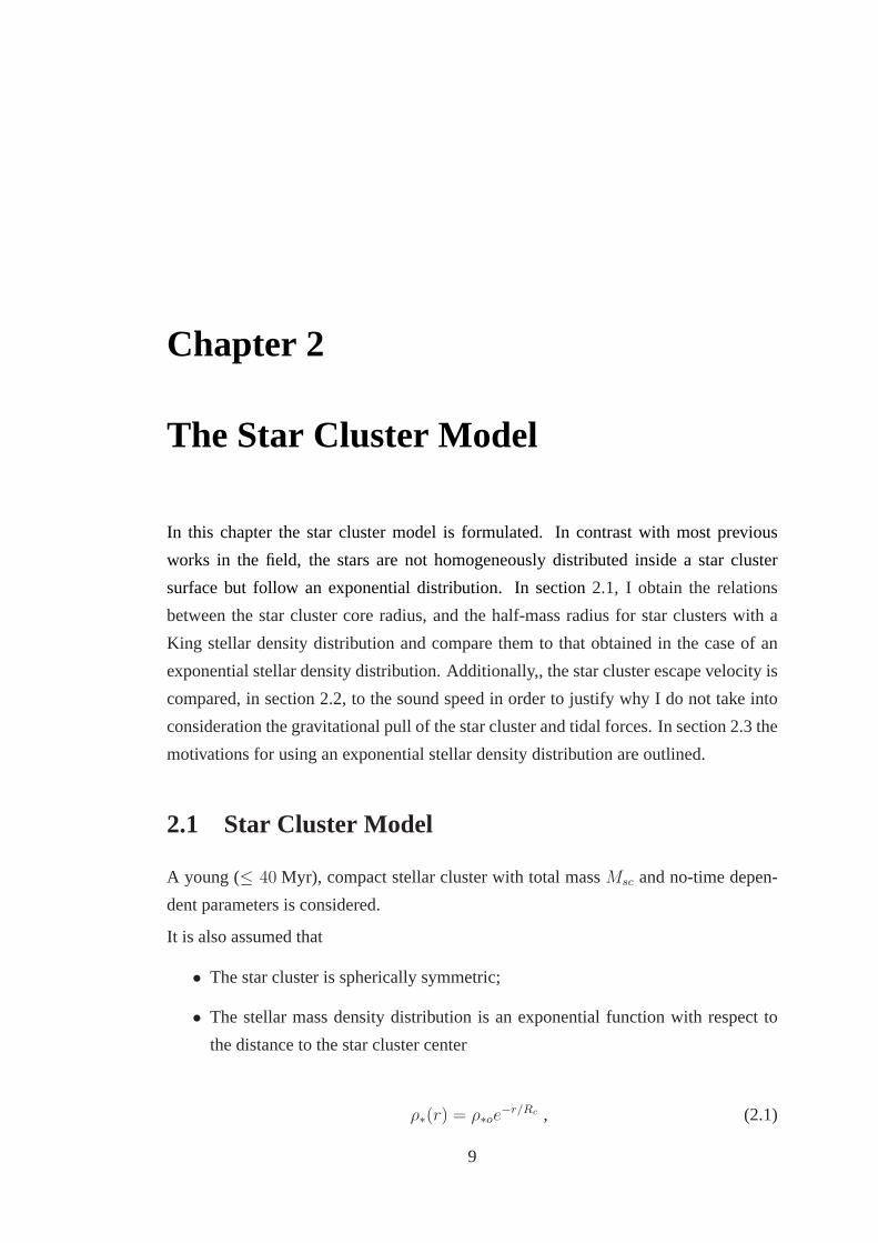
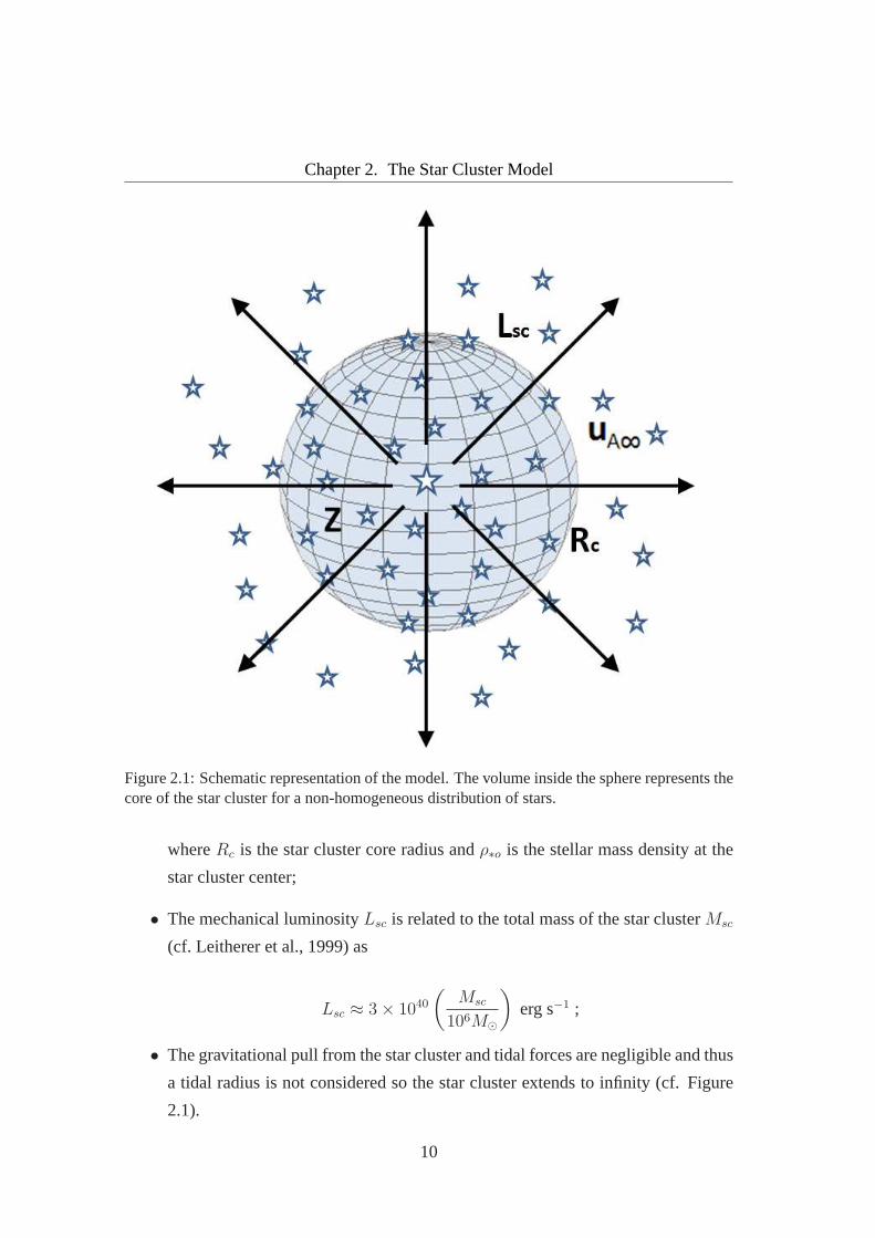
Figure 2.1: Schematic representation of the model. The volume inside the sphere represents thecore of the star cluster for a non-homogeneous distribution of stars.

whereRc is the star cluster core radius andρ∗o is the stellar mass density at the

star cluster center;

• The mechanical luminosityLsc is related to the total mass of the star clusterMsc

(cf. Leitherer et al., 1999) as

Lsc ≈ 3× 1040(

Msc

106M⊙

)

erg s−1 ;

• The gravitational pull from the star cluster and tidal forces are negligible and thus

a tidal radius is not considered so the star cluster extends to infinity (cf. Figure

2.1).

10

2.1. Star Cluster Model

The two parameters,Lsc andMsc, are related by the equation

Lsc =1

2Mscu

2

A∞ (2.2)

whereuA∞ is the adiabatic wind terminal velocity. I will useuA∞ as the input parame-

ter of the model instead ofMsc for all the calculations.

The massM(r) at any distance from the star cluster center can be found by integration

M(r) = 4π

∫ r

0

ρ∗(r)r2dr = Msc

[

1−

(

1 +r

Rc

+1

2

r2

R2c

)

e−r/Rc

]

, (2.3)

where the total mass of the star cluster is

Msc =

∫ ∞

0

4πr2ρ∗(r)dr = 8πρ∗oR3

c . (2.4)

Note that terms in the bracket,

(

1 +r

Rc

+1

2

r2

R2c

)

, coincide with the first three terms

of the Taylor series around zero for the exponential function er/Rc.

The stellar mass density at any distance to the star cluster center is then

ρ∗(r) =Msc

8πR3c

e−r/Rc . (2.5)

The difference between the exponential and homogeneous distributions is that in the

exponential case the star cluster does not have an edge. Nevertheless, the total mass of

the star cluster is finite.

Equation (2.3) allows to calculate the relation between thehalf-mass radiusRHM and

the star cluster core radius

RHM/Rc ≈ 2.66 , (2.6)

Thus the half mass radius is larger than the star cluster coreradius by a factor of2.66.

This relation is important in order to compare models with different stellar density

distributions whe the star clusters have the same half-massradius.

11

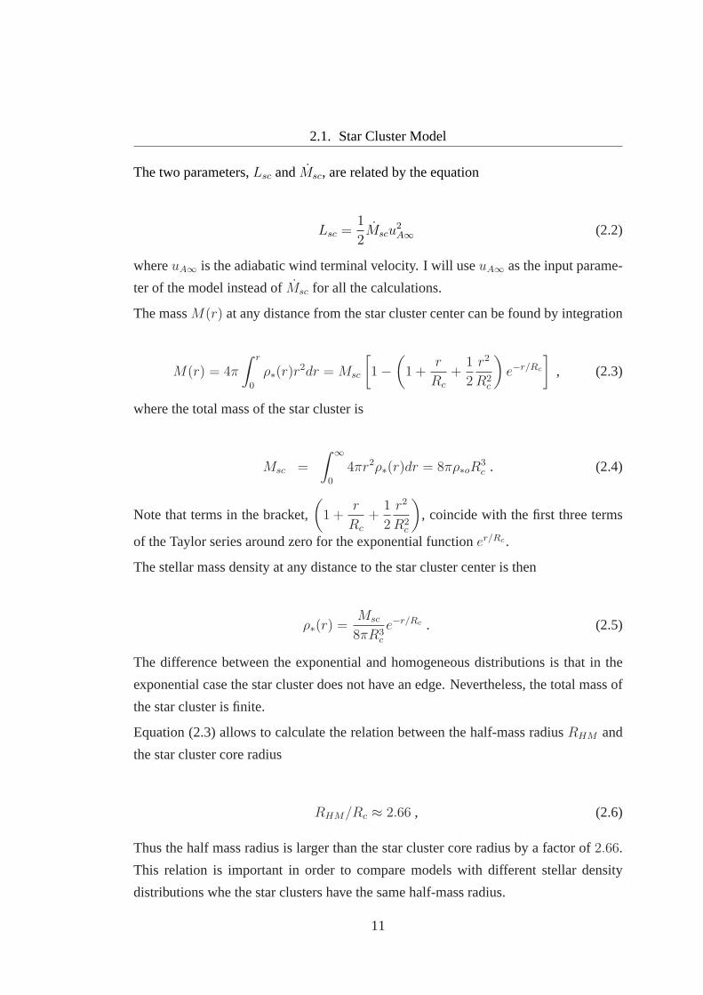
Chapter 2. The Star Cluster ModelSpeed (km s

-1 )

0

100

200

300

400

500

600

R(pc)0 20 40 60 80 100

Escape Velocity

Sound Speed

Figure 2.2: Comparison between the adiabatic sound speed (solid line) and the escape velocity(dashed line) of the star cluster. The total mass of the star cluster is assumedto beMsc =106 M⊙, the adiabatic wind terminal velocity isuA∞ = 1000 km s−1 and the star cluster coreradius isRc = 1 pc.

2.2 The Star Cluster Escape Velocity

In the case of an extended star cluster, the escape velocityvesc is defined by the equation

(Clarke & Carswell, 2007)

v2esc = −2U = 2G

∫ ∞

r

M(r)dr

r2, (2.7)

whereU is the gravitational potential of the star cluster andG is the gravitational con-

stant. Substituting equation (2.3) into (2.7), the escape velocity from the star cluster

with an exponential stellar density distribution is then

v2esc = 2GMsc

[

−1

r+

e−r/Rc

r+

∫ ∞

r

e−r/Rc

rRc

−

∫ ∞

r

e−r/Rc

rRc

+e−r/Rc

2Rc

] ∣

∣

∣

∣

∞

r

(2.8)

12

2.3. An Exponentialversusa King Stellar Density Distribution

Thus the escape velocity for star clusters with an exponential stellar density distribution

is then

vesc =

√

2GMsc

[

1

r(1− e−r/Rc)−

e−r/Rc

2Rc

]

(2.9)

I do not take into consideration the gravitational pull of the star cluster and tidal

forces because the sound speed of the shocked gas at a given radius is usually much

higher than the corresponding star cluster escape velocity. Figure 2.2 compares the

sound speed in the star cluster wind with the star cluster escape velocity when the mass

of the star cluster isMsc = 106 M⊙, the adiabatic wind terminal velocity isuA∞ =

1000 km s−1 and the star cluster core radius isRc = 1 pc.

2.3 An Exponential versusa King Stellar Density Dis-

tribution

Mengel et al. (2002) observed a sample of super star clustersin theAntennaegalaxies

and found that the best fitting model for the light profiles of star clusters is a King

model (King, 1962). Then they assumed that the light distribution follows the mass

distribution and concluded that the effective radii of starclusters are approximately

4 pc, similar to what Whitmore et al. (1999) estimated as the average radius of the

stellar clusters in theAntennae.

I adopt exponential profiles instead of King profiles becausea King profile implies

an infinite total mass if one does not account for a tidal radius. This problem does

not occur if one assumes an exponential profile. Moreover, the exponential profile is

algebraically easier to deal with. Note that the model presented in this work can be

easily extended to the case of modified King profiles which have been proposed by

Elson et al. (1987, hereafter EFF)

ρ∗(r) =ρ∗o

[

1 +(

rRk

)2]α (2.10)

13

Chapter 2. The Star Cluster Modelρ*(M

Θ pc-3)

0

104

2·104

3·104

4·104

R(pc)0 2 4 6 8 10

EFF Profile with α=2

Exponential Profile

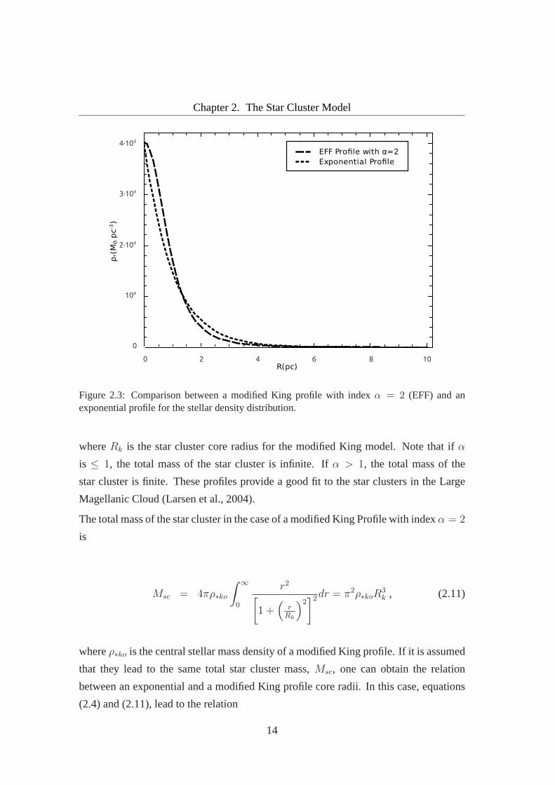
Figure 2.3: Comparison between a modified King profile with indexα = 2 (EFF) and anexponential profile for the stellar density distribution.

whereRk is the star cluster core radius for the modified King model. Note that ifα

is ≤ 1, the total mass of the star cluster is infinite. Ifα > 1, the total mass of the

star cluster is finite. These profiles provide a good fit to the star clusters in the Large

Magellanic Cloud (Larsen et al., 2004).

The total mass of the star cluster in the case of a modified KingProfile with indexα = 2

is

Msc = 4πρ∗ko

∫ ∞

0

r2[

1 +(

rRk

)2]2

dr = π2ρ∗koR3

k , (2.11)

whereρ∗ko is the central stellar mass density of a modified King profile.If it is assumed

that they lead to the same total star cluster mass,Msc, one can obtain the relation

between an exponential and a modified King profile core radii.In this case, equations

(2.4) and (2.11), lead to the relation

14

2.3. An Exponentialversusa King Stellar Density Distribution

Rk =

√

8ρ∗oπρ∗ko

Rc . (2.12)

When the central stellar mass densities,ρ∗o andρ∗ko are also equal, equation (2.12)

yields

Rk =

√

8

πRc ≈ 1.365Rc. (2.13)

Thus in the case of the modified King profile withα = 2, the star cluster core radius

Rk is larger than in the exponential case within a factor ofRk ≈ 1.365Rc. Figure 2.3

compares the adopted exponential and modified King profiles in the case when the total

mass of the star cluster isMsc = 106M⊙.

15

Chapter 3

The Star Cluster Wind Model

In this chapter, the model for winds driven by SSCs with an exponential distribution of

stars is constructed. The main hydrodynamic equations are adapted to the case when

stars are exponentially distributed. Then, they are combined and presented in a suitable

form for numerical integration.

3.1 Main Hydrodynamic Equations

Steady state spherically symmetric hydrodynamic equations which take into consid-

eration the energy and mass continuously deposited to the flow (see, for example

Johnson & Axford, 1971; Chevalier & Clegg, 1985; Canto et al., 2000; Silich et al., 2004;

Ji et al., 2006, and references therein) are

1

r2d

dr(ρwuwr

2) = qm , (3.1)

ρwuwduw

dr= −

dPw

dr− qmuw , (3.2)

1

r2d

dr

[

ρwuwr2

(

1

2u2

w +γ

γ − 1

Pw

ρw

)]

= qe −Q . (3.3)

17

Chapter 3. The Star Cluster Wind Model

wherePw, uw, andρw are the thermal pressure, the velocity and the density of the

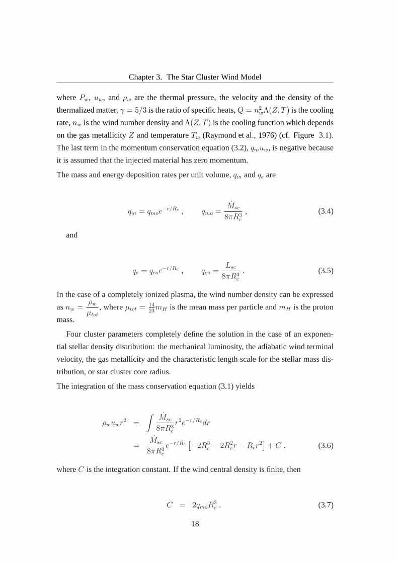
thermalized matter,γ = 5/3 is the ratio of specific heats,Q = n2

wΛ(Z, T ) is the cooling

rate,nw is the wind number density andΛ(Z, T ) is the cooling function which depends

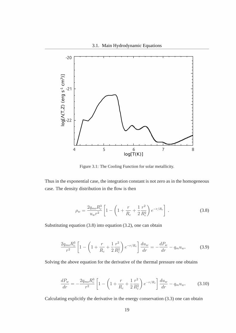
on the gas metallicityZ and temperatureTw (Raymond et al., 1976) (cf. Figure3.1).

The last term in the momentum conservation equation (3.2),qmuw, is negative because

it is assumed that the injected material has zero momentum.

The mass and energy deposition rates per unit volume,qm andqe are

qm = qmoe−r/Rc , qmo =

Msc

8πR3c

, (3.4)

and

qe = qeoe−r/Rc , qeo =

Lsc

8πR3c

. (3.5)

In the case of a completely ionized plasma, the wind number density can be expressed

asnw =ρwµtot

, whereµtot =14

23mH is the mean mass per particle andmH is the proton

mass.

Four cluster parameters completely define the solution in the case of an exponen-

tial stellar density distribution: the mechanical luminosity, the adiabatic wind terminal

velocity, the gas metallicity and the characteristic length scale for the stellar mass dis-

tribution, or star cluster core radius.

The integration of the mass conservation equation (3.1) yields

ρwuwr2 =

∫

Msc

8πR3c

r2e−r/Rcdr

=Msc

8πR3c

e−r/Rc[

−2R3

c − 2R2

cr −Rcr2]

+ C . (3.6)

whereC is the integration constant. If the wind central density is finite, then

C = 2qmoR3

c . (3.7)

18

3.1. Main Hydrodynamic Equations

log[Λ(T,Z) (erg s

-1 cm

3)]

-22

-21

-20

log[T(K)]4 5 6 7 8

Figure 3.1: The Cooling Function for solar metallicity.

Thus in the exponential case, the integration constant is not zero as in the homogeneous

case. The density distribution in the flow is then

ρw =2qmoR

3

c

uwr2

[

1−

(

1 +r

Rc

+1

2

r2

R2c

)

e−r/Rc

]

. (3.8)

Substituting equation (3.8) into equation (3.2), one can obtain

2qmoR3

c

r2

[

1−

(

1 +r

Rc

+1

2

r2

R2c

)

e−r/Rc

]

duw

dr= −

dPw

dr− qmuw. (3.9)

Solving the above equation for the derivative of the thermalpressure one obtains

dPw

dr= −

2qmoR3

c

r2

[

1−

(

1 +r

Rc

+1

2

r2

R2c

)

e−r/Rc

]

duw

dr− qmuw. (3.10)

Calculating explicitly the derivative in the energy conservation (3.3) one can obtain

19

Chapter 3. The Star Cluster Wind Model

1

r2d

dr

[

ρwuwr2

(

1

2u2

w +c2s

γ − 1

)]

= qm

{

u2

w

2+

c2sγ − 1

}

+ ρwuw

{

uwduw

dr+

d

dr

c2sγ − 1

}

= qe −Q, (3.11)

wherecs is the local sound speed given byc2s =γkBµion

Tw = γPw

ρw, kB is the Boltzmann

constant andµion = 14

11mH is the total mean mass per particle of the ionized gas in

terms of the hydrogen mass.

Combining equation (3.11) with equations (3.1), (3.8) and (3.2), one can obtain

qe −Q = ρwu2

w

duw

dr+

u2

w

2qm

+γ

γ − 1

{

ρw

(

c2sγ

− u2

w

)

duw

dr− qmu

2

w +4qmoR

3

c

r3Pw

ρw

[

1−

(

1 +r

Rc

+1

2

r2

R2c

)

e−r/Rc

]}

.

(3.12)

When one multiplies both sides of equation (3.12) by(γ − 1), one can express the

change of the wind velocity with respect to the distance to the star cluster center as

duw

dr=

(γ − 1)(qe −Q)−4qmoR

3

cc2

s

r3(1− e−r/Rc) + qm

[

u2

w

2(γ + 1) + 4

R3

c

r3

(

r

Rc

+1

2

r2

R2c

)

c2s

]

ρw(c2

s − u2

w).

(3.13)

Equations (3.8), (3.10) and (3.13) are more suitable for numerical integration than equa-

tions (3.1), (3.2) and (3.3). In the next chapter, the methodology for solving them is

presented.

20

Chapter 4

Methodology for solving the

Boundary-Value Problem

In this chapter, a semi-analytic method for solving the hydrodynamic equations formu-

lated in the preceding chapter is developed. Firstly, in section 4.1 I discuss the topology

of the possible solutions of the differential equations (3.10) and (3.13). Then in sections

4.2 and 4.3 I discuss the initial and boundary conditions which allow one to select the

proper solution from the infinite number of integral curves.The proper solution is the

only solution which passes through the singular point,i.e. the point at which the wind

becomes supersonic. The procedure for solving the problem uses three integrations:

one from the star cluster center outwards, one from the singular point inwards and one

starting at the singular point outwards.

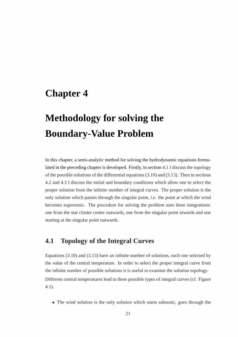
4.1 Topology of the Integral Curves

Equations (3.10) and (3.13) have an infinite number of solutions, each one selected by

the value of the central temperature. In order to select the proper integral curve from

the infinite number of possible solutions it is useful to examine the solution topology.

Different central temperatures lead to three possible types of integral curves (cf. Figure

4.1).

• The wind solution is the only solution which starts subsonic, goes through the

21

Chapter 4. Methodology for solving the Boundary-Value Problemu(km s

-1)

0

200

400

600

800

1000

R(pc)0 1 2 3 4 5

Wind

N

D

RN RD Rsp

Figure 4.1: Types of integral curves for the differential equation (3.13). The solid line corre-sponds to the wind solution. The thin dashed line corresponds to theN -type solution and thethick dashed line corresponds to theD-type solution.

singular point,Rsp, where the numerator and the denominator of equation (3.13)

change their sign simultaneously, and then reaches supersonic values farther out-

wards. Notice, that the central temperature which leads to the wind solution must

be selected with high accuracy.

• TheN -type solution occurs when the central temperature is lowerthan in the

wind solution. In this case, the solution remains subsonic everywhere. The

change of sign in equation (3.13) only takes place in the numerator. The out-

flow velocity reaches its maximum value at a radiusRN from the star cluster

center and then decreases with increasing radius from thereoff.

• TheD-type solution is an unphysical double-valued solution which occurs when

the central temperature is greater than that for the wind solution. In this case

22

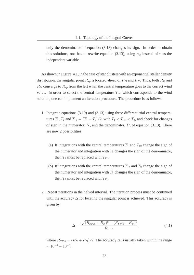
4.1. Topology of the Integral Curves

only the denominator of equation (3.13) changes its sign. In order to obtain

this solutions, one has to rewrite equation (3.13), usinguw instead ofr as the

independent variable.

As shown in Figure 4.1, in the case of star clusters with an exponential stellar density

distribution, the singular pointRsp is located ahead ofRD andRN . Thus, bothRD and

RN converge toRsp from the left when the central temperature goes to the correct wind

value. In order to select the central temperatureTwc which corresponds to the wind

solution, one can implement an iteration procedure. The procedure is as follows

1. Integrate equations (3.10) and (3.13) using three different trial central tempera-

turesT1, T2 andT12 = (T1 + T2)/2, with T1 < Twc < T2, and check for changes

of sign in the numerator,N , and the denominator,D, of equation (3.13). There

are now 2 possibilities

(a) If integrations with the central temperaturesT1 andT12 change the sign of

the numerator and integration withT2 changes the sign of the denominator,

thenT1 must be replaced withT12.

(b) If integrations with the central temperaturesT12 andT2 change the sign of

the numerator and integration withT1 changes the sign of the denominator,

thenT2 must be replaced withT12.

2. Repeat iterations in the halved interval. The iteration process must be continued

until the accuracy∆ for locating the singular point is achieved. This accuracy is

given by

∆ =

√

(RSPA −RN)2 + (RSPA −RD)2

RSPA

, (4.1)

whereRSPA = (RN +RD)/2. The accuracy∆ is usually taken within the range

∼ 10−4 − 10−3.

23

Chapter 4. Methodology for solving the Boundary-Value Problem

4.2 The Initial Conditions at the star cluster center

In order to start integrations, one has to select the velocity uw, the densityρw (or equiv-

alentlynw) and the temperatureTw at the star cluster center.

It looks like equations (3.8) and (3.13) have a singularity at the star cluster center.

However, this is not the case. Indeed, using the L’Hopital’s rule and the condition that

the wind central density must be finite, one can obtain the following limits

limr→0

uw =2qmo

ρwo

limr→0

R3

c

r2

[

1−

(

1 +r

Rc

+1

2

r2

R2c

)

e−r/Rc

]

= 0 . (4.2)

limr→0

duw

dr= lim

r→0

(γ − 1)(qe −Q)−4qmoR

3

cc2

s

r3(1− e−r/Rc) +

4qmR3

c

r3

(

r

Rc

+1

2

r2

R2c

)

c2s

ρwc2s

=(γ − 1)(qeo −Qc)−

2

3qmoc

2

c

ρwoc2c, (4.3)

whereqeo andQc are the central values for the energy deposition rate per unit volume

and the cooling rate, respectively. Besides this, one can obtain the relation between the

wind central density and the wind central temperature. Indeed the energy conservation

equation (3.11) leads to the relation

qe −Q = qm

[

u2

w

2+

c2sγ − 1

]

+ ρwuw

[

uwduw

dr+

d

dr

c2sγ − 1

]

, (4.4)

Taking into account that at the star cluster centeruw = 0 andduw

dris finite, one can

obtain

(γ − 1)(qeo −Qc) =

[

qmc2

s + ρwuwdc2sdr

] ∣

∣

∣

∣

r=0

, (4.5)

where the derivative of the sound speed with respect to the distance to the star cluster

center.

24

4.2. The Initial Conditions at the star cluster center

Substituting the derivative of the sound speeddc2sdr

(obtained in AppendixB) into (4.5)

and taking into account that at the star cluster center the termsγρwu2

w

duw

drandγu2

wqm

vanish, one can obtain

(γ − 1)(qeo −Qc) =

[

ρwc2

s

duw

dr+

2ρwuwc2

s

r

] ∣

∣

∣

∣

r=0

(4.6)

Equations (3.8) and (4.3) allow to calculate the value of thelast term of equation (4.6)

whenr → 0

2ρwoc2

c limr→0

uw

r= 2ρwoc

2

c

[

(γ − 1)(qeo −Qc)−2

3qmoc

2

c

ρwoc2c

]

(4.7)

which leads to

2ρwoc2

c limr→0

uw

r= 2(γ − 1)(qeo −Qc)−

4

3qmoc

2

c . (4.8)

and equation (4.6) turns into

qmoc2

c = (γ − 1)(qeo −Qc) . (4.9)

Taking into account thatQc = n2

woΛ(Tc, Z), one can finally obtain

qmoc2

c = (γ − 1)[qeo − n2

woΛ(Tc, Z)] , (4.10)

Equation (4.10) shows that the wind central densitynwo and the central temperature are

not independent as in the adiabatic case (Chevalier & Clegg, 1985; Raga et al., 2001),

but are related by the equation

nwo =

qeo −qmoc

2

cγ−1

Λ(Tc)

1/2

= q1/2mo

u2

A∞2

−c2cγ−1

Λ(Tc)

1/2

, (4.11)

25

Chapter 4. Methodology for solving the Boundary-Value Problem

wherecc is the sound speed at the star cluster center. Equation (4.11) is consistent with

the relation found by Sarazin & White (1987) from the energy conservation equation

in their cooling flow model and that found by Silich et al. (2004) for star clusters with

homogeneous stellar density distribution.

The term

[

u2

A∞

2−

c2cγ − 1

]

in equation (4.11) cannot be negative in order to have a

density with a physical meaning. This is why the central temperatureTc cannot exceed

the adiabatic wind value

Tmaxc =

(γ − 1)µionu2

A∞

2γkB. (4.12)

In order to start the numerical integration, one has to take asmall step away,∆R1, from

the star cluster center, and use as initial conditions

Rw = ∆R1 ,

uw = uwo +duw

dr

∣

∣

∣

∣

0

∆R1 ,

ρw =2qmoR

3

c

uwR2w

[

1−

(

1 +Rw

Rc

+1

2

R2

w

R2c

)

e−Rw/Rc

]

,

Pw = Pwo .

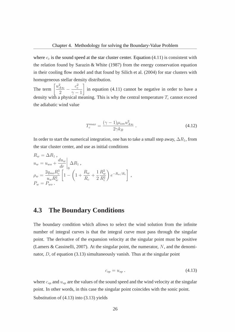
4.3 The Boundary Conditions

The boundary condition which allows to select the wind solution from the infinite

number of integral curves is that the integral curve must pass through the singular

point. The derivative of the expansion velocity at the singular point must be positive

(Lamers & Cassinelli, 2007). At the singular point, the numerator,N , and the denomi-

nator,D, of equation (3.13) simultaneously vanish. Thus at the singular point

csp = usp . (4.13)

wherecsp andusp are the values of the sound speed and the wind velocity at the singular

point. In other words, in this case the singular point coincides with the sonic point.

Substitution of (4.13) into (3.13) yields

26

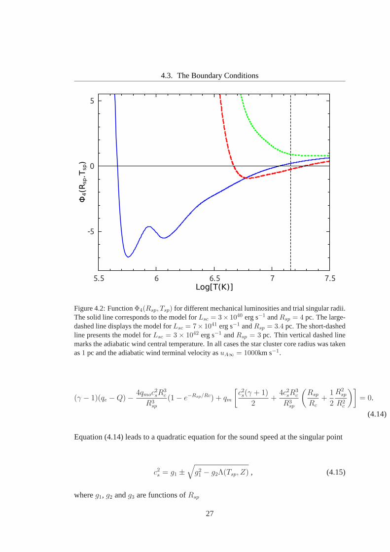
4.3. The Boundary ConditionsΦ

4(R

sp.T

sp)

-5

0

5

Log[T(K)]5.5 6 6.5 7 7.5

Figure 4.2: FunctionΦ4(Rsp, Tsp) for different mechanical luminosities and trial singular radii.The solid line corresponds to the model forLsc = 3× 1040 erg s−1 andRsp = 4 pc. The large-dashed line displays the model forLsc = 7× 1041 erg s−1 andRsp = 3.4 pc. The short-dashedline presents the model forLsc = 3 × 1042 erg s−1 andRsp = 3 pc. Thin vertical dashed linemarks the adiabatic wind central temperature. In all cases the star cluster core radius was takenas1 pc and the adiabatic wind terminal velocity asuA∞ = 1000km s−1.

(γ − 1)(qe −Q)−4qmoc

2

sR3

c

R3sp

(1− e−Rsp/Rc) + qm

[

c2s(γ + 1)

2+

4c2sR3

c

R3sp

(

Rsp

Rc

+1

2

R2

sp

R2c

)]

= 0.

(4.14)

Equation (4.14) leads to a quadratic equation for the sound speed at the singular point

c2s = g1 ±√

g21− g2Λ(Tsp, Z) , (4.15)

whereg1, g2 andg3 are functions ofRsp

27

Chapter 4. Methodology for solving the Boundary-Value Problem

g1 =γ − 1

4g3u2

A∞e−Rsp/Rc , (4.16)

g2 =4(γ − 1)qmoR

6

c

g3µ2

ionR4sp

[

1−

(

1 +Rsp

Rc

+1

2

R2

sp

R2c

)

e−Rsp/Rc

]2

,

(4.17)

and

g3 = 4

(

Rc

Rsp

)3(

1− e−Rsp/Rc)

−

[

(γ + 1)

2+ 4

(

Rc

Rsp

)2

+2Rc

Rsp

]

e−Rsp/Rc.

(4.18)

Equation (4.15) is a non-linear algebraic equation and it must be solved numerically. It

can be rewritten as

Φ4(Rsp, Tsp) = c4s − 2g1c2

s + g2Λ(Tsp, Z) = 0 , (4.19)

I solved equation (4.19) using a bisection scheme.

Figure 4.2 displays functionΦ4(Rsp, Tsp) for different values ofLsc in the case when

uA∞ = 1000 km s−1 andRc = 1 pc. This figure also shows that the functionΦ4(Rsp, Tsp)

may have one or two real roots belowTmaxc or no real roots.

Thus, one can obtain the temperature at the singular point using equation (4.19) if

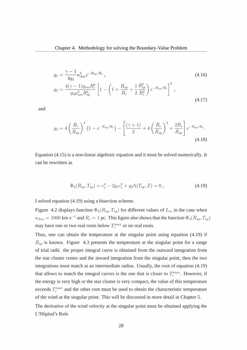
Rsp is known. Figure 4.3 presents the temperature at the singular point for a range

of trial radii. the proper integral curve is obtained from the outward integration from

the star cluster center and the inward integration from the singular point, then the two

integrations must match at an intermediate radius. Usually, the root of equation (4.19)

that allows to match the integral curves is the one that is closer toTmaxc . However, if

the energy is very high or the star cluster is very compact, the value of this temperature

exceedsTmaxc and the other root must be used to obtain the characteristic temperature

of the wind at the singular point. This will be discussed in more detail in Chapter 5.

The derivative of the wind velocity at the singular point must be obtained applying the

L’H opital’s Rule

28

4.3. The Boundary Conditionslog[T

sp(K)]

5

5.5

6

6.5

7

7.5

8

Rsp(pc)2 4 6 8

a)

log[T

sp(K)]

5

5.5

6

6.5

7

7.5

8

Rsp(pc)2 3 4 5 6 7

b)

log[T

sp(K)]

6

6.5

7

7.5

8

8.5

Rsp(pc)2 2.5 3 3.5 4 4.5 5

c)

log[T

sp(K)]

6

6.5

7

7.5

8

8.5

Rsp(pc)2.5 3

d)

Figure 4.3: The temperature at the singular pointversusthe trial singular radius. The terminalvelocity of the star cluster wind is assumed to be1000 km s−1 and the star cluster core radiusRc = 1pc. The solid line corresponds to the root that is closer toTmax

c in equation (4.19) andthe dashed line corresponds to the other root. Panel a) corresponds toMsc = 105M⊙, Panel b)toMsc = 106M⊙, Panel c) toMsc = 107M⊙ and Panel d) toMsc = 108M⊙.

limr→Rsp

duw

dr= lim

r→Rsp

∂N

∂Q

dQ

dr+

∂N

∂c2s

dc2sdr

+∂N

∂uw

duw

dr+

∂N

∂r

∂D

∂c2s

dc2sdr

+∂D

∂uw

duw

dr

. (4.20)

Here the derivatives are

∂N

∂Q

dQ

dr= −(γ − 1)

[

2Q

ρw

dρwdr

+Q

Λ

Tsp

c2s

µtot

µion

dΛ

dT

dc2sdr

]

, (4.21)

∂N

∂cs

dcsdr

=

[

−4qmoR

3

c

R3sp

(1− e−Rsp/Rsc) + 4qmR3

c

R3sp

(

Rsp

Rc

+1

2

R2

sp

R2c

)]

dc2sdr

, (4.22)

29

Chapter 4. Methodology for solving the Boundary-Value Problem

∂N

∂uw

duw

dr= (γ + 1)csqm , (4.23)

∂N

∂r= (1− γ)

qeRc

−1

2(γ + 1)qm

c2sRc

+12qmoR

3

cc2

s

R4sp

(1− e−Rsp/Rc)

−12qmR

2

cc2

s

R3sp

−6qmRcc

2

s

R2sp

−2qmc

2

s

Rsp

,

(4.24)

and

dD

dr=

∂D

∂c2s

dc2sdr

+∂D

∂uw

duw

dr=

dc2sdr

− 2csduw

dr. (4.25)

The derivatives of the wind density and the local sound speed(cf. Appendices A and

B) at the singular point are

dρwdr

= −duw

dr

ρwcs

+qmcs

−2ρwRsp

, (4.26)

and

dc2sdr

= −duw

dr(γ − 1)cs −

(γ + 1)csqmρw

+2c2sRsp

, (4.27)

respectively.

Equation (4.20) leads to a quadratic equation for the derivative of the wind velocity at

the singular point

− (γ + 1)csρw

(

duw

dr

)2

+

[

2c2sρwRsp

− (γ + 1)csqm

]

duw

dr= f1 + f2

[

−(γ + 1)csqm

ρw+

2c2sRsp

]

+duw

dr

[

2Q(γ − 1)

cs+

Q(γ − 1)2

Λ

Tsp

c2s

µtot

µion

dΛ

dT+ (γ + 1)csqm − (γ − 1)f2cs

]

+∂N

∂r,

(4.28)

30

4.3. The Boundary Conditions

where functionsf1 andf2 are

f1 = −(γ − 1)

{

2Qqmρwcs

−4Q

Rsp

−Q

Λ

(γ + 1)qmTsp

csρw

µtot

µion

dΛ

dT+

2QTsp

ΛRsp

dΛ

dT

}

, (4.29)

f2 = −4qmoR

3

c

R3sp

(1− e−Rsp/Rsc) + 4qmR3

c

R3sp

(

Rsp

Rc

+1

2

R2

sp

R2c

)

. (4.30)

Equation (4.28) has two solutions. One has to select the solution which results into

positive derivative of the wind velocity at the singular point

duw

dr=

a1 +√

a21+ 4aoa2

2a2, (4.31)

wherea0, a1 anda2 are

a0 = −

[

f1 + f2

[

−(γ + 1)csqm

ρw+

2c2sRsp

]

+∂N

∂r

]

,

a1 =2c2sρwRsp

− 2(γ + 1)csqm −2Q(γ − 1)

cs−

Q(γ − 1)2

Λ

Tsp

c2s

µtot

µion

dΛ

dT+ f2(γ − 1)cs ,

and

a2 = −(γ + 1)csρw .

The determination of the wind velocity gradient at the singular point allows one

to determine the analytic boundary conditions required to integrate the hydrodynamic

equations. It also allows a smooth transition through a region where the numerical

calculation is unstable as it may vary between large positive and negative values in a

short distance interval (Lamers & Cassinelli, 2007).

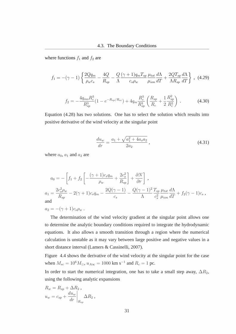
Figure 4.4 shows the derivative of the wind velocity at the singular point for the case

whenMsc = 106M⊙, uA∞ = 1000 km s−1 andRc = 1 pc.

In order to start the numerical integration, one has to take asmall step away,∆R2,

using the following analytic expansions

Rw = Rsp +∆R2 ,

uw = csp +duw

dr

∣

∣

∣

∣

Rsp

∆R2 ,

31

Chapter 4. Methodology for solving the Boundary-Value Problem

duw/dr (10-10 s-1)

0

1.5

2

Rsp(pc)2 2.5 3 3.5 4 4.5

Figure 4.4: The derivative of the wind velocity for different trial special point radii. The totalmass of the star cluster is assumed to beMsc = 106M⊙, terminal velocity1000 km s−1 and thestar cluster core radiusRc = 1 pc. This curve constrains the range of possible singular pointradii because only positive values of the derivative of the wind velocity are allowed for a wind.

ρw =2qmoR

3

c

uwR2w

[

1−

(

1 +Rw

Rc

+1

2

R2

w

R2c

)

e−Rw/Rc

]

,

dPw

dr= −ρwcsp

duw

dr

∣

∣

∣

∣

Rsp

−qmcsp ,

Pw = Psp +dPw

dr

∣

∣

∣

∣

Rsp

∆R2 .

The code employed for solving equations (3.10) and (3.13) uses the well-known inte-

grator called Stiff which applies the Adams’ Method. At eachstep of the integration,

Stiff automatically selects the step size of the integration according to the required ac-

curacy.

32

Chapter 5

Results from the Calculations

In this chapter, I present the results from the calculationsfor winds driven by SSCs

with an exponential stellar density distribution for a variety of input parameters using

the semi-analytic method described in the preceding chapter. For this purpose, I first

compare the runs of velocity and temperature obtained from semi-analytic radiative

calculations to the non-radiative numeric results from Ji et al. (2006). Then I define a

reference model, which represents a typical SSC. The distribution of the flow variables

(velocity, temperature, particle number density, thermalpressure and ram pressure)

obtained for thereference modelare then compared to those calculated in models with

other input parameters.

5.1 Comparison with previous results

Ji et al. (2006, hereafter JWK06) have considered numerically the case of super star

clusters with an exponential stellar density distribution. However, in their hydrody-

namic calculations they did not take into account the effects of radiative cooling. They

used the following input parameters: a star cluster core radius Rc = 0.48 pc, a mass

deposition rateMsc = 10−4 M⊙ yr−1 and three adiabatic wind terminal velocities

uA∞ = 500, 1000 and2000 km s−1 (from now on, JWK500, JWK1000 and JWK2000

cases, respectively).

In order to verify the semi-analytic method presented here,I carried out calculations

for the same input parameters. I usedLsc instead ofMsc as an input parameter using

33

Chapter 5. Results from the Calculations

log[T(K)]

5.0

6.0

7.0

8.0

R(pc)0 2 4 6 8 10

d)

log[T(K)]

5.0

6.0

7.0

8.0

R(pc)0 2 4 6 8 10

b)

u(km s

-1)

0

500

1000

1500

2000

R(pc)0 2 4 6 8 10

c)

u(km s

-1)

0

500

1000

1500

2000

R(pc)0 2 4 6 8 10

a)

Figure 5.1: The comparison of the semi-analytical radiative calculation to the numeric results ofJi et al. (2006). Short-dashed, solid and long-dashed lines presentthe results of the calculationsfor JWK500, JWK1000 and JWK2000, respectively. Panels a) and b)depict the runs of velocityand temperature obtained with the semi-analytic method. The vertical line marks thelocationof the singular point. I adapted panels c) and d) to show the results of the JWK06.

the relationLsc =1

2Mscu

2

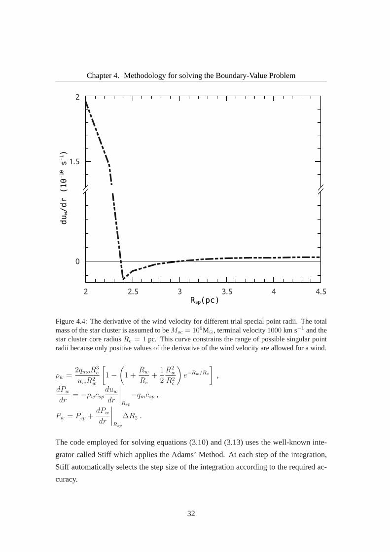
A∞. Figure 5.1 displays the results of these calculations (top

panels) and compare them to the results obtained by JWK06 (bottom panels). The two

methods are in excellent agreement. JWK obtained that the singular point is located

at Rsp = 1.97 pc. In the semi-analytic radiative wind calculations, the singular point

is located atRsp = 1.93 pc, Rsp = 1.93 pc andRsp = 1.94 pc, for the JWK500,

JWK1000 and JWK2000 cases, respectively.

34

5.2. The Reference Model

log[P(dyn cm

-2)]

-11

-10

-9

-8

-7

-6

R(pc)0 10 20 30 40 50

d)

log[T(K)]

5.5

6.0

6.5

7.0

R(pc)0 10 20 30 40 50

b)

log[n(cm

-3)]

-1

-0.5

0

0.5

1

1.5

2

2.5

3

R(pc)0 10 20 30 40 50

c)

u(km s

-1)

0

200

400

600

800

1000

R(pc)0 10 20 30 40 50

a)

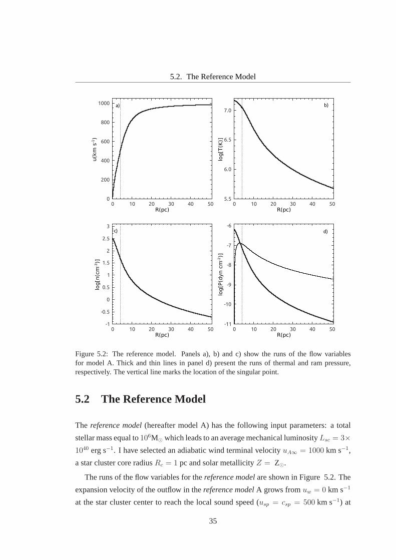
Figure 5.2: The reference model. Panels a), b) and c) show the runs ofthe flow variablesfor model A. Thick and thin lines in panel d) present the runs of thermal and ram pressure,respectively. The vertical line marks the location of the singular point.

5.2 The Reference Model

The reference model(hereafter model A) has the following input parameters: a total

stellar mass equal to106M⊙ which leads to an average mechanical luminosityLsc = 3×

1040 erg s−1. I have selected an adiabatic wind terminal velocityuA∞ = 1000 km s−1,

a star cluster core radiusRc = 1 pc and solar metallicityZ = Z⊙.

The runs of the flow variables for thereference modelare shown in Figure 5.2. The

expansion velocity of the outflow in thereference modelA grows fromuw = 0 km s−1

at the star cluster center to reach the local sound speed (usp = csp = 500 km s−1) at

35

Chapter 5. Results from the Calculations

the singular point atRsp = 4.04 pc (cf. Panela)). It continues then to grow rapidly

and reaches the terminal valuev∞ ∼ 990 km s−1. This velocity is slightly smaller than

the adiabatic wind terminal velocityuA∞. These two values would only coincide in the

absence of radiative cooling, because some fraction of the energy deposited in the flow

is radiated away.

The wind temperature decreases rapidly from its central valueTc ∼ 1.46 × 107 K

to Tsp ∼ 1.1 × 107 K at the singular point (cf. Panelb)). The particle number density

and the thermal pressure have rapid decays from their central values (cf. Panelsc) and

d)). The ram pressure,PRAM = ρwu2

w, and the thermal pressure are equal at a radius

RRAM ∼ 3 pc.

5.3 The Quasi-Adiabatic Regime

In this section, I compare the results obtained in the prior section to models with differ-

ent mechanical luminosities, star cluster core radii and adiabatic wind terminal veloci-

ties. The input parameters of each model are presented in Table 5.1.

Model Lsc(erg s−1) Rc(pc) uA∞(km s−1) Z(Z⊙)

A 3 ×1040 1.0 1000 1.0B 3×1039 1.0 1000 1.0C 3×1041 1.0 1000 1.0D 3×1040 0.2 1000 1.0E 3×1040 5.0 1000 1.0F 3×1040 1.0 750 1.0G 3×1040 1.0 2000 1.0

Table 5.1: Input parameters for models A, B, C, D, E, F and G.

In all these models, the outflow is quasi-adiabatic. This implies that the energy

carried away from the star cluster is small compared to the energy supplied by massive

stars and radiative cooling affects the flow at large or very large radii and therefore does

not affect the location of the singular point.

The runs of the flow variables for models A, B and C are shown in Figure 5.3.

In the case of model B, the outflow velocityuw equals the local sound speed,usp =

501.8 km s−1, atRsp = 4.04 pc (cf. Panela)). The wind temperature decreases from

36

5.3. The Quasi-Adiabatic Regime

the central valueTc ∼ 1.4× 107 K to Tsp ∼ 1.1× 107 K at the singular point (cf. Panel

b)). The density of the wind in model B is lower than in model A, byabout one order

of magnitude (cf. Panelc)). Indeed, combining equations (2.2), (3.4) and (3.8), one can

obtain

ρw =Lsc

2πuwu2

A∞r2

[

1−

(

1 +r

Rc

+1

2

r2

R2c

)

e−r/Rc

]

, (5.1)

Equation (5.1) shows that the wind density must grow whenLsc increases and de-

crease with increasinguA∞ andRc.

In model C, the density is approximately one order of magnitude higher than in

model A (cf. Panelc)). The singular point is located atRsp = 4.02 pc, where the

wind velocity isusp = 466.1 km s−1 (cf. Panela)). In this case, the wind temperature

decreases from the central valueTc ∼ 1.3× 107 K to Tsp ∼ 9.6× 106 K at the singular

point. Note that the wind temperature begins to depart from the quasi-adiabatic regime

at approximately∼ 10 pc from the star cluster center in model C. The impact of ra-

diative cooling becomes more noticeable at about∼ 35 pc where the wind temperature

drops rapidly to the lowest permitted valueTw = 104 K value (cf. Panelb)). This leads

to a fast decrease of the thermal pressure at the same distance (cf. Paneld)).

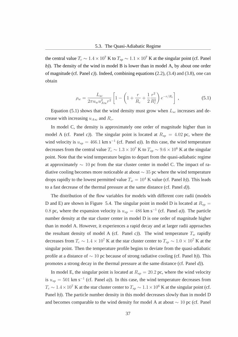
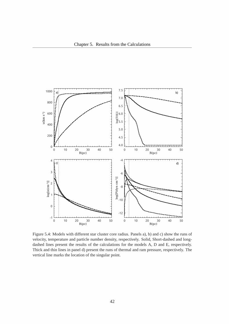
The distribution of the flow variables for models with different core radii (models

D and E) are shown in Figure 5.4. The singular point in model D is located atRsp =

0.8 pc, where the expansion velocity isusp = 486 km s−1 (cf. Panela)). The particle

number density at the star cluster center in model D is one order of magnitude higher

than in model A. However, it experiences a rapid decay and at larger radii approaches

the resultant density of model A (cf. Panelc)). The wind temperatureTw rapidly

decreases fromTc ∼ 1.4 × 107 K at the star cluster center toTsp ∼ 1.0 × 107 K at the

singular point. Then the temperature profile begins to deviate from the quasi-adiabatic

profile at a distance of∼ 10 pc because of strong radiative cooling (cf. Panelb)). This

promotes a strong decay in the thermal pressure at the same distance (cf. Paneld)).

In model E, the singular point is located atRsp = 20.2 pc, where the wind velocity

is usp = 501 km s−1 (cf. Panela)). In this case, the wind temperature decreases from

Tc ∼ 1.4×107 K at the star cluster center toTsp ∼ 1.1×106 K at the singular point (cf.

Panelb)). The particle number density in this model decreases slowly than in model D

and becomes comparable to the wind density for model A at about ∼ 10 pc (cf. Panel

37

Chapter 5. Results from the Calculations

c)).

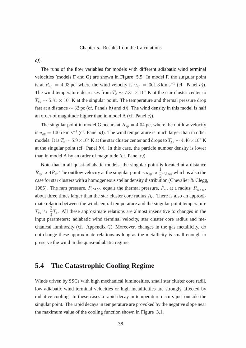
The runs of the flow variables for models with different adiabatic wind terminal

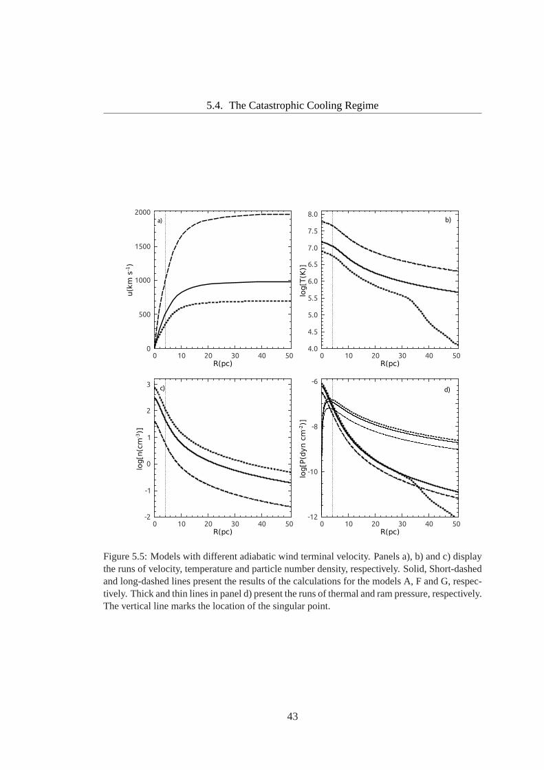
velocities (models F and G) are shown in Figure5.5. In model F, the singular point

is atRsp = 4.03 pc, where the wind velocity isusp = 361.3 km s−1 (cf. Panela)).

The wind temperature decreases fromTc ∼ 7.81 × 106 K at the star cluster center to

Tsp ∼ 5.81 × 106 K at the singular point. The temperature and thermal pressure drop

fast at a distance∼ 32 pc (cf. Panelsb) andd)). The wind density in this model is half

an order of magnitude higher than in model A (cf. Panelc)).

The singular point in model G occurs atRsp = 4.04 pc, where the outflow velocity

is usp = 1005 km s−1 (cf. Panela)). The wind temperature is much larger than in other

models. It isTc ∼ 5.9×107 K at the star cluster center and drops toTsp ∼ 4.46×107 K

at the singular point (cf. Panelb)). In this case, the particle number density is lower

than in model A by an order of magnitude (cf. Panelc)).

Note that in all quasi-adiabatic models, the singular pointis located at a distance

Rsp ≈ 4Rc. The outflow velocity at the singular point isusp ≈1

2uA∞, which is also the

case for star clusters with a homogeneous stellar density distribution (Chevalier & Clegg,

1985). The ram pressure,PRAM , equals the thermal pressure,Pw, at a radius,RRAM

,

about three times larger than the star cluster core radiusRc. There is also an approxi-

mate relation between the wind central temperature and the singular point temperature

Tsp ≈3

4Tc. All these approximate relations are almost insensitive tochanges in the

input parameters: adiabatic wind terminal velocity, star cluster core radius and me-

chanical luminosity (cf. Appendix C). Moreover, changes in the gas metallicity, do

not change these approximate relations as long as the metallicity is small enough to

preserve the wind in the quasi-adiabatic regime.

5.4 The Catastrophic Cooling Regime

Winds driven by SSCs with high mechanical luminosities, small star cluster core radii,

low adiabatic wind terminal velocities or high metallicities are strongly affected by

radiative cooling. In these cases a rapid decay in temperature occurs just outside the

singular point. The rapid decays in temperature are provoked by the negative slope near

the maximum value of the cooling function shown in Figure 3.1.

38

5.4. The Catastrophic Cooling Regime

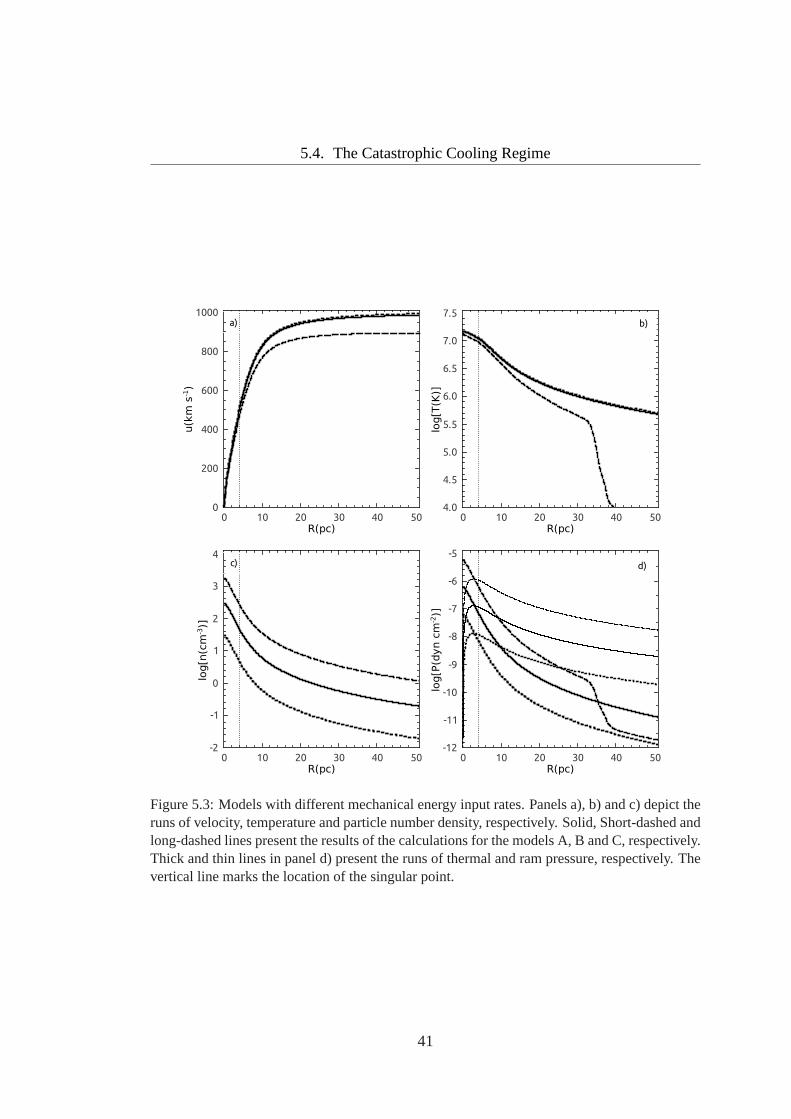
In this regime, the singular point moves rapidly towards thestar cluster center as one

considers more massive clusters, smaller star cluster coreradii and lower adiabatic wind

terminal velocities. The flow outside of the singular point may be thermally unstable.

However, to prove it, it is required to provide 1D or 2D numerical calculations which

is beyond the scope of my thesis.

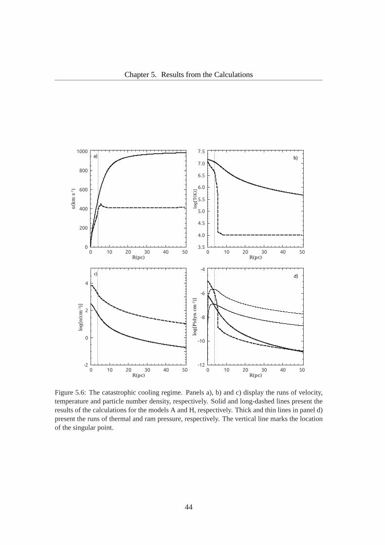
In order to illustrate this regime, I run a model, hereafter model H, with the following

input parameters: an average mechanical luminosityLsc = 7 × 1041 erg s−1, an adia-

batic wind terminal velocityuA∞ = 1000 km s−1, a star cluster core radiusRc = 1 pc

and solar metallicity,Z = Z⊙.

I assumed that the flow is completely ionized at large distances from the star cluster

center and the wind is isothermal when the gas cools down to104 K. This is a realistic

assumption, because the temperature of the gas can be maintained at104 K as long as

the photoionizing flux from the massive stars persists (Tenorio-Tagle et al., 2005).

The hydrodynamic equations in the case of an isothermal winddriven by star clusters

with an exponential stellar density distribution are (cf. AppendixD)

ρw =2qmoR

3

c

uwr2

[

1−

(

1 +r

Rc

+1

2

r2

R2c

)

e−r/Rc

]

, (5.2)

and

duw

dr=

−qmc

2

s

γuw

+2ρwc

2

s

γr− qmuw

ρw

(

uw −c2sγuw

) . (5.3)

Figure 5.6 shows the runs of the flow variables for model H. Thewind velocity

grows fromuw = 0 km s−1 at the star cluster center to its maximum value at∼ 5.5 pc

(cf. Panela)) where the velocity gradient becomes negative due to the rapid fall of

temperature which also causes a strong decay in the thermal pressure (cf. Panelsb) and

d)). Then, at approximately∼ 9 pc, the wind velocity reachesuw ∼ 400 km s−1 and

becomes almost a constant for larger radii.

The singular point for model H is located atRsp = 3.44 pc, where the flow velocity

is usp = 327.4 km s−1. The wind has a central temperature ofTc ∼ 1.2 × 107 K and

39

Chapter 5. Results from the Calculations

goes toTsp ∼ 4.7 × 106 K at the singular point radius. The temperature then rapidly

falls to 104 K at ∼ 8 pc (cf. Panelb)). For larger radii I used the isothermal wind

approximation in order to complete the flow profiles. The winddensity in this model is

one and a half orders of magnitude higher than in model A.

As it has been already discussed in Chapter4, equation (4.19), which defines the

temperature at the singular point, may have two different solutions. In model H there is

only one solution which leads to the temperature at the singular point,Tsp < Tmaxc =

(γ − 1)µionu2

A∞

2γkB, whereTmax

c is the adiabatic wind central temperature (cf. Figure

5.7). Thus in this case one cannot use the solution of equation (4.19) with the higher

temperature as in the quasi-adiabatic wind models. I assumethat the catastrophic cool-

ing regime sets in when the solution with the higher temperature of equation (4.19)

surpasses the valueTmaxc .

Note that in the strong radiative regime, the position of thesingular point is different

from the quasi-adiabatic value.

Finally, in this case none of the approximate relations found for the quasi-adiabatic

wind regime hold and the size of the X-ray envelope is drastically diminished to less

than∼ 5 pc in contrast to the size that one would expect in the quasi-adiabatic cases.

40

5.4. The Catastrophic Cooling Regime

u(km s

-1)

0

200

400

600

800

1000

R(pc)0 10 20 30 40 50

a)

log[n(cm

-3)]

-2

-1

0

1

2

3

4

R(pc)0 10 20 30 40 50

c)

log[T(K)]

4.0

4.5

5.0

5.5

6.0

6.5

7.0

7.5

R(pc)0 10 20 30 40 50

b)

log[P(dyn cm

-2)]

-12

-11

-10

-9

-8

-7

-6

-5

R(pc)0 10 20 30 40 50

d)

Figure 5.3: Models with different mechanical energy input rates. Panelsa), b) and c) depict theruns of velocity, temperature and particle number density, respectively. Solid, Short-dashed andlong-dashed lines present the results of the calculations for the models A, Band C, respectively.Thick and thin lines in panel d) present the runs of thermal and ram pressure, respectively. Thevertical line marks the location of the singular point.

41

Chapter 5. Results from the Calculationsu(km s

-1)

0

200

400

600

800

1000

R(pc)0 10 20 30 40 50

a)

log[T(K)]

4.0

4.5

5.0

5.5

6.0

6.5

7.0

7.5

R(pc)0 10 20 30 40 50

b)

log[P(dyn cm

-2)]

-12

-10

-8

-6

-4

R(pc)0 10 20 30 40 50

d)

log[n(cm

-3)]

-1

0

1

2

3

4

R(pc)0 10 20 30 40 50

c)

Figure 5.4: Models with different star cluster core radius. Panels a), b)and c) show the runs ofvelocity, temperature and particle number density, respectively. Solid, Short-dashed and long-dashed lines present the results of the calculations for the models A, D and E, respectively.Thick and thin lines in panel d) present the runs of thermal and ram pressure, respectively. Thevertical line marks the location of the singular point.

42

5.4. The Catastrophic Cooling Regime

u(km s

-1)

0

500

1000

1500

2000

R(pc)0 10 20 30 40 50

a)

log[T(K)]

4.0

4.5

5.0

5.5

6.0

6.5

7.0

7.5

8.0

R(pc)0 10 20 30 40 50

b)

log[P(dyn cm

-2)]

-12

-10

-8

-6

R(pc)0 10 20 30 40 50

d)

log[n(cm

-3)]

-2

-1

0

1

2

3

R(pc)0 10 20 30 40 50

c)

Figure 5.5: Models with different adiabatic wind terminal velocity. Panels a),b) and c) displaythe runs of velocity, temperature and particle number density, respectively. Solid, Short-dashedand long-dashed lines present the results of the calculations for the modelsA, F and G, respec-tively. Thick and thin lines in panel d) present the runs of thermal and rampressure, respectively.The vertical line marks the location of the singular point.

43

Chapter 5. Results from the Calculationsu(km s

-1)

0

200

400

600

800

1000

R(pc)0 10 20 30 40 50

a)

log[P(dyn cm

-2)]

-12

-10

-8

-6

-4

R(pc)0 10 20 30 40 50

d)

log[n(cm

-3)]

-2

0

2

4

R(pc)0 10 20 30 40 50

c)

log[T(K)]

3.5

4.0

4.5

5.0

5.5

6.0

6.5

7.0

7.5

R(pc)0 10 20 30 40 50

b)

Figure 5.6: The catastrophic cooling regime. Panels a), b) and c) display the runs of velocity,temperature and particle number density, respectively. Solid and long-dashed lines present theresults of the calculations for the models A and H, respectively. Thick and thin lines in panel d)present the runs of thermal and ram pressure, respectively. The vertical line marks the locationof the singular point.

44

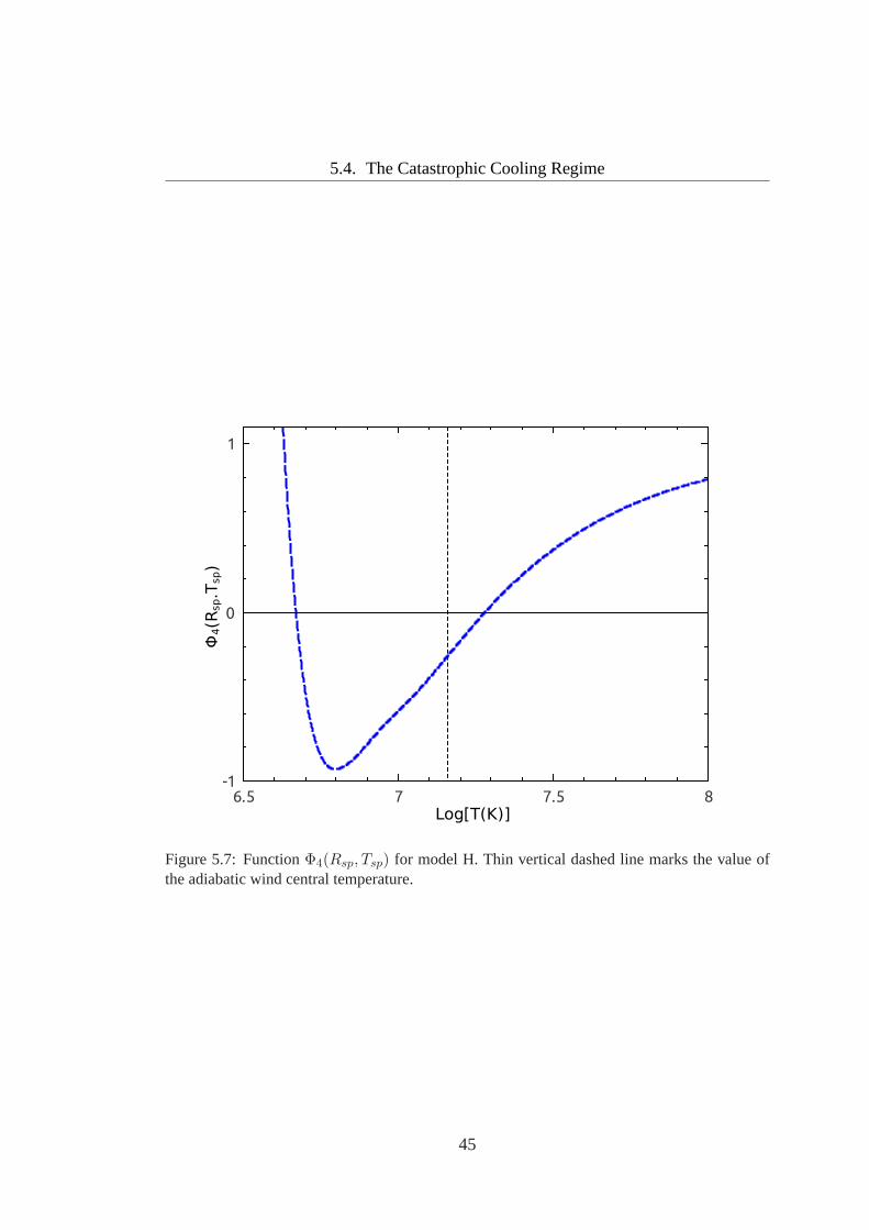
5.4. The Catastrophic Cooling Regime

Φ4(R

sp.T

sp)

-1

0

1

Log[T(K)]6.5 7 7.5 8

Figure 5.7: FunctionΦ4(Rsp, Tsp) for model H. Thin vertical dashed line marks the value ofthe adiabatic wind central temperature.

45

Chapter 6

Concluding Remarks

The aim of this thesis has been to develop a semi-analytic method which allows to study

the hydrodynamics of stationary spherically-symmetric winds driven by young super

star clusters (SSCs) with an exponential stellar density distribution. Considering a non-

homogeneous and more realistic stellar density distribution substantially improves the

hydrodynamic model originally proposed by Chevalier & Clegg (1985). This method

is described in Chapters3 and 4. In contrast with previous works, the method allows

to calculate the position of the singular point self-consistently.

I verified the semi-analytic code by comparing my results with those obtained in the

one-dimensional numeric approach carried out by Ji et al. (2006). Both methods are in

excellent agreement in the quasi-adiabatic regime.

The results from the calculations are presented in Chapter 5.The radial profiles

for the flow variables: expansion velocity, wind temperature, particle number density,

thermal pressure and ram pressure, are presented for a set ofinput parameters.

Two hydrodynamic regimes are discussed

• The quasi-adiabatic regime, in which the singular point is always located at four

times the star cluster core radius. Additionally, the thermal pressure and the ram

pressure are equal at three times the star cluster core radius.

• The catastrophic cooling regime, in which strong radiativecooling moves the

position of the singular point towards the star cluster center. This is different

from the homogeneous case when the singular point is fixed at the star cluster

47

Chapter 6. Concluding Remarks

surface and the stagnation point (Rst; the point where the expansion velocity

is 0 km s−1), moves from the star cluster center towards the star cluster surface

(Tenorio-Tagle et al., 2007).

Radiative cooling leads to the existence of warm (104 K) high velocity (of a few

hundred to a few thousand km s−1) outflows around young star forming regions. This

could be related to the warm isothermal gaseous component found by (Menard et al.,

2009) around star forming galaxies.

I suggest that the catastrophic cooling regime sets in when the solution of equation

(4.19) with the larger temperature at the singular point surpasses the adiabatic wind

central temperatureTmaxc =

(γ − 1)µionu2

A∞

2γkBand the solution with the smaller temper-

ature must be used.

The semi-analytic method presented in this thesis can be easily extended to other

stellar density distributions. In particular, it can be applied to the modified King models

suggested by Elson et al. (1987). It would be also instructive to compare the semi-

analytic results with 1D and 2D numerical simulations and determine whether the flow

outside of the singular point is thermally unstable.

The major results obtained in this thesis are presented in the paper ”The Steady State

Wind Model for Young Stellar Clusters with an Exponential Stellar Density Distribu-

tion” recently accepted for publication in The Astrophysical Journal (astro-ph:1110.0847v1).

48

Appendices

49

Appendix A

The Derivative of the Wind Density

From equation (3.8), the wind density is

ρw =2qmoR

3

cA

uwr2. (A.1)

whereA is a dimensionless term defined as

A =

[

1−

(

1 +r

Rc

+1

2

r2

R2c

)

e−r/Rc

]

. (A.2)

The derivative of the wind velocity can be expressed as

dρwdr

=2qmoR

3

c

uwr2dA

dr+ A

d

dr

(

2qmoR3

c

uwr2

)

, (A.3)

where the derivative of theA is

dA

dr=

1

2

r2e−r/Rc

R3c

. (A.4)

Thus yields

dρwdr

=qmuw

−2qmoR

3

cA

u2wr

2

duw

dr−

4qmoAR3

c

uwr3. (A.5)

51

Appendix A. The Derivative of the Wind Density

Finally, the derivative of the wind density is

dρwdr

=qmuw

−ρwuw

duw

dr−

2ρwr

(A.6)

52

Appendix B

The Derivative of the Local Sound

Speed

The local sound speed is defined as

c2s =γPw

ρw. (B.1)

Applying the chain rule, the derivative of the local sound speed then is

dc2sdr

=γ

ρ2s

(

dPw

drρw −

dρwdr

Pw

)

. (B.2)

According to equation 3.10, the derivative of the thermal pressure is

dPw

dr= −ρwuw

duw

dr− qmuw. (B.3)

Combining B.3 with the derivative of the wind density, derivedin equation A.6, finally

yields

dc2sdr

=duw

dr

[

c2suw

− γuw

]

+qmρw

[

−c2suw

− γuw

]

+2c2sr

. (B.4)

53

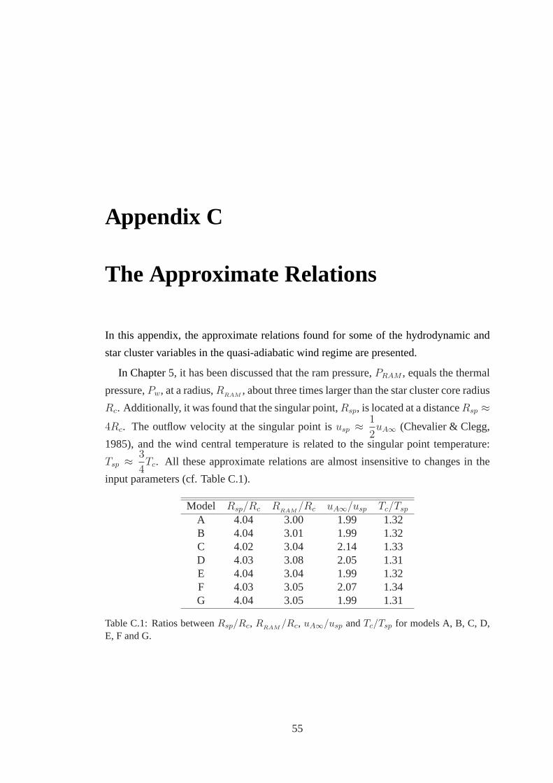
Appendix C

The Approximate Relations

In this appendix, the approximate relations found for some of the hydrodynamic and

star cluster variables in the quasi-adiabatic wind regime are presented.

In Chapter5, it has been discussed that the ram pressure,PRAM , equals the thermal

pressure,Pw, at a radius,RRAM

, about three times larger than the star cluster core radius

Rc. Additionally, it was found that the singular point,Rsp, is located at a distanceRsp ≈

4Rc. The outflow velocity at the singular point isusp ≈1

2uA∞ (Chevalier & Clegg,

1985), and the wind central temperature is related to the singular point temperature:

Tsp ≈3

4Tc. All these approximate relations are almost insensitive tochanges in the

input parameters (cf. Table C.1).

Model Rsp/Rc RRAM

/Rc uA∞/usp Tc/Tsp

A 4.04 3.00 1.99 1.32B 4.04 3.01 1.99 1.32C 4.02 3.04 2.14 1.33D 4.03 3.08 2.05 1.31E 4.04 3.04 1.99 1.32F 4.03 3.05 2.07 1.34G 4.04 3.05 1.99 1.31

Table C.1: Ratios betweenRsp/Rc, RRAM/Rc, uA∞/usp andTc/Tsp for models A, B, C, D,

E, F and G.

55

Appendix D

The Isothermal Wind Hydrodynamic

Equations

The isothermal wind hydrodynamic equations are derived. Since no temperature gra-

dients are considered, the fluid motion is completely definedby only two differential

equations

In the isothermal case, the local sound speed is a constant

c2s =γPw

ρw. (D.1)

Momentum conservation equation (3.2) is

ρwuwduw

dr= −

dPw

dr− qmuw , (D.2)

Since the local sound speed is a constant, the derivative of the thermal pressure can be

calculated analytically from

Pw =ρwc

2

s

γ(D.3)

But in order to minimize changes in the numerical code, one canalso calculate the

thermal pressure from the differential equation

57

Appendix D. The Isothermal Wind Hydrodynamic Equations

dPw

dr=

Pw

ρw

dρwdr

. (D.4)

Using equation (D.4), momentum conservation equation turns into

ρwuwduw

dr= −

Pw

ρw

dρwdr

− qmuw , (D.5)

Combining with equation (A.1), yields

ρwuwduw

dr= −

qmcs2

γuw

+2ρwc

2

s

γr+

ρwc2

s

γuw

duw

dr− qmuw , (D.6)

reordering terms, one can obtain

ρwuwduw

dr

(

uw −c2sγuw

)

= −qmc

2

s

γuw

+2ρwc

2

s

γr− qmuw, (D.7)

and thus yields

duw

dr=

−qmc

2

s

γuw

+2ρwc

2

s

γr− qmuw

ρw

(

uw −c2sγuw

) . (D.8)

58

Figure Index

1.1 HST image of NGC 1569 . . . . . . . . . . . . . . . . . . . . . . . . .2

1.2 HST image of the star cluster R136 . . . . . . . . . . . . . . . . . . . . 3

2.1 Schematic representation of the model . . . . . . . . . . . . . . .. . . 10

2.2 The adiabatic sound speedversusthe escape velocity . . . . . . . . . . 12

2.3 A modified Kingversusthe exponential profile . . . . . . . . . . . . . 14

3.1 The Cooling Function for solar metallicity . . . . . . . . . . . .. . . . 19

4.1 The Solution Topology . . . . . . . . . . . . . . . . . . . . . . . . . . 22

4.2 FunctionΦ4(Rsp, Tsp) for differentLsc andRsp . . . . . . . . . . . . . 27

4.3 Tsp versusRsp . . . . . . . . . . . . . . . . . . . . . . . . . . . . . . . 29

4.4 The Radial Derivative of the Wind Velocity . . . . . . . . . . . . .. . 32

5.1 Comparison with the results of Ji et al. (2006) . . . . . . . . . .. . . . 34

5.2 The reference model . . . . . . . . . . . . . . . . . . . . . . . . . . . 35

5.3 Models with different mechanical energy input rates . . .. . . . . . . . 41

5.4 Models with different star cluster core radius . . . . . . . .. . . . . . 42

5.5 Models with different adiabatic wind terminal velocity. . . . . . . . . 43

5.6 The catastrophic cooling regime . . . . . . . . . . . . . . . . . . . .. 44

5.7 FunctionΦ4(Rsp, Tsp) for model H . . . . . . . . . . . . . . . . . . . . 45

59

Table Index

5.1 The Input Parameters . . . . . . . . . . . . . . . . . . . . . . . . . . .36

C.1 The Approximate Relations . . . . . . . . . . . . . . . . . . . . . . . . 55

61

References

Arp, H., & Sandage, A. 1985, AJ, 90, 1163

Billett, O. H., Hunter, D. A., & Elmegreen, B. G. 2001, in Bulletin of the AmericanAstronomical Society, Vol. 33, American Astronomical Society Meeting Abstracts,1329–+

Canto, J., Raga, A. C., & Rodrıguez, L. F. 2000, ApJ, 536, 896

Chevalier, R. A., & Clegg, A. W. 1985, ApJ, 317, 44

Clarke, C. J., & Carswell, R. F. 2007, Principles of Astrophysical Fluid Dynamics(Cambridge University Press)

Elson, R. A. W., Fall, S. M., & Freeman, K. C. 1987, ApJ, 323, 54

Heckman, T. M., Armus, L., & Miley, G. K. 1990, ApJS, 74, 833

Holtzman, J. A., Faber, S. M., Shaya, E. J., Lauer, T. R., Groth, J., Hunter, D. A.,Baum, W. A., Ewald, S. P., Hester, J. J., Light, R. M., Lynds, C. R.,O’Neil, Jr., E. J.,& Westphal, J. A. 1992, AJ, 103, 691

Ji, L., Wang, Q. D., & Kwan, J. 2006, MNRAS, 372, 497

Johnson, H. E., & Axford, W. I. 1971, ApJ, 165, 381

Johnson, K. E., Leitherer, C., Vacca, W. D., & Conti, P. S. 2000,AJ, 120, 1273

King, I. 1962, AJ, 67, 471

Lada, C. J., & Lada, E. A. 2003, ARA&A, 41, 57

Lamers, H. J. G. L. M., & Cassinelli, J. 2007, Introduction to Stellar Winds (CambridgeUniversity Press)

Larsen, S. S., Brodie, J. P., & Hunter, D. A. 2004, AJ, 128, 2295

Leitherer, C., Schaerer, D., Goldader, J. D., Gonzalez Delgado, R. M., Robert, C.,Kune, D. F., de Mello, D. F., Devost, D., & Heckman, T. M. 1999,ApJS, 123, 3

63

References

Mayya, Y. D., Romano, R., Rodrıguez-Merino, L. H., Luna, A., Carrasco, L., & Rosa-Gonzalez, D. 2008, ApJ, 679, 404

McCrady, N., Gilbert, A. M., & Graham, J. R. 2003, ApJ, 596, 240

Melnick, J., Moles, M., & Terlevich, R. 1985, A&A, 149, L24

Melo, V. P., Munoz-Tunon, C., Maız-Apellaniz, J., & Tenorio-Tagle, G. 2005, ApJ,619, 270

Menard, B., Wild, V., Nestor, D., Quider, A., & Zibetti, S. 2009, ArXiv e-prints

Mengel, S., Lehnert, M. D., Thatte, N., & Genzel, R. 2002, A&A,383, 137

Meurer, G. R., Heckman, T. M., Leitherer, C., Kinney, A., Robert, C., & Garnett, D. R.1995, AJ, 110, 2665

O’Connell, R. W., Gallagher, III, J. S., & Hunter, D. A. 1994, ApJ, 433, 65

Portegies Zwart, S. F., McMillan, S. L. W., & Gieles, M. 2010,ARA&A, 48, 431

Raga, A. C., Velazquez, P. F., Canto, J., Masciadri, E., & Rodrıguez, L. F. 2001, MN-RAS, 559, L33

Raymond, J. C., Cox, D. P., & Smith, B. W. 1976, ApJ, 204, 290

Rockefeller, G., Fryer, C. L., Melia, F., & Wang, Q. D. 2005, ApJ, 623, 171

Rodrıguez-Gonzalez, A., Canto, J., Esquivel, A., Raga, A. C., & Velazquez, P. F. 2007,MNRAS, 380, 1198

Sarazin, C. L., & White, III, R. E. 1987, ApJ, 320, 32

Silich, S., Tenorio-Tagle, G., & Munoz-Tunon, C. 2003, ApJ, 590, 791

Silich, S., Tenorio-Tagle, G., & Munoz-Tunon, C. 2007, ApJ, 669, 952

Silich, S., Tenorio-Tagle, G., & Rodrıguez-Gonzalez, A. 2004, ApJ, 610, 227

Tenorio-Tagle, G., Silich, S., Rodrıguez-Gonzalez, A., & Munoz-Tunon, C. 2005, ApJ,620, 217

Tenorio-Tagle, G., Wunsch, R., Silich, S., & Palous, J. 2007, ApJ, 658, 1196

Weigelt, G., & Baier, G. 1985, A&A, 150, L18

Whitmore, B. C. 2000, ArXiv Astrophysics e-prints

Whitmore, B. C., & Schweizer, F. 1995, AJ, 109, 960

64

References

Whitmore, B. C., Zhang, Q., Leitherer, C., Fall, S. M., Schweizer, F., & Miller, B. W.1999, AJ, 118, 1551

Wunsch, R., Silich, S., Palous, J., Tenorio-Tagle, G., & Munoz-Tunon, C. 2011, ApJ,740, 75

Wunsch, R., Tenorio-Tagle, G., Palous, J., & Silich, S. 2008, ApJ, 683, 683

65