The Impact of the Great Recession on Emerging Markets

Ricardo Llaudes, Ferhan Salman, and Mali Chivakul

WP/10/237

© 2010 International Monetary Fund WP/10/237

IMF Working Paper

Strategy, Policy and Review Department

The Impact of the Great Recession on Emerging Markets

Prepared by Ricardo Llaudes, Ferhan Salman, and Mali Chivakul

Authorized for distribution by Lorenzo Giorgianni

October 2010

Abstract

This Working Paper should not be reported as representing the views of the IMF. The views expressed in this Working Paper are those of the author(s) and do not necessarily represent those of the IMF or IMF policy. Working Papers describe research in progress by the author(s) and are published to elicit comments and to further debate. This paper examines the impact of the recent global crisis on emerging market economies (EMs). Our cross-country analysis shows that the impact of the crisis was more pronounced in those EMs that had initial weaker fundamentals and greater financial and trade linkages. This effect is observed along a number of dimensions, such as growth, stock market performance, sovereign spreads, and credit growth. This paper also shows that during this crisis, pre-crisis reserve holdings helped to mitigate the initial growth collapse. This finding contrasts with other studies that fail to find a significant relationship between reserves and the growth decline. This paper argues that our preferred measure of impact is a more accurate reflection of the true impact of the crisis on EMs.

JEL Classification Numbers: F01, G01, F15, F42

Keywords: Emerging markets, global crisis, vulnerabilities, reserves, linkages

Author’s E-Mail Address: rllaudes@imf.org, fsalman@imf.org, mchivakul@imf.org

2

Contents Page

 I. Introduction ............................................................................................................................3 II. A Broad View of the Impact of the Crisis .............................................................................5 III. Econometric Analysis ........................................................................................................11 A. Measuring impact: Alternative metrics………………………………………........11 B. Impact on growth………………………………………………………………… 13 C. The role of reserves………….…………………………………………………….15 D. Impact on sovereign spreads………………………………………………………18 E. Impact on credit……………………………………………………………………19 F. Further issues………………………………………………………………………22 IV. Conclusions........................................................................................................................24 References………...………………………………………………………………………….25 Box 1. Assessments of Underlying Vulnerabilities in Emerging Market Countries ...............27 Tables

1a. Impact of the crisis 5 1b. Correlations - Real and financial variables 7 2a. Regressions for percent change in real output between peak and trough (growth_3) 14 2b. Regressions for percent change in real output between peak and trough (growth_4) 14 3. Dependent variable: Real output peak to trough (growth_3) 17 4. Determinants of the change in spreads from trough to peak (in percent) 19 5. Determinants of peak-to-trough real credit growth 20 Figures

1. Pre-crisis external vulnerabilities 4 2. Median stock market indices 8 3. Capital flows to emerging markets 9 4. Impact of the crisis on output 10 5. Financial and corporate vulnerabilities 11 6. Alternative growth metrics 12 7. Reserve coverage and output collapse 15 8. Initial reserves and reserve use 17 9. Fall in reserves (peak to trough, percent of 2008 GDP) 18 10. Credit developments 21 11. Deleveraging 21 12. Banks' probability of default 22 13. Impact of crisis: Country variability in outcomes 23 Appendix 1. Country sample ...................................................................................................28 Appendix 2. List of variables 29 Appendix 3. Reserve Robustness with Alternative Control Variables 30

3

I. INTRODUCTION1

The global economy is by now emerging from the largest shock in the post-war era. Following years characterized by strong global growth and increasing trade and financial linkages, the implosion in advanced economy financial centers, especially after the collapse of Lehman in September 2008, quickly spilled over to emerging market economies (EMs). As a result, growth of the global economy fell by 6 percentage points from its pre-crisis peak to its trough in 2009, the largest straight fall in global growth in the post-war era. Similarly, real output in EMs fell about 4 percent between 2008Q3 and 2009Q1, the most intense period of the crisis. However, this average performance masked considerable variation across EMs. Ranking EMs by output impact, those in the worst affected quartile—mostly in emerging Europe—experienced a 11 percent real output contraction during the period while those EMs in the least affected quartile saw their output grow by 1 percent.

Against this backdrop, this paper explores the channels and factors that shaped the initial impact of the crisis on emerging market economies with a view to explaining the observed heterogeneous experience across EMs. Using a sample of around 50 emerging market economies, the impact of the crisis is measured along several dimensions, including the actual decline in quarterly growth, the decline in stock markets, the rise in sovereign spreads, and the decline in credit growth. To account for initial conditions and pre-crisis fundamentals, this paper uses a unique measure of vulnerabilities developed by IMF staff that, by virtue of its construction, allows for a consistent comparison of vulnerabilities across EMs. Given that for most EMs this was an externally driven crisis, this paper focuses on external sector vulnerabilities prior to the crisis, including current account deficits, reserve holdings, and external debt levels among others.

The paper’s primary findings are twofold: (i) as expected, countries that were more open to trade and financial linkages were more affected by the crisis and (ii) countries that had improved policy fundamentals and reduced vulnerabilities in the pre-crisis period reaped the benefits of these reforms during the crisis. In other words, controlling for other determinants of impact such as trade and financial openness, countries that had better pre-crisis fundamentals and vulnerability indicators experienced less severe output contractions and widening of sovereign spreads. Furthermore, higher international reserves holdings, by reducing external vulnerability, helped buffer the impact of the crisis. But reserves had diminishing returns: at very high levels of reserves there is little discernable evidence of their moderating impact on output collapse.

1 We would like to thank Reza Baqir, Lorenzo Giorgianni, Gavin Gray, Aasim Husain, Manrique Saenz, Bikas Joshi for helpful contributions and Petya Kehayova, Apinait Amranand and Gabriel Presciuttini for excellent research assistance. Comments from seminar participants and departments within the IMF and the World Bank are appreciated. This paper expands on ideas presented in IMF (2010), “How did Emerging Markets Cope in the Crisis?” It also benefits from consultations with authorities in Russia, Indonesia, and the Philippines.

4

To our knowledge, this is the first paper that finds a significant and robust relationship, a non-linear one, between EMs’ reserve holdings and the actual decline in growth experienced during the crisis. This could owe to the fact that our preferred measure of impact, estimated as the country-specific peak-to-trough decline in quarterly real GDP, is a more accurate measure of impact that those used in related papers (Berkmen and others (2009), Lane and Milesi-Ferretti (2010), and Blanchard and others. (2010)). These studies either use annual data, which do not give any indication of important intra-annual variations in growth, or assume that growth peaks and troughs across EMs took place in the same quarter. As it will be shown, countries entered and exited the crisis at very different points in time. Another contribution of this paper to the literature is the systematic analysis of the impact of the crisis on financial variables such as sovereign spreads and credit growth.

The role played by pre-crisis vulnerabilities has important implications for policy makers. During the thick of the crisis around the time of Lehman Brothers’ bankruptcy, EM asset prices fell across the board. At the time it was not clear whether EMs that had invested in improving fundamentals in the preceding years would fare any better than others. The main message from this paper is that markets do discriminate across EMs and prior progress was rewarded. Countries that entered the crisis with lower vulnerabilities had worked to reduce them in the preceding period Figure 1. This message also highlights the need for EMs emerging from the crisis with high vulnerabilities to protect themselves against future shocks.

This paper contributes to and enhances the body of literature assessing the impact of the crisis on EMs. In a comparable analysis, Berkmen and others (2009) use a similar sample of EMs but their measure of impact looks at “revisions of projections for GDP growth in 2009, comparing forecasts prior to and after the intensification of the crisis in September 2008.” This is not an optimal measure of impact as growth forecasts could be subject to the

-0.2

0.0

0.2

0.4

0.6

0.8

1.0

1.2

-0.8 -0.6 -0.4 -0.2 0 0.2 0.4 0.6

Ext

ern

al v

uln

era

bili

ty in

de

x (2

00

7)

Figure 1. Pre-crisis External Vulnerabilities 1/

1/ Lower numbers indicate lower vulnerabilitySource: Vulnerability Exercise, Spring 2007

Change in external vulnerability index (2003-07)

5

forecaster’s bias and, moreover, forecasters may change across vintages. Exploring the impact of the crisis on growth, consumption, and domestic demand, Lane and Milesi-Ferretti (2010) find no evidence that greater financial integration amplified the impact of the crisis while Berglöf and others (2009) only find mixed evidence. Results in these two studies may be affected by the choice of countries in their sample, as the former combines advanced economies with emerging markets and low income countries while the latter focuses on Emerging Europe. On the other hand, analysis by the BIS (2009a, 2009b) suggests that financial connectedness did indeed matter. Rose and Spiegel (2009a, 2009b) fail to find any link between the behavior of the most widely-used determinants of crises and the incidence of the crisis across countries. However, the sample used is restricted to declines in growth through 2008, a sample cut too short to capture the full impact of the crisis.

II. A BROAD VIEW OF THE IMPACT OF THE CRISIS

While the global crisis started in financial centers in the advanced economies (AEs), it took a heavy toll on EMs: the median EM suffered a somewhat larger decline in output than the median AE, 4.9 percent for the former against 4.5 percent for the latter, measured from the pre-crisis peak to the trough during the crisis (see Table 1a). Moreover, the impact was more varied in EMs, with several EMs affected more than the worst-hit AEs while some other EMs continued to grow through the crisis period. High frequency financial variables exhibit similar behavior. While on average EMs experienced as large a decline in stock markets and a widening of sovereign spreads as AEs, there was considerably greater cross-country variability in EMs. The next sections in this paper will use regression analysis to shed some light on the factors and country characteristics determining these differing outcomes.

Output collapse 1/Median -4.9 -4.525th percentile -8.4 -6.675th percentile -2.0 -2.9

Stock market collapse 1/Median -57.1 -55.425th percentile -72.0 -64.175th percentile -45.2 -49.0

Rise in sovereign spreads 2/Median 462 46525th percentile 287 …75th percentile 772 …

Source: Haver; Bloomberg; Fund staff calculations.

Emerging Markets

Advanced Economies

1/ Measured as percent change from peak to trough. 2/ Measured as increase in basis points from trough to peak. For AEs, table reports rise in spreads on US corporates rated BBB.

Table 1a. Impact of the Crisis

6

A convenient way to approach the analysis of the impact of the crisis is to classify EMs on the basis of their pre-crisis vulnerabilities. Pre-crisis vulnerabilities can be measured in different ways.2 However, measuring vulnerabilities consistently across countries and over time can be a challenging task. IMF staff has developed a methodology for this purpose as part of the internal semi-annual vulnerability exercise for emerging market economies (VEE; see Box 1).3 Given that for most EMs this was an externally driven crisis, this paper primarily uses the indicator-based external vulnerability index from the spring 2007 round of the VEE, the last exercise before the onset of market volatility in late 2007. The terms “low,” “medium,” and “high” vulnerability as used in the rest of the paper pertain to the ratings on this vulnerability index in the spring 2007 round of the VEE. It is worth noting that of the “high” vulnerability group, about half the countries was located in Emerging Europe. The country sample used in the paper is provided in Appendix 1.

The impact of the crisis can be measured along several dimensions:

Impact on the real economy. As will be further elaborated in the next section, the preferred measure of real impact in this paper is the percent change in seasonally adjusted quarterly GDP from each country’s peak to its respective trough during the crisis. 4

Impact on financial markets and the banking sector. This is measured, for each country, by the (a) change in the average monthly stock market index during the crisis; (b) collapse in real private sector credit growth from its peak to trough and the difference between pre- and post-crisis average monthly credit flows in percent of GDP; and (c) rise in the average monthly EMBI sovereign spread from its trough to peak (in basis points). Similar to the output loss analysis, country variation in peaks and troughs is taken into account.

These measures of impact tend to provide a consistent story. Table 1b shows simple correlation coefficient between the peak to trough percentage change in real GDP, credit growth, spreads and stock markets. The result suggest that those EMs that fell more in financial terms also fell more in real terms, which was also accompanied by a credit collapse.

2 The terms “vulnerabilities” and “fundamentals” are used interchangeably in this paper. Box 1 describes the specific metrics used to measure vulnerabilities.

3 The VEE was established in 2001 to inform staff’s surveillance of emerging market countries. It examines several indicators against thresholds in the public, external, financial, and corporate sectors, to classify a country as having a “low,” “medium,” or “high” underlying vulnerability in each sector and overall. For confidentiality reasons it is not published. Box 1 provides more details.

4 An alternative measure of impact could be the change in output between 2008Q3 and 2009Q1, the peak and trough, respectively, for the typical EM. However, there is considerable country level variation in peaks and troughs and using this approach would have been accurate for only around one half of the EMs in the sample.

7

Notably, both credit and growth are correlated with spreads and stocks (with expected signs). A somewhat surprising result is that changes in stock markets do not appear to be correlated with changes in spreads. This could owe to the fact that markets differentiated between stresses in the sovereign and stresses in the corporate sector. For example, an EM that has a strong fiscal position may not experience a rise in spreads although the stock market could take a hit as exporting companies’ earnings prospect falls. China, for example, only saw a 84 bps rise in spreads (in the best performing quartile) but its stock market fell by 67 percent (median fall is 57 percent).

Turning now to developments in financial markets, a pattern of re-coupling leading to re-decoupling emerges in the financial transmission of the crisis. This finding lends some support to arguments made in the years prior to the crisis over the possibility that some EMs had “decoupled” from AEs. That is, EMs were no longer dependent on AEs demand to sustain robust rates of growth. To further assess financial developments across EMs in relation to AEs and how investors differentiated between countries, Figure 2 traces daily stock market indices across AEs and EMs by their level of vulnerability in spring 2007. Similar to several other studies, the start of the crisis is taken to be August 9, 2007 when three funds that had invested in subprime mortgages were suspended from trading and the Fed, ECB, and BoJ undertook coordinated liquidity injection. 5 Three phases of transmission emerge:

Decoupling. First, some EMs seemed to decouple from AEs between the start of the crisis and collapse of Lehman. Until a few weeks before Lehman’s bankruptcy announcement, stock markets in low and medium pre-crisis vulnerability EMs were 15 percent below their levels of August 2007, while those in AEs and high vulnerability EMs had already fallen around 30 percent.

5 See Cecchetti (2008) and Taylor and Williams (2008).

Growth Stocks Spreads1/ Credit growth

Growth 1.00

Stocks 0.39 1.00

Spreads -0.24 -0.03 1.00

Credit growth 0.41 0.42 -0.29 1.00

(peak-to-trough change, percent)

Table 1b. Correlations - Real and Financial Variables

1/ Measured as change from trough to peak.

8

Re-coupling. This differentiation across emerging markets came to an end in the second phase as Lehman’s collapse triggered panic in the global economic landscape and all EMs fell almost uniformly.

Re-decoupling. With the return of stability in the third phase of transmission, EMs re-decoupled and a striking gap opened between high vulnerability countries and others. Overall, since August 2007, while stock markets in low and medium vulnerability countries have broadly recovered to pre-crisis levels, those in countries with high vulnerabilities on the eve of the crisis remain depressed. This pattern of market discrimination has continued during the recent sovereign crisis in Europe’s periphery: during the April-May period of highest turbulence, stock markets declined by around 7 percent in the low and medium vulnerability economies, by around 13 percent in the high vulnerability ones, and by around 17 percent in AEs.

The pattern in the fall in the stock market indices is also reflected in the capital flows data. Figure 3 shows that gross portfolio flows fell in the last quarter of 2008 for all EMs and in spite of their vulnerability ratings. However, starting from the first quarter of 2009, EMs with low and medium vulnerabilities already started to see positive portfolio flows while those with high vulnerabilities still experienced gross outflows. Experience across regions is also striking. Emerging Europe, home to many EMs with high vulnerabilities, did not see portfolio flows coming back until 2009Q2, while in other regions such as Asia, portfolio flows never did experience much of a decline.

0

20

40

60

80

100

120

Jan-07 Apr-07 Jul-07 Oct-07 Jan-08 Apr-08 Jul-08 Oct-08 Jan-09 Apr-09 Jul-09 Oct-09 Jan-10 Apr-10 Jul-10

EM Low & Medium Vulnerability

AM

EM High Vulnerability

Figure 2.Median Stock Market Indices(August 9, 2007 = 100, medians)

Start of crisis,August 9, 2007

Lehman Brothers

G20 Summit - London

Fedrateat zero

IMFReform Lending Facilities

Source: Bloomberg; Fund staff calculations.

EFSF Announcement

9

Figure 3. Capital flows to Emerging Markets

As regards the macroeconomic impact, countries that experienced a decline in vulnerabilities before the crisis came out well ahead of others and experienced shallower downturns. This is illustrated in both the timing of experiencing a fall in output and the magnitude of the decline:

Timing of collapse in real activity. By the third quarter of 2008, the majority of countries that had high or medium pre-crisis vulnerabilities were contracting (Figure 4; left panel). In contrast, low pre-crisis vulnerability EMs held out longer before succumbing to global headwinds. Even through the worst of the crisis in 2009Q1, many low vulnerability countries did not experience a fall in output. Similarly, in the recovery phase, economies with low and medium pre-crisis vulnerabilities have tended to return to positive quarterly growth much sooner than those with high vulnerabilities.

Magnitude of collapse in real activity. A similar message emerges from a comparison of the magnitude of the fall in real GDP (Figure 4; right panel). Countries with low and medium vulnerabilities suffered much smaller real output collapses and are experiencing much steeper recoveries than other EMs. These countries also contracted much less than AEs.

Source: Haver and IMF.

-50

0

50

100

150

200

250

300

350

400

450

2006Q1 2007Q1 2008Q1 2009Q1 2010Q1

Gross Capital Flows Excluding FDI to Asian EMs(In USD billion)

Other LiabsPortolio EquityPortfolio debt

-50

0

50

100

2006Q1 2007Q1 2008Q1 2009Q1 2010Q1

Gross Capital Flows Excluding FDI to Latin American EMs(In USD billion)

Other Liabs

Portolio Equity

Portfolio debt

-50

0

50

100

150

2006Q1 2007Q1 2008Q1 2009Q1 2010Q1

Gross Capital Flows Excluding FDI to European EMs (In USD billion)

Other Liabs

Portolio Equity

Portfolio debt

-100

-50

0

50

100

150

2005Q1 2006Q1 2007Q1 2008Q1 2009Q1 2010Q1

Gross Portfolio Flows by External Vulnerability Rating in Spring 2007, (in USD billion)

M&L

H

10

An interesting and perhaps surprising result emerging from the analysis above is that highly vulnerable EMs experienced a smaller initial fall in output during this crisis than EMs in past crises.6 The global coordinated response to this crisis and the provision of quick and large amounts of financing from international institutions, including the IMF, allowed countries to smooth adjustment. In addition, past EM crises often involved banking crises, which was not the case this time round. This was partly due to the crisis having emerged in AE financial centers, but also probably owed to the general absence of currency crises that could have severely impaired banks and corporate balance sheets. Moreover, many EMs entered this crisis on the back of improvements in financial and corporate sectors vulnerability indicators (Figure 5). An exception is the average trend for European EMs, where financial sector vulnerabilities did not improve during 2000−07, unlike in other regions where there was a substantial improvement.

On the other hand, for countries with weak fundamentals, this crisis may turn out to be more protracted than past crisis, which tended to exhibit more of a U-shaped recovery. This result is line with the IMF (2009a and 2009b) finding that recessions after financial crisis are unusually long, particularly in the context of a global downturn.

6 Past capital account crisis cases—for comparison purposes—are Mexico (1994), Indonesia (1997), Korea (1997), Malaysia (1997), Philippines (1997), Thailand (1997), Brazil (1998), Colombia (1998), Ecuador (1998), Russia (1998), Turkey (2000), Argentina (2001), and Uruguay (2001). Dates in parentheses are those of crisis inception. Comparisons with past crises should be interpreted with caution, owing to differing external circumstances prevailing during different episodes. Ramakrishnan and Zalduendo (2006) and Reinhart and Rogoff (2008) use similar country samples of past crises.

Figure 4. Impact of Crisis on Output

0

10

20

30

40

50

60

70

80

90

100

2007Q4 2008Q1 2008Q2 2008Q3 2008Q4 2009Q1 2009Q2 2009Q3 2009q4

Per

cent

of

VE

cat

ego

ry

Proportion of Countries with Negative Quarterly Growth by Level of External Vulnerability

High vulnerability Medium vulnerability Low vulnerability

Source: VEE Spring 2007; Haver; National authorities; Fund staf f calculations

90

92

94

96

98

100

102

104

106

2008Q2 2008Q3 2008Q4 2009Q1 2009Q2 2009Q3 2009Q4 2010Q1

Real GDP(2008q2 = 100, seasonally adjusted, medians)

EM AEEM: Low & Medium Vulnerability EM: High VulnerabilityPast crises

11

III. ECONOMETRIC ANALYSIS

A. Measuring impact: Alternative metrics

The analysis in this paper was undertaken using four alternative measures of output loss to better assess the robustness of the findings to the choice of impact measure:

A simple gauge is how far output fell in the two quarters after the collapse of Lehman Brothers, measured by the percentage change in seasonally adjusted real GDP between 2008Q3 and 2009Q1. In this paper, we refer to this measure as “Growth 1,” similar to that used by Lane and Milesi-Ferretti (2010) in that it applies equal timing to all countries in the sample.

A drawback of Growth 1 is that it does not take into account growth dynamics prior to the crisis and where output might have been in the absence of a crisis. To gauge output loss in that (counterfactual) sense, a second growth measure (“Growth 2”) is calculated as the log difference between actual seasonally adjusted real GDP in 2009Q1 and a counterfactual projection for real GDP in 2009Q1 based on a linear trend estimated over 2003-2007. This approach is similar in spirit to that used by Abiad and others (2010) to evaluate medium-term output dynamics following banking crises.

The above two measures implicitly assume each EM’s output peaked in 2008Q3 and troughed in 2009Q1. However, as already shown, there is considerable heterogeneity in the timing of the crisis across countries. Indeed, this timing would only be accurate for about half the sample. Therefore, a third measure was devised (“Growth 3”),

Figure 5. Financial and Corporate Vulnerabilities

Source: VEE Fall 2009 (lower values of the index indicate lower vulnerability).

0.0

0.1

0.2

0.3

0.4

0.5

0.6

0.7

2000 2002 2004 2006 2008

EuropeLatin America

Asia

Middle East

Financial Sector Vulnerability Index (Index range: 0 - 1)

0.0

0.1

0.2

0.3

0.4

0.5

0.6

0.7

0.8

0.9

1997 1999 2001 2003 2005 2007

Corporate Sector Vulnerability Index (Index range: 0 - 1)

Europe

Latin America

Asia

12

which is the country-specific peak to trough percent change in quarterly seasonally adjusted real GDP. This measure of impact is unique to our study.

Finally, a fourth measure (“Growth 4”) was calculated that takes into account cross-country heterogeneity in both the counterfactual growth path and the timing of recovery. It was defined as the log difference between actual seasonally adjusted real GDP at the country’s trough, and projected real GDP based on a linear trend estimated over 2003−07.

The preferred measure in this paper is “growth 3,” based on the actual change in output and each country’s peak and trough. This is a more accurate and an easier to interpret measure of impact. Moreover, one shortcoming of using “growth 4” is that it may overestimate the impact of the crisis. In some countries growth in 2003-07 was unsustainably high and would have slowed down even without the crisis. As depicted in Figure 6, “growth 3” is highly correlated with “growth 1” and “growth 4,” though the correlation is stronger with “growth 4” (right panel) as can be seen from the tighter alignment of the scatter plot along the 45 degree line. While the results are robust to using either of these measures the analysis below will focus on the last two. Analogous to “growth 3,” country-specific peak to trough changes were also estimated for EMBI spreads and for credit growth.

Figure 6. Alternative growth metrics

-.2

-.15

-.1

-.05

0.0

5

Rea

l GD

P g

row

th, 2

008

Q3

to 2

009

Q1

-.25 -.2 -.15 -.1 -.05 0

Real GDP growth, peak to trough

Source: Haver, WEO, and Staff estimates

Country specific variation in output peaks and troughsMeasuring Output Loss: 1

-.4

-.3

-.2

-.1

0

Dev

iatio

n fr

om

tren

d gr

ow

th p

rior

to 2

008

-.25 -.2 -.15 -.1 -.05 0Real GDP growth, peak to trough

Source: Haver, WEO, and Staff estimates

Role of counterfactualMeasuring Output Loss: 2

13

B. Impact on growth

This section assesses the impact of pre-crisis external vulnerabilities on output collapse, controlling for global linkages. The primary regression specification used in this paper explains the fall in real output as a function of (a) pre-crisis vulnerabilities; (b) trade connectedness with the rest of the world; and (c) international financial integration. After trying several alternative measures for each of these three categories, the following three measures best explained the cross-country variation of impact: (a) the external vulnerability index in the Spring 2007 round of the VEE; (b) the percent change in domestic demand of AE trading partners weighted by trade shares and computed over a similar period to the peak-to-trough change in each EM’s output; and (c) the consolidated stock of claims of BIS reporting banks (immediate borrower basis) on EMs in percent of the EM’s GDP in December 2007. A number of other indicators, including regional dummies and type of exchange rate regime, were tried as part of the empirical analysis, either as alternatives for the above three or as additional controls, but they did not affect the central findings (Table in Appendix 2).

The least vulnerable EMs, on average, contracted 6½ percentage points less than the most vulnerable EMs (Table 2a). All four factors that influence the external vulnerability index were also individually significant, with the exception of external debt in percent of exports (Table 2a, columns 2–5).7 More externally vulnerable EMs, in particular those with high current account deficits, may have experienced sharper declines in domestic demand, contributing to the decline in output. In many instances, countries with high external vulnerabilities were the countries with pre-crisis domestic demand booms fueled by capital-inflows, which ended when the capital inflows suddenly stopped.8 Other standard sectoral vulnerability indicators—fiscal, financial, corporate—do not stand out as significant factors in explaining the output decline.

Trade linkages were another important determinant of output collapse. Coefficients from the first regression in Table 2a indicate that EMs experienced an additional 1½ percentage point reduction in real output during the crisis for every percentage point fall in domestic demand in their advanced economy trading partners. Large EMs, for who exports formed a smaller component of their aggregate demand (such as Indonesia and India), consequently experienced smaller real shocks. As has been documented elsewhere, trade fell more in this crisis than in past global recessions, in part a reflection of increasing interconnectedness and the responsiveness of global supply chains (Freund, 2009). Nevertheless, contrary to early concerns, problems with trade finance were not a principal cause of the sharp collapse in

7 As noted in Box 1, these four factors cannot be added simultaneously to the regression due to collinearity.

8 Bakker and Gulde (2010) for example shows that the decline in domestic demand was most pronounced in the countries that had built up the largest imbalances during the boom years for emerging European countries.

14

trade. Also, even though trade dispute filings intensified during the crisis, a wholesale rise in protectionism did not materialize.

To check the robustness of the results to the choice of impact measure, Table 2b replicates the regression specifications in Table 2a but replacing “growth 3” with “growth 4” as dependent variable. The results are consistent with those previously obtained for all specifications. Indeed, the results appear to be stronger, with somewhat higher R-squared values. The least vulnerable EMs, on average, now contracts 7½ percentage points less than the most vulnerable EMs.

Sample All EMs All EMs All EMs All EMs All EMs

External sector vulnerability index (ranged 0 - 1) -6.40 **(3.04)

Domestic demand growth in AE trading partners (percent) 1.44 ** 1.47 ** 1.68 *** 1.63 *** 1.53 **(0.68) (0.63) (0.53) (0.59) (0.65)

Foreign bank claims (percent of GDP, expressed in logs) -1.7 * -1.94 ** -1.85 ** -0.86 -1.92 *(0.92) (0.81) (0.83) (1.08) (1.00)

GIR in percent of (short-term debt at residual maturity 2.84 ***plus current account deficit, expressed in logs) (0.86)

Current account balance (percent of GDP) 0.17 *

(0.08)External debt (percent of GDP) -0.09 **

(0.04)External debt (percent of exports) -2.40

(1.59)

Observations 40 41 45 42 42

R-squared 0.44 0.49 0.40 0.44 0.40

Notes: Robust standard errors in parentheses. *** p<0.01, ** p<0.05, * p<0.1Source: VEE Spring 2007; IFS; WEO. Fund staff calculations.

Table 2a. Regressions for Percent Change in Real Output Between Peak and Trough for EMs (Growth_3)

( 1 ) ( 2 ) ( 3 ) ( 5 )( 4 )

Sample All EMs All EMs All EMs All EMs All EMs

External section vulnerability index (ranged 0 - 1) -7.64 **(3.67)

Domestic demand growth in AE trading partners (percent) 2.70 *** 2.77 *** 3.12 *** 3.02 *** 2.89 ***(0.76) (0.71) (0.60) (0.69) (0.76)

Foreign bank claims (percent of GDP, expressed in logs) -1.89 * -2.30 ** -1.87 * -0.78 -2.10 *(1.11) (0.99) (0.96) (1.21) (1.16)

GIR in percent of (short-term debt at residual maturity 3.04 ***plus current account deficit, expressed in logs) (0.97)

Current account balance (percent of GDP) 0.24 **

(0.10)External debt (percent of GDP) -0.11 **

(0.04)External debt (percent of exports) -3.01

(1.88)

Observations 40 41 45 42 42

R-squared 0.53 0.56 0.52 0.54 0.50

Notes: Robust standard errors in parentheses. *** p<0.01, ** p<0.05, * p<0.1Source: VEE Spring 2007; IFS; WEO. Fund staff calculations.

Table 2b. Regressions for Percent Change Between Real Output Trough and Real Output Projection (Growth_4)

( 1 ) ( 2 ) ( 3 ) ( 4 ) ( 5 )

15

C. The role of reserves

A key finding in this paper is that pre-crisis reserve holdings were associated with positive but diminishing returns with respect to output collapse. As one of the components of the vulnerability index, a higher ratio of reserves to external financing requirements—defined as the sum of short-term debt (at residual maturity) and the current account deficit—helped to reduce external vulnerabilities (Table 2a, column 2). As Figure 7 confirms, higher reserves had a significant payoff in terms of output loss at low levels of reserve coverage but much less so at high levels of coverage, especially if the costs of holding reserves are taken into account (Rodrik, 2006).9 Indeed, at very high levels of reserves the marginal gain from holding additional reserves is largely negligible. This non-linear relationship between output collapse and reserve holding observed during this crisis also holds when very large values of reserve holdings are removed.

9 Blanchard and others (2010) do not find a significant role for international reserves in explaining output collapse once they control for short-term debt. However, they do not explore potential non-linear relationships between reserves and output collapse. Also, this paper uses data on more emerging markets and has a different measure of output collapse that uses country-specific variation in timing of peaks and troughs of output during the crisis.

-25

-20

-15

-10

-5

0

50 200 400 600 800 1000

Ch

an

ge

in r

ea

l GD

P d

uri

ng

cri

sis,

pe

ak

to t

rou

gh

(p

erc

en

t)

Reserves / (STD at RM + Current Account Deficit), 2007

Figure 7. Reserve Coverage and Output Collapse

For full sample:y = 3.37ln(x) - 21.254R²= 0.25

After excluding outliers:y = 3.66ln(x) - 22.399R² = 0.2199

Source: Haver; WEO; Fund staff calculations.

16

Reserve coverage robustness regressions

Recent literature (Blanchard and others, 2010) suggests that it is the denominator – short-term debt – rather than the numerator – reserves – that is important in explaining the output collapse during the crisis. However, our results suggest otherwise. While for low reserve coverage reserves alone are able explain the fall in output, this relationship does not hold in the case of high reserve countries, confirming the non-linearity of the relationship. On the other hand, for countries with high reserves levels, output losses are magnified as the ratio of short-term debt to GDP increases. As discussed below, these results are robust to alternative specifications.10

In order to test the significance of reserves in explaining the observed output collapse and the non-linearities in the relationship, we proceed as follows: (i) the reserve coverage variable is replaced by its individual components, that is reserves, short-term debt, and current account balance, each expressed in percent of GDP, (ii) the sample is split by the ratio of reserve to short term debt (at 100 or 150 percent11) or at the median level of reserves-to-GDP ratio (17.2 percent), and (iii) we run similar regressions as 2a and 2b using the variables in (i) and the splits in (ii) plus additional control variables.

Column 1 of Table 3 presents regression results for the full sample of EMs. In line with the findings by Blanchard and others (2010), the reserves variable has no statistically significant effect, while short-term debt seems to explain output collapse. However, the results in columns 2 to 7 show that the reserves become significant only at low reserve levels. As we move to higher levels of reserves, the impact of short-term debt becomes significant and the magnitude of its impact increases (as implied by a greater coefficient). The results are robust to controlling for the size of the economy using variables such as pre-crisis (2007) per capita GDP, GDP adjusted for purchasing power parity, pre-crisis credit growth (for the period 2003-2007), 12 size of credit to GDP ratio and size of domestic demand relative to GDP (Appendix 1, Tables A1-A3).

Using alternative definitions of growth such as “growth1” (similar in spirit to Lane and Milesi-Ferretti, 2010)) and “growth 4” as a dependent variable does not change the results. Indeed, using “growth 4” intensifies the significance of the positive linear relationship (between growth and reserves) for EMs with low reserve coverage and increases the significance of the results (Tables A4-A5).

10 Results were examined to ensure they were not being driven by outliers. 11 Increasing the threshold beyond 150 percent would significantly reduce the number of observations for this regression.

12 Pre-crisis trend growth is the average growth rate in the 5 years preceding the crisis (2003-2007).

17

Reserve usage

An important empirical evidence of this crisis is that countries that had more reserves going into the crisis made greater use of them during the crisis period in order to avoid sharp depreciations that could have had pronounced implications on corporate, household, and bank balance sheets, potentially creating a systemic event.

Having reserves helped Russia, for example, to avoid a systemic financial crisis by allowing some space for corporates and banks to adjust to a revised global outlook with lower oil

Level of Reserves/Short-term Debt All EMs <100 >100 <150 >150 <median >median

Reserves/GDP 0.02 0.60 ** -0.02 0.45 *** -0.04 0.61 ** 0.05

(0.07) (0.07) (0.05) (0.15) (0.05) (0.26) (0.14)Short-term Debt/GDP -0.32 *** 0.00 -0.31 *** -0.23 -0.67 *** -0.38 *** -0.39 **

(0.08) (0.23) (0.11) (0.14) (0.14) (0.10) (0.15)Current account balance (percent of GDP) 0.04 0.87 *** -0.09 0.48 * 0.09 0.08 0.03

(0.12) (0.26) (0.08) (0.24) (0.09) (0.19) (0.11)Log (Population) 0.48 1.96 0.65

(0.55) (2.33) (0.43)Constant -2.44 -16.39 * -2.39 -7.63 ** 3.50 ** -6.96 * -0.89

(2.55) (7.67) (2.32) (3.17) (1.50) (3.30) (5.64)

Observations 40 14 26 23 17 19 21

R-squared 0.50 0.74 0.35 0.59 0.64 0.51 0.54

Notes: Robust standard errors in parentheses. *** p<0.01, ** p<0.05, * p<0.1Source: VEE Spring 2007; IFS; WEO. Fund staff calculations.

( 6 ) ( 7 )

Table 3. Dependent variable: Real Output Peak to Trough (Growth_3)

( 1 ) ( 2 ) ( 3 ) ( 4 ) ( 5 )

y = -1.83x + 12.41R² = 0.40

0

10

20

30

40

50

60

-20 -15 -10 -5 0

Res

erve

s/G

DP

(Ju

ly 2

008)

Figure 8. Initial Reserves and Reserve Use

Fall in reserves (peak to trough, percent of 2008 GDP)

Source: IFS, WEO, Fund staff calculations.

18

prices.13 Nevertheless, this strategy also had costs. Some market participants were able to benefit from speculating on the eventual devaluation and bank balance sheets would need to adjust to be able to resume intermediation and support the recovery. Figure 9 plots the peak to trough sale of reserves in percent of 2008 GDP. On average countries lost around 7 percent of their GDP equivalent of international reserves either to protect the currency or the balance sheets.

D. Impact on sovereign spreads

Pre-crisis external vulnerabilities also help to explain the rise in sovereign spreads during the crisis (Table 4). Controlling for other factors, the country considered most externally vulnerable in Spring 2007 experienced a greater widening in spreads than the country considered least vulnerable (by around 220 basis points) (Table 4, column 1). In addition, as in the regressions explaining the extent of output collapse, the ratio of reserves to short-term external financing needs influenced market perceptions of a country’s sovereign risk during the crisis (Table 4, column 2), and countries with greater reserves coverage experienced a smaller increase in spreads. Two other factors also affected sovereign spreads: cumulative inflation in the years preceding the crisis and having an inflation-targeting regime. Both likely affected market perceptions of policy credibility and whether macroeconomic stability

13 As the crisis unfolded, Russia spent more than $200 billion of its reserves (representing 13 percent of 2008 GDP, one of the largest declines amongst EMs) in tempering the pressure on the ruble, but eventually allowed for a significant fall in the exchange rate.

-20

-16

-12

-8

-4

0

Mal

aysi

aR

ussi

aB

ulga

riaS

erbi

aM

aced

onia

Sin

gapo

reLa

tvia

Ukr

aine

Ecu

ador

Cro

atia

Kor

eaM

oroc

coLi

thua

nia

Indi

aV

ietn

amP

eru

Geo

rgia

Pol

and

Kaz

akhs

tan

Cos

ta R

ica

Est

onia

Rom

ania

Bel

arus

Tha

iland

Hun

gary

Hon

g K

ong

Par

agua

yE

gypt

Cze

ch R

epub

licIn

done

sia

Tun

isia

Tur

key

Uru

guay

Arg

entin

aM

exic

oD

omin

ican

Rep

ublic

Chi

leB

razi

lS

love

nia

Jord

anE

l Sal

vado

rC

hina

Sou

th A

fric

aIs

rael

Phi

lippi

nes

Col

ombi

a

Figure 9. Fall in reserves (peak to trough, percent of 2008 GDP)

Source: WEO and staff calculation.

19

would be maintained. Surprisingly pre-crisis fiscal vulnerabilities do not have significant impact on the change in spreads. This may reflect the forward looking nature of such market indicator that takes into account the crisis cost on the public sector and the structural fiscal change in the post-crisis period. For example, Latvia’s pre-crisis public debt to GDP ratio was less than 20 percent, but its change in spread was more than 700 bps, much higher than EM median. On the other hand, Brazil’s level of public debt was almost 60 percent but its spreads only rose by less than 300 bps.

Market nervousness was exacerbated early in the crisis period across emerging markets due to concerns about the size of external debt (and uncertainties around external financing) and banks’ exposure to weaker banks and instruments in advanced economies i.e. exposure to subprime mortgages and financial derivatives. For example, in Indonesia, unclear external liabilities data led market participants—who still had memories of the Asian crisis where external liabilities turned out to be larger than anticipated—to panic, which led to sharp increase in volatility in financial markets and spreads. On the other hand, in Philippines, continuous information dissemination among market participants helped to contain volatility in financial markets.14

14 The creation of a communication strategy between the National Bank of Philippines and the commercial banks (Sunshine Group) improved transparency within the sector and among market participants that helped mitigate the rise in spreads.

External vulnerability, Spring 2007 2.20 **(1.05)

Inflation targeters -1.24 -1.80 ***(0.75) (0.63)

Change in CPI from 2003 to 2007 0.13 *** 0.11 ***(inflation in 2003-2007 period) (0.02) (0.02)

Reserve cover of ST debt -0.93 **at RM and CA deficit (0.40)

Constant 1.22 6.87 ***(0.97) (1.81)

Observations 38 38R-squared 0.63 0.65

Source: VEE Spring 2007; WEO; Bloomberg; Fund staff calculations.

Notes: Robust standard errors in parentheses. *** p<0.01, ** p<0.05, * p<0.1

Table 4. Determinants of the Change in Spreads from Trough to Peak (in Percent)

(1) (2)

20

E. Impact on Credit

Pre-crisis credit booms—in many cases funded from abroad—generally ended in credit and output busts. Cross border claims of BIS reporting banks on EMs on the eve of the crisis ranged from close to zero to around 37 percent of GDP across countries in the sample. Such lending was typically associated with credit booms and subsequent credit busts, especially for countries with fixed exchange rates (Table 5 and Figure 10). A country that had double the average level of claims of about 7 percent of GDP experienced an additional 1¼ percentage points in output reduction (Table 2a). Credit busts were also associated with sharp increases in money market rates which are a symptom of a credit crunch.15 The impact of global deleveraging on credit growth in EMs was particularly pronounced in Emerging Europe where cross-border lending had been growing sharply before the crisis. When global wholesale funding markets dried up and international banks were forced to stop asset growth as part of global deleveraging, domestic credit growth fell from pre-crisis highs to close to zero. This is consistent with the finding (e.g., Kamil and Rai, 2010) that EMs whose banking systems were primarily funded by domestic deposits were better able to sustain credit growth and support activity through the crisis.16

15 See also Aisen and Franken (2010) who find that larger pre-crisis credit booms and the increase in money market rates during the crisis were important determinants of post-crisis credit slowdown.

16 See also Zettelmeyer and others (2009) for a discussion of the role of foreign banks during the crisis.

2007 credit to GDP ratio inpercent of 2003 ratio -0.21 *** -0.004 ***(-0.03) (-0.001)

Change in money market rate from August 2008 to peak -0.59 *** 0.004(-0.18) (-0.009)

Constant 6.39 0.06(-3.84) (-0.20)

Observations 37 40

R-Squared 0.76 0.22

Robust standard errors in parentheses *** p<0.01, ** p<0.05, * p<0.1

Source: IFS; WEO; Fund staff calculations.

Peak-to-trough change in real credit growth

Change in credit flows to

GDP 1/

Table 5. Determinants of Peak-to-Trough Real Credit Growth

1/ Change in average monthly credit flows to GDP is defined as the difference between average monthly private sector credit flows from Sep. 2008 to Dec. 2009, and Jun. 2007 to Aug. 2008 in percent of 2008 GDP.

(1) (2)

21

Notwithstanding global deleveraging, credit busts in EMs have been less damaging than during past crises (Figure 11, left panel). The change in the growth rate of private credit was more pronounced for countries with high pre-crisis vulnerabilities.17 Nevertheless, through 2009Q4 these countries had not experienced sharply negative credit growth as in past crises. This was despite the fact that pre-crisis credit booms had been more pronounced this time round than in past crises. The seemingly benign outcome may reflect the lack of currency and banking crises and the support provided by the international community, although it is possible that some EMs have yet to reach their credit growth trough. 18 In fact, this is also reflected in bank lending behavior in this crisis. Figure 11 shows that the exposure of BIS banks in emerging Europe remains flat, a stark difference from the steep fall during the past crises.

17 Using firm level data in 24 EMs, Tong and Wei (2009) find that pre-crisis exposure to non-FDI capital flows worsened the credit crunch, while exposure to FDI flows was associated with less constraints on credit.

18 One helpful initiative in this crisis, as compared to past crises, was the European Bank Coordination Initiative under which private banks affirmed their commitments to maintain overall exposure to the countries covered by the initiative.

Figure 10. Credit Developments

0

50

100

150

200

250

300

350

400

0 100 200 300 400

Floaters

Pegs

2007

Cre

dit

to G

DP

in p

erce

nt o

f 20

03 r

atio

2007 BIS foreign claims to GDP ratio in percent of 2003 ratio-120

-100

-80

-60

-40

-20

00 100 200 300 400

Floaters

Pegs

2007 Credit to GDP ratio in percent of 2003 credit to GDP ratio

Yo

YR

eal C

red

it G

row

th,

Pea

k to

Tro

ugh,

per

cent

Source: WEO; IFS; BIS; Fund staf f calculations.

-30

-20

-10

0

10

20

30

40

Past crises High Vulnerability

Low/Medium Vulnerability

AMs

Real Credit Growth, Peak to Trough, Median

Peak

Trough

Yo

YR

eal C

red

it G

row

th (

in p

erce

nt)

Source: VEE Spring 2007; IFS; BIS.

Figure 11. Deleveraging

0

20

40

60

80

100

120

t-20 t-14 t-8 t-2 t+4 t+10 t+16 t+22 t+28 t+34

Asia (t=Sep 1997)E Europe (t=Mar 2009)

Latin America(t=Dec 1983)

Exposure of BIS banks (Percent of recipient country GDP, Peak =100)

22

Countries with greater initial fiscal vulnerabilities and where interbank liquidity dried up experienced higher banking sector risks during the crisis (Figure 12). There are relatively few objective measures of banking sector risks that are available as a time series for a cross-section of countries. One of these, Moody’s measure of expected default frequency (EDF), is used to measure the increase in banks’ default probability from the pre-crisis trough to its peak during the crisis.19 Countries that entered the crisis with higher fiscal vulnerabilities, as measured by the public sector vulnerability index, experienced a higher rise in this measure of default probability, likely reflecting market concerns that such countries may not have the means to easily address possible bank solvency problems. Also, as expected, higher default probabilities were associated with tighter inter-bank liquidity conditions, as measured by money market rates, reflecting in part risks in the banking system, including counterparty risk.

F. Further issues

While the empirical framework of this paper explains well the experience of EMs on average, there is important country specific variability in outcomes (Figure 13). The analysis presented in the preceding sections explains about half of the observed cross-country variation, depending on the particular specification. Nevertheless, with only about 50 EMs in the main sample, it is statistically difficult to have too many explanatory factors. Thus important differences may arise between outcomes that could be explained by the empirical models and actual country experiences.

19 EDF is the calculated probability that a firm may default within the one-year (ahead) period. Data are available from Moody’s KMV where EDF is calculated based on each firm’s market value of assets, its volatility, and its current capital structure. EDFs for banking groups are available for 21 emerging markets. Peak-to-trough EDF is computed based on the monthly (end of month) median EDF for each EM banking group during January 2007–January 2010.

y = 6.2721x + 0.7041R² = 0.3683

0

1

2

3

4

5

6

7

8

0.0 0.2 0.4 0.6 0.8

Cha

nge

in E

DF

, tr

oug

h to

pea

k

Public sector vulnerability index (2007)

Change in Banks' Probability of Default and Initial Public Sector Vulnerability

y = 0.3162x - 0.1857R² = 0.3705

0

1

2

3

4

5

6

0.0 5.0 10.0 15.0 20.0

Cha

nge

in E

DF

, tr

oug

h to

pea

k

Average money market rate, 2008Q3-2009Q2

Change in Banks' Probability of Default and Average Money Market Rate

Source: VEE Spring 2007; IFS; Moody's KMV.

Figure 12. Banks' Probability of Default

23

In many EMs, fiscal consolidation and financial sector reforms in the years preceding the crisis contributed to a marked improvement of market perception of their resilience to the crisis. Improved fiscal position and lower financial sector risks helped to create room for reserve accumulation, lowering external vulnerabilities and consequently mitigating output losses. For example, based on the empirical estimation in Table 2, output would have fallen by 4 percent had the Philippines entered the crisis with its external vulnerabilities as in 2005, instead of the actual fall from peak to trough of 2¼ percent.20

Commodity price developments were also an important factor in explaining the collapse in some of the emerging market economies. For example, when oil prices collapsed in the midst of the global recession, market participants in Russia revised their outlook for the economy and the ruble. Domestic demand plunged due to the immediate terms of trade shock but also in anticipation of a bleaker outlook. At the same time, capital outflows, banks’ increased risk aversion, and an associated credit crunch exacerbated the collapse. Output fell sharply by about 11 percentage points of GDP from peak to trough, one of the largest output collapses in EMs despite lower external vulnerabilities and foreign bank claims (in percent of GDP)

20 Remittances, lack of prior overheating and strengthened financial sector also helped the Philippines weather the crisis. At around 11 percent of GDP in 2009, remittances are an important component of the overall external position and a key driver of domestic demand. Moreover, the Philippines did not experience the kind of overheating some other EMs experienced in the run up to the crisis.

-25

-20

-15

-10

-5

0

5

-25 -20 -15 -10 -5 0 5

45 degrees

Fitted growth

Actual growth

residual

Points above (below) the diagonal have higher (lower) growth than predicted

Source: Staf f estimates

Actual vs. Predicted Output Collapse (percent change in real output f rom peak to

trough)

0

1

2

3

4

5

6

7

8

9

10

0 2 4 6 8 10

45 degrees

Fitted spreads

Actualspread

residualPoints above (below) the diagonal have higher (lower) spreads than predicted

Source: Staf f estimates

Actual vs. Predicted Increase in Sovereign Spreads(change f rom trough to peak, basis points)

Fitted versus

Source: Haver; Bloomberg; Fund staf f calculations.

Figure 13. Impact of Crisis: Country Variability in Outcomes

24

going into the crisis, two of the factors that were important in explaining the experience on average across EMs.

Those economies with stronger domestic demand, such as Indonesia, continued to grow during the crisis. Domestic demand constituted the bulk of output in Indonesia (around 90 percent of real GDP in 2007). Thus, even though Indonesia’s advanced economy trading partners experienced a sharper decline in domestic demand of 3¼ percent compared to that for the average EM of around 2¾ percent, the impact on Indonesia’ economy was much lower. Many other EMs that also either grew through the crisis or experienced a small adverse impact had large domestic markets (China, Egypt, India).21

IV. CONCLUSIONS

EMs’ heterogeneous experience during the crisis underscores the importance of economic fundamentals and global linkages. Controlling for factors beyond their control, EMs with smaller initial vulnerabilities went into recession later and exited earlier, and suffered considerably smaller declines in output during the first stage of the crisis. EMs with stronger external linkages—higher dependence on demand from AEs or larger exposure to foreign bank claims—experienced sharper falls in output during the crisis. The analysis also indicates that countries that experienced pre-crisis credit booms experienced sharper output falls during the crisis, although to a lesser extent than during previous crisis episodes. Such credit booms were typically foreign-financed and more pronounced for countries with fixed exchange rate regimes.

Reserves, up to a limit, helped dampen the impact of the crisis on EMs. Higher levels of pre-crisis reserve cover were associated with less deterioration in both sovereign spreads and output during the crisis. However, this effect was subject to diminishing returns: EMs enjoyed little additional benefit for having reserves in excess of the sum of short-term debt and the current account deficit.

Future work could be pursued to better understand the determinants of the fall in the stock market prices which is not covered in this paper. The role of the capital flows and its impact on growth during the crisis also deserves further research.

21 When a formal measure of the size of the economy, or openness, is included in the regressions, it does not perform well. In part this could reflect that the contribution made by external demand to domestic value added cannot be captured well by such simple measures.

25

References Abiad, A., R. Balakrishnan, P. Koeva Brooks, D. Leigh, I. Tytell, 2009, “What’s the

Damage? Medium-term Output Dynamics after Banking Crises,” IMF Working Paper No. 09/245 (Washington: International Monetary Fund).

Aisen, A., and M. Franken, 2010, “Bank Credit during the 2008 Financial Crisis: A Cross-

Country Comparison,” IMF Working Paper No. 10/47 (Washington: International Monetary Fund).

Bakker, Bas Berend and Anne-Marie Gulde, 2010, “The Credit Boom in the EU New

Member States: Bad Luck or Bad Policies?” IMF Working Paper No. 10/130, (Washington: International Monetary Fund).

Bank for International Settlements, 2009a, Quarterly Review-International Banking and

Financial Market Developments (Basel). Bank for International Settlements, 2009b, Capital Flows and Emerging Market Economies,

CGFS Paper No. 33 (Basel). Berglӧf, E., 2009, Transition Report 2009: Transition in Crisis? (London: European Bank

for Reconstruction and Development). Berkmen, P., G. Gelos, R. Rennhack, and J. Walsh, 2009, “The Global Financial Crisis:

Explaining Cross-Country Differences in the Output Impact,” IMF Working Paper No.09/280 (Washington: International Monetary Fund).

Blanchard, O., H. Faruqee, and M. Das, 2010, “The Initial Impact of the Crisis on Emerging

Market Countries,” Brookings Papers on Economic Activity (Washington: Brookings Institution).

Cecchetti, S., 2008, “Monetary Policy and the Financial Crisis of 2007−08,” CEPR Policy

Insight No. 21 (London: Center for Economic Policy Research). Freund, C., 2009, “The Trade Response to Global Downturns: Historical Evidence,” Policy

Research Working Paper Series No. 5015 (Washington: The World Bank). International Monetary Fund, 2009a, World Economic Outlook: From Recession to

Recovery: How soon and How Strong (Washington). International Monetary Fund, 2009b, World Economic Outlook: What’s the Damage?

Medium-term Output Dynamics after Financial Crises (Washington). International Monetary Fund, 2010, How Did Emerging Markets Cope in the Crisis?

(Washington).

26

Kamil, H., and K. Rai, 2010, “The Global Credit Crunch and Foreign Banks’ Lending to Emerging Markets: Why Did Latin America Fare Better?” IMF Working Paper No.10/102 (Washington: International Monetary Fund).

Lane, Philip R., and G. M. Milesi-Ferretti, 2010, “The Cross-Country Incidence of the Global

Crisis” IMF Working Paper No.10/171 (Washington: International Monetary Fund). Ramakrishnan, U., and J. Zalduendo, 2006, “The Role of the IMF Support in Crisis

Prevention,” IMF Working Paper No. 06/75 (Washington: International Monetary Fund).

Reinhart, C., and K. Rogoff, 2008, “This Time is Different: A Panoramic View of Eight

Centuries of Financial Crises,” NBER Working Paper No. 13882 (Cambridge: National Bureau of Economic Research).

Rodrik, D., 2006, “The Social Cost of Foreign Exchange Reserves,” NBER Working Paper

No. 11952 (Cambridge: The National Bureau of Economic Research). Rose, A., and M. Spiegel, 2009a, “Cross-Country Causes and Consequences of the 2008

Crisis: Early Warning,” NBER Working Paper No. 15357 (Cambridge: National Bureau of Economic Research).

Rose, A., and M. Spiegel, 2009b, “Cross-Country Causes and Consequences of the 2008

Crisis: International Linkages and American Exposure,” NBER Working Paper No. 15358 (Cambridge: National Bureau of Economic Research).

Taylor, J., and J. Williams, 2008, “A Black Swan in the Money Market,” NBER Working

Paper Series No. 13943 (Cambridge: National Bureau of Economic Research). Tong, H., and S. Wei, 2009, “The Composition Matters: Capital Inflows and Liquidity

Crunch During a Global Economic Crisis,” NBER Working Paper No. 15207 (Cambridge: National Bureau of Economic Research).

Zettelmeyer, J., E. Berglöf, Y. Kormiyenko, and A. Plekhanov, 2009, “Understanding the

Crisis in Emerging Europe” (London: European Bank for Reconstruction and Development).

27

Box 1. Assessments of Underlying Vulnerabilities in Emerging Market Countries

Underpinning the analysis in this paper are staff assessments of pre-crisis vulnerabilities. These measures were developed—for emerging market countries with access to international capital markets—in the aftermath of the capital account crises of the late 1990s to inform surveillance and staff assessments of crisis probabilities. Since the establishment of the exercise in 2001, the methodology has been updated. These assessments, conducted semi-annually, comprise cross-country analysis of vulnerability indicators along with country-specific judgments.

The assessment proceeds in several steps. First, data on vulnerabilities—flow and stock measures derived from previous IMF studies as well as academic literature on empirical early warning system models—are compiled for external, fiscal, corporate, and financial sectors. Second, each indicator is compared against a database of realized capital account crises to derive thresholds that minimize combined percentages of missed calls and false alarms. These differences in discriminatory powers (minimum sum of errors) are then used to provide guidance on weights for each indicator in the index for each of the sectors; these are then further combined into an aggregate index using judgment-based sector weights (text figure). Analysis thus generated is vetted by area departments, with country-specific considerations used to generate final assessments.

These indices provide a summary statistic of vulnerabilities. High correlations among many of these variables preclude simultaneous inclusion in regression analyses; an index, therefore, provides a snapshot of these features allowing further statistical analysis. A paper prepared for the IMF Board in 2007, which updated the VEE methodology, generally uses the model-based external vulnerability index measure; indeed, it finds that external sector indicators perform the best in predicting past crises and allocates them the highest weight (45 percent) in constructing the overall vulnerability index.

28

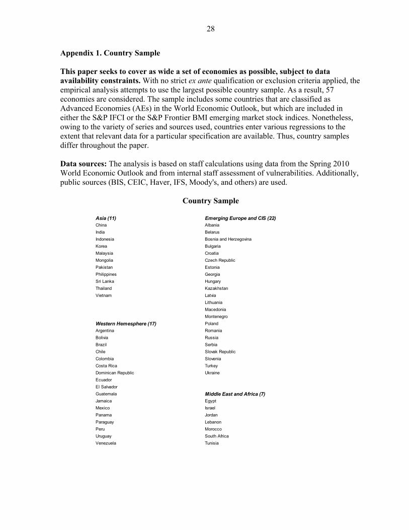
Appendix 1. Country Sample This paper seeks to cover as wide a set of economies as possible, subject to data availability constraints. With no strict ex ante qualification or exclusion criteria applied, the empirical analysis attempts to use the largest possible country sample. As a result, 57 economies are considered. The sample includes some countries that are classified as Advanced Economies (AEs) in the World Economic Outlook, but which are included in either the S&P IFCI or the S&P Frontier BMI emerging market stock indices. Nonetheless, owing to the variety of series and sources used, countries enter various regressions to the extent that relevant data for a particular specification are available. Thus, country samples differ throughout the paper. Data sources: The analysis is based on staff calculations using data from the Spring 2010 World Economic Outlook and from internal staff assessment of vulnerabilities. Additionally, public sources (BIS, CEIC, Haver, IFS, Moody's, and others) are used.

Country Sample

Asia (11) Emerging Europe and CIS (22)China Albania

India Belarus

Indonesia Bosnia and Herzegovina

Korea Bulgaria

Malaysia Croatia

Mongolia Czech Republic

Pakistan Estonia

Philippines Georgia

Sri Lanka Hungary

Thailand Kazakhstan

Vietnam Latvia

Lithuania

Macedonia

Montenegro

Western Hemesphere (17) Poland

Argentina Romania

Bolivia Russia

Brazil Serbia

Chile Slovak Republic

Colombia Slovenia

Costa Rica Turkey

Dominican Republic Ukraine

Ecuador

El Salvador

Guatemala Middle East and Africa (7)Jamaica Egypt

Mexico Israel

Panama Jordan

Paraguay Lebanon

Peru Morocco

Uruguay South Africa

Venezuela Tunisia

29

Appendix 2. List of variables

Pre - Crisis Policy Fundamentals (2007) Measures of trade linkages

1 Exchange rate regime, MCM classification, March-07 1 Exports to advanced economies

2 FX regime, Reinhart Rogoff classification 2 Exports to US, % GDP

3 Inflation targeting framework 3 Manufactures exports

4 Debt stabilizing primary balance 4 Openness (X+M)/GDP

5 Primary gap 5 Export earnings: non-fuel primary commodities

6 External public sector debt 6 Oil exports, % GDP

7 Short-term public debt at residual maturity 7 Fuel exporter dummy

8 Public sector debt linked to FX

9 Primary balance, % GDP Measures of financial linkages

10 Cyclically adjusted primary balance 1 Total external financing requirements, % GDP

11 External debt, total, % GDP 2 Foreign currency loans (% of total loans)

12 External debt, ST, % GDP 3 Loan to deposits ratio

13 External debt, ST at RM, % GDP 4 Claims on private sector, % GDP

14 General gov't debt to GDP 5 Total external financing requirements, % GDP

15 Fiscal impulse 6 Total capital inflows

16 Change in primary balance to GDP 7 Foreign ownership in % of total assets 2007

8 Financial connectedness (Foreign assets + liabilities)/GDP

Measures of pre-crisis overheating Other controls

1 Real GDP growth between 2003 & 2007 1 Population

2 Real domestic credit growth between 2003 & 2007 2 Per capita GDP

3 Percent change in CPI between 2003 & 2007 3 PPP valuation of country GDP

4 Credit to GDP 2007 4 NEER peak to trough percent change

5 Regional dummies

Potential Determinants of Impact on Real Output on EMs During the Crisis 1/

1/ Each one of these indicators was tried in addition to the three core indicators mentioned in Table 2 in the text to check the robustness of results presented in the text. See also Berkmen and others (2009) for a further list of possible explanatory variables.

Appendix 3 – Reserve Robustness with Alternative Control Variables Table A1 - Dependent Variable: Peak to Trough Growth (percent)

(1) (2) (3) (4) (5) (6) (7) (8) (9) (10) VARIABLES <100 >100 <100 >100 <100 >100 <100 >100 <100 >100

Reserves/GDP 0.645*** -0.066 0.710*** -0.003 0.640** -0.008 0.605*** -0.046 0.683*** -0.012 (0.149) (0.058) (0.158) (0.062) (0.200) (0.059) (0.142) (0.041) (0.190) (0.059) Short-term Debt/GDP -0.136 -0.315*** -0.197 -0.371*** -0.108 -0.361*** -0.010 -0.088 -0.170 -0.383*** (0.292) (0.092) (0.178) (0.102) (0.203) (0.104) (0.214) (0.121) (0.193) (0.103) Current Account/GDP 0.834** -0.001 0.581* -0.033 0.825** -0.040 0.966** -0.007 0.857** -0.007 (0.324) (0.079) (0.287) (0.146) (0.297) (0.105) (0.302) (0.064) (0.355) (0.079) Credit/GDP -0.023 0.035* (0.092) (0.019) Dom demand/GDP -0.248 -0.017 (0.204) (0.073) Ln PPP GDP 1.000 0.243 (2.157) (0.657) Ln per capita GDP -4.375 -2.920*** (2.859) (0.782) Credit growth 0.002 -0.007*** (0.010) (0.002) Constant -8.075* -0.957 14.848 2.042 -15.162 -1.115 29.171 23.141*** -9.573 1.258 (3.967) (2.066) (20.288) (7.173) (11.754) (3.398) (25.141) (5.887) (5.455) (2.129) Observations 14 26 14 26 14 26 14 26 14 26 R-squared 0.701 0.368 0.721 0.298 0.708 0.303 0.756 0.551 0.700 0.366

Robust standard errors in parentheses *** p<0.01, ** p<0.05, * p<0.1

31

Table A2 - Dependent Variable: Deviation of Peak to Trough Growth from Pre-Crisis Trend Growth (percent) (1) (2) (3) (4) (5) (6) (7) (8) (9) (10) VARIABLES <100 >100 <100 >100 <100 >100 <100 >100 <100 >100 Reserves/GDP 0.956*** -

0.141**1.007*** -0.031 0.901*** -0.037 0.907*** -0.074 0.972*** -0.050

(0.179) (0.060) (0.201) (0.073) (0.239) (0.068) (0.183) (0.051) (0.231) (0.058) Short-term Debt/GDP

-0.243 -0.353**

-0.286 -0.456*** -0.127 -0.437*** -0.108 -0.187 -0.258 -0.478***

(0.349) (0.127) (0.219) (0.141) (0.199) (0.139) (0.254) (0.174) (0.225) (0.130) Current Account/GDP

1.044** -0.003 0.798* -0.078 1.032** 0.003 1.171** -0.015 1.049** -0.013

(0.382) (0.085) (0.356) (0.206) (0.337) (0.162) (0.364) (0.109) (0.422) (0.077) Credit/GDP -0.011 0.060** (0.111) (0.025) Dom demand/GDP -0.243 -0.044 (0.226) (0.083) Ln PPP GDP 2.187 -0.173 (2.329) (0.729) Ln per capita GDP -4.143 -2.645** (3.048) (1.134) Credit growth 0.001 -0.014*** (0.011) (0.003) Constant -14.956*** -3.630 8.037 2.968 -28.513** -0.524 20.835 19.195** -15.606** 0.497 (4.304) (2.804) (22.940) (7.579) (11.719) (4.674) (26.732) (8.333) (6.575) (2.539) Observations 14 26 14 26 14 26 14 26 14 26 R-squared 0.739 0.429 0.752 0.297 0.770 0.296 0.771 0.428 0.738 0.478 Robust standard errors in parentheses *** p<0.01, ** p<0.05, * p<0.1

32

Table A3 - Dependent Variable: Growth in 2008Q4 – 2009Q1 (percent) (1) (2) (3) (4) (5) (6) (7) (8) (9) (10) VARIABLES <100 >100 <100 >100 <100 >100 <100 >100 <100 >100 Reserves/GDP 0.387** -0.039 0.428** -0.020 0.394** 0.000 0.352** -0.032 0.389** -0.001 (0.134) (0.058) (0.133) (0.053) (0.160) (0.056) (0.123) (0.042) (0.148) (0.054) Short-term Debt/GDP

-0.114 -0.321*** -0.147 -0.301*** -0.124 -0.353*** -0.025 -0.139 -0.120 -0.350***

(0.184) (0.082) (0.131) (0.098) (0.172) (0.095) (0.151) (0.130) (0.137) (0.103) Current Account/GDP

0.596** -0.097 0.367** 0.043 0.595** -0.076 0.677** -0.100 0.587** -0.103

(0.222) (0.063) (0.157) (0.122) (0.218) (0.088) (0.212) (0.064) (0.248) (0.068) Credit/GDP -0.004 0.022 (0.057) (0.019) Dom demand/GDP -0.227 0.108 (0.136) (0.077) Ln PPP GDP -0.062 -0.221 (1.662) (0.637) Ln per capital GDP -2.645 -2.267*** (2.175) (0.797) Credit growth -0.001 0.001 (0.007) (0.002) Constant -4.763 0.325 17.068 -9.915 -4.597 2.378 18.239 18.865*** -4.864 1.035 (3.129) (1.982) (13.339) (7.909) (9.912) (3.010) (19.524

) (5.652) (3.584) (2.162)

Observations 14 26 14 26 14 26 14 26 14 26 R-squared 0.700 0.409 0.734 0.408 0.700 0.383 0.738 0.542 0.700 0.378 Robust standard errors in parentheses *** p<0.01, ** p<0.05, * p<0.1

33

Table A4 – Dependent Variable: Deviation of Peak to Trough Growth from Pre-Crisis Trend Growth (growth_4) (1) (2) (3) (4) (5) (6) (7) VARIABLES/ Res/Std

All EMs

<100 >100 <150 >150 <median >median

Reserves/GDP 0.027 0.860*** -0.043 0.689*** -0.100** 0.670* 0.052 (0.080) (0.227) (0.065) (0.170) (0.038) (0.360) (0.177) Short-term Debt/GDP -0.424*** 0.012 -0.411*** -0.373** -0.878*** -0.562*** -0.443** (0.111) (0.186) (0.145) (0.177) (0.110) (0.135) (0.198) Current Account/GDP 0.059 1.101*** -0.055 0.546* 0.155*** 0.007 0.072 (0.154) (0.277) (0.141) (0.314) (0.046) (0.291) (0.134) Log(Population) 0.358 3.154 0.304 (0.648) (2.322) (0.495) Constant -4.550 -27.060*** -2.762 -13.045*** 3.755** -9.316* -4.114 (3.640) (6.216) (3.390) (3.797) (1.341) (4.389) (7.209) Observations 40 14 26 23 17 19 21 R-squared 0.493 0.802 0.302 0.612 0.828 0.534 0.497 Robust standard errors in parentheses *** p<0.01, ** p<0.05, * p<0.1

34

Table A5 – Dependent Variable: Growth in 2008Q4 – 2009Q1 (growth_1) (1) (2) (3) (4) (5) (6) (7) VARIABLES/ Res/Std

All EMs

<100

>100

<150

>150

<median

>median

Reserves/GDP 0.008 0.377** -0.004 0.259** -0.002 0.368 0.021 (0.058) (0.164) (0.054) (0.119) (0.043) (0.249) (0.103) Short-term Debt/GDP -0.309*** -0.082 -0.335*** -0.138 -0.677*** -0.245*** -0.410*** (0.059) (0.211) (0.098) (0.098) (0.124) (0.064) (0.101) Current Account/GDP -0.009 0.603** -0.127* 0.400** -0.048 0.067 -0.091 (0.094) (0.210) (0.066) (0.156) (0.071) (0.101) (0.081) Log(Population) -0.071 0.445 0.201 (0.481) (1.829) (0.429) Constant 0.903 -6.598 0.289 -4.473* 3.396** -3.992 1.091 (1.886) (7.002) (1.971) (2.487) (1.275) (3.250) (3.941) Observations 40 14 26 23 17 19 21 R-squared 0.488 0.703 0.383 0.599 0.725 0.417 0.621 Robust standard errors in parentheses *** p<0.01, ** p<0.05, * p<0.1