The Impact of the Assimilation of Aquarius Sea Surface ... DOI:10.1029/, The Impact of the Assimilation of Aquarius Sea ... SSS data may not be appropriate for mesoscale or regional

JOURNAL OF GEOPHYSICAL RESEARCH, VOL. ???, XXXX, DOI:10.1029/,

The Impact of the Assimilation of Aquarius Sea

Surface Salinity Data in the GEOS Ocean Data

Assimilation SystemG. Vernieres,

1,2R. Kovach,

1,2C. Keppenne,

1,2S. Akella,

1,2L. Brucker,

3,4E.

Dinnat,3,5

1Science Systems and Applications, Inc.,

Lanham, Maryland, USA.

2Global Modeling and Assimilation Office,

NASA Goddard Space Flight Center,

Greenbelt, Maryland, USA.

3NASA GSFC, Cryospheric Sciences

Laboratory, Code 615, Greenbelt, 20771

MD, U.S.A.

4Goddard Earth Sciences Technology and

Research Studies and Investigations,

Universities Space Research Association,

Columbia, MD 21044-3432 U.S.A.

5Chapman University, Orange, CA 92866,

USA

D R A F T March 27, 2014, 9:56am D R A F T

https://ntrs.nasa.gov/search.jsp?R=20140012074 2018-05-23T22:44:27+00:00Z

X - 2 VERNIERES ET AL.: ASSIMILATION OF AQUARIUS SSS IN GEOS

Abstract. Ocean salinity and temperature differences drive thermoha-

line circulations. These properties also play a key role in the ocean-atmosphere

coupling. With the availability of L-band space-borne observations, it becomes

possible to provide global scale sea surface salinity (SSS) distribution. This

study analyzes globally the along-track (Level 2) Aquarius SSS retrievals ob-

tained using both passive and active L-band observations. Aquarius along-

track retrieved SSS are assimilated into the ocean data assimilation compo-

nent of Version 5 of the Goddard Earth Observing System (GEOS-5) assim-

ilation and forecast model. We present a methodology to correct the large

biases and errors apparent in Version 2.0 of the Aquarius SSS retrieval al-

gorithm and map the observed Aquarius SSS retrieval into the ocean mod-

els bulk salinity in the topmost layer. The impact of the assimilation of the

corrected SSS on the salinity analysis is evaluated by comparisons with in-

situ salinity observations from Argo. The results show a significant reduc-

tion of the global biases and RMS of observations-minus-forecast differences

at in-situ locations. The most striking results are found in the tropics and

southern latitudes. Our results highlight the complementary role and prob-

lems that arise during the assimilation of salinity information from in-situ

(Argo) and space-borne surface (SSS) observations


VERNIERES ET AL.: ASSIMILATION OF AQUARIUS SSS IN GEOS X - 3

1. Introduction

Oceans are large and key elements of the Earths climate system. Among the geophysical

properties characterizing them, salinity and temperature are important. Together, they

control the density of seawater, and therefore the thermohaline circulation. Thus, these

oceanic properties may influence regional climate and weather patterns. While sea surface

temperature (SST) is a key component in air-sea exchanges of heat, sea surface salinity

(SSS) is required for the determination of surface density which dictates the formation of

water masses [Dickson et al., 1988] and therefore has a significant influence on the global

ocean circulation at large spatio-temporal scales [Swift and McIntosh, 1983; Lagerloef ,

2002; Lagerloef et al., 2008]. It has also been argued that a proper estimation of SSS is

required for the closure of the marine hydrological budget [Lagerloef et al., 2008], since

salinity variability is correlated with the net evaporation minus precipitation. Therefore,

retrieving SSS at global scale opens the possibility of using surface salinity to constrain

the estimation of air-sea freshwater uxes, and improve our understanding of the ocean-

atmosphere coupling.

SSS is routinely monitored in the upper 10 m by a series of Argo buoys/profiling floats.

However, these in-situ measurements sample only a small fraction of the ocean, and then

only infrequently [Freeland and Co-Authors , 2010]. SSS measurements are also often col-

lected from ships along shipping routes. Recently, the use of gliders increased, but these

measurements remain localized and sporadic. Since 2009, two satellite missions started

operating: the European Space Agency (ESA) Soil Moisture Ocean Salinity (SMOS) mis-

sion, and the Aquarius/SAC-D mission developed collaboratively between the U.S. Na-



tional Aeronautics and Space Administration (NASA) and the Argentine space agency,

Comision Nacional de Actividades Espaciales (CONAE). These missions operate L-band

(∼ 1.4 GHz) sensors, and provide SSS products following for instance the method de-

scribed in Wentz and Le Vine [2012]; Le Vine et al. [2011]; ? for the Aquarius products.

These satellite observations provide global and synoptic-scale SSS data, which constitute

major contributions to the ocean observing system.

Satellite SSS retrievals are performed with a 0.2 psu precision in the tropical waters

and small biases. However, significant biases have been identified between the satellite

retrievals and in-situ measurements at higher latitudes (Boutin et al. [2013], [Lagerloef

et al., 2013]). Therefore, the use of satellite SSS retrievals by itself may be more challenging

at high latitudes, in cold waters with rough surfaces. This limitation can be tackled

using satellite retrievals in conjunction with in-situ measurements and a data assimilation

system.

Tranchant et al. [2008] conducted Observing System Simulation Experiments (OSSEs)

using simulated Level 2 SMOS and Aquarius SSS data in the Mercator Ocean multivariate

assimilation system. They obtained significant reductions in the mean (from ∼ 0.15 to

∼ 0.05 ) and variance (from ∼ 0.3 to ∼ 0.1) for the difference between their reference

(assimilating all operational observations) and assimilated simulated space-borne SSS.

Differences were the largest: (i) in high latitudes where satellite observation errors are

highest; (ii) in regions of high variability (e.g. the Gulf Stream); and (iii) near coastlines

where SSS is significantly impacted by river runoff.

Hackert et al. [2011] showed that assimilating SSS improved seasonal forecasts of SST

in the western equatorial Pacific, in both the South Pacific Convergence Zone (SPCZ) and



the Intertropical Convergence Zone (ITCZ). Specically for the El Nino Southern Oscilla-

tion (ENSO), they showed that the root-mean-square (RMS) error in 6–12 months leads

forecasts for December-to-March was reduced by 0.3oC – 0.6oC using initial conditions

that assimilated SSS along with other observations (including sub-surface temperature

and salinity) into their intermediate coupled model.

More recently, Hackert and Busalacchi [2012] obtained similar results, namely, coupled

experiments initialized by assimilation of satellite SSS outperformed in-situ SSS assimi-

lation. In addition, ocean analyses that assimilated both Aquarius and SMOS SSS data

led to lower RMS forecast errors than forecasts initialized from ocean analyses that as-

similated Aquarius or SMOS alone.

Therefore, the benefits of assimilating SSS have been shown. Nevertheless, these pre-

vious studies [e.g. Tranchant et al., 2008; Hackert et al., 2011; Hackert and Busalacchi ,

2012] also emphasized with synthetic observations the challenges in assimilating real-time

satellite SSS and in-situ salinity data.

To advance on these studies, the objective of this work is to assimilate globally the

version 2.0 of the Aquarius Level 2 retrieved SSS in NASA GEOS-5 iODAS. This is

done for the first time and enables us to overcome some of the challenges previously

identified. Section 2 briey outlines important features of the Aquarius SSS retrievals and

issues relevant to using retrieved data in assimilation. The GEOS system and iODAS

are described in Section 3. The experimental setup is described in Section 4, and Section

5 discusses the results of the assimilation experiments; finally, conclusions are drawn in

Section 6.



2. Aquarius SSS data, retrieval and preprocessing

Passive microwave (L-band) retrieval of SSS from space is based on the fact that the

dielectric constant of sea water depends on the surface salinity [Klein and Swift , 1977;

Swift and McIntosh, 1983; Ulaby et al., 1986; Le Vine et al., 2007]. At the low microwave

frequencies of the L band (Aquarius frequency is centered around 1.413 GHz) the ob-

served brightness temperature (TB) is a function of SST and sea surface emissivity. The

emissivity directly depends on SSS, and also on other properties (such as roughness from

surface wind, waves, swells, currents and SST). At L band, the sensitivity δTB/δSSS is

significantly higher than it would be at higher frequencies usually used in remote sensing.

Hence if SST and surface emissivity are accurately known, it is possible to obtain SSS

information with an accuracy suitable for oceanographic studies. In this regard, unlike

the SMOS mission, the Aquarius/SAC-D mission has an onboard scatterometer to simul-

taneously quantify surface roughness. Other important effects that impact SSS retrievals

are: Faraday rotation, solar and galactic radiation, etc; see Le Vine et al. [2011] and Din-

nat and Vine [2008] for further details. The method used to retrieve SSS from Aquarius

observations is described in Wentz and Le Vine [2012]; Le Vine et al. [2011]; Piepmeier

et al. [2012]. The Aquarius/SAC-D mission was designed to provide SSS with an accuracy

of 0.2 Practical Salinity Units (PSU) on a global monthly RMS error.

Difficulties in the retrieval of SSS primarily relevant to this study are as follows:

1. Observations are made with a large footprint ranging (along x across track) from 76

km x 94 km to 96 km x 156 km. Due to these low spatial resolution observations, the

SSS data may not be appropriate for mesoscale or regional studies. Heterogeneities in



the footprint, either corrected in part (e.g. land contamination) or not corrected (e.g. ice

contamination), may reduce the quality of the SSS retrievals.

2. The measurement sensitivity is proportional to the SST [Lagerloef et al., 2013], so

that at high latitudes, where SST is the lowest, large SSS retrieval errors are expected.

3. At 1.4 GHz the penetration depth of the electromagnetic radiation into the upper

ocean is of the order of 1 cm, which implies that the measured TB relates to the salinity

very close to the surface. However, the satellite SSS retrieval is based on calibration using

in-situ buoys with salinity sensors at a meter or deeper. In other words, the difference

between bulk and surface salinity is neglected in the retrieval.

4. Uncertainties in the SST, roughness and ocean emissivity may induce errors in the

retrieval of SSS, therefore it is important to characterize and to quantify them.

2.1. Issues regarding the retrieval in the assimilation context

The left top panel of Figure 1 illustrates the global probability density functions (PDFs)

of the retrieved SSS (blue) and collocated in-situ observations (red) of salinity in the upper

10 meters of the ocean. The differences between the two PDFs are due to large biases

and errors in the retrieval algorithm and due to instrumental calibration problems, as

documented in Lagerloef et al. [2013]. The fact that the in-situ observations used for the

comparison are those of bulk salinity, defined as the average salinity in the upper 10 m

of the ocean, may contribute to some of the differences. Thus, the in-situ measurement

may differ signicantly from the retrieved SSS in strongly stratied regions.

The left panel of Figure 1 also shows a scatter plot of satellite SSS versus in-situ salinity.

While the correlation is relatively high (0.8), implying that the retrieval is capturing the



proper variability, the root mean square error (RMSE) is too high to be usable in a state

estimation framework.

Because of these problems, a mapping of the retrieved SSS into the upper ocean salinity

will be required for assimilation purposes. Further investigation also shows significant

biases, unique to the instrument and based on whether the orbit is ascending or descending

(see Figure 3 and 4 as well as Lagerloef et al. [2013]).

2.2. Preprocessing

We address the problem of significant differences between the retrieved SSS and in-situ

observations of bulk salinity by developing a pre-processing algorithm to recalibrate the

SSS to the model-valued bulk surface salinity. This is done by constructing a real valued

function φ that maps SSS into bulk salinity. This function (φ) is approximated with a

Feed Forward Artificial Neural Network (FFANN), which is commonly used as a universal

function approximator [Kohonen, 1982; Hopfield , 1982; Krasnopolsky , 2007]. The FFANN

outputs a bulk salinity. Its input (the transposed vector xT ) is defined as

xT = [longitude, latitude, k, SST, SSS] (1)

where k is an integer corresponding to the instrument and orbit type (k = 1, .., 6), SST

is the ancillary sea surface temperature and SSS is the retrieved sea surface salinity from

Aquarius. To accelerate the convergence of the training, the input x is scaled by removing

the mean and dividing by the standard deviation observed in the training set for each

element of x. The targets used to train the network consist of in-situ measurements of

bulk salinity from Argo from October 2011 to the end of 2012. A total of 51, 798 surface

salinity measurements were used, which corresponds to approximately 20% of the in-situ



surface observations and 0.4% of the Aquarius SSS observations. The validation data set

is constructed in the same way but only using Argo and Aquarius measurements from

2013 (January first to the end of August). The size of the validation set is 24, 498. The

FFANN is formally written as follows:

φ(x;α) = bout +

nh∑j=1

woutj g

(bin +

n∑i=1

winjixi

), (2)

where α is a vector containing the parameters of the FFANN (bout, bin and weights win

and wout) and g is the sigmoid function (g(t) = 1/(1+exp(−t))). Training of the FFANN

involves finding the set of weights α that minimizes the error function:

F (α) =1

2

Nt∑i=1

σi

(φ(xi;α)− yi

)2

(3)

where yi is an in-situ measurement of bulk salinity, xi is the closest Aquarius measurement

to yi (within a 4 degree box in longitude and latitude and inside of a 24 hour window)

and σi is a weight related to the distance between the Aquarius measurement and the in-

situ observation. The minimization uses the Newton conjugate gradient method, which

requires the following Jacobian of the error function:

Jk =∂F (α)

∂αk

=Nt∑i=1

σi

(φ(xi;α)− yi

)∂φ(xi;α)

∂αk

(4)

To speed up convergence of the training process, the error function in equation (3) and

the analytical Jacobian (4) are distributed across several CPUs using a red-black ordering

of the summations in (3) and (4). For the purpose of our experiments, this methodology

showed good scalability, up to approximately 128 CPUs. The middle panel of Figure 1

illustrates the topology of the FFANN with the forward propagation of the inputs and

single output. The right panel demonstrates the improvement on the shape of the PDF

when preprocessing the retrieved SSS. The correlation with in-situ observations used for



the training is now 0.98 with a RMSE of 0.21 whereas the raw retrieval had a correlation

of 0.82 and RMSE of 0.73. The validation data set uses 24, 498 in-situ measurements

between January and August 2013. The statistics for the validation dataset, shown on

the right hand side of Figure 2, demonstrate the generalization of the FFANN since the

correlation and RMSE are quite similar to the one observed for the training data set.

3. The GEOS iODAS system

The GEOS integrated Ocean Data Assimilation System (GEOS iODAS) is a system for

both ocean and sea-ice data assimilation. It is integrated within the broader GEOS model

and data assimilation system using the Earth System Modeling Framework (ESMF). The

iODAS has been tuned to work with the Modular Ocean Model Version 4.1 (MOM4.1;

Griffies et al. [2005]) developed by the NOAA Geophysical Fluid Dynamics Laboratory

(GFDL) and the CICE model [Hunke and Lipscomb, 2010] developed by the Los Alamos

National Laboratory. The primary objective of the system is to produce fields of tempera-

ture, salinity, currents, sea surface height, sea ice thickness and concentration to initialize

short-term climate forecasts.

3.1. Model and forcing

The GEOS model configuration used in this study uses prescribed surface forcing

fields from NASAs Modern-Era Retrospective Analysis for Research and Applications

(MERRA) [Rienecker et al., 2011]. The skin layer is provided with specified hourly fields

of: 10-meter air temperature, 10-meter specific humidity, 10-meter winds, sea level pres-

sure, surface absorbed long-wave radiation, surface incoming short-wave flux, precipitation

(rain and snow) and river run-off.



The nominal resolution of the ocean grid is 1/2o, with a meridional equatorial refinement

to 1/4o. The configuration uses a regular Cartesian grid south of 65N, and curvilinear

north of 65N, with two poles located on land to eliminate the problem of vanishing cell

area at the geographic North Pole. The ocean topography is derived from the ETOPO5

(Data Announcement 88-MGG-02, Digital relief of the Surface of the Earth. NOAA,

National Geophysical Data Center, Boulder, Colorado, 1988) data set. The grid includes

40 unevenly distributed levels in the vertical.

3.2. The iODAS, brief description and configuration

The iODAS is a sequential ensemble assimilation software system that includes a wide

range of algorithm implementations, from simple optimal interpolation (OI: Eliassen

[1954]) to ensemble data assimilation methods including ensemble Kalman [Evensen, 2003]

and particle filters. The results presented here use the iODAS ensemble optimal interpo-

lation [Oke et al., 2010; Wan et al., 2009] implementation where the time dependency of

the covariances is neglected and the model error covariances are estimated from an en-

semble of sample error fields. The ensemble is assembled from a suite of seasonal hindcast

anomalies. The reader is refereed to Keppenne et al. [2008] and Vernieres et al. [2012] for

further details.

4. The Experimental set up

We present results from five simulations, each starting on November 3, 2011 from the

same initial conditions and using the same external MERRA forcing as are used for the

GMAO seasonal forecast. Two simulations serve as references: one does not include any

assimilation and is referred to as BASENODA. The other assimilates upper ocean in-situ



salinity observations (from the surface to 100m deep) and is referred to as BASEDA. The

third simulation assimilates the Aquarius retrieval without any reprocessing, it is meant

to illustrates the difficulties faced when assimilating the raw data set, and is referred

to as RAW. The fourth simulation assimilates the Aquarius retrieval, reprocessed with

the FFANN neural network described above and is referred to as ANN. Finally the ALL

experiment assimilates the same upper ocean in-situ salinity observations as BASEDA

and the same Aquarius salinity as ANN. The assimilation window is set to 24 hours for

all observations. A summary of the experiments is given in Table 1.

5. Results

While BASEDA does not correspond to the truth, it was our best estimate of the state

of the upper ocean salinity prior to the advent of remotely sensed SSS. The top panels of

Figure 5 show the mean bulk salinity difference between RAW and BASEDA (panel (a)),

ANN and BASEDA (panel (b)) and ALL and BASEDA (panel (c)). Panel (a) shows the

largest differences, while differences between panels (b) and (c) are much smaller, implying

that the 2012 mean bulk salinity in ANN and ALL are dominated by the assimilation of the

reprocessed Aquarius SSS and are also very similar to the climatology of BASEDA. While

the RAW biases are mostly corrected when the reprocessed Aquarius SSS are assimilated

(panel (b)), some significant differences remain. For example, the negative bias in the

Bay of Bengal and just north of the Indonesian throughflow is reduced relative to RAW.

but still shows surface waters that is fresher than that estimated by assimilating only

in-situ observations. The RMS differences between experiments with respect to BASEDA

are shown in panels (d), (e) and (f). Again, the smallest RMS difference is obtained for

ALL and ANN, and the differences shown in panels (e) and (f) are minimal. However,



in places of high variability and where runoff is important, large RMS differences are

apparent, indicating that the information in the remotely sensed SSS differs from that

in the in-situ observations. The bottom panels (g), (h) and (i) show the correlations

between each of RAW, ANN and ALL with BASEDA. Ignoring latitudes above 70 N and

below 70 S where observations are sparse, relatively large correlations with BASEDA are

observed in the tropics for RAW, while ANN shows high correlation with BASEDA in

most regions and is again very similar to the correlations between ALL and BASEDA. The

contrast between the first and second columns of Figure 5 illustrate clearly the difficulties

of assimilating the raw Aquarius retrieval directly and shows the significant improvement

from assimilating the reprocessed SSS.

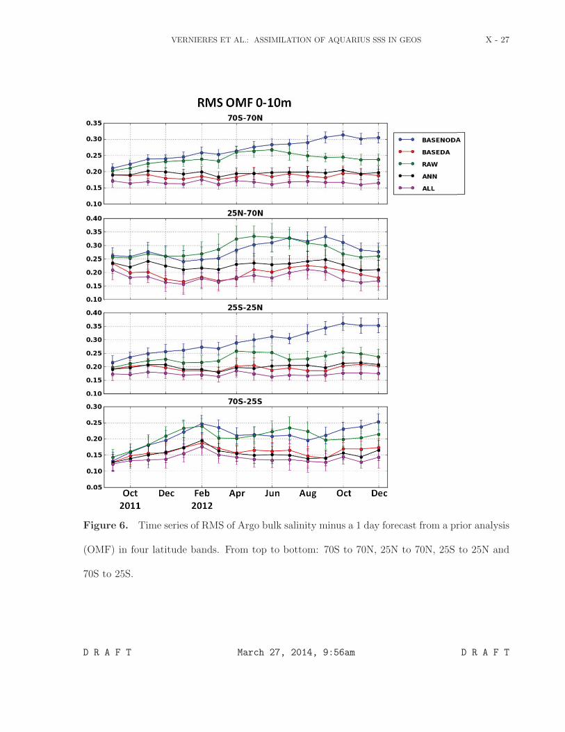
Figure 6 shows the RMS of the salinity observation minus forecast (OMF) at Argo

locations, where OMF is defined as the difference between the in-situ bulk salinity ob-

servations and the one-day-lead model forecast from the previous analysis. The OMF

statistics shed light on the performance of each experiment and help further quantify the

impact of SSS assimilation. The colored dots correspond to the monthly mean OMFs

and the width of the error bar represents two standard deviations of the OMFs within

that month. The error bars reflect the confidence in the mean OMF. The results are

much like one would expect from a high quality data set: more observations results in a

better estimate of the state of the ocean. In the top panel of Figure 6, which represents

the nearly global (70S to 70N) statistics, the smallest RMS OMFs are observed in ALL.

This is an important result that implies that the reprocessed Aquarius SSS and in-situ

observations are both consistent and complementary. The Aquarius SSS provides a better

estimate of the Argo data available at the next analysis time than using Argo data alone



because the Argo locations change with every assimilation cycle. The best performance

for the ANN experiment is observed in the tropics and south of 25S, where RMS OMFs

are generally smaller than in BASEDA (see the 2 bottom panels of Figure 6) and at times

is not significantly different from ALL.

Figure 7 illustrates the same geographical decomposition, but looking at the vertical

distribution of the RMS OMF for 2012 only. It shows that ANN is an improvement over

BASENODA in all three regions, while ANN does better or similar to BASEDA between

70S and 25S. The influence of the surface salinity information extends down the water

column and improves the analysis and forecast away from the surface. This is further

illustrated in Figure 8, which depicts the differences in salt content in the upper 100

m between BASENODA and BASEDA (top panel) and ANN and BASEDA (bottom

panel). The improvement caused by assimilating the reprocessed SSS is again clear in

most regions.

To further investigate the vertical influence of assimilating the reprocessed Aquarius

SSS, we compare the 2012 mean subsurface salinity of BASENODA and ANN to the

GMAO ocean reanalysis, henceforth referred to as MERRA-Ocean [Vernieres et al., 2012].

MERRA-Ocean assimilates all available observations, altimeter, SST and in-situ profiles

of salinity and temperature. Because it involves a 5-day assimilation window and a clima-

tology constraint on bulk salinity, the upper ocean salinity of MERRA-Ocean is further

away from the observations than BASEDA. However, it includes observations below 100

m deep and therefore, is more realistic than BASEDA below the mixed layer.

Figure 9 shows salinity cross sections of the zonal-mean differences in 2012 for the

Pacific (top), Atlantic (middle) and Indian (bottom) ocean. The left panels show the



differences between BASENODA and MERRA-Ocean while the right panels show the

differences between ANN and MERRA-Ocean. In the Pacific ocean, the positive impact

of assimilating Aquarius data is seen down to approximately 200m in the tropics, and

down to 100m in the region of the Antarctic circumpolar current. No positive effect is

observed above 50N where both BASEDA and ANN are saltier that MERRA-Ocean.

Improvement in the Atlantic ocean is more subtle but still visible between 65S and 40S

and is also limited to shallower regions. In the Indian Ocean, ANN is consistently closer

to MERRA-Ocean below the surface than BASENODA is, with impact observed down to

at most 200m in the high latitudes.

6. Summary

We have presented a methodology to correct some of the biases and errors observed

in the retrieved SSS from Aquarius. We showed that while the training data set only

included in-situ observations from 2011 and 2012, the FFANN also corrected the Aquarius

SSS for year 2013, which implies that the neural network has learned a correction that

can be generalized. Several different network topologies were tested, mainly by changing

the number of inputs. A simple ”cold-water” network (not shown in this study) using

only Aquarius SSS and SST colder than 10 ◦C as input, did very well at correcting the

large biases and errors observed in the southern latitude. However it did poorly in the

northern latitude where a proper correction to salinity requires a knowledge of the position

(longitude and latitude). It is unclear at this point if the large errors and biases observed

are due to problems in the calibration, in the physics of the retrieval, or simply that the

bulk salinity is very different to the surface salinity presumably estimated by Aquarius.



Assimilating the reprocessed retrieval showed a reduction in RMS OMF in most geo-

graphical regions and improved the salinity estimate in the upper ocean to at least 200 m.

We also showed that assimilating in-situ and Aquarius measurements together improved

the model short-term forecast at Argo locations, suggesting that Aquarius adds informa-

tion to the in-situ ocean observing system. Future work will examine the influence of

this new data stream on estimates of the upper ocean heat and salt budgets. We also

plan to examine the impact of this new data set on long range forecast (seasonal and

sub-seasonal).

Acknowledgments. This work was supported by NASAs Modeling Analysis and Pre-

diction Program under WBS 802678.02.17.01.25. The computational resources for the

runs was provided by the NASA Center for Climate Simulation (NCCS). Yuri Vikhliaev,

Max Suarez and Bin Zhao of GMAO integrated MOM5 and CICE into the GEOS-5 mod-

eling system and configured the system used in this study. Their support is gratefully

acknowledged. The authors would also like to thank Michele Rienecker for her many

insightful comments.

References

Boutin, J., N. Martin, G. Reverdin, X. Yin, and F. Gaillard (2013), Sea surface freshening

inferred from smos and argo salinity: impact of rain, Ocean Science, 9 (1), 183–192, doi:

10.5194/os-9-183-2013.

Dickson, R. R., J. Meincke, S.-A. Malmberg, and A. J. Lee (1988), The great salinity

anomaly in the Northern North Atlantic 19681982 , Progress in Oceanography, 20 (2),

103 – 151, doi:10.1016/0079-6611(88)90049-3.



Dinnat, E. P., and D. M. L. Vine (2008), Impact of sun glint on salinity remote sensing:

An example with the aquarius radiometer., IEEE T. Geoscience and Remote Sensing,

46 (10), 3137–3150.

Eliassen, A. (1954), Provisional report on calculation of spatial covariance and autocorre-

lation of the pressure field, Inst. Weather and Clim. Res., Acad. Sci., Oslo, Tech. Rep,

5.

Evensen, G. (2003), The ensemble kalman filter: theoretical formulation and practical

implementation, Ocean Dynamics, 53 (4), 343–367, doi:10.1007/s10236-003-0036-9.

Freeland, H., and Co-Authors (2010), Argo - A Decade of Progress, in Proceedings of

OceanObs’09: Sustained Ocean Observations and Information for Society, vol. 2, edited

by H. D. Hall, J. and E. Stammer, D., ESA Publication.

Griffies, S. M., A. Gnanadesikan, K. W. Dixon, J. P. Dunne, R. Gerdes, M. J. Harrison,

A. Rosati, J. L. Russell, B. L. Samuels, M. J. Spelman, M. Winton, and R. Zhang

(2005), Formulation of an ocean model for global climate simulations, Ocean Science,

1 (1), 45–79, doi:10.5194/os-1-45-2005.

Hackert, E., and A. J. Busalacchi (2012), Impact of Satellite SSS

on ENSO Forecasts for the Tropical Indo-Pacific, AGU poster,

http://fallmeeting.agu.org/2012/files/2012/11/Fall-AGU-poster2.pdf.

Hackert, E., J. Ballabrera-Poy, A. J. Busalacchi, R.-H. Zhang, and R. Murtugudde

(2011), Impact of sea surface salinity assimilation on coupled forecasts in the

tropical pacific, Journal of Geophysical Research: Oceans, 116 (C5), n/a–n/a, doi:

10.1029/2010JC006708.



Hopfield, J. J. (1982), Neural networks and physical systems with emergent collective

computational abilities, Proceedings of the National Academy of Sciences, 79 (8), 2554–

2558.

Hunke, C., E., and W. H. Lipscomb (2010), CICE: the Los Alamos Sea Ice Model Doc-

umentation and Software Users Manual Version 4.1, Tech. Rep. LA-CC-06-012, Los

Alamos National Laboratory, Los Alamos National Laboratory Los Alamos NM 87545.

Keppenne, C. L., M. M. Rienecker, J. P. Jacob, and R. Kovach (2008), Error Covariance

Modeling in the GMAO Ocean Ensemble Kalman Filter, Monthly Weather Rev, 136 (8),

2964, doi:10.1175/2007MWR2243.1.

Klein, L., and C. Swift (1977), An improved model for the dielectric constant of sea water

at microwave frequencies, Antennas and Propagation, IEEE Transactions on, 25 (1),

104–111, doi:10.1109/TAP.1977.1141539.

Kohonen, T. (1982), A simple paradigm for the self-organized formation of structured fea-

ture maps, in Competition and Cooperation in Neural Nets, Lecture Notes in Biomath-

ematics, vol. 45, edited by S.-i. Amari and M. A. Arbib, pp. 248–266, Springer Berlin

Heidelberg.

Krasnopolsky, V. M. (2007), Neural network emulations for complex multidimensional

geophysical mappings: Applications of neural network techniques to atmospheric and

oceanic satellite retrievals and numerical modeling, Reviews of Geophysics, 45 (3), n/a–

n/a, doi:10.1029/2006RG000200.

Lagerloef, G., C. F.R., D. Le Vine, F. Wentz, S. Yueh, C. Ruf, J. Lilly, J. Gunn, Y. Chao,

A. deCharon, A. Feldman, and C. Swift (2008), The Aquarius/SAC-D Mission: De-

signed to meet the salinity remote-sensing challenge, Oceanography, 21 (1), 68–81.



Lagerloef, G., H.-Y. Kao, O. Melnichenko, P. Hacker, E. Hacker, Y. Chao, K. Hilburn,

T. Meissner, S. Yueh, L. Hong, and T. Lee (2013), Aquarius Salinity Validation Analysis,

Tech. Rep. AQ-014-PS-0016, NASA/CONAE.

Lagerloef, G. S. E. (2002), Introduction to the special section: The role of surface salin-

ity on upper ocean dynamics, air-sea interaction and climate, Journal of Geophysical

Research: Oceans, 107 (C12), SRF 1–1–SRF 1–2, doi:10.1029/2002JC001669.

Le Vine, D., G. S. E. Lagerloef, F. Colomb, S. Yueh, and F. Pellerano (2007), Aquarius: An

instrument to monitor sea surface salinity from space, Geoscience and Remote Sensing,

IEEE Transactions on, 45 (7), 2040–2050, doi:10.1109/TGRS.2007.898092.

Le Vine, D., E. Dinnat, S. Abraham, P. De Matthaeis, and F. Wentz (2011), The aquarius

simulator and cold-sky calibration, Geoscience and Remote Sensing, IEEE Transactions

on, 49 (9), 3198–3210, doi:10.1109/TGRS.2011.2161481.

Oke, P. R., G. B. Brassington, D. A. Griffin, and A. Schiller (2010), Ocean data as-

similation: a case for ensemble optimal interpolation, Australian Meteorological and

Oceanographic Journal, 59 (Sp. Iss), 67–76.

Piepmeier, J. R., D. M. LeVine, S. H. Yueh, F. Wentz, and C. Ruf (2012), Aquarius

radiometer performance: Early on-orbit calibration and results.

Rienecker, M. M., M. J. Suarez, R. Gelaro, R. Todling, J. Bacmeister, E. Liu, M. G.

Bosilovich, S. D. Schubert, L. Takacs, G.-K. Kim, S. Bloom, J. Chen, D. Collins,

A. Conaty, A. da Silva, W. Gu, J. Joiner, R. D. Koster, R. Lucchesi, A. Molod,

T. Owens, S. Pawson, P. Pegion, C. R. Redder, R. Reichle, F. R. Robertson, A. G.

Ruddick, M. Sienkiewicz, and J. Woollen (2011), MERRA: NASA’s Modern-Era Retro-

spective Analysis for Research and Applications, Journal of Climate, 24 (14), 3624–3648,



doi:10.1175/JCLI-D-11-00015.1.

Swift, C., and R. McIntosh (1983), Considerations for microwave remote sensing of ocean-

surface salinity, Geoscience and Remote Sensing, IEEE Transactions on, GE-21 (4),

480–491, doi:10.1109/TGRS.1983.350511.

Tranchant, B., C.-E. Testut, L. Renault, N. Ferry, F. Birol, and P. Brasseur (2008),

Expected impact of the future SMOS and Aquarius Ocean surface salinity missions in

the Mercator Ocean operational systems: New perspectives to monitor ocean circulation

, Remote Sensing of Environment, 112 (4), 1476 – 1487, doi:10.1016/j.rse.2007.06.023,

remote Sensing Data Assimilation Special Issue.

Ulaby, F., R. Moore, and A. Fung (1986), Microwave remote sensing: Active and passive,

vol. iii, volume scattering and emission theory, advanced systems and applications, Inc.,

Dedham, Massachusetts, pp. 1797–1848.

Vernieres, G., M. M. Rienecker, R. Kovach, and L. C. Keppenne (2012), The GEOS–

iODAS: Description and Evaluation, Tech. Rep. TM-2012-104606, NASA, National

Aeronautics and Space Administration Goddard Space Flight Center Greenbelt, Mary-

land 20771.

Wan, L., L. Bertino, and J. Zhu (2009), Assimilating altimetry data into a hycom model

of the pacific: Ensemble optimal interpolation versus ensemble kalman filter, Journal of

Atmospheric and Oceanic Technology, 27 (4), 753–765, doi:10.1175/2009JTECHO626.1.

Wentz, F., and D. Le Vine (2012), Aquarius salinity retrieval algorithm (version 2) algo-

rithm theoretical basis document (atbd), Tech. Rep. 082912, RSS Technical Report.



Table 1. Summary of the experiments. The rightmost column is the RMS of in-situ OMF

between 70S and 70N.Experiment Name Observations assimilated rms OMF’sBASENODA None 0.268± 0.03BASEDA In-situ 0.186± 0.005RAW Aquarius SSS (Level 2 version 2.0) 0.239± 0.017ANN Reprocessed Aquarius SSS 0.195± 0.005ALL In-situ and reprocessed Aquarius SSS 0.166± 0.004



Figure 1. Left panel:(bottom right) PDF of bulk in-situ salinity measurements collocated

with the descending orbit of beam 3 of Aquarius SSS. (Top) The PDF of Aquarius SSS (beam 3,

descending orbit) at bulk in-situ measurements location is shown in blue. The red line corresponds

to the PDF from bulk in-situ salinity measurements collocated with Aquarius SSS. (Bottom left)

Scatter plot of a 2D histogram of Aquarius SSS versus bulk in-situ observations, the colors

represents the sample size as a fraction of the total number of observations. The black line

corresponds to the perfect correspondence between Aquarius SSS and bulk in-situ observations.

Middle panel: Topology of the FFANN. The inputs consist of longitude (lon), latitude(lat), doy

of year (doy), SST and Version 2.0 of level 2 retrieved SSS from Aquarius. The single output is

shown on the right and consists of a corrected SSS. Right panel: Same as the left panel but for

the re-processed Aquarius SSS (output of the FFANN).



Figure 2. Same as Figure 1 but for the 2013 validation data set.



Figure 3. Binned Aquarius SSS minus Argo bulk salinity from September 2011 to the end of

December 2012. The bin size is 3x3 degrees. Upper panels correspond to the ascending orbit,

lower panels to the descending orbits. Left panels are beam 1, middle are beam 2 and right are

beam 3.



Figure 4. Same as Figure 3 but for the RMS difference between Aquarius SSS and bulk salinity

from Argo.



Figure 5. Statistics of the bulk salinity difference between RAW and BASEDA (left column)

ANN and BASEDA (middle column) ALL and BASEDA (right column) for 2012. The top row

is the mean, the middle row is the RMS difference and the bottom row is the correlation.



Figure 6. Time series of RMS of Argo bulk salinity minus a 1 day forecast from a prior analysis

(OMF) in four latitude bands. From top to bottom: 70S to 70N, 25N to 70N, 25S to 25N and

70S to 25S.



Figure 7. Vertical distribution of RMS of OMF’s in three different regions: 70S to 25S (left

panel), tropics (middle panel) and 25N to 70N (right panel). Refer to Figure 6 for the color

legend.



Figure 8. Upper 100 meter salinity content difference between BASENODA and BASEDA

(top panel) and ANN and BASEDA (bottom panel)



Figure 9. Climatology of salinity of BASENODA minus MERRA-Ocean (left panels) and

ANN minus MERRA-Ocean (right panels). From top to bottom, Pacific, Atlantic and Indian

ocean.


Documents

The Impact of the Assimilation of Aquarius Sea Surface ... DOI:10.1029/, The Impact of the Assimilation of Aquarius Sea ... SSS data may not be appropriate for mesoscale or regional