Research Report DFE-RR067

The impact of SureStart Local Programmes on five year olds and their families

The National Evaluation of Sure Start (NESS) Team

Institute for the Study of Children, Families and Social Issues,

Birkbeck University of London

This research report was commissioned before the new UK Government took office on 11 May 2010. As a result the content may not reflect current

Government policy and may make reference to the Department for Children, Schools and Families (DCSF) which has now been replaced by the Department

for Education (DFE).

The views expressed in this report are the authors’ and do not necessarily reflect those of the Department for Education.

The National Evaluation of Sure Start Team is based at the Institute for the Study of Children, Families & Social Issues, Birkbeck,

University of London, 7 Bedford Square, London, WC1B 3RA

Core Team Professor Edward Melhuish, Institute for the Study of Children, Families & Social Issues,

Birkbeck (Executive Director)

Professor Jay Belsky, Institute for the Study of Children, Families & Social Issues, Birkbeck (Research Director)

Professor Alastair Leyland, MRC Social & Public Health Sciences Unit, Glasgow (Statistician)

Impact Module Professor Edward Melhuish, Institute for the Study of Children, Families & Social Issues,

Birkbeck (Director)

Professor Angela Anning, Institute for the Study of Children, Families & Social Issues, Birkbeck (Investigator)

Professor Sir David Hall, University of Sheffield (Investigator)

Implementation Module Professor Jane Tunstill, (Director)

Mog Ball (Investigator)

Pamela Meadows, National Institute of Economic & Social Research (Investigator)

Cost Effectiveness Module Pamela Meadows, National Institute of Economic & Social Research (Director)

Local Context Analysis Module Professor Jacqueline Barnes, Institute for the Study of Children, Families & Social Issues,

Birkbeck (Director)

Dr Martin Frost, Birkbeck (Investigator)

Support to Local Programmes on Local Evaluation Module Professor Jacqueline Barnes, Institute for the Study of Children, Families & Social Issues,

Birkbeck (Director)

Data Analysis Team Mark Hibbett, Institute for the Study of Children, Families & Social Issues, Birkbeck Dr Andrew Cullis, Institute for the Study of Children, Families & Social Issues, Birkbeck

ii

THE IMPACT OF SURE START LOCAL PROGRAMMES ON

FIVE YEAR OLDS AND THEIR FAMILIES

Report of the Longitudinal Study of 5-year-old Children and Their Families

EXECUTIVE SUMMARY

Background

The ultimate goal of Sure Start Local Programmes (SSLPs) was to enhance the life chances for young children growing up in disadvantaged neighbourhoods. Children in these communities are at risk of doing poorly at school, having trouble with peers and agents of authority (i.e., parents, teachers), and ultimately experiencing compromised life chances (e.g., early school leaving, unemployment, limited longevity). This has profound consequences not just for the children but for their families, communities, and for society at large. Thus, SSLPs not only aimed to enhance health and well-being during the early years, but to increase the chances that children would enter school ready to learn, be academically successful in school, socially successful in their communities and occupationally successful when adult. Indeed, by improving - early in life- the developmental trajectories of children at risk of compromised development, SSLPs aimed to break the intergenerational transmission of poverty, school failure and social exclusion. Such a strategy was a profound innovation in policy.

SSLPs were strategically situated in areas of high deprivation and they represented an innovative intervention unlike almost any other undertaken to enhance the life prospects of young children in disadvantaged families and communities. One characteristic which distinguished SSLPs from almost all other early interventions evaluated up to the year 2000, was that the programme was area based, with all children under five years of age and their families living in a prescribed area serving as the “targets” of intervention. This was seen as having the advantage that services (e.g. childcare, family support) within a SSLP area would be universally available, thereby limiting any stigma that may accrue from individuals being targeted. In the early years of SSLPs, by virtue of their local autonomy and in contrast to more narrowly-defined

iii

early interventions, SSLPs did not have a prescribed “curriculum” or set of services, especially not ones delineated in a “manualised” form to promote fidelity of treatment to a prescribed model. Instead, each SSLP had extensive local autonomy over how it fulfilled its mission to improve and create services as needed, without specifying how services were to be changed.

From 2005 to 2006, fundamental changes were made in SSLPs, as they came under the control of Local Authorities and were operated as children’s centres (CCs). This modified the service-delivery process in that the guidelines for CCs were more specific about the services to be offered. Nonetheless there is still substantial variation among Local Authorities and areas within Local Authorities in the way the new CC model is implemented. This continues to pose challenges to evaluating their impact, as each SSLP or CC remains unique.

Evaluating SSLP Impact

As part of an assessment of the impact of SSLPs on child and family functioning, the Impact Study of the National Evaluation of Sure Start (NESS) has followed up over 7000 5-year-olds and their families in 150 SSLP areas who were initially studied when the children were 9 months and 3 years old. The 5 year old study followed up a randomly selected subset (79%) of the children and families previously studied at 9 months and 3 years.

The comparison group of Millennium Cohort Study (MCS) children and their families, against which the NESS sample was compared, was selected from the entire MCS cohort. Their selection was based upon identifying and selecting children living in areas with similar economic and demographic characteristics to those in which the NESS sample resided, but which were not SSLP-designated areas and thus did not offer SSLP services. This enabled the NESS research team to make comparisons with children and families from areas as similar as possible to the NESS Impact Study areas to detect the potential effects of SSLPs on children and families.

Methodological Issues

Any effects discerned in the evaluation have to be considered “putative” because the data for the NESS and MCS samples of 5-year olds and their families were collected two years apart and by two different research teams. This makes attributing any discerned SSLP effects to SSLP exposure per se difficult, as they could potentially reflect changes taking place in communities or society more generally across the two-year period in question or be the result of differences in approaches to measurement by the two research teams, although close cooperation did occur with respect to staff training. Indeed, possible time of measurement effects were identified in the NESS Impact Study when children were 3 years old with respect to child immunisations. That is, apparently positive effects of SSLPs on immunisations were found to be possibly a function of the time difference between when NESS and MCS 3-year old data were collected rather than an effect of SSLPs on immunisations.

iv

Note that measures of child development deriving from Foundation Stage Profile (FSP) data are free from problems linked to time of measurement or the differences between research teams in that FSP measurement is done by teachers independent of any research team, according to national measurement guidelines. Also the standardisation (or equivalisation) of FSP scores by year of measurement further ensures the comparability of data across studies and years of measurement. Similar points apply to future use of Key Stage assessments at ages 7 and 11.

Missing data is an unavoidable methodological issue in a longitudinal study of this size, i.e. data that were not collected either because families could not be contacted or because of the decision not to follow up all those seen at 3 years of age when they were age 5. In order to counter possible bias due to missing data, comparisons between the 5-year olds and their families participating in the NESS and the MCS comparison group were conducted for three different but overlapping samples: 1. Those children/families interviewed at age 5 for both NESS and the MCS for whom complete data were available (i.e. no missing data whatsoever on measurements used in this report). These cases numbered 5,101 in the NESS sample and 1,061in the MCS sample, but eliminating cases with missing data may result in non-random loss of data and possibly biased results. To compensate for this possibility two further samples for analysis used imputation to replace missing data: 2. Those seen at age 5 and for whom complete data were not available at age 5 (N=7,258 for NESS, 1,655 for MCS). 3. Those seen at 3 years old regardless of whether they were also seen at 5 years old (N=9,192 for NESS, 1,879 for MCS).

Imputation allows investigators to estimate scores for those lacking actual measurements on a given variable by using all the other information available on all individuals. In essence, it uses what is known about statistical relations among all variables to calculate what a missing value might be, while taking into consideration the likelihood of error in such estimates.

Given that results could differ across these analyses and that each approach has both strengths and weaknesses, the decision was made before any analyses were conducted that only SSLP effects (i.e., NESS-MCS differences) that proved significant across all three sets of analyses would be regarded as reliable and thus meaningful for presentation and interpretation in this report.

Key Findings

After taking into consideration pre-existing family and area background characteristics, the three sets of analyses comparing children and families living in SSLP areas and those living in similar non-SSLP areas revealed mixed SSLP effects, most being positive/beneficial in nature and a couple being negative in character. This was the case when effects were evaluated with respect to child/family functioning when the

v

children were age 5 and with respect to change over time in child/family functioning from age 3 (or 9 months for worklessness) until age 5.

The Impacts of SSLPs When the Children Were Aged 5:

The main impacts identified for children were that: x Children growing up in SSLP areas had lower BMIs than children in non-SSLP

areas. This was due to their being less likely to be overweight with no difference for obesity (using WHO, 2008, criteria)

x Children growing up in SSLP areas experienced better physical health than children in non-SSLP areas.

The positive effects associated with SSLPs for maternal well being and family functioning, in comparison with those in non-SSLP areas were that: x Mothers residing in SSLP areas reported providing a more cognitively stimulating

home learning environment for their children. x Mothers residing in SSLP areas reported providing a less chaotic home

environment for their children. x Mothers residing in SSLP areas reported greater life satisfaction. x Mothers residing in SSLP areas reported engaging in less harsh discipline.

On the negative side, however, in comparison with those in non-SSLP areas; x Mothers in SSLP areas reported more depressive symptoms. x Parents in SSLP areas were less likely to visit their child’s school for

parent/teacher meetings or other arranged visits. Although the overall incidence of such visits was low generally.

Finally, no differences emerged between the NESS and MCS groups on 7 measures of cognitive and social development from the Foundation Stage Profile completed by teachers, 4 measures of socio-emotional development based on mothers’ ratings, and mothers’ ratings of area safety. In summary, across 21 outcomes, significant effects of SSLPs emerged for 8 outcomes1 .

SSLP Impacts on Change in Family and Child Functioning Over Time:

In looking at change over time in family and child functioning, 5 of 11 repeatedly measured dependent variables showed evidence, again, of mostly positive and only one negative SSLP effect.

In comparison with those in non-SSLP areas, mothers in SSLP areas: x Showed more positive change (i.e., greater increase) in life satisfaction, x Reported more positive change in the home learning environment (i.e., greater

improvement), x Reported more positive change in harsh discipline (i.e., greater decrease).

1 Definitions of the outcomes can be found in Appendix C.

vi

In addition, in comparison with those in non-SSLP areas: x There was a greater decrease in workless household status (from 9 months to 5

years of age) for families in SSLP areas.

Children in SSLP areas, however: x manifested less positive change in self regulation, that is, their capacity to

control or manage their actions. This, however, appeared to be due to the fact that the children in the SSLP areas manifested greater self regulation at age 3, but by the time of the age-5 follow up, the MCS comparison group of children had caught up with them. This resulted in there being no difference in self regulation between the two groups by the time children were 5 (see above).

There were no differences associated with SSLPs on change from age 3 to 5 years in child emotional dysregulation, positive social behaviour or internalising behaviour as rated by parents; no differences in child accidents, mother’s depression, or chaotic home environments (see Appendix C for explanation of the measures).

Subgroup-specific SSLP Impacts

A key question is whether SSLPs affected some children and/or families more than others. This is an especially important issue, because the first phase of impact evaluation, although not the second phase, indicated that this had been the case. To address this issue, special attention was paid to particular sub-populations (e.g., workless households, teen mothers). As it turned out, analysis of the data collected at age 5, including change in child and family functioning over time, revealed:

x There was virtually no evidence that the overall effects (and non-effects) of SSLPs summarised in the preceding two subsections, varied across policy-relevant demographic sub-groups (e.g., lone parents, workless households). In general, differences in SSLP effects across subgroups emerged less frequently than would be expected by chance.

x Effects of SSLPs were the same in the most deprived SSLP areas relative to those somewhat less deprived (but still deprived) areas.

The Impact of the 3 and 4 Year Old Free Entitlement to Early Years Education

The main evidence for population-wide early years programmes affecting child development stems from research on the effects of high quality pre-school education, which has been found, repeatedly, to be associated with improved cognitive and social development (Belsky et al., 2007; Melhuish et al., 2008b; Sylva et al., 2010). While pre-school education was (and remains) part of what SSLPs (now children’s centres) offered, it would also have been available to children in non-SSLP areas. From 2004, the Government introduced regulations that gave an entitlement to 12.5 hours of free childcare a week to all 3 and 4 year olds, and 95% of eligible children take up this offer

vii

(Statistical First Release, DCSF June 20102). Hence there are unlikely to be differences in the pre-school education experienced by the NESS and MCS samples. This equivalence of pre-school education experience across those living in SSLP and non-SSLP areas could be responsible for the failure to detect SSLP effects on children at age 5 (apart from physical health measures) in this third phase of impact evaluation. That is, it could be that developmental advantages associated with SSLPs at age three were not detected at age 5 because by this time almost all children had access to pre-school education, which resulted in “catch up” for those children in non-SSLP areas.

A NESS report to be published with this report explores the quality of pre-school provision in SSLP areas and any links with child outcomes.

Conclusion

The NESS research team has faced a number of methodological challenges in developing the NESS Impact Study and these are outlined in this summary and presented in more detail in the main report. These issues have meant that the study has been limited in its ability to afford strong causal inferences about effects of SSLPs on children and families. Early decisions not to undertake a randomised control trial and to double the number of SSLPs (reducing the opportunity to identify suitable comparison areas) meant that the evaluation had to use the MCS cohort as a source of comparison data. This inevitably resulted in a two year gap between SSLP and comparison data which meant that any SSLP-comparison group differences might be due to time effects. This limitation did not apply to FSP scores. However, whilst bearing in mind the methodological caveats, it is possible to draw the following conclusions from this third phase of the Impact Study.

The results show that there were six positive SSLP effects and two negative SSLP effects, but many non-effects, especially with regard to children’s development. While positive effects exceeded negative ones, the number of outcomes where there were no differences between the two samples exceeds both put together. The positive effects discerned apply primarily to the parents in terms of greater life satisfaction, engaging in less harsh discipline, providing a less chaotic home environment and a more cognitively stimulating home learning environment. Only in the case of physical health did children apparently benefit directly. The negative effects were that mothers experienced more depressive symptoms and parents in SSLP areas were less likely to attend school meetings. No SSLP effects emerged in the case of “school readiness”, defined in terms of children’s early language, numeracy and social skills needed to succeed in schools, as measured by the Foundation Stage Profile. This may be due to high levels of participation in the 3 and 4 Year Old Free Entitlement to pre-school education across England, which has resulted in many of the MCS children also benefitting from early years learning opportunities.

2 DCSF, Statistical First Release 10th June 2010: http://www.dcsf.gov.uk/rsgateway/DB/SFR/s000935/SFR16-2010.pdf

viii

In terms of changes in child and parent functioning over time, in SSLP areas compared to non-SSLP areas, mothers in SSLP areas showed greater improvements in life satisfaction, and in the home learning environment and greater decreases in harsh discipline. Children in SSLP areas, however, showed less positive change in self regulation, that is, their capacity to control or manage their actions. This appeared to be due to the fact that the children in the SSLP areas manifested greater self regulation at age 3, but by the time of the age-5 follow up, the MCS comparison group of children had caught up with them.

The impacts of SSLPs that have been identified did not vary by sub-group, suggesting that all sections of the population within relevant communities are being reached by services.

The results discerned in this third phase of the NESS Impact Study provide some support for the view that government efforts to support children/families via the original area-based approach to Sure Start paid off, at least to some degree, even if some negative effects resulted as well. Since its early days Sure Start has evolved considerably responding to research findings and internal and external feedback. In particular, policy developments have clarified guidelines and worked to strengthen service delivery. However, at the same time, one cannot entirely discount the possibility that these apparently positive and negative effects are an artefact of the two-year gap between NESS and MCS data collections. Nevertheless, while the results are modest, when compared with results from the earlier cross-sectional study, they raise the possibility that the value of Sure Start children’s centres is improving, but greater emphasis needs to be given to focusing services on improving child outcomes, particularly language development, if school readiness is to be enhanced for the children served.

ix

CONTENTS� � 1. Introduction�……………………………………………………………………………………………………..� � 1��

1.1�Approach�…………………………………………………………………………………………………...� � 4� 2.����� Research�Design………………………………………………………………………………………………..� � 6� � 2.1��Methodological�Issues�………………………………………………………………………………� � 6� � 2.2�Design�……………………………………………………………………………………………………….� � 9� � 2.3�Identifying�Potential�Matched�Areas�………………………………………………………….� � 9� � 2.4��Propensity�Scoring�…………………………………………………………………………………….� � 10� � 2.5�Sample�………………………………………………………………………………………………………� � 12� � 2.6�Data�Collection�………………………………………………………………………………………….� � 18� � � 2.6.1�Child/Family,�Community�and�Study�Design�Variables�………………..� � 20� � � 2.6.2�Child/Family�Dependent/Outcomes�Variables�…………………………...� � 21� 3.� Results�……………………………………………………………………………………………………………� � 22� � 3.1�First�stage:�Overall�(acrossͲtheͲboard)�Effects�of�SSLPs�………………………………� � 22� � � 3.1.1�Summary�of�main�effects�……………………………………………………………� � 32� � 3.2�Second�stage:�Did�first�stage�analysis�over/underestimate�SSLP�effects?�…….� � 33� � 3.3�Third�Stage:�Differential�Effects�of�SSLPs�on�Specific�Subpopulations��………...� � 34� � 3.4�Fourth�Stage:�Threats�to�confidence�in�detected�SSLP�effects�…………………….� � 37� 4.� Summary�………………………………………………………………………………………………………...� � 38� 5.� Conclusion�………………………………………………………………………………………………………� � 39� � References�……………………………………………………………………………………………………….� � 43� �

APPENDICES� � Appendix�A:�Procedures�for�Propensity�Matching�………………………………………………….......� � 46� Appendix�B:�Comparison�of�Children/Families�Seen�and�Not�Seen�at�5�years�……………….� � 54� Appendix�C:�Description�of�Outcome�Variables�…………………………………………………………….� � 61� Appendix�D:�Imputation�procedure�……………………………………………………………………………...� � 63� Appendix�E:�Producing�measures�of�area�characteristics�……………………………………………...� � 67� Appendix�F:�Effects�of�Strata�and�Covariates�on�Outcomes�…………………………………………..� � 68� Appendix�G:�SSLP�vs.�MCS�by�demographic�group�interactions�……………………………………..� � 81� � �

x

TABLES�� � Table�2.1:�Distribution�of�SSLP�and�MCS�Areas�Using�Propensity�Scores�to�Stratify�Areas�� � 12� Table�2.2:�Summary�of�Demographic�Characteristics:�Imputed�data�for�all�seen�at�age�5�� � 15� Table�3.1:�Summary�of�Outcome�Measures:�Imputed�data�for�all�seen�at�age�5�……………� � 26� Table�3.2:�Estimated�Effects�of�Sure�Start�at�5�years�……………………………………………………� � 29� � Table�3.3�Estimated�Effects�of�Sure�Start�for�change�between�3�and�5�…………………………� � 31� Table�3.4:�Summary�of�number�of�significant�SSLP/MCS�differences�across�all�3�data�sets��� 32� � Table�3.5:�Summary�of�interaction�effects�between�SSLP/MCS�and�select�demographic�� � variables�that�were�replicated��in�all��data�sets�………………………………………………….� � 35� Table�3.6:�Summary�of�interaction�effects�between�SSLP/MCS�and�select�demographic�� � Variables�for�models�of�change�3�to�5�years�that�were�replicated�for�all�3�data�sets�� 36� Table�A.1:�Mean�and�Standard�Deviations�of�SSLP�and�MCS�Areas�on�85�Area� � Deprivation�Variables�……………………………………………………………………………………….� � 46� Table�A.2:�Logistic�Regression�Results�–�Percent�Correct�Classification�of�SSLP�and�� � MCS�Areas�………………………………………………………………………………………………………� � 48� Table�A.3:�PropensityͲ�score�Descriptive�Statistics�for�150�SSLP�and�138�MCS�Areas�…….� � 48� Table�A.4:�PropensityͲscore�Descriptive�for�150�SSLP�and�134�MCS�Areas�…………………….� � 49� Table�A.5:�Marginal�Means�of�IMD�IDAOP�Score�for�PropensityͲScore�Strata�for�SSLP�� � and�MCS�Area�…………………………………………………………………………………………………� � 51� Table�A.6:�Revised�Means�of�IMD�IDAOP�Score�for�PropensityͲScore�Strata�for�� � SSLP�and�MCS�Areas�…………………………………………………………………………………………� � 51� Table�A.7:�Final�Propensity�Score�………………………………………………………………………………..� � 52� Table�A.8:�Distribution�of�SSLP�and�MCS�Areas�for�Five�Propensity�Strata,�including� � Sample�Sizes�…………………………………………………………………………………………………….� � 52� Table�A.9:�Distribution�of�SSLP�and�MCS�Areas�Using�IMD�Data�to�Stratify�Areas�…………� � 53� Table�B.1:�NESS�sample�–�Comparison�of�Children/Families�Seen�and�Not�Seen�at�5�years��� 55� Table�B.2:�MCS�sample�–�Comparison�of�Children/Families�Seen�and�not�Seen�at�5�years�� � 58� Table�D.1:�Summary�of�Demographic�Characteristics:�Dataset�Age�5�years�for�Imputation�� 64� Table�D.2:�Percentage�of�data�imputed�–�5�years�…………………………………………………………� � 65� Table�E.1:�Variables�in�area�level�composite�factors�…………………………………………………….� � 67� Table�F.1:�Summary�of�Model�Estimate�Effects�–�5�Years:�Complete�data�…………………….� � 69� Table�F.2:�Summary�of�Model�Estimate�Effects�–�5�years:�Imputed�data�…..………………….� � 73� Table��F.3:�Summary�of�Model�Estimate�Effects�–�3�years:�Imputed�data�..…………………..� � 77� Table�G.1:�SSLP/MCS�by�demographic�interactions�–�significant�results�with�p�values:� � Complete�5�year�data�………………………………………………………………………………………..� � 82� Table�G.2:�SSLP/MCS�by�demographic�interactions�–�significant�results�with�p�values:� � Age�5�imputed�data�…………………………………………………………………………………………..� � 87� Table�G.3:�SSLP/MCS�by�demographic�interactions�–�significant�results�with�p�values:�� � Age�3�imputed�data�…………………………………………………………………………………………..� � 89� �

FIGURES��� � Figure�2.1:�Time�of�measurement�for�data�for�5�year�olds�…………………………………………� � 8� Figure�A.1:�Distribution�of�Propensity�Scores�as�a�Function�of�SSLP�(NESS)�and�MCS�…….� � 49� Figure�A.2:�Revised�Distribution�of�Propensity�Scores�as�a�Function�of�SSLP�(NESS)�� � and�MCS�……………………………………………………………………………………………………………� � 50

xi

�

1. INTRODUCTION

More than a decade ago the Cross-Departmental Review of Services for Young Children concluded that disadvantage among young children was increasing and when early intervention was undertaken it was more likely poor outcomes could be prevented (HM Treasury, 1998a). The Review also noted that current services were uncoordinated and patchy and recommended there be a change in service design and delivery. It suggested that programmes should be jointly planned by all relevant bodies, and be area-based, with all children under five and their families in an area being clients. In July 1998, the then Chancellor of the Exchequer, Gordon Brown, introduced Sure Start aimed at providing quality services for children under five years old and their parents (HM Treasury, 1998b). The original intent of the programme design was to focus on the 20% most deprived areas, which included around 51% of children in families with incomes 60% or less than the national median, i.e. the official poverty line (Melhuish & Hall, 2007).

The ultimate goal of Sure Start Local Programmes (SSLPs) was to enhance the life chances for young children growing up in disadvantaged neighbourhoods. Children in these communities were at risk of doing poorly at school, having trouble with peers and agents of authority (i.e., parents, teachers), and ultimately experiencing compromised life chances (e.g., early school leaving, unemployment, limited longevity). This has profound consequences not just for the children, but for their families, communities, and for society at large. Thus, SSLPs not only aimed to enhance health and well-being during the early years, but to increase the chances that children would enter school ready to learn, be academically successful in school, socially successful in their communities and occupationally successful when adult. Indeed, by improving, early in life, the developmental trajectories of children known to be at-risk of compromised development, SSLPs aimed to break the intergenerational transmission of poverty, school failure and social exclusion.

It needs to be appreciated that SSLPs represented an intervention unlike almost any other undertaken in the western world devoted to enhancing the life prospects of young children growing up in disadvantaged families and communities. What made it so different was that it was area based, with all young children and their families living in a prescribed area serving as the “targets” of intervention. In contrast to more targeted interventions carried out in the USA, SSLPs initially did not have a prescribed “curriculum” or set of services, especially not ones delineated in a “manualised” form to promote fidelity of treatment to a prescribed model. Instead, each local programme was charged with improving existing services and creating new ones as needed, without specification of how services are to be changed. This contrasts markedly with early interventions demonstrated to be effective, be they childcare based, like the Abecedarian Project (Ramey et al., 2000); home based, like the Nurse Family Partnership, (Olds et al., 1999); or even a combination of centre and home based, like Early Head Start (Love et al., 2002).

1

From 2005-2006 onwards SSLPs have been charged with implementing a children’s centre model and have come under Local Authority control. As the guidelines for children’s centres are more specific about the services to be offered, SSLPs have changed the nature of their services. Nonetheless, the guidelines are still not so specific as to homogenise what services are being delivered or how well they are being delivered. There remains substantial variation across Local Authorities and between areas within Local Authorities in the way the children’s centre model is implemented. Thus in contrast to other, more highly specified, early interventions, SSLPs/children’s centres are much more varied in terms of what they deliver and how they deliver it. This has posed challenges to evaluating their impact, as each programme is relatively unique.

Given the ambitious goals of SSLPs, it is clear that the ultimate effectiveness of SSLPs cannot be determined for quite some time and that children growing up in communities with SSLPs will need to be studied well beyond their early years before a final account of the success of SSLPs will prove possible. Nevertheless, by studying children and families in SSLPs during their early years, it may well prove possible to detect evidence of early effectiveness. The longitudinal phase of the Impact Study of the National Evaluation of Sure Start (NESS) has built upon the first, cross-sectional phase (Belsky, Barnes & Melhuish, 2007; NESS, 2005a) and was designed with this goal in mind. Specifically, over 7000 children growing up in 150 SSLP areas and first studied, along with their families, at 9-months and 3 years of age have been studied again when 5-years-old, with plans for continued follow-up of approximately half at age seven years. In order to evaluate the effects of SSLPs on child and family functioning, the SSLP children/families are compared with similar children/families participating in the Millennium Cohort Study (MCS) who have also been studied at 9 months, 3 and 5 years of age. Selection of comparison children/families from the MCS was based upon their residing in similar areas to those of the NESS longitudinal sample, but not benefiting from a SSLP.

Early findings from the cross-sectional study, involving comparisons of 9- and 3 year olds and their families residing in 150 SSLP areas with counterparts living in 50 communities destined to become SSLP areas, revealed a limited number of indisputably small effects of SSLPs on child/family functioning (NESS, 2005a; see also Belsky & Melhuish, 2007; Belsky, Melhuish, Barnes, Leyland, Romaniuk, & the NESS Research Team, 2005). Differences between these two sets of families indicated, principally among the 3 year olds and their families that the more advantaged of the mostly disadvantaged families living in SSLP areas benefited somewhat from the programme, whereas the most disadvantaged children/families (i.e., teenage mothers, workless or lone parent households) seemed to experience some adverse effects of living in SSLP areas. Overall, 9-month-olds experienced less household chaos and mothers of 3 year olds proved more accepting of their children’s behaviour (i.e. less slapping, scolding, physical restraint). Mothers of 3-year-olds who became parents in their 20s or later engaged in less negative parenting when living in SSLP areas rather than the comparison communities. Three-year olds of these non-teen mothers (86% of

2

sample) exhibited fewer behaviour problems and greater social competence when living in SSLP communities than in comparison communities, and evidence indicated that these effects for children were mediated by SSLP effects on the parenting of non-teen mothers (i.e. more acceptance, less negative parenting). Adverse effects of SSLPs emerged in the case of children of teen mothers (14% of sample), however, in that they scored lower on verbal ability and social competence and higher on behaviour problems than their counterparts in comparison areas. Children from workless households (39% of sample) and children from lone-parent families (36% of sample) also showed evidence of adverse effects of SSLPs, scoring significantly lower on verbal ability when growing up in SSLP areas than did their counterparts in comparison communities.

A follow-up study at 3 years of age of the 9-month-olds from the initial cross-sectional study presented a substantially different picture of the effects of SSLPs -- one of only beneficial impact. These children and families were followed up when the children were 3 years of age and compared with similar children/families participating in the Millennium Cohort Study (MCS), living in similar areas not receiving SSLPs, and who were also studied at 9 months and 3 years of age. After taking into consideration pre-existing family and area background characteristics, a variety of beneficial effects associated with living in SSLP areas emerged (on 7 of 14 outcomes assessed) and there was no evidence of adverse programme effects on any subpopulations (as discerned in the earliest phase of evaluation) or that the beneficial effects varied by subgroup. More specifically, children growing up in SSLP areas showed better social development, exhibited more positive social behaviour and greater independence/self-regulation than their non-SSLP counterparts. These beneficial SSLP effects may well have been the result of the better parenting that was also associated with living in SSLP areas, with parents in SSLP areas showing less negative parenting while providing their children with a better home learning environment than parents residing in non-SSLP areas. Finally, these beneficial effects of SSLPs on children and families may themselves have been a function of the greater use of support services reported by parents living in SSLP areas relative to those not living in such areas, as parents in SSLP areas reported using more services than the comparison group of parents. In addition, children in SSLP areas were more likely to have received the recommended immunisations and were less likely to have had an accident-based injury in the year preceding assessment. These latter two results (immunisations and accidents) may have been an artefact of time-of-measurement effects, however, in that the MCS sample was born, on average, two years before the NESS sample and the two outcomes in question showed evidence of more favourable scores the later in time that data collection took place in one or the other of the samples. This confounding of time with the two outcomes in question raised the possibility that time-of-measurement rather than growing up in SSLP areas accounted for these (apparent) SSLP effects.

The fact, as noted earlier, that detected effects of SSLPs in the second phase of the NESS Impact Study did not vary by population subgroups proved to be markedly different from those of the first phase of evaluation. Whereas earlier the most disadvantaged 3-year-old children and their families (i.e., teen parents, lone parents,

3

workless households) were doing less well in SSLP areas, while somewhat less disadvantaged children and families benefited (i.e., non-teen parents, dual parent families, working households), the subsequent evidence collected on children at age 3 years revealed benefits for all sections of the population served. Various explanations could be offered for the differences between the 2005 and 2008 findings. Although it was not possible to entirely eliminate methodological explanations, it seemed reasonable that the contrasting results accurately reflected the contrasting experiences of children and families in SSLP areas in the two phases. Whereas the 3-year-olds in the first phase were exposed to ‘immature’ programmes—and probably not for their entire lives—the 3-year-olds and their families in the second phase were exposed to better developed programmes throughout the entire lives of the children. Also programmes had the opportunity to learn from the earlier phase of the evaluation, especially with respect to making greater efforts to reach the most vulnerable households. Thus differences in the amount of exposure to programmes and the quality of SSLPs may well have accounted for both the initial adverse effects detected for the most disadvantaged children and families and the subsequent beneficial effects discerned for almost all children and families living in SSLP areas.

In this report children and families who were seen at 9 months and 3 years of age in the NESS or MCS longitudinal studies are compared to determine whether differences in child and family functioning found at 3 years of age persist until 5 years of age, and whether any other differences emerge. Effort is also made, when equivalent measurements were taken at 3- and 5-years of age, to see if NESS and MCS children differed in terms of the developmental change they manifest across this two year period. At this third phase of the NESS Impact Study the children are in their first year of primary school, and data derive from child assessments, parental interview and, for the first time, school records of the child’s Foundation Stage Profile.

�

1.1 Approach

When, in 2000, the government decided to double the size of SSLPs from 260 to more than 500, the decision was made to rely upon the MCS to provide a comparison sample. For this reason, the NESS Impact Study has sought to ensure that its procedures, methods and measurements mirrored, for the most part, those in the MCS.

Several alternative strategies for using the MCS sample and data were initially considered. One strategy, for example, was to rely upon all the children/families participating in the MCS and statistically control for any differences within and across samples on a host of child, family and community background factors. A second strategy called for using as a comparison only disadvantaged children/families living in areas of concentrated deprivation, thereby maximising family and community similarity to SSLP families and communities.

Since the start of the NESS Impact Study methodological advances have occurred in the study of environmental influences on child and family functioning, though they have

4

a much longer history in other fields of inquiry. Many of these advances involve statistical procedures and ways of accounting for potential pre-existing differences between groups that vary on an independent variable of interest, like SSLP exposure, especially with respect to omitted variables, that is, variables that might be important yet have gone unmeasured (McCartney, Bub & Burchinal, 2006). One of these advances is “propensity scoring”, which is adopted in this evaluation report. While Propensity Score Analysis (Rosenbaum & Rubin, 1983; Rubin, 1997; Pearl, 2009) has been developed in other fields for some time it is a relatively new technique to those studying children. When randomisation is not possible it is a method that can be used to address selection bias—that is, the possibility that those who experience a treatment (i.e., SSLP) may differ in unmeasured ways from those who do not. The term propensity refers to “a conditional probability of an individual being in a treatment group, given a set of background variables for that individual” (McCartney et al., 2006, p. 114). In this study whether a child is in the treatment group is determined by whether or not the child lives in a SSLP area; the problem therefore reduces to identifying those areas that have a greater or lesser propensity of having populations that are similar to those of SSLP areas.

Propensity scoring estimates the likelihood of being a SSLP area by distinguishing between groups on area characteristics. The Local Context Analysis module of NESS developed a number of techniques that maximised the usefulness of data from diverse sources that could be used for this purpose (see Barnes, 2007; Frost & Harper, 2007) and these have been used as far as possible to provide detailed data on areas with the constraint that equivalent data must be available for MCS areas. Using such data on area characteristics, 138 disadvantaged comparison areas were initially identified that did not have any geographic overlap with SSLP areas and which included children in the MCS. Of these, 72 MCS areas proved from a propensity score analysis to be suitable for comparisons between children living within and beyond SSLP areas (NESS 2008; Melhuish et al., 2008a). The 72 non-SSLP areas included 1,879 children participating in the MCS, who were seen at both 9 months and 3 years of age, and for whom there were adequate data for use in statistical analyses. Fuller details of the use of propensity scoring in the selection of comparison areas are shown in Appendix A.

5

2. RESEARCH DESIGN

2.1 Methodological Issues

Before proceeding to delineate the design, sample, data and analyses, some fundamental methodological issues that constrain the study’s ability to address the core issue of effects of SSLPs on children/families merit consideration.

1. Study design 2. Choice of a comparison group. 3. Time of measurement of data 4. Parent report as a source of data 5. Cognitive and language development measures

1. Study Design: Randomised Controlled Trials (RCTs) are often referred to as the ‘gold standard’ for evaluation methodologies. It is widely recognised that where RCTs are appropriate and well-executed they provide the strongest form of evidence, and allow the strongest inference with regard to causal attribution. Amongst their advantages RCTs solve the problem of selection bias through random assignment of the intervention. Those randomly selected for the intervention constitute the treatment (experimental) group and those not selected constitute the control group. After treatment has occurred differences in outcome between the treatment and control groups provide a measure of the effect of the treatment. An individually based RCT would not be appropriate for an intervention targeted at areas rather than individuals (such as SSLPs). On the other hand, an RCT based on randomisation of areas would have been possible, but the early roll-out of the Sure Start programme precluded this as an option.

As a RCT was not possible, the NESS team selected the next best evaluation design based upon quasi-experimental methods. In this approach child and family outcomes are analysed as a function of whether participants are in a SSLP area or not, controlling for a range of covariates of child, family and community characteristics. This strategy provides an answer to the question of whether SSLPs have an effect after allowing for effects of child, family and community characteristics. Critics could argue that other unmeasured differences (e.g. genetic factors) may nevertheless affect the results. Even though the evaluation statistically controls for many relevant covariates, this criticism, which applies to all quasi-experimental research, can never be completely discounted.

2. Choice of a comparison group: Early government decisions precluding a randomised control trial and doubling the number of SSLPs meant that few deprived communities without an SSLP remained, and that the evaluation had to use the MCS cohort as a source of comparison data. Therefore, it was decided to use the Millennium Cohort Study (MCS) as the source of a comparison, non-SSLP group. This decision had consequences for issues of time of measurement (see below), for variables that were

6

chosen and how they were measured, and also for which control and outcome variables could be used in analyses. Only variables measured in an equivalent manner in both MCS and NESS studies could be a focus of inquiry for detecting SSLP effects. In order to facilitate the collection of equivalent data the NESS team has liaised throughout the project with the MCS team, though this has not guaranteed, to the extent originally desired, that measurement equivalence was maintained.

An additional complicating factor with respect to the MCS as the source of a comparison group is that it did not include many economically disadvantaged families residing in communities as disadvantaged as those most characteristic of the SSLP areas. This meant that when it came to making comparisons involving MCS cases in order to evaluate SSLP effects, children/families in SSLP areas most characteristic of SSLP areas could not be included. This meant, of course, that the primary comparisons to be carried out were less than ideal with respect to drawing conclusions about SSLP effects. Exactly how this situation was discovered and how it was handled is described in detail in section 2.4 below.

3. Time of measurement: Partly because of the time it took to get SSLPs “bedded down” and the desire to evaluate effects of “bedded down” SSLPs, the NESS and MCS longitudinal studies were not launched at the same time. MCS 5 year fieldwork took place between January 2006 and March 2007, and NESS 5 year fieldwork took place between June 2007 and June 2009. Hence, there exists, on average, a two year gap between the time of data collection for the MCS (non-SSLP) and NESS (SSLP) samples. A strategy adopted in previous phases of inquiry to deal with this problem was to include time of a family’s actual data collection—operationalised as elapsed months since January 2000--as a covariate in analyses to discount any effects of time before testing for SSLP effects. For the current report this strategy proved problematic because there was no overlap in when the MCS and NESS samples were seen at age 5 years (see Figure 2.1). The NESS/MCS status and time of measurement were correlated 0.898. This means that including both SSLP status (i.e., NESS vs. MCS) and time of measurement in the same statistical model would lead to major problems of collinearity. Hence it was decided not to include time of measurement in analyses. Therefore, time of measurement cannot be ruled out as an alternative explanation for almost any NESS/MCS differences—and thus SSLP effects—discerned. However in the case of data deriving from National Assessments e.g. child outcomes measured using Foundation Stage Profile (FSP) data, this was not a problem. This was because the NESS team secured national FSP data, enabling the team to standardise FSP measurements within each year of measurement before comparing NESS and MCS samples for which FSP data was also collected two years apart. (This strategy also enabled the team to overcome the changes in FSP scores that took place over time.) Because equivalent national data do not exist for any other measurements used in this report, such standardisation was not possible for the other outcomes to be evaluated. This means that there is no way to discount any time-related alternative explanation for any SSLP effects discerned for outcomes other than FSP scores. Such time-related alternative explanations could include any general trend (e.g., changes in the economy) or a specific event (e.g. publication of research findings questioning the safety of

7

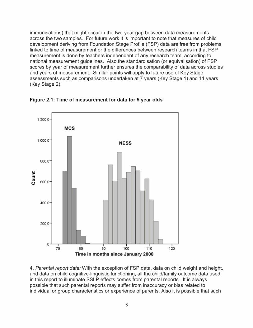
immunisations) that might occur in the two-year gap between data measurements across the two samples. For future work it is important to note that measures of child development deriving from Foundation Stage Profile (FSP) data are free from problems linked to time of measurement or the differences between research teams in that FSP measurement is done by teachers independent of any research team, according to national measurement guidelines. Also the standardisation (or equivalisation) of FSP scores by year of measurement further ensures the comparability of data across studies and years of measurement. Similar points will apply to future use of Key Stage assessments such as comparisons undertaken at 7 years (Key Stage 1) and 11 years (Key Stage 2).

Figure 2.1: Time of measurement for data for 5 year olds

4. Parental report data: With the exception of FSP data, data on child weight and height, and data on child cognitive-linguistic functioning, all the child/family outcome data used in this report to illuminate SSLP effects comes from parental reports. It is always possible that such parental reports may suffer from inaccuracy or bias related to individual or group characteristics or experience of parents. Also it is possible that such

8

problems may influence the results, although there is no obvious reason for such problems to affect one of the samples in this study more than the other.

5. Child cognitive and language development: When the NESS Impact Study was originally planned the intention was to investigate effects of SSLPs on children’s formally tested cognitive and language development at age 5, just as was done in earlier phases of the NESS Impact Study. And, in fact, at age 5 children in both NESS and MCS samples were administered select subscales of the British Ability Scales (BAS) (Elliot, Smith & McCulloch, 1996) to secure measurements of verbal and nonverbal abilities. However, inspection of the data from the two studies raised serious doubts about the equivalence of data across samples. The concern was that even though the BAS is normed so that there should be no average change from 3 to 5 years, in the MCS sample the degree of change proved to be approximately .5 standard deviations, which was implausibly large. It was concluded that this was a measurement artefact and unlikely to reflect real change in children’s average level of functioning. Hence BAS data were not used in subsequent MCS/NESS comparison analyses. Further details are in a note in Appendix C.

2.2 Design

SSLPs were a community-based initiative where everybody in the community was potentially a beneficiary of the programme. As in the original cross-sectional Impact Study (NESS, 2005a), an “intention to treat” design was adopted in the evaluation of the impact of SSLPs. Such an approach does not focus only on those children and families that have used SSLP services, but rather on all children and families living in SSLP areas. For the evaluation of SSLPs, this focus is appropriate because SSLPs had as their targets all children under five years of age in their area and their families. Thus 9-month old children and their families in SSLP areas were randomly sampled and followed up at 3 and 5 years of age, so that they could be compared with children and families similarly randomly sampled—by the MCS—but not residing in SSLP areas. It was decided that the MCS children to be used in such comparisons should live in areas that were as similar as possible to the SSLP areas. This decision was taken because the nature of an area was critical to it being allocated a SSLP. Hence this required matching areas where MCS children live with the SSLP areas in the NESS longitudinal study. The strategy and method by which this was achieved are described in the following section.

2.3 Identifying Potential Matched Areas

The areas where SSLPs were placed were chosen because of their particular characteristics. Because it was considered essential to select MCS children residing in areas as similar as possible to those in which the NESS Impact Study sample resided, a fundamental challenge was to identify small geographical areas that included a reasonable number of children participating in the MCS that could serve as comparison areas. Geographical analysis was used for this purpose (see Barnes et al., 2007; Frost

9

& Harper, 2007). The aim was to identify deprived areas containing MCS children/families that were as similar as possible to SSLP areas. Geographic Information Systems (GIS) were used to select potential areas and to extract data on them. The main indicator initially used to identify and select areas at this first stage was the overall score of the Index of Multiple Deprivation (IMD) 2004 (ODPM, 2004). The specification of areas was complicated by the fact that the original design of the MCS was based on sampling within 1998 electoral wards meaning that there was no direct comparability between the areas used in the MCS sampling and the areas for which IMD 2004 and Census information were available. To overcome this problem areas containing MCS children were identified using individual postcodes following strict guidelines specified by the ESRC longitudinal studies committee to prevent disclosure of personal information.

Initial tests were made using the IMD 2004 data to select wards that contained MCS children but did not overlap with any SSLP areas. These tests showed that the wards selected in this way were clearly less deprived than the SSLPs. Although some of them contained MCS children living in relatively deprived localities, the overall IMD scores for the wards reflected the fact that wards were large and contained both deprived and relatively non-deprived localities. It was necessary, therefore, to delineate potential comparator areas using the smaller, more focused, Super Output Areas (SOAs) so that relatively deprived localities could be defined more clearly. GIS were used to select SOAs within the same deprivation score range as SSLP areas. By using an intersection method, any SOA that overlapped with an SSLP area was excluded. Any area selected had to contain more than 9 children.

In order to enhance the comparability of SSLP and MCS areas we created a measure of the levels of affluence of the areas surrounding the MCS and SSLP areas, to serve as an indication of the neighbouring influence on an area and the degree to which it was an isolated area of deprivation. A rule-of-thumb 750 metre buffer was created around each area to represent typical walking distance. Postcodes within each buffer and for the internal areas were extracted and linked to income data (mean household annual income). From this, the following measures were calculated: (1) The ratio of the internal and external buffer weighted means for comparison between the two; (2) percent of households in the buffer whose mean household income was greater than the national average, thereby providing an indication of how affluent the surrounding population was; and (3) a measure of household income variation in the buffer zones. With these and IMD data in hand, it proved possible to identify 138 potential comparison areas that included MCS children/families, but did not have an SSLP.

2.4 Propensity Scoring

As already noted, propensity scoring (Rosenbaum & Rubin, 1983; Rubin, 1997; Pearl, 2009) can be used to estimate the contextual similarity to residing in an SSLP area based, in this case, on area (rather than individual) characteristics (Hill et al., 2005). We can then create “treatment” and “control” groups matched on their propensity to be a SSLP area. First, the probability of an area having a SSLP, its propensity score, was

10

estimated. This involved logistic regression, with the area’s status, SSLP vs. MCS, serving as the outcome to be predicted and several indices of area deprivation and other socio-demographic area characteristics used as predictors of area status (see Appendix A). This propensity score was used as a one-number summary of all the predictor variables for each area. The idea underlying matching on the propensity score is that if the two groups (SSLP and MCS) are balanced on all known area covariates, they are likely also to be matched on unknown and unmeasured covariates not included in the propensity analysis. Any imbalance across groups with respect to the confounding area covariates was used as a diagnostic of the adequacy of the propensity model and led to the creation of a refined propensity score and better balance. As long as important variables distinguishing between SSLP and MCS areas have not been omitted, the comparison of outcomes between SSLP and MCS groups should then have minimal bias due to the non-random allocation of SSLPs to areas.

In order to implement propensity scoring analysis, it was essential to determine which of the 138 aforementioned MCS areas were sufficiently comparable to the SSLP areas to be useful in an analysis. Therefore, the 138 identified MCS areas were compared with the 150 SSLP areas on 85 indices of deprivation and other area characteristics obtained from administrative sources (see Appendix A for more complete reporting of Propensity Scoring data, analysis and decision making).

SSLP populations were, in general, more disadvantaged than the comparison population drawn from the MCS sample. This posed problems in making comparisons between roughly equivalent NESS and MCS groups in order to evaluate putative SSLP effects. To deal with this, the NESS and MCS samples were each divided into five subgroups—or “strata”--reflecting the extent to which they were likely, on the basis of their area and demographic characteristics, to be chosen as an SSLP area. On the basis of such “propensity scoring”, areas in stratum 1 had the lowest propensity to be chosen as a SSLP area, basically because they had the least deprivation, and those in stratum 5 had the highest propensity to be chosen as a SSLP area, basically because they had the most deprivation. There proved to be only a single MCS area that qualified as having a high propensity (i.e., stratum 5) to be chosen as a SSLP area; this was due to the relative absence of very disadvantaged families and areas in the MCS data set. In the NESS sample, however, the reverse proved to be the case. Whereas 55 SSLP areas qualified for stratum 5 due to high levels of area and family deprivation, only two SSLP areas met criteria for having the lowest propensity to be chosen as a SSLP area (i.e., stratum 1) due to few SSLP areas being relatively advantaged economically and demographically. The differential distributions of MCS and SSLP areas across more and less disadvantaged areas and thus strata, displayed in Table 2.1, posed analytic challenges (see below).

11

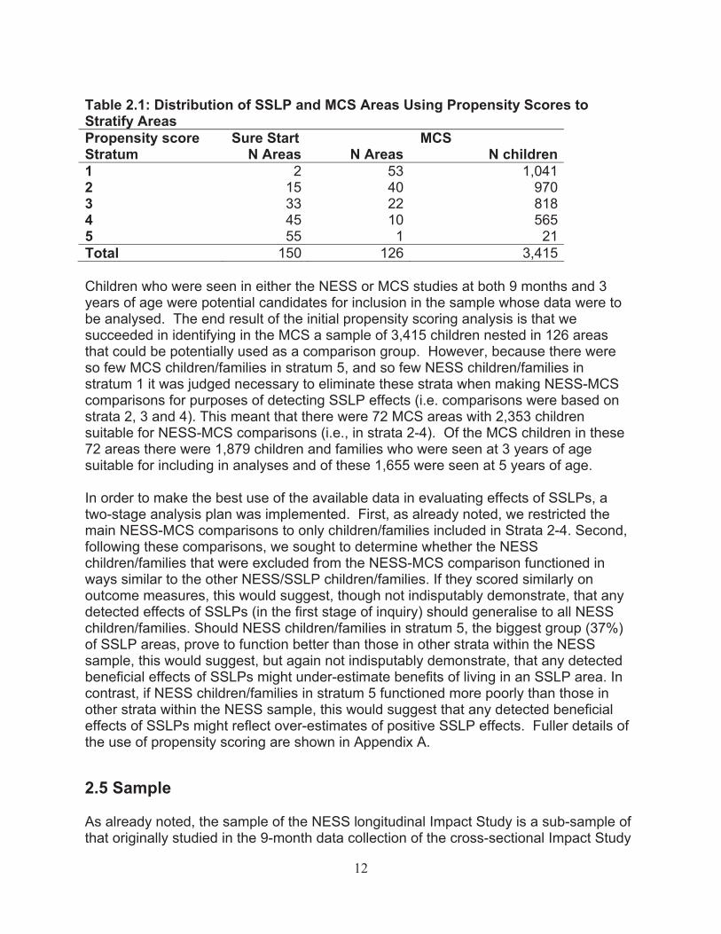
Table 2.1: Distribution of SSLP and MCS Areas Using Propensity Scores to Stratify Areas Propensity score Sure Start MCS Stratum N Areas N Areas N children 1 2 53 1,041 2 15 40 970 3 33 22 818 4 45 10 565 5 55 1 21 Total 150 126 3,415

Children who were seen in either the NESS or MCS studies at both 9 months and 3 years of age were potential candidates for inclusion in the sample whose data were to be analysed. The end result of the initial propensity scoring analysis is that we succeeded in identifying in the MCS a sample of 3,415 children nested in 126 areas that could be potentially used as a comparison group. However, because there were so few MCS children/families in stratum 5, and so few NESS children/families in stratum 1 it was judged necessary to eliminate these strata when making NESS-MCS comparisons for purposes of detecting SSLP effects (i.e. comparisons were based on strata 2, 3 and 4). This meant that there were 72 MCS areas with 2,353 children suitable for NESS-MCS comparisons (i.e., in strata 2-4). Of the MCS children in these 72 areas there were 1,879 children and families who were seen at 3 years of age suitable for including in analyses and of these 1,655 were seen at 5 years of age.

In order to make the best use of the available data in evaluating effects of SSLPs, a two-stage analysis plan was implemented. First, as already noted, we restricted the main NESS-MCS comparisons to only children/families included in Strata 2-4. Second, following these comparisons, we sought to determine whether the NESS children/families that were excluded from the NESS-MCS comparison functioned in ways similar to the other NESS/SSLP children/families. If they scored similarly on outcome measures, this would suggest, though not indisputably demonstrate, that any detected effects of SSLPs (in the first stage of inquiry) should generalise to all NESS children/families. Should NESS children/families in stratum 5, the biggest group (37%) of SSLP areas, prove to function better than those in other strata within the NESS sample, this would suggest, but again not indisputably demonstrate, that any detected beneficial effects of SSLPs might under-estimate benefits of living in an SSLP area. In contrast, if NESS children/families in stratum 5 functioned more poorly than those in other strata within the NESS sample, this would suggest that any detected beneficial effects of SSLPs might reflect over-estimates of positive SSLP effects. Fuller details of the use of propensity scoring are shown in Appendix A.

2.5 Sample

As already noted, the sample of the NESS longitudinal Impact Study is a sub-sample of that originally studied in the 9-month data collection of the cross-sectional Impact Study

12

(NESS, 2005a). Potential cross-sectional study participants living in 150 SSLP areas were identified with the assistance of the Child Benefit Office of (initially) the Department for Work and Pensions and (subsequently) HM Revenue and Customs. Potential cross-sectional study participants were randomly selected from the Child Benefit Register and a total of 12,575 9-month olds and their families were enrolled in the study, representing a response rate of 84.4%. The aim was to have at least 8,000 children/families in the longitudinal study when the children were 3 years of age. Of those seen at 9 months of age, 11,118 children/families from the 150 SSLP areas were randomly selected to be approached by a NESS fieldworker in order to collect data when the child was 3 years of age. Of these families 9,192 (82.7%) participated in the 3-year-old data collection. Of those not participating 388 refused (3.5%), 1,484 (13.3%) proved not to be contactable, often because they had moved and were untraceable; and 54 (0.5%) were not seen for diverse ’other’ reasons. Thus data collection was completed for 9,192 children and families when the children were 3 years of age. At 5 years of age 8000 of the children and families seen at 3 years of age were randomly selected to be followed-up. Of those approached, data was successfully collected on 7,258 children and families, representing a response rate of 91.6%. These children and families constitute the NESS longitudinal sample at 5 years of age.

The NESS children and families seen at 9 months but not seen at 5 years were compared with those seen on both occasions, separately for strata 1-5, on a range of demographic variables. Comparisons of those not seen at age five relative to those seen at both ages of measurements revealed that on several indicators families not re-studied were significantly less advantaged than those in strata 1-4, but significantly more advantaged than those in stratum 5 (i.e., for workless households, parent education and occupational status, poverty and ethnicity) (see Appendix B). Implications of these differences are considered in the results section 3.4.

MCS children/families were identified and recruited through a similar strategy by the MCS research team. As described earlier, 1,655 MCS children had been seen at 9 months, 3 and 5 years of age and were categorised in strata 2-4. This 5-year-old MCS sample represented a response rate of 88% of those seen at 3 years. These children came from areas that were matched—more or less—by means of propensity scoring to SSLP areas. In the MCS sample there were also children and families seen at 9 months but not at 5 years and they were compared on demographic characteristics to those seen on both occasions. The families not seen at 5 years were more likely to be from lone-parent and workless households and to be lower in occupational status, thereby appearing more deprived than the MCS subsample seen at both ages (see Appendix B for full comparisons). As described the decision was taken to test for differences between the NESS and MCS samples only within strata 2-4; thus, the final comparison samples at 5 years of age included 4,765 children/families in 93 SSLP areas and 1,655 children/families in 72 MCS areas.

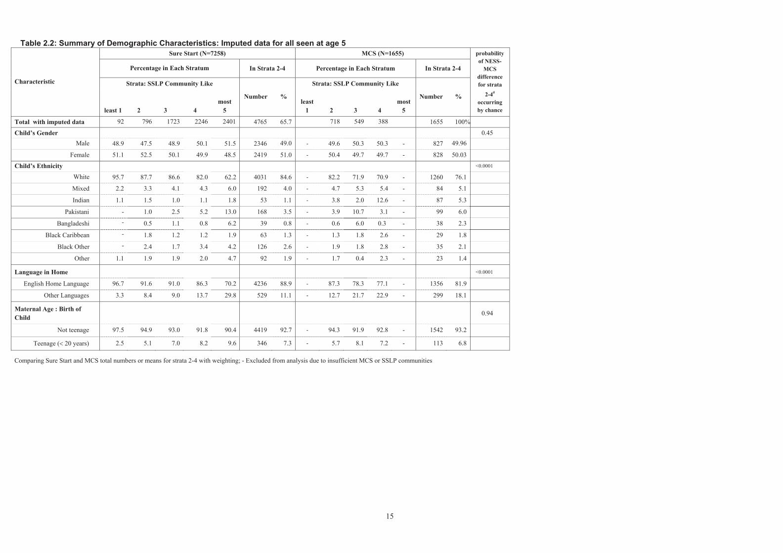
The demographic characteristics of the final NESS and MCS samples can be seen in Table 2.2. When strata 2-4 are considered, which are the strata used in NESS-MCS

13

comparisons, there are some demographic differences between the NESS and MCS samples. Some of these reveal greater disadvantage amongst the NESS sample (i.e., NESS had a higher proportion of lone parents, workless households, and respondents with lower levels of parental education), whereas other differences related to ethnicity suggest less disadvantage amongst the NESS sample (i.e., a higher proportion of white families and a lower proportion of homes where English was an additional language). On other background factors the two samples proved similar (i.e., proportion of mothers having given birth to the target child while under 20 years of age; proportion of households with total incomes below the poverty line). The areas in which NESS families resided also scored lower on the 2004 overall Index of Multiple Deprivation (data not shown).

14

acteristic difference

for strata

2-4#

occurring by chance le ast 1

Strata: SSLP Community Like

2 3 4 most

5

Number %

Strata: SSLP Community Like

lea st most 1 2 3 4 5

Number %

with imputed data 92 796 1723 2246 2401 4765 65.7 718 549 388 1655 % 100

’s Gender 0.45 Male 48.9 47.5 48.9 50.1 51.5 2346 49.0 - 49.6 50.3 50.3 - 827 49.96

Female 51.1 52.5 50.1 49.9 48.5 2419 51.0 - 50.4 49.7 49.7 - 828 50.03

Char

Sure Start (N=7258) MCS (N=1655) probability of NESS-

MCS Percentage in Each Stratum In Strata 2-4 Percentage in Each Stratum In Strata 2-4

Total

Child

Child’s Ethnicity <0.0001

White 95.7 87.7 86.6 82.0 62.2 4031 84.6 - 82.2 71.9 70.9 - 1260 76.1

Mixed 2.2 3.3 4.1 4.3 6.0 192 4.0 - 4.7 5.3 5.4 - 84 5.1

Indian 1.1 1.5 1.0 1.1 1.8 53 1.1 - 3.8 2.0 12.6 - 87 5.3

Pakistani - 1.0 2.5 5.2 13.0 168 3.5 - 3.9 10.7 3.1 - 99 6.0

Bangladeshi - 0.5 1.1 0.8 6.2 39 0.8 - 0.6 6.0 0.3 - 38 2.3

Black Caribbean - 1.8 1.2 1.2 1.9 63 1.3 - 1.3 1.8 2.6 - 29 1.8

Black Other - 2.4 1.7 3.4 4.2 126 2.6 - 1.9 1.8 2.8 - 35 2.1

Other 1.1 1.9 1.9 2.0 4.7 92 1.9 - 1.7 0.4 2.3 - 23 1.4

Language in Home <0.0001

English Home Language 96.7 91.6 91.0 86.3 70.2 4236 88.9 - 87.3 78.3 77.1 - 1356 81.9

Other Languages 3.3 8.4 9.0 13.7 29.8 529 11.1 - 12.7 21.7 22.9 - 299 18.1

Maternal Age : Birth of Child

0.94

Not teenage 97.5 94.9 93.0 91.8 90.4 4419 92.7 - 94.3 91.9 92.8 - 1542 93.2

Teenage (� 20 years) 2.5 5.1 7.0 8.2 9.6 346 7.3 - 5.7 8.1 7.2 - 113 6.8

Table 2.2: Summary of Demographic Characteristics: Imputed data for all seen at age 5

Comparing Sure Start and MCS total numbers or means for strata 2-4 with weighting; - Excluded from analysis due to insufficient MCS or SSLP communities

15

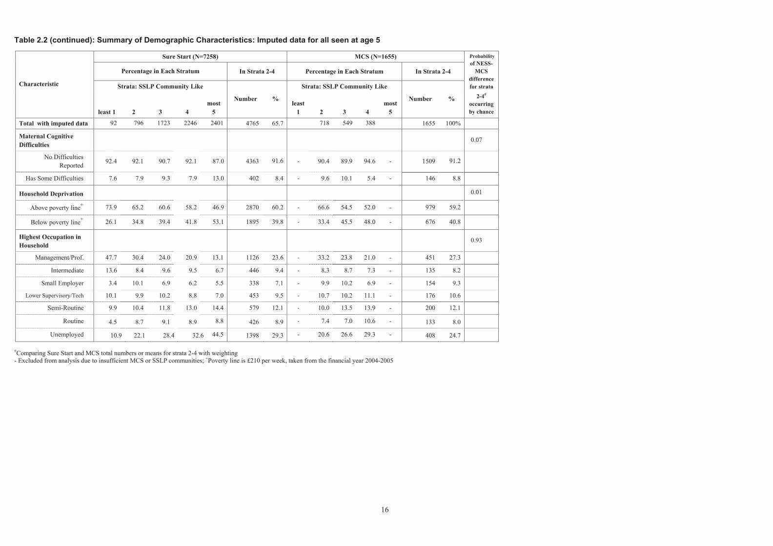
Table 2.2 (continued): Summary of Demographic Characteristics: Imputed data for all seen at age 5

Sure Start (N=7258) MCS (N=1655) Probability of NESS-

Percentage in Each Stratum In Strata 2-4 Percentage in Each Stratum In Strata 2-4 MCS

Characteristic difference for strata

2-4#

occurring by chance

Strata: SSLP Community Like

most least 1 2 3 4 5

Number %

Strata: SSLP Community Like

least most 1 2 3 4 5

Number %

Total with imputed data 92 796 1723 2246 2401 4765 65.7 71 548 389 8 1655 100%

Maternal Cognitive Difficulties

0.07

No Difficulties Reported

92.4 92.1 90.7 92.1 87.0 4363 91.6 - 90.4 89.9 94.6 - 1509 91.2

Has Some Difficulties 7.6 7.9 9.3 7.9 13.0 402 8.4 - 9.6 10.1 5.4 - 146 8.8

Household Deprivation

Above poverty line+

Below poverty line+

73.9 65.2 60.6 58.2 46.9

26.1 34.8 39.4 41.8 53.1

2870 60.2

1895 39.8

- 66.6 54.5 52.0 -

- 33.4 45.5 48.0 -

979 59.2

676 40.8

0.01

Highest Occupation in Household

0. 93

Management/Prof. 47.7 30.4 24.0 20.9 13.1 1126 23.6 - 33.2 23.8 21.0 - 451 27.3

Intermediate 13.6 8.4 9.6 9.5 6.7 446 9.4 - 8.3 8.7 7.3 - 135 8.2

Small Employer 3.4 10.1 6.9 6.2 5.5 338 7.1 - 9.9 10.2 6.9 - 154 9.3

Lower Supervisory/Tech 10.1 9.9 10.2 8.8 7.0 453 9.5 - 10.7 10.2 11.1 - 176 10.6

Semi-Routine 9.9 10.4 11.8 13.0 14.4 579 12.1 - 10.0 13.5 13.9 - 200 12.1

Routine 4.5 8.7 9.1 8.9 8.8 426 8.9 - 7.4 7.0 10.6 - 133 8.0

Unemployed 10.9 22.1 28.4 32.6 44.5 1398 29.3 - 20.6 26.6 29.3 - 408 24.7

#Comparing Sure Start and MCS total numbers or means for strata 2-4 with weighting - Excluded from analysis due to insufficient MCS or SSLP communities; +Poverty line is £210 per week, taken from the financial year 2004-2005

16

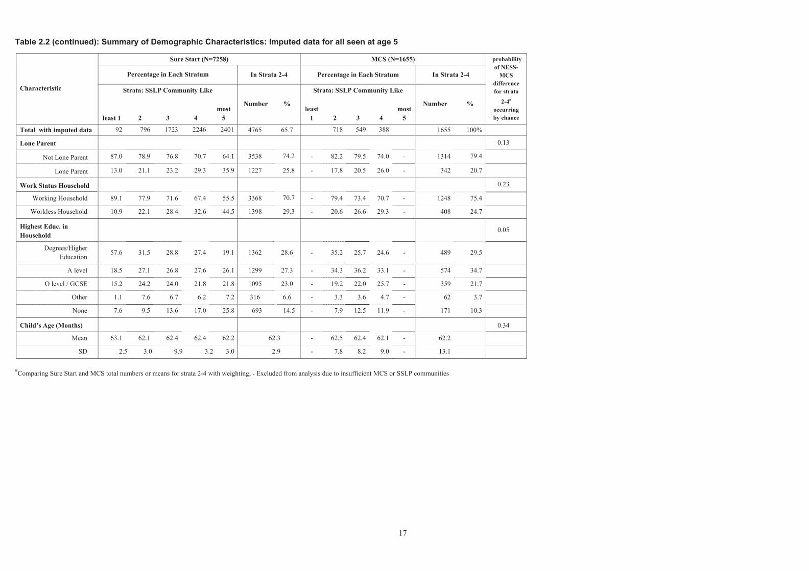
Table 2.2 (continued): Summary of Demographic Characteristics: Imputed data for all seen at age 5

Sure Start (N=7258) MCS (N=1655) probability of NESS-

Percentage in Each Stratum In Strata 2-4 Percentage in Each Stratum In Strata 2-4 MCS

Characteristic difference for strata

2-4#

occurring by chance

Strata: SSLP Community Like

least 1 2 3 4 most

5

Number %

Strata: SSLP Community Like

least 1 2 3 4

most 5

Number %

Total with imputed data 92 796 1723 2246 2401 4765 65.7 718 549 388 1655 100%

Lone Parent 0.13

Not Lone Parent 87.0 78.9 76.8 70.7 64.1 3538 74.2 - 82.2 79.5 74.0 - 1314 79.4

Lone Parent 13.0 21.1 23.2 29.3 35.9 1227 25.8 - 17.8 20.5 26.0 - 342 20.7

Work Status Household

Working Household

Workless Household

89.1 77.9 71.6 67.4 55.5

10.9 22.1 28.4 32.6 44.5

3368 70.7

1398 29.3

- 79.4 73.4 70.7 -

- 20.6 26.6 29.3 -

1248 75.4

408 24.7

0.23

Highest Educ. in Household

0.05

Degrees/Higher Education

57.6 31.5 28.8 27.4 19.1 1362 28.6 - 35.2 25.7 24.6 - 489 29.5

A level 18.5 27.1 26.8 27.6 26.1 1299 27.3 - 34.3 36.2 33.1 - 574 34.7

O level / GCSE 15.2 24.2 24.0 21.8 21.8 1095 23.0 - 19.2 22.0 25.7 - 359 21.7

Other 1.1 7.6 6.7 6.2 7.2 316 6.6 - 3.3 3.6 4.7 - 62 3.7

None 7.6 9.5 13.6 17.0 25.8 693 14.5 - 7.9 12.5 11.9 - 171 10.3

Child’s Age (Months) 0.34

Mean 63.1 62.1 62.4 62.4 62.2 62.3 - 62.5 62.4 62.1 - 62.2

SD 2.5 3.0 9.9 3.2 3.0 2.9 - 7.8 8.2 9.0 - 13.1

#Comparing Sure Start and MCS total numbers or means for strata 2-4 with weighting; - Excluded from analysis due to insufficient MCS or SSLP communities

17

2.6 Data Collection

The families participating in the NESS longitudinal Impact Study, the “Study of Children, Families & Services in the Community”, provided extensive information on child and family functioning during the course of a single home visit conducted by a specially trained fieldworker, typically lasting around 90 minutes when children were 9 months of age and then again at 3 and 5 years of age. In the case of home visits to families with 9-month-olds, a survey research workforce under subcontract from the Office of National Statistics carried out data collection. Home visits to families with 3-year-olds and 5-year-olds, that involved child assessments as well as parental interviews, were carried out by a field force especially hired and trained for this purpose by the Institute for the Study of Children, Families and Social Issues, Birkbeck University of London (which houses NESS). MCS data were gathered by similar means by survey research businesses contracted by the MCS team at the Institute of Education.

During home visits, several sets of data were gathered in order to assess the effects of SSLPs on child development and family functioning. In addition to these dependent-variable outcome measures, demographic and background information were collected from each family, as well as area characteristics on each community, to serve principally as control variables in the analyses to be presented. Additionally, data on children’s Foundation Stage Profiles were obtained from the then Department for Children, Schools and Families. The reason for including them, fundamentally, was because they provided a picture of the child’s school functioning from a teacher. Teachers differ from parents who supplied other data on child and family functioning in that they have typically been exposed to lots of children, and will have a wider basis for comparison. Thus, there are grounds for suspecting that teacher evaluations could be more objective and thus informative than parent reports.

The Foundation Stage Profile (FSP) records the child’s achievement as reported by their teacher at the end of the first year of school for children in state schools in England. The assessments are made on the basis of the accumulated observations and knowledge of the whole child. A handbook for teachers describing the criteria to be used in the FSP is available at: http://nationalstrategies.standards.dcsf.gov.uk/node/113520.

The FSP covers six areas of learning, covering children’s physical, intellectual, emotional and social development. The first 3 areas are made up of several subscales, and the last 3 areas have only one rating scale. 1. Personal, Social and Emotional Development (PSE):

x Dispositions and Attitudes x Social Development x Emotional Development

2. Communication, Language and Literacy (CLL): x Language for Communication and Thinking

18

x Linking Sounds and Letters x Reading x Writing

3. Problem-solving, Reasoning and Numeracy (Mathematical development) (MAT): x Numbers as Labels for Counting x Calculating x Shape, Space and Measures

4. Knowledge and Understanding of the World (KUW) 5. Physical Development (PD) 6. Creative Development (CD)

Each assessment scale is rated 0-9 as follows:

x 0 points – assigned to a child for whom it has not been possible to record an assessment, because of the nature of their individual needs, at this stage of their development.

x 1-3 points (‘Stepping Stones’) – these describe a child who is still progressing towards the achievements described in the Early Learning Goals. Most children will achieve all of these 3 points before achieving any of the Early Learning Goals, but there may be exceptions to this pattern. A child who does not score on any of these stepping stones is experiencing significant developmental delay.

x 4-8 points (Early Learning Goals) – these are drawn from the Early Learning Goals themselves, presented in order of difficultly, according to evidence from trials. However, the points are not necessarily hierarchical and a child may achieve a later point without having achieved some or all of the earlier points.

x 9 points – this describes a child who has received all the points from 1-8 on that scale, has developed further in both depth and breadth and is working consistently beyond the level of the Early Learning Goals.

Children who achieve a scale score of 6 points or more for any assessment scale are classified as working securely within the Early Learning Goals for that assessment scale. They are deemed to have achieved a good level of development by the end of the foundation stage.

If a child achieves a total score of 78 points or more across all 13 assessment scales then they will have achieved an average of 6 points per scale (although in practice could have scored higher or lower than this for each scale). When a child who achieves an overall score of 78 points, alongside a score of 6 or more in each of the PSE and CLL scales, then the child is deemed to be reaching a good level of development.

Foundation Stage Profile data show changes over time, even across the two-year period which separates when teachers evaluated children participating in the MCS and the NESS data collections. For example, for national data, comparing 2009 with 2008 3% more children were scoring 6 points or more (“working securely”) in Communication, Language and Literacy; and similar changes can be found across FSP scales for other years (DCSF, 2009). A consequence of such year-by-year changes

19

is that any NESS vs. MCS comparison would be potentially compromised by year of measurement effects. In order to overcome the complicating fact that the proportion of children obtaining higher grades can change from year to year we have used national data on all children in England to create within-year standardised scores for every child, so that the relative ranking of MCS children in one year can be compared with those in the NESS sample assessed in a different year. This strategy eliminates the effect of any year-by-year changes within FSP data, and provides a fair basis for comparison across samples and across years. FSP data has the advantage that it is clearly measured in a way that is the same for both MCS and NESS studies and that is completely independent of different research team behaviours or the decision to implement Sure Start in an area.

The measures delineated below and used in analyses reflect those variables where the procedures within the NESS and MCS studies were sufficiently similar to be comparable across the studies.

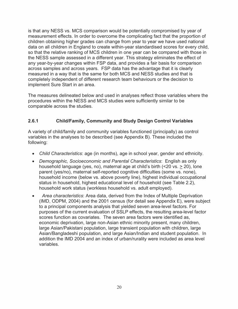
2.6.1 Child/Family, Community and Study Design Control Variables

A variety of child/family and community variables functioned (principally) as control variables in the analyses to be described (see Appendix B). These included the following:

x Child Characteristics: age (in months), age in school year, gender and ethnicity. x Demographic, Socioeconomic and Parental Characteristics: English as only

household language (yes, no), maternal age at child’s birth (<20 vs. > 20), lone parent (yes/no), maternal self-reported cognitive difficulties (some vs. none), household income (below vs. above poverty line), highest individual occupational status in household, highest educational level of household (see Table 2.2), household work status (workless household vs. adult employed).

x Area characteristics: Area data, derived from the Index of Multiple Deprivation (IMD, ODPM, 2004) and the 2001 census (for detail see Appendix E), were subject to a principal components analysis that yielded seven area-level factors. For purposes of the current evaluation of SSLP effects, the resulting area-level factor scores function as covariates. The seven area factors were identified as, economic deprivation, large non-Asian ethnic minority present, many children, large Asian/Pakistani population, large transient population with children, large Asian/Bangladeshi population, and large Asian/Indian and student population. In addition the IMD 2004 and an index of urban/rurality were included as area level variables.

20

2.6.2 Child/Family Dependent/Outcome Variables

The outcome variables for children and families at the 5-year contact and used in analyses are summarised below, with further detail in Appendix C:

Child Educational Development: Foundation Stage Profile (FSP):

1. Personal, Social and Emotional Development (PSE): 2. Communication, Language and Literacy (CLL): 3. Problem-solving, Reasoning and Numeracy (MAT): 4. Knowledge and Understanding of the World (KUW) 5. Physical Development (PD) 6. Creative Development (CD) 7. Total FSP score

Child social and emotional development: emotional dysregulation, positive social behaviour, internalising behaviour, self-regulation. These were all obtained by means of parental report.

Child Physical Health: general physical health based on detailed reports by parents of the child’s health history; and body mass index (BMI), based upon height and weight measurements by a researcher.

Parenting and Family Functioning: harsh discipline, home chaos, home learning environment (HLE), and parent’s involvement with school (all parent report).

Maternal well-being: life satisfaction; depression Local Area: perceived area safety, rated by mother. Parental Employment change: The likelihood of change in working/workless household status from when the child was 9 months of age to when the child is five years of age is examined. – Note this is included in our section on change in outcomes and has a different form of analysis to other outcomes in that change since the child was 9 months old is estimated.

21

3. RESULTS

Four stages of analysis are presented: 1. Addresses the issue of whether there were across-the-board effects of SSLPs on

child and family functioning when children were 5 years of age or in terms of change over time in the case of outcomes measured at both 3 and 5 years of age.

2. Seeks to determine whether any effects detected by comparing NESS and MCS comparison samples in Strata 2-4 may have under, over or accurately estimated overall effects of SSLPs.

3. Focuses upon whether detected effects of SSLPs varied across demographically-defined sub-populations (e.g., workless households, lone-parent families).

4. Assesses whether attrition might undermine confidence in any results emerging from the prior analysis.

Critically important to appreciate is that all analyses outlined in this section were carried out three times:

1. using only those cases for which there was no missing data at age 5; 2. using all cases seen at age 5, with any missing data imputed multiple times before

being subject to analysis (N=7,258 for NESS, 1,655 for MCS); and 3. using all cases seen at age 3 irrespective of whether they were seen at age 5,

again with missing data imputed multiple times before being subject to analysis (N=9,192 for NESS, 1,879 for MCS).

Missing values on all independent and dependent variables were estimated based on standard multiple-imputation procedures in the second two sets of analyses (Rubin, 1987). The imputation approach represents an attempt to counteract the possibility that cases with missing data differ in some way from cases with complete data and the biasing effects that their exclusion from the analysis could have on the results. Ten imputed data sets were created (for each of the two sets of imputation-related analyses), which ensured that all model estimates will be over 90% efficient. For more detail of the imputation procedure see Appendix D. Only significant differences between SSLP and comparison areas that emerged in all three sets of analyses are regarded as reliable and meaningful and thus presented and interpreted in this report. This conservative procedure for discerning SSLP effects maximises confidence in the results. While in the main text only tables showing results which proved significant across all three sets of analyses are presented, parallel tables pertaining to each individual set of results are presented in Appendix F.

3.1 First stage: Overall (across-the-board) Effects of SSLPs

The first stage of data analysis was designed to assess the main (or across-the-board) effects of SSLPs on each dependent variable, after taking into account pre-existing differences between SSLP and comparison families and communities in their demographic characteristics (shown in Table 2.2). Thus, an overall main effect involves

22

a significant difference between SSLP and comparison communities on an outcome without taking into consideration the possibility that subpopulations might be differentially affected by SSLPs. In other words, it addresses the question as to whether, on average across all types of children and families, effects of SSLPs emerged. (Recall that these across-the-board comparisons do not involve the entire NESS sample, but only those areas in strata 2-4, the ones most similar across NESS and MCS samples). Recall as well that whereas virtually no sub-population-specific SSLP effects emerged in the second phase of inquiry (when the children were 3 years old); they were very much present in the first stage of impact analysis. Caution is required in interpreting main effect findings because these can be importantly qualified by interactions involving sub-populations.

In order to determine whether main effects of SSLPs on child development and family functioning were detectable, the data were analysed using multilevel models, which take into account the hierarchical structure of the data, with children and families nested within communities, some of which are SSLP communities and some comparison communities. Linear models are used for the continuous measures and logistic models for binary outcomes. Summary statistics (i.e. means, standard deviations) for the NESS-MCS comparisons using imputed data for all cases seen at 5 years, are presented for each of the outcomes in Table 3.1. The overall results of SSLP vs. MCS comparisons for the analyses (i.e. estimated effects) can be seen in Table 3.2. The effect sizes listed in Table 3.2 are the average of effects sizes across all three sets of analyses, in terms of differences between groups measured in standard deviation units. Effect sizes are a way of representing the magnitude of effects in a way that allows comparison between different variables regardless of their scale of measurement. It also affords a convenient way of comparing effects detected in the evaluation of one intervention project with those of another.

We use statistical significance as an indication of the confidence that we can have that the finding is genuine. However, the fact that a given finding is statistically significant does not necessarily mean that it is important. A finding of a small difference between two conditions may well be statistically significant but may be trivial, particularly if it applies to only a small group. Therefore a measure of the size of the difference is crucial. Effect size is the name given to a number of statistical measures of the magnitude of a difference, whether over time within the same group or between groups. The most commonly employed measure of effect size used is the difference between two scores divided by the standard deviation. In comparing NESS and MCS samples the effect size was calculated by dividing the NESS-MCS difference in scores by the standard deviation of the total sample. In studies using RCTs (e.g. drug trials) effect sizes of around 0.2 are usually regarded as ‘small’, of 0.5 as ‘medium’ and 0.8 or greater as ‘large’. However the importance for policy of a particular effect size is also related to the proportion of the population effected, and the effects associated with factors linked to policy are typically in the “small” range, e.g., the effect size for eligibility for free school meals (FSM) is 0.23 for literacy and 0.15 for numeracy (Key Stage 2 results, Sammons et al., 2008). Where population-scale differences are involved smaller effect sizes may well be of policy significance. For example a population-wide

23

change for IQ with an effect size as small as 0.1 would have profound implications for education and the economy.

After taking into consideration pre-existing family and area background characteristics (in all sets of analyses), the three sets of analyses comparing children and families living in SSLP areas and those living in similar areas not receiving SSLPs revealed six positive and two negative effects of SSLPs and numerous non-effects with respect to child and family functioning when children were 5 years old:

For children x children growing up in SSLP areas had lower BMIs than children growing up in

non-SSLP areas. This was not due to their being less likely to be obese, but to their being less likely to be overweight (i.e., criteria for overweight and obesity are different).

x Children growing up in SSLP areas were reported to have better physical health

Turning to apparently positive effects of SSLPs on maternal well being and family functioning, in comparison to mothers in non-SSLP areas, mothers residing in SSLP areas reported: x providing a more cognitively stimulating home learning environment. x providing a less chaotic home environment for their children , x greater life satisfaction, x engaging in less harsh discipline of their children,

On the negative side, however, compared to those in non-SSLP areas: x mothers in SSLP areas reported more depressive symptoms and x parents in SSLP areas were less likely to visit their child’s school for

parent/teacher meetings or other arranged visits. Although the overall incidence of such visits was low generally.

Finally, no differences emerged between the NESS and MCS groups on 7 measures of cognitive and social development from the Foundation Stage Profile completed by teachers, 4 measures of socio-emotional development based on mothers’ ratings, and mothers’ ratings of area safety.

In summary, across a total of 21 outcomes3 evaluated, significant effects of SSLPs emerged in the case of 8 outcomes. The estimated SSLP effects are displayed in Table 3.2 for the results emanating from the analysis of imputed data for all cases seen at 5 years. The data in the table chronicle the degree of difference, including confidence intervals, between SSLP and MCS areas, after adjusting for child and family background factors and community characteristics, on measurements made at age 5 (shown in Table 2.2). Positive values on the mean difference scores indicate that SSLP areas scored higher than the comparison areas, as do odds ratios greater than 1.00; negative values of mean difference scores indicate the opposite, as do odds ratios less

3 Definitions of the outcomes can be found in Appendix C.

24

than 1.00. The effects of the strata, demographic, family characteristics and area level measures are shown in Appendix F.

Although Table 3.2 presents the main effects of SSLPs, that is, whether the SSLP and comparison samples differed significantly across the entire sample, net of control variables, on age 5 measurements, these results do not indicate whether effects of SSLPs varied for specific subgroups related to gender, ethnicity, or income. Such interaction effects are reported in the third major stage of analysis. It is possible that an apparently negative, or positive or null result does not accurately reflect the situation— due to subsequent qualification by an interaction effect; caution is therefore warranted in drawing conclusions on the basis of these main-effect results alone. An interaction effect would indicate that the effect of exposure to SSLPs was not the same across different subgroups. One might discover, for instance, that SSLPs affected the parenting of lone parents more than partnered parents.

25

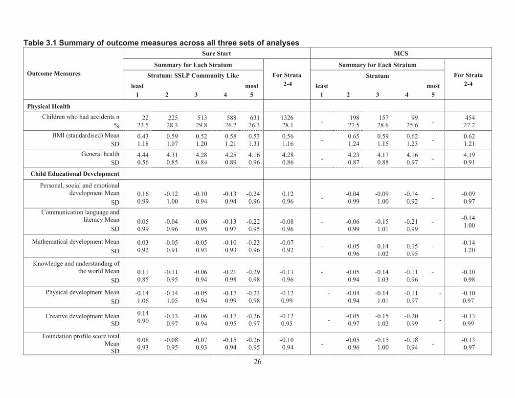
Table 3.1 Summary of outcome measures across all three sets of analyses

Outcome Measures

Sure Start MCS

Summary for Each Stratum For Strata

2-4

Summary for Each Stratum For Strata

2-4 Stratum: SSLP Community Like

least 1 2 3 4

most 5

Stratum least

1 2 3 4 most

5

Physical Health Children who had accidents n 22 225 513 588 631 1326 - 198 157 99 - 454

% 23.5 28.3 29.8 26.2 26.3 28.1 27.5 28.6 25.6 27.2 BMI (standardised) Mean 0.43 0.59 0.52 0.58 0.53 0.56 - 0.65 0.59 0.62 - 0.62

SD 1.18 1.07 1.20 1.21 1.31 1.16 1.24 1.15 1.23 1.21 General health 4.44 4.31 4.28 4.25 4.16 4.28 - 4.23 4.17 4.16 - 4.19

SD

Child Educational Development

0.56 0.85 0.84 0.89 0.96 0.86 0.87 0.88 0.97 0.91

Personal, social and emotional development Mean 0.16 -0.12 -0.10 -0.13 -0.24 0.12 - -0.04 -0.09 -0.14 - -0.09

SD 0.99 1.00 0.94 0.94 0.96 0.96 0.99 1.00 0.92 0.97 Communication language and

literacy Mean SD

0.05 0.99

-0.04 0.96

-0.06 0.95

-0.13 0.97

-0.22 0.95

-0.08 0.96

- -0.06 0.99

-0.15 1.01

-0.21 0.99

- -0.14 1.00

Mathematical development Mean SD

0.03 0.92

-0.05 0.91

-0.05 0.93

-0.10 0.93

-0.23 0.96

-0.07 0.92 - -0.05

0.96 -0.14 1.02

-0.15 0.95

- -0.14 1.20

Knowledge and understanding of the world Mean 0.11 -0.11 -0.06 -0.21 -0.29 -0.13 - -0.05 -0.14 -0.11 - -0.10

SD 0.85 0.95 0.94 0.98 0.98 0.96 0.94 1.03 0.96 0.98

Physical development Mean -0.14 -0.14 -0.05 -0.17 -0.23 -0.12 - -0.04 -0.14 -0.11 - -0.10 SD 1.06 1.05 0.94 0.99 0.98 0.99 0.94 1.01 0.97 0.97

Creative development Mean SD

0.14 0.90

-0.13 0.97

-0.06 0.94

-0.17 0.95

-0.26 0.97

-0.12 0.95 - -0.05

0.97 -0.15 1.02

-0.20 0.99 - -0.13

0.99

Foundation profile score total Mean

SD

0.08 0.93

-0.08 0.95

-0.07 0.93

-0.15 0.94

-0.26 0.95

-0.10 0.94 - -0.05

0.96 -0.15 1.00

-0.18 0.94 - -0.13

0.97

26

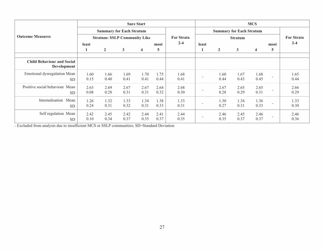
Outcome Measures

Sure Start MCS

Summary for Each Stratum For Strata

2-4

Summary for Each Stratum For Strata

2-4 Stratum: SSLP Community Like

least 1 2 3 4

most 5

least 1

Stratum

2 3 4 most

5

Child Behaviour and Social Development

Emotional dysregulation Mean 1.60 1.66 1.69 1.70 1.75 1.68 - 1.60 1.67 1.68 - 1.65 SD 0.15 0.40 0.41 0.41 0.44 0.41 0.44 0.43 0.45 0.44

Positive social behaviour Mean 2.63 2.69 2.67 2.67 2.64 2.68 - 2.67 2.65 2.65 - 2.66 SD 0.08 0.28 0.31 0.31 0.32 0.30 0.28 0.29 0.31 0.29

Internalisation Mean 1.26 1.32 1.33 1.34 1.38 1.33 - 1.30 1.34 1.36 - 1.33 SD 0.24 0.31 0.32 0.31 0.33 0.31 0.27 0.31 0.33 0.30

Self regulation Mean SD

2.42 0.10

2.45 0.34

2.42 0.37

2.44 0.35

2.41 0.37

2.44 0.35 - 2.46

0.35 2.45 0.37

2.46 0.37 - 2.46

0.36

- Excluded from analysis due to insufficient MCS or SSLP communities; SD=Standard Deviation

27

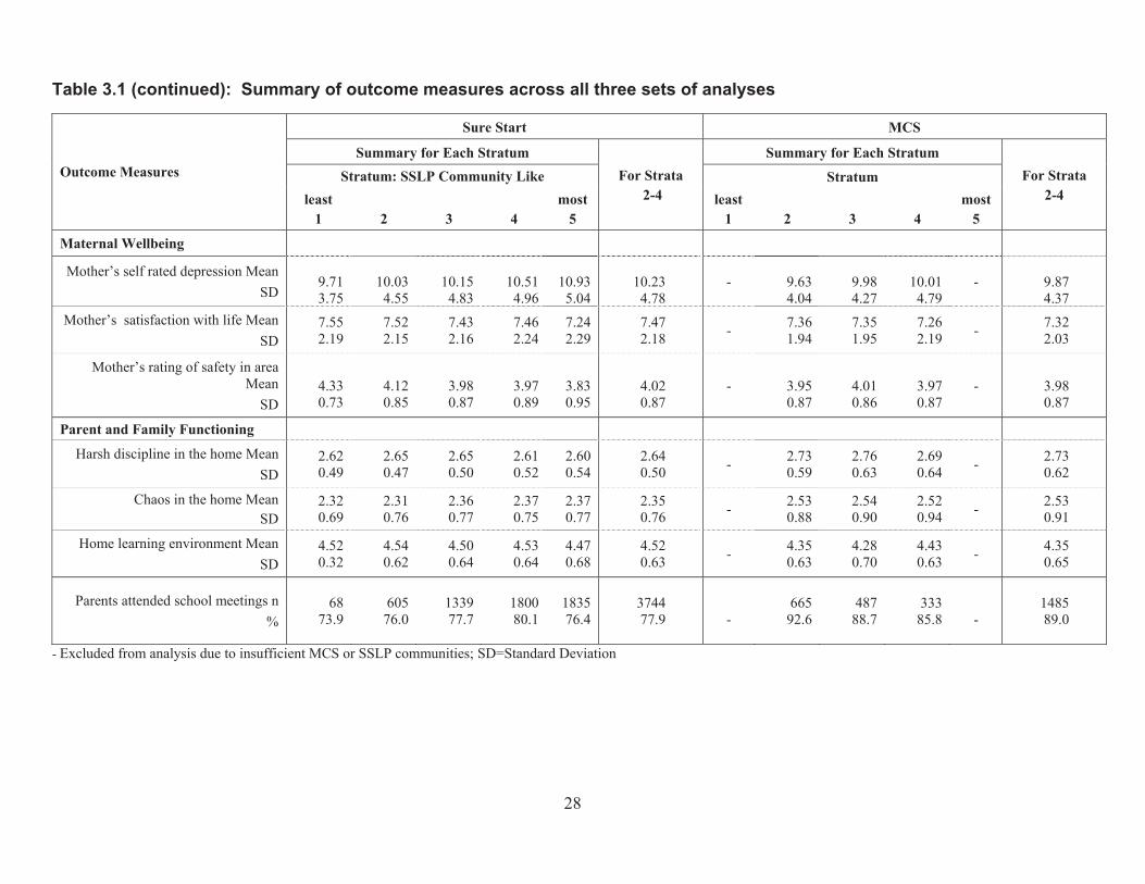
Outcome Measures

Sure Start MCS

Summary for Each Stratum For Strata

2-4

Summary for Each Stratum For Strata

2-4 Stratum: SSLP Community Like

least 1 2 3 4

most 5

Stratum least

1 2 3 4 most

5

Maternal Wellbeing

Mother’s self rated depression Mean SD

9.71 3.75

10.03 4.55

10.15 4.83

10.51 4.96

10.93 5.04

10.23 4.78

- 9.63 4.04

9.98 4.27

10.01 4.79

- 9.87 4.37

Mother’s satisfaction with life Mean 7.55 7.52 7.43 7.46 7.24 7.47 - 7.36 7.35 7.26 - 7.32 SD

Mother’s rating of safety in area

2.19 2.15 2.16 2.24 2.29 2.18 1.94 1.95 2.19 2.03

Mean 4.33 4.12 3.98 3.97 3.83 4.02 - 3.95 4.01 3.97 - 3.98 SD 0.73 0.85 0.87 0.89 0.95 0.87 0.87 0.86 0.87 0.87

Parent and Family Functioning

Harsh discipline in the home Mean 2.62 2.65 2.65 2.61 2.60 2.64 - 2.73 2.76 2.69 - 2.73 SD 0.49 0.47 0.50 0.52 0.54 0.50 0.59 0.63 0.64 0.62

Chaos in the home Mean 2.32 2.31 2.36 2.37 2.37 2.35 - 2.53 2.54 2.52 - 2.53 SD 0.69 0.76 0.77 0.75 0.77 0.76 0.88 0.90 0.94 0.91

Home learning environment Mean 4.52 4.54 4.50 4.53 4.47 4.52 - 4.35 4.28 4.43 - 4.35 SD 0.32 0.62 0.64 0.64 0.68 0.63 0.63 0.70 0.63 0.65

Parents attended school meetings n 68 605 1339 1800 1835 3744 665 487 333 1485 % 73.9 76.0 77.7 80.1 76.4 77.9 - 92.6 88.7 85.8 - 89.0

Table 3.1 (continued): Summary of outcome measures across all three sets of analyses

- Excluded from analysis due to insufficient MCS or SSLP communities; SD=Standard Deviation

28

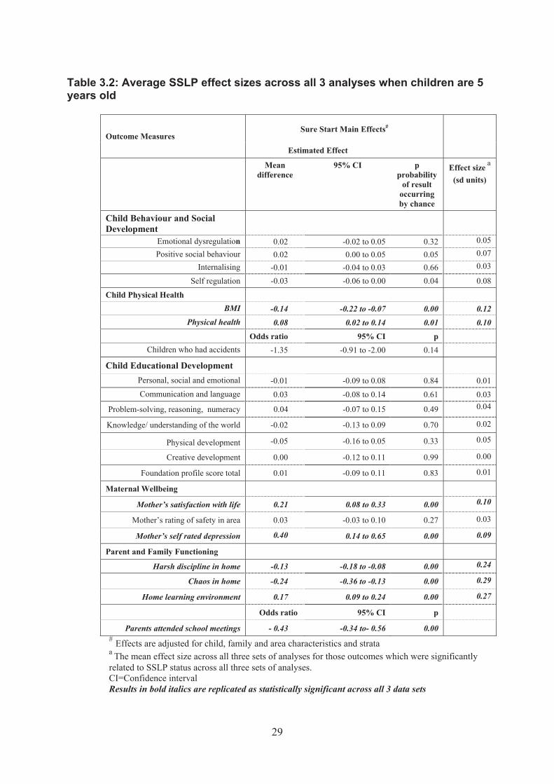
Table 3.2: Average SSLP effect sizes across all 3 analyses when children are 5 years old

Outcome Measures Sure Start Main Effects#

Estimated Effect

Mean difference

95% CI p probability

of result occurring by chance

Effect size a

(sd units)

Child Behaviour and Social Development

Emotional dysregulation 0.02 -0.02 to 0.05 0.32 0.05

Positive social behaviour 0.02 0.00 to 0.05 0.05 0.07

Internalising -0.01 -0.04 to 0.03 0.66 0.03

Self regulation -0.03 -0.06 to 0.00 0.04 0.08

Child Physical Health BMI -0.14 -0.22 to -0.07 0.00 0.12

Physical health

Children who had accidents

0.08 0.02 to 0.14 0.01 Odds ratio 95% CI p

-1.35 -0.91 to -2.00 0.14

0.10

Child Educational Development Personal, social and emotional -0.01 -0.09 to 0.08 0.84 0.01 Communication and language 0.03 -0.08 to 0.14 0.61 0.03

Problem-solving, reasoning, numeracy 0.04 -0.07 to 0.15 0.49 0.04

Knowledge/ understanding of the world -0.02 -0.13 to 0.09 0.70 0.02

Physical development

Creative development

Foundation profile score total

-0.05 -0.16 to 0.05 0.33

0.00 -0.12 to 0.11 0.99

0.01 -0.09 to 0.11 0.83

0.05

0.00

0.01

Maternal Wellbeing

Mother’s satisfaction with life 0.21 0.08 to 0.33 0.00 0.10

Mother’s rating of safety in area 0.03 -0.03 to 0.10 0.27 0.03

Mother’s self rated depression 0.40 0.14 to 0.65 0.00 0.09

Parent and Family Functioning

Harsh discipline in home -0.13 -0.18 to -0.08 0.00 0.24

Chaos in home -0.24 -0.36 to -0.13 0.00 0.29

Home learning environment

Parents attended school meetings

0.17 0.09 to 0.24 0.00

Odds ratio 95% CI p

- 0.43 -0.34 to- 0.56 0.00

0.27

# Effects are adjusted for child, family and area characteristics and strata a The mean effect size across all three sets of analyses for those outcomes which were significantly related to SSLP status across all three sets of analyses. CI=Confidence interval Results in bold italics are replicated as statistically significant across all 3 data sets

29

Change from 3 to 5 years: Because some of the dependent measures included in the analyses just described were also measured in identical or nearly-identical fashion at the 3-year assessment, it proved possible to evaluate the effects of SSLPs on change in functioning from 3 to 5 years of age. This was accomplished by rerunning the same statistical models used to produce the results just summarised, with one minor modification: the 3-year version of the 5-year outcome to be predicted was added to the model as a covariate, thereby changing the outcome from a measure of functioning at 5 years of age to one of change from 3 to 5 years. The exception to this concerns change in workless household status, which is considered as change since the child was 9 months old. Results of this analysis are presented in Table 3.3. The effect sizes quoted in Table 3.3 are the average of effects sizes across all three sets of analyses.

Inspection of the table reveals that of 11 repeatedly measured dependent variables, 5 showed evidence of SSLP effects on change over time in child or parent functioning in all three sets of analyses.

In comparison with those in non-SSLP areas, mothers in SSLP areas: x Showed more positive change (i.e., greater increase) in life satisfaction, x Reported more positive change in the home learning environment (i.e.,

greater improvement), x Reported more positive change in harsh discipline (i.e., greater decrease).

In addition: x There was a greater decrease in workless household status (from 9 months to

5 years of age) for families in SSLP areas

Children in SSLP areas, however: x manifested less positive change in self regulation, that is, their capacity to

control or manage their actions. This, however, appeared to be due to the fact that the children in the SSLP areas manifested greater self regulation at age 3, but by the time of the age-5 follow up, the MCS comparison group of children had caught up with them. This resulted in there being no difference in self regulation between the two groups by the time children were 5.

There were no differences associated with SSLPs on change from age 3 to 5 years in child emotional dysregulation, positive social behaviour or internalising behaviour as rated by parents; no differences in child accidents, mother’s depression, or chaotic home environments (see Appendix C for explanation of the measures).

30

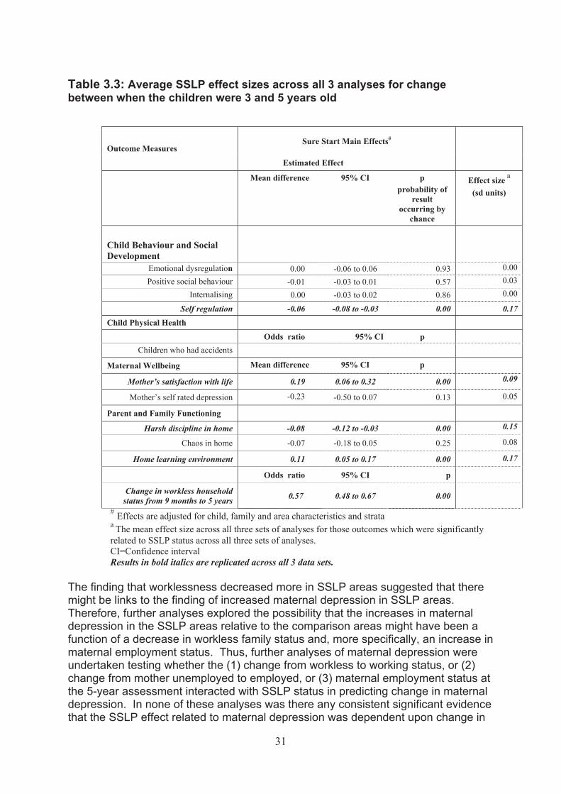
Table 3.3: Average SSLP effect sizes across all 3 analyses for change between when the children were 3 and 5 years old

Outcome Measures Sure Start Main Effects#

Estimated Effect

Mean difference 95% CI p probability of

result occurring by

chance

Effect size a

(sd units)

Child Behaviour and Social Development

Emotional dysregulation 0.00 -0.06 to 0.06 0.93 0.00

Positive social behaviour -0.01 -0.03 to 0.01 0.57 0.03

Internalising 0.00 -0.03 to 0.02 0.86 0.00

Self regulation -0.06 -0.08 to -0.03 0.00 0.17 Child Physical Health

Children who had accidents Odds ratio 95% CI p

Maternal Wellbeing

Mother’s satisfaction with life

Mother’s self rated depression

Mean difference 95% CI p

0.19 0.06 to 0.32 0.00

-0.23 -0.50 to 0.07 0.13

0.09

0.05

Parent and Family Functioning

Harsh discipline in home -0.08 -0.12 to -0.03 0.00 0.15

Chaos in home -0.07 -0.18 to 0.05 0.25 0.08

Home learning environment

Change in workless household status from 9 months to 5 years

0.11 0.05 to 0.17 0.00

Odds ratio 95% CI p

0.57 0.48 to 0.67 0.00

0.17

# Effects are adjusted for child, family and area characteristics and strata a The mean effect size across all three sets of analyses for those outcomes which were significantly related to SSLP status across all three sets of analyses. CI=Confidence interval Results in bold italics are replicated across all 3 data sets.

The finding that worklessness decreased more in SSLP areas suggested that there might be links to the finding of increased maternal depression in SSLP areas. Therefore, further analyses explored the possibility that the increases in maternal depression in the SSLP areas relative to the comparison areas might have been a function of a decrease in workless family status and, more specifically, an increase in maternal employment status. Thus, further analyses of maternal depression were undertaken testing whether the (1) change from workless to working status, or (2) change from mother unemployed to employed, or (3) maternal employment status at the 5-year assessment interacted with SSLP status in predicting change in maternal depression. In none of these analyses was there any consistent significant evidence that the SSLP effect related to maternal depression was dependent upon change in

31

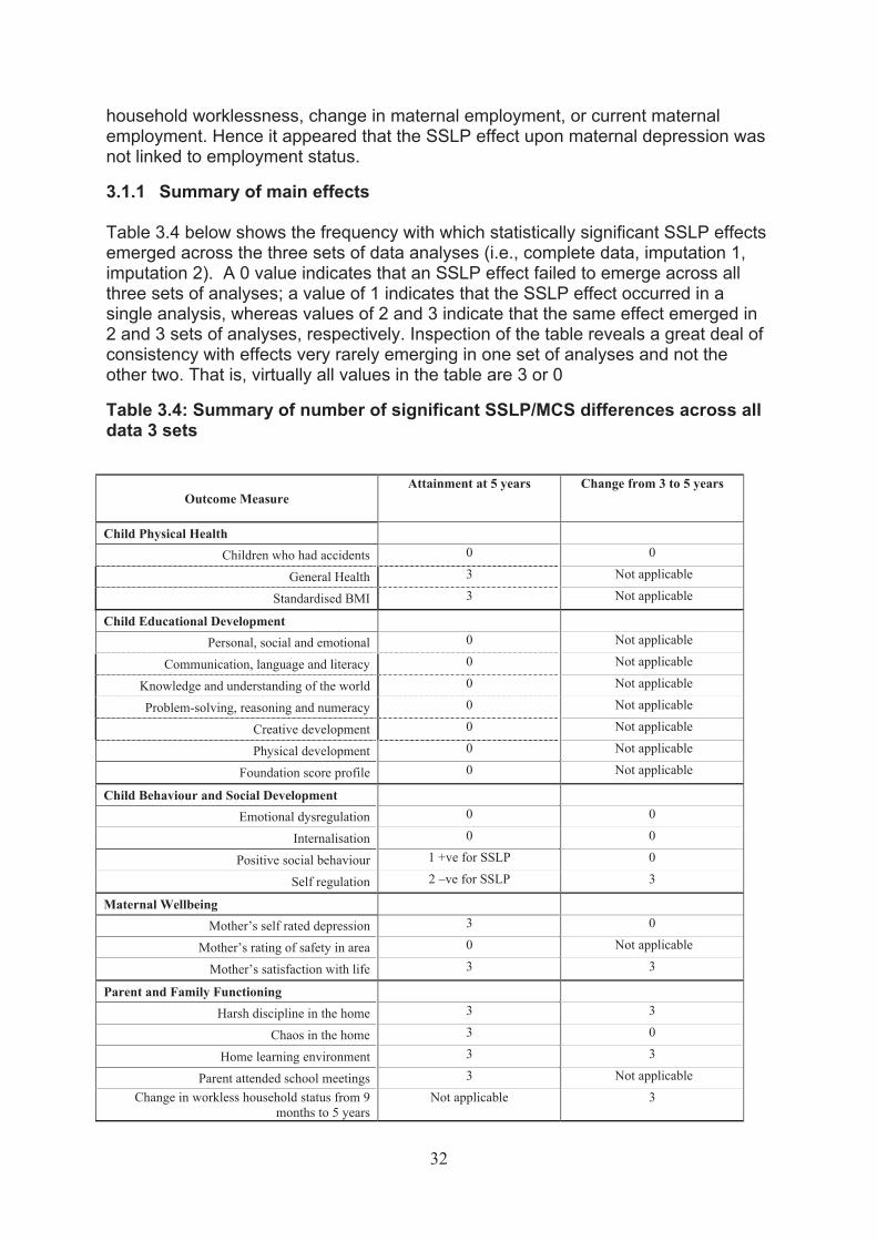
household worklessness, change in maternal employment, or current maternal employment. Hence it appeared that the SSLP effect upon maternal depression was not linked to employment status.

3.1.1 Summary of main effects

Table 3.4 below shows the frequency with which statistically significant SSLP effects emerged across the three sets of data analyses (i.e., complete data, imputation 1, imputation 2). A 0 value indicates that an SSLP effect failed to emerge across all three sets of analyses; a value of 1 indicates that the SSLP effect occurred in a single analysis, whereas values of 2 and 3 indicate that the same effect emerged in 2 and 3 sets of analyses, respectively. Inspection of the table reveals a great deal of consistency with effects very rarely emerging in one set of analyses and not the other two. That is, virtually all values in the table are 3 or 0

Table 3.4: Summary of number of significant SSLP/MCS differences across all data 3 sets

Outcome Measure Attainment at 5 years Change from 3 to 5 years

Child Physical Health Children who had accidents 0 0

General Health 3 Not applicable

Standardised BMI 3 Not applicable

Child Educational Development Personal, social and emotional 0 Not applicable

Communication, language and literacy 0 Not applicable

Knowledge and understanding of the world 0 Not applicable

Problem-solving, reasoning and numeracy 0 Not applicable

Creative development 0 Not applicable

Physical development 0 Not applicable

Foundation score profile 0 Not applicable

Child Behaviour and Social Development Emotional dysregulation 0 0

Internalisation 0 0

Positive social behaviour 1 +ve for SSLP 0

Self regulation 2 –ve for SSLP 3

Maternal Wellbeing Mother’s self rated depression 3 0

Mother’s rating of safety in area 0 Not applicable

Mother’s satisfaction with life 3 3

Parent and Family Functioning Harsh discipline in the home

Chaos in the home Home learning environment

Parent attended school meetings Change in workless household status from 9

months to 5 years

3 3 3 3

Not applicable

3 0 3

Not applicable 3

32

Across 21 dependent 5-year variables or outcomes evaluated, significant main or across-the-board effects of SSLPs emerged in the case of 8 outcomes. Indeed, after taking into consideration pre-existing family and area background characteristics (in all sets of analyses), the three sets of analyses comparing children and families living in SSLP areas and those living in similar areas not receiving SSLPs revealed 6 apparently positive and 2 apparently negative effects of SSLPs. On the positive front, mothers in SSLP areas reported greater life satisfaction, while engaging in less harsh discipline and providing a less chaotic and more cognitively stimulating home learning environment than their counterparts from the MCS who did not live in SSLP areas. Additionally, children growing up in SSLP areas had lower BMIs and better physical health than those residing in comparison communities. Mothers in SSLP areas, however, experienced more depressive symptoms and were less likely to attend school meetings than those in comparison areas. There are standard criteria for underweight, normal, overweight and obese classification published by the World Health Organisation (2008). Additional analyses thus determined whether the discerned SSLP effect on BMI was a function of SSLPs influencing the probability of a child being underweight, overweight or obese. These analyses revealed that while children in SSLP areas were less likely to be overweight—and thus were healthier in terms of BMI--than those in non-SSLP areas, their probability of being underweight or obese was similar to children growing up in non-SSLP areas.

With regard to change from age 3 to age 5 years, of 11 repeatedly measured dependent variables, 5 indicated SSLP effects on change over time in child or parent functioning in all three sets of analyses. Mothers in SSLP areas experienced more positive change in 4 outcome measures relative to those residing in MCS comparison areas in satisfaction with life (i.e. greater increase), while evincing more positive change as well in the home learning environment (i.e. greater improvement) and in harsh discipline (i.e. greater decrease). There was also a greater decrease in workless household status from 9 months to 5 years of age for families in SSLP areas. Children in SSLP areas, however, manifested less positive change in self regulation over time than those in non-SSLP areas, in that children in non-SSLP areas appeared to be catching-up with those in SSLP areas.

3.2 Second Stage: Did first stage analysis over/underestimate SSLP effects?

Recall that these across-the-board NESS-MCS comparisons just summarised did not involve substantial numbers of NESS children/families—those from Strata 1 and 5—due to the fact that there were insufficient numbers of these children/families in the MCS sample in stratum 5 or in the NESS sample in stratum 1 to afford reliable comparisons between MCS and NESS samples. To determine whether the (main) effects of SSLPs detected and reported in the preceding section might have been different had it proven possible to include all NESS children/families in the main comparisons presented in Table 3.2, a second stage of analysis was conducted comparing all NESS children and families from stratum 2-5 with one another on the outcome variables (after adjusting for all covariates); recall that strata 1 included very few NESS children/families and so was excluded from this analysis. If the within-NESS comparisons involving stratum 2-5 revealed differential functioning of

33

the NESS children/families not included in the NESS-MCS comparison, this would suggest that the NESS-MCS comparisons just reported might have either overestimated or underestimated SSLP effects.

The results of this second stage of analysis—across all 3 data sets (i.e. complete and imputed 1 and imputed 2)--revealed that NESS children/families from Strata 5 did not differ on any dependent measures from those in Strata 2-4 (see Table 3.4) after adjusting for background characteristics. This suggests that had it been possible to include Strata 5 children in the analysis reported in the preceding section doing so would not have changed the results reported earlier and thus those SSLP main effects discerned in the preceding analysis are generalisable to Strata-5 children/families. Clearly, this is an argument by inference and cannot be regarded as an indisputable conclusion.

3.3 Third Stage: Differential Effects of SSLPs on Specific Subpopulations

Having detected multiple indications of positive and negative effects of SSLPs on children and families when children were 5 years of age and in change from 3 to 5 years, as well as having found that these appear to apply to children and families of all SSLPs (i.e., even the most deprived areas excluded from the main analysis), the third stage of analysis was designed to determine whether effects of SSLPs were the same across various population sub-groups. This issue is particularly important given early findings from the initial cross-sectional study of 3-year olds showing that various demographically-defined sub-populations were differentially affected by SSLPs (NESS, 2005a; see also Belsky & Melhuish, 2007; Belsky et al., 2006).

In order to examine the prospect that SSLP effects varied across select subpopulations served by the programme, six demographic variables, were chosen, because of their policy relevance, to address the issue of sub-population-specific effects of SSLPs. More specifically, 2-way interactions involving SSLP status (NESS or MCS samples) and each of the following factors were tested for each outcome measure after controlling for the child, family and area characteristics (again using only Strata 2-4 children/families): x child gender x ethnicity x teenage parenthood (i.e. <20 years at delivery) x lone parenthood (i.e. no partner living in home) x workless household (i.e. no adult employed in home), and x household deprivation (i.e. <210 p.w., >£210 p.w. or below poverty line)

(Note: The £210 p.w. income figure was chosen as this was 60% of the median income for the country at the time of the 9-month data collection, and people with incomes below this figure are officially regarded as poor.)

As inspection of Table 3.5 indicates, there were only 3 significant interactions involving SSLP status (NESS/MCS) and demographic factors in the prediction of 5-

34

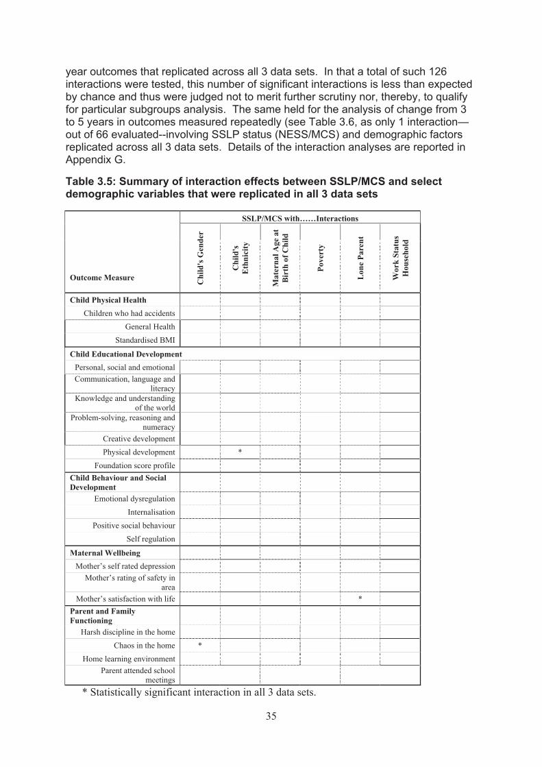
year outcomes that replicated across all 3 data sets. In that a total of such 126 interactions were tested, this number of significant interactions is less than expected by chance and thus were judged not to merit further scrutiny nor, thereby, to qualify for particular subgroups analysis. The same held for the analysis of change from 3 to 5 years in outcomes measured repeatedly (see Table 3.6, as only 1 interaction— out of 66 evaluated--involving SSLP status (NESS/MCS) and demographic factors replicated across all 3 data sets. Details of the interaction analyses are reported in Appendix G.

Table 3.5: Summary of interaction effects between SSLP/MCS and select demographic variables that were replicated in all 3 data sets

SSLP/MCS with……Interactions

Outcome Measure Chi

ld's

Gen

der

Chi

ld's

Eth

nici

ty

Mat

erna

l Age

at

Bir

th o

f Chi

ld

Pove

rty

Lon

e Pa

rent

Wor

k St

atus

Hou

seho

ld

Child Physical Health Children who had accidents

General Health Standardised BMI

Child Educational Development Personal, social and emotional Communication, language and

literacy Knowledge and understanding

of the world Problem-solving, reasoning and

numeracy Creative development Physical development *

Foundation score profile Child Behaviour and Social Development

Emotional dysregulation Internalisation

Positive social behaviour Self regulation

Maternal Wellbeing Mother’s self rated depression

Mother’s rating of safety in area

Mother’s satisfaction with life * Parent and Family Functioning

Harsh discipline in the home Chaos in the home *

Home learning environment Parent attended school

meetings * Statistically significant interaction in all 3 data sets.

35

Outcome Measure

SSLP/MCS with……Interactions

Chi

ld's

Gen

der

Chi

ld's

Eth

nici

ty

Mat

erna

l Age

at

Bir

th o

f Chi

ld

Pove

rty

Lon

e Pa

rent

Wor

k St

atus

Hou

seho

ld

Child Behaviour and Social Development

Emotional dysregulation Internalisation

Positive social behaviour Self regulation

Child Physical Health

Children who had accidents

Maternal Wellbeing Mother’s self rated depression Mother’s satisfaction with life *

Parent and Family Functioning

Harsh discipline in the home Chaos in the home

Home learning environment Change in working/workless household status from when

child is 9months to 5 years old

Table 3.6: Summary of interaction effects between SSLP/MCS and select demographic variables for models of change 3 to 5 years that were replicated for all 3 data sets

* Statistically significant in all 3 data sets

36

3.4 Fourth Stage: Threats to confidence in detected SSLP effects

Given the circumstances under which the NESS Impact Study was carried out, the MCS element of which was not under the control of the NESS Impact Study team, there are certain threats to the confidence that can be placed in the SSLP effects reported. Significantly, because there was selective attrition within each of the samples studied, NESS and MCS, the possibility exists that the results are biased as a result of this.

Recall that in both samples some children seen at 3 years were not seen again at age 5. In light of this, it is reasonable to ask whether the SSLP effects detected would generalise to children/families not seen at age 5. To address this issue, the NESS children and families seen at 3 years but not at 5 years were compared on a range of demographic variables with those seen on both occasions, separately by strata (i.e. attrition group vs. strata1; attrition group vs. strata 2…) (see Appendix B). If the NESS children/families not seen at age 5 proved more deprived than those seen at both ages of measurement—and, especially, more deprived than those in stratum 5--this would undermine confidence in the interpretation attributed to the discovery reported in the second stage of analyses that stratum 5 children/families were not different from those in strata 2-4. After all, it was this absence of difference that provided the basis for the earlier observation that the SSLP effects detected in the first stage of inquiry—which only involved strata 2-4—probably generalised to stratum 5 children/families, that is, those most likely to be in SSLP areas.

The attrition analysis revealed that risks arising from selective attrition appear not to seriously threaten the confidence to be placed in the SSLP effects detected in the first stage of analysis (and, which were found, in the second stage of analysis, to be probably generalisable to stratum 5 children). This is because on some measures one sample appeared more disadvantaged, whereas on other measures the reverse was the case. Specifically, although the NESS sub-sample not seen at age 5 proved to be significantly less advantaged than those in strata 1, 2, 3 and 4 seen at both 3 and 5 years, of the eight variables that indicate a significant difference between the sample seen at 5 years of age and those not seen at five years of age, four variables (i.e. teen mother, lone parent, workless household, parent education) indicate that the sample seen at 5 years in stratum 5 are less disadvantaged, and four variables (i.e. ethnicity, English First language, below poverty line, parent occupation) indicate that the sample seen at 5 years in stratum 5 are more disadvantaged than the attrition group (not seen at 5 years of age). This suggests that had the attrition group also been followed up at age 5 the absence of differences on test outcomes between stratum 5 and the other strata would have remained. Once again this would lead to the conclusion that the results from the first stage of analysis involving only strata 2-4 sub-samples appear generalisable to stratum-5 children/families, those most likely to be in SSLP areas.

37

4. SUMMARY

In the evaluation of child and family functioning at 5 years, evidence of 6 beneficial and 2 adverse SSLP effects emerged in this quasi-experimental investigation. Across 21 dependent variables or outcomes evaluated4, significant main or across-the-board effects of SSLPs on age-5 functioning emerged in the case of these 8 outcomes after taking into consideration pre-existing family and area background characteristics (in all sets of analyses). There was limited evidence that SSLPs benefited children directly, including in terms of ’school readiness’ (FSP scores). Nevertheless, on the positive front, mothers in SSLP areas reported greater life satisfaction, while engaging in less harsh discipline and providing a less chaotic and more cognitively stimulating home learning environment than their counterparts from the MCS who did not live in SSLP areas. Additionally, children growing up in SSLP areas had lower BMIs, due to the fact that they were less likely to be overweight, and better physical health than those residing in comparison communities. Mothers in SSLP areas, however, experienced more depressive symptoms and were less likely to attend school meetings than those in comparison areas. Finally, no differences emerged between the NESS and MCS groups on 7 measures of cognitive and social development from the Foundation Stage Profile completed by teachers, 4 measures of socio-emotional development based on mothers’ ratings, and mothers’ ratings of area safety.

Examination of change over time in child and family function as a function of living in an SSLP area, yielded SSLP effects on 5 of 11 repeatedly measured dependent variables in all three sets of analyses; once again, though, there was little direct evidence of children benefiting from residing in SSLP areas. Nevertheless, mothers in SSLP areas experienced more positive change relative to those residing in MCS comparison areas in terms of satisfaction with life (i.e. greater increase), while evincing more positive change as well in the home learning environment (i.e. greater improvement) and in harsh discipline (i.e. greater decrease). There was also a greater decrease in workless household status from 9 months to 5 years of age for families in SSLP areas. Children in SSLP areas, however, manifested less positive change in self regulation over time than those in non-SSLP areas, in that children in non-SSLP areas appeared to be catching-up with those in SSLP areas. The adverse effects of SSLPs on maternal depression at the 5-year measurement could not be attributed neither to change in workless household status or maternal employment status from 9 months to 5 years nor to maternal employment status at 5 years. Finally, there were no differences associated with SSLPs for change in child emotional dysregulation, positive social behaviour or internalising behaviour as rated by parents, child accidents, mother’s depression, or chaotic home environments.

The SSLP effects just summarised appeared generalisable across population sub-groups (e.g. workless households, teen mothers) for two reasons: (1) In general, differences in SSLP effects across subgroups emerged less frequently than would be expected by chance; and, (2) there was almost no consistent evidence that children and families in the most disadvantaged SSLP areas, which had more of the most disadvantaged families, functioned differently to children and families in somewhat less disadvantaged SSLP areas.

4 Definitions of outcomes can be found in Appendix C.

38

5. CONCLUSION

In order to interpret these findings some important points that constrain conclusions need to be reiterated.

Methodological Constraints Under ideal scientific circumstances areas would have been randomly assigned to receive an SSLP or not. This would permit the strongest policy-related conclusions. It also would have been beneficial to have data on children/families in SSLP and non-SSLP areas collected by the same research team and at the same time. The fact that this was not the case weakened the NESS Impact Study in ways beyond the control of the NESS team. In particular the two year gap between the measurements in the NESS and MCS samples meant that with the exception of the child educational (FSP) data, any and all discerned effects of SSLPs—whether positive or negative in character--potentially could be attributed to time-related changes in communities and/or the larger society that had nothing to do with SSLPs.

These constraints highlight the importance of giving early consideration, during the planning phase of an evaluation, to the trade-offs involved in compromising on fundamental evaluation design issues.

Having covered the limitations of the NESS Impact Study evaluation, we now proceed to review what emerged from this third phase of investigation.

Detected “effects” of SSLPs on Children/Families To take account of missing data effectively the decision was made to evaluate SSLP effects in three different ways. Whereas one set of analyses only included those seen at age 5 with complete measurement data, two other sets of analyses were based on multiple imputation of missing data. One involved imputing missing data on any cases seen at age 5, whereas the other involved imputing missing data on any cases seen at age 3. Evaluation of SSLP effects involved both child/family functioning at age 5 and change from age 3-5 in child/family functioning for 10 repeatedly measured outcomes and change from 9 months to 5 years in household workless status (i.e. 11 change analyses). Finally, detected effects of SSLPs were only judged to be meaningful and thus worthy of consideration if they proved significant across all three sets of analyses—which most detected effects did.

After taking into consideration pre-existing family and area background characteristics six positive and two negative effects of SSLPs emerged from 21 measured outcomes at age 5. On the positive front, mothers in SSLP areas reported (1) greater life satisfaction, while (2) engaging in less harsh discipline and (3) providing a less chaotic and (4) more cognitively stimulating home learning environment than their counterparts who did not live in SSLP areas. Additionally, children growing up in SSLP areas had (5) lower BMIs, due to the fact that they were less likely to be overweight and thus healthier in terms of BMI, even if not less likely to be obese per se; and (6) better physical health than those residing in comparison communities. Mothers in SSLP areas, however, (7) experienced more depressive symptoms and (8) were less likely to attend school meetings than those in comparison areas.

39

Additional evidence of both positive and negative SSLP effects emerged on 5 of 11 repeatedly-measured outcomes when the focus of evaluation was on change in parent and child functioning from age 3 to 5. Once again the evidence was mixed with four beneficial and one adverse effect of SSLPs being identified. Mothers in SSLP areas relative to those residing in comparison areas (1) experienced a greater increase in satisfaction with life, while (2) evincing a greater improvement in the home learning environment and (3) a greater decrease in harsh discipline. There was also a (4) greater decrease in workless household status from 9 months to 5 years of age for families in SSLP areas. Children in SSLP areas, however, (5) manifested less positive change in self regulation over time than those in non-SSLP areas in that children in non-SSLP areas appeared to be catching-up with those in SSLP areas.

All of the SSLP effects just described appeared generalisable across population sub-groups (e.g. workless households, teen mothers) for two reasons: (1) In general, differences in SSLP effects across subgroups—as evaluated by statistical interactions between SSLP status and select demographic factors—emerged less frequently than would be expected by chance; and, (2) there was almost no consistent evidence that children and families in the most disadvantaged SSLP areas (i.e. strata 5), with more of the most disadvantaged families, differed in functioning to children and families in somewhat less disadvantaged SSLP areas (i.e. strata 2-4).

In some respects the results from this third phase of the NESS Impact Study are somewhat reminiscent of those discerned in the earliest phase of assessment. Like the first phase (NESS, 2005; Belsky et al., 2005), this phase of investigation revealed mixed SSLP effects, most being positive/beneficial in nature and a couple being negative in character. This time, however, it was not the case as in the first phase that different subgroups were found to benefit and to be adversely affected; instead, the positive and negative effects discerned applied equally to all subgroups.

It is encouraging that beneficial effects of SSLPs proved more frequent than negative effects in this 5-year-assessment phase, making this third stage of inquiry more like the second phase in which only positive effects emerged when children were 3 years of age (NESS, 2008; Melhuish et al., 2008a). Exactly why some negative effects have also emerged is unclear and post-hoc explanations may be inappropriate given that all SSLP effects reported are small and could be an artefact of time of measurement, due to the two-year gap between MCS and NESS measurements. The significance of these effects is likely to be clearer once age-7 data are analysed.

On the positive side, the results discerned in this third phase of the NESS Impact Study provide some support for the view that government efforts to support children/families via the original area-based approach to Sure Start paid off, at least to some degree, even if some negative effects resulted as well. Nevertheless, the fact that effect sizes proved modest and, child functioning, with the exception of child BMI and physical health, did not show benefits, raises questions about “return on investment”. This is particularly the case with regard to “school readiness” or children’s capabilities to succeed in school as a result of academic and social skills,

40

at least as measured by FSP scores.

It might be thought that SSLP effects upon parenting would feed through to detectable improvements in child outcomes. Although this was evident at 3 years, no such evidence emerged at 5 years. While the effect sizes for parenting are the strongest effects detected, they are relatively small, and any consequent effect upon child development may simply be too small to detect.

The main evidence for population-wide early years programmes affecting child development concerns high quality pre-school education being associated with improved cognitive and social development (Belsky et al., 2007; Melhuish et al., 2008b; Sylva et al., 2010). While pre-school education is part of what SSLPs (now children’s centres) offer, it will also be available to children in non-SSLP areas. From 2004, the Government introduced regulations that gave an entitlement to 12.5 hours of free childcare a week to all 3 and 4 year olds and 95% of the eligible children in England take up this offer (DfE, June 2010). Hence there are unlikely to be differences in pre-school education experiences, for which evidence related to child development is strongest, between children in or not in SSLP areas. This equivalence of pre-school education experience could be responsible for the failure to detect SSLP effects on children at age 5 (apart from physical health measures) in this evaluation. That is, it could be the case that developmental advantages associated with SSLPs at age 3 prove non-existent at age 5 because by this time all children are being exposed to pre-school provision, which results in “catch up” for those children in non-SSLP areas. The report on pre-school childcare in SSLP areas published alongside this report considers the quality of pre-school provision in SSLP areas and any links with child outcomes. It may also be the case that, as opposed to standardised individual assessments of children, the FSP teacher completed information is not sufficiently fine-grained to identify group differences.

The fact that adverse effects emerged, even if those effects were very small and occurred less frequently than positive effects, necessitates caution in embracing any claim that SSLPs proved effective in enhancing child and family functioning, whether on a cost-effective basis or not. In fact, the negative effects discerned are difficult to reconcile with the positive effects detected. Why, for example, should a programme that seems to have a positive effect on a mother’s sense of life satisfaction also seem to generate a negative effect on depression, especially as these are not unrelated psychological constructs? By the same token, why should it be that depressive symptoms are promoted by SSLP exposure at the same time that parenting and the family environment is enhanced? This is especially perplexing given extensive theory and evidence that depression undermines parenting and family functioning.

It might be attractive to propose that SSLP mothers report more depressive symptoms because they are more attuned to their own feelings which, in the long run, will enhance their own, their families’ and their children’s well being. On the other hand one could just as easily contend that mothers in SSLP areas have learnt to report positive parenting behaviours. It would seem wiser to see whether the SSLP effects detected in this inquiry, whether beneficial or adverse, are replicated at age 7 before rushing to judgment. The educational outcomes to be examined at age 7 derive from National Assessment data that will be standardised by year of

41

collection, thus avoiding the problem of possible ‘time of measurement’ effect (as was done with FSP data). Results that replicate across time periods can be treated with much more confidence.

Sure Start has undergone evolutionary change since its inception in 1998. To some extent evaluation results have influenced this process. The early results indicated that lack of specification of how goals are to be achieved in service delivery will lead to great programme diversity. Later developments have tightened up guidelines and the nature of service delivery considerably and also staff themselves have developed and become better trained and more proficient. However, there is still scope for further development. The contrast between the first cross-sectional and subsequent Impact Study findings suggests that children and families who have had greater exposure to SSLPs/children’s centres that have had more time to ‘bed-in’ and develop, indicates that such early interventions may be increasingly effective in improving the life chances of young children in deprived areas. Nonetheless, it is clear that further developments are desirable. In particular, language development in the early years underpins both cognitive and social development. Hence if children’s centres are to have an observable impact upon school readiness greater emphasis needs to be given to improving children’s language development. In the meantime, it will be some time before the longer term goals of the programme can be realised, and hence the final verdict on Sure Start Local Programmes awaits further evaluation.

Final Comments

SSLPs appear to have generated mainly positive, but also some negative effects by the time children are 5 years of age. Primarily the benefits apply to parenting behaviour and only in the case of physical health did children directly benefit. It is disappointing that no effects were discerned for “school readiness” as measured by the Foundation Stage Profile, and further work is exploring how pre-school childcare provided by children’s centres might improve child development outcomes including “school readiness”.

�

42

REFERENCES

Barnes, J., (2007) Targeting Deprived Areas: The Nature of the Sure Start Local Programme Neighbourhoods In J. Belsky, J. Barnes, & E. Melhuish, (Eds.). The National Evaluation of Sure Start: Does Area-based Early Intervention Work? Bristol, UK: The Policy Press.

Belsky, J., Barnes, J., & Melhuish, E. (Eds.). (2007). The National Evaluation of Sure Start: Does Area-based Early Intervention Work? Bristol, UK: The Policy Press.

Belsky, J., & Melhuish, E. (2007). Impact of Sure Start local Programmes on Children and Families. In J. Belsky, J. Barnes, & E. Melhuish, (Eds.). The National Evaluation of Sure Start: Does Area-based Early Intervention Work? Bristol, UK: The Policy Press.

Belsky, J., Melhuish, E., Barnes, J., Leyland, A.H., Romaniuk, H., & the NESS Research Team. (2006). Effects of Sure Start Local Programmes on Children and Families: Early Findings from a Quasi-experimental, Cross-sectional Study. BMJ, 332, 1476-1578 (published at BMJonline: ttp://bmj.com/cgi/doi/10.1136/bmj.38853.451748.2F).

Belsky, J., Vandell, D. Burchinal, M. Clarke-Stewart, K.A., McCartney, K., Owen, M. & The NICHD Early Child Care Research Network (2007). Are There Long-term Effects of Early Child Care? Child Development, 78, 681-701.

DfE (2010). Statistical First Release: Provision for Children Under Five Years of Age in England - June 2010. Available at: http://www.dcsf.gov.uk/rsgateway/DB/SFR/s000935/index.shtml

DCSF (2009). Statistical First Release: Early Years Foundation Stage Profile Results in England 2008/09. SFR 26/2009. Available at: http://www.dcsf.gov.uk/rsgateway/DB/SFR/s000879/SFR26_2009.pdf

Elliot, C, with Smith, P., and McCulloch, K. (1996). British Ability scales: 2nd edition. Windsor: NFER-Nelson.

Frost, M., & Harper, G. (2007). The challenge of profiling communities. In J. Belsky, J. Barnes, & E. Melhuish, E. (Eds.). The National Evaluation of Sure Start: Does Area-based Early Intervention Work? Bristol, UK: The Policy Press.

Hill, J.L., Waldfogel, J., Brooks-Gunn, J. & Han, W. (2005). Maternal employment and child development: A fresh look using new methods. Developmental Psychology, 41, 833-850.

HM Treasury (1998a). Modern Public Services for Britain: Investing in Reform. Comprehensive Spending Review: New Public Spending Plans. London: HMSO.

HM Treasury (1998b). Comprehensive Spending Review: Cross Departmental Review of Provision for Young Children. London: HMSO.

Love, J., Kisker, E. E., Ross, C. M. Schochet, P. Z., Brooks-Gunn, J., Paulsell, D., Boller, K., Constantine, J., Vogel, C., Fuligni, A. S., Brady-Smith, C. (2002). Making a

43

difference in the lives of infants and toddlers and their families: The impacts of Early Head Start. Volume 1: Final Technical Report. Princeton, NJ: Mathematica Policy Research Inc. Available at: http://www.mathematica-mpr.com/PDFs/ehsfinalvol1.pdf

McCartney, K., Bub, K., & Burchinal, M. (2006). Selection, detection and reflection. In K. McCartney, Burchinal, M.R., & Bub, K. (Eds.), Best practices in quantitative methods (pp. 105-126). Monographs of the Society for Research in Child Development, Serial 285, Vol. 71.

Melhuish E. & Hall D. (2007). The policy background to Sure Start. In: Belsky J, Barnes J, Melhuish E, Eds. The National Evaluation of Sure Start: Does Area-based early intervention work? Bristol: Policy Press, pp 3-21.

Melhuish, E. Belsky, J., Leyland, A.H., Barnes, J. & NESS Research Team (2008a). Effects of fully-established Sure Start Local Programmes on 3-year-old children and their families living in England: a quasi-experimental observational study. Lancet, 372, 1641-1647.

Melhuish, E.C., Sylva, K., Sammons, P., Siraj-Blatchford, I., Taggart, B., Phan, M. & Malin, A. (2008b). Preschool influences on mathematics achievement. Science, 321, 1161-1162.

NESS Research Team (2005). Early impacts of Sure Start Local Programmes on Children and Families. Report 13. London: Department for Education and Skills, www.surestart.gov.uk/doc/P0001867.pdf

NESS Research team (2008). The impact of Sure Start Local Programmes on three year olds and their families. London: DCSF.

ODPM. (2004), The English Indices of Deprivation 2004 (revised). London: ODPM.

Olds, D. L., Henderson, C.R., Kitzman, H., Eckenrode, J. J., Cole, R. E., & Tatelbaum, R. C. (1999). “Prenatal and Infancy Home visitation by Nurses: recent Findings,” Future of Children, 9, 44-66.

Pearl, J. (2009). Causality: Models, Reasoning, and Inference, 2nd Ed. Cambridge: CUP.

Ramey, C. T., Campbell, F. A., Burchinal, M., Skinner, M. L., Gardner, D. M., & Ramey, S. L. (2000). Persistent Effects of Early Childhood Education on High-risk Children and their Mothers. Applied Developmental Science, 4(1), 2-14

Rosenbaum, P. R., Rubin, D. B. (1983). "The central role of the propensity score in observational studies for causal effects". Biometrika, 70 (1): 41–55.

Rubin, D.B. (1987) Multiple Imputation for Non-response in Surveys. London: Wiley.

Rubin, D.B. (1997). Estimating causal effects from large datasets using propensity scores. Annals of Internal Medicine, 127, 757-763.

44

Sammons, P., Sylva, K., Melhuish, E., Siraj-Blatchford, I., Taggart, B., and Hunt, S. (2008). Influences on Children’s Attainment and Progress in Key Stage 2: Cognitive outcomes in Year 6. London: DCSF

Sylva, K., Melhuish, E., Sammons, P., Siraj-Blatchford, I. and Taggart, B., (Eds) (2010). Early Childhood Matters: Evidence from the Effective Pre-school and Primary Education Project. London: Routledge.

WHO 2008. Growth Reference charts http://www.who.int/growthref/who2007_bmi_for_age/en/index.html

45

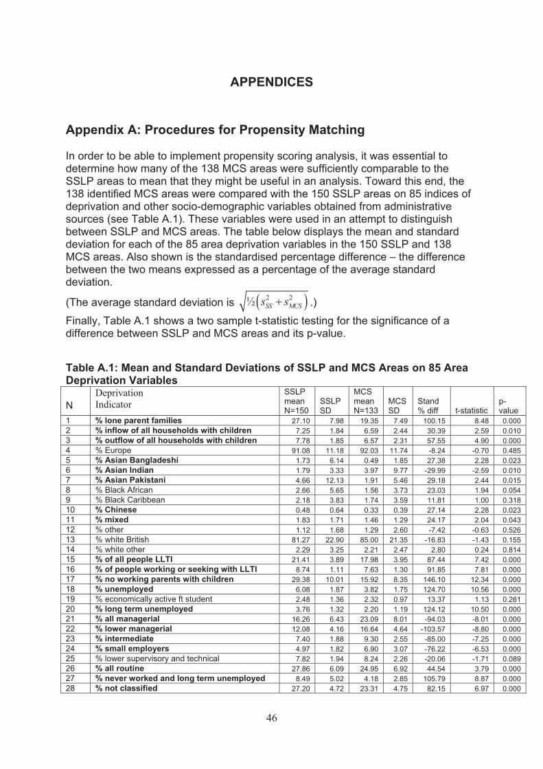
APPENDICES

Appendix A: Procedures for Propensity Matching

In order to be able to implement propensity scoring analysis, it was essential to determine how many of the 138 MCS areas were sufficiently comparable to the SSLP areas to mean that they might be useful in an analysis. Toward this end, the 138 identified MCS areas were compared with the 150 SSLP areas on 85 indices of deprivation and other socio-demographic variables obtained from administrative sources (see Table A.1). These variables were used in an attempt to distinguish between SSLP and MCS areas. The table below displays the mean and standard deviation for each of the 85 area deprivation variables in the 150 SSLP and 138 MCS areas. Also shown is the standardised percentage difference – the difference between the two means expressed as a percentage of the average standard deviation.

2 2(The average standard deviation is ½� s � s � .)SS MCS

Finally, Table A.1 shows a two sample t-statistic testing for the significance of a difference between SSLP and MCS areas and its p-value.

Table A.1: Mean and Standard Deviations of SSLP and MCS Areas on 85 Area Deprivation Variables

N Deprivation Indicator

SSLP mean N=150

SSLP SD

MCS mean N=133

MCS SD

Stand % diff t-statistic

p-value

1 % lone parent families 27.10 7.98 19.35 7.49 100.15 8.48 0.000 2 % inflow of all households with children 7.25 1.84 6.59 2.44 30.39 2.59 0.010 3 % outflow of all households with children 7.78 1.85 6.57 2.31 57.55 4.90 0.000 4 % Europe 91.08 11.18 92.03 11.74 -8.24 -0.70 0.485 5 % Asian Bangladeshi 1.73 6.14 0.49 1.85 27.38 2.28 0.023 6 % Asian Indian 1.79 3.33 3.97 9.77 -29.99 -2.59 0.010 7 % Asian Pakistani 4.66 12.13 1.91 5.46 29.18 2.44 0.015 8 % Black African 2.66 5.65 1.56 3.73 23.03 1.94 0.054 9 % Black Caribbean 2.18 3.83 1.74 3.59 11.81 1.00 0.318 10 % Chinese 0.48 0.64 0.33 0.39 27.14 2.28 0.023 11 % mixed 1.83 1.71 1.46 1.29 24.17 2.04 0.043 12 % other 1.12 1.68 1.29 2.60 -7.42 -0.63 0.526 13 % white British 81.27 22.90 85.00 21.35 -16.83 -1.43 0.155 14 % white other 2.29 3.25 2.21 2.47 2.80 0.24 0.814 15 % of all people LLTI 21.41 3.89 17.98 3.95 87.44 7.42 0.000 16 % of people working or seeking with LLTI 8.74 1.11 7.63 1.30 91.85 7.81 0.000 17 % no working parents with children 29.38 10.01 15.92 8.35 146.10 12.34 0.000 18 % unemployed 6.08 1.87 3.82 1.75 124.70 10.56 0.000 19 % economically active ft student 2.48 1.36 2.32 0.97 13.37 1.13 0.261 20 % long term unemployed 3.76 1.32 2.20 1.19 124.12 10.50 0.000 21 % all managerial 16.26 6.43 23.09 8.01 -94.03 -8.01 0.000 22 % lower managerial 12.08 4.16 16.64 4.64 -103.57 -8.80 0.000 23 % intermediate 7.40 1.88 9.30 2.55 -85.00 -7.25 0.000 24 % small employers 4.97 1.82 6.90 3.07 -76.22 -6.53 0.000 25 % lower supervisory and technical 7.82 1.94 8.24 2.26 -20.06 -1.71 0.089 26 % all routine 27.86 6.09 24.95 6.92 44.54 3.79 0.000 27 % never worked and long term unemployed 8.49 5.02 4.18 2.85 105.79 8.87 0.000 28 % not classified 27.20 4.72 23.31 4.75 82.15 6.97 0.000

46

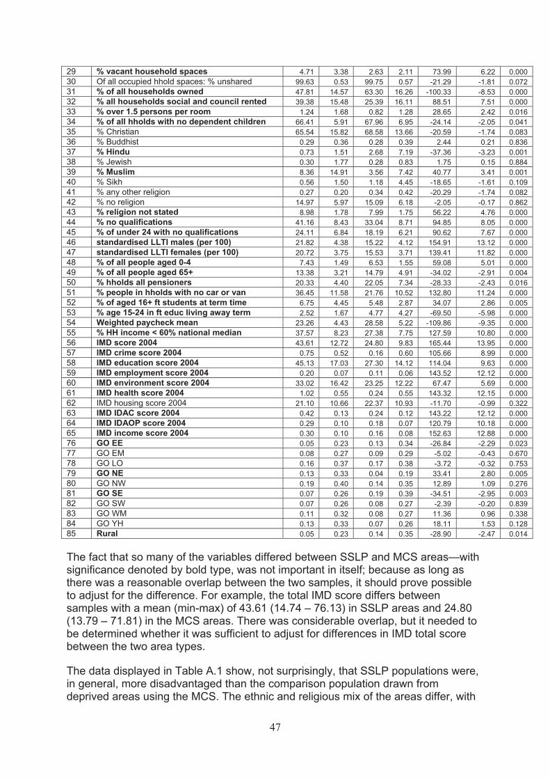
29 % vacant household spaces 4.71 3.38 2.63 2.11 73.99 6.22 0.000 30 Of all occupied hhold spaces: % unshared 99.63 0.53 99.75 0.57 -21.29 -1.81 0.072 31 % of all households owned 47.81 14.57 63.30 16.26 -100.33 -8.53 0.000 32 % all households social and council rented 39.38 15.48 25.39 16.11 88.51 7.51 0.000 33 % over 1.5 persons per room 1.24 1.68 0.82 1.28 28.65 2.42 0.016 34 % of all hholds with no dependent children 66.41 5.91 67.96 6.95 -24.14 -2.05 0.041 35 % Christian 65.54 15.82 68.58 13.66 -20.59 -1.74 0.083 36 % Buddhist 0.29 0.36 0.28 0.39 2.44 0.21 0.836 37 % Hindu 0.73 1.51 2.68 7.19 -37.36 -3.23 0.001 38 % Jewish 0.30 1.77 0.28 0.83 1.75 0.15 0.884 39 % Muslim 8.36 14.91 3.56 7.42 40.77 3.41 0.001 40 % Sikh 0.56 1.50 1.18 4.45 -18.65 -1.61 0.109 41 % any other religion 0.27 0.20 0.34 0.42 -20.29 -1.74 0.082 42 % no religion 14.97 5.97 15.09 6.18 -2.05 -0.17 0.862 43 % religion not stated 8.98 1.78 7.99 1.75 56.22 4.76 0.000 44 % no qualifications 41.16 8.43 33.04 8.71 94.85 8.05 0.000 45 % of under 24 with no qualifications 24.11 6.84 18.19 6.21 90.62 7.67 0.000 46 standardised LLTI males (per 100) 21.82 4.38 15.22 4.12 154.91 13.12 0.000 47 standardised LLTI females (per 100) 20.72 3.75 15.53 3.71 139.41 11.82 0.000 48 % of all people aged 0-4 7.43 1.49 6.53 1.55 59.08 5.01 0.000 49 % of all people aged 65+ 13.38 3.21 14.79 4.91 -34.02 -2.91 0.004 50 % hholds all pensioners 20.33 4.40 22.05 7.34 -28.33 -2.43 0.016 51 % people in hholds with no car or van 36.45 11.58 21.76 10.52 132.80 11.24 0.000 52 % of aged 16+ ft students at term time 6.75 4.45 5.48 2.87 34.07 2.86 0.005 53 % age 15-24 in ft educ living away term 2.52 1.67 4.77 4.27 -69.50 -5.98 0.000 54 Weighted paycheck mean 23.26 4.43 28.58 5.22 -109.86 -9.35 0.000 55 % HH income < 60% national median 37.57 8.23 27.38 7.75 127.59 10.80 0.000 56 IMD score 2004 43.61 12.72 24.80 9.83 165.44 13.95 0.000 57 IMD crime score 2004 0.75 0.52 0.16 0.60 105.66 8.99 0.000 58 IMD education score 2004 45.13 17.03 27.30 14.12 114.04 9.63 0.000 59 IMD employment score 2004 0.20 0.07 0.11 0.06 143.52 12.12 0.000 60 IMD environment score 2004 33.02 16.42 23.25 12.22 67.47 5.69 0.000 61 IMD health score 2004 1.02 0.55 0.24 0.55 143.32 12.15 0.000 62 IMD housing score 2004 21.10 10.66 22.37 10.93 -11.70 -0.99 0.322 63 IMD IDAC score 2004 0.42 0.13 0.24 0.12 143.22 12.12 0.000 64 IMD IDAOP score 2004 0.29 0.10 0.18 0.07 120.79 10.18 0.000 65 IMD income score 2004 0.30 0.10 0.16 0.08 152.63 12.88 0.000 76 GO EE 0.05 0.23 0.13 0.34 -26.84 -2.29 0.023 77 GO EM 0.08 0.27 0.09 0.29 -5.02 -0.43 0.670 78 GO LO 0.16 0.37 0.17 0.38 -3.72 -0.32 0.753 79 GO NE 0.13 0.33 0.04 0.19 33.41 2.80 0.005 80 GO NW 0.19 0.40 0.14 0.35 12.89 1.09 0.276 81 GO SE 0.07 0.26 0.19 0.39 -34.51 -2.95 0.003 82 GO SW 0.07 0.26 0.08 0.27 -2.39 -0.20 0.839 83 GO WM 0.11 0.32 0.08 0.27 11.36 0.96 0.338 84 GO YH 0.13 0.33 0.07 0.26 18.11 1.53 0.128 85 Rural 0.05 0.23 0.14 0.35 -28.90 -2.47 0.014

The fact that so many of the variables differed between SSLP and MCS areas—with significance denoted by bold type, was not important in itself; because as long as there was a reasonable overlap between the two samples, it should prove possible to adjust for the difference. For example, the total IMD score differs between samples with a mean (min-max) of 43.61 (14.74 – 76.13) in SSLP areas and 24.80 (13.79 – 71.81) in the MCS areas. There was considerable overlap, but it needed to be determined whether it was sufficient to adjust for differences in IMD total score between the two area types.

The data displayed in Table A.1 show, not surprisingly, that SSLP populations were, in general, more disadvantaged than the comparison population drawn from deprived areas using the MCS. The ethnic and religious mix of the areas differ, with

47

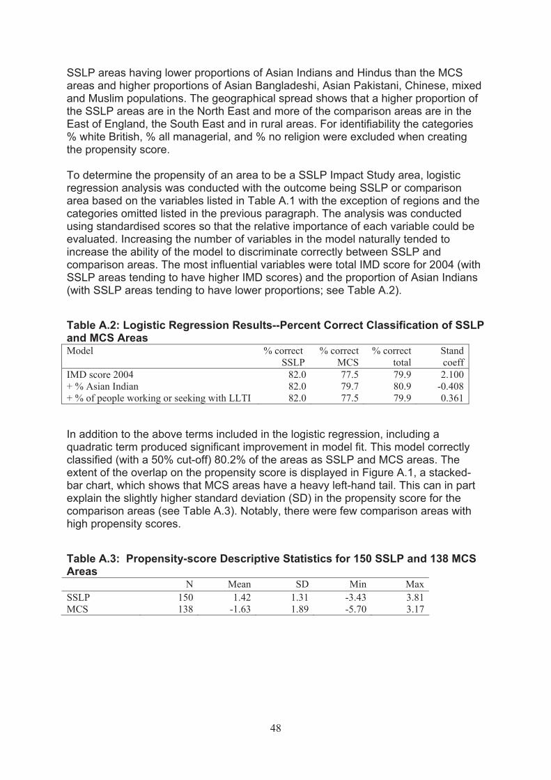
SSLP areas having lower proportions of Asian Indians and Hindus than the MCS areas and higher proportions of Asian Bangladeshi, Asian Pakistani, Chinese, mixed and Muslim populations. The geographical spread shows that a higher proportion of the SSLP areas are in the North East and more of the comparison areas are in the East of England, the South East and in rural areas. For identifiability the categories % white British, % all managerial, and % no religion were excluded when creating the propensity score.

To determine the propensity of an area to be a SSLP Impact Study area, logistic regression analysis was conducted with the outcome being SSLP or comparison area based on the variables listed in Table A.1 with the exception of regions and the categories omitted listed in the previous paragraph. The analysis was conducted using standardised scores so that the relative importance of each variable could be evaluated. Increasing the number of variables in the model naturally tended to increase the ability of the model to discriminate correctly between SSLP and comparison areas. The most influential variables were total IMD score for 2004 (with SSLP areas tending to have higher IMD scores) and the proportion of Asian Indians (with SSLP areas tending to have lower proportions; see Table A.2).

Table A.2: Logistic Regression Results--Percent Correct Classification of SSLP and MCS Areas Model % correct

SSLP % correct

MCS % correct

total Stand coeff

IMD score 2004 + % Asian Indian + % of people working or seeking with LLTI

82.0 82.0 82.0

77.5 79.7 77.5

79.9 80.9 79.9

2.100 -0.408 0.361

In addition to the above terms included in the logistic regression, including a quadratic term produced significant improvement in model fit. This model correctly classified (with a 50% cut-off) 80.2% of the areas as SSLP and MCS areas. The extent of the overlap on the propensity score is displayed in Figure A.1, a stacked-bar chart, which shows that MCS areas have a heavy left-hand tail. This can in part explain the slightly higher standard deviation (SD) in the propensity score for the comparison areas (see Table A.3). Notably, there were few comparison areas with high propensity scores.

Table A.3: Propensity-score Descriptive Statistics for 150 SSLP and 138 MCSAreas

N Mean SD Min Max SSLP 150 1.42 1.31 -3.43 3.81 MCS 138 -1.63 1.89 -5.70 3.17

48

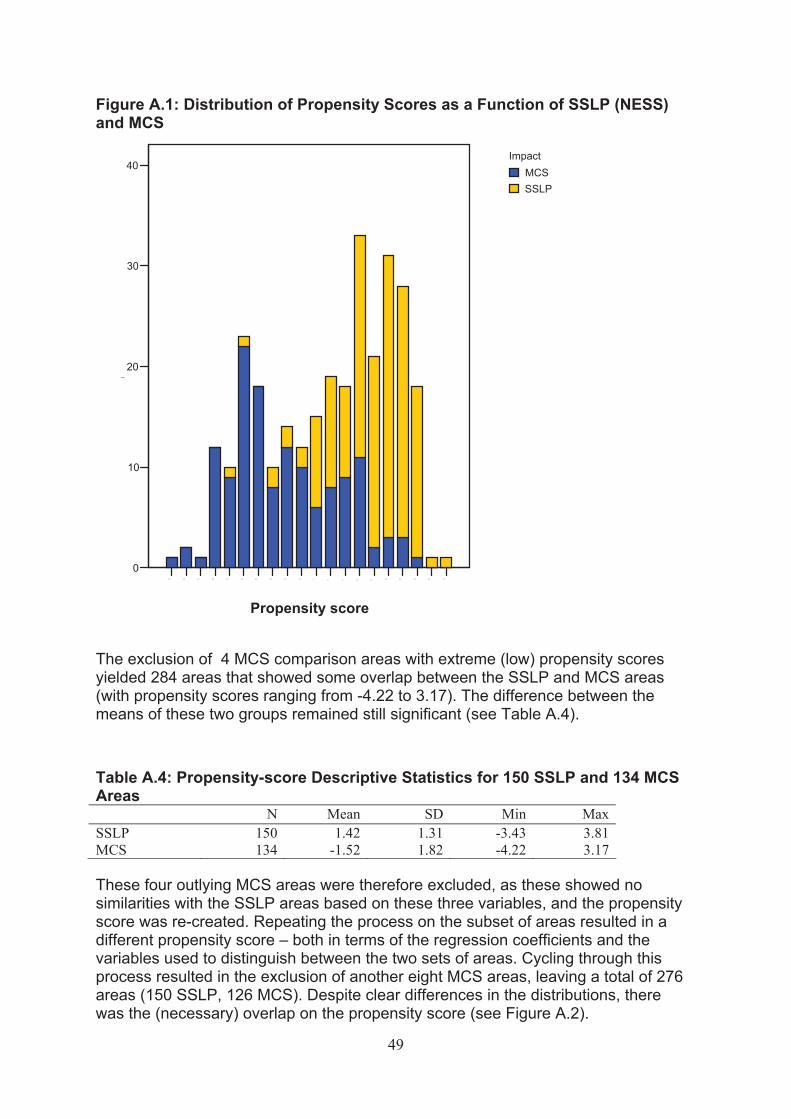
Figure A.1: Distribution of Propensity Scores as a Function of SSLP (NESS) and MCS

SSLPMCS

Impact

Count

40

30

20

10

0

Propensity score

-5.5 -5.0 -4.5 -4.0 -3.5 -3.0 -2.5 4.03.53.02.52.01.51.0.5.0-.5-1.0-1.5-2.0

The exclusion of 4 MCS comparison areas with extreme (low) propensity scores yielded 284 areas that showed some overlap between the SSLP and MCS areas (with propensity scores ranging from -4.22 to 3.17). The difference between the means of these two groups remained still significant (see Table A.4).

Table A.4: Propensity-score Descriptive Statistics for 150 SSLP and 134 MCS Areas

N Mean SD Min MaxSSLP 150 1.42 1.31 -3.43 3.81MCS 134 -1.52 1.82 -4.22 3.17

These four outlying MCS areas were therefore excluded, as these showed no similarities with the SSLP areas based on these three variables, and the propensity score was re-created. Repeating the process on the subset of areas resulted in a different propensity score – both in terms of the regression coefficients and the variables used to distinguish between the two sets of areas. Cycling through this process resulted in the exclusion of another eight MCS areas, leaving a total of 276 areas (150 SSLP, 126 MCS). Despite clear differences in the distributions, there was the (necessary) overlap on the propensity score (see Figure A.2).

49

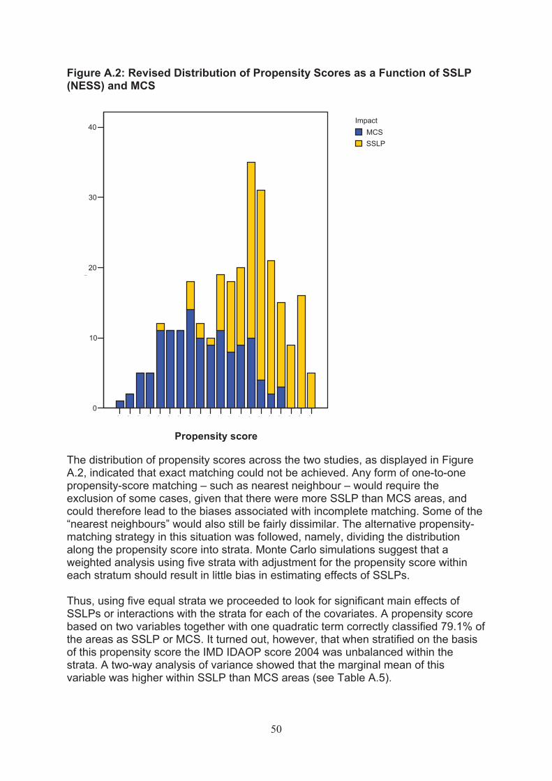
Figure A.2: Revised Distribution of Propensity Scores as a Function of SSLP (NESS) and MCS

The distribution of propensity scores across the two studies, as displayed in Figure A.2, indicated that exact matching could not be achieved. Any form of one-to-one propensity-score matching – such as nearest neighbour – would require the exclusion of some cases, given that there were more SSLP than MCS areas, and could therefore lead to the biases associated with incomplete matching. Some of the “nearest neighbours” would also still be fairly dissimilar. The alternative propensity-matching strategy in this situation was followed, namely, dividing the distribution along the propensity score into strata. Monte Carlo simulations suggest that a weighted analysis using five strata with adjustment for the propensity score within each stratum should result in little bias in estimating effects of SSLPs.

Thus, using five equal strata we proceeded to look for significant main effects of SSLPs or interactions with the strata for each of the covariates. A propensity score based on two variables together with one quadratic term correctly classified 79.1% of the areas as SSLP or MCS. It turned out, however, that when stratified on the basis of this propensity score the IMD IDAOP score 2004 was unbalanced within the strata. A two-way analysis of variance showed that the marginal mean of this variable was higher within SSLP than MCS areas (see Table A.5).

SSLPMCS

Impact

Count

40

30

20

10

0

Propensity score

-5.5 -5.0 -4.5 -4.0 -3.5 -3.0 -2.5 4.03.53.02.52.01.51.0.5.0-.5-1.0-1.5-2.0

50

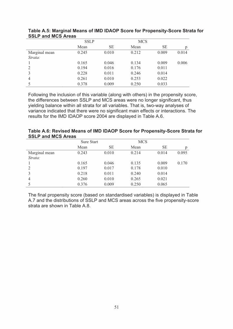
Table A.5: Marginal Means of IMD IDAOP Score for Propensity-Score Strata for SSLP and MCS Areas

SSLP MCS Mean SE Mean SE p

Marginal mean 0.245 0.010 0.212 0.009 0.014 Strata: 1 0.165 0.046 0.134 0.009 0.006 2 0.194 0.016 0.176 0.011 3 0.228 0.011 0.246 0.014 4 0.261 0.010 0.253 0.022 5 0.378 0.009 0.250 0.033

Following the inclusion of this variable (along with others) in the propensity score, the differences between SSLP and MCS areas were no longer significant, thus yielding balance within all strata for all variables. That is, two-way analyses of variance indicated that there were no significant main effects or interactions. The results for the IMD IDAOP score 2004 are displayed in Table A.6.

Table A.6: Revised Means of IMD IDAOP Score for Propensity-Score Strata for SSLP and MCS Areas

Sure Start MCS Mean SE Mean SE p

Marginal mean 0.243 0.010 0.214 0.014 0.095 Strata: 1 0.165 0.046 0.135 0.009 0.170 2 0.197 0.017 0.178 0.010 3 0.218 0.011 0.240 0.014 4 0.260 0.010 0.265 0.021 5 0.376 0.009 0.250 0.065

The final propensity score (based on standardised variables) is displayed in Table A.7 and the distributions of SSLP and MCS areas across the five propensity-score strata are shown in Table A.8.

51

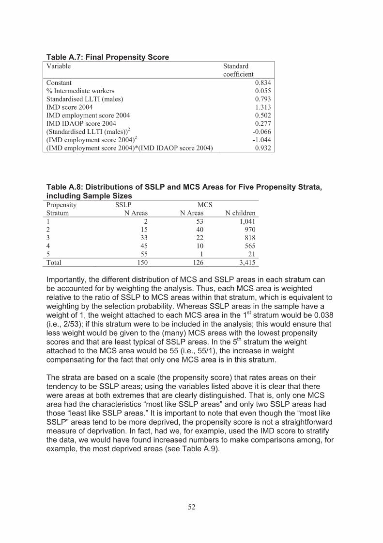
Table A.7: Final Propensity Score Variable Standard

coefficient Constant % Intermediate workers Standardised LLTI (males) IMD score 2004 IMD employment score 2004 IMD IDAOP score 2004 (Standardised LLTI (males))2

(IMD employment score 2004)2

(IMD employment score 2004)*(IMD IDAOP score 2004)

0.834 0.055 0.793 1.313 0.502 0.277

-0.066 -1.044 0.932

�

Table A.8: Distributions of SSLP and MCS Areas for Five Propensity Strata, including Sample Sizes Propensity SSLP MCS Stratum N Areas N Areas N children 1 2 53 1,041 2 15 40 970 3 33 22 818 4 45 10 565 5 55 1 21 Total 150 126 3,415

Importantly, the different distribution of MCS and SSLP areas in each stratum can be accounted for by weighting the analysis. Thus, each MCS area is weighted relative to the ratio of SSLP to MCS areas within that stratum, which is equivalent to weighting by the selection probability. Whereas SSLP areas in the sample have a weight of 1, the weight attached to each MCS area in the 1st stratum would be 0.038 (i.e., 2/53); if this stratum were to be included in the analysis; this would ensure that less weight would be given to the (many) MCS areas with the lowest propensity scores and that are least typical of SSLP areas. In the 5th stratum the weight attached to the MCS area would be 55 (i.e., 55/1), the increase in weight compensating for the fact that only one MCS area is in this stratum.

The strata are based on a scale (the propensity score) that rates areas on their tendency to be SSLP areas; using the variables listed above it is clear that there were areas at both extremes that are clearly distinguished. That is, only one MCS area had the characteristics “most like SSLP areas” and only two SSLP areas had those “least like SSLP areas.” It is important to note that even though the “most like SSLP” areas tend to be more deprived, the propensity score is not a straightforward measure of deprivation. In fact, had we, for example, used the IMD score to stratify the data, we would have found increased numbers to make comparisons among, for example, the most deprived areas (see Table A.9).

52

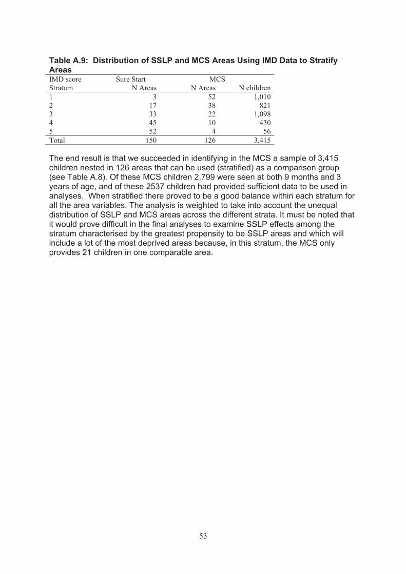
Table A.9: Distribution of SSLP and MCS Areas Using IMD Data to Stratify Areas IMD score Sure Start MCS Stratum N Areas N Areas N children 1 3 52 1,010 2 17 38 821 3 33 22 1,098 4 45 10 430 5 52 4 56 Total 150 126 3,415

The end result is that we succeeded in identifying in the MCS a sample of 3,415 children nested in 126 areas that can be used (stratified) as a comparison group (see Table A.8). Of these MCS children 2,799 were seen at both 9 months and 3 years of age, and of these 2537 children had provided sufficient data to be used in analyses. When stratified there proved to be a good balance within each stratum for all the area variables. The analysis is weighted to take into account the unequal distribution of SSLP and MCS areas across the different strata. It must be noted that it would prove difficult in the final analyses to examine SSLP effects among the stratum characterised by the greatest propensity to be SSLP areas and which will include a lot of the most deprived areas because, in this stratum, the MCS only provides 21 children in one comparable area.

53

Appendix B: Comparison of Children/Families Seen and Not Seen at 5 years.

In the following tables of Appendix B the distribution of characteristics for the sample seen at 5 years is given in the first (left) part of the table; the characteristics of the sample not seen at 5 years (attrition) is given in the middle column; and the results of tests of the differences between those seen and not seen at 5 years are given in the right part of the table. Data are broken down by strata 1 to 5. Also the data are presented separately for the NESS (B1) and MCS (B2) samples used in the study.

54

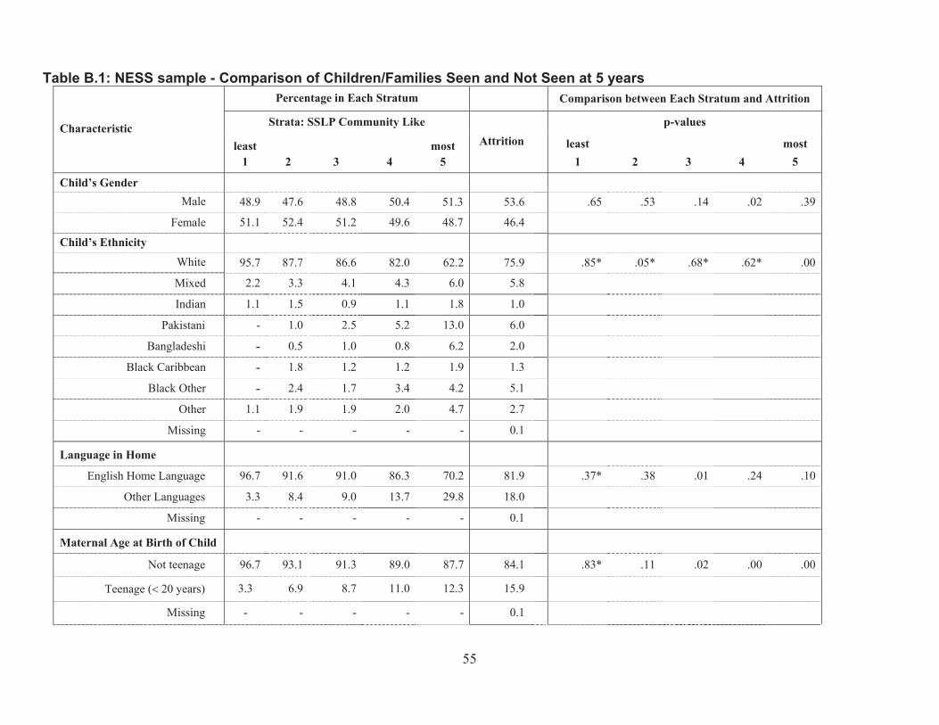
Characteristic

Percentage in Each Stratum Comparison between Each Stratum and Attrition

Strata: SSLP Community Like

least 1 2 3 4

most 5

Attrition p-values

least 1 2 3 4

most 5

Child’s Gender Male

Female

48.9 47.6 48.8 50.4 51.3

51.1 52.4 51.2 49.6 48.7

53.6

46.4

.65 .53 .14 .02 .39

Child’s Ethnicity

White

Mixed

Indian

Pakistani

Bangladeshi

Black Caribbean

Black Other

Other

Missing

95.7 87.7 86.6 82.0 62.2

2.2 3.3 4.1 4.3 6.0

1.1 1.5 0.9 1.1 1.8

- 1.0 2.5 5.2 13.0

- 0.5 1.0 0.8 6.2

- 1.8 1.2 1.2 1.9

- 2.4 1.7 3.4 4.2

1.1 1.9 1.9 2.0 4.7

- - - - -

75.9

5.8

1.0

6.0

2.0

1.3

5.1

2.7

0.1

.85* .05* .68* .62* .00

Language in Home

English Home Language 96.7 91.6 91.0 86.3 70.2 81.9 .37* .38 .01 .24 .10

Other Languages 3.3 8.4 9.0 13.7 29.8 18.0

Missing - - - - - 0.1

Maternal Age at Birth of Child

Not teenage 96.7 93.1 91.3 89.0 87.7 84.1 .83* .11 .02 .00 .00

Teenage (� 20 years) 3.3 6.9 8.7 11.0 12.3 15.9

Missing - - - - - 0.1

Table B.1: NESS sample - Comparison of Children/Families Seen and Not Seen at 5 years

55

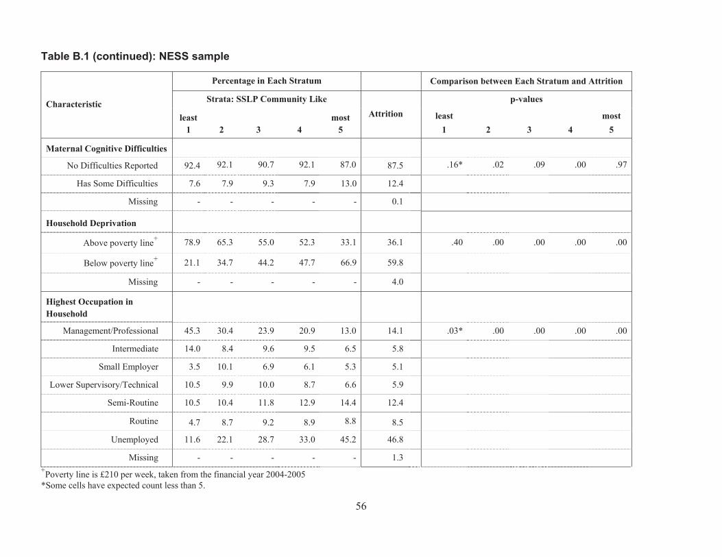
Characteristic

Percentage in Each Stratum Comparison between Each Stratum and Attrition

Strata: SSLP Community Like

least 1 2 3 4

most 5

Attrition p-values

least 1 2 3 4

most 5

Maternal Cognitive Difficulties

No Difficulties Reported

Has Some Difficulties

Missing

92.4 92.1 90.7 92.1 87.0

7.6 7.9 9.3 7.9 13.0

- - - - -

87.5

12.4

0.1

.16* .02 .09 .00 .97

Household Deprivation

Above poverty line+

Below poverty line+

Missing

78.9 65.3 55.0 52.3 33.1

21.1 34.7 44.2 47.7 66.9

- - - - -

36.1

59.8

4.0

.40 .00 .00 .00 .00

Highest Occupation in Household

Management/Professional 45.3 30.4 23.9 20.9 13.0 14.1 .03* .00 .00 .00 .00

Intermediate 14.0 8.4 9.6 9.5 6.5 5.8

Small Employer 3.5 10.1 6.9 6.1 5.3 5.1

Lower Supervisory/Technical 10.5 9.9 10.0 8.7 6.6 5.9

Semi-Routine 10.5 10.4 11.8 12.9 14.4 12.4

Routine 4.7 8.7 9.2 8.9 8.8 8.5

Unemployed 11.6 22.1 28.7 33.0 45.2 46.8

Missing - - - - - 1.3

Table B.1 (continued): NESS sample

+Poverty line is £210 per week, taken from the financial year 2004-2005 *Some cells have expected count less than 5.

56

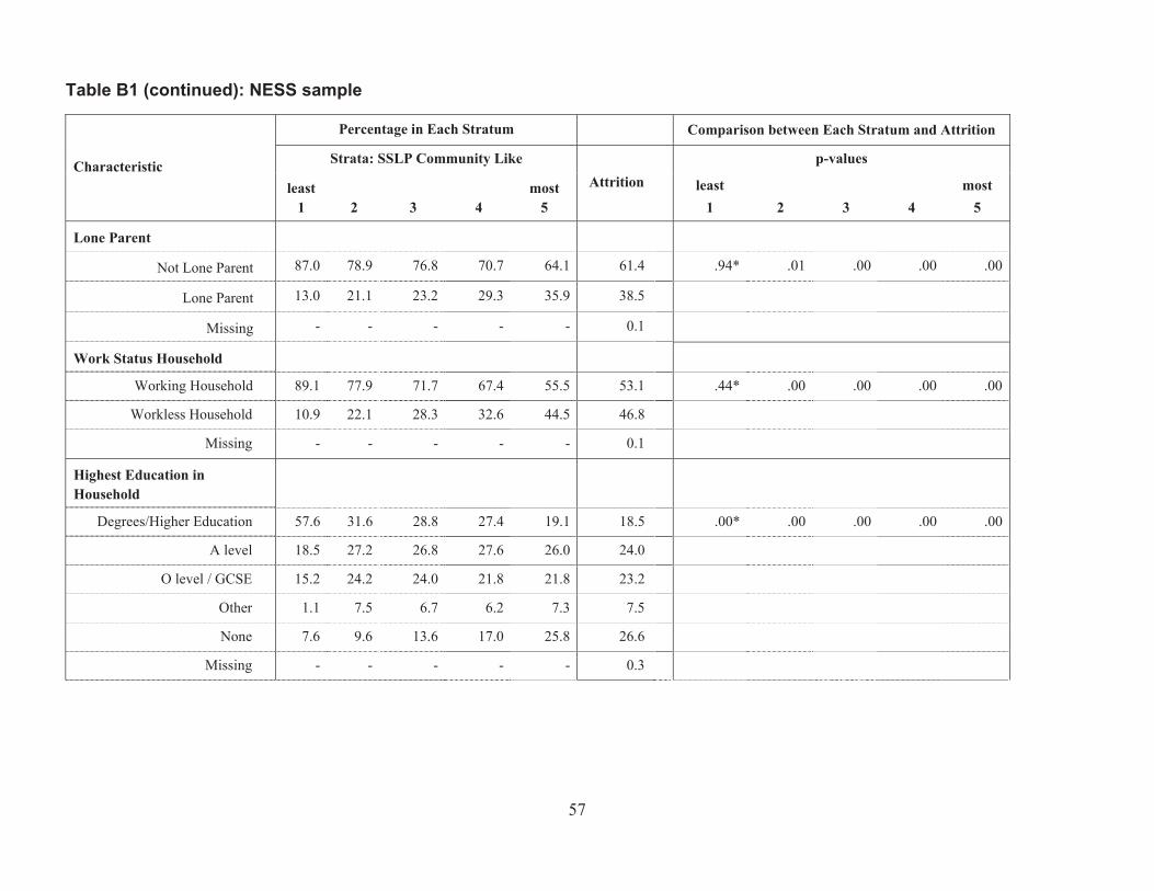
Characteristic

Percentage in Each Stratum Comparison between Each Stratum and Attrition

Strata: SSLP Community Like

least 1 2 3 4

most 5

Attrition p-values

least 1 2 3 4

most 5

Lone Parent

Not Lone Parent

Lone Parent

Missing

87.0 78.9 76.8 70.7 64.1

13.0 21.1 23.2 29.3 35.9

- - - - -

61.4

38.5

0.1

.94* .01 .00 .00 .00

Work Status Household

Working Household

Workless Household

Missing

89.1 77.9 71.7 67.4 55.5

10.9 22.1 28.3 32.6 44.5

- - - - -

53.1

46.8

0.1

.44* .00 .00 .00 .00

Highest Education in Household

Degrees/Higher Education 57.6 31.6 28.8 27.4 19.1 18.5 .00* .00 .00 .00 .00

A level 18.5 27.2 26.8 27.6 26.0 24.0

O level / GCSE 15.2 24.2 24.0 21.8 21.8 23.2

Other 1.1 7.5 6.7 6.2 7.3 7.5

None 7.6 9.6 13.6 17.0 25.8 26.6

Missing - - - - - 0.3

Table B1 (continued): NESS sample

57

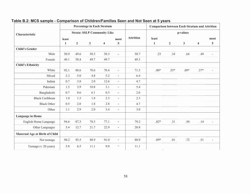
Characteristic

Percentage in Each Stratum Comparison between Each Stratum and Attrition

Strata: SSLP Community Like p-values

least most Attrition least most 1 2 3 4 5 1 2 3 4 5

Child’s Gender Male 50.9 49.6 50.3 50.3 - 50.7 .23 .34 .64 .49 -

Female 49.1 50.4 49.7 49.7 49.3

Child’s Ethnicity

White 92.1 80.6 70.6 70.4 - 71.5 .00* .55* .09* .57* -

Mixed 2.3 5.0 4.8 5.2 - 6.4

Indian 0.7 3.8 2.0 12.6 - 4.7

Pakistani 1.5 3.9 10.8 3.1 - 5.4

Bangladeshi 0.7 0.6 6.1 0.3 - 2.0

Black Caribbean 1.0 1.3 1.8 2.3 - 2.3

Black Other 0.5 2.0 1.8 2.8 - 4.7

Other 1.1 2.9 2.0 3.4 - 3.0

Language in Home

English Home Language 94.6 87.3 78.3 77.1 - 79.2 .02* .31 .50 .14 -

Other Languages 5.4 12.7 21.7 22.9 - 20.8

Maternal Age at Birth of Child

Not teenage 94.2 93.5 88.9 91.0 - 88.9 .89* .01 .72 .51 -

Teenage (� 20 years) 5.8 6.5 11.1 9.0 - 11.1

Table B.2: MCS sample - Comparison of Children/Families Seen and Not Seen at 5 years

58

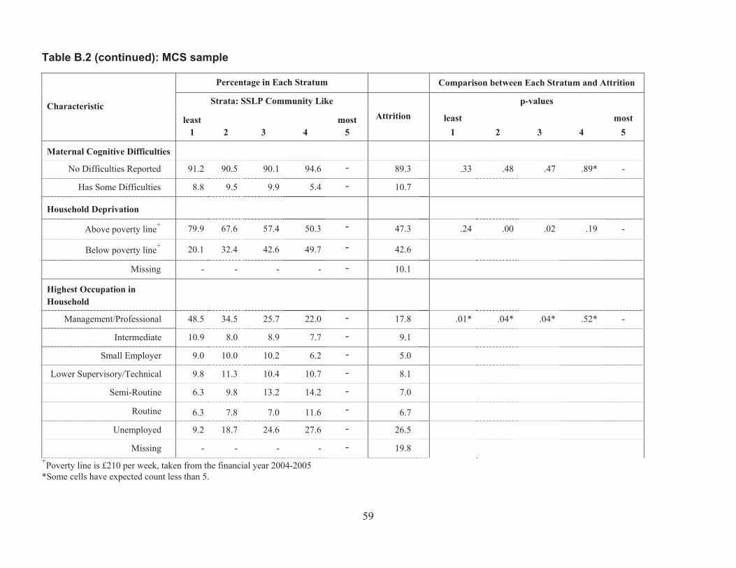
Characteristic

Percentage in Each Stratum Comparison between Each Stratum and Attrition

Strata: SSLP Community Like

least 1 2 3 4

most 5

Attrition p-values

least 1 2 3 4

most 5

Maternal Cognitive Difficulties

No Difficulties Reported

Has Some Difficulties

91.2 90.5 90.1 94.6 -

8.8 9.5 9.9 5.4 -89.3

10.7

.33 .48 .47 .89* -

Household Deprivation

Above poverty line+

Below poverty line+

Missing

79.9 67.6 57.4 50.3 -

20.1 32.4 42.6 49.7 -

- - - - -

47.3

42.6

10.1

.24 .00 .02 .19 -

Highest Occupation in Household

Management/Professional 48.5 34.5 25.7 22.0 - 17.8 .01* .04* .04* .52* -

Intermediate 10.9 8.0 8.9 7.7 - 9.1

Small Employer 9.0 10.0 10.2 6.2 - 5.0

Lower Supervisory/Technical 9.8 11.3 10.4 10.7 - 8.1

Semi-Routine 6.3 9.8 13.2 14.2 - 7.0

Routine 6.3 7.8 7.0 11.6 - 6.7

Unemployed 9.2 18.7 24.6 27.6 - 26.5

Missing - - - - - 19.8

Table B.2 (continued): MCS sample

+Poverty line is £210 per week, taken from the financial year 2004-2005 *Some cells have expected count less than 5.

59

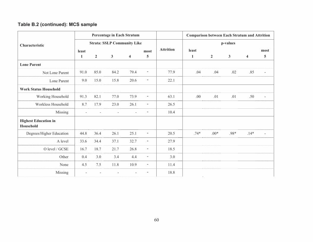
Characteristic

Percentage in Each Stratum Comparison between Each Stratum and Attrition

Strata: SSLP Community Like

least 1 2 3 4

most 5

Attrition p-values

least 1 2 3 4

most 5

Lone Parent

Not Lone Parent

Lone Parent

91.0 85.0 84.2 79.4 -

9.0 15.0 15.8 20.6 -77.9

22.1

.04 .04 .02 .85 -

Work Status Household

Working Household

Workless Household

Missing

91.3 82.1 77.0 73.9 -

8.7 17.9 23.0 26.1 -

- - - - -

63.1

26.5

10.4

.00 .01 .01 .50 -

Highest Education in Household

Degrees/Higher Education 44.8 36.4 26.1 25.1 - 20.5 .74* .00* .98* .14* -

A level 33.6 34.4 37.1 32.7 - 27.9

O level / GCSE 16.7 18.7 21.7 26.8 - 18.5

Other 0.4 3.0 3.4 4.4 - 3.0

None 4.5 7.5 11.8 10.9 - 11.4

Missing - - - - - 18.8

Table B.2 (continued): MCS sample

60

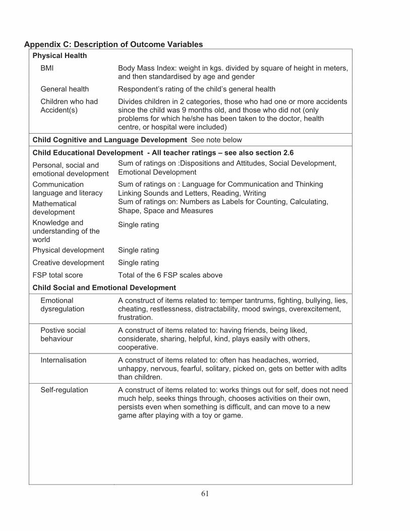
Appendix C: Description of Outcome Variables Physical Health

BMI Body Mass Index: weight in kgs. divided by square of height in meters,and then standardised by age and gender

General health Respondent’s rating of the child’s general health

Children who had Divides children in 2 categories, those who had one or more accidentsAccident(s) since the child was 9 months old, and those who did not (only

problems for which he/she has been taken to the doctor, health centre, or hospital were included)

Child Cognitive and Language Development See note below

Child Educational Development - All teacher ratings – see also section 2.6 Personal, social and Sum of ratings on :Dispositions and Attitudes, Social Development, emotional development Emotional Development Communication Sum of ratings on : Language for Communication and Thinking language and literacy Linking Sounds and Letters, Reading, Writing Mathematical Sum of ratings on: Numbers as Labels for Counting, Calculating, development Shape, Space and Measures Knowledge and Single rating understanding of the world Physical development Single rating

Creative development Single rating

FSP total score Total of the 6 FSP scales above

Child Social and Emotional Development Emotional A construct of items related to: temper tantrums, fighting, bullying, lies, dysregulation cheating, restlessness, distractability, mood swings, overexcitement,

frustration.

Postive social A construct of items related to: having friends, being liked, behaviour considerate, sharing, helpful, kind, plays easily with others,

cooperative.

Internalisation A construct of items related to: often has headaches, worried, unhappy, nervous, fearful, solitary, picked on, gets on better with adlts than children.

Self-regulation A construct of items related to: works things out for self, does not need much help, seeks things through, chooses activities on their own, persists even when something is difficult, and can move to a new game after playing with a toy or game.

61

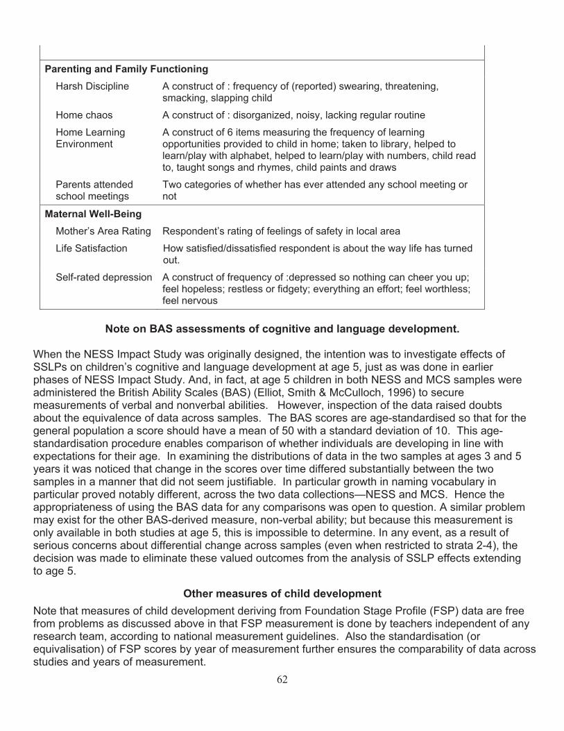
Parenting and Family F Harsh Discipline

Home chaos

Home Learning Environment

Parents attended school meetings

unctioning A construct of : frequency of (reported) swearing, threatening, smacking, slapping child

A construct of : disorganized, noisy, lacking regular routine

A construct of 6 items measuring the frequency of learning opportunities provided to child in home; taken to library, helped to learn/play with alphabet, helped to learn/play with numbers, child read to, taught songs and rhymes, child paints and draws

Two categories of whether has ever attended any school meeting or not

Maternal Well-Being Mother’s Area Rating

Life Satisfaction

Self-rated depression

Respondent’s rating of feelings of safety in local area

How satisfied/dissatisfied respondent is about the way life has turned out.

A construct of frequency of :depressed so nothing can cheer you up; feel hopeless; restless or fidgety; everything an effort; feel worthless; feel nervous

Note on BAS assessments of cognitive and language development.

When the NESS Impact Study was originally designed, the intention was to investigate effects of SSLPs on children’s cognitive and language development at age 5, just as was done in earlier phases of NESS Impact Study. And, in fact, at age 5 children in both NESS and MCS samples were administered the British Ability Scales (BAS) (Elliot, Smith & McCulloch, 1996) to secure measurements of verbal and nonverbal abilities. However, inspection of the data raised doubts about the equivalence of data across samples. The BAS scores are age-standardised so that for the general population a score should have a mean of 50 with a standard deviation of 10. This age-standardisation procedure enables comparison of whether individuals are developing in line with expectations for their age. In examining the distributions of data in the two samples at ages 3 and 5 years it was noticed that change in the scores over time differed substantially between the two samples in a manner that did not seem justifiable. In particular growth in naming vocabulary in particular proved notably different, across the two data collections—NESS and MCS. Hence the appropriateness of using the BAS data for any comparisons was open to question. A similar problem may exist for the other BAS-derived measure, non-verbal ability; but because this measurement is only available in both studies at age 5, this is impossible to determine. In any event, as a result of serious concerns about differential change across samples (even when restricted to strata 2-4), the decision was made to eliminate these valued outcomes from the analysis of SSLP effects extending to age 5.

Other measures of child development Note that measures of child development deriving from Foundation Stage Profile (FSP) data are free from problems as discussed above in that FSP measurement is done by teachers independent of any research team, according to national measurement guidelines. Also the standardisation (or equivalisation) of FSP scores by year of measurement further ensures the comparability of data across studies and years of measurement.

62

Appendix D: Imputation procedure

There is a strategy to overcome the problem that data may be missing in non-random ways and hence bias results. This involves the “imputation” of missing data. Imputation is based on the fundamental premise that tolerably accurate estimates of what a missing value would have been had the information been supplied can be determined using all the data that has been collected. Taking an over-simplified example, knowing a person’s age, education level, gender, work status and occupation enables a reasonably accurate prediction of salary, should salary data be missing, using data on all these variables obtained from respondents who also provided salary information. In the current evaluation, statistically sophisticated and widely used multiple-imputation techniques were employed to overcome the possibility of bias in results caused by non-random missing data. This takes into account that, in the above example, we can predict not just one value for the missing salary but a range of plausible values.

Two approaches have been taken for dealing with missing data: case deletion and imputation. Case deletion involves deleting for each outcome measure any individual who has missing data either for the outcome measure or for the demographic or family background characteristics, leaving only cases with complete data. Analysis of data with only complete cases has the drawback that, where we are considering a number of explanatory factors, we may discard quite a large part of the data. Not only is this inefficient, it may result in a subset of data that is small and, if data are missing in a non-random way (i.e. if certain subgroups are more likely to refuse to answer or skip over certain questions), may be unrepresentative of the population as a whole. Imputation of data for a respondent involves filling in the missing values with plausible values based on the known characteristics of that respondent together with the relationship between characteristics observed in the rest of the sample.

Multiple imputation (Rubin, 1987; Schafer, 1997) was used to estimate missing data values using the statistical package IVEware (http://www.isr.umich.edu/src/smp/ive/). Multiple imputation is the process of generating several data sets, analysing these and combining the results. This ensures that we have sufficient variability between imputed values to be able to draw correct inferences. The missing demographic and outcome data were imputed simultaneously for both waves of data. In each strata, the missing data were imputed separately for each study group. Fixed area effects were included to take account of the hierarchical structure of the data. For all the demographic and outcome variables included in the analysis of strata 2-4, 3.6% of the data were missing in the dataset. Table D.1 show the percent missing for each of the demographic and family background characteristic variables by strata and study, for those strata used in the analyses, and also for strata 2-4 by study. Table D.2 shows for each outcome measure the percent of cases with missing outcome measures and incomplete data (missing outcome and/or missing demographic or family background characteristics). For the complete-cases data analysis, the incomplete-data cases are excluded. For the 9-month data, between 8% and 14% of the cases are excluded from any one analysis. For the 3-year data, higher rates of missing data were observed, between 10% and 29% of the cases.

Rubin, D.B. (1987) Multiple Imputation for Nonresponse in Surveys. London: Wiley. Schafer, J.L. (1997) Analysis of Incomplete Multivariate Data. London: Chapman & Hall.

63

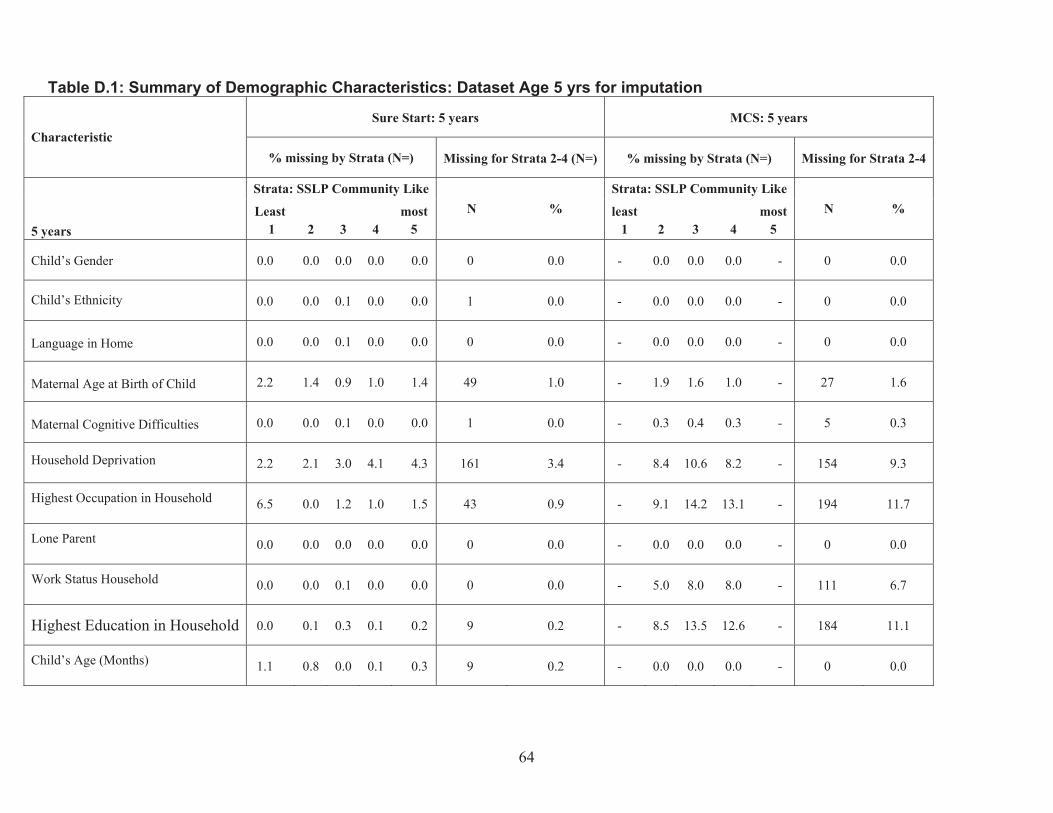
Table D.1: Summary of Demographic Characteristics: Dataset Age 5 yrs for imputation

Characteristic Sure Start: 5 years MCS: 5 years

% missing by Strata (N=) Missing for Strata 2-4 (N=) % missing by Strata (N=) Missing for Strata 2-4

5 years

Strata: SSLP Community Like

Least 1 2 3 4

most 5

N % Strata: SSLP Community Like

least 1 2 3 4

most 5

N %

Child’s Gender 0.0 0.0 0.0 0.0 0.0 0 0.0 - 0.0 0.0 0.0 - 0 0.0

Child’s Ethnicity 0.0 0.0 0.1 0.0 0.0 1 0.0 - 0.0 0.0 0.0 - 0 0.0

Language in Home 0.0 0.0 0.1 0.0 0.0 0 0.0 - 0.0 0.0 0.0 - 0 0.0

Maternal Age at Birth of Child 2.2 1.4 0.9 1.0 1.4 49 1.0 - 1.9 1.6 1.0 - 27 1.6

Maternal Cognitive Difficulties 0.0 0.0 0.1 0.0 0.0 1 0.0 - 0.3 0.4 0.3 - 5 0.3

Household Deprivation 2.2 2.1 3.0 4.1 4.3 161 3.4 - 8.4 10.6 8.2 - 154 9.3

Highest Occupation in Household 6.5 0.0 1.2 1.0 1.5 43 0.9 - 9.1 14.2 13.1 - 194 11.7

Lone Parent 0.0 0.0 0.0 0.0 0.0 0 0.0 - 0.0 0.0 0.0 - 0 0.0

Work Status Household 0.0 0.0 0.1 0.0 0.0 0 0.0 - 5.0 8.0 8.0 - 111 6.7

Highest Education in Household 0.0 0.1 0.3 0.1 0.2 9 0.2 - 8.5 13.5 12.6 - 184 11.1

Child’s Age (Months) 1.1 0.8 0.0 0.1 0.3 9 0.2 - 0.0 0.0 0.0 - 0 0.0

64

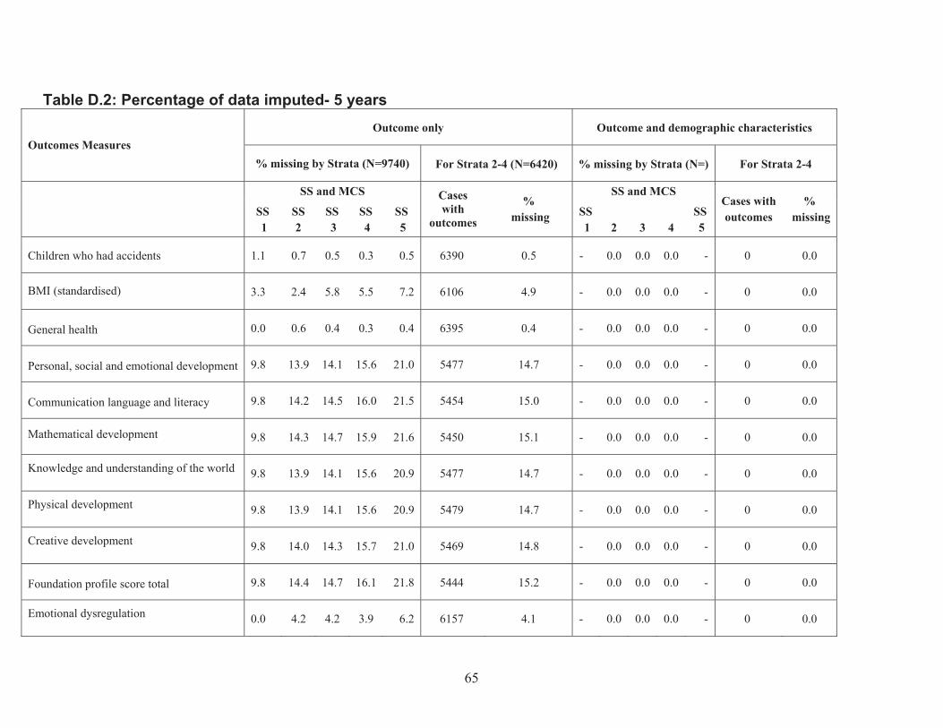
Table D.2: Percentage of data imputed- 5 years

Outcomes Measures Outcome only Outcome and demographic characteristics

% missing by Strata (N=9740) For Strata 2-4 (N=6420) % missing by Strata (N=) For Strata 2-4

SS and MCS

SS 1

SS 2

SS 3

SS 4

SS 5

Cases with

outcomes

% missing

SS and MCS

SS 1 2 3 4

SS 5

Cases with outcomes

% missing

Children who had accidents 1.1 0.7 0.5 0.3 0.5 6390 0.5 - 0.0 0.0 0.0 - 0 0.0

BMI (standardised) 3.3 2.4 5.8 5.5 7.2 6106 4.9 - 0.0 0.0 0.0 - 0 0.0

General health 0.0 0.6 0.4 0.3 0.4 6395 0.4 - 0.0 0.0 0.0 - 0 0.0

Personal, social and emotional development 9.8 13.9 14.1 15.6 21.0 5477 14.7 - 0.0 0.0 0.0 - 0 0.0

Communication language and literacy 9.8 14.2 14.5 16.0 21.5 5454 15.0 - 0.0 0.0 0.0 - 0 0.0

Mathematical development 9.8 14.3 14.7 15.9 21.6 5450 15.1 - 0.0 0.0 0.0 - 0 0.0

Knowledge and understanding of the world 9.8 13.9 14.1 15.6 20.9 5477 14.7 - 0.0 0.0 0.0 - 0 0.0

Physical development 9.8 13.9 14.1 15.6 20.9 5479 14.7 - 0.0 0.0 0.0 - 0 0.0

Creative development 9.8 14.0 14.3 15.7 21.0 5469 14.8 - 0.0 0.0 0.0 - 0 0.0

Foundation profile score total 9.8 14.4 14.7 16.1 21.8 5444 15.2 - 0.0 0.0 0.0 - 0 0.0

Emotional dysregulation 0.0 4.2 4.2 3.9 6.2 6157 4.1 - 0.0 0.0 0.0 - 0 0.0

65

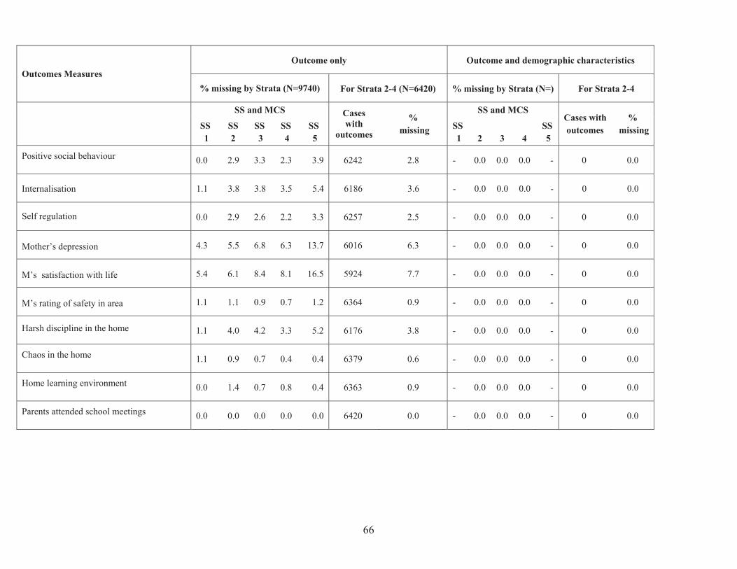
Outcomes Measures Outcome only Outcome and demographic characteristics

% missing by Strata (N=9740) For Strata 2-4 (N=6420) % missing by Strata (N=) For Strata 2-4

SS and MCS

SS 1

SS 2

SS 3

SS 4

SS 5

Cases with

outcomes

% missing

SS and MCS

SS 1 2 3 4

SS 5

Cases with outcomes

% missing

Positive social behaviour 0.0 2.9 3.3 2.3 3.9 6242 2.8 - 0.0 0.0 0.0 - 0 0.0

Internalisation 1.1 3.8 3.8 3.5 5.4 6186 3.6 - 0.0 0.0 0.0 - 0 0.0

Self regulation 0.0 2.9 2.6 2.2 3.3 6257 2.5 - 0.0 0.0 0.0 - 0 0.0

Mother’s depression 4.3 5.5 6.8 6.3 13.7 6016 6.3 - 0.0 0.0 0.0 - 0 0.0

M’s satisfaction with life 5.4 6.1 8.4 8.1 16.5 5924 7.7 - 0.0 0.0 0.0 - 0 0.0

M’s rating of safety in area 1.1 1.1 0.9 0.7 1.2 6364 0.9 - 0.0 0.0 0.0 - 0 0.0

Harsh discipline in the home 1.1 4.0 4.2 3.3 5.2 6176 3.8 - 0.0 0.0 0.0 - 0 0.0

Chaos in the home 1.1 0.9 0.7 0.4 0.4 6379 0.6 - 0.0 0.0 0.0 - 0 0.0

Home learning environment 0.0 1.4 0.7 0.8 0.4 6363 0.9 - 0.0 0.0 0.0 - 0 0.0

Parents attended school meetings 0.0 0.0 0.0 0.0 0.0 6420 0.0 - 0.0 0.0 0.0 - 0 0.0

66

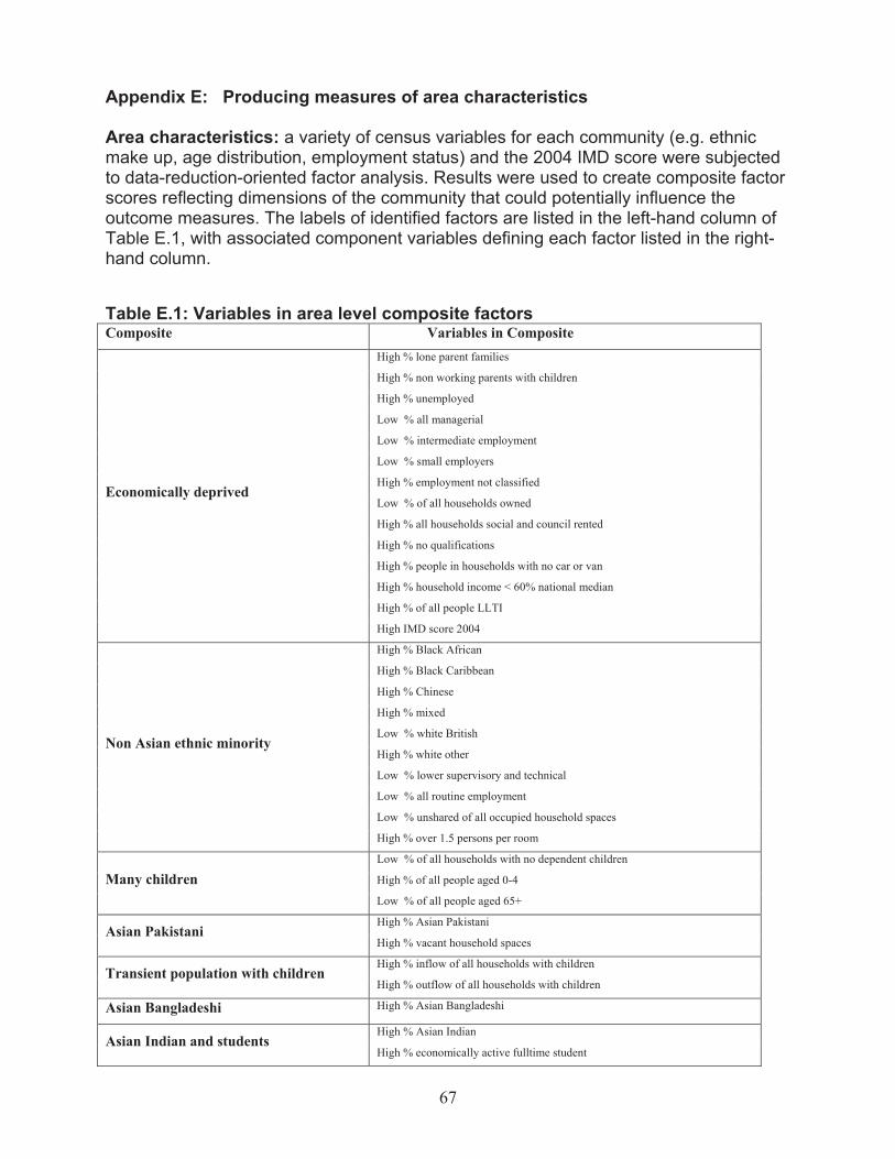
Appendix E: Producing measures of area characteristics

Area characteristics: a variety of census variables for each community (e.g. ethnic make up, age distribution, employment status) and the 2004 IMD score were subjected to data-reduction-oriented factor analysis. Results were used to create composite factor scores reflecting dimensions of the community that could potentially influence the outcome measures. The labels of identified factors are listed in the left-hand column of Table E.1, with associated component variables defining each factor listed in the right-hand column.

Table E.1: Variables in area level composite factors Composite Variables in Composite

Economically deprived

High % lone parent families

High % non working parents with children

High % unemployed

Low % all managerial

Low % intermediate employment

Low % small employers

High % employment not classified

Low % of all households owned

High % all households social and council rented

High % no qualifications

High % people in households with no car or van

High % household income < 60% national median

High % of all people LLTI

High IMD score 2004

Non Asian ethnic minority

High % Black African

High % Black Caribbean

High % Chinese

High % mixed

Low % white British

High % white other

Low % lower supervisory and technical

Low % all routine employment

Low % unshared of all occupied household spaces

High % over 1.5 persons per room

Many children Low % of all households with no dependent children

High % of all people aged 0-4

Low % of all people aged 65+

Asian Pakistani High % Asian Pakistani

High % vacant household spaces

Transient population with children High % inflow of all households with children

High % outflow of all households with children

Asian Bangladeshi High % Asian Bangladeshi

Asian Indian and students High % Asian Indian

High % economically active fulltime student

67

Appendix F: Effects of Strata and Covariates on Outcomes

In the results section the results of the multilevel models that tested for statistically significant effects upon outcomes are discussed primarily in terms of the main questions related to SSLP versus non-SSLP (MCS) differences. In analysing for such differences a large number of covariates (other predictor variables) were included in the multilevel models, so that SSLP effects could be determined after controlling for covariate differences. In the following tables of Appendix F, the effects of the covariates used in the multilevel models for each outcome are presented. A blank indicates no significant effect, -ve indicates a statistically significant (p<.05) negative effect (as covariate increases - outcome decreases) and +ve indicates a a statistically significant (p<.05) positive effect (as covariate increases - outcome increases).

Results are presented firstly for analyses of the complete cases (F1), secondly for imputed data for all seen at 5 years (F2), and thirdly for imputed data for all seen at 3 years (F3).

68

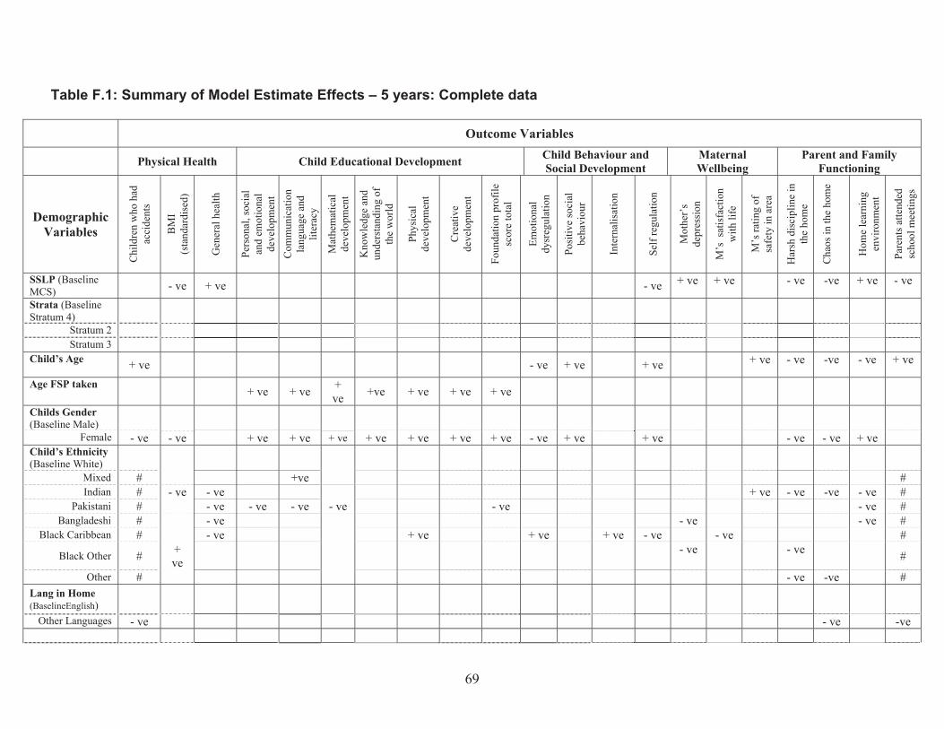
Outcome Variables

Physical Health Child Educational Development Child Behaviour and Social Development

Maternal Wellbeing

Parent and Family Functioning

Demographic Variables

Chi

ldre

n w

ho h

ad

acci

dent

s

BM

I(s

tand

ardi

sed)

Gen

eral

hea

lth

Pers

onal

, soc

ial

and

emot

iona

l de

velo

pmen

t C

omm

unic

atio

nla

ngua

ge a

nd

liter

acy

Mat

hem

atic

alde

velo

pmen

t

Kno

wle

dge

and

unde

rsta

ndin

g of

the

wor

ld

Phys

ical

deve

lopm

ent

Cre

ativ

e de

velo

pmen

t

Foun

datio

n pr

ofile

sc

ore

tota

l

Emot

iona

ldy

sreg

ulat

ion

Posi

tive

soci

albe

havi

our

Inte

rnal

isat

ion

Self

regu

latio

n

Mot

her’

sde

pres

sion

M’s

sat

isfa

ctio

nw

ith li

fe

M’s

ratin

g of

safe

ty in

are

a

Har

sh d

isci

plin

e in

th

e ho

me

Cha

os in

the

hom

e

Hom

e le

arni

ngen

viro

nmen

t

Pare

nts a

ttend

edsc

hool

mee

tings

SSLP (Baseline MCS) - ve + ve - ve + ve + ve - ve -ve + ve - ve

Strata (Baseline Stratum 4)

Stratum 2 Stratum 3

Child’s Age + ve - ve + ve + ve + ve - ve -ve - ve + ve

Age FSP taken + ve + ve +

ve +ve + ve + ve + ve

Childs Gender (Baseline Male)

Female - ve - ve + ve + ve + ve + ve + ve + ve + ve - ve + ve + ve - ve - ve + ve Child’s Ethnicity (Baseline White)

Mixed Indian

Pakistani Bangladeshi

Black Caribbean

Black Other

Other

# # # # #

#

#

- ve

+ ve

- ve - ve - ve - ve

- ve

+ve

- ve - ve

+ ve

- ve

+ ve + ve - ve - ve

- ve - ve

+ ve - ve

- ve

- ve

-ve

-ve

- ve - ve - ve

# # # # #

#

# Lang in Home (BaselineEnglish)

Other Languages - ve - ve -ve

Table F.1: Summary of Model Estimate Effects – 5 years: Complete data

69

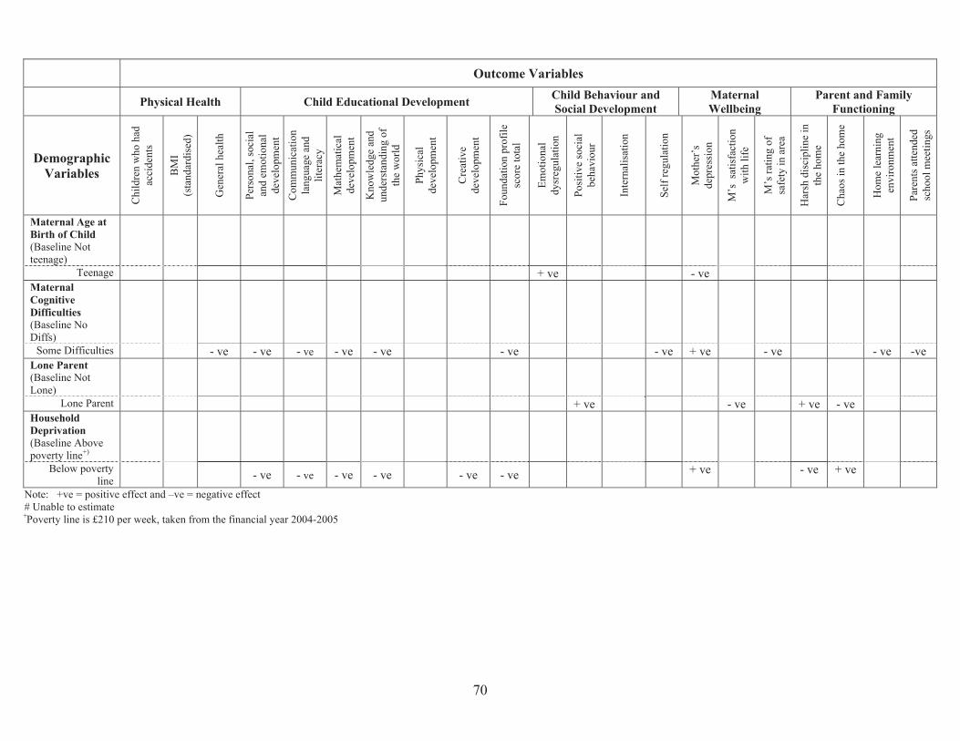
Outcome Variables

Physical Health Child Educational Development Child Behaviour and Social Development

Maternal Wellbeing

Parent and Family Functioning

Demographic Variables

Chi

ldre

n w

ho h

ad

acci

dent

s

BM

I(s

tand

ardi

sed)

Gen

eral

hea

lth

Pers

onal

, soc

ial

and

emot

iona

l de

velo

pmen

t C

omm

unic

atio

nla

ngua

ge a

nd

liter

acy

Mat

hem

atic

alde

velo

pmen

t

Kno

wle

dge

and

unde

rsta

ndin

g of

the

wor

ld

Phys

ical

deve

lopm

ent

Cre

ativ

e de

velo

pmen

t

Foun

datio

n pr

ofile

sc

ore

tota

l

Emot

iona

ldy

sreg

ulat

ion

Posi

tive

soci

albe

havi

our

Inte

rnal

isat

ion

Self

regu

latio

n

Mot

her’

sde

pres

sion

M’s

sat

isfa

ctio

nw

ith li

fe

M’s

ratin

g of

safe

ty in

are

a

Har

sh d

isci

plin

e in

th

e ho

me

Cha

os in

the

hom

e

Hom

e le

arni

ngen

viro

nmen

t

Pare

nts a

ttend

edsc

hool

mee

tings

Maternal Age at Birth of Child (Baseline Not teenage)

Teenage + ve - ve Maternal Cognitive Difficulties (Baseline No Diffs)

Some Difficulties - ve - ve - ve - ve - ve - ve - ve + ve - ve - ve -ve Lone Parent (Baseline Not Lone)

Lone Parent + ve - ve + ve - ve Household Deprivation (Baseline Above poverty line+)

Below poverty line - ve - ve - ve - ve - ve - ve + ve - ve + ve

Note: +ve = positive effect and –ve = negative effect # Unable to estimate

+Poverty line is £210 per week, taken from the financial year 2004-2005

70

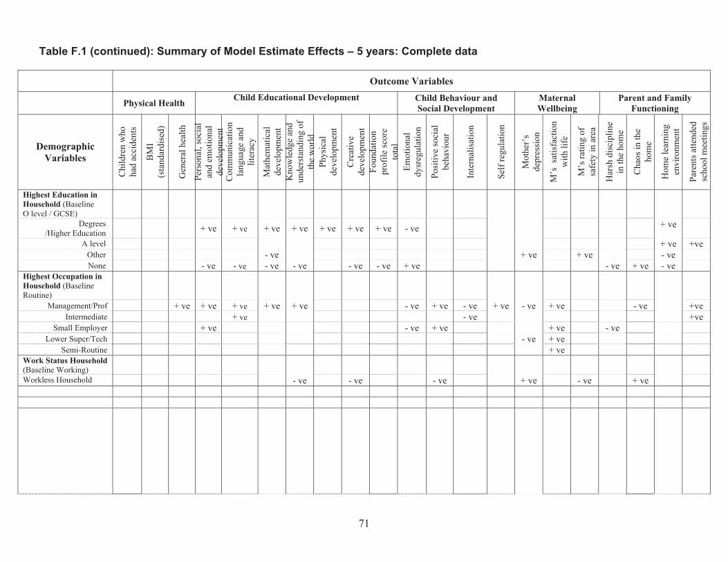
Table F.1 (continued): Summary of Model Estimate Effects – 5 years: Complete data

Outcome Variables

Physical Health Child Educational Development Child Behaviour and Social Development

Maternal Wellbeing

Parent and Family Functioning

Demographic Variables

Chi

ldre

n w

ho

had

acci

dent

s

BM

I(s

tand

ardi

sed)

Gen

eral

hea

lth

Pers

onal

, soc

ial

and

emot

iona

lde

velo

pmen

tC

omm

unic

atio

nla

ngua

ge a

nd

liter

acy

Mat

hem

atic

alde

velo

pmen

tK

now

ledg

e an

dun

ders

tand

ing

ofth

e w

orld

Phys

ical

deve

lopm

ent

Cre

ativ

ede

velo

pmen

tFo

unda

tion

prof

ile sc

ore

tota

lEm

otio

nal

dysr

egul

atio

n

Posi

tive

soci

albe

havi

our

Inte

rnal

isat

ion

Self

regu

latio

n

Mot

her’

s de

pres

sion

M’s

sat

isfa

ctio

n w

ith li

fe

M’s

ratin

g of

sa

fety

in a

rea

Har

sh d

isci

plin

ein

the

hom

e

Cha

os in

the

hom

e

Hom

e le

arni

ngen

viro

nmen

t

Pare

nts a

ttend

edsc

hool

mee

tings

Highest Education in Household (Baseline O level / GCSE)

Degrees /Higher Education

A level Other None

+ ve

- ve

+ ve

- ve

+ ve

- ve - ve

+ ve

- ve

+ ve + ve

- ve

+ ve

- ve

- ve

+ ve + ve + ve

- ve + ve

+ ve

+ ve - ve - ve

+ve

Highest Occupation in Household (Baseline Routine)

Management/Prof Intermediate

Small Employer Lower Super/Tech

Semi-Routine

+ ve + ve

+ ve

+ ve + ve

+ ve + ve - ve

- ve

+ ve

+ ve

- ve - ve

+ ve - ve

- ve

+ ve

+ ve + ve + ve

- ve

- ve +ve +ve

Work Status Household (Baseline Working) Workless Household - ve - ve - ve + ve - ve + ve

71

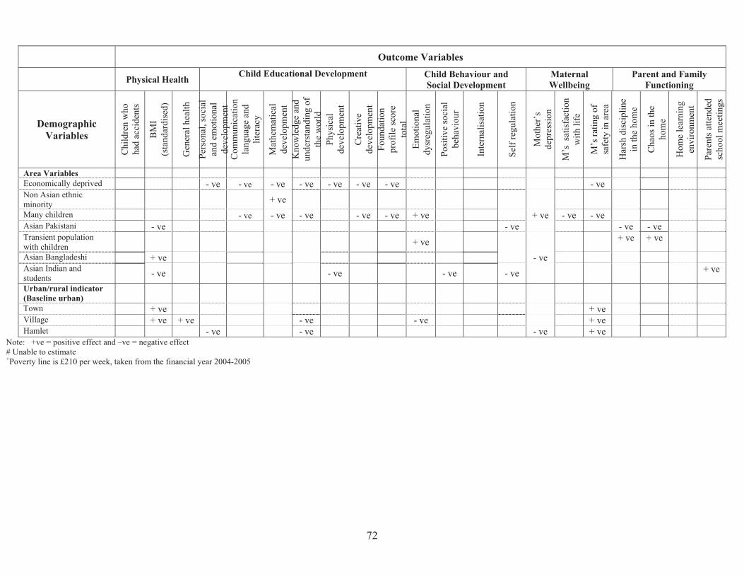
Outcome Variables

Physical Health Child Educational Development Child Behaviour and Social Development

Maternal Wellbeing

Parent and Family Functioning

Demographic Variables

Chi

ldre

n w

ho

had

acci

dent

s

BM

I(s

tand

ardi

sed)

Gen

eral

hea

lth

Pers

onal

, soc

ial

and

emot

iona

lde

velo

pmen

tC

omm

unic

atio

nla

ngua

ge a

nd

liter

acy

Mat

hem

atic

alde

velo

pmen

tK

now

ledg

e an

dun

ders

tand

ing

ofth

e w

orld

Phys

ical

deve

lopm

ent

Cre

ativ

ede

velo

pmen

tFo

un a

tid

onpr

ofile

scor

eto

tal

Emot

iona

ldy

sreg

ulat

ion

Posi

tive

soci

albe

havi

our

Inte

rnal

isat

ion

Self

regu

latio

n

Mot

her’

s de

pres

sion

M’s

sat

isfa

ctio

n w

ith li

fe

M’s

ratin

g of

sa

fety

in a

rea

Har

sh d

isci

plin

ein

the

hom

e

Cha

os in

the

hom

e

Hom

e le

arni

ngen

viro

nmen

t

Pare

nts a

ttend

edsc

hool

mee

tings

Area Variables Economically deprived - ve - ve - ve - ve - ve - ve - ve - ve Non Asian ethnic minority + ve Many children - ve - ve - ve - ve - ve + ve + ve - ve - ve Asian Pakistani - ve - ve - ve - ve Transient population with children + ve + ve + ve

Asian Bangladeshi + ve - ve Asian Indian and students - ve - ve - ve - ve + ve

Urban/rural indicator (Baseline urban) Town Village Hamlet

+ ve + ve + ve

- ve - ve - ve

- ve - ve

+ ve + ve + ve

Note: +ve = positive effect and –ve = negative effect

# Unable to estimate +Poverty line is £210 per week, taken from the financial year 2004-2005

72

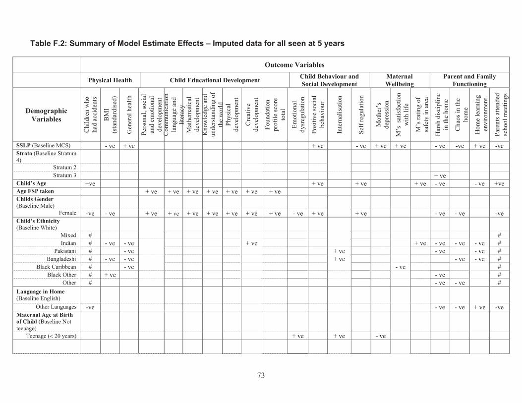
Table F.2: Summary of Model Estimate Effects – Imputed data for all seen at 5 years

Outcome Variables

Physical Health Child Educational Development Child Behaviour and Social Development

Maternal Wellbeing

Parent and Family Functioning

Demographic Variables

Chi

ldre

n w

ho

had

acci

dent

s

BM

I(s

tand

ardi

sed)

Gen

eral

hea

lth

Pers

onal

, soc

ial

and

emot

iona

lde

velo

pmen

tC

omm

unic

atio

nla

ngua

ge a

nd

liter

acy

Mat

hem

atic

alde

velo

pmen

tK

now

ledg

e an

dun

ders

tand

ing

ofth

e w

orld

Phys

ical

deve

lopm

ent

Cre

ativ

ede

velo

pmen

t

Foun

datio

npr

ofile

scor

eto

tal

Emot

iona

ldy

sreg

ulat

ion

Posi

tive

soci

albe

havi

our

Inte

rnal

isat

ion

Self

regu

latio

n

Mot

her’

s de

pres

sion

M’s

sat

isfa

ctio

n w

ith li

fe

M’s

ratin

g of

sa

fety

in a

rea

Har

sh d

isci

plin

ein

the

hom

e

Cha

os in

the

hom

e

Hom

e le

arni

ngen

viro

nmen

t

Pare

nts a

ttend

edsc

hool

mee

tings

SSLP (Baseline MCS) - ve + ve + ve - ve + ve + ve - ve -ve + ve -ve Strata (Baseline Stratum 4)

Stratum 2 Stratum 3 + ve

Child’s Age +ve + ve + ve + ve - ve - ve +ve Age FSP taken + ve + ve + ve + ve + ve + ve + ve Childs Gender (Baseline Male)

Female -ve - ve + ve + ve + ve + ve + ve + ve + ve - ve + ve + ve - ve - ve -ve Child’s Ethnicity (Baseline White)

Mixed Indian

Pakistani Bangladeshi

Black Caribbean Black Other

Other

# # # # # # #

- ve

- ve

+ ve

- ve - ve - ve - ve

+ ve + ve + ve

- ve

+ ve - ve - ve

- ve - ve

- ve

- ve

- ve

- ve - ve - ve

# # # # # # #

Language in Home (Baseline English)

Other Languages -ve - ve - ve + ve -ve Maternal Age at Birth of Child (Baseline Not teenage)

Teenage (� 20 years) + ve + ve - ve

73

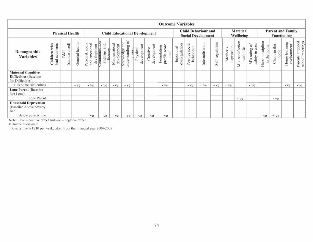
Outcome Variables

Physical Health Child Educational Development Child Behaviour and Social Development

Maternal Wellbeing

Parent and Family Functioning

Demographic Variables

Chi

ldre

n w

ho

had

acci

dent

s

BM

I(s

tand

ardi

sed)

Gen

eral

hea

lth

Pers

onal

, soc

ial

and

emot

iona

lde

velo

pmen

tC

omm

unic

atio

nla

ngua

ge a

nd

liter

acy

Mat

hem

atic

alde

velo

pmen

tK

now

ledg

e an

dun

ders

tand

ing

ofth

e w

orld

Phys

ical

deve

lopm

ent

Cre

ativ

ede

velo

pmen

t

Foun

datio

npr

ofile

scor

eto

tal

Emot

iona

ldy

sreg

ulat

ion

Posi

tive

soci

albe

havi

our

Inte

rnal

isat

ion

Self

regu

latio

n

Mot

her’

s de

pres

sion

M’s

sat

isfa

ctio

n w

ith li

fe

M’s

ratin

g of

sa

fety

in a

rea

Har

sh d

isci

plin

ein

the

hom

e

Cha

os in

the

hom

e

Hom

e le

arni

ngen

viro

nmen

t

Pare

nts a

ttend

edsc

hool

mee

tings

Maternal Cognitive Difficulties (Baseline No Difficulties)

Has Some Difficulties - ve - ve - ve - ve - ve - ve - ve + ve - ve + ve - ve - ve -ve Lone Parent (Baseline Not Lone)

Lone Parent - ve - ve Household Deprivation (Baseline Above poverty line+)

Below poverty line - ve - ve - ve - ve - ve - ve - ve - ve + ve

Note: +ve = positive effect and –ve = negative effect # Unable to estimate

+Poverty line is £210 per week, taken from the financial year 2004-2005

74

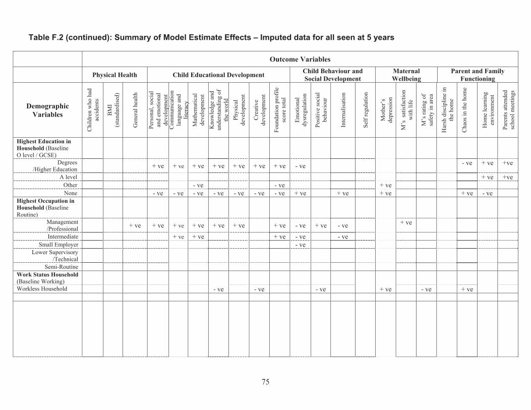
Table F.2 (continued): Summary of Model Estimate Effects – Imputed data for all seen at 5 years

Outcome Variables

Physical Health Child Educational Development Child Behaviour and Social Development

Maternal Wellbeing

Parent and Family Functioning

Demographic Variables

Chi

ldre

n w

ho h

ad

acci

dent

s

BM

I(s

tand

ardi

sed)

Gen

eral

hea

lth

Pers

onal

, soc

ial

and

emot

iona

l de

velo

pmen

tC

omm

unic

atio

nla

ngua

ge a

nd

liter

acy

Mat

hem

atic

alde

velo

pmen

t K

now

ledg

e an

dun

ders

tand

ing

ofth

e w

orld

Phys

ical

deve

lopm

ent

Cre

ativ

e de

velo

pmen

t

Foun

datio

n pr

ofile

sc

ore

tota

l

Emot

iona

ldy

sreg

ulat

ion

Posi

tive

soci

albe

havi

our

Inte

rnal

isat

ion

Self

regu

latio

n

Mot

her’

sde

pres

sion

M’s

sat

isfa

ctio

nw

ith li

fe

M’s

ratin

g of

safe

ty in

are

a

Har

sh d

isci

plin

e in

th

e ho

me

Cha

os in

the

hom

e

Hom

e le

arni

ngen

viro

nmen

t

Pare

nts a

ttend

edsc

hool

mee

tings

Highest Education in Household (Baseline O level / GCSE)

Degrees /Higher Education

A level Other None

+ ve

- ve

+ ve

- ve

+ ve

- ve - ve

+ ve

- ve

+ ve

- ve

+ ve

- ve

+ ve

- ve - ve

- ve

+ ve + ve + ve + ve

- ve

+ ve

+ ve

+ ve

- ve

+ve

+v

Highest Occupation in Household (Baseline Routine)

Management /Professional Intermediate

Small Employer Lower Supervisory

/Technical Semi-Routine

+ ve + ve + ve

+ ve

+ ve

+ ve

+ ve + ve + ve

+ ve

- ve

- ve - ve

+ ve - ve

- ve

+ ve

Work Status Household (Baseline Working) Workless Household - ve - ve - ve + ve - ve + ve

e

75

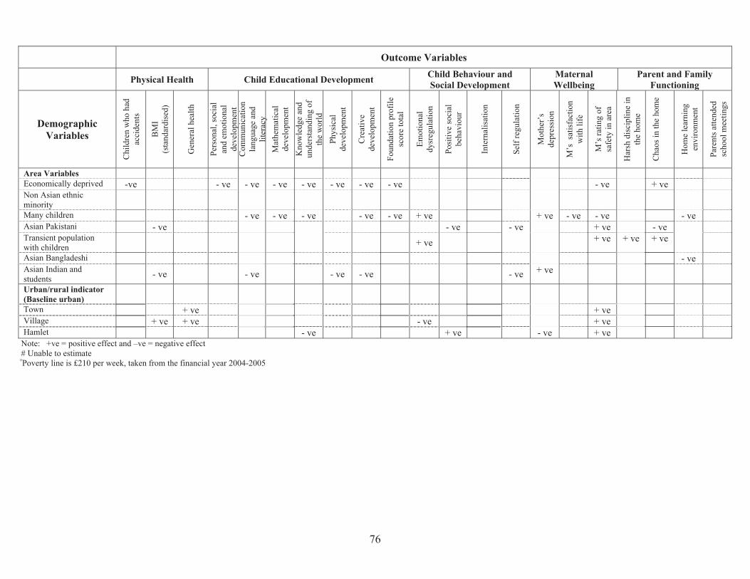
Outcome Variables

Physical Health Child Educational Development Child Behaviour and Social Development

Maternal Wellbeing

Parent and Family Functioning

Demographic who

had

dent

s

MI rdis

ed)

heal

th

Pers

onal

, sci

al

oan

d em

al

otio

nde

velo

pmen

t

nica

tion

g a

nla

ngua

ed

lite

acy

m

athe

atic

alde

velo

men

t p

K

now

ledg

e an

d

unde

rsta

ndin

g of

the

dw

orl

sica

lde

velo

men

t p

Cre

ive

atde

velo

men

t p

Foun

datio

n pr

ile

ofsc

ore

tal

to tion

Em

oal

ulat

ion

Posi

tive

sia

l oc

viou

r

Inte

rna

ion

lisat

Self

rela

tion

gu her’

sss

ion

isfa

ctio

nw

ith

fe

li ting

ofin

are

a

Har

sh d

isin

ci

plin

e th

e h

me

o the

hom

e H

ome

lear

ning

nmen

t

atte

nd

Pare

nts

edm

eetin

gs

Variables C

hild

ren i

acc B

(sta

nda

Gen

eral

Com

mu r

M

Phy

dysr

eg

beha

Mot

depr

e

M’s

sat

M’s

rasa

fety

Cha

os in

envi

ro

scho

ol

Area Variables Economically deprived -ve - ve - ve - ve - ve - ve - ve - ve - ve + ve Non Asian ethnic

minority Many children - ve - ve - ve - ve - ve + ve + ve - ve - ve - ve Asian Pakistani - ve - ve - ve + ve - ve Transient population with children + ve + ve + ve + ve

Asian Bangladeshi - ve Asian Indian and students - ve - ve - ve - ve - ve + ve

Urban/rural indicator (Baseline urban) Town + ve + ve Village + ve + ve - ve + ve Hamlet - ve + ve - ve + ve

Note: +ve = positive effect and –ve = negative effect # Unable to estimate +Poverty line is £210 per week, taken from the financial year 2004-2005

76

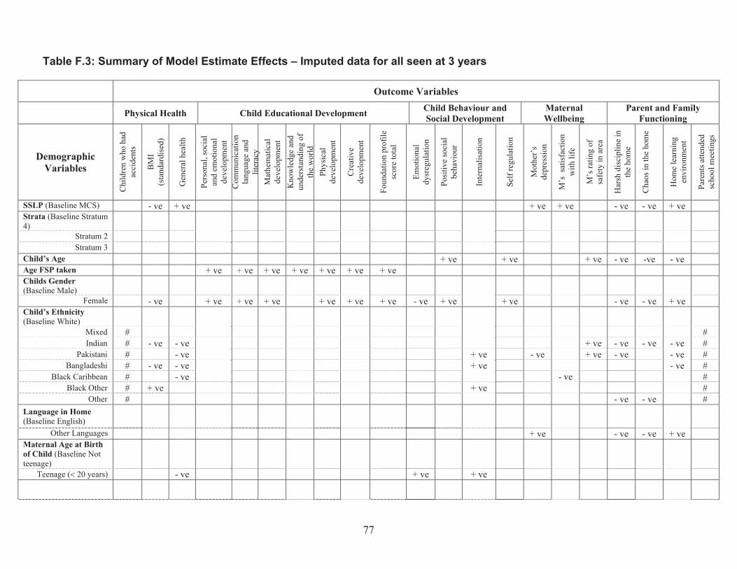
Table F.3: Summary of Model Estimate Effects – Imputed data for all seen at 3 years

Outcome Variables

Physical Health Child Educational Development Child Behaviour and Social Development

Maternal Wellbeing

Parent and Family Functioning

Demographic Variables

Chi

ldre

n w

ho h

ad

acci

dent

s

BM

I(s

tand

ardi

sed)

Gen

eral

hea

lth

Pers

onal

, soc

ial

and

emot

iona

l de

velo

pmen

t C

omm

unic

atio

nla

ngua

ge a

nd

liter

acy

Mat

hem

atic

alde

velo

pmen

t K

now

ledg

e an

dun

ders

tand

ing

ofth

e w

orld

Phys

ical

deve

lopm

ent

Cre

ativ

e de

velo

pmen

t

Foun

datio

n pr

ofile

sc

ore

tota

l

Emot

iona

ldy

sreg

ulat

ion

Posi

tive

soci

albe

havi

our

Inte

rnal

isat

ion

Self

regu

latio

n

Mot

her’

sde

pres

sion

M’s

sat

isfa

ctio

nw

ith li

fe

M’s

ratin

g of

safe

ty in

are

a

Har

sh d

isci

plin

e in

th

e ho

me

Cha

os in

the

hom

e

Hom

e le

arni

ngen

viro

nmen

t

Pare

nts a

ttend

edsc

hool

mee

tings

SSLP (Baseline MCS) - ve + ve + ve + ve - ve - ve + ve Strata (Baseline Stratum 4)

Stratum 2 Stratum 3

Child’s Age + ve + ve + ve - ve -ve - ve Age FSP taken + ve + ve + ve + ve + ve + ve + ve Childs Gender (Baseline Male)

Female - ve + ve + ve + ve + ve + ve + ve - ve + ve + ve - ve - ve + ve Child’s Ethnicity (Baseline White)

Mixed Indian

Pakistani Bangladeshi

Black Caribbean Black Other

Other

# # # # # # #

- ve

- ve

+ ve

- ve - ve - ve - ve

+ ve + ve

+ ve

- ve

- ve

+ ve + ve

- ve - ve

- ve

- ve

- ve

- ve - ve - ve

# # # # # # #

Language in Home (Baseline English)

Other Languages + ve - ve - ve + ve Maternal Age at Birth of Child (Baseline Not teenage)

Teenage (� 20 years) - ve + ve + ve

77

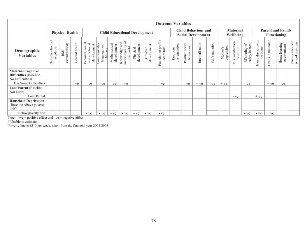
Outcome Variables

Physical Health Child Educational Development Child Behaviour and Social Development

Maternal Wellbeing

Parent and Family Functioning

Demographic Variables

Chi

ldre

n w

ho h

ad

acci

dent

s

BM

I(s

tand

ardi

sed)

Gen

eral

hea

lth

Pers

onal

, soc

ial

and

emot

iona

l de

velo

pmen

t C

omm

unic

atio

nla

ngua

ge a

nd

liter

acy

Mat

hem

atic

alde

velo

pmen

t K

now

ledg

e an

dun

ders

tand

ing

ofth

e w

orld

Phys

ical

deve

lopm

ent

Cre

ativ

e de

velo

pmen

t

Foun

datio

n pr

ofile

sc

ore

tota

l

Emot

iona

ldy

sreg

ulat

ion

Posi

tive

soci

al

beha

viou

r

Inte

rnal

isat

ion

Self

regu

latio

n

Mot

her’

sde

pres

sion

M’s

sat

isfa

ctio

nw

ith li

fe

M’s

ratin

g of

safe

ty in

are

a

Har

sh d

isci

plin

e in

th

e ho

me

Cha

os in

the

hom

e

Hom

e le

arni

ngen

viro

nmen

t

Pare

nts a

ttend

edsc

hool

mee

tings

Maternal Cognitive Difficulties (Baseline No Difficulties)

Has Some Difficulties - ve - ve - ve - ve - ve - ve - ve + ve - ve + ve - ve + ve - ve Lone Parent (Baseline Not Lone)

Lone Parent - ve + ve Household Deprivation (Baseline Above poverty line+)

Below poverty line - ve - ve - ve - ve - ve - ve - ve - ve - ve + ve

Note: +ve = positive effect and –ve = negative effect # Unable to estimate

+Poverty line is £210 per week, taken from the financial year 2004-2005

78

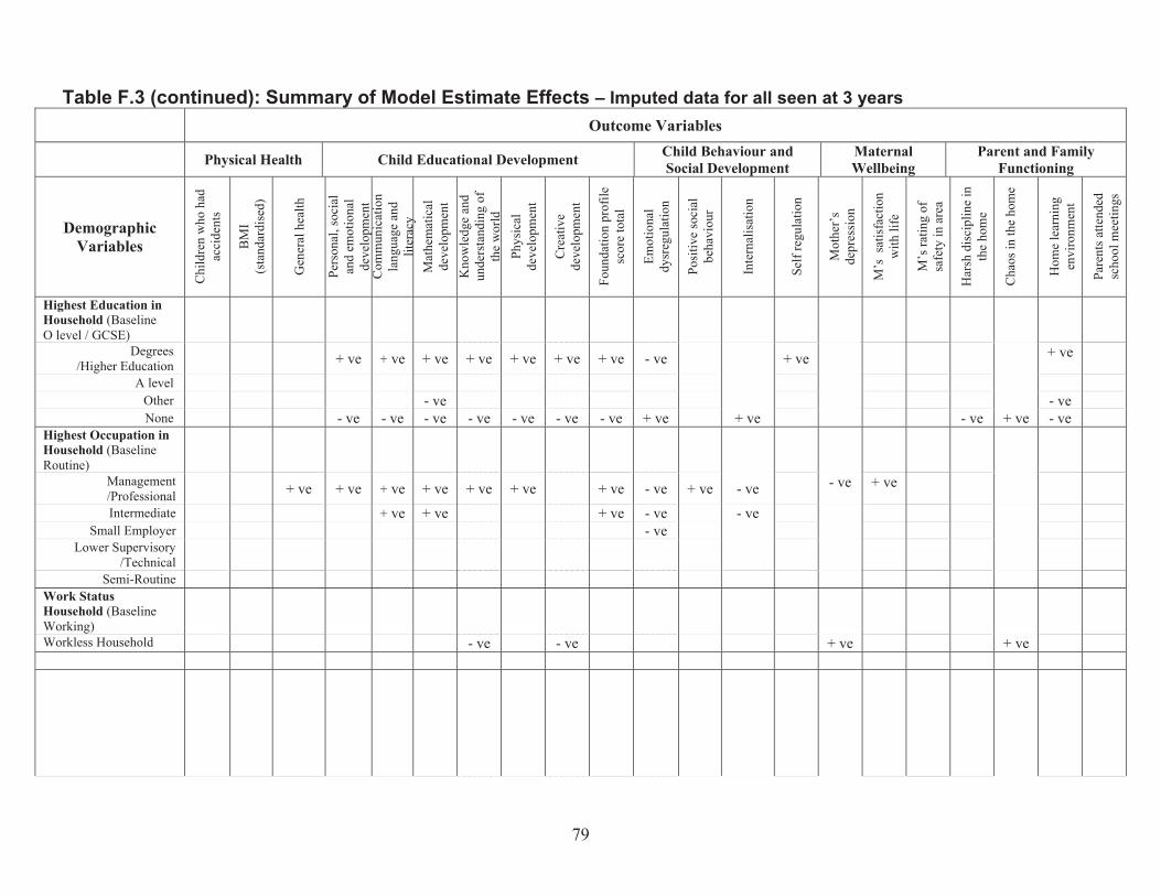
Outcome Variables

Physical Health Child Educational Development Child Behaviour and Social Development

Maternal Wellbeing

Parent and Family Functioning

Demographic Variables

Chi

ldre

n w

ho h

ad

acci

dent

s

BM

I(s

tand

ardi

sed)

Gen

eral

hea

lth

Pers

onal

, soc

ial

and

emot

iona

l de

velo

pmen

tC

omm

unic

atio

nla

ngua

ge a

nd

liter

acy

Mat

hem

atic

alde

velo

pmen

t K

now

ledg

e an

dun

ders

tand

ing

ofth

e w

orld

Phys

ical

deve

lopm

ent

Cre

ativ

e de

velo

pmen

t

Foun

datio

n pr

ofile

sc

ore

tota

l

Emot

iona

ldy

sreg

ulat

ion

Posi

tive

soci

albe

havi

our

Inte

rnal

isat

ion

Self

regu

latio

n

Mot

her’

sde

pres

sion

M’s

sat

isfa

ctio

nw

ith li

fe

M’s

ratin

g of

safe

ty in

are

a

Har

sh d

isci

plin

e in

th

e ho

me

Cha

os in

the

hom

e

Hom

e le

arni

ngen

viro

nmen

t

Pare

nts a

ttend

edsc

hool

mee

tings

Highest Education in Household (Baseline O level / GCSE)

Degrees /Higher Education

A level Other None

+ ve

- ve

+ ve

- ve

+ ve

- ve - ve

+ ve

- ve

+ ve

- ve

+ ve

- ve

+ ve

- ve

- ve

+ ve + ve

+ ve

- ve + ve

+ ve

- ve - ve

Highest Occupation in Household (Baseline Routine)

Management /Professional Intermediate

Small Employer Lower Supervisory

/Technical Semi-Routine

+ ve + ve + ve

+ ve

+ ve

+ ve

+ ve + ve + ve

+ ve

- ve

- ve - ve

+ ve - ve

- ve

- ve + ve

Work Status Household (Baseline Working) Workless Household - ve - ve + ve + ve

Table F.3 (continued): Summary of Model Estimate Effects – Imputed data for all seen at 3 years

79

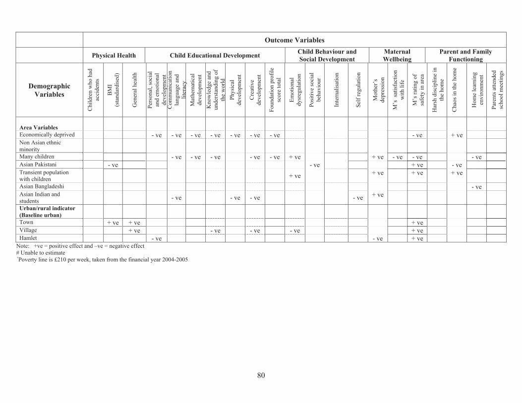
Outcome Variables

Physical Health Child Educational Development Child Behaviour and Social Development

Maternal Wellbeing

Parent and Family Functioning

Demographic Variables

Chi

ldre

n w

ho h

ad

acci

dent

s

BM

I(s

tand

ardi

sed)

Gen

eral

hea

lth

Pers

onal

, soc

ial

and

emot

iona

l de

velo

pmen

tC

omm

unic

atio

nla

ngua

ge a

nd

liter

acy

Mat

hem

atic

alde

velo

pmen

t K

now

ledg

e an

dun

ders

tand

ing

ofth

e w

orld

Phys

ical

deve

lopm

ent

Cre

ativ

e de

velo

pmen

t

Foun

datio

n pr

ofile

sc

ore

tota

l

Emot

iona

ldy

sreg

ulat

ion

Posi

tive

soci

al

beha

viou

r

Inte

rnal

isat

ion

Self

regu

latio

n

Mot

her’

sde

pres

sion

M’s

sat

isfa

ctio

nw

ith li

fe

M’s

ratin

g of

safe

ty in

are

a

Har

sh d

isci

plin

e in

th

e ho

me

Cha

os in

the

hom

e

Hom

e le

arni

ngen

viro

nmen

t

Pare

nts a

ttend

edsc

hool

mee

tings

Area Variables Economically deprived - ve - ve - ve - ve - ve - ve - ve - ve + ve Non Asian ethnic minority Many children - ve - ve - ve - ve - ve + ve + ve - ve - ve - ve Asian Pakistani - ve - ve + ve - ve Transient population with children + ve + ve + ve + ve

Asian Bangladeshi - ve Asian Indian and students - ve - ve - ve - ve + ve

Urban/rural indicator (Baseline urban) Town Village Hamlet

+ ve + ve + ve

- ve - ve - ve - ve

- ve

+ ve + ve + ve

Note: +ve = positive effect and –ve = negative effect # Unable to estimate

+Poverty line is £210 per week, taken from the financial year 2004-2005

80

Appendix G: SSLP vs. MCS by demographic group interactions Note that estimated values are derived from models using interactions of interest (baseline characteristics assumed for all other variables).

In section 3.3 the results of analyses that considered whether there were differences in SSLP effects for different demographic subgroups were discussed. In Appendix G tables are presented that show whether there was a significant interaction between SSLP/MCS status and subgroup status. Where the p-value is less than .05 then this indicates a statistically significant interaction between SSLP/MCS status and subgroup status.

The results are presented firstly for analyses of the complete cases (G1), secondly for imputed data for all seen at 5 years (G2), and thirdly for imputed data for all seen at 3 years (G3).

81

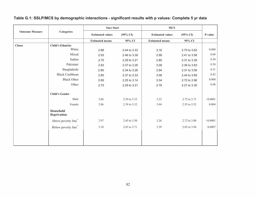
Table G.1: SSLP/MCS by demographic interactions - significant results with p values: Complete 5 yr data

Outcome Measure Categories Sure Start MCS

P-valueEstimated values (95% CI) Estimated values (95% CI)

Estimated means 95% CI Estimated means 95% CI Chaos Child’s Ethnicity

White 2.88 2.44 to 3.33 3.16 2.70 to 3.62 0.000

Mixed 2.93 2.46 to 3.39 2.99 2.41 to 3.56 0.68

Indian 2.75 2.29 to 3.21 2.85 2.31 to 3.39 0.50

Pakistani 2.83 2.37 to 3.29 3.09 2.36 to 3.83 0.38

Bangladeshi 2.80 2.34 to 3.26 2.94 2.31 to 3.56 0.51

Black Caribbean 2.85 2.37 to 3.33 3.06 2.44 to 3.69 0.42

Black Other 2.69 2.25 to 3.14 3.34 2.72 to 3.96 0.000

Other

Child’s Gender

2.75 2.29 to 3.21 2.76 2.21 to 3.30 0.98

Male 2.86 2.39 to 3.33 3.22 2.72 to 3.71 <0.0001

Female

Household Deprivation

2.86 2.39 to 3.32 3.04 2.55 to 3.52 0.004

Above poverty line+ 2.97 2.45 to 3.50 3.26 2.72 to 3.80 <0.0001

Below poverty line+ 3.18 2.65 to 3.71 3.39 2.85 to 3.94 0.0007

82

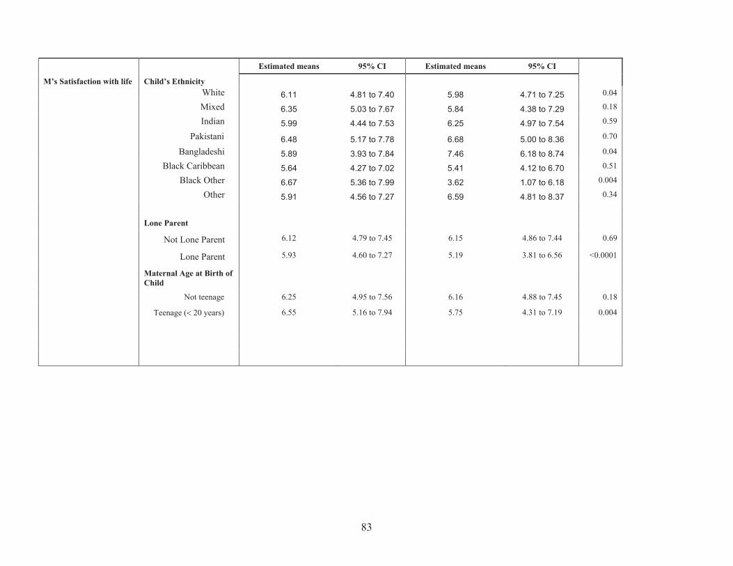
M’s Satisfaction with life Child’s Ethnicity

Estimated means 95% CI Estimated means 95% CI

White 6.11 4.81 to 7.40 5.98 4.71 to 7.25 0.04

Mixed 6.35 5.03 to 7.67 5.84 4.38 to 7.29 0.18

Indian 5.99 4.44 to 7.53 6.25 4.97 to 7.54 0.59

Pakistani 6.48 5.17 to 7.78 6.68 5.00 to 8.36 0.70

Bangladeshi 5.89 3.93 to 7.84 7.46 6.18 to 8.74 0.04

Black Caribbean 5.64 4.27 to 7.02 5.41 4.12 to 6.70 0.51

Black Other 6.67 5.36 to 7.99 3.62 1.07 to 6.18 0.004

Other

Lone Parent

5.91 4.56 to 7.27 6.59 4.81 to 8.37 0.34

Not Lone Parent 6.12 4.79 to 7.45 6.15 4.86 to 7.44 0.69

Lone Parent

Maternal Age at Birth of Child

5.93 4.60 to 7.27 5.19 3.81 to 6.56 <0.0001

Not teenage 6.25 4.95 to 7.56 6.16 4.88 to 7.45 0.18

Teenage (� 20 years) 6.55 5.16 to 7.94 5.75 4.31 to 7.19 0.004

83

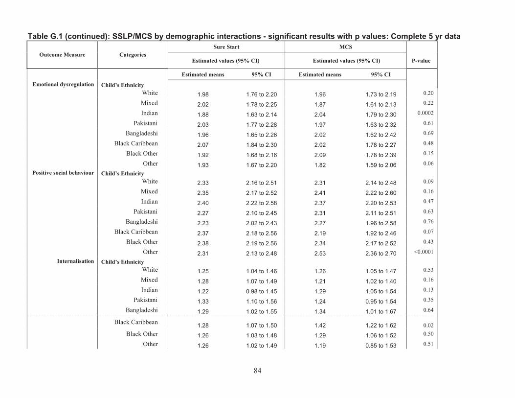
Table G.1 (continued): SSLP/MCS by demographic interactions - significant results with p values: Complete 5 yr data

Outcome Measure Categories Sure Start MCS

P-valueEstimated values (95% CI) Estimated values (95% CI)

Estimated means 95% CI Estimated means 95% CI

Emotional dysregulation Child’s Ethnicity White 1.98 1.76 to 2.20 1.96 1.73 to 2.19 0.20

Mixed 2.02 1.78 to 2.25 1.87 1.61 to 2.13 0.22

Indian 1.88 1.63 to 2.14 2.04 1.79 to 2.30 0.0002

Pakistani 2.03 1.77 to 2.28 1.97 1.63 to 2.32 0.61

Bangladeshi 1.96 1.65 to 2.26 2.02 1.62 to 2.42 0.69

Black Caribbean 2.07 1.84 to 2.30 2.02 1.78 to 2.27 0.48

Black Other 1.92 1.68 to 2.16 2.09 1.78 to 2.39 0.15

Positive social behaviour Other

Child’s Ethnicity 1.93 1.67 to 2.20 1.82 1.59 to 2.06 0.06

White 2.33 2.16 to 2.51 2.31 2.14 to 2.48 0.09

Mixed 2.35 2.17 to 2.52 2.41 2.22 to 2.60 0.16

Indian 2.40 2.22 to 2.58 2.37 2.20 to 2.53 0.47

Pakistani 2.27 2.10 to 2.45 2.31 2.11 to 2.51 0.63

Bangladeshi 2.23 2.02 to 2.43 2.27 1.96 to 2.58 0.76

Black Caribbean 2.37 2.18 to 2.56 2.19 1.92 to 2.46 0.07

Black Other 2.38 2.19 to 2.56 2.34 2.17 to 2.52 0.43

Internalisation Other

Child’s Ethnicity 2.31 2.13 to 2.48 2.53 2.36 to 2.70 <0.0001

White 1.25 1.04 to 1.46 1.26 1.05 to 1.47 0.53

Mixed 1.28 1.07 to 1.49 1.21 1.02 to 1.40 0.16

Indian 1.22 0.98 to 1.45 1.29 1.05 to 1.54 0.13

Pakistani 1.33 1.10 to 1.56 1.24 0.95 to 1.54 0.35

Bangladeshi 1.29 1.02 to 1.55 1.34 1.01 to 1.67 0.64

Black Caribbean 1.28 1.07 to 1.50 1.42 1.22 to 1.62 0.02 Black Other 1.26 1.03 to 1.48 1.29 1.06 to 1.52 0.50

Other 1.26 1.02 to 1.49 1.19 0.85 to 1.53 0.51

84

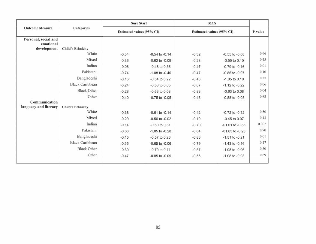
Outcome Measure Categories Sure Start MCS

P-valueEstimated values (95% CI) Estimated values (95% CI)

Personal, social and emotional

development Child’s Ethnicity White -0.34 -0.54 to -0.14 -0.32 -0.55 to -0.08 0.66

Mixed -0.36 -0.62 to -0.09 -0.23 -0.55 to 0.10 0.45

Indian -0.06 -0.48 to 0.35 -0.47 -0.79 to -0.16 0.01

Pakistani -0.74 -1.08 to -0.40 -0.47 -0.86 to -0.07 0.10

Bangladeshi -0.16 -0.54 to 0.22 -0.48 -1.05 to 0.10 0.27

Black Caribbean -0.24 -0.53 to 0.05 -0.67 -1.12 to -0.22 0.06

Black Other -0.28 -0.63 to 0.08 -0.83 -0.63 to 0.08 0.04

Communication language and literacy

Other

Child’s Ethnicity

-0.40 -0.75 to -0.05 -0.48 -0.88 to -0.08 0.62

White -0.38 -0.61 to -0.14 -0.42 -0.72 to -0.12 0.50

Mixed -0.29 -0.56 to -0.02 -0.19 -0.45 to 0.07 0.43

Indian -0.14 -0.60 to 0.31 -0.70 -01.01 to -0.38 0.002

Pakistani -0.66 -1.05 to -0.28 -0.64 -01.05 to -0.23 0.90

Bangladeshi -0.15 -0.57 to 0.26 -0.86 -1.51 to -0.21 0.01

Black Caribbean -0.35 -0.65 to -0.06 -0.79 -1.43 to -0.16 0.17

Black Other -0.30 -0.70 to 0.11 -0.57 -1.08 to -0.06 0.30

Other -0.47 -0.85 to -0.09 -0.56 -1.08 to -0.03 0.69

85

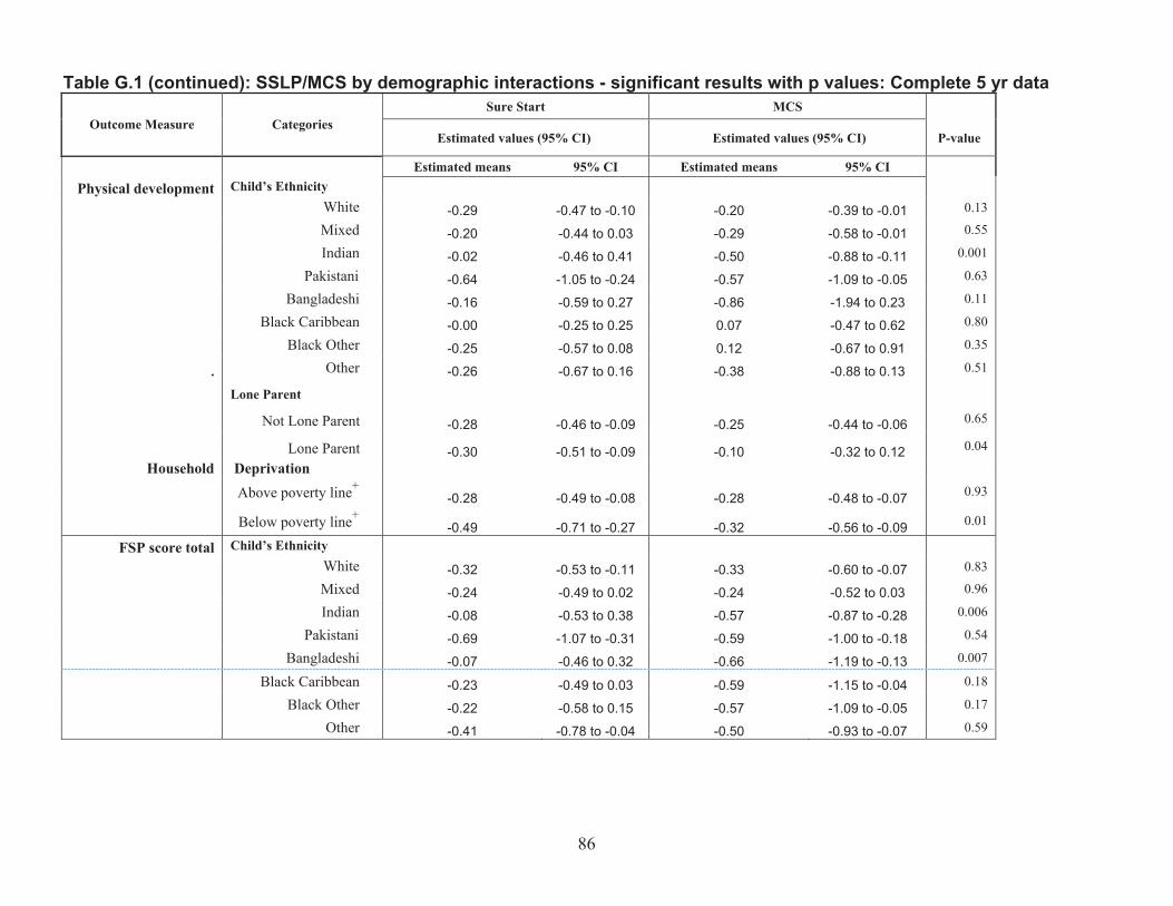
Table G.1 (continued): SSLP/MCS by demographic interactions - significant results with p values: Complete 5 yr data

Outcome Measure Categories Sure Start MCS

P-valueEstimated values (95% CI) Estimated values (95% CI)

Estimated means 95% CI Estimated means 95% CI

Physical development Child’s Ethnicity White -0.29 -0.47 to -0.10 -0.20 -0.39 to -0.01 0.13

Mixed -0.20 -0.44 to 0.03 -0.29 -0.58 to -0.01 0.55

Indian -0.02 -0.46 to 0.41 -0.50 -0.88 to -0.11 0.001

Pakistani -0.64 -1.05 to -0.24 -0.57 -1.09 to -0.05 0.63

Bangladeshi -0.16 -0.59 to 0.27 -0.86 -1.94 to 0.23 0.11

Black Caribbean -0.00 -0.25 to 0.25 0.07 -0.47 to 0.62 0.80

Black Other -0.25 -0.57 to 0.08 0.12 -0.67 to 0.91 0.35

. Other

Lone Parent

-0.26 -0.67 to 0.16 -0.38 -0.88 to 0.13 0.51

Not Lone Parent -0.28 -0.46 to -0.09 -0.25 -0.44 to -0.06 0.65

Household Lone Parent

Deprivation -0.30 -0.51 to -0.09 -0.10 -0.32 to 0.12 0.04

Above poverty line+ -0.28 -0.49 to -0.08 -0.28 -0.48 to -0.07 0.93

Below poverty line+ -0.49 -0.71 to -0.27 -0.32 -0.56 to -0.09 0.01

FSP score total Child’s Ethnicity White -0.32 -0.53 to -0.11 -0.33 -0.60 to -0.07 0.83

Mixed -0.24 -0.49 to 0.02 -0.24 -0.52 to 0.03 0.96

Indian -0.08 -0.53 to 0.38 -0.57 -0.87 to -0.28 0.006

Pakistani -0.69 -1.07 to -0.31 -0.59 -1.00 to -0.18 0.54

Bangladeshi -0.07 -0.46 to 0.32 -0.66 -1.19 to -0.13 0.007

Black Caribbean -0.23 -0.49 to 0.03 -0.59 -1.15 to -0.04 0.18

Black Other -0.22 -0.58 to 0.15 -0.57 -1.09 to -0.05 0.17

Other -0.41 -0.78 to -0.04 -0.50 -0.93 to -0.07 0.59

86

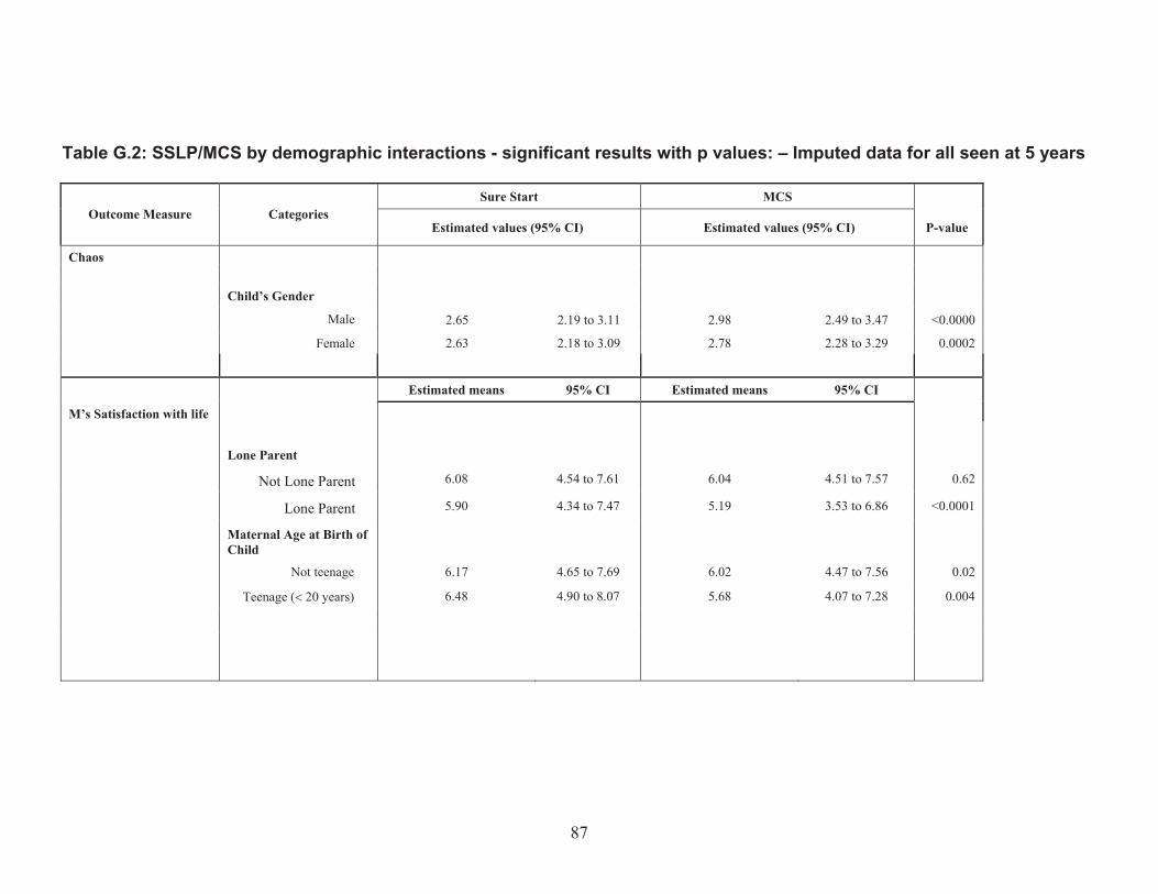
Table G.2: SSLP/MCS by demographic interactions - significant results with p values: – Imputed data for all seen at 5 years

Outcome Measure Categories Sure Start MCS

P-valueEstimated values (95% CI) Estimated values (95% CI)

Chaos

Child’s Gender

Male

Female

2.65 2.19 to 3.11

2.63 2.18 to 3.09

2.98 2.49 to 3.47

2.78 2.28 to 3.29

<0.0000

0.0002

Estimated means 95% CI Estimated means 95% CI

0.62

<0.0001

0.02

0.004

M’s Satisfaction with life

Lone Parent

Not Lone Parent

Lone Parent

Maternal Age at Birth of Child

Not teenage

Teenage (� 20 years)

6.08 4.54 to 7.61

5.90 4.34 to 7.47

6.17 4.65 to 7.69

6.48 4.90 to 8.07

6.04 4.51 to 7.57

5.19 3.53 to 6.86

6.02 4.47 to 7.56

5.68 4.07 to 7.28

87

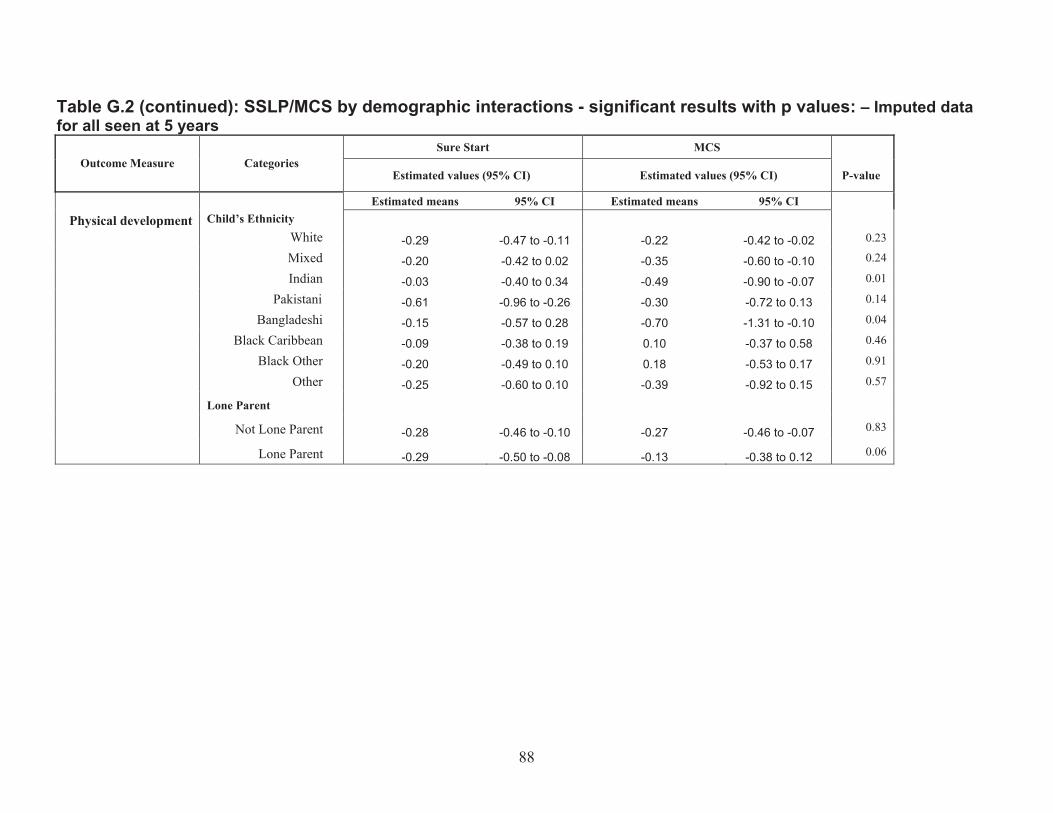
Table G.2 (continued): SSLP/MCS by demographic interactions - significant results with p values: – Imputed data for all seen at 5 years�

Outcome Measure Categories Sure Start MCS

P-valueEstimated values (95% CI) Estimated values (95% CI)

Estimated means 95% CI Estimated means 95% CI Physical development Child’s Ethnicity

White -0.29 -0.47 to -0.11 -0.22 -0.42 to -0.02 0.23

Mixed -0.20 -0.42 to 0.02 -0.35 -0.60 to -0.10 0.24

Indian -0.03 -0.40 to 0.34 -0.49 -0.90 to -0.07 0.01

Pakistani -0.61 -0.96 to -0.26 -0.30 -0.72 to 0.13 0.14

Bangladeshi -0.15 -0.57 to 0.28 -0.70 -1.31 to -0.10 0.04

Black Caribbean -0.09 -0.38 to 0.19 0.10 -0.37 to 0.58 0.46

Black Other -0.20 -0.49 to 0.10 0.18 -0.53 to 0.17 0.91

Other

Lone Parent

-0.25 -0.60 to 0.10 -0.39 -0.92 to 0.15 0.57

Not Lone Parent -0.28 -0.46 to -0.10 -0.27 -0.46 to -0.07 0.83

Lone Parent -0.29 -0.50 to -0.08 -0.13 -0.38 to 0.12 0.06

88

�

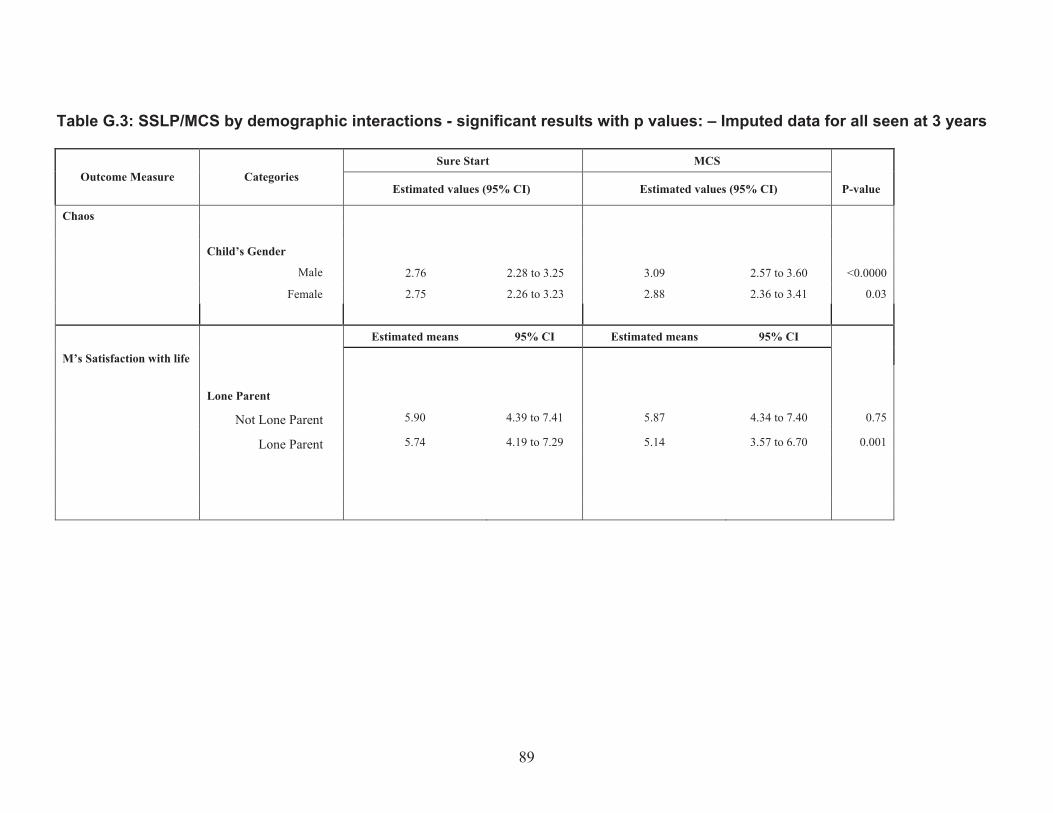
Table G.3: SSLP/MCS by demographic interactions - significant results with p values: – Imputed data for all seen at 3 years

Outcome Measure Categories Sure Start MCS

P-valueEstimated values (95% CI) Estimated values (95% CI)

Chaos

Child’s Gender

Male

Female

2.76 2.28 to 3.25

2.75 2.26 to 3.23

3.09 2.57 to 3.60

2.88 2.36 to 3.41

<0.0000

0.03

Estimated means 95% CI Estimated means 95% CI

0.75

0.001

M’s Satisfaction with life

Lone Parent

Not Lone Parent

Lone Parent

5.90 4.39 to 7.41

5.74 4.19 to 7.29

5.87 4.34 to 7.40

5.14 3.57 to 6.70

89

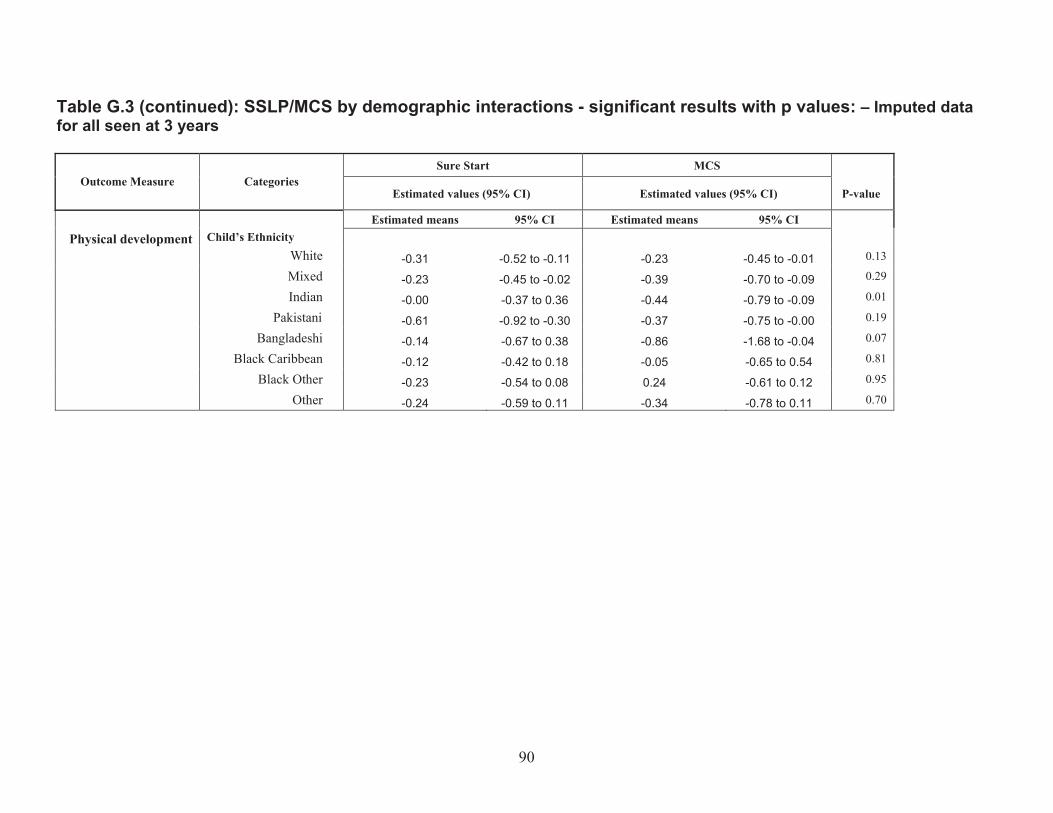
Table G.3 (continued): SSLP/MCS by demographic interactions - significant results with p values: – Imputed data for all seen at 3 years

Outcome Measure Categories Sure Start MCS

P-valueEstimated values (95% CI) Estimated values (95% CI)

Estimated means 95% CI Estimated means 95% CI

0.13

0.29

0.01

0.19

0.07

0.81

0.95

0.70

Physical development Child’s Ethnicity White Mixed Indian

Pakistani Bangladeshi

Black Caribbean Black Other

Other

-0.31 -0.52 to -0.11

-0.23 -0.45 to -0.02

-0.00 -0.37 to 0.36

-0.61 -0.92 to -0.30

-0.14 -0.67 to 0.38

-0.12 -0.42 to 0.18

-0.23 -0.54 to 0.08

-0.24 -0.59 to 0.11

-0.23 -0.45 to -0.01

-0.39 -0.70 to -0.09

-0.44 -0.79 to -0.09

-0.37 -0.75 to -0.00

-0.86 -1.68 to -0.04

-0.05 -0.65 to 0.54

0.24 -0.61 to 0.12

-0.34 -0.78 to 0.11

90

Ref: DFE-RR067

ISBN: 978-1-84775-826-2

© Department for Education

November 2010