Embed Size (px)
Citation preview

DI
SC
US
SI
ON
P
AP
ER
S
ER
IE
S
Forschungsinstitut zur Zukunft der ArbeitInstitute for the Study of Labor
The Impact of Short- and Long-term Participation Tax Rates on Labor Supply
IZA DP No. 9151
June 2015
Charlotte BartelsNico Pestel

The Impact of Short- and Long-Term
Participation Tax Rates on Labor Supply
Charlotte Bartels Freie Universität Berlin
Nico Pestel
IZA and ZEW
Discussion Paper No. 9151 June 2015
IZA
P.O. Box 7240 53072 Bonn
Germany
Phone: +49-228-3894-0 Fax: +49-228-3894-180
E-mail: [email protected]
Any opinions expressed here are those of the author(s) and not those of IZA. Research published in this series may include views on policy, but the institute itself takes no institutional policy positions. The IZA research network is committed to the IZA Guiding Principles of Research Integrity. The Institute for the Study of Labor (IZA) in Bonn is a local and virtual international research center and a place of communication between science, politics and business. IZA is an independent nonprofit organization supported by Deutsche Post Foundation. The center is associated with the University of Bonn and offers a stimulating research environment through its international network, workshops and conferences, data service, project support, research visits and doctoral program. IZA engages in (i) original and internationally competitive research in all fields of labor economics, (ii) development of policy concepts, and (iii) dissemination of research results and concepts to the interested public. IZA Discussion Papers often represent preliminary work and are circulated to encourage discussion. Citation of such a paper should account for its provisional character. A revised version may be available directly from the author.

IZA Discussion Paper No. 9151 June 2015
ABSTRACT
The Impact of Short- and Long-Term Participation Tax Rates on Labor Supply*
Generous income support programs as provided by European welfare states have often been blamed to hamper employment. This paper investigates the importance of incentives inherent in the tax-benefit system for the individual decision to take up work. Using German microdata over the period 1993-2010 we find that recent reforms in Germany increased work incentives at the extensive margin measured by the Participation Tax Rate (PTR), particularly for low-income individuals. Work incentives are even higher if the time horizon is extended to more than one year, pointing at an overestimation of the disincentives by standard measures. Regression analysis reveals that a decrease in the PTR increases the likelihood of taking up work significantly. JEL Classification: H24, H31, J22, J65 Keywords: labor force participation, work incentives, welfare, unemployment insurance,
income taxation Corresponding author: Charlotte Bartels Freie Universität Berlin Boltzmannstr. 20 14195 Berlin Germany E-mail: [email protected]
* The paper benefited from the comments of the editor and one anonymous referee. We thank Timm Bönke, Giacomo Corneo, Sebastian Eichfelder, Frank Fossen, Peter Haan and Victor Steiner as well as participants of the SSCW 2012, Verein für Socialpolitik 2012, ECINEQ 2013, IIPF 2014, SEEK 2014 and 13th Finanzwissenschaftler Workshop 2014 for helpful comments and suggestions.

1 Introduction
In many European welfare states, major reforms have been undertaken in the last
three decades to tackle the enduringly high unemployment rates. Under the general
impression that generous benefits and high marginal taxes were to blame for low
incentives to take up work, out-of-work benefits have been reduced and income taxes
cut. These reform efforts are backed by a wide range of empirical studies on labor
supply elasticities showing that behavioral responses are higher at the extensive
margin than at the intensive margin, particularly for low-income individuals. Hence,
a tax-benefit design misshapen at the extensive margin may create high efficiency
costs.
In Germany, rising unemployment after reunification in 1990 ushered in a
period of labor market and tax reforms. Beginning in 1994, eligibility for unem-
ployment benefits was tightened and sanctioning mechanisms introduced to push
the unemployed into work. Personal income tax reforms between 1998 and 2005
substantially reduced marginal and average tax rates particularly relieving the rich
(Corneo, 2005). The most radical changes, the so-called Hartz reforms, were intro-
duced between 2003 and 2005 slashing out-of-work benefits for low-income individ-
uals and long-term unemployed. However, the latter effect becomes only evident,
when analysing work incentives over several years.
This paper estimates work incentives in Germany at the extensive margin by
computing Participation Tax Rates (PTR) – a work incentive measure derived from
optimal tax theory – and examines the extent to which the presumed increase of
work incentives contributed to raise the probability for the unemployed to take up
work. First, we extend the analysis of work incentives to more than one year. A
three-year period is chosen to lift the time horizon above a minimum of two years
but maximizing the sample size of the balanced panel at the same time. Thereby,
important aspects can be included in the analysis which individuals maximizing util-
ity over time might consider: A working individual can experience earnings growth
over time driven by on-the-job-training and tenure. In contrast, a non-working in-
dividual receives benefits from unemployment insurance or social assistance which
are determined by institutional rules. In Germany, benefits from unemployment
1

insurance decline with the duration of unemployment. Hence, income differences
between working and non-working individuals tend to widen when extending the
measurement period. Moreover, human capital depreciation during unemployment
reduces future earnings potential. Two scenarios are developed in order to include
human capital depreciation into the PTR measure.
PTRs are computed for all individuals in the labor force independent of their
labor market status and demographic subgroups such as gender, employment level
and household type. Women are more likely to work part-time, particularly in
marginal employment, and are, thus, less often eligible for unemployment benefits
than men which in turn may generate lower PTRs. These may also vary over
household types. The financial reward for job take-up is largely determined by the
effect of joint taxation and benefit withdrawal in the presence of a second earner
and/or other income sources than labor earnings.
The main findings are as follows: First, long-term PTRs are significantly lower
than short-term PTRs. Hence, standard measures overestimate the disincentives
created by the German tax-benefit system. Three-year PTRs vary between 50%
and 65% depending on the earnings level, whereas one-year PTRs are 70-80%. Sec-
ond, the Hartz reforms reduce PTRs, particularly for low-income women. Their
long-term PTR declines from around 40% to about 30%. Third, including human
capital depreciation decreases the PTR, but the difference to the baseline scenario
becomes negligible after the reforms. Fourth, a lower PTR significantly increase
the probability to take up work in a time period of major changes in the German
tax-benefit system towards higher work incentives.
The paper is organized as follows: A brief literature review is given in Section
2. Data and basic concepts regarding the measurement of short-term and long-
term PTRs are outlined in Section 3. Section 4 provides an extensive discussion of
our results for short-term and long-term PTRs in Germany 1993–2010 by earnings
decile, earner type, age and gender and identifies driving factors behind PTRs in
Germany. The estimation strategy and regression results are presented and discussed
in Section 5. Section 6 concludes.
2

2 Literature Review
The literature on labor supply and optimal taxation distinguishes labor supply re-
sponses at the extensive and at the intensive margin. After the seminal contribution
of Mirrlees (1971) on optimal taxation at the intensive margin, Diamond (1980) de-
veloped an optimal tax model with labor supply responses at the extensive margin.
Saez (2002) first incorporated both responses at the intensive and extensive mar-
gin. In optimal tax theory, work incentives inherent in the tax-benefit system are
captured by the Effective Marginal Tax Rate (EMTR) at intensive margin and the
Participation Tax Rate (PTR) at the extensive margin. Diamond (1980), Saez
(2002) and, more recently, Jacquet et al. (2013) find that the optimal PTR can be
negative for lower income levels. The empirical literature has shown that the behav-
ioral response at the extensive margin exceeds the response at the intensive margin.
In particular, low-educated men and single mothers/women reveal higher and mar-
ried women lower extensive margin elasticities (see Chetty et al., 2013; Meghir and
Phillips, 2010, for an overview).
Both the growing theoretical literature and the empirical results on the size
of the response at the extensive margin triggered a number of studies estimating
PTRs for various tax-benefit systems. Several studies have analyzed PTRs across
European countries applying tax-benefit rules of 1998 and for the UK over time.
Cross-country studies on PTRs in EU countries are Immervoll et al. (2007), Im-
mervoll et al. (2009) and O’Donoghue (2011). These studies rely on the simulation
model EUROMOD based on the tax-benefit rules prevailing in the year 1998. Coun-
try studies on PTRs are, e.g., Dockery et al. (2011) for Australia, Adam et al. (2006)
and Brewer et al. (2008) for UK as well as Pirttilla and Selin (2011) for Sweden.
However, all contributions are based on a time horizon of only one year.
Usually, empirical studies on work incentives examine their effect on either
aggregate unemployment, unemployment duration or labor market participation
within particular social insurance programs such as pensions or sickness pay. To
our knowledge, we are the first to study the effect of a work incentive measure
incorporating the entire tax-benefit system on the probability to take up work.
3

3 Method and Data
3.1 Data
The analysis is based on a subsample from the SOEP survey years 1994 to 2011 with
incomes from 1993 to 2010. The SOEP is a representative panel study containing
individual and household data in Germany from 1984 onwards and was expanded
to the New German Laender after German reunification in 1990. All household
members are interviewed individually once they reach the age of 16.1
The sample only includes individuals who are aged between 25 and 54 to avoid
distortions due to early or partial retirement. Individuals who are self-employed or
civil servants and, as a consequence, did not necessarily contribute to unemployment
insurance are dropped as are disabled individuals. Only individuals belonging to
households classifiable as single, single parent or couples with or without children
are included. Furthermore, employed individuals with earnings below 33% of the
marginal employment threshold are dropped. Households enter the sample twice, if
both adults meet the requirements outlined above.
Participation decisions are largely correlated with characteristics like gender,
marital status and number of other household members. Figure 1 displays the
share of individuals taking up work switching their labor market status from non-
employment U to employment E. Men’s probability of taking up work from one year
to the next fluctuates around 3% until 2005 and around 3.5% thereafter. Women
are more likely to take up work with the probability fluctuating around 4% which
reflects increasing female labor market participation in Germany during this period.
Household earner types reveal both different patterns for men and women and
change over time as depicted by Figure 2. Women are more likely to be the second
earner working part-time and, consequently, earning less than their mostly full-time
working husband. The share of male and female single households increases over
time, but the majority of the observed men and women still lives in families. The
share of female sole earners increases slightly whereas the share of their male coun-
terparts decreases. Women are more likely to be a working single parent, whereas
1See Wagner et al. (2007) for further information on the SOEP.
4

Figure 1
.02
.03
.04
.05
1995 2000 2005 2010 1995 2000 2005 2010
Men Women
Pr(
UE
)
Source: SOEPv29 & IZAYMOD, own calculations.
Probability of taking up work (UE)
men are more likely to have a working partner.
5

Figure 2
0
20
40
60
80
10019
9319
9419
9519
9619
9719
9819
9920
0020
0120
0220
0320
0420
0520
0620
0720
0820
0920
10
1993
1994
1995
1996
1997
1998
1999
2000
2001
2002
2003
2004
2005
2006
2007
2008
2009
2010
Men Women
Single Sole earnerPrimary earner Secondary earner
%
Source: SOEPv29 & IZAYMOD, own calculations.
Composition of earner households
3.2 Measuring Participation Tax Rates
3.2.1 Standard Participation Tax Rates
As a context for our empirical analysis we assume that the individual i faces a binary
choice between the two labor market states E employed or U unemployed. The PTR
measures the change in household net taxes from labor market state E to U as a
fraction of individual earnings in labor market state E. Net taxes T paid by the
household h are income taxes th including social security contributions reduced by
benefits bh. Taxes and benefits are based on the household context for three reasons.
First, the loss of earned income in labor market state U may not only trigger off
eligibility rights for the unemployed individual but for other household members as
well. Second, joint taxation in Germany requires to consider a married couple as a
unit and to assess taxes on the basis of household income. Third, the impact of a
change in overall household income on taxes and benefits takes the extent of income
brought in by other household members and by other income sources into account.
An annual PTR can thus be denoted as
6

PTRih =T (yEh )− T (yUh )
yE,wi
, (1)
where yEh is gross household income, T (yEh ) is household net taxes and yE,wi is indi-
vidual labor earnings if the individual is in labor market state E. Gross household
income is the sum of labor earnings, asset income, private transfers, private pensions
and social security pensions of all household members. yUh is gross household income
and T (yUh ) is household net taxes if the individual is in labor market state U having
zero individual labor earnings.
If household net taxes are equal for both labor market states, then the PTR is
zero and incentives to take up work are not distorted. But a welfare state providing
income support in state U usually leads to tUh < bUh resulting in T (yUh ) < 0 as
unemployment benefits will surpass taxes paid for the declined household income
yUh . In sum, the change in net taxes will be positive in presence of a welfare state
and the PTR will be higher than zero for most individuals. The higher the PTR, the
more do generous income support programs reduce the financial gain from working.
The PTR is one, if the change in net taxes T (yEh )− T (yUh ) (numerator) is equal to
individual earnings yE,wi (denominator). In this case, there is no financial gain from
working. If out-of-work income support exceeds earnings, then the PTR can be even
greater than one.
In order to obtain a PTR for all individuals in the labor force independent
of their observed labor market status E or U , the non-observed state has to be
simulated. For the simulation, it is assumed that a change in one partner’s labor
supply behavior, i.e., giving up or taking up a job, does neither affect the labor
supply behavior of the other partner nor household income from other sources than
labor. This procedure is standard in the PTR literature (see, e.g., Immervoll et al.,
2007). We employ three simulation scenarios:
1. We take observed individual earnings yE,wi and gross household income yEh in
E from the SOEP data. Gross household income in U is then given by setting
individual earnings to zero and holding constant other household members’
labor income and household income from other sources, i.e., yUh = yEh − yE,wi .
7

However, this simulation scenario misses all those with zero earnings.
2. We simulate yE,wi for 20 hours of work for all individuals in the subsample
independently of their observed earnings and compute yEh and yUh accordingly.
Hourly wages are estimated by a standard Heckman procedure (Heckman,
1979).
3. We simulate yE,wi for 40 hours of work for all individuals in the subsample
independently of their observed earnings and compute yEh and yUh accordingly.
As for [2.], hourly wages are estimated by a standard Heckman procedure.
In a second step, we then apply the tax-benefit rules of the respective year to
obtain household taxes th and public transfers bh for both states E and U assuring
consistent assumptions regarding deductions etc. For example, household taxes paid
in state U are the sum of income tax tU,inch assessed on the basis of yUh , solidarity
surcharge tU,Sh and social security contributions sUj on spouse’s earnings yE,wj if the
spouse j is working in E. Household public transfers are the sum of unemployment
benefits, unemployment assistance, maternity benefits, social assistance, housing al-
lowances and child benefits. A potential increase in benefits when changing from
E to U will occur for unemployment benefits, unemployment assistance, social as-
sistance and housing allowances. In contrast, maternity benefits and child benefits
do not depend on household income and remain constant between E and U . All
simulations are based on IZAΨMOD, which is a microsimulation model for Germany
including a tax-benefit calculator for all years since the 1990s.2 Further details on
the regulations of the German tax-benefit-system are given in Appendix A.
3.2.2 Long-term Participation Tax Rates
The standard approach assesses work incentives over a one-year time horizon. But
economic theory on household economics predicts income pooling and budget smooth-
ing over long periods. Individuals may thus condition their participation decision
not only on next year’s expected income, but rather on a longer time horizon. A
working individual can achieve consecutive raises in earnings carving out a career.
2See Loffler et al. (2014) for a documentation of the simulation model.
8

In contrast, a transfer dependent individual receives a stable transfer income fixed
by the legislator, which only changes in the wake of reforms. Earnings-related un-
employment benefits are only paid during a limited period of time in Germany,
i.e., during one year for most individuals. This drop in benefits after exhaustion
of earnings-related unemployment benefits can only be accounted for by extending
the time horizon. Hence, while short-term PTRs are calculated for one year, long-
term PTRs are based on three years to shed light on work incentives in the longer
term. A three-year period is chosen to lift the time horizon above a minimum of two
years but maximizing the sample size of the balanced panel at the same time. To
calculate long-term PTRs a long-term income measure is needed. Long-term PTRs
of the observed simulation scenario are based on a balanced panel including only
individuals who were employed during all three years.
The long-term PTR is computed as the Net Present Value (NPV) of PTRs
over the respective period. Individual earnings ywitk and household net taxes T (yhtk)
in year k with base year t is discounted by dtk which is the inverse of the Consumer
Price Index (CPI) increase πtk from the base year t to year k. The PTR in the
long-term l is defined as
PTRliht =
NPV (T (yEh )− T (yUh ))
NPV (yE,wi )
(2)
=
∑Kk=1 dtk · [T (yEhk)− T (yUhk)]∑K
k=1 dtk · yE,wik
3.2.3 Participation Tax Rates with Human Capital Depreciation
Choosing labor market state U not only triggers potential transfers but also car-
ries costs such as matching costs to find a new employer, stigma, unemployment
scarring and reduced re-entry earnings as a result of human capital depreciation
(hcd). Not including the costs of non-participation would overestimate the disin-
centives, particularly if costs accumulate over time spent in non-participation. While
the loss in specific human capital is a once-for-all phenomenon due to the separa-
tion from the job, the loss in general human capital increases with the duration of
non-participation (Mincer and Ofek, 1982). Hence, the baseline scenario is slightly
9

modified to two alternative scenarios. In scenario 1, the individual now chooses be-
tween not working in the first year and working the two subsequent years (U ,E,E)
or not working at all (U ,U ,U). In scenario 2, the individual chooses between not
working for two years and working the year after (U ,U ,E) or not working at all
(U ,U ,U).
For the simulation of depreciated earnings at re-entry it is assumed that earn-
ings decline by α = 2% per year of non-participation.3 Depreciated earnings at
re-entry in k2 (scenario 1) or in k3 (scenario 2) are computed as a fraction of earn-
ings given in the data and are defined as
yEk,w,hcdi = yEk,w
i · (1− α)k−1 with k = 1, 2, 3 , (3)
where k indicates the number of periods being unemployed.
4 Results for Participation Tax Rates
Several factors lead to variation of PTRs among the population. Individual earnings
is a major determinant in the denominator of the PTR-formula. The PTR is higher,
the lower the wage and/or weekly working hours. On the other hand, real wage
growth may lead to lower PTRs and higher work incentives. Apart from earnings,
PTRs heavily depend on the household context that determines the change in net
household taxes between E and U in the numerator of the PTR-formula. High
PTRs can be generated by both high out-of-work income provided by the welfare
state and large reductions in household net taxes when changing to state U . Both
terms strongly depend on the level of spouse’s earnings and other household income
sources.
The PTR can be interpreted as the sum of the in-work tax rate and the out-
of-work gross replacement rate. A single median earner, whose only income source
is labor income, may serve as a stylized example to illustrate this interpretation.
3A number of studies estimates the earnings penalty or atrophy rate per year of non-participation. Results are mostly around or slightly higher than 1% (e.g. Kim and Polachek,1994), but some are even as high as 11% (Gregory and Jukes, 2001) earnings reduction per year.
10

A PTR of 80% for a single earning 24,000 Euro annually results from an in-work
tax rate equal to 11,00024,000
= 46% and an out-of-work gross benefit ratio equal to
8,20024,000
= 34%. Net taxes in E result from taxes on earnings of 11,000 Euros and
zero transfers. Net taxes in U result from zero taxes and unemployment benefits of
8,200 Euro. The net financial gain of taking up a job with a salary of 24,000 Euro
is 4,800 Euro (20% of 24,000). This may appear very small at the first sight. But
indeed, the German tax-benefit system creates high PTRs in European comparison.
Immervoll et al. (2007) find a median earner PTR slightly above 70% in Germany,
France, Sweden and Finland. Solely Denmark has higher PTRs. Median earner
PTRs in United Kingdom, Ireland, Austria and Italy are in the range of 50% to
60%. The German median earner faces comparably high taxes and social security
contributions combined with generous unemployment benefits. But as we will see
in the following, PTRs vary quite a lot over the working age population and over
time.
4.1 Short-term Participation Tax Rates by Earnings Decile
The development of short-term PTRs by earnings decile, gender and simulation
scenario over time is shown in Figure 3. Each graph presents median PTRs within
an earnings decile between 1993 and 2010. We first comment on PTRs based on
observed hours. Two features stand out.
First, PTRs increase with earnings. Men and women in the top decile face
a PTR of about 80%, whereas the PTR in the lowest decile is only about 60–70%
regardless of the simulation scenario. This occurs because of both lower benefits in
U and a lower tax wedge between E and U in the lowest decile. The number of
those eligible for unemployment benefits in the bottom decile is remarkably smaller
than for other deciles because their earnings are below the social security threshold.
Single and primary earners who are not eligible for unemployment benefits in the
lowest decile most likely are eligible for social assistance. Secondary earners – mostly
female – are often neither eligible for unemployment benefits nor for social assistance
because of the breadwinner’s high earnings. As secondary earners are mostly women,
the bottom decile of the female earnings distribution has by far the lowest PTRs.
11

Furthermore, lower earnings in the lowest decile imply that household income falls
less when the individual is in state U which in turn amounts to smaller tax differences
between E to U .
Second, short-term PTRs at the bottom declined over time, but remained
rather stable for higher earnings levels. Reduced eligibility for unemployment bene-
fits combined with limited claims for social assistance in the lowest decile contributed
to reduce PTRs and increase work incentives for this group. With the growth of
the low-income sector an increasing number of individuals in the bottom decile is
marginally employed and earns less than the social security threshold.4 The thresh-
old of the bottom decile of men hardly changed over time. It was, e.g., 1,158 Euro in
1995 and 1,160 Euro in 2006. The threshold of the women’s bottom decile decreased
from 668 Euro in 1995 to 430 Euro in 2006 which reflects both employment growth in
the low-income sector and increased female participation in marginal employment.
Finally, the social security threshold itself was raised remarkably from 325 to 400
Euro in 2003 tightening up eligibility for low-income earners even further.5 As a
result, hardly any women in the bottom decile is eligible for unemployment benefits
after the reforms. Marginally employed are exempt from the progressive income tax
such that the tax wedge between E and U is zero.6 Hence, median PTRs for women
in the bottom decile are zero in some years since both changes in taxes and benefits
between E and U are zero and work incentives are undistorted by the tax-benefit
system. Reduced eligibility for unemployment benefits similarly applies to the sim-
ulation scenario with 20 hours of work where PTRs decrease after 2004 for men and
women. The developments in Germany stand in contrast to the UK where Adam
et al. (2006) attribute the gradual strengthening of work incentives from the early
1980s to the late 1990s to growth of real earnings.
Empirically, the behavioral response captured by the extensive labor supply
4In contrast, the two top earnings deciles experienced substantial earnings growth. See Ap-pendix Figure B.1 for the evolution of earnings decile thresholds over time.
5Moreover, the time period considered for unemployment benefit eligibility (12 month recordof employment subject to social security contributions) was reduced from three to two years asof 2006. See Appendix A for further details on the legislative changes in the German tax-benefitsystem.
6Earnings of marginally employed are subject to a lump sum wage tax of 2% paid by theemployer.
12

elasticity is higher for low-income individuals.7 The higher the extensive elasticities
for a certain group, the lower is the optimal PTR for the group.8 I.e., work incentives
inherent in the tax-benefit system should be higher and PTR lower for those who
are more prone to decide for unemployment and transfer recipience instead of labor
market participation. Lower PTRs for the bottom decile in Germany resulting in
higher work incentives may thus point in the right direction.
In sum, all three simulation scenarios produce PTRs similar in magnitude.
Only the bottom decile has lower PTRs in the simulation scenario with positive
observed earnings only. Observed earnings in the bottom decile are lower than
simulated earnings for 20 or 40 weekly working hours because many low-income
earners, particularly women, are marginally employed and work less than 20 hours
per week. Consequently, the share of those eligible for unemployment benefits is
higher when simulating 20 hours of work for everyone in the sample, even higher
when simulating 40 hours of work and the tax wedge between E and U increases.
Individuals in the lowest earnings decile face a greater range of PTRs than
higher earnings deciles as can be taken from Figure 4. This is due to the afore-
mentioned division of the lowest decile into sole and primary earners eligible for
social assistance and secondary earners not eligible for any out-of-work benefits and
negligible tax wedges between E and U . Women are overrepresented at the bottom
of the joint earnings distribution and men are so at the top. E.g., in 1995 and 2006
there are 72% women and 28% men in the bottom decile. Up from the 5th decile,
men are in the majority. In the top decile, 72% are men and only 28% women.
This division barely changes over time. Interestingly, some PTRs in the bottom
decile are negative in 2006 which coincides with the theoretical results of Diamond
(1980), Saez (2002) and Jacquet et al. (2013). This is due to the additional child
benefit (Kinderzuschlag) which is an in-work benefit introduced in 2005 to raise the
household income of working families above the threshold of social assistance.9
7The extensive labor supply elasticity measures the share of employed workers who decide toleave the labor force when the difference between net income in E and U decreases by 1 percent(Saez, 2002).
8Brewer et al. (2008) refer to the Ramsey principle of optimal taxation that commodities withrelatively more elastic demands should be subject to relatively lower tax rates.
9See Appendix A for further details.
13

Figure 3
0
.2
.4
.6
.8
0
.2
.4
.6
.8
1995 2000 2005 2010 1995 2000 2005 2010 1995 2000 2005 2010
Men, observed hours Men, 20 hours Men, 40 hours
Women, observed hours Women, 20 hours Women, 40 hours
Decile 1 Decile 5 Decile 10
PT
R
Source: SOEPv29 & IZAYMOD, own calculations.
PTR (short): Median by earnings deciles
Figure 4
0
.5
1
1.5
PT
R
1995 2001 2006
Source: SOEPv29 & IZAYMOD, own calculations.
evaluated at observed hours
PTR (short): Distribution by earnings deciles
Decile 1 Decile 5 Decile 10
14

Women’s PTRs are more dispersed than males’ which reflects the greater vari-
ety of living arrangements of women. Figure 5 gives the PTR distribution by gender
over time. While men are mostly sole or primary earners, women are sole, primary
and, most importantly, secondary earners. We will discuss PTRs by household
earner type in Section 4.4.
Figure 5
.4
.6
.8
1
PT
R
1995 2001 2006
Source: SOEPv29 & IZAYMOD, own calculations.
evaluated at observed hours
PTR (short): Distribution by gender
Men Women
Younger individuals aged 25–34 tend to face lower PTRs than older age groups
as presented by Figure 6. A shorter employment history induces young individuals
to be less eligible for unemployment benefits. PTRs decreased for all age groups.
15
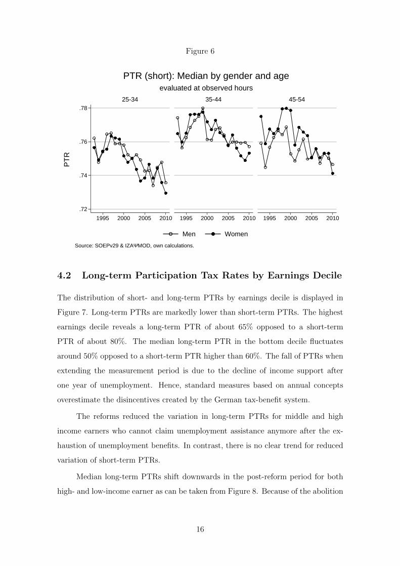
Figure 6
.72
.74
.76
.78
1995 2000 2005 2010 1995 2000 2005 2010 1995 2000 2005 2010
25-34 35-44 45-54
Men Women
PT
R
Source: SOEPv29 & IZAYMOD, own calculations.
evaluated at observed hours
PTR (short): Median by gender and age
4.2 Long-term Participation Tax Rates by Earnings Decile
The distribution of short- and long-term PTRs by earnings decile is displayed in
Figure 7. Long-term PTRs are markedly lower than short-term PTRs. The highest
earnings decile reveals a long-term PTR of about 65% opposed to a short-term
PTR of about 80%. The median long-term PTR in the bottom decile fluctuates
around 50% opposed to a short-term PTR higher than 60%. The fall of PTRs when
extending the measurement period is due to the decline of income support after
one year of unemployment. Hence, standard measures based on annual concepts
overestimate the disincentives created by the German tax-benefit system.
The reforms reduced the variation in long-term PTRs for middle and high
income earners who cannot claim unemployment assistance anymore after the ex-
haustion of unemployment benefits. In contrast, there is no clear trend for reduced
variation of short-term PTRs.
Median long-term PTRs shift downwards in the post-reform period for both
high- and low-income earner as can be taken from Figure 8. Because of the abolition
16

Figure 7
-.5
0
.5
1
1 2 3 4 5 6 7 8 9 10 1 2 3 4 5 6 7 8 9 10
PTR (short) PTR (long)
1995 2006
PT
R
Source: SOEPv29 & IZAYMOD, own calculations.
evaluated at observed hours
PTR across earnings deciles
of unemployment assistance in 2005 income may drop even further to levels of social
assistance if the individual is the household’s principal earner. Accordingly, the
post-reform spread between short-term and long-term PTRs increases to almost 20
percentage points for most deciles. As for short-term PTRs, observed median PTR
of women falls the most over the reform period from 40–50% to about 30%.
The drop of long-term PTRs is even more distinct for median PTRs by gender
and age as presented in Figure 9. Particularly for the young, the median PTR drops
from about 65% to about 55%.
17

Figure 8
.3
.4
.5
.6
.7
.3
.4
.5
.6
.7
1995 2000 2005 2010 1995 2000 2005 2010 1995 2000 2005 2010
Men, observed hours Men, 20 hours Men, 40 hours
Women, observed hours Women, 20 hours Women, 40 hours
Decile 1 Decile 5 Decile 10
PT
R
Source: SOEPv29 & IZAYMOD, own calculations.
PTR (long): Median by earnings deciles
Figure 9
.55
.6
.65
.7
1995 2000 2005 2010 1995 2000 2005 2010 1995 2000 2005 2010
25-34 35-44 45-54
Men Women
PT
R
Source: SOEPv29 & IZAYMOD, own calculations.
evaluated at observed hours
PTR (long): Median by gender and age
18

Figure 10
.4
.5
.6
0 5 10 0 5 10
1995 2006
Baseline Scenario 1
PT
R
Decile
Source: SOEPv29 & IZAYMOD, own calculations.
evaluated at observed hours
Median PTR (long) with human capital depreciation 1
4.3 Participation Tax Rates with Human Capital Depreci-
ation by Earnings Decile
PTRs by earnings decile accounting for human capital depreciation is presented in
Figures 10 and 11. PTRs of scenario 1 in Figure 10 are compared to the sum of the
second and third component of a three-year PTR. PTRs of scenario 2 in Figure 11
are compared to the third component of a three-year PTR. Including human capital
depreciation decreases the PTR in both scenarios compared to the baseline scenario.
PTRs based on the human capital depreciation scenarios are lower because
taxes on depreciated earnings are lower and benefit eligibility after a period of unem-
ployment is reduced. Lost eligibility for unemployment benefits and unemployment
assistance explains most of the distance between the baseline scenario and human
capital depreciation scenarios before the reforms. The abolishment of unemployment
assistance makes the difference in 2006 almost negligible.
19

Figure 11
.3
.4
.5
.6
0 5 10 0 5 10
1995 2006
Baseline Scenario 2
PT
R
Decile
Source: SOEPv29 & IZAYMOD, own calculations.
evaluated at observed hours
Median PTR (long) with human capital depreciation 2
4.4 Participation Tax Rates by Household Type
A PTR highly depends on the household context which determines income taxes
paid and transfers received. Figure 12 illustrates how short-term PTRs vary by
a household’s composition of earners. PTRs are highest for two-earner households.
Primary earners face a short-term PTR of about 77% and secondary earners a short-
term PTR of about 84%. Sole earners benefit most from joint taxation being able to
reassert the full splitting advantage and have a PTR of about 70%. Singles’ PTRs of
about 75% lie between those of two-earner households and sole-earner households.
The group of secondary earners is very heterogenous with some earning only slightly
less than the primary earner and others only marginally employed. As a result, PTRs
of secondary earners are more dispersed.
To further investigate the driving forces behind the resulting PTRs, we can
break down its components as follows
PTRih =(tE,inc
h + sEh − bEh )− (tU,inch + sUh − bUh )
yE,wi
, (4)
20

Figure 12
.4
.6
.8
1
1.2
PT
R
1995 2001 2006
Source: SOEPv29 & IZAYMOD, own calculations.
evaluated at observed hours
PTR (short): Distribution by earner type
Single Sole earner Primary earner Secondary earner
where income taxes are tinch , social security contributions are sh and benefits are bh
in labor market states E and U , respectively. Figure 13 gives the median share of
each component by household earner type in pre-reform year 1995 and post-reform
year 2006.
The income tax wedge between E and U dropped from 22% in 1995 to 17% in
2006 on average. Consequently, the fraction of the PTR attributable to income taxes
falls disproportionately. Both singles and sole earners only pay income tax when
employed. Their median income tax share tE,inch /yE,w
i dropped from 18% to 16% for
singles and from 11% to 7% for sole earners who benefit from joint taxation with
a spouse with zero earnings. In contrast, individuals in two-earner households face
higher income tax wedges paying taxes in both labor market states. The median
income tax wedge (tE,inch − tU,inch )/yE,w
i declines from 45% − 22% = 23% in 1995
to 40% − 21% = 19% in 2006 for secondary earners. The basic tax allowance was
raised substantially in the time between such that half of all primary earners are
not subject to income taxes in U in the post-reform period the median income tax
wedge drops from 26%− 1% = 25% in 1995 to 20%− 0% = 20% in 2006.
21

The share of out-of-work benefits bUh /yE,wi decreased on average from 41% to
39%. It declines most strongly for secondary earners from 46% to 43%, whereas all
other groups lost only one percentage point. Individuals living in two-earner house-
holds are subject to the withdrawal of means-tested benefits when household income
exceeds the hypothetical claims. According to the lower level of state support their
PTRs should be lower than for singles which is the case for the UK demonstrated
by Brewer et al. (2008). However, PTRs in Germany are mainly determined by
earnings-related unemployment benefits that do not depend on other household in-
come sources. Additionally, joint taxation creates low income tax shares for sole
earners and higher income tax shares for two-earner households. Secondary earners
have particularly high shares of out-of-work benefits since the share of unemploy-
ment benefits in gross earnings is higher than for other household earner types.
Unemployment benefits are 60% of previous net earnings for childless persons and
67% for parents, where net earnings are gross earnings reduced by income tax on
the respective earnings abstracting from other income sources and social security
contributions. The respective average income tax is lower for low-income earners in
a progressive income tax system as in Germany. As a result, the share of unemploy-
ment benefits in gross earnings is higher for low-income secondary earners.
In sum, we have identified three main drivers of PTRs in Germany. Eligibility
for unemployment benefits, which is amongst others determined by the social se-
curity earnings threshold, is the most important institutional factor behind a high
PTR. The number of earners in the household mainly determines the tax wedge
between E and U because of the extent to which joint taxation reduces the house-
hold’s tax burden in both states. Age and earnings potential seem to be the most
relevant individual characteristics determining the size of the PTR.
22

Figure 13
-1
0
1
2
-1
0
1
2
1995 2006 1995 2006
1995 2006 1995 2006
Single Sole earner
Primary earner Secondary earner
Benefits in U SSC in E Taxes in ETaxes in U SSC in U Benefits in E
PT
R
Source: SOEPv29 & IZAYMOD, own calculations.
evaluated at observed hours
Composition of PTR (short)
5 Regression Analysis
Labor market participation in Germany increased substantially during and after the
Hartz reforms at the beginning of the 2000s.10 These reforms also triggered a reduc-
tion in PTRs, i.e., increased work incentives. We thus examine in the following how
strongly changes in the PTRs were related to changes in individuals’ employment
status.
5.1 Estimation Strategy
We test in our regression analysis to which extent lower PTRs are associated with
an increased likelihood of taking up work. The binary outcome variable is one if
individual i switches from non-participation in period t−1 (Uit−1) to participation in
period t (Eit). The main explanatory variable of interest is the PTR-change between
period t − 1 and t, i.e., ∆PTRit = PTRit − PTRit−1. We estimate the following
10See Appendix Figure B.2 for labor market participation in Germany from 1991 to 2012 bygender and age group.
23

regression model:
P (Uit−1 → Eit) = γ∆PTRit +X ′itβ + αi + µt + εit (5)
The coefficient γ captures the effect of a PTR-change on the likelihood of taking up
work and is expected to be negative, i.e., a decrease (increase) is associated with
a higher (lower) likelihood of labor market participation. Controls are captured by
Xit and include age, household type, region and state-specific unemployment rates.
Year fixed effects capture business cycle fluctuations affecting labor demand and are
denoted by µt. The error term is denoted by εit. We estimate this equation with
ordinary least squares (OLS) and in an individual fixed effects (FE) framework ex-
ploiting individual variation around an individual time-invariant fixed effect denoted
by αi, which captures unobserved heterogeneity, such as preferences for leisure or
innate ability affecting the employment status. In addition, we include interactions
of the change in PTR with age groups and the unemployment rate in order to test
for heterogeneous effects for younger and older workers and whether the incentive
effect from the PTR is affected by regional labor market conditions. All estimations
are conducted separately for men and women.
A transition from U to E is only observed in the sample if we include those
in U as well. Hence, we make use of the simulated earnings for 20 and 40 hours
of work for all individuals in the work force independent of their observed labor
market status. For the regression analysis, we use PTRs obtained on the basis of
these simulated earnings. As discussed in Section 4, we obtain rather similar PTRs
with all three simulation scenarios, but slightly overestimate PTRs at the bottom of
the earnings distribution when using simulated earnings because of the fixed hours
(20 or 40) assumption. In sum, we apply four PTR concepts as independent variable:
short- and long-term PTRs each evaluated at 20 or 40 weekly working hours.
5.2 Estimation Results
Regression results are presented in Tables 1–4. The results for the effect of short-
term PTRs are displayed in Tables 1 and 2. Overall, we find that a reduction in the
24
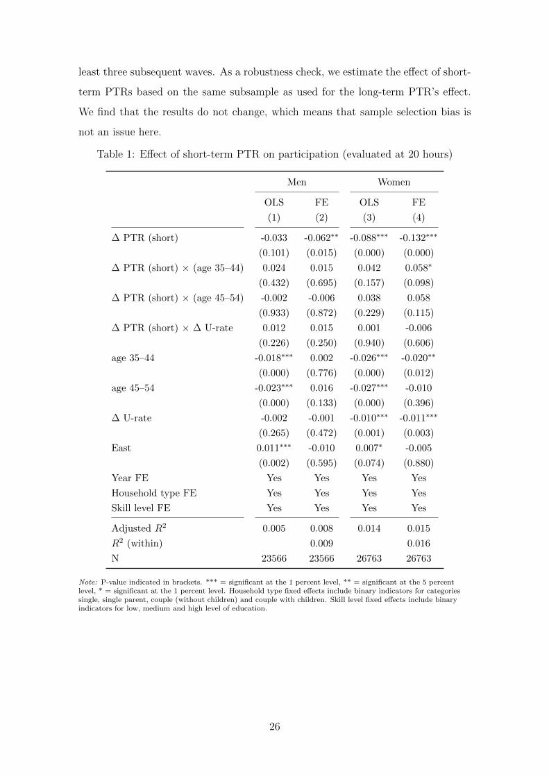
PTR has a positive and statistically significant effect on the likelihood of taking up
a job with stronger effects for women. This coincides with the empirical result that
women are more responsive at the extensive margin than men. The individual fixed
effects model obtains bigger effects as can be taken from a comparison of the OLS
results in columns (1) for men and (3) for women with the individual fixed effects
results in columns (2) and (4), respectively.11 This suggests that unobserved and
time-invariant determinants such as different taste for work or leisure exist and OLS
results suffer from heterogeneity bias.
The impact of the short-term PTR on the probability to take up work is
also economically significant. E.g., reducing the PTR by ten percentage points
increases the probability of taking up work by 0.6–0.9 (1.3–1.5) percentage points
for men (women) depending on whether the PTR is evaluated at 20 or 40 hours per
week, respectively. Given the baseline probabilities about three (four) percent for
men (women) shown in Figure 1 this is quite substantial in magnitude. It means
that policy reforms aiming at increasing work incentives have a sizable impact on
employment. Considering heterogeneity across age, we do not find that this result
varies significantly across age groups. The only slight exception is found for women
where the effect of a change in the short-term PTR is somewhat less pronounced for
women of older age compared to the youngest age group between 25 and 34. The
estimates of the interaction terms are however only marginally significant if at all.
The results for the effect of long-term PTRs are displayed in Tables 3 and 4.
In general, we find that reductions in the long-term PTR also have a positive impact
on the job-take-up probability. The results are slightly smaller in magnitude, by and
large around −0.1 for both men and women, which again implies a one percentage
point increase in switching to employment for a ten percentage point reduction in
the PTR. The results for long-term PTRs are however less precisely estimated and
even turn statistically insignificant at conventional levels when being evaluated at
40 hours. The sample size for the estimation of the effect of long-term PTRs is
substantially reduced since we have to rely on individuals who are surveyed for at
11We also estimated the regression model using a logit specification with and without individualfixed effects. The results are qualitatively very similar to the results from the linear probabilitymodel. The results are presented in Tables C.1–C.4 in the Appendix.
25
least three subsequent waves. As a robustness check, we estimate the effect of short-
term PTRs based on the same subsample as used for the long-term PTR’s effect.
We find that the results do not change, which means that sample selection bias is
not an issue here.
Table 1: Effect of short-term PTR on participation (evaluated at 20 hours)
Men Women
OLS FE OLS FE
(1) (2) (3) (4)
∆ PTR (short) -0.033 -0.062∗∗ -0.088∗∗∗ -0.132∗∗∗
(0.101) (0.015) (0.000) (0.000)
∆ PTR (short) × (age 35–44) 0.024 0.015 0.042 0.058∗
(0.432) (0.695) (0.157) (0.098)
∆ PTR (short) × (age 45–54) -0.002 -0.006 0.038 0.058
(0.933) (0.872) (0.229) (0.115)
∆ PTR (short) × ∆ U-rate 0.012 0.015 0.001 -0.006
(0.226) (0.250) (0.940) (0.606)
age 35–44 -0.018∗∗∗ 0.002 -0.026∗∗∗ -0.020∗∗
(0.000) (0.776) (0.000) (0.012)
age 45–54 -0.023∗∗∗ 0.016 -0.027∗∗∗ -0.010
(0.000) (0.133) (0.000) (0.396)
∆ U-rate -0.002 -0.001 -0.010∗∗∗ -0.011∗∗∗
(0.265) (0.472) (0.001) (0.003)
East 0.011∗∗∗ -0.010 0.007∗ -0.005
(0.002) (0.595) (0.074) (0.880)
Year FE Yes Yes Yes Yes
Household type FE Yes Yes Yes Yes
Skill level FE Yes Yes Yes Yes
Adjusted R2 0.005 0.008 0.014 0.015
R2 (within) 0.009 0.016
N 23566 23566 26763 26763
Note: P-value indicated in brackets. *** = significant at the 1 percent level, ** = significant at the 5 percentlevel, * = significant at the 1 percent level. Household type fixed effects include binary indicators for categoriessingle, single parent, couple (without children) and couple with children. Skill level fixed effects include binaryindicators for low, medium and high level of education.
26

Table 2: Effect of short-term PTR on participation (evaluated at 40 hours)
Men Women
OLS FE OLS FE
(1) (2) (3) (4)
∆ PTR (short) -0.061∗∗∗ -0.093∗∗∗ -0.105∗∗∗ -0.151∗∗∗
(0.007) (0.001) (0.000) (0.000)
∆ PTR (short) × (age 35–44) 0.024 0.011 0.038 0.045
(0.496) (0.799) (0.256) (0.280)
∆ PTR (short) × (age 45–54) 0.004 -0.005 0.047 0.067
(0.903) (0.909) (0.187) (0.119)
∆ PTR (short) × ∆ U-rate 0.015 0.019 0.002 -0.006
(0.193) (0.191) (0.797) (0.639)
age 35–44 -0.019∗∗∗ 0.002 -0.025∗∗∗ -0.020∗∗
(0.000) (0.772) (0.000) (0.014)
age 45–54 -0.023∗∗∗ 0.016 -0.027∗∗∗ -0.010
(0.000) (0.140) (0.000) (0.392)
∆ U-rate -0.002 -0.001 -0.010∗∗∗ -0.010∗∗∗
(0.271) (0.500) (0.001) (0.005)
East 0.011∗∗∗ -0.012 0.008∗ -0.006
(0.003) (0.526) (0.067) (0.857)
Year FE Yes Yes Yes Yes
Household type FE Yes Yes Yes Yes
Skill level FE Yes Yes Yes Yes
Adjusted R2 0.006 0.010 0.014 0.016
R2 (within) 0.012 0.017
N 23566 23566 26763 26763
Note: P-value indicated in brackets. *** = significant at the 1 percent level, ** = significant at the 5 percentlevel, * = significant at the 1 percent level. Household type fixed effects include binary indicators for categoriessingle, single parent, couple (without children) and couple with children. Skill level fixed effects include binaryindicators for low, medium and high level of education.
27
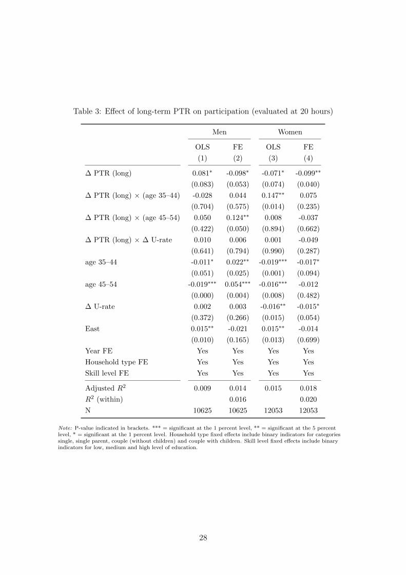
Table 3: Effect of long-term PTR on participation (evaluated at 20 hours)
Men Women
OLS FE OLS FE
(1) (2) (3) (4)
∆ PTR (long) 0.081∗ -0.098∗ -0.071∗ -0.099∗∗
(0.083) (0.053) (0.074) (0.040)
∆ PTR (long) × (age 35–44) -0.028 0.044 0.147∗∗ 0.075
(0.704) (0.575) (0.014) (0.235)
∆ PTR (long) × (age 45–54) 0.050 0.124∗∗ 0.008 -0.037
(0.422) (0.050) (0.894) (0.662)
∆ PTR (long) × ∆ U-rate 0.010 0.006 0.001 -0.049
(0.641) (0.794) (0.990) (0.287)
age 35–44 -0.011∗ 0.022∗∗ -0.019∗∗∗ -0.017∗
(0.051) (0.025) (0.001) (0.094)
age 45–54 -0.019∗∗∗ 0.054∗∗∗ -0.016∗∗∗ -0.012
(0.000) (0.004) (0.008) (0.482)
∆ U-rate 0.002 0.003 -0.016∗∗ -0.015∗
(0.372) (0.266) (0.015) (0.054)
East 0.015∗∗ -0.021 0.015∗∗ -0.014
(0.010) (0.165) (0.013) (0.699)
Year FE Yes Yes Yes Yes
Household type FE Yes Yes Yes Yes
Skill level FE Yes Yes Yes Yes
Adjusted R2 0.009 0.014 0.015 0.018
R2 (within) 0.016 0.020
N 10625 10625 12053 12053
Note: P-value indicated in brackets. *** = significant at the 1 percent level, ** = significant at the 5 percentlevel, * = significant at the 1 percent level. Household type fixed effects include binary indicators for categoriessingle, single parent, couple (without children) and couple with children. Skill level fixed effects include binaryindicators for low, medium and high level of education.
28
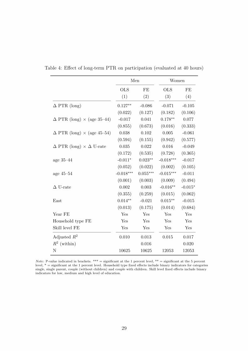
Table 4: Effect of long-term PTR on participation (evaluated at 40 hours)
Men Women
OLS FE OLS FE
(1) (2) (3) (4)
∆ PTR (long) 0.127∗∗ -0.086 -0.071 -0.105
(0.022) (0.127) (0.182) (0.106)
∆ PTR (long) × (age 35–44) -0.017 0.041 0.178∗∗ 0.077
(0.855) (0.673) (0.016) (0.333)
∆ PTR (long) × (age 45–54) 0.038 0.102 0.005 -0.061
(0.594) (0.155) (0.942) (0.577)
∆ PTR (long) × ∆ U-rate 0.035 0.022 0.016 -0.049
(0.172) (0.535) (0.728) (0.365)
age 35–44 -0.011∗ 0.023∗∗ -0.018∗∗∗ -0.017
(0.052) (0.022) (0.002) (0.105)
age 45–54 -0.018∗∗∗ 0.055∗∗∗ -0.015∗∗∗ -0.011
(0.001) (0.003) (0.009) (0.494)
∆ U-rate 0.002 0.003 -0.016∗∗ -0.015∗
(0.355) (0.259) (0.015) (0.062)
East 0.014∗∗ -0.021 0.015∗∗ -0.015
(0.013) (0.175) (0.014) (0.684)
Year FE Yes Yes Yes Yes
Household type FE Yes Yes Yes Yes
Skill level FE Yes Yes Yes Yes
Adjusted R2 0.010 0.013 0.015 0.017
R2 (within) 0.016 0.020
N 10625 10625 12053 12053
Note: P-value indicated in brackets. *** = significant at the 1 percent level, ** = significant at the 5 percentlevel, * = significant at the 1 percent level. Household type fixed effects include binary indicators for categoriessingle, single parent, couple (without children) and couple with children. Skill level fixed effects include binaryindicators for low, medium and high level of education.
29

6 Conclusions
This paper investigates incentives to take up work inherent in the German tax-
benefit system measured by Participation Tax Rates (PTR). Based on rich micro-
data as well as a detailed tax-benefit simulation model for Germany, we provide
extensive descriptive evidence for the trends of the PTR over the period 1993–2010
across the entire earnings distribution as well as for population subgroups like gen-
der, age and household earner type. Moreover, we extend the standard definition
of the (short-term) PTR to a longer time horizon, taking into account that indi-
viduals currently not in employment may have a longer-term perspective on their
participation decision.
Our descriptive results show that long-term PTRs are significantly lower than
short-term PTRs. Three-year PTRs vary between 50% and 65% depending on the
earnings level, whereas short-term PTRs based on a one-year period are between
70% and 80%. Work incentives are higher if the time horizon is extended to more
than one year. Hence, standard measures overestimate the disincentives created by
the German tax-benefit system.
We have identified three main drivers of PTRs in Germany. Eligibility for
unemployment benefits, which is amongst others determined by the social security
earnings threshold, is the most important institutional factor behind a high PTR.
Low-income earner face particularly low PTRs not being eligible for unemployment
benefits. The number of earners in the household mainly determines the tax wedge
between E and U because of the extent to which joint taxation reduces the house-
hold’s tax burden in both states. Age and earnings potential seem to be the most
relevant individual characteristics. PTRs are lower for younger age groups and for
sole earners who benefit most from joint taxation.
Germany’s tax and labor market reforms in the early 2000s substantially re-
duced PTRs, particularly for low-income earners. Our regression analysis reveals
that a PTR reduction indeed increases the likelihood of taking up work significantly,
particularly for women. Hence, improved work incentives most likely contributed to
the observed increase in labor market participation in the aftermath of the reforms
in Germany. Finally, the work incentive measure derived from optimal tax theory
30

seems to have empirical relevance for observed labor supply decisions.
31

References
Adam, S., M. Brewer, and A. Shephard (2006). The poverty trade-off. Work incen-tives and income redistribution in Britain. Policy Press.
Bonke, T. and S. Eichfelder (2010). Horizontal equity in the German tax-benefitsystem: A simulation approach for employees. FinanzArchiv - Public FinanceAnalysis 66, 295–331.
Brewer, M., E. Saez, and A. Shephard (2008). Means-testing and tax rates onearnings. Prepared for the Report of a Commission on Reforming the Tax Systemfor the 21st Century, Chared by Sir James Mirrlees, Institute for Fiscal Studies.
Chetty, R., A. Guren, D. Manoli, and A. Weber (2013). Does Indivisible LaborExplain the Difference between Micro and Macro Elasticities? A Meta-Analysisof Extensive Margin Elasticities. NBER Macroeconomics Annual 2012 27, 1–56.
Corneo, G. (2005). Verteilungsarithmetik der rot-grunen Steuerreform. SchmollersJahrbuch - Journal of Applied Social Science Studies 125, 299–314.
Diamond, P. (1980). Income Taxation with Fixed Hours of Work. Journal of PublicEconomics 13, 101–110.
Dockery, A., R. Ong, and G. Wood (2011). Welfare Traps in Australia: Do theybite? CLMR Discussion Papier Series No. 08/02.
Gregory, M. and R. Jukes (2001). Unemployment and Subsequent Earnings: Esti-mating Scarring among British Men 1984-94. The Economic Journal 111, F607–F625.
Heckman, J. (1979). Sample Selection Bias as a Specification Error. Economet-rica 47, 153–161.
Immervoll, H., H. Kleven, C. Kreiner, and E. Saez (2007). Welfare reform in Euro-pean countries: a microsimulation analysis. The Economic Journal 117, 1–44.
Immervoll, H., H. Kleven, C. Kreiner, and N. Verdelin (2009). An Evaluation ofthe Tax-Transfer Treatment of Married Couples in European Countries. IZA-Discussion Paper No. 3965.
Jacquet, L., E. Lehmann, and B. V. der Linden (2013). Optimal redistributivetaxation with both extensive and intensive responses. Journal of Economic The-ory 148, 1770–1805.
Kim, M.-K. and S. Polachek (1994). Panel Estimates of Male-Female EarningsFunctions. The Journal of Human Resources 29 (2), 406–428.
Loffler, M., A. Peichl, N. Pestel, S. Siegloch, and E. Sommer (2014, October). Doc-umentation IZAΨMOD v3.0: The IZA Policy Simulation Model. IZA DiscussionPaper Nr. 8553.
32
Meghir, C. and D. Phillips (2010). Labor Supply and Taxes, Chapter 3 for MirrleesReview (2009). In J. Mirrlees, S. Adam, T. Besley, R. Blundell, S. Bond, R. Chote,M. Gammie, P. Johnson, G. Myles, and J. Poterba (Eds.), Dimensions of TaxDesign: the Mirrlees Review. Oxford University Press.
Mincer, J. and H. Ofek (1982). Depreciation and Restoration of Human Capital.The Journal of Human Resources 17 (1), 3–24.
Mirrlees, J. (1971). An Exploration in the Theory of Optimal Income Taxation.Review of Economic Studies 38, 175–208.
O’Donoghue, C. (2011). Do tax-benefit systems cause high replacement rates? Adecompositional analysis using EUROMOD. LABOUR 25, 126–151.
Pirttilla, J. and H. Selin (2011). Tax Policy and Employment: How does the Swedishsystem fare. CESifo Working Paper Series No. 3355.
Saez, E. (2002). Optimal Income Transfer Programs: Intensive versus ExtensiveLabor Supply Responses. Quarterly Journal of Economics 117, 1039–1073.
Wagner, G., J. Frick, and J. Schupp (2007). The German Socio-Economic PanelStudy (SOEP) - Scope, evolution and enhancements. Schmollers Jahrbuch - Jour-nal of Applied Social Science Studies 127, 139–170.
33

Appendix
A German Tax-Benefit System
A.1 Benefits
Statutory provisions for each of the potential transfer payments are described in thefollowing. Individual in state U are potentially eligible for insurance payments andmeans-tested payments.
A.1.1 Unemployment Benefits
As an insurance program, a potential receipt of unemployment benefits depends oninsurance contributions carried out during employment. Contributions to unem-ployment insurance and thus unemployment benefits are top-coded. Unemploymentbenefits bubi,t(c) in year t are obtained as a specific percentage of net earnings. For thesimulation of unemployment benefits bubi,t(c) hypothetically received if out of workare based on earnings of the current year t. Formally unemployment benefits aregiven by
bubi,t(c) = sub(c) · (ywi,t−1 − twi,t−1 − Si,t−1),
where sub(c) is the percentage of previous net earnings depending on the existenceof children c ∈ {0, 1}. sub(c) lies at 60% for childless individuals (c = 0) and at 67%for parents (c = 1). Net earnings are given by gross earnings ywi,t reduced by wagetaxes twi,t and social security contributions Si,t.
In order to be eligible for unemployment benefits a person has to have a recordof employment subject to social security contributions for at least one year within thelast three years (1982-2005) or within the last two years (2006-today). Marginallyemployed do not contribute to unemployment insurance and are thus not eligible.
The entitlement length depends on the number of months employed subject tosocial security contributions during the last seven or five years, respectively. For thesimulation it is assumed, that individuals eligible for unemployment benefits wereemployed in total for at least 24 months during the last seven years (1987-2005) orfive years (2006-today), respectively, thus being eligible for 12 months unemploy-ment benefits. The length of entitlement is increasing with age. We refrain fromincreasing unemployment benefit length with age since most of the age-dependentvariation applies do older employees not part of our sample anyway.
A.1.2 Unemployment Assistance
Until 2005, individuals may receive earnings-related unemployment assistance afterthe exhaustion of unemployment benefits. Unemployment assistance is an insurancepayment hinging on social security contributions, but means-tested at the same time.Possible claims for unemployment assistance are reduced by net household income.Net household income is reduced again by an allowance on spouse’s earnings equal to
34

his hypothetical unemployment assistance claim. The remaining amount decreasesthe claim of the individual for unemployment assistance which can be expressed as
buai,t (c) = sua(c) · (ywi,t−1 − twi,t−1 − Si,t−1)
−((yUh,t−1 − tUh,t−1 − Sj,t−1)− sua(c) · (ywj,t−1 − twj,t−1 − Sj,t−1)),
where sua(c) is the percentage of previous net earnings depending on the existenceof children c ∈ {0, 1}. sua(c) is at 53% for childless individuals (c = 0) and at 57%for parents (c = 1). ywj,t, t
wj,t and Sj,t are spouse’s earnings, wage taxes and social
security contributions. In sum, only single or individuals with a partner who isa transfer recipient and/or not working receive the full amount of unemploymentassistance. Families with children receive a more generous income support. This isthe case for both unemployment benefits and unemployment assistance. Unemploy-ment assistance is allowed for one year after which the individual has to renew hisclaim and prove his neediness again. Under the condition that the claim is admittedunemployment assistance can be granted until the individual’s retirement.
A.1.3 Social Assistance
Means-tested social assistance is based on the needs of the household as a whole withhousehold members being treated as a community (Bedarfsgemeinschaft). House-holds can be entitled to social assistance if the individual in state U has not con-tributed (sufficiently) to unemployment insurance in state E (1) or if the claimfor unemployment benefits/assistance of the individual in state U is very low (2).In 2005, the Hartz IV -reform merges social assistance for those able to work andunemployment assistance to a single system so-called unemployment benefit II (Ar-beitslosengeld II ). Since payments of unemployment benefit II are equivalent tosocial assistance it is referred to social assistance in the following. Starting in 2005,households additionally can be entitled to social assistance if unemployment benefitsof the individual in state U are exhausted (3) with the overall household income notcovering household needs.
The household head receives the standard rate of social assistance, whereasother household members only receive a share of the standard rate depending onage. Hence, social assistance increases with the number of persons in the house-hold. The sum of household member shares gives the householdsize-specific factorfh,t which is multiplied by the annual standard rate srh,t(r). The standard ratesrh,t(r) differs by region r the household is located (West or East Germany) andyear t. Additionally, housing assistance hhh,t(r) is provided to compensate for rentand heating payments. Possible claims on social assistance bsah,t(c) are computed as
bsah,t(c) = fh,t · srh,t(r) + hhh,t(r)
Potential claims for social assistance are reduced by household income andproperty as well as unemployment benefits and unemployment assistance. For thesimulation it is assumed that household’s property does not exceed the exemptionlimits. Following Bonke and Eichfelder (2010), claims for social assistance after de-
35

ductions can be expressed as
bsah,t(c) = Max(fh,t · srh,t(r) + hhh,t(r)− chh,t(c)−Max(yUh − tUh + bubi,t(c) + buai,t (c)−Min(LE, yUh )− Aj, 0), 0),
where chh,t(c) are child benefits and Aj denotes the earnings allowance for spousej’s earnings ywj,t. LE is lump-sum income-related expenses of 100 Euro per month or1,200 per year, which is granted since 2005. Statutory earnings allowance are sub-ject to reform between the two three-year periods. Allowances 1995-1997 are given as
Aj,t =
ywj,t if ywj,t ≤ 0, 25 · srh,t(r)0.25 · srh,t(r) + 0.15 · (ywj,t − 0.25 · srh,t(r)) if 0.25 · srh,t(r) < ywj,t0.25 · srh,t(r) + 0.15 · (ywj,t − 0.25 · srh,t(r)) if ≤ 0.5 · srh,t(r)
Allowances since 2005 are defined as
Aj,t =
0.2 · (ywj,t − 1, 200) if 1, 200 < ywj,t ≤ 9, 600
0.2 · 8, 400 + 0.1 · (ywj,t − 9, 600) if 9, 600 < ywj,t ≤ 14, 400
0.2 · 8, 400 + 0.1 · 8, 400 if ywj,t > 14, 400
The upper limit of 14,400 Euro increases to 18,000 Euro if children live in the house-hold.
A.1.4 Housing allowance
Households with an income below a specific threshold can apply for housing al-lowance instead of social assistance. The payment depends on the number of house-hold members and on household income reduced by lump sum deductions. Housingallowances are computed in accordance to the German Housing Benefit Act (Wohn-geldgesetz ) following Bonke and Eichfelder (2010) as
bhah,t = Max(Hhah,t − (ai + bi ·Hha
h,t + ci ·Hhah,t) · yhah,t, 0),
where Hhah denotes the relevant housing costs, yhah the relevant net household income
and ai, bi, ci the factors in appendix 1 of the Housing Benefit Act. The relevantincome for housing benefits yhah is gross household income yUh reduced by the lumpsum for income-related expenses LE. The relevant housing costs Hha
h,t are calculatedequivalently to housing assistance as included in social assistance.
A.1.5 Child benefits
Households with children receive child benefits depending on the number of chil-dren. Child benefits are paid at least until the 18th birthday regardless of the labormarket state of the parents. A tax exemption instead of child benefits is granted tohouseholds with higher income. In 2005 an additional child benefit (Kinderzuschlag)is introduced to raise the household income of working families above the threshold
36

of social assistance. The additional child benefit is conditional on being employedand is so far the only in-work benefit in Germany. Households are eligible for thisbenefit if household income meets the needs of the parents but not the needs oftheir children. The maximum benefit lies at 140 Euro per month for children under18 years living in the same household as their parents and is granted to householdswhere household income is equal to the hypothetical claim on social assistance of theparents only. If income lies above that level, additional child benefit is withdrawnat a rate of 70%. The upper income level for eligibility lies at the social assistancelevel for the household as a whole including the children.
A.2 Taxes
Statutory provisions for the calculation of household income taxes and social securitycontributions are described below.
A.2.1 Social security contributions
Individual gross earnings is the assessment basis for social security contributionsof the employee. Earnings below a threshold are denoted as marginal employmentand exempted from social security contributions. The reform in 2003 increases thethreshold remarkably from 325 to 400 Euro per month (or 4,800 Euro annually). Upto the earnings threshold the employer pays a flat-rate contribution which does notestablish an entitlement to social security payments such as unemployment benefitsfor the employee.
Earnings exceeding these thresholds are due to social security contributions re-sulting in high marginal tax rates. With the introduction of a zone with increasingsocial security contributions for modest incomes in 2005 marginal tax rates for lowincome earners are cut down. Since then, social security contributions increase forannual earnings between e1
t=4,800 and e2t=9,600 Euro (so-called Midi-Jobs) from
about 4% to about 21%. The overall social security contribution rate does not varysignificantly over time. Hence, a contribution rate s = 21% is applied to calcu-late social security contributions Sj,t for earnings above earnings threshold e1
t = e2t
between 1995 and 1997 and above e2t between 2005 and 2007, respectively. Above
the contribution ceiling RV Bmaxt of the respective year t contributions are fixed in
absolute value. Social security contributions are simulated for a working spouse jwhen individual i is out of work and in state U . Sj,t are given as
Sj,t =
0 if e1
t > ywj,t
s · (F · e1t + (2− F )(ywj,t − e1
t )) if e1t < ywj,t < e2
t
s · ywj,t if ywj,t > e2t
s ·RV Bmaxt if ywj,t > RV Bmax
t
F is a fixed factor equal to 0.7673.
37

A.2.2 Income tax
Gross household income is subject to taxes on income if exceeding the exemptionlimits. Income tax reforms undertaken by the red-green government between 1998and 2005 reduces average tax rates substantially. The tax burden for low incomegroups is reduced by decreasing the basic allowance and the minimal marginal taxrate. In the German tax schedule, marginal tax rates increase linearly with incomeup to a threshold. The top marginal tax rate stays constant for income exceedingthat threshold. Both threshold and top marginal tax rate are decreased throughoutthe reforms reducing the tax burden of high income groups, too. In 2007, taxableincomes exceeding 250.731 Euro are subject to a marginal tax rate of 45%. Calcu-lating the taxable income, a lump sum for income-related expenses LE and a lumpsum for special private expenses (Sonderausgaben) LS is deducted. It is assumedthat expenses do not exceed these lump-sum deductions. Furthermore, the saver’sallowance SA is deducted from asset income which is twice as high for marriedcouples.
Moreover, social security contributions can be partially deducted from taxableincome. A time-varying amount SEm2
j,t reflecting social security contributions is de-ducted from taxable income. Since 2005 tax authorities apply the more favorableof two different calculations of deductions SEm1
j,t and SEm2j,t (§10 Income Tax Code).
Furthermore, the profit share (Ertragsanteil) of social security pensions is addedto taxable income. Following Bonke and Eichfelder (2010) the taxable base can bedescribed as
yTh,t = yUh,t − LE − LS −Min(Max(SEm1j,t , SE
m2j,t ), Sj,t)
The income tax T inc is then computed according to §32a Income Tax Code. The
income tax rate tinch,t is calculated by tinch,t =T inch,t
yTPh,t
and is applied to the taxable income.
The resulting income tax T inch,t is given by T inc
h,t = tinch,t ·yTh,t. Married couples are taxedjointly. Couple’s joint taxable income is halved to assess the income tax rate. Then,the resulting income tax is doubled.
A.2.3 Solidarity surcharge
A solidarity surcharge T S is levied if the income tax surpasses the exemption limitELS. On the first pay level the surcharge is imposed at a higher marginal ratets∗ = 20%. Hence, T S
h,t is given by
T Sh,t =
{0 if T inc
h,t ≤ ELSt
Min(T inch,t · (1 + ts), T inc
h,t + (T inch,t − ELS
t ) · ts∗) if T inch,t > ELS
t
38

B Additional Figures
Figure B.1
0
2000
4000
6000
1995 2000 2005 2010 1995 2000 2005 2010
Men Women
D1 D2 D3 D4 D5 D6 D7 D8 D9
Cur
rent
Eur
os
Source: SOEPv29 & IZAYMOD, own calculations.
Earnings decile intervals
39

Figure B.2
.6
.7
.8
.9
.6
.7
.8
.9
1990 1995 2000 2005 2010 1990 1995 2000 2005 2010 1990 1995 2000 2005 2010
age 25-29 age 30-34 age 35-39
age 40-44 age 45-49 age 50-54
Men Women
Em
ploy
men
t rat
e
Source: German Microcensus.Note: Vertical line indicates year of major labor market reform (Hartz IV) in 2005.
Employment in Germany, 1991-2012
C Additional Tables
40

Table C.1: Effect of short-term PTR on participation (evaluated at 20 hours)
Men Women
LOGIT LOGIT FE LOGIT LOGIT FE
(1) (2) (3) (4)
∆ PTR (short) -0.834∗∗∗ -0.887∗∗∗ -1.907∗∗∗ -1.844∗∗∗
(0.000) (0.000) (0.000) (0.000)
∆ PTR (short) × (age 35-44) 0.410∗∗∗ 0.130∗∗∗ 0.597∗∗∗ 0.744∗∗∗
(0.000) (0.000) (0.000) (0.000)
∆ PTR (short) × (age 45-54) -1.002∗∗∗ -0.401∗∗∗ 0.262∗∗∗ 0.755∗∗∗
(0.000) (0.000) (0.000) (0.000)
∆ PTR (short) × ∆ U-rate 0.266∗∗∗ 0.230∗∗∗ -0.141∗∗∗ -0.014∗∗∗
(0.000) (0.000) (0.000) (0.000)
age 35-44 -0.574∗∗∗ -0.185∗∗∗ -0.580∗∗∗ -0.611∗∗∗
(0.000) (0.000) (0.000) (0.000)
age 45-54 -0.779∗∗∗ 0.313∗∗∗ -0.654∗∗∗ -0.354∗∗∗
(0.000) (0.000) (0.000) (0.000)
∆ U-rate -0.038∗∗∗ -0.043∗∗∗ -0.183∗∗∗ -0.114∗∗∗
(0.000) (0.000) (0.000) (0.000)
East 0.374∗∗∗ -0.417∗∗∗ 0.174∗∗∗ -0.132∗∗∗
(0.000) (0.000) (0.000) (0.000)
Year FE Yes Yes Yes Yes
Household type FE Yes Yes Yes Yes
Skill level FE Yes Yes Yes Yes
Pseudo-R2 0.024 0.075 0.040 0.073
N 1.02e+08 2959 1.08e+08 4208
Note: P-value indicated in brackets. *** = significant at the 1 percent level, ** = significant at the 5 percentlevel, * = significant at the 1 percent level. Household type fixed effects include binary indicators for categoriessingle, single parent, couple (without children) and couple with children. Skill level fixed effects include binaryindicators for low, medium and high level of education.
41

Table C.2: Effect of short-term PTR on participation (evaluated at 40 hours)
Men Women
LOGIT LOGIT FE LOGIT LOGIT FE
(1) (2) (3) (4)
∆ PTR (short) -1.613∗∗∗ -1.432∗∗∗ -2.221∗∗∗ -1.964∗∗∗
(0.000) (0.000) (0.000) (0.000)
∆ PTR (short) × (age 35-44) 0.049∗∗∗ 0.012 0.310∗∗∗ 0.378∗∗∗
(0.004) (0.259) (0.000) (0.000)
∆ PTR (short) × (age 45-54) -1.180∗∗∗ -0.339∗∗∗ 0.302∗∗∗ 0.806∗∗∗
(0.000) (0.000) (0.000) (0.000)
∆ PTR (short) × ∆ U-rate 0.294∗∗∗ 0.392∗∗∗ -0.144∗∗∗ -0.050∗∗∗
age 35-44 -0.573∗∗∗ -0.209∗∗∗ -0.577∗∗∗ -0.606∗∗∗
(0.000) (0.000) (0.000) (0.000)
age 45-54 -0.800∗∗∗ 0.269∗∗∗ -0.650∗∗∗ -0.342∗∗∗
(0.000) (0.000) (0.000) (0.000)
(0.000) (0.000) (0.000) (0.000)
∆ U-rate -0.030∗∗∗ -0.031∗∗∗ -0.182∗∗∗ -0.111∗∗∗
(0.000) (0.000) (0.000) (0.000)
East 0.369∗∗∗ -0.489∗∗∗ 0.179∗∗∗ -0.129∗∗∗
(0.000) (0.000) (0.000) (0.000)
Year FE Yes Yes Yes Yes
Household type FE Yes Yes Yes Yes
Skill level FE Yes Yes Yes Yes
Pseudo-R2 0.028 0.083 0.042 0.074
N 1.02e+08 2959 1.08e+08 4208
Note: P-value indicated in brackets. *** = significant at the 1 percent level, ** = significant at the 5 percentlevel, * = significant at the 1 percent level. Household type fixed effects include binary indicators for categoriessingle, single parent, couple (without children) and couple with children. Skill level fixed effects include binaryindicators for low, medium and high level of education.
42

Table C.3: Effect of long-term PTR on participation (evaluated at 20 hours)
Men Women
LOGIT LOGIT FE LOGIT LOGIT FE
(1) (2) (3) (4)
∆ PTR (long) 2.540∗∗∗ -3.092∗∗∗ -2.232∗∗∗ -2.460∗∗∗
(0.000) (0.000) (0.000) (0.000)
∆ PTR (long) × (age 35-44) -0.367∗∗∗ 2.727∗∗∗ 5.355∗∗∗ 2.026∗∗∗
(0.000) (0.000) (0.000) (0.000)
∆ PTR (long) × (age 45-54) 4.403∗∗∗ 4.221∗∗∗ -0.445∗∗∗ -0.410∗∗∗
(0.000) (0.000) (0.000) (0.000)
∆ PTR (long) × ∆ U-rate 0.268∗∗∗ -0.527∗∗∗ -0.011∗∗ -1.139∗∗∗
(0.000) (0.000) (0.049) (0.000)
age 35-44 -0.402∗∗∗ 0.915∗∗∗ -0.720∗∗∗ -1.071∗∗∗
(0.000) (0.000) (0.000) (0.000)
age 45-54 -0.922∗∗∗ 2.701∗∗∗ -0.540∗∗∗ -0.926∗∗∗
(0.000) (0.000) (0.000) (0.000)
∆ U-rate 0.081∗∗∗ 0.218∗∗∗ -0.306∗∗∗ -0.196∗∗∗
(0.000) (0.000) (0.000) (0.000)
East 0.557∗∗∗ -18.706 0.534∗∗∗ 0.319∗∗∗
(0.000) (0.978) (0.000) (0.000)
Year FE Yes Yes Yes Yes
Household type FE Yes Yes Yes Yes
Skill level FE Yes Yes Yes Yes
Pseudo-R2 0.054 0.240 0.057 0.159
N 4.80e+07 1005 4.99e+07 1260
Note: P-value indicated in brackets. *** = significant at the 1 percent level, ** = significant at the 5 percentlevel, * = significant at the 1 percent level. Household type fixed effects include binary indicators for categoriessingle, single parent, couple (without children) and couple with children. Skill level fixed effects include binaryindicators for low, medium and high level of education.
43

Table C.4: Effect of long-term PTR on participation (evaluated at 40 hours)
Men Women
LOGIT LOGIT FE LOGIT LOGIT FE
(1) (2) (3) (4)
∆ PTR (long) 3.671∗∗∗ -2.622∗∗∗ -2.273∗∗∗ -2.417∗∗∗
(0.000) (0.000) (0.000) (0.000)
∆ PTR (long) × (age 35-44) 0.571∗∗∗ 2.603∗∗∗ 6.679∗∗∗ 1.867∗∗∗
(0.000) (0.000) (0.000) (0.000)
∆ PTR (long) × (age 45-54) 4.894∗∗∗ 3.089∗∗∗ -0.519∗∗∗ -0.644∗∗∗
(0.000) (0.000) (0.000) (0.000)
∆ PTR (long) × ∆ U-rate 1.181∗∗∗ 0.092∗∗∗ 0.239∗∗∗ -1.379∗∗∗
(0.000) (0.000) (0.000) (0.000)
age 35-44 -0.408∗∗∗ 0.926∗∗∗ -0.714∗∗∗ -1.091∗∗∗
(0.000) (0.000) (0.000) (0.000)
age 45-54 -0.873∗∗∗ 2.778∗∗∗ -0.531∗∗∗ -0.939∗∗∗
(0.000) (0.000) (0.000) (0.000)
∆ U-rate 0.076∗∗∗ 0.200∗∗∗ -0.308∗∗∗ -0.198∗∗∗
(0.000) (0.000) (0.000) (0.000)
East 0.545∗∗∗ -19.055 0.534∗∗∗ 0.309∗∗∗
(0.000) (0.982) (0.000) (0.000)
Year FE Yes Yes Yes Yes
Household type FE Yes Yes Yes Yes
Skill level FE Yes Yes Yes Yes
Pseudo-R2 0.057 0.236 0.057 0.157
N 4.80e+07 1005 4.99e+07 1260
Note: P-value indicated in brackets. *** = significant at the 1 percent level, ** = significant at the 5 percentlevel, * = significant at the 1 percent level. Household type fixed effects include binary indicators for categoriessingle, single parent, couple (without children) and couple with children. Skill level fixed effects include binaryindicators for low, medium and high level of education.
44