Embed Size (px)
Citation preview
The Impact of Multifamily Development on Single Family Home Prices in the Greater Boston Area
By
Arah Schuur
B.S. Biology
Yale University, 1993
Submitted to the Center for Real Estate and the Department of Urban Studies and Planning on May 19, 2005 in Partial Fulfillment of the Requirements for the Degrees of
MASTER OF SCIENCE IN REAL ESTATE DEVELOPMENT
and MASTER IN CITY PLANNING
at the Massachusetts Institute of Technology
© 2005 Arah Schuur. All rights reserved
The author hereby grants to MIT permission to reproduce and to distribute publicly paper and electronic copies of this thesis document in whole or in part.
Signature of Author:.............................................................................................................................
Center for Real Estate and Department of Urban Studies and Planning May 19, 2005
Certified by:.........................................................................................................................................
Henry O. Pollakowski Center for Real Estate
Thesis Supervisor Accepted by:........................................................................................................................................
David Geltner Chairman
Interdepartmental Degree Program in Real Estate Development Accepted by:........................................................................................................................................
Lawrence Vale Director of Master's Program
Department of Urban Studies and Planning
1

2
The Impact of Multifamily Development on Single Family Home Prices in the Greater Boston Area
by
Arah Schuur
Submitted to the Submitted to the Center for Real Estate and the Department of Urban Studies and Planning
on May 19, 2005 in Partial Fulfillment of the requirements for the Degrees of Master of Science in Real Estate Development
and Master in City Planning
ABSTRACT The impact of large, multifamily developments on nearby single-family home prices was tested in five towns in the Greater Boston Area. Case studies that had recent multifamily developments built near transit nodes or town centers were chosen. For each town, a conservative impact zone around the multifamily development was established, and sales prices in this area were compared to those in the rest of the town. Using data on the sales of single-family homes from 1987 until 2005, regression analyses were used to construct hedonic price models for the impact and control areas. This model was used to create a sales price index over time. The trend in the index of the impact zone and the control area was compared in the years immediately preceding the permitting of the multifamily development and the years following completion of the development in order to determine if the multifamily development affected sales prices in the impact zone. In the four cases for which there was appropriate data, no negative effects in the impact zone were found. Thesis Supervisor: Henry O. Pollakowski Title: Research Associate
3

ACKNOWLEDGEMENTS I would like to thank my reader, Professor Terry S. Szold, for her guidance through this process and for her tireless energy and kindness as a teacher and a mentor. She has been an inspiration to me in an academic and professional capacity. Thanks also to my advisor, Henry Pollakowski, for sharing his knowledge and experience in this field. I’d also like to thank my academic advisor, Susan Silberberg, who assuaged my nervousness about returning to school with sound, practical advice. Thanks to my family for their ongoing support of my meandering career path, their eagerness to listen as I discovered this new area of interest, and for all of the newspaper clippings about city planning that they’ve sent over the last two years. Thanks to JJ for always being ready to play the game and to Club 32 for many stress-relieving family nights. Finally, a huge thanks to the Old Ladies for two years of drinks, dinners, and unflagging willingness to listen to me complain!
4
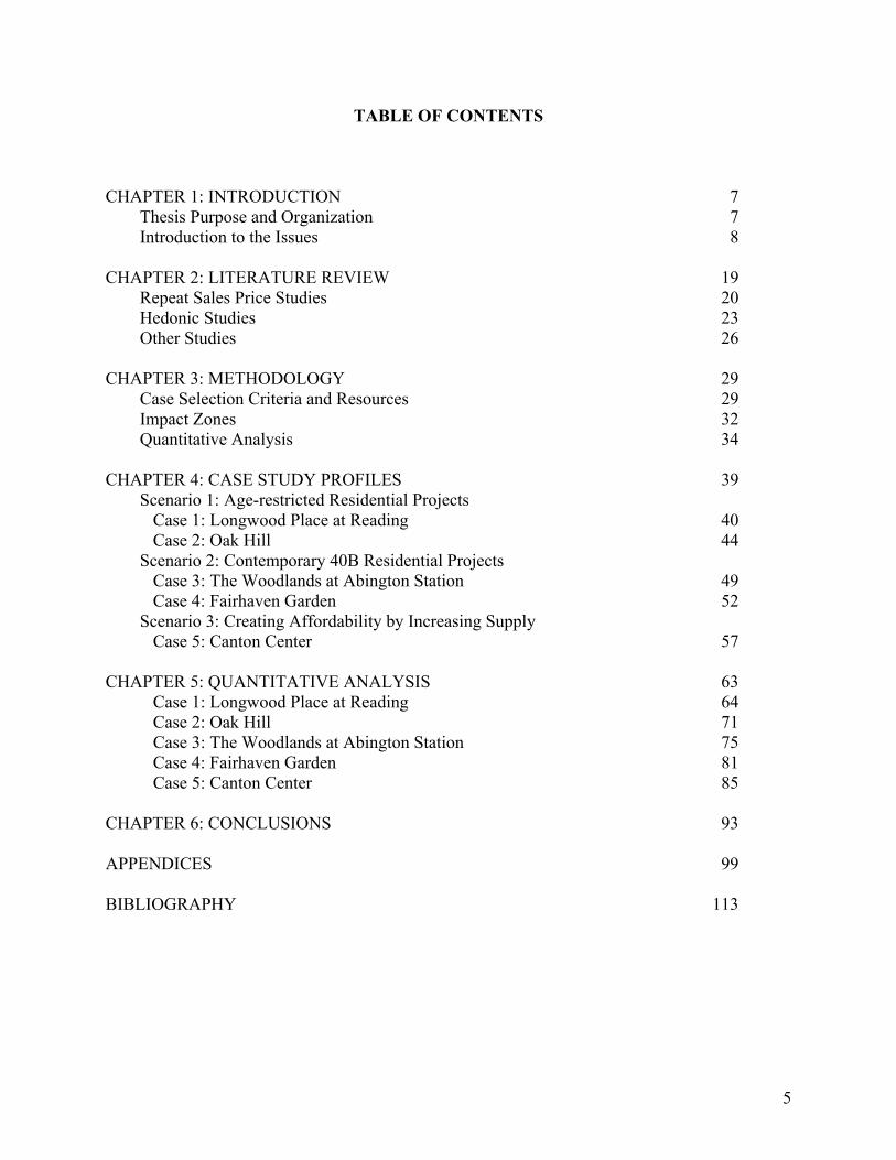
TABLE OF CONTENTS
CHAPTER 1: INTRODUCTION 7 Thesis Purpose and Organization 7 Introduction to the Issues
8
CHAPTER 2: LITERATURE REVIEW 19 Repeat Sales Price Studies 20 Hedonic Studies 23 Other Studies
26
CHAPTER 3: METHODOLOGY 29 Case Selection Criteria and Resources 29 Impact Zones 32 Quantitative Analysis
34
CHAPTER 4: CASE STUDY PROFILES 39 Scenario 1: Age-restricted Residential Projects Case 1: Longwood Place at Reading 40 Case 2: Oak Hill 44 Scenario 2: Contemporary 40B Residential Projects Case 3: The Woodlands at Abington Station 49 Case 4: Fairhaven Garden 52 Scenario 3: Creating Affordability by Increasing Supply Case 5: Canton Center
57
CHAPTER 5: QUANTITATIVE ANALYSIS 63 Case 1: Longwood Place at Reading 64 Case 2: Oak Hill 71 Case 3: The Woodlands at Abington Station 75 Case 4: Fairhaven Garden 81 Case 5: Canton Center
85
CHAPTER 6: CONCLUSIONS
93
APPENDICES
99
BIBLIOGRAPHY 113
5

6

CHAPTER 1: INTRODUCTION
Thesis Purpose and Organization
In this thesis, I investigate the effect of multifamily development on the prices of nearby
single-family homes in five towns in the Greater Boston Area. In the suburban towns that
surround Boston there is strong community opposition to development, specifically the
development of multifamily projects. One of the root causes of this opposition is local
homeowners’ fear that new development will depress the value of their houses. In order to test
the validity of these concerns, I measure the single-family house prices in towns where at least
one multifamily development was planned, permitted, and built. I consider sales prices in the
periods before, during and after the multifamily project was erected in order to determine if the
development had an effect on the trajectory of sales prices of homes around it as compared to the
rest of the town.
This research builds upon previous studies looking at the effect of housing developments
on surrounding single-family homes. Specifically, this thesis extends the work of David Ritchay
and Zoë Weinrobe,1 who studied the impact of large, affordable projects built under
Massachusetts’ Comprehensive Permit Law, commonly known as Chapter 40B. Ritchay and
Weinrobe’s work was the first of its kind to focus on Massachusetts, and in this thesis I seek to
extend their findings to a different type of development. While Ritchay and Weinrobe selected
cases in which large developments were built in low-density, single-family neighborhoods, I
address cases of multifamily developments that have been built near transit nodes, areas with
commercial development, or town centers. I sought case studies that embody certain elements of
Smart Growth planning, such as building near transit and other infrastructure and incorporating a
7
diversity of housing options within a community. Smart Growth is a relatively new and often
nebulously defined term, but it is an important movement in contemporary land use planning,
and has been championed by state-level officials in Massachusetts as the preferred model for
future development. While assessing the success of Smart Growth principles is beyond the
scope of this thesis, I wanted to use case studies that address this movement.
My thesis is organized into six chapters: the introduction in which I introduce some key
theories and ideas, a literature review that examines previous research on the impacts of
affordable and multifamily housing on nearby single-family homes, a description of the case
study developments that I have chosen and the towns that they are in, an explanation of the
methodology that I use for the quantitative analysis, a review of the results of the quantitative
analysis, and a conclusion that addresses both this research and ideas for additional studies on the
topic.
Introduction to the Issues
The Massachusetts Housing Crisis
Housing availability and affordability are among the most pressing issues facing the
Commonwealth of Massachusetts today and the situation in the Greater Boston area is
particularly severe. A 2004 study by the National Low Income Housing Coalition2 determined
that Massachusetts had the second least affordable rents of any state, and the Boston
metropolitan area had the eighth least affordable rents of any U.S. city. According to the 2003
Greater Boston Housing Report Card, rents are increasingly unaffordable3 in the Boston
metropolitan area, with 43.3% of households paying more than 30% of their income for rent, and
21.5% paying more than half of their income.4
8
Buying a home is little better. In 2002, Massachusetts had the third highest median home
price of any state,5 and despite relatively high incomes, had the third highest housing
affordability burden as well.6 The median price of a single-family home in the Greater Boston
area exceeded $400,000 in 2003.7 Again, declining affordability is the trend – in 2003, a
household at the median income could only afford to buy a median priced house in only 70 of the
161 Greater Boston communities, a decrease from 95 communities in 2001 and 149 in 1998.8
The cost of housing is breaking household budgets, changing neighborhoods, and displacing
lower-income and young families. Governor Romney has voiced concerns that high housing
costs may even begin to impact the Commonwealth’s economic competitiveness, as firms
consider relocating to areas with more affordable housing for their workers.
In the most basic economic sense, the skyrocketing housing costs are caused by an
imbalance in housing supply and demand for housing. A relatively strong and diverse economy,
high wages, and quality of life continue to attract households to the Greater Boston Area,
resulting in a strong demand for housing. Between 1990 and 2000 the number of households in
Boston increased by almost 130,000, or 7.7%.9 While the recession has slowed this growth in
the past three years, it is expected that as the economy recovers, and demographic trends such as
immigration and decreasing household size persists, the Greater Boston Area will continue to see
a growth in households. In fact, in 2000 the Census Bureau projected that the Greater Boston
area would see an increase of 100,000 households by the year 2010.10
Meanwhile, the supply of housing, particularly multifamily housing and housing that is
affordable to moderate and low-income households, has not kept pace with this demand. In the
same ten years, from 1990 to 2000, the housing supply only increased by 5%, or 91,567 units,11 a
shortfall of almost 40,000 units. Construction starts, particularly for multifamily housing, are far
9
below the level needed to balance demand. Permits for multifamily units fell from 1970s highs
of about 14,000 units per year to an average of less than 1,500 units per year in the 1990s.12
Land use statistics reinforce this story. Across the Greater Boston Area, land is being developed
seven times faster than the population is growing.13 Residential density is declining across the
state, with persons per acre decreasing from 11.19 in 1950 to 4.97 in 2000.14 These figures
confirm what is visually evident in many of the towns in the Greater Boston area. The new
housing that is being developed is primarily large single-family homes on even larger lots,
expensive, low-density housing that is largely unaffordable to moderate and lower income
households.
The slow pace of multifamily building is not due to a lack of demand – the housing
shortage in the state is widely acknowledged and well documented – but rather by local
reluctance to permit and build multifamily developments. In 2000, Massachusetts ranked 46th
among the 50 states in number of building permits issued. Multifamily permits represented less
than 15% of the total, well below the national average. According to Massachusetts Housing
Partnership, only 28 towns in Massachusetts approved multifamily developments of five or more
units between 2000 and 2002,15 meaning that 90 percent of towns across the state did not
approve a single multifamily development. As of 2001, 45 Massachusetts communities had
implemented growth-rate bylaws that essentially curtailed new construction altogether.16 It is
this widespread resistance to development that exacerbates the housing shortage and drives
housing prices higher and higher.
10
The Homevoter Hypothesis
Behind an alphabet soup of NIMBYs, NOPErs, and BANANAs17 is the disturbing reality
that very little development is occurring in Massachusetts. Indeed, beyond a select few urban
areas, almost no new multifamily housing is being built in the state. As noted above, zoning and
other local land use controls have created this effective development moratorium across the
Greater Boston Area. In many towns, the zoning ordinance prohibits higher-density housing,
and in many cases land use controls effectively rule out all new development.
William Fischel has extended the Homevoter Hypothesis as a means of understanding
this local resistance to development. Land use regulation is a local responsibility, and zoning is
one of the most powerful ways that a town and its residents can control its physical and financial
destiny. Since its earliest days, zoning has been designed to favor the single-family home, and
what Fischel has dubbed the “the primacy of homeownership”18 can be observed from the
position of single-family homes at the top of the use pyramid in most zoning regulations. In
Massachusetts, towns have increasingly favored the single-family designation, and in many
localities, zoning has become a powerful and often-utilized tool for those who seek to restrict
development in their community.
As Fischel details in his book The Homevoter Hypothesis,19 the popularization of the
automobile facilitated a spatial separation of work and live areas, allowing people to drive from
their job to their home, and resulting in the rise of purely residential suburban areas dominated
by single-family homes. The owners of these houses developed into “homevoters;” active
community members who influenced municipal decision making to reflect their own interests.
In the field of land use, homevoters frequently pushed for local regulations and zoning that
restricted development to single-family homes. This has created a self-perpetuating cycle –
11

residential communities ruled by the majority interests of homeowners, who restrict non-
residential development, making the power of homeowners even more concentrated – to the
point where communities are so anti-growth that development has all but halted.
Fischel explains that the homevoters’ anti-development mentality is fundamentally
rational economic decision making. For most people, a home is the largest (and in many cases,
the only) asset that they own. People are ferociously defensive about the value of this asset,
since it represents not only a place to live, but also their personal wealth, their retirement, and
their children’s education and inheritance. However, a home is a high-risk investment. There is
no insurance system for home prices, so homeowners can only protect the value of their asset by
undertaking value maximizing activities, such as home improvement, and resisting value-
minimizing ones.
It is commonly accepted that home values are affected by external factors, including the
amenities and disamenities of the neighborhood and actions, such as tax rate changes, that the
local government takes. In the past thirty years, the dispersion of employment from center cities
to the suburbs has reduced the importance of distance to the central business district in home
prices. Meanwhile, “quality of life,” as measured by such factors as school performance, and
community character, has become a greater factor.
New development brings the potential for many negative impacts on quality of life,
including poor aesthetic design, increased traffic and congestion, burden on schools and public
infrastructure, and a threat to neighborhood character. Homevoters fear this risk of negative
impacts, and worry that new development will decrease their property value, resulting in a
capital loss in their largest asset. In other words, homeowners are aware that if the
neighborhood goes downhill, their home will lose value, so they do everything they can to
12
minimize the chance that their neighborhood will change. Homevoters “…have staked their
savings in their communities’ character”20 and protect it via the blunt but powerful tool of
zoning. Thus, the prevalence of anti-development zoning in many towns can be explained by
homevoters’ financial incentive to protect the value of their homes and their aversion to the risk
inherent in change.
Chapter 40B
The most successful tool that Massachusetts has used to overcome community opposition
to development and to expand the housing supply is a powerful and controversial statute,
Chapter 40B. 40B has been in effect for 36 years and is responsible for the majority of
multifamily and affordable housing in many non-urban communities in the Greater Boston area.
A brief review of the law follows, for more detailed information about Chapters 40B and 40R,
please see the resources listed in the bibliography.
Chapter 40B of the Massachusetts General Law was enacted in 1955. The
Comprehensive Permit Law (Sections 20-23), what is commonly referred to as “40B,” or the
“anti-snob zoning law,” was added in 1969 as a means of encouraging the development of more
affordable housing. This statute created two provisions to facilitate development. First,
developers of projects that include a substantial portion of affordable units can apply to the local
Zoning Board of Appeals (ZBA) for a single comprehensive permit for their project rather than
multiple projects from multiple municipal bodies. Second, in communities where less than ten
percent of the housing stock is deemed affordable, developers whose projects are turned down at
the local level can appeal the decision to a state Housing Appeals Committee, which can overrule
local opposition and approve the project. In practice, the Appeals Committee has supported the
13
development in most cases and Chapter 40B has allowed developers to build large, multifamily
low- or mixed-income projects in many towns with exclusive zoning rules.
Chapter 40B has been the single most successful mechanism in spurring the production
of multifamily housing across the state. In the vast majority of appeals since the enactment of
40B, the state Housing Appeals Committee has found in favor of the developer, and over half of
the developments appealed have been constructed. Since 1969, over 500 developments with
over 35,000 units have been constructed under 40B. In many cases, Chapter 40B is the only way
that these units are being produced. In fact, since 2000, in towns with less than ten percent
affordable units, the comprehensive permit process accounted for almost half the total production
and more than 96 percent of the affordable units produced.21
Chapter 40B has become an increasingly important tool in the production of new
housing. According to the Citizens Housing and Planning Association (CHAPA), the percent of
new units that have been built under 40B has increased from 15% in the early 1970s to 81% in
the mid-1990s. In the past five years, 83% of all affordable units added to the state’s inventory
used the 40B process. 22 These statistics highlight the mounting difficulty of building
multifamily, low- or mixed-income developments in non-urban areas, and the importance of
Chapter 40B in encouraging housing production. Additionally, it is evidence that in looking for
larger multifamily developments in towns in the Greater Boston Area, the vast majority of
examples are projects built under 40B.
Recent changes to 40B have encouraged towns to take a more progressive approach to
planning for housing diversity. For example, a town can now submit a “Planned Production”
plan to the state Department of Housing and Community Development outlining how it will
achieve a minimum 0.75% growth in affordable units each year for five years. If this plan is
14

approved, and the town continues to meet its goals, that town is exempted from state overrides
on 40B projects.
Community Opposition in Massachusetts
Despite its successes, 40B has not had a smooth history. Massachusetts is a home rule
state, with every power not explicitly designated to the Commonwealth reserved for its 361
towns and municipalities. Zoning and land use are among the most cherished of these local
powers, and Chapter 40B has been a particularly passionate subject. The law allows developers,
often viewed as greedy, out-of-town, big-city builders, to surpass local zoning and build
developments that would often not be allowed under the local zoning ordinance. Since its
passage, hundreds of bills proposing to repeal, gut, or weaken Chapter 40B have been filed.
There are innumerable websites dedicated to voicing objections to specific 40B projects or to the
statute itself. The state’s history of multifamily development, low- and mixed-income housing
and 40B projects in particular has been one of intense community opposition.
In public forums such as Town Meeting and ZBA hearings, development is opposed for
its impact on municipal services, school budgets, traffic, and the vague “community character.”
However, in private, motivations are much more aligned with Fischel’s Homevoter Hypothesis.
The anonymous responses to a survey of residents of the town of Dartmouth, Massachusetts
provides compelling evidence to the entrenched antigrowth sentiments in one town. Over half
of the responses to the question “What most threatens the quality of life in Dartmouth?” referred
to development, with such strongly-stated responses as: “I hope you will respond to the need to
slow/stop growth in our beautiful town… No low-income housing… Keep housing
15
developments out... No more development anywhere in town.” Other responses speak to the
fear for home values that is the foundation of the Homevoter Hypothesis:
“Well-defined zoning laws are important along with the protection of property values... If affordable housing is coming, it should be in a rural area not around people whose property values will decrease… I recently moved to Dartmouth and I love it but now there are low income families living in the Capri Motel and that they may be making low-income units in our really good neighborhoods. Things are great right now so why allow people that “may” destroy this? Property values will go down... Zoning for single-family houses to protect property values so as to make the town a desirable community to live in... No low-income housing. It brings property values down… Development of apartment complexes which will lower property values and change Dartmouth from a friendly town into a city environment...”23
If these concerns that residents are voicing are common, then this is evidence that the fear of
property value erosion contributes significantly to the antidevelopment nature of most towns in
the Greater Boston area.
Smart Growth and Chapter 40R
In the summer of 2004, the Massachusetts legislature passed the first new statute since
40B to address the stagnant supply of housing. This law, known as Chapter 40R, attempts to use
a carrot rather than the stick of 40B to encourage new housing development. 40R encourages
municipalities to enact “Smart Growth” overlay districts, and offers financial incentives from the
state for those towns that do create the new districts. Positioned as providing a positive incentive
for development, the statute is intended to not only spur building, but also to encourage Smart
Growth type development rather than the low-density sprawl that has become common in many
towns in the greater Boston area. The overlay districts must have minimum densities that
encourage multifamily development, and are meant to be located around transit nodes, town
centers, and in abandoned industrial areas. Towns that enact these overlay zones will receive a
payment of up to $5,000 per unit zoned and permitted in the new district, and priority on future
16
disbursement of state funds for municipal services. While 40R is very new, and as of early 2005,
no towns had enacted the new overlay district, the statute demonstrates the state government’s
purported commitment to increasing the supply of housing in Smart Growth development
patterns.
Whether or not Chapter 40R will be successful in both jumpstarting and changing the
nature of housing development in Massachusetts is not yet known. However, in
acknowledgement of the state’s focus on higher-density, multifamily development, I chose to
focus this research on existing developments that demonstrate some of the characteristics favored
in Chapter 40R. Planners and developers promote Smart Growth as the obvious and correct way
to develop going forward, but the economic impacts of this type of development have not been
studied extensively. By investigating the effects of developments with certain Smart Growth
characteristics on single-family homes in the surrounding community, I hope to spur this
conversation.
17
1 Ritchay, David, and Weinrobe, Zoë, Fear and Loathing in Massachusetts: Chapter 40B, Community Opposition, and Residential Property Values, MIT Masters Thesis, 2004. 2 National Low Income Housing Coalition, “Out of reach 2004,” http://www.nlihc.org/oor2004/ 3 In general, housing costs are considered affordable if they consume 30% or less of household income. 4 Citizens Housing and Planning Association, “The Greater Boston Housing Report Card 2003,” http://www.chapa.org/HousingRCard2003.pdf 5 Massachusetts Institute for a New Commonwealth, “Home Ownership in Massachusetts: A New Assessment,” http://www.massinc.org/handler.cfm?type=2&target=PolicyBrief3/policy_brief3.html 6 Housing affordability burden is defined as the median house price / median income ratio. According to MassINC, in 2000 Massachusetts’ ratio was 2.92. 7 The Boston Foundation, “Growth: Time to Play an Inside Game,” http://www.tbf.org/tbfgen1.asp?id=1910 8 Citizens Housing and Planning Association, “The Greater Boston Housing Report Card 2003,” http://www.chapa.org/HousingRCard2003.pdf 9 The Boston Foundation, Boston Indicators Project 2002, Section 6.3.1, http://www.tbf.org/indicators/housing/indicators.asp?id=1205&fID=218&fname=Sustainable%20Development 10 Citizens Housing and Planning Association, “The Greater Boston Housing Report Card 2003,” http://www.chapa.org/HousingRCard2003.pdf 11 The Boston Foundation, Boston Indicators Project 2002, Section 6.3.1, http://www.tbf.org/indicators/housing/indicators.asp?id=1205&fID=218&fname=Sustainable%20Development 12 Massachusetts Department of Housing and Community Development, Draft FY2005 - 2009 Consolidated Plan and FY2005 Action Plan, Housing Market Analysis, http://www.mass.gov/dhcd/Temp/05/05-09plan/06.pdf 13 Citizens Housing and Planning Association, “Boston Metropatterns: A Regional Agenda for Community and Stability in Greater Boston,” http://www.chapa.org/Bostonpdf.pdf 14 Jane Swift, Overcoming Barriers to Housing Development in Massachusetts, 2001 Better Government Competition, http://www.pioneerinstitute.org/pdf/bgc01_swift.pdf 15 Clark Ziegler, Will "Smart Growth" Drive Up Housing Costs in Massachusetts?, Massachusetts Housing Partnership, http://www.mhp.net/housing_library/policy.php?file=nl_1_x_00 16 Jane Swift, Overcoming Barriers to Housing Development in Massachusetts, 2001 Better Government Competition, http://www.pioneerinstitute.org/pdf/bgc01_swift.pdf 17 Not In My Back Yard, Nowhere On Planet Earth, Build Absolutely Nothing Anywhere Near Anyone 18 Fischel, William A. (2004), An Economic History of Zoning and a Cure for Its Exclusionary Effects, Urban Studies, Volume 41, Number 2, 317-340. 19 William A. Fischel, The Homevoter Hypothesis, Harvard University Press, Cambridge, Massachusetts, 2005. 20 Fischel, William A. (2004), An Economic History of Zoning and a Cure for Its Exclusionary Effects, Urban Studies, Volume 41, Number 2, 317-340. 21 Citizens Housing and Planning Association, “The Greater Boston Housing Report Card 2003,” http://www.chapa.org/HousingRCard2003.pdf 22 Citizens Housing and Planning Association, “The Record on 40B,” 2003, http://www.chapa.org/TheRecordon40B.pdf 23 Town of Dartmouth planning survey, http://www.town.dartmouth.ma.us/SURVEY%20QUESTION%20NO%2021.doc
18
CHAPTER 2: LITERATURE REVIEW
Although many studies have examined the impact of externalities on nearby house
values, few have focused specifically on the issue of density or large multifamily developments.
Within the body of literature that addresses affordable or subsidized housing and neighboring
property values, few studies have used a strong, reliable methodology that provides trustworthy
results or that can serve as a model for this study. Since the 1960s, there have been numerous
studies regarding the impact of various types of affordable housing, including public housing,
Section 8 housing, federally subsidized housing, and non-profit built housing, on surrounding
home values. These studies have reached a variety of often-conflicting conclusions. They have
relied on many variations in methodology, many of which draw into question the validity of their
conclusions. I have reviewed a subset of the strongest studies here; see the bibliography for
additional research.
The majority of these studies use home sales data as a measure of house values. There
are two main ways to perform home sales price studies: through repeat sales and through hedonic
regression. I have divided the cases reviewed by these methods. In general, the hedonic method
is more rigorous, as it allows for the inclusion of factors, including both house and neighborhood
characteristics, that might contribute to the observed prices. However, many studies use the
repeat sales technique either because of data limitations or because they attempt to correct for
other influences in a different manner. Even studies that use a hedonic model to explain prices
often leave out what seem to be fairly obvious influences on prices, such as demographic or
socioeconomic factors of the neighborhood, thus potentially overstating the impact of other
factors, such as the presence of an affordable development.
19
Another major difference within the literature is that some studies capture sales prices at
a moment in time and attempt to explain variation in prices by the influence of a specific factor,
such as proximity to an affordable housing development, while others use trends in sales prices
to measure the impact of a development. The second method is the more accurate way to
measure the causal relationship between a specific event, such as the planning and construction
of an affordable housing development, and the impact on surrounding house prices. This method
takes into account trends in sales prices and trends in the impact zone prior to the development,
and answers the question what (if any) was the specific effect on prices caused by the planning
and construction of that development? Without this before and after analysis, it is impossible to
isolate the cause of any price changes.
Finally, all of the studies attempt to assess impact by using some measure of proximity to
a particular development. Many different methods have been used to measure this distance,
including basic linear distance, a gravity-weighted distance that takes into account a non-linear
curve for impact and nearness, and the division of data into a designated impact zone (considered
to be affected by the development) and a control area (the remainder of the study area). The
reality of neighborhoods is that distance may or may not be a good proxy for impact – in some
neighborhoods, physical or psychological barriers, street patterns, or other features may define
impact zones better than pure distance. However, only a few of the studies reviewed undertook a
rigorous definition of its impact zone.
Repeat Sales Price Studies
While studies that utilize repeat sales prices have flaws, there are several important
studies of this type that should be mentioned. Green, Malpezzi and Seah (2002) undertook a
20
study to determine the impact of developments that used Low Income Housing Tax Credits
(LIHTC) on surrounding property values throughout Wisconsin. They used countywide repeat
sales data and an inventory of Section 42 LIHTC buildings to determine the impact of proximity
to LIHTC developments on surrounding house prices. The study’s conclusion, that there is no
evidence that LIHTC developments have a negative impact on property values, is unfortunately
undermined by the methodological weaknesses of the study.
The authors chose repeat sales method because it does not require a great deal of details
about the homes – something they acknowledged was unavailable for their sample. The
shortcomings of repeat sales data include the assumption that the home is in the same condition
from sale to sale, i.e.: that the prices are comparing apples to apples. In the Green, et al. study,
same-house sales up to 11 years apart were used without any attempt to ascertain whether homes
had changed over that time.
The authors also oversimplify several factors of the study, including geographic
boundaries and neighborhood effect, which could disguise or skew the results. Although they
use a gravity measure of distance in order to correct some weakness with linear distance, this
approach still misrepresent true impacts. For example, natural neighborhood boundaries may
define the perceived distance to the development better than actual “as the crow flies” distance.
Additionally, this reliance on distance to the development discounts many other potential
impacts on prices, such as neighborhood characteristics, that the authors do not account for. The
authors do try to incorporate some overarching social characteristics into their study. For
example, they investigate zip code-level demographic data. While demographic and other data is
easy to gather at this level, I question whether neighborhood externalities are best measured at
this gross scale.
21
In a second LIHTC study (Maxfield Research, 2000), the trend in house prices is
examined over time to see if the construction of tax credit developments in the Twin Cities
caused any impact on surrounding home prices. In this study, the authors used both pre- and
post- construction measures to determine the effects of the development in impact areas and
control areas. They used sales of “similar homes” (defined by age and square footage, in the
same community and school district) in twelve neighborhoods across the metropolitan areas.
They measure three sales trends - price per square foot, sales price compared to list price, and
time on the market - and found no negative impact of the LIHTC developments. They also
found that the subject areas had similar or stronger market performance that the rest of the city,
that subject areas had higher appreciation after construction than before. In fact, though the
subject groups had slower growth than Twin Cities metro overall, they found that after
construction of the LIHTC project this gap narrowed. The authors imply that the LIHTC
developments might have helped property values in those subject neighborhoods.
There are obvious shortcomings of the similar homes approach. As discussed above,
there are many more elements to a house sales price than the ones measured in this study, and
simply finding homes in the same school district that are of similar size and age does not account
for this complexity. While attempting to measure trends and the impact of the developments on
those trends is a good approach, I question the conclusions of the study. The authors use gross
geographic comparisons with little effort to quantify other neighborhood dynamics. This raises
more questions than it answers. While they show that the subject areas had higher appreciation
after construction than before, did the whole neighborhood? Couldn’t the change in price trends
as easily be explained by other (neighborhood) factors that were unaccounted for, such as
gentrification of the subject neighborhood?
22
Grier Partnership (2001) studied the effect of affordable units on repeat sales prices in
subdivisions in two affluent areas in Virginia. They measured median sales prices in
communities with affordable units and compared them to the median sales price in the
subdivision’s zip code. They also compared sales prices of units immediately adjacent to an
affordable unit to other sales in the subdivision. In both cases, the study concluded that there
were no negative effects on house prices. There are several major flaws with this study. The use
of median sales price is a very crude measure of house prices that doesn’t take into account
differences in houses in the samples or changes in either house or neighborhood qualities that
affect the data. In addition, the measure of effect was simply whether prices in the impact zone
changed differently (appreciated less or depreciated more) than in the control. If the majority of
data points did not, the test was considered to have “no effect.” In fact, the individual results
were varied – many of the study sales did do worse than the control sales, but the crudeness of
the method did not allow for any more detailed analysis or reasoning of the results.
Hedonic Studies
Another group of studies uses the hedonic theory of house prices to build an economic
model for the price of homes in the study area. They then use various methods to assess the
impact of specific phenomena on this model. Edward Goetz et al (1996) used a hedonic model
to measure the impact of proximity to subsidized housing on nearby homes, as reflected in
assessment values. The study found that being close to CDC-developed subsidized housing
increased property values, while the presence of public housing or privately owned publicly
subsidized housing decreases value. This seemingly contradictory finding was dismissed in a
23
rather tortured and unlikely explanation about the local preference for community-based
developers.
It is possible that it is methodological flaws that caused the results. The study uses
assessed values for home prices, which makes the assumption that assessed value and market
value are the same. While some assessment data reflect the latest sales price, some are
calculated using comparable homes, and others (such as multifamily properties) are done using
an income method. Thus assessed value may not be a very good proxy for actual sales price.
Additionally, the study does not carefully define impact areas or divide neighborhoods by
characteristics. Thus, other effects that were not calculated might have clouded the impacts of
the subsidized developments.
An earlier study by Paul Cummings and John Landis (1993) used a similar
methodology to measure the impact of CDC-developed subsidized housing around the San
Francisco Bay Area. They used actual sales prices, and built a hedonic model using incremental
distance from the closest development as dependant variables. The study reported results that
ranged dramatically, valuing proximity to a development anywhere from -$47,000 to +$78,700.
Again, these varied results could be explained by the fact that important neighborhood
characteristics were not taken into account. They could also be explained by the small sample
size – in some cases, as few as two sales were used to build the model.
An interesting 1993 study, by Robert F. Lyons and Scott Loveridge utilizes economic
utility theory and hedonic modeling to attempt to quantify how much less property owners are
willing to pay if subsidized housing is near them. This study acknowledges the limitations on
previous studies, such as small sample sizes and lack of inclusion of neighborhood effects, and
incorporates a long list of variables, including house and neighborhood characteristics, as well as
24
characteristics about subsidized housing and its tenants, into a regression analysis. The study
concludes that proximity to subsidized housing has a negative impact on price that diminishes as
distance increases. The study also looks at subsets of the 25,000 data points to conclude that
single-family homes are more affected than multifamily buildings. Interestingly, the study also
attempts to quantify the impact by type of project (elderly, handicapped, etc) and subsidy
(Section 8, Section 202, public housing, etc.), although finds no real interpretable conclusions.
Although this study is an interesting contribution to how subsidized housing might
contribute to the hedonic formula of house prices in an area, it was not really designed to show
actual impacts of real developments. As the study acknowledges, the time that a development
came into a neighborhood was not taken into account, making it impossible to pinpoint any
change in perceived utility of specific characteristics to the introduction of subsidized housing.
Additionally, the incremental price change caused by an additional unit of housing that is
implied by the regression coefficient does not realistically scale to a multiunit subsidized
development, and thus may not reflect how surrounding house prices actually behave in the
presence of that development. Finally, while the study uses a meticulous method for attempting
to measure not only distance but special pattern of subsidized housing, this method relies
entirely on math and theory rather than actual observations of the neighborhood. This measure
may thus over or under represent the importance of proximity to subsidized housing.
Lee, Culhane, and Wachter (1999) use regression analysis to determine the impact of
several kinds of subsidized housing on surrounding property values in Philadelphia. They
conclude that public housing developments have the most significant negative impact while
scattered site rental programs like Section 8 have a modest negative impact. However, they find
that new construction LIHTC projects and home ownership developments have a positive impact
25
on prices. While this study does not attempt to look at house prices over time, it does draw
interesting conclusions about the presence of different types of subsidized housing and its impact
on neighborhood house values.
In her 2002 Masters thesis, Emily Weinstein uses a regression analysis and hedonic
model to build a temporal price index and investigate the specific impact of subsidized housing
developments on single-family homes in the area. This study used a carefully designed
methodology that addressed many of the critiques of the above studies. The thesis used a
hedonic model and descriptive statistics to build price indices over time in both the impact and
control areas. The study looked at sales prices during the period before, during, and after the
project was introduced in order to isolate the effect of the development on prices in the impact
zone as much as possible. This thesis concluded that the subsidized developments did not cause
any significant negative impact on prices of nearby single-family homes.
In their 2004 Masters thesis, David Ritchay and Zoë Weinrobe investigated the
impact of nine high-density, mixed-income developments built under Massachusetts Chapter
40B statute on surrounding single-family home values. In addition to using a similar
methodology to Weinstein’s study, the researchers took extensive measures to define their
impact zones accurately, using aerial photos and site visits to determine the realistic impact zone
for each project. This study found no significant negative impact of large-scale 40B projects on
surrounding single-family home prices.
Other Studies
There have been few studies worth mentioning that look beyond affordability to
investigate the impacts of multifamily developments on surrounding home prices. At the very
26

crude end of the spectrum is a 2004 impact study undertaken at the behest of the developer of a
proposed multifamily project in Mountain View, California (Strategic Economics). The report
was commissioned to address (and assuage) property value concerns raised by the community
abutting the new development. In the study, roughly equivalent existing multifamily
developments in the area were chosen as case studies, and the trend in median sales prices (per
square foot) of single family homes in an impact zone around the multifamily project before and
after it was built were measured. In all cases, the impact zone showed an appreciation in sales
prices that continued during and after construction of the multifamily project.
The obvious weaknesses were identified by the City of Mountain View, which noted that
the report lacked information about property value changes citywide. Obviously, without this
comparison, it is impossible to determine if prices in the impact zone were affected relative to
prices elsewhere in the city. I would add to the critique the simplicity of using median sales
prices as a measure. This discounts all other characteristics of the house and the neighborhood
that might make prices rise or fall and fails to isolate the development as the cause of the sales
trends. There is simply no evidence in this report that the trend in sales prices had anything to
do with the development.
Nonetheless, this study did do two things well. First of all, the study tracked price trend
before and after the development was built, in order to assess the impact of the development on
the surrounding area. Secondly, the authors seem to have thought about the “impact zone”
chosen for each case. Every case had a different area identified by precise geographic borders
determined by neighborhood definitions. This study also provides an interesting lesson in using
econometric measures as a way to persuade a community.
27

28
CHAPTER 3: METHODOLOGY
In this thesis, I utilized a rigorous process to identify appropriate case developments for
the research and to determine accurate impact zones for each case study. I then used a thorough
quantitative methodology established in previous studies to create a hedonic price model and
build a sales price index for each case study. By comparing the price trend in the impact and
control areas in each case, I could assess the effect of the multifamily development on prices of
nearby single-family homes.
Case Selection Criteria and Resources
I used several criteria in order to narrow down and select the developments that I chose as
case studies. Of the hundreds of towns and thousands of potential developments in the Greater
Boston Area, I expected to have a bounty of appropriate case studies from which to choose. In
fact, over the course of my research, I found no examples of developments that met all of my
criteria. Rather than having to narrow my search, I actually had to expand it, digging through
many lists of subsidized, transit-oriented, and controversial residential projects. At the end of the
process, I found five developments that represent some of my criteria and are imperfect though
interesting examples.
The purpose of my thesis is to extend the knowledge about housing in the Greater Boston
Area so I started with a geographic restriction. I only considered towns within the Interstate 495
loop. This area is generally considered to be the Greater Boston Area, and has many towns that
are bedroom communities for Boston. Additionally, the Metropolitan Boston Transit Authority
(MBTA) commuter rail system covers much of this area, making the option for development
29
near mass transit as likely as possible. Finally, this geographic area is influenced by a largely
similar real estate market and similar demographic and macroeconomic trends.
Beyond geography, I had several other criteria for potential case studies. First of all, as I
explained in the introduction, because of anti-development zoning and community opposition,
larger-scale multifamily residential building has all but stopped in many towns in the Greater
Boston Area. Therefore, I wanted to focus on relatively large multifamily developments that
were noticeably distinct in size and density than the rest of the housing in the town. For
example, the smallest case study development, Oak Hill, in Ipswich, contains 33 units. In a rural
town with almost exclusively single-family homes, this development represents something
noticeably different. In addition, I wanted to find developments that had been built with an
intentional affordability component, whether by a statutory requirement (such as 40B) or not.
Finally, because of the temporal coverage of the data that I used, I restricted the search for
developments completed between 1989 and 2004.
I also wanted to use developments that reflect some of the principles that are currently in
vogue in planning literature and touted by officials at the state level. In their 2004 Masters
thesis, David Ritchay and Zoë Weinrobe undertook a similar study of large 40B developments.
They found that more often than not, these large-scale, heavily subsidized developments were
situated in isolated areas far from existing infrastructure, transit, and other development. They
were found in the shadow of the highway, next to the train tracks (but not the train station), and
in other areas with as little other development as possible. I set out to find examples of Smart
Growth developments - dense, multifamily, mixed-income, mixed-use housing projects built in
town centers and close to mass transit. I was looking for developments that are within walking
distance of a commuter rail or rapid transit node and close to retail or commercial development.
30
With these criteria, I expected to find developments that mirrored not only currently popular
planning principles, but also the typology of the traditional New England compact town center.
I used several resources to find cases. I started out with the Citizen’s Housing and
Planning Association (CHAPA)’s most recent list of 40B developments,1 over 500
developments around the state that were built through the comprehensive permit process and
contain subsidized units. All of these contain at least 20 percent affordable units, and most are
large-scale projects. Unfortunately, as mentioned before, the vast majority of these
developments were constructed before my cut off of 1988, and were in inappropriate locations.
In looking through this list, I eliminated any developments that were in towns without a
commuter rail station or that were more than a ten-minute walk from a transit station and from a
commercial area. I also used lists of subsidized apartment complexes around the state,2 another
500 or so developments that contain income-restricted units. Again, almost all of these were
built before 1985 with federal programs that are long gone. I also used examples from a 2004
paper by James O’Connell.3 In his paper, O’Connell profiled several towns in the Greater
Boston Area and their progress in the area of transit-oriented development. He mentioned many
developments that had been built around MBTA transit stations. By comparing these to other
resources I narrowed down the list to developments around transit that met my other criteria. In
the end, I found five case studies that tell three different tales of multifamily development in the
Greater Boston Area.
As part of the case selection process, I visited about 50 developments in order to assess
their appropriateness as a case study. In each case that I chose, I conducted interviews with
municipal employees familiar with the development. In most cases this was a town planner,
although I also spoke to volunteer town committee members and retired employees. The focus
31
of these interviews was to gather information about the development and the nature of the
permitting process. In each case, I researched the town’s response to 40B and its planning
efforts around housing. I also interviewed the developer of each case project. Finally, I made
repeated visits to each case site in order to collect visual information, investigate the
development, and determine impact zones. During each visit, I attempted (with limited success)
to canvass neighbors and town residents about the impact of the development on the community,
Impact Zones
The fundamental question of my thesis is whether multifamily residential developments
affect the prices of nearby single-family homes. However, the term “nearby” is a simplification
of my question and of the nature of neighborhoods, particularly in smaller towns. Simple
distance from the development is rarely an accurate proxy for impact area. In reality,
neighborhoods are determined by street patterns, topography and sight lines, and natural and
manmade edges, such as rivers, train tracks, and highways. Residents may be more significantly
impacted by a development a half-mile away on a previously virgin hillside than by one two lots
away behind a large commercial building. A larger development will have a different impact
zone than a smaller one, and a neighborhood with an existing mix of uses, including other
multifamily projects would probably have a different definition of impact than a homogeneous
area of freestanding single-family homes.
I used several criteria, listed in Table 3.1, to identify the impact zone of each
development and to make sure that the zone was defined conservatively and accurately. Homes
that met at least one of my basic criteria were considered to be in the impact zone. The criteria
include: if the development is visually obvious from a home, if a single-family home shares
32
roads or other pathways with the development, or if the development is on the way to the town
center or commuter rail stop from a home. Often natural or manmade physical barriers such as
train tracks, rivers, or highways defined edges of the impact zone, while in other cases, distance
or street patterns created the border of the zone. In each case, the criteria for the impact zone
was slightly different, and each zone is described in more detail in the Chapter 5.
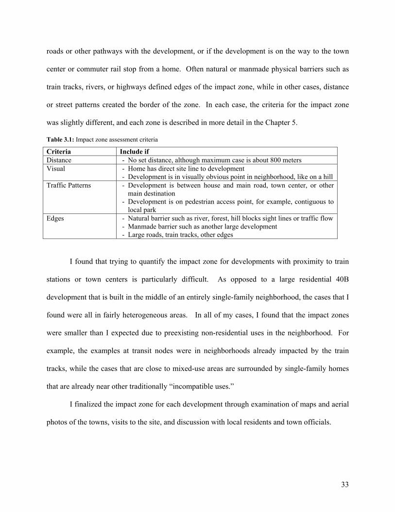
Table 3.1: Impact zone assessment criteria
Criteria Include if Distance - No set distance, although maximum case is about 800 meters Visual - Home has direct site line to development
- Development is in visually obvious point in neighborhood, like on a hill Traffic Patterns - Development is between house and main road, town center, or other
main destination - Development is on pedestrian access point, for example, contiguous to
local park Edges - Natural barrier such as river, forest, hill blocks sight lines or traffic flow
- Manmade barrier such as another large development - Large roads, train tracks, other edges
I found that trying to quantify the impact zone for developments with proximity to train
stations or town centers is particularly difficult. As opposed to a large residential 40B
development that is built in the middle of an entirely single-family neighborhood, the cases that I
found were all in fairly heterogeneous areas. In all of my cases, I found that the impact zones
were smaller than I expected due to preexisting non-residential uses in the neighborhood. For
example, the examples at transit nodes were in neighborhoods already impacted by the train
tracks, while the cases that are close to mixed-use areas are surrounded by single-family homes
that are already near other traditionally “incompatible uses.”
I finalized the impact zone for each development through examination of maps and aerial
photos of the towns, visits to the site, and discussion with local residents and town officials.
33
Quantitative Analysis
My initial task was to use sales transaction records to build a strong hedonic price model
that incorporates house characteristics and transaction dates to explain the observed sales prices.
After that, I used this model to examine the price trend of a theoretical “average house” over
time. Finally, I compared the house price index in the area impacted by the case study
development to the rest of the town in the time immediately around the completion of the project
to see what, if any, impact on prices the development had. By using a strict impact and control
area, and building a price model over time, this method allows the impact of the development to
be isolated as clearly as possible as the cause of any change in sales prices.
Data
For my analysis, I used single-family home sales transaction data collected by The
Warren Group.4 The data set includes all of the transactions in a town from 1988 through early
2005, and has information in each record such as the seller and buyer, sales price, mortgage
amount, and date of sale. The data set also contains information about the house, such as square
footage, lot size, number of bedrooms, bathrooms, fireplaces, etc. For each case study, I
analyzed all of the single-family sales transactions in the town from 1988 to the present.
The quality of the Warren Group’s data is only as good as the public record, and in some
cases, the data sets included quite a few imperfect or suspicious records. In each data set, I
found records with incomplete information, such as missing values for square footage or year
that the house was built. I eliminated all incomplete records from the analysis. In addition, the
majority of the records in the data set for Canton contained a “0” value for the number of
bedrooms. As I explain in my analysis, I decided to use the “Total Rooms” values in Canton
instead of the number of bedrooms.
34

In order to make sure that I was using as accurate a data set as possible, I endeavored to
remove suspicious data from each set before running my analyses. In each case, I excluded
records that did not seem to be legitimate arms-length transactions, for example those with sales
prices of $1 or properties that changed hands twice in one day. I also removed transactions that
had extreme values that I interpreted as outliers (for example a $57 million sales price), records
that indicated mortgage amounts higher than the sales price, and records with other suspicious
data that I investigated through The Warren Group’s full property information online database.
After an initial cleaning of the records, I ran descriptive statistics and created scatter plots to
visually represent each data set and look for outliers or other suspicious records. This
occasionally led to the elimination of other suspicious transactions, for example, lot sizes listed
as several hundred acres or huge homes on impossibly small lots. Appendix 3.1 shows the total
number of records used and eliminated for each case. In most of the data sets, the total number
of outlying or suspicious records was between 0.1 and 4.9 percent.
Hedonic Model
The process of hedonic modeling of house prices has been described in great detail in
other places, including in several papers referenced in the bibliography and in the 2004 thesis by
David Ritchay and Zoë Weinrobe. Therefore, I will limit my discussion here to a brief overview.
The theory of hedonic modeling for home prices assumes that consumers value houses as
a “bundle of goods” that includes attributes about the home itself (such as house size, lot size,
number of bedrooms, etc.) and characteristics of the neighborhood (such as real and perceived
crime rates, tax rates, and quality of the local schools). By identifying these attributes and their
contribution to the overall price, we can build a model that explains the house price (or
dependant variable) as a constant (α) added to a series of components:
35
Price = α + β1(characteristic 1) + β2(characteristic 2) + β3(characteristic 3) …
In each component, the coefficient (βx) explains the influence of that particular characteristic on
the overall price of the house. For example, if the coefficient for a characteristic like “garage” is
8%, then a house with a garage would cost 8% more than a house without a garage, assuming all
other characteristics about the house are the same.
There are two types of attributes, or variables: continuous and discrete. Continuous
variables can have any one of a range of values. For example, the interior square footage of a
house can be anything from a few hundred square feet to tens of thousands of square feet.
Discrete variables can only have a yes/no definition. For example, a house either has a pool or it
doesn’t. In order to express discrete characteristics of the houses in the model, I created a series
of dummy variables that were either turned on (a 1 value) or off (a 0 value). For example, for the
characteristic “number of bedrooms,” I could create a series of dummy variables, “1BR,” “2BR,”
“3BR,” 4+BR.” Each record would be assigned a “1” value for the appropriate dummy variable,
and “0” values for the other dummy variables. In each group of dummy variables, the lowest, or
base case is left out of the model. In my models, the base case represents the minimum scenario,
and the coefficients in the model describe the increase in price caused by the add-on represented
by the other dummy variables. For example, it is assumed that a house with no garage is the
base case, and the dummy variables of “1-car,” “2-car,” etc. can be used to describe garage
configurations. The coefficients related to these dummy variables would explain the positive (or
possibly negative) impact that different garage types has on sales prices, assuming all other
characteristics about the house are the same. Although we sometimes assume that with houses
more is more, by looking at the coefficients of the model we can quickly see the positive or
negative tradeoffs that different characteristics have on house prices.
36
In addition, some attributes, such as having a garage, might be highly valued by potential
buyers and therefore have a large impact on sales price, while others, such as the type of heat
system, might have a negligible impact. A good hedonic model includes as many of the strongly
determinative factors as possible, but does not clutter the results with factors that do not
significantly affect the price. The strength of the model is indicated by the R-squared value,
which indicates approximately what amount of the dependent variable (sales price) is being
explained by the independent variables (attributes of the house). The higher model’s R-squared
value, the better the explanatory power of the model.
In this thesis, I focus on attributes of the house and its lot. Typical neighborhood
characteristics should not be important in my model, since all of the homes are in the same town
(thus are similarly affected by local factors such as property tax rate and school quality, as well
as macroeconomic real estate trends). Thus the main factors that will determine sales prices are
the attributes of the house and lot that are available in The Warren Group data.
Sales Price Index
In order to measure the impact of the case study development on surrounding single-
family house prices, I created a house price index for both the impact area and the control (the
rest of the town). For each case study, I examined descriptive statistics about the data set to
determine the attributes of a theoretical “average house.”5 This average house differs between
the impact and control areas, as determined by the types of houses in each data set. An equation,
using coefficients derived from the hedonic model, is employed to price the theoretical average
house at the base time (1987 or 1987-88 for all of my cases). The coefficient for each non-base
sales year(s) is then added to the base year sales price to create a price index of this average
house over time. This method uses the power of the hedonic model, which explains how actual
37
prices from the data sample were affected by year of sale, to apply to the theoretical average
house as if it had sold in each year. Thus I could compare the price movement of an average
house in the impact zone to an average house elsewhere in the town from 1988 to the present.
In each town, I was particularly interested in looking at the years during and after the
permitting and construction of the case study development. Therefore, though I measured a sales
price index for the duration of the available data, it is the years around each project on which I
focus. This method assumes that news about real estate development becomes public knowledge
during the permitting process, and that the development continues to impact sales prices as it is
constructed and leased up/sold. Any impact to surrounding home prices might begin as early as
when the neighbors first heard about the development and decide to sell their home, and continue
as long as the development is seen as having an impact on the community. Though these are the
general parameters that I used, I argue that like physical impact zones, this time window differs
by the size and type of development. The specific justification for each time window is
described in the results for each case study.
1 Partial lists of 40B projects were obtained from both the Citizen’s Housing and Planning Association and from the Massachusetts Department of Housing and Community Development. Although both organizations have the responsibility to oversee units restricted by federal subsidies and monitor expiring use projects, amazingly neither seems to have a complete list of all projects permitted through the 40B process. 2 Massachusetts Projects with Subsidized Mortgages or HUD Project-Based Rental Assistance, Citizen’s Housing and Planning Association, 2004, http://www.chapa.org/expiringuse2004.pdf and Affordable Housing Online, website of apartment complexes that include subsidized units, http://www.affordablehousingonline.com/apartments.asp?mnuState=MA. 3 O’Connell, James C. Ahead or Behind the Curve?: Compact, Mixed-Use Development in Suburban Boston, August, 2004, http://www.massapa.org/pdf/report_aheadbehindcurve.pdf 4 A complete description of the data can be found on The Warren Group’s website. “About our Data,” The Warren Group, http://rers.thewarrengroup.com/sor/help/aboutourdata.asp 5 The equation for the average house includes all of the variables that were used to build the hedonic model and looks something like:
Price = constant + β1(average lot size for the sample) + β2(average interior square footage for the sample) + β3(% of houses with 2BR) + β4(% of houses with 3BR) + β5(% of houses with 4+BR) +…+ βx-1(% of houses built from 1980-1991) + βx(% of houses built after 1991)
38
CHAPTER 4: CASE STUDY PROFILES
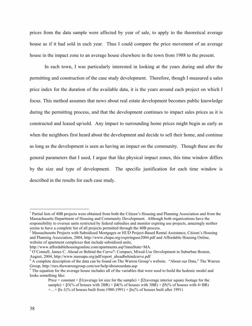
I chose five developments in towns around the Boston area as case studies. The cases
represent different strategies that towns have used to provide housing options: age- restricted
Figure 4.1: Greater Boston Area and five Case Study Towns
developments, 40B mixed-income
developments, and rezoning to
allow for more housing production.
Although no case met all of the
criteria that I initially established,
each has key characteristics. See
Appendix 4.1 for statistics about
the five towns and Appendix 4.2
for general information about the
five case study developments.
Scenario 1: Age-restricted Residential Projects
In the course of investigating potential case studies I discovered one boom area of
residential construction: age-restricted housing. Elderly developments pose little threat of
additional school children to add to the local school system and drivers to add to traffic and
parking burdens. Accordingly, towns see age-restricted housing as a relatively painless way for
them to meet their ten percent 40B requirement. Many towns are encouraging larger, mixed-
income or affordable elderly projects within their boundaries, even rezoning parts of town for
age-restricted development or cooperating with developers who want to use the comprehensive
permit process for age-restricted projects.
39

I decided to acknowledge the age-restricted housing trend by choosing two senior
developments as case studies. Both of these were completed with the cooperation of the
municipality, and to all accounts met with little objection from town residents. One (Ipswich)
used the 40B process while the other (Reading) went through the local permitting process. Both
developments are located near retail areas and relatively close to the commuter rail.
Case 1: Longwood Place at Reading
Town Profile
With a population of almost 24,000, Reading is a relatively large town. Only 12 miles
north of Boston, Reading lies on both Interstate 93 and 95 and has an MBTA commuter rail
station. Reading is undergoing changes, with two large residential and mixed-use developments
under construction in the area adjacent to the commuter rail station. However, these projects
have come to Reading through the 40B process, and it is only now that the town is
acknowledging its potential for transit-oriented development.
Reading’s residential zoning primarily requires single-family development on minimum
lot sizes from 15,000 square feet to an acre. The current zoning ordinance does incorporate
inclusionary requirements in its municipal reuse district and its planned unit development (PUD)
and planned residential development (PRD) bylaws.1 In one particularly Machiavellian section
of the PRD bylaw, the zoning requires at least ten percent of the units are affordable, 15% if the
site is within 300 feet of the town line. Currently, Reading has about 7.9% of its units counted as
affordable, and is about 450 units short of the ten percent 40B requirement.
40
Planning Efforts
Reading’s new Community Development Plan begins with the objective: “Preserve the
architectural heritage and the traditional village character of the Town” and follows with an
ominous first goal: “Preserve the Town as a primarily single-family, owner-occupied residential
community.2” However, the recent approval of several 40B projects comprising over 500 units
throughout Reading has forced the town to undertake proactive housing planning. The new
Community Development plan includes a list of housing initiatives from adopting inclusionary
zoning to reforming a housing committee, to hiring a housing staff person. The plan also
includes a specific proposal to rezone downtown districts for mixed-use development. However,
the town’s lack of staff and financial resources make concrete progress difficult. According to a
member of the planning staff, the town has been in the position of reacting to 40B developments
instead of having the ability to control the development process from the outset.
Development Profile
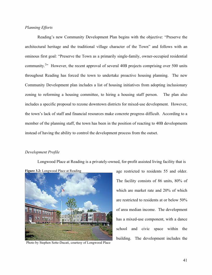
Longwood Place at Reading is a privately-owned, for-profit assisted living facility that is
Figure 3.2: Longwood Place at Reading
Photo by Stephen Sette-Ducati, courtesy of Longwood Place
age restricted to residents 55 and older.
The facility consists of 86 units, 80% of
which are market rate and 20% of which
are restricted to residents at or below 50%
of area median income. The development
has a mixed-use component, with a dance
school and civic space within the
building. The development includes the
41
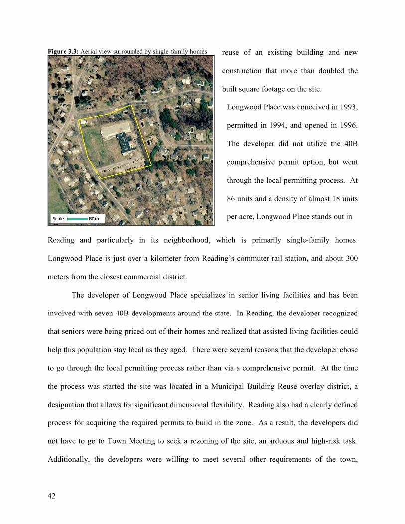
Figure 3.3: Aerial view surrounded by single-family homes
reuse of an existing building and new
construction that more than doubled the
built square footage on the site.
Longwood Place was conceived in 1993,
permitted in 1994, and opened in 1996.
The developer did not utilize the 40B
comprehensive permit option, but went
through the local permitting process. At
86 units and a density of almost 18 units
per acre, Longwood Place stands out in
Reading and particularly in its neighborhood, which is primarily single-family homes.
Longwood Place is just over a kilometer from Reading’s commuter rail station, and about 300
meters from the closest commercial district.
The developer of Longwood Place specializes in senior living facilities and has been
involved with seven 40B developments around the state. In Reading, the developer recognized
that seniors were being priced out of their homes and realized that assisted living facilities could
help this population stay local as they aged. There were several reasons that the developer chose
to go through the local permitting process rather than via a comprehensive permit. At the time
the process was started the site was located in a Municipal Building Reuse overlay district, a
designation that allows for significant dimensional flexibility. Reading also had a clearly defined
process for acquiring the required permits to build in the zone. As a result, the developers did
not have to go to Town Meeting to seek a rezoning of the site, an arduous and high-risk task.
Additionally, the developers were willing to meet several other requirements of the town,
42
including surpassing the inclusionary zoning requirement of the Municipal Building Reuse
district,3 retaining a commercial tenant (the dance school) on site, and incorporating civic uses
both within the building and on the property.
The developers did require three variances for the project: a reduction of minimum
parking spaces, relief from side-yard setback requirements, and an exception to the requirements
regarding overall building size and massing.4 Two of these permits were appealed: the side yard
variance by an abutter and the special permit by the Reading Housing Authority. The developers
negotiated with the abutter and changed the design of the building slightly, whereupon the appeal
was dropped. The Reading Housing Authority appealed over the supervision of the affordable
units, a responsibility they believed the zoning bylaws designated to them. The situation was
resolved when the Housing Authority, the Board of Selectmen, and the developer signed a three-
way agreement requiring the owners of Longwood Place to certify that at least half of the
affordable units would be rented to residents with Reading ties in perpetuity.
Although the Reading permitting process was straightforward, the developer wonders if
Longwood Place would have been smoother as a 40B project. However, the developer
remembers that the Reading Board of Selectmen made it clear that they strongly preferred that
the project go through town channels. As a result, 40B helped the process because both the
developer and the town knew that it could be used if necessary, and both parties were
encouraged to support and move Longwood Place forward.
43
Case 2: Oak Hill
Town Profile
Ipswich is a small rural town of about 12,000 people on the North Shore of
Massachusetts about 28 miles northeast of Boston. It is known for its extensive protected open
space and its large, well-preserved collection of historic homes.5 The town has a compact center
with an MBTA commuter rail stop. Originally a working mill town, Ipswich became a summer
retreat for families from Boston and its environs. Today, Ipswich is primarily a bedroom
community to Boston. In the 2000 census, the median household income of Ipswich was
$57,284, slightly lower than the Boston metropolitan area median. Although not particularly
affluent, household incomes have increased considerably in Ipswich over the last decade,
indicating that the wealthy population is growing in the town. Simultaneously, the demographics
of Ipswich have shifted, with middle-aged families replacing young adults and the elderly.6
These trends might in part be explained by the town’s booming real estate market. In the last
decade, the sales price of the median single-family home in Ipswich increased by 175%.7 In
addition, many homes that were being used as second or vacation homes have changed to
primary residences, indicating Ipswich’s growing popularity as a place to call home.
Construction trends in town have favored the single-family home, with the number of
single-family units growing between 1990 and 2000. As elsewhere in Massachusetts, houses are
getting larger in Ipswich, and new eight and nine-room homes are common. Meanwhile, the
number of multifamily structures (with three or more units) fell as a percent of total housing
units in Ipswich over the same decade. The construction of rental housing has been particularly
sluggish. In fact, the town had fewer rental units in 2000 than it did in 1990.8 As of early 2005,
44
7.8% of the town’s housing units were considered affordable, just over 100 units short of the 40B
ten percent goal.9 According to CHAPA, this number changed by less than 1% since 1997.10
Ipswich’s zoning reflects its rural nature. Approximately 93% of the land in Ipswich is
designated as one of three “Rural Residential Zones” (RRZ), which have a minimum lot size of
two acres. These zones allow single-family homes by right and two-family homes by special
permit. Around the town center, approximately 2.2% of the town’s land is zoned as “Intown
Residential” (IR), where single- and two-family homes are allowed by right, multifamily is
allowed by special permit, and minimum lot sizes are 10,000 square feet and up.11 The town’s
recent efforts to promote housing development have focused on this IR district.
Planning Efforts
Ipswich’s zoning bylaw and its housing plan are oriented toward protecting open space
and preserving the rural character of the town, but planning officials maintain that the town is
committed to increasing the production of affordable housing. Ipswich has recently taken
several steps to encourage housing starts. The 2003 Housing Action Plan outlines four policy
areas and thirteen distinct actions to move Ipswich closer to the ten percent goal. The plan
suggests creating a new Village Incentive District (VI), to encourage higher densities in
developed areas and to take advantage of existing infrastructure. Under this proposal, up to four-
unit residential buildings could be built in the VI district on smaller lots than currently allowed in
the zoning ordinance. The plan suggests using a transfer of development rights to increase
allowable densities in this district while preserving undeveloped land in rural districts.
Although many of the proposals in the plan, including the VI district, have yet to be
passed, Ipswich has been able to take a few concrete actions. For example, zoning has twice
45
been amended (in 1999 and in 2001) to allow for the creation of small accessory units in
preexisting residential buildings or in secondary structures on residential lots. In 2003, Town
Meeting passed an amendment to the zoning bylaw that allows infill development of housing on
non-conforming (too small) lots in the Intown Residence district. The town has also enacted an
inclusionary zoning provision that grants developers density bonuses by special permit if they
make a minimum of ten percent of the units affordable (to households at 70% of area median
income). Planning staff explain that the provision is intended to encourage more projects to go
through the local process instead of the comprehensive permit alternative, and notes that three
projects have been approved in the year and a half since the provision was enacted.
The town has participated in three recent comprehensive permit projects that are
described as amicable and that were done with the cooperation of the town and minimal
opposition from abutters and residents.
Development Profile
Oak Hill is a 33-unit rental housing development that is 100% affordable to residents at
up to 80% of area median income. It was built as congregate housing and is age-restricted to
elderly members of the community. The project was developed by the Immanuel Baptist
Church, which donated the land and raised the majority of the money for development. The
development is situated in the heart of downtown Ipswich, on one of the main commercial
streets, less than a half a mile from the MBTA commuter rail station. One member of Immanuel
involved with the development of Oak Hill remembers that the needs of the elderly residents
were a critical factor in situating the project. While seniors were less likely to utilize proximity
46
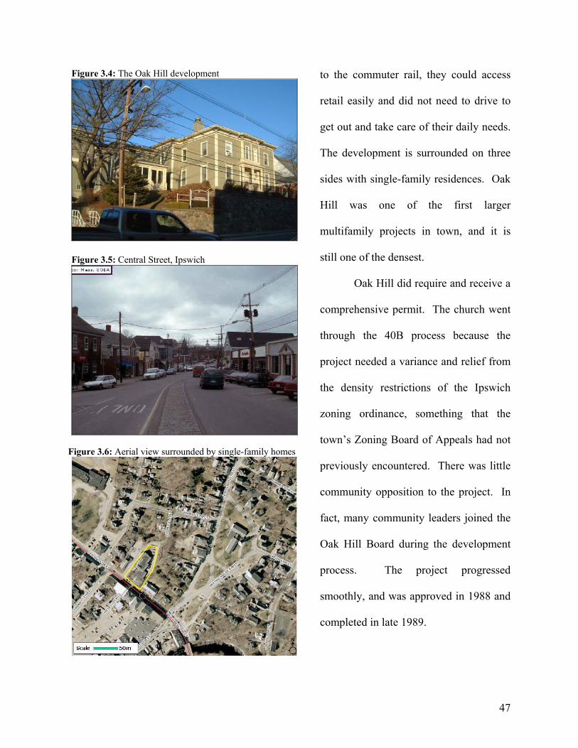
Figure 3.4: The Oak Hill development
Figure 3.5: Central Street, Ipswich
Figure 3.6: Aerial view surrounded by single-family homes
to the commuter rail, they could access
retail easily and did not need to drive to
get out and take care of their daily needs.
The development is surrounded on three
sides with single-family residences. Oak
Hill was one of the first larger
multifamily projects in town, and it is
still one of the densest.
Oak Hill did require and receive a
comprehensive permit. The church went
through the 40B process because the
project needed a variance and relief from
the density restrictions of the Ipswich
zoning ordinance, something that the
town’s Zoning Board of Appeals had not
previously encountered. There was little
community opposition to the project. In
fact, many community leaders joined the
Oak Hill Board during the development
process. The project progressed
smoothly, and was approved in 1988 and
completed in late 1989.
47
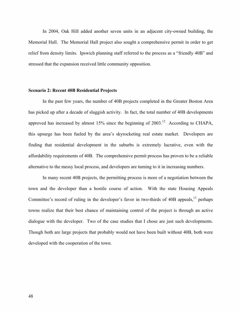
In 2004, Oak Hill added another seven units in an adjacent city-owned building, the
Memorial Hall. The Memorial Hall project also sought a comprehensive permit in order to get
relief from density limits. Ipswich planning staff referred to the process as a “friendly 40B” and
stressed that the expansion received little community opposition.
Scenario 2: Recent 40B Residential Projects
In the past few years, the number of 40B projects completed in the Greater Boston Area
has picked up after a decade of sluggish activity. In fact, the total number of 40B developments
approved has increased by almost 15% since the beginning of 2003.12 According to CHAPA,
this upsurge has been fueled by the area’s skyrocketing real estate market. Developers are
finding that residential development in the suburbs is extremely lucrative, even with the
affordability requirements of 40B. The comprehensive permit process has proven to be a reliable
alternative to the messy local process, and developers are turning to it in increasing numbers.
In many recent 40B projects, the permitting process is more of a negotiation between the
town and the developer than a hostile course of action. With the state Housing Appeals
Committee’s record of ruling in the developer’s favor in two-thirds of 40B appeals,13 perhaps
towns realize that their best chance of maintaining control of the project is through an active
dialogue with the developer. Two of the case studies that I chose are just such developments.
Though both are large projects that probably would not have been built without 40B, both were
developed with the cooperation of the town.
48
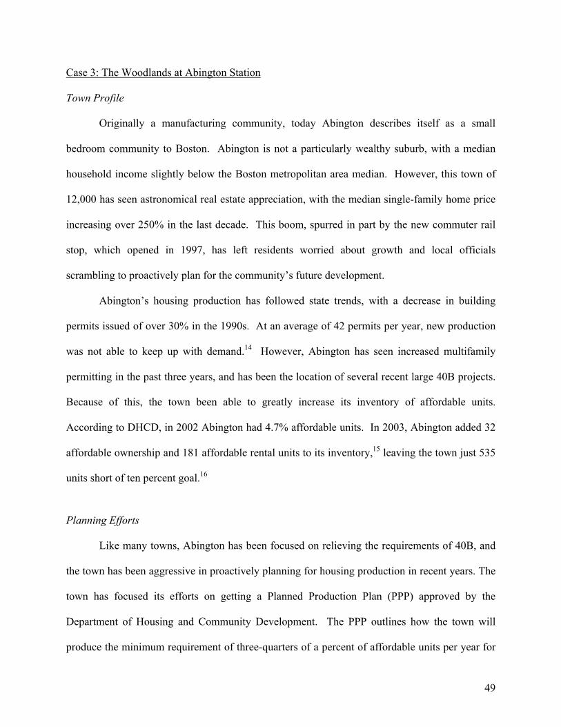
Case 3: The Woodlands at Abington Station
Town Profile
Originally a manufacturing community, today Abington describes itself as a small
bedroom community to Boston. Abington is not a particularly wealthy suburb, with a median
household income slightly below the Boston metropolitan area median. However, this town of
12,000 has seen astronomical real estate appreciation, with the median single-family home price
increasing over 250% in the last decade. This boom, spurred in part by the new commuter rail
stop, which opened in 1997, has left residents worried about growth and local officials
scrambling to proactively plan for the community’s future development.
Abington’s housing production has followed state trends, with a decrease in building
permits issued of over 30% in the 1990s. At an average of 42 permits per year, new production
was not able to keep up with demand.14 However, Abington has seen increased multifamily
permitting in the past three years, and has been the location of several recent large 40B projects.
Because of this, the town been able to greatly increase its inventory of affordable units.
According to DHCD, in 2002 Abington had 4.7% affordable units. In 2003, Abington added 32
affordable ownership and 181 affordable rental units to its inventory,15 leaving the town just 535
units short of ten percent goal.16
Planning Efforts
Like many towns, Abington has been focused on relieving the requirements of 40B, and
the town has been aggressive in proactively planning for housing production in recent years. The
town has focused its efforts on getting a Planned Production Plan (PPP) approved by the
Department of Housing and Community Development. The PPP outlines how the town will
produce the minimum requirement of three-quarters of a percent of affordable units per year for
49
the next five years. As of 2005, Abington is one of only 29 towns that has a PPP approved by the
DHCD. The plan counts two 40B projects, including The Woodlands, as contributing to its
annual addition of affordable units. At 40 units per year, the 192 units at The Woodlands alone
nearly achieves Abington’s 0.75% goal.
Abington has also been proactive in its outlook for future development, and the town has
been repeatedly recognized for its approach to growth. In 2003, Abington Town Meeting voted
to rezone two areas to encourage multi-family residential development. The first, the Central
Business District (CBD), allows for both the creation of accessory units and higher-density
multifamily structures. The second, the Transit Oriented Development (TOD) Zone, won the
Governor’s Smart Growth Leadership Award in December of 2004.17 The district, which
comprises 30 acres around the commuter rail station, encourages mixed-use development and
incorporates features such as reduced parking ratios and required pedestrian connections to the
train station. In a 2004 audit, Abington was recognized by the Massachusetts Vision 2020 as one
of only three communities out of the 42 studied that are currently “growing smartly.18”
According to Abington planning staff, The Woodlands development was the impetus for
the rezoning proposals. The town wanted to be able to control the rate and form of development
in these areas, and the rezoning was an attempt to do that. While the original intent of the TOD
district was to encourage business development around the train station, planning staff points to
The Woodlands as an example of the success of dense residential development in that area.
Development Profile
The Woodlands at Abington Station is a 192-unit rental property developed by Beacon
Residential Properties. The project was permitted through the comprehensive permit process and
50
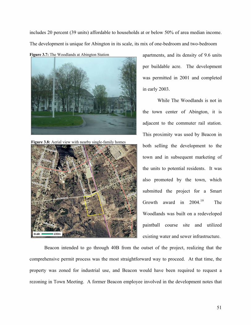
includes 20 percent (39 units) affordable to households at or below 50% of area median income.
The development is unique for Abington in its scale, its mix of one-bedroom and two-bedroom
Figure 3.7: The Woodlands at Abington Station
Figure 3.8: Aerial view with nearby single-family homes
apartments, and its density of 9.6 units
per buildable acre. The development
was permitted in 2001 and completed
in early 2003.
While The Woodlands is not in
the town center of Abington, it is
adjacent to the commuter rail station.
This proximity was used by Beacon in
both selling the development to the
town and in subsequent marketing of
the units to potential residents. It was
also promoted by the town, which
submitted the project for a Smart
Growth award in 2004.19 The
Woodlands was built on a redeveloped
paintball course site and utilized
existing water and sewer infrastructure.
Beacon intended to go through 40B from the outset of the project, realizing that the
comprehensive permit process was the most straightforward way to proceed. At that time, the
property was zoned for industrial use, and Beacon would have been required to request a
rezoning in Town Meeting. A former Beacon employee involved in the development notes that
51

it would have been very difficult getting public support for a residential project of that size and
adds that going to Town Meeting for the rezoning would have been an extremely expensive and
high-risk process.
Abington worked with Beacon throughout the project, trying to negotiate the best deal
possible for the town while ensuring that the permitting process moved forward. The town was
particularly motivated to ensure the permit approval for The Woodlands because the 192 rental
units would get Abington to the ten percent 40B requirement. Although the scale and tenure of
the project and its traffic impacts were of some concern to the neighbors, as was water supply
and sewage capacity, public resistance to the project was never very great. This was in part
because the residential development was an improvement over the former industrial use.
Overall, The Woodlands permitting process was non-adversarial and successful largely due to
the negotiation between the developer and the town. The former Beacon employee concluded
that without 40B, they wouldn’t have had a chance of getting a development of that size
approved in Abington, or in any other town in the area.
Case 4: Fairhaven Garden
Town Profile
One of the wealthiest and most expensive towns in the Greater Boston Area, Concord had
a 2004 average single-family home value of $898,455.20 At almost $100,000, the town’s median
household income is 167% of the Greater Boston Area’s.
Concord suffers from the anti-development trend that is facing towns in the region.
Construction of new homes is almost non-existent in the town. In the past ten years, Concord
has granted just 306 residential building permits, with only two of these (both 40B projects) for
52
multifamily structures.21 Even the trickle of new single-family permits cannot truly be
considered new construction, since an average of two-thirds of the single-family permits every
year are for teardowns.22 In practice, teardowns are used to replace smaller homes with large new
houses, often combining lots (and thus reducing overall density) in the process. Concord’s
housing stock reflects this trend, with the average size of a new house increasing from 3,123
square feet in 1980 to 8,995 square feet in 2000.23
Over half of Concord’s land is designated as preserved open space, and the town’s
remaining developable land is almost entirely zoned for single-family homes with one- or two-
acre minimum lot sizes. Ironically, much of Concord’s appeal is its traditional New England
town feel, with businesses and residences crowded around the town common, a typology that is
found around the West Concord town center. However, this traditional form is impossible to
recreate under Concord’s current zoning and building trends.
As of August of 2004, Concord had only reached 4.92% affordable units, far short of the
40B ten percent requirement and the lowest of any of the case study towns.24 The town has seen
only four developments with an affordability component since 2000. Two were small (a total of
17 homes) single-family home ownership projects undertaken by the Concord Housing Trust and
a non-profit developer, and two were 40B rental projects.25 The town submitted a Planned
Production plan to the DHCD in 2004 and is waiting for it to be approved.
Planning Efforts
A review of Concord’s pertinent planning documents indicates that affordable housing is
not a high priority for the town. While affordable housing is mentioned repeatedly in Concord’s
zoning bylaws, there is no specific requirement or incentive for developers to incorporate an
53
affordability component. The town’s 2004 Affordable Housing Fact sheet points out (perhaps
ironically?26) that Concord is “somewhat unique” in including households with up to 150% of
the area median income (currently almost $125,000 for a family of four) in its affordable housing
designation. In fact, the town’s zoning includes two levels of affordability, “starter units,” for
households up to 110% of area median income, and “moderately priced units,” for households up
to 150%.27 Both the Planned Residential Bylaw and the Residential Cluster Development
sections of the town’s zoning ordinance28 allow a density bonus for developments that include
units at or below these affordability levels. However, in both cases, the bonus is undefined and
is granted at the discretion of the Planning Board.
In 1992, Concord passed an Inclusionary Housing Bylaw that requires all large
subdivisions to set aside land for the construction of affordable units or to donate funds for the
offsite production of affordable units. This has not proven to be efficacious in actually getting
units constructed, as the market rate for units is so high in the area that developers can easily
contribute the cash equivalent and avoid incorporating affordability into their project. An
example of this is Concord Crossing, a new mixed-use redevelopment of an industrial site across
from the Concord Center commuter rail station. The project includes 20 rental units, and was
granted a special permit and density variance. Although the developer initially planned to
include two affordable units in the project, he decided to take the offsite payment option instead
after realizing that market rents were very high.
There is no required inclusionary zoning in Concord, but town planners list efforts to
promote affordable housing development including asking developers to include an affordability
component and working with developers on proposed 40B projects. Concord is not considering
adopting the new Smart Growth overlay district of Chapter 40R because it requires too much
54
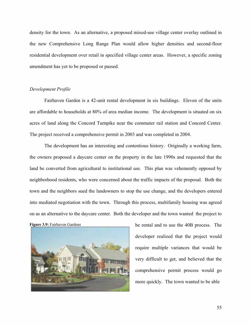
density for the town. As an alternative, a proposed mixed-use village center overlay outlined in
the new Comprehensive Long Range Plan would allow higher densities and second-floor
residential development over retail in specified village center areas. However, a specific zoning
amendment has yet to be proposed or passed.
Development Profile
Fairhaven Garden is a 42-unit rental development in six buildings. Eleven of the units
are affordable to households at 80% of area median income. The development is situated on six
acres of land along the Concord Turnpike near the commuter rail station and Concord Center.
The project received a comprehensive permit in 2003 and was completed in 2004.
The development has an interesting and contentious history. Originally a working farm,
the owners proposed a daycare center on the property in the late 1990s and requested that the
land be converted from agricultural to institutional use. This plan was vehemently opposed by
neighborhood residents, who were concerned about the traffic impacts of the proposal. Both the
town and the neighbors sued the landowners to stop the use change, and the developers entered
into mediated negotiation with the town. Through this process, multifamily housing was agreed
on as an alternative to the daycare center. Both the developer and the town wanted the project to
Figure 3.9: Fairhaven Gardens
be rental and to use the 40B process. The
developer realized that the project would
require multiple variances that would be
very difficult to get, and believed that the
comprehensive permit process would go
more quickly. The town wanted to be able
55
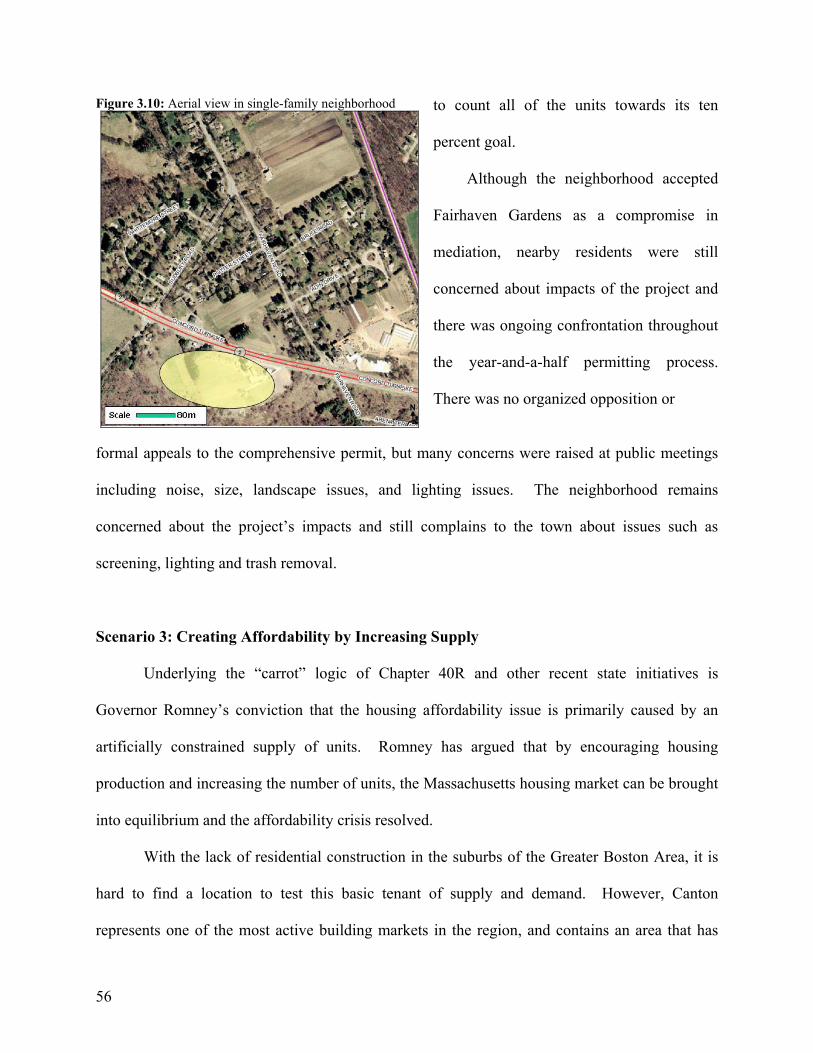
Figure 3.10: Aerial view in single-family neighborhood to count all of the units towards its ten
percent goal.
Although the neighborhood accepted
Fairhaven Gardens as a compromise in
mediation, nearby residents were still
concerned about impacts of the project and
there was ongoing confrontation throughout
the year-and-a-half permitting process.
There was no organized opposition or
formal appeals to the comprehensive permit, but many concerns were raised at public meetings
including noise, size, landscape issues, and lighting issues. The neighborhood remains
concerned about the project’s impacts and still complains to the town about issues such as
screening, lighting and trash removal.
Scenario 3: Creating Affordability by Increasing Supply
Underlying the “carrot” logic of Chapter 40R and other recent state initiatives is
Governor Romney’s conviction that the housing affordability issue is primarily caused by an
artificially constrained supply of units. Romney has argued that by encouraging housing
production and increasing the number of units, the Massachusetts housing market can be brought
into equilibrium and the affordability crisis resolved.
With the lack of residential construction in the suburbs of the Greater Boston Area, it is
hard to find a location to test this basic tenant of supply and demand. However, Canton
represents one of the most active building markets in the region, and contains an area that has
56
recently added a significant number of units and been revitalized as a mixed-use, transit oriented
town center. Even though the new developments in Canton Center were not built with a specific
affordability component, I chose to include the town as a case study because of the scope of the
transformation of the area and the large number of new residential developments built in the last
five years.
Case 5: Canton Center
Town Profile
The town of Canton lies 18 miles southwest of Boston. Though the town is primarily
residential, several parts of Canton, including the area around the Canton Center commuter rail
station, have a mix of residential, commercial, and industrial uses. Canton’s current zoning
includes many types of residential areas, and has several inclusionary zoning provisions with
affordability requirements from five to fifteen percent. As of 2005, Canton is the only town of
the five case studies that has reached the ten percent 40B requirement.
Planning efforts
With a central commuter rail stop, a mixed-use main street, and a number of large,
relatively dense residential projects, Canton Center is an example of many of the principles of
Smart Growth development. However, a local developer recalls that in the late 1990s, Canton
Center was a disaster, with dilapidated buildings, run-down retail, and many abandoned or
underutilized parcels. The turning point for Canton Center was the establishment of the Canton
Center Economic Opportunity District (CCEOD) in 2000. At the time the economic
revitalization of the area was one of the primary goals of the planning department. The CCEOD
57

zoning bylaw was the result of a two-year public process in which the town and consultants from
the Metropolitan Area Planning Council gathered ideas and requirements from town officials,
residents, and local businesses, created the bylaw, and built support for the rezoning. Many
people were nervous about the rezoning and central points of contention included density, the
spread of commercial uses, and the concern that Canton still look like a town and not become a
city. In response, the boundaries of the CCEOD zone were reduced to keep the higher-density
zone to the downtown area and restrict commercial uses to Washington Street and design
guidelines were included in the bylaw to reflect the style of the traditional New England town
center. Local planners spent two years in meetings and charrettes, and were able to get
widespread support for the amendment. In 2000, the CCEOD bylaw passed Town Meeting by a
unanimous vote.
The overlay district encourages mixed-use development with relatively flexible density
and dimensional requirements. Although the CCEOD District was not conceived as a way to
increase the production of affordable housing, in 2004, an inclusionary zoning provision was
added to the CCEOD overlay zone.29 This amendment requires a minimum of 15 percent of
affordable units be included in residential projects in the overlay area. When the CCEOD was
passed, the town was unwilling to commit any public funds to the revitalization effort and town
planners were not certain that the new district could attract private money to Canton Center. As
projects in the zone have proven economically successful and the residential real estate market
has appreciated, the town decided to require an affordable component for new developments.
The new provision has not slowed development in the area, and several new projects with an
affordability component are currently under construction.
58
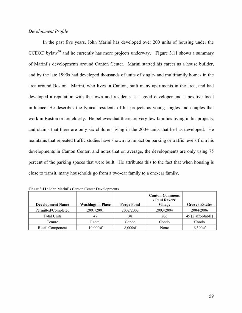
Development Profile
In the past five years, John Marini has developed over 200 units of housing under the
CCEOD bylaw30 and he currently has more projects underway. Figure 3.11 shows a summary
of Marini’s developments around Canton Center. Marini started his career as a house builder,
and by the late 1990s had developed thousands of units of single- and multifamily homes in the
area around Boston. Marini, who lives in Canton, built many apartments in the area, and had
developed a reputation with the town and residents as a good developer and a positive local
influence. He describes the typical residents of his projects as young singles and couples that
work in Boston or are elderly. He believes that there are very few families living in his projects,
and claims that there are only six children living in the 200+ units that he has developed. He
maintains that repeated traffic studies have shown no impact on parking or traffic levels from his
developments in Canton Center, and notes that on average, the developments are only using 75
percent of the parking spaces that were built. He attributes this to the fact that when housing is
close to transit, many households go from a two-car family to a one-car family.
Chart 3.11: John Marini’s Canton Center Developments
Development Name Washington Place Forge Pond
Canton Commons / Paul Revere
Village Grover Estates Permitted/Completed 2001/2001 2002/2003 2003/2004 2004/2006
Total Units 47 38 206 45 (2 affordable) Tenure Rental Condo Condo Condo
Retail Component 10,000sf 8,000sf None 6,500sf
59
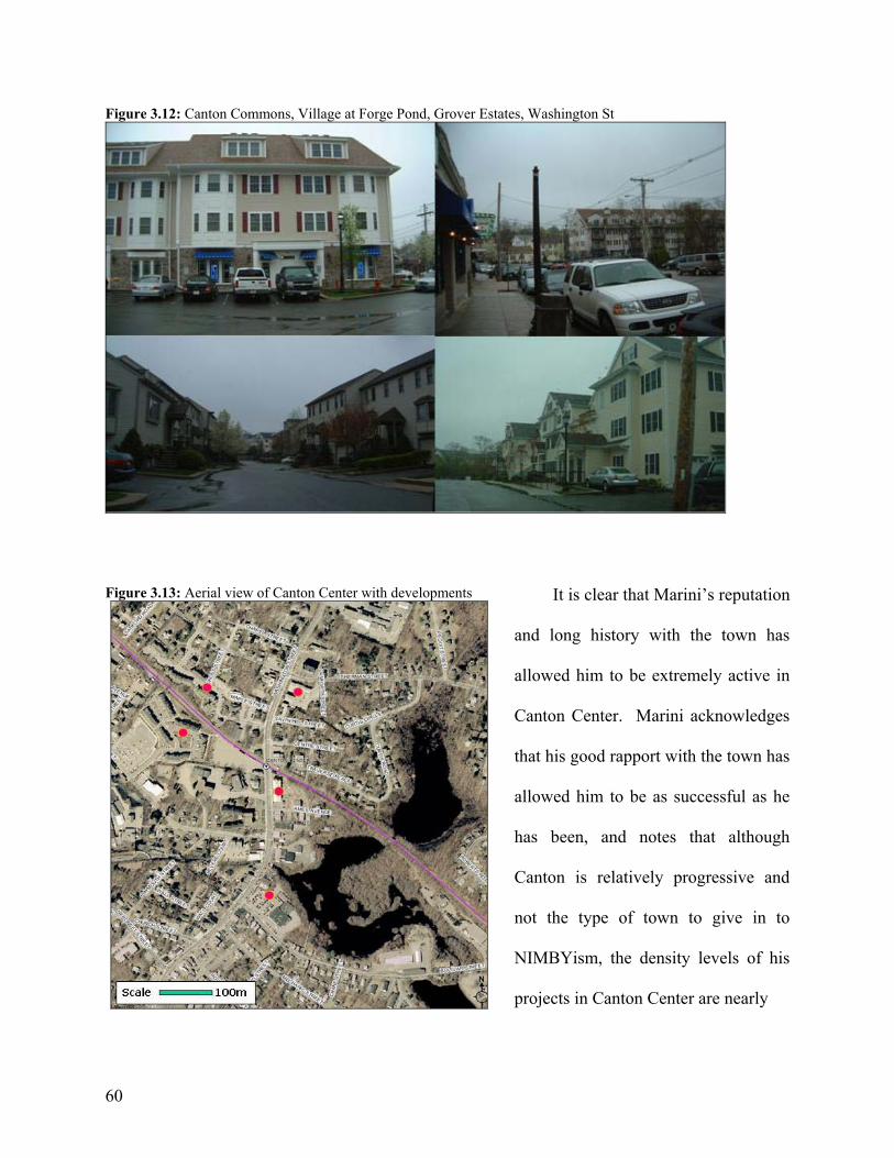
Figure 3.12: Canton Commons, Village at Forge Pond, Grover Estates, Washington St
Figure 3.13: Aerial view of Canton Center with developments It is clear that Marini’s reputation
and long history with the town has
allowed him to be extremely active in
Canton Center. Marini acknowledges
that his good rapport with the town has
allowed him to be as successful as he
has been, and notes that although
Canton is relatively progressive and
not the type of town to give in to
NIMBYism, the density levels of his
projects in Canton Center are nearly
60
impossible to achieve in any town. Though Marini chose to avoid public subsidies and develop
within the conventional market, he also acknowledges that if it wasn’t for 40B, there wouldn’t be
any multifamily built anywhere in Massachusetts. Marini, who once served on the Board of
Directors of the Massachusetts Housing Finance Authority, believes that affordable housing will
come without anyone trying and that the building of apartments in Massachusetts will eventually
result in a softening of the market.
1 Reading’s PUD bylaw allows for a height bonus if at least ten percent of the units are affordable at below 80% AMI, and the PRD bylaw includes a density bonus (for PRD-G) or a requirement (for PRD-M) for at least ten percent of affordable units (100% of AMI) or 15% moderately priced units (at 125% AMI). Zoning By-laws, Town of Reading Zoning Board of Appeals, http://www.ci.reading.ma.us/planning/zbahomepage.htm, 2 Reading Community Development Plan, Reading Master Plan Advisory Committee, http://www.ci.reading.ma.us/planning/finalmapcplan.pdf 3 The zoning requires a minimum of ten percent of units be set aside for “very-low-income, low-income and moderate-income families and/or elderly households.” Zoning By-laws, Town of Reading Zoning Board of Appeals, http://www.ci.reading.ma.us/planning/zbahomepage.htm, p. 29 4 Longwood Place, like many assisted living facilities, is one large connected structure, allowing senior residents to move around the facility in a protected environment. 5 And for fried clams – try The Clam Box! 6 Ipswich Demographic Changes, Chuck Koller’s Homepage, http://www.ckollars.org/demographicchanges.html 7 From The Warren Group’s Town Stats (http://rers.thewarrengroup.com/townstats/ts_login.asp). The median single-family home price was $165,500 in 1994 and $455,000 in 2004. 8 Ipswich Housing Action Plan, p.1 SOURCE 9 “Not Even the YMCA is Safe from Community Opposition,” The NIMBY Report, National Low Income Housing Coalition, October, 2004, http://www.nlihc.org/nimby/102004.htm 10 Analysis of the 2005 Subsidized Housing Inventory, Citizens’ Housing and Planning Association, 2005, http://www.chapa.org/0540banalysis.pdf 11 Ipswich Housing Action Plan. From the Community Development Plan, Town of Ipswich, 2003, http://www.town.ipswich.ma.us/plandev/pdf/development%20plan/ICDP.htm 12 40B Housing Units Built and Proposed, CHAPA, 2005 13 Chapter 40B Fact Sheet, CHAPA, http://www.chapa.org/40b_fact.html 14 Regional Policy Plan, Old Colony Regional Planning Council, 1999, http://www.ocpcrpa.org/OCPC%20Reg-Policy-Plan%202000.pdf 15 Department of Housing and Community Development, Executive Order 418 Housing Certification: Abington, August, 2004, https://www2.massdhcd.com/e418portal/FY05/CommReport02.asp?MNO=1&FY=2005 16 Abington Affordable Housing Strategy, September, 2003, http://www.mass.gov/dhcd/ToolKit/PProd/apAbing.pdf 17 Local Heroes and Super Models: Governor’s Awards for Smart Growth Leadership, Massachusetts Office of Commonwealth Development, Dec 2004, http://www.mass.gov/ocd/docs/smart/sgacs.pdf 18 Smart Growth Audit, Vision 2020, July 2004, http://www.srpedd.org/smartgrowthaudit/smartgrowthaudit.pdf 19 Crane conversation, May 2005. 20 According to the Town of Concord Assessor’s Office 21 General Obligation Bond Summary Statement, Town of Concord, February, 2005, http://www.concordnet.org/finance/OS022305.pdf 22 2004 Concord Annual Town Report, Department of Planning and Land Management, Town of Concord, http://www.concordnet.org/townmgr/2004%20Town%20Report/0408_cd/dplm/nrc.html
61
23 Chapter 3 – Housing, Comprehensive Long Range Plan, Comprehensive Long Range Plan Committee, May 2003, http://www.concordvision.org/PDF/Chapter_3.pdf 24 2004 Concord Annual Town Report, Town of Concord, Department of Planning and Land Management, 2004, http://www.concordnet.org/townmgr/2004%20Town%20Report/0408_cd/dplm/tpd.html 25 The 40B projects include the case study development, Fairhaven Garden, and Warner Woods, an 80 unit mixed-income rental project scheduled to be completed in 2006. 26 The fact sheet goes on to point out that only one employee of the town of Concord (the Finance Director) qualifies as even the median income, and that no employee of the town makes the 150% or even the 110% “starter income” set in the bylaw. Affordable Housing Fact Sheet, Town of Concord, 2004, http://www.concordnet.org/dplm/Affordability%20Fact%20Sheet.pdf 27 Zoning Bylaw, Town of Concord, http://www.concordnet.org/dplm/2004%20Zoning%20Bylaw.pdf 28 Sections 9 and 10, Zoning Bylaw, Town of Concord, http://www.concordnet.org/dplm/2004%20Zoning%20Bylaw.pdf 29 Section 5.66.11, Zoning Bylaw, Town of Canton, http://www.town.canton.ma.us/PDF_files/Zoning-Bylaw.pdf 30 Zoning Bylaw, Town of Canton, http://www.town.canton.ma.us/PDF_files/Zoning-Bylaw.pdf
62
CHAPTER 5: QUANTITATIVE ANALYSIS
This chapter details the results of the analysis of house prices in each of the five case
studies. For each case study, I used descriptive statistics and regression analysis to build hedonic
models that explain the observed house sale prices for both the control and impact data sets. I
also build the sales price index for the average home through time using the equation that was
constructed with the coefficients from the hedonic model. I then compare the price trend in the
impact zone to the rest of the town, paying particular attention to the years during and
immediately following permitting and construction of the development. Because the
independent variables used to build the model1 were identical in the control and impact zones
and both data sets represent homes in the same town (minimizing the impact of difference in
macro-level externalities such as school district and tax rate), differences between the two can be
attributed to the introduction of a large new development.
Although each case is slightly different, in general, I compared sales in the years directly
before permitting of the development with those in the years directly after the construction and
lease-up of the development was concluded. This method assumes that potential negative
impacts from a development begin when the project is considered likely to be built (for example,
has final approvals in the form of a comprehensive or other permit) and peaks after the
construction is finished and occupancy is stabilized. It assumes that the market will react to any
negative externalities of the development within that timeframe.
There are arguments that multifamily and mixed-income developments age poorly, become
run down and increasingly impact the neighborhood, but the duration of that kind of analysis is
outside the scope of this study. However, for some of the older case studies, it is possible to
63

compare the impact and control areas for many years after the development was constructed and
see if there is any ongoing or continuing impact on sales prices.
In every case but Abington, I use paired years for the sales period variable to ensure that
there were multiple observations for each period. A small sample size increases noise in the
results, and incorporating more observations reduces standard error and provides a more accurate
estimate of the impact of each sales period on the sales price. Further differences in variables are
described in each case below. Details about the variables I used to construct the regression
analysis can be reviewed in Appendix 5.1.
Case 1: Longwood Place at Reading
Location and Impact Zone
Longwood Place is a large age-restricted development situated on an expansive parcel in
the middle of a single family neighborhood. There are single-family homes to the east, south,
and west, and a forest forms a natural barrier to the northeast. Main Street, the nearest
commercial street, is two blocks to the west. This street creates another edge of the impact zone.
Longwood Place is very large and its open campus is visible throughout the surrounding
neighborhood. In addition, Longwood Place borders Charles Street, a main feeder street from
the neighborhood to the north to Main Street.
The impact area for this case comprises about nine streets of homes, and includes single-
family homes as far as 500 meters or three streets away from the development. Houses with a
direct visual line to the development were included in the impact zone.
64
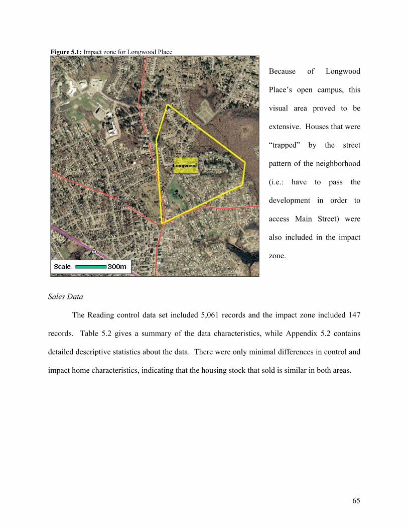
Figure 5.1: Impact zone for Longwood Place
Because of Longwood
Place’s open campus, this
visual area proved to be
extensive. Houses that were
“trapped” by the street
pattern of the neighborhood
(i.e.: have to pass the
development in order to
access Main Street) were
also included in the impact
zone.
Sales Data
The Reading control data set included 5,061 records and the impact zone included 147
records. Table 5.2 gives a summary of the data characteristics, while Appendix 5.2 contains
detailed descriptive statistics about the data. There were only minimal differences in control and
impact home characteristics, indicating that the housing stock that sold is similar in both areas.
65
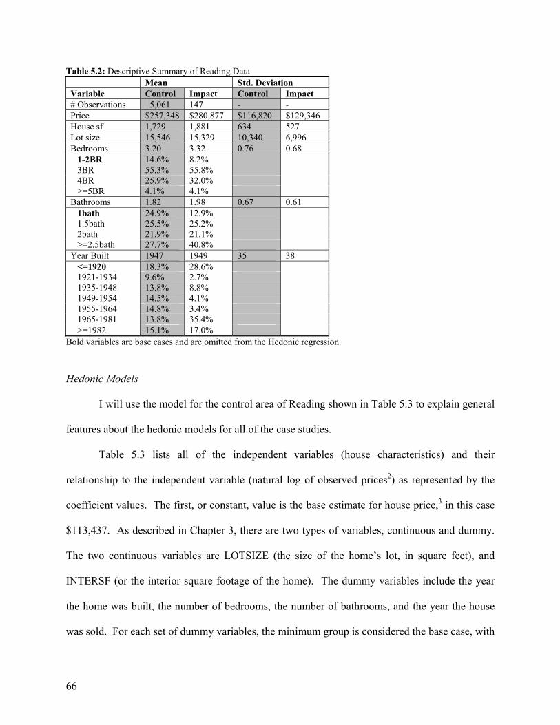
Table 5.2: Descriptive Summary of Reading Data Mean Std. Deviation Variable Control Impact Control Impact # Observations 5,061 147 - - Price $257,348 $280,877 $116,820 $129,346 House sf 1,729 1,881 634 527 Lot size 15,546 15,329 10,340 6,996 Bedrooms 3.20 3.32 0.76 0.68 1-2BR 14.6% 8.2% 3BR 55.3% 55.8% 4BR 25.9% 32.0% >=5BR 4.1% 4.1% Bathrooms 1.82 1.98 0.67 0.61 1bath 24.9% 12.9% 1.5bath 25.5% 25.2% 2bath 21.9% 21.1% >=2.5bath 27.7% 40.8% Year Built 1947 1949 35 38 <=1920 18.3% 28.6% 1921-1934 9.6% 2.7% 1935-1948 13.8% 8.8% 1949-1954 14.5% 4.1% 1955-1964 14.8% 3.4% 1965-1981 13.8% 35.4% >=1982 15.1% 17.0%
Bold variables are base cases and are omitted from the Hedonic regression.
Hedonic Models
I will use the model for the control area of Reading shown in Table 5.3 to explain general
features about the hedonic models for all of the case studies.
Table 5.3 lists all of the independent variables (house characteristics) and their
relationship to the independent variable (natural log of observed prices2) as represented by the
coefficient values. The first, or constant, value is the base estimate for house price,3 in this case
$113,437. As described in Chapter 3, there are two types of variables, continuous and dummy.
The two continuous variables are LOTSIZE (the size of the home’s lot, in square feet), and
INTERSF (or the interior square footage of the home). The dummy variables include the year
the home was built, the number of bedrooms, the number of bathrooms, and the year the house
was sold. For each set of dummy variables, the minimum group is considered the base case, with
66
a coefficient of 0, and is left out of the model. Each variable in the model has a coefficient
related to it that explains that variable’s addition (or subtraction) to the price of the home,
assuming all of the other independent variables are held constant. Because I used the natural
logarithm of the price, the unstandardized coefficient for each variable is actually describing that
variable’s contribution to the natural log of the price. In the next column, standardized
coefficient, the values are converted to a percentage format that relates to the actual sale price.
For example, in the control area of Reading, a home with one and a half baths is worth 11.9%
more than the base case house (with one bath), if all other characteristics are held constant.
Similarly, a house that sold in 1993-94 was worth 1.9% less than a house that sold in 1987-88
(the base value for year sold).
In general, the coefficients for the Reading control area make intuitive sense. Both house
and lot size are positively correlated with prices – the more is more theory of house value.
Additional bedrooms and bathrooms add value over the base case, and newer construction is
more valuable than homes built before 1921. Finally, the variable describing year sold reflects
the regional housing market over the past 18 years: decreasing home prices through the early
1990s, with a recovery in the mid- to late-90s, then rapid appreciation since 2000.
67

Table 5.3: Hedonic Model for Reading Control Area
READING CONTROL Coefficients Independent
Variables Unstandardized Standardized Standard Error t Significance
(Constant) 11.6390 - 0.0231 503.1286 0.0000 built1921-1934 0.0703 7.3% 0.0167 4.1985 0.0000 built1935-1948 0.0765 7.9% 0.0153 5.0122 0.0000 built1949-1954 0.0685 7.1% 0.0150 4.5709 0.0000 built1955-1964 0.1011 10.6% 0.0150 6.7277 0.0000 built1965-1981 0.2003 22.2% 0.0158 12.6415 0.0000 built>=1982 0.1043 11.0% 0.0165 6.3326 0.0000 sold89-90 -0.0492 -4.8% 0.0183 -2.6933 0.0071 sold91-92 -0.0917 -8.8% 0.0178 -5.1424 0.0000 sold93-94 -0.0192 -1.9% 0.0174 -1.1015 0.2707 sold95-96 0.0736 7.6% 0.0175 4.1986 0.0000 sold97-98 0.1622 17.6% 0.0176 9.2302 0.0000 sold99-00 0.3884 47.5% 0.0180 21.5984 0.0000 sold01-02 0.6585 93.2% 0.0180 36.5921 0.0000 sold03-05 0.8097 124.7% 0.0175 46.2833 0.0000 1.5bath 0.1124 11.9% 0.0124 9.0562 0.0000 2.0bath 0.0929 9.7% 0.0132 7.0142 0.0000 2.5bath 0.1862 20.5% 0.0166 11.2253 0.0000 3BR 0.0641 6.6% 0.0129 4.9672 0.0000 4BR 0.1484 16.0% 0.0163 9.0878 0.0000 >=5BR 0.1307 14.0% 0.0266 4.9143 0.0000 LOTSIZE 0.000001 N/A 0.000000 3.2951 0.0010 INTERSF 0.000126 N/A 0.000010 12.2185 0.0000 Model Summary # of Observations 5,961 Adjusted R Square 0.566 Std. Error of the Estimate 0.295519
* omitted: built<=1920, sold87-88, 1.0bath, <=2BR
Similarly, the model for the Reading impact area shows reasonable results for the
independent variables. One difference is that in this area, additional bathrooms do not seem to
add value to a house. This is not an unusual result for room number variables. The model
assumes that all other characteristics of the house, including total interior square footage, stays
the same, so the space for an additional half-bath is sacrificed from somewhere else in the base
house. The smaller size of this data set is reflected in the higher standard errors in this model,
and in general more observations lead to lower standard errors and a more dependable model.
68
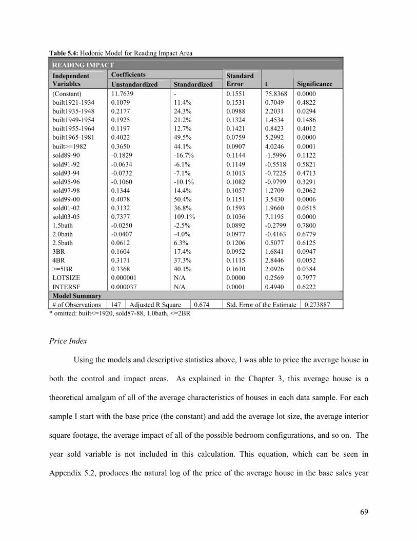
Table 5.4: Hedonic Model for Reading Impact Area
READING IMPACT Coefficients Independent
Variables Unstandardized Standardized Standard Error t Significance
(Constant) 11.7639 - 0.1551 75.8368 0.0000 built1921-1934 0.1079 11.4% 0.1531 0.7049 0.4822 built1935-1948 0.2177 24.3% 0.0988 2.2031 0.0294 built1949-1954 0.1925 21.2% 0.1324 1.4534 0.1486 built1955-1964 0.1197 12.7% 0.1421 0.8423 0.4012 built1965-1981 0.4022 49.5% 0.0759 5.2992 0.0000 built>=1982 0.3650 44.1% 0.0907 4.0246 0.0001 sold89-90 -0.1829 -16.7% 0.1144 -1.5996 0.1122 sold91-92 -0.0634 -6.1% 0.1149 -0.5518 0.5821 sold93-94 -0.0732 -7.1% 0.1013 -0.7225 0.4713 sold95-96 -0.1060 -10.1% 0.1082 -0.9799 0.3291 sold97-98 0.1344 14.4% 0.1057 1.2709 0.2062 sold99-00 0.4078 50.4% 0.1151 3.5430 0.0006 sold01-02 0.3132 36.8% 0.1593 1.9660 0.0515 sold03-05 0.7377 109.1% 0.1036 7.1195 0.0000 1.5bath -0.0250 -2.5% 0.0892 -0.2799 0.7800 2.0bath -0.0407 -4.0% 0.0977 -0.4163 0.6779 2.5bath 0.0612 6.3% 0.1206 0.5077 0.6125 3BR 0.1604 17.4% 0.0952 1.6841 0.0947 4BR 0.3171 37.3% 0.1115 2.8446 0.0052 >=5BR 0.3368 40.1% 0.1610 2.0926 0.0384 LOTSIZE 0.000001 N/A 0.0000 0.2569 0.7977 INTERSF 0.000037 N/A 0.0001 0.4940 0.6222 Model Summary # of Observations 147 Adjusted R Square 0.674 Std. Error of the Estimate 0.273887
* omitted: built<=1920, sold87-88, 1.0bath, <=2BR
Price Index
Using the models and descriptive statistics above, I was able to price the average house in
both the control and impact areas. As explained in the Chapter 3, this average house is a
theoretical amalgam of all of the average characteristics of houses in each data sample. For each
sample I start with the base price (the constant) and add the average lot size, the average interior
square footage, the average impact of all of the possible bedroom configurations, and so on. The
year sold variable is not included in this calculation. This equation, which can be seen in
Appendix 5.2, produces the natural log of the price of the average house in the base sales year
69
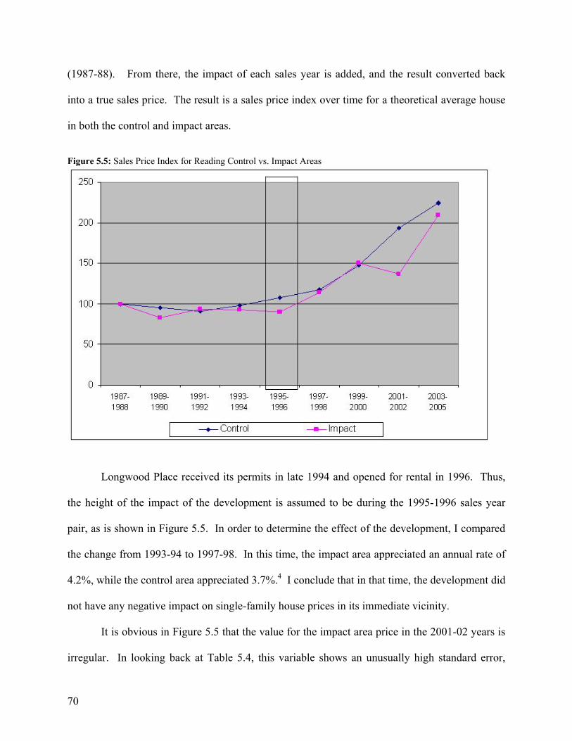
(1987-88). From there, the impact of each sales year is added, and the result converted back
into a true sales price. The result is a sales price index over time for a theoretical average house
in both the control and impact areas.
Figure 5.5: Sales Price Index for Reading Control vs. Impact Areas
Longwood Place received its permits in late 1994 and opened for rental in 1996. Thus,
the height of the impact of the development is assumed to be during the 1995-1996 sales year
pair, as is shown in Figure 5.5. In order to determine the effect of the development, I compared
the change from 1993-94 to 1997-98. In this time, the impact area appreciated an annual rate of
4.2%, while the control area appreciated 3.7%.4 I conclude that in that time, the development did
not have any negative impact on single-family house prices in its immediate vicinity.
It is obvious in Figure 5.5 that the value for the impact area price in the 2001-02 years is
irregular. In looking back at Table 5.4, this variable shows an unusually high standard error,
70
indicating that at least one data record in this group has unusual or greatly skewed properties.
Indeed, in looking back at the data, there is one transaction that has a significantly lower price
than the others, although not low enough to be removed from the sample. The impact trend
corrects in the 2003-05 sales period, when the price index returns to its previous trajectory. I
conclude that the 2001-02 blip was caused by the small data sample for that year pair and one
unusual transaction, rather than any real event in the impact zone.
Case 2: Oak Hill
Location and Impact Zone
Oak Hill is located on a mixed-use commercial strip in the town center of Ipswich.
Central Street, with a mix of residential, commercial, and small mixed-use buildings, borders the
development to the south. To the north, east, and west, the development is surrounded by single-
family homes. Oak Hill is significantly larger and denser than other uses in the areas.
Additionally, it is set up on a rise, and is quite visible from around the neighborhood.
I determined that the impact area for this case is an area of approximately 0.75 square
kilometers. The impact zone includes single-family homes as far as 600 meters or three streets
away from Oak Hill. Houses with a direct visual line to the development were included in the
impact zone, as were houses that were “trapped” by the street pattern of the neighborhood (i.e.:
have to pass the development in order to access Central Street). Additionally, houses on the
opposite side of Central Street were included in the impact zone because of the area’s
topography and the resulting visibility of the development.
71
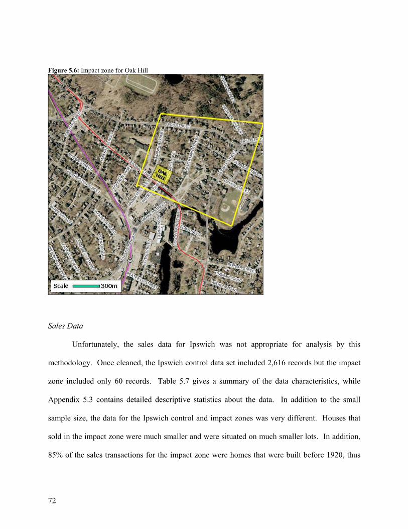
Figure 5.6: Impact zone for Oak Hill
Sales Data
Unfortunately, the sales data for Ipswich was not appropriate for analysis by this
methodology. Once cleaned, the Ipswich control data set included 2,616 records but the impact
zone included only 60 records. Table 5.7 gives a summary of the data characteristics, while
Appendix 5.3 contains detailed descriptive statistics about the data. In addition to the small
sample size, the data for the Ipswich control and impact zones was very different. Houses that
sold in the impact zone were much smaller and were situated on much smaller lots. In addition,
85% of the sales transactions for the impact zone were homes that were built before 1920, thus
72
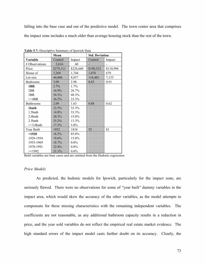
falling into the base case and out of the predictive model. The town center area that comprises
the impact zone includes a much older than average housing stock than the rest of the town.
Table 5.7: Descriptive Summary of Ipswich Data Mean Std. Deviation Variable Control Impact Control Impact # Observations 2,616 60 - - Price $279,311 $226,660 $190,532 $110,996 House sf 2,269 1,744 1,076 679 Lot size 44,606 8,037 116,481 7,135 Bedrooms 3.09 2.98 0.83 0.91 1BR 2.7% 1.7% 2BR 16.9% 26.7% 3BR 54.3% 48.3% >=4BR 26.2% 23.3% Bathrooms 2.09 1.63 0.88 0.62 1bath 22.5% 33.3% 1.5bath 14.8% 33.3% 2.0bath 20.3% 15.0% 2.5bath 25.2% 13.3% >=3.0bath 17.3% 5.0% Year Built 1952 1834 52 81 <1920 18.2% 85.0% 1920-1954 19.6% 15.0% 1955-1969 18.7% 0.0% 1970-1991 22.4% 0.0% >=1992 21.1% 0.0%
Bold variables are base cases and are omitted from the Hedonic regression.
Price Models
As predicted, the hedonic models for Ipswich, particularly for the impact zone, are
seriously flawed. There were no observations for some of “year built” dummy variables in the
impact area, which would skew the accuracy of the other variables, as the model attempts to
compensate for these missing characteristics with the remaining independent variables. The
coefficients are not reasonable, as any additional bathroom capacity results in a reduction in
price, and the year sold variables do not reflect the empirical real estate market evidence. The
high standard errors of the impact model casts further doubt on its accuracy. Clearly, the
73
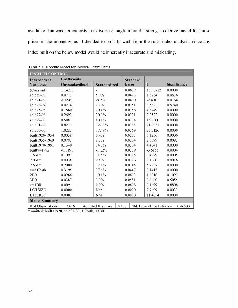
available data was not extensive or diverse enough to build a strong predictive model for house
prices in the impact zone. I decided to omit Ipswich from the sales index analysis, since any
index built on the below model would be inherently inaccurate and misleading.
Table 5.8: Hedonic Model for Ipswich Control Area
IPSWICH CONTROL Coefficients Independent
Variables Unstandardized Standardized Standard Error t Significance
(Constant) 11.4211 - 0.0689 165.8712 0.0000 sold89-90 0.0773 8.0% 0.0423 1.8284 0.0676 sold91-92 -0.0961 -9.2% 0.0400 -2.4019 0.0164 sold93-94 0.0214 2.2% 0.0381 0.5622 0.5740 sold95-96 0.1860 20.4% 0.0386 4.8249 0.0000 sold97-98 0.2692 30.9% 0.0371 7.2522 0.0000 sold99-00 0.5881 80.1% 0.0374 15.7300 0.0000 sold01-02 0.8213 127.3% 0.0385 21.3231 0.0000 sold03-05 1.0223 177.9% 0.0369 27.7126 0.0000 built1920-1954 0.0038 0.4% 0.0303 0.1256 0.9000 built1955-1969 0.0793 8.3% 0.0304 2.6079 0.0092 built1970-1991 0.1340 14.3% 0.0304 4.4041 0.0000 built>=1992 -0.1191 -11.2% 0.0339 -3.5155 0.0004 1.5bath 0.1093 11.5% 0.0315 3.4729 0.0005 2.0bath 0.0938 9.8% 0.0296 3.1660 0.0016 2.5bath 0.2000 22.1% 0.0345 5.7937 0.0000 >=3.0bath 0.3195 37.6% 0.0447 7.1415 0.0000 2BR 0.0966 10.1% 0.0603 1.6018 0.1093 3BR 0.0387 3.9% 0.0581 0.6660 0.5055 >=4BR 0.0091 0.9% 0.0608 0.1499 0.8808 LOTSIZE 0.0000 N/A 0.0000 2.9409 0.0033 INTERSF 0.0002 N/A 0.0000 11.4054 0.0000 Model Summary # of Observations 2,616 Adjusted R Square 0.478 Std. Error of the Estimate 0.46533
* omitted: built<1920, sold87-88, 1.0bath, <3BR
74
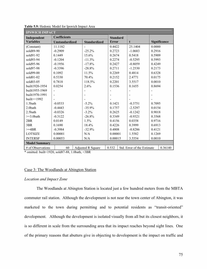
Table 5.9: Hedonic Model for Ipswich Impact Area
IPSWICH IMPACT Coefficients Independent
Variables Unstandardized Standardized Standard Error t Significance
(Constant) 11.1182 - 0.4422 25.1404 0.0000 sold89-90 -0.2909 -25.2% 0.2723 -1.0683 0.2916 sold91-92 0.1449 15.6% 0.2674 0.5418 0.5909 sold93-94 -0.1204 -11.3% 0.2274 -0.5295 0.5993 sold95-96 -0.1956 -17.8% 0.2427 -0.8059 0.4249 sold97-98 -0.3396 -28.8% 0.2711 -1.2530 0.2173 sold99-00 0.1092 11.5% 0.2269 0.4814 0.6328 sold01-02 0.5330 70.4% 0.2152 2.4771 0.0175 sold03-05 0.7818 118.5% 0.2201 3.5517 0.0010 built1920-1954 0.0254 2.6% 0.1536 0.1655 0.8694 built1955-1969 - - - - - built1970-1991 - - - - - built>=1992 - - - - - 1.5bath -0.0533 -5.2% 0.1421 -0.3751 0.7095 2.0bath -0.4443 -35.9% 0.1757 -2.5297 0.0154 2.5bath -0.0326 -3.2% 0.2625 -0.1242 0.9018 >=3.0bath -0.3122 -26.8% 0.3349 -0.9321 0.3568 2BR 0.0149 1.5% 0.4156 0.0358 0.9716 3BR 0.1690 18.4% 0.4226 0.3999 0.6913 >=4BR -0.3984 -32.9% 0.4808 -0.8286 0.4121 LOTSIZE 0.00001 N/A 0.00001 1.5582 0.1269 INTERSF 0.00053 N/A 0.00015 3.5554 0.0010 Model Summary # of Observations 60 Adjusted R Square 0.532 Std. Error of the Estimate 0.36140
* omitted: built<1920, sold87-88, 1.0bath, <3BR
Case 3: The Woodlands at Abington Station
Location and Impact Zone
The Woodlands at Abington Station is located just a few hundred meters from the MBTA
commuter rail station. Although the development is not near the town center of Abington, it was
marketed to the town during permitting and to potential residents as “transit-oriented”
development. Although the development is isolated visually from all but its closest neighbors, it
is so different in scale from the surrounding area that its impact reaches beyond sight lines. One
of the primary reasons that abutters give in objecting to development is the impact on traffic and
75
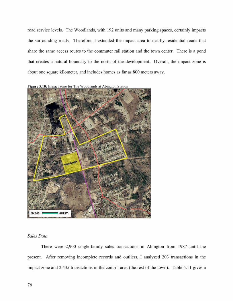
road service levels. The Woodlands, with 192 units and many parking spaces, certainly impacts
the surrounding roads. Therefore, I extended the impact area to nearby residential roads that
share the same access routes to the commuter rail station and the town center. There is a pond
that creates a natural boundary to the north of the development. Overall, the impact zone is
about one square kilometer, and includes homes as far as 800 meters away.
Figure 5.10: Impact zone for The Woodlands at Abington Station
Sales Data
There were 2,900 single-family sales transactions in Abington from 1987 until the
present. After removing incomplete records and outliers, I analyzed 203 transactions in the
impact zone and 2,435 transactions in the control area (the rest of the town). Table 5.11 gives a
76
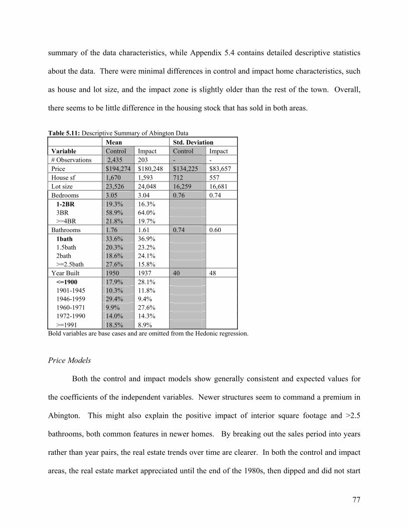
summary of the data characteristics, while Appendix 5.4 contains detailed descriptive statistics
about the data. There were minimal differences in control and impact home characteristics, such
as house and lot size, and the impact zone is slightly older than the rest of the town. Overall,
there seems to be little difference in the housing stock that has sold in both areas.
Table 5.11: Descriptive Summary of Abington Data Mean Std. Deviation Variable Control Impact Control Impact # Observations 2,435 203 - - Price $194,274 $180,248 $134,225 $83,657 House sf 1,670 1,593 712 557 Lot size 23,526 24,048 16,259 16,681 Bedrooms 3.05 3.04 0.76 0.74 1-2BR 19.3% 16.3% 3BR 58.9% 64.0% >=4BR 21.8% 19.7% Bathrooms 1.76 1.61 0.74 0.60 1bath 33.6% 36.9% 1.5bath 20.3% 23.2% 2bath 18.6% 24.1% >=2.5bath 27.6% 15.8% Year Built 1950 1937 40 48 <=1900 17.9% 28.1% 1901-1945 10.3% 11.8% 1946-1959 29.4% 9.4% 1960-1971 9.9% 27.6% 1972-1990 14.0% 14.3% >=1991 18.5% 8.9%
Bold variables are base cases and are omitted from the Hedonic regression.
Price Models
Both the control and impact models show generally consistent and expected values for
the coefficients of the independent variables. Newer structures seem to command a premium in
Abington. This might also explain the positive impact of interior square footage and >2.5
bathrooms, both common features in newer homes. By breaking out the sales period into years
rather than year pairs, the real estate trends over time are clearer. In both the control and impact
areas, the real estate market appreciated until the end of the 1980s, then dipped and did not start
77
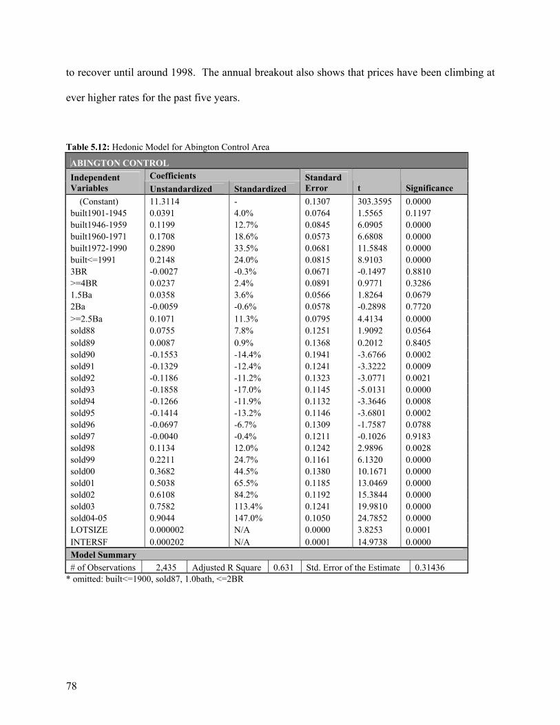
to recover until around 1998. The annual breakout also shows that prices have been climbing at
ever higher rates for the past five years.
Table 5.12: Hedonic Model for Abington Control Area
ABINGTON CONTROL Coefficients Independent
Variables Unstandardized Standardized Standard Error t Significance
(Constant) 11.3114 - 0.1307 303.3595 0.0000 built1901-1945 0.0391 4.0% 0.0764 1.5565 0.1197 built1946-1959 0.1199 12.7% 0.0845 6.0905 0.0000 built1960-1971 0.1708 18.6% 0.0573 6.6808 0.0000 built1972-1990 0.2890 33.5% 0.0681 11.5848 0.0000 built<=1991 0.2148 24.0% 0.0815 8.9103 0.0000 3BR -0.0027 -0.3% 0.0671 -0.1497 0.8810 >=4BR 0.0237 2.4% 0.0891 0.9771 0.3286 1.5Ba 0.0358 3.6% 0.0566 1.8264 0.0679 2Ba -0.0059 -0.6% 0.0578 -0.2898 0.7720 >=2.5Ba 0.1071 11.3% 0.0795 4.4134 0.0000 sold88 0.0755 7.8% 0.1251 1.9092 0.0564 sold89 0.0087 0.9% 0.1368 0.2012 0.8405 sold90 -0.1553 -14.4% 0.1941 -3.6766 0.0002 sold91 -0.1329 -12.4% 0.1241 -3.3222 0.0009 sold92 -0.1186 -11.2% 0.1323 -3.0771 0.0021 sold93 -0.1858 -17.0% 0.1145 -5.0131 0.0000 sold94 -0.1266 -11.9% 0.1132 -3.3646 0.0008 sold95 -0.1414 -13.2% 0.1146 -3.6801 0.0002 sold96 -0.0697 -6.7% 0.1309 -1.7587 0.0788 sold97 -0.0040 -0.4% 0.1211 -0.1026 0.9183 sold98 0.1134 12.0% 0.1242 2.9896 0.0028 sold99 0.2211 24.7% 0.1161 6.1320 0.0000 sold00 0.3682 44.5% 0.1380 10.1671 0.0000 sold01 0.5038 65.5% 0.1185 13.0469 0.0000 sold02 0.6108 84.2% 0.1192 15.3844 0.0000 sold03 0.7582 113.4% 0.1241 19.9810 0.0000 sold04-05 0.9044 147.0% 0.1050 24.7852 0.0000 LOTSIZE 0.000002 N/A 0.0000 3.8253 0.0001 INTERSF 0.000202 N/A 0.0001 14.9738 0.0000 Model Summary # of Observations 2,435 Adjusted R Square 0.631 Std. Error of the Estimate 0.31436
* omitted: built<=1900, sold87, 1.0bath, <=2BR
78
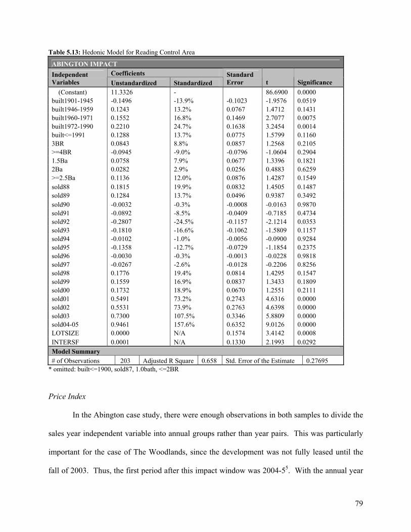
Table 5.13: Hedonic Model for Reading Control Area
ABINGTON IMPACT Coefficients Independent
Variables Unstandardized Standardized Standard Error t Significance
(Constant) 11.3326 - 86.6900 0.0000 built1901-1945 -0.1496 -13.9% -0.1023 -1.9576 0.0519 built1946-1959 0.1243 13.2% 0.0767 1.4712 0.1431 built1960-1971 0.1552 16.8% 0.1469 2.7077 0.0075 built1972-1990 0.2210 24.7% 0.1638 3.2454 0.0014 built<=1991 0.1288 13.7% 0.0775 1.5799 0.1160 3BR 0.0843 8.8% 0.0857 1.2568 0.2105 >=4BR -0.0945 -9.0% -0.0796 -1.0604 0.2904 1.5Ba 0.0758 7.9% 0.0677 1.3396 0.1821 2Ba 0.0282 2.9% 0.0256 0.4883 0.6259 >=2.5Ba 0.1136 12.0% 0.0876 1.4287 0.1549 sold88 0.1815 19.9% 0.0832 1.4505 0.1487 sold89 0.1284 13.7% 0.0496 0.9387 0.3492 sold90 -0.0032 -0.3% -0.0008 -0.0163 0.9870 sold91 -0.0892 -8.5% -0.0409 -0.7185 0.4734 sold92 -0.2807 -24.5% -0.1157 -2.1214 0.0353 sold93 -0.1810 -16.6% -0.1062 -1.5809 0.1157 sold94 -0.0102 -1.0% -0.0056 -0.0900 0.9284 sold95 -0.1358 -12.7% -0.0729 -1.1854 0.2375 sold96 -0.0030 -0.3% -0.0013 -0.0228 0.9818 sold97 -0.0267 -2.6% -0.0128 -0.2206 0.8256 sold98 0.1776 19.4% 0.0814 1.4295 0.1547 sold99 0.1559 16.9% 0.0837 1.3433 0.1809 sold00 0.1732 18.9% 0.0670 1.2551 0.2111 sold01 0.5491 73.2% 0.2743 4.6316 0.0000 sold02 0.5531 73.9% 0.2763 4.6398 0.0000 sold03 0.7300 107.5% 0.3346 5.8809 0.0000 sold04-05 0.9461 157.6% 0.6352 9.0126 0.0000 LOTSIZE 0.0000 N/A 0.1574 3.4142 0.0008 INTERSF 0.0001 N/A 0.1330 2.1993 0.0292 Model Summary # of Observations 203 Adjusted R Square 0.658 Std. Error of the Estimate 0.27695
* omitted: built<=1900, sold87, 1.0bath, <=2BR
Price Index
In the Abington case study, there were enough observations in both samples to divide the
sales year independent variable into annual groups rather than year pairs. This was particularly
important for the case of The Woodlands, since the development was not fully leased until the
fall of 2003. Thus, the first period after this impact window was 2004-55. With the annual year
79
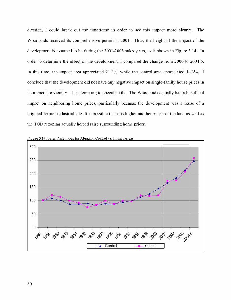
division, I could break out the timeframe in order to see this impact more clearly. The
Woodlands received its comprehensive permit in 2001. Thus, the height of the impact of the
development is assumed to be during the 2001-2003 sales years, as is shown in Figure 5.14. In
order to determine the effect of the development, I compared the change from 2000 to 2004-5.
In this time, the impact area appreciated 21.3%, while the control area appreciated 14.3%. I
conclude that the development did not have any negative impact on single-family house prices in
its immediate vicinity. It is tempting to speculate that The Woodlands actually had a beneficial
impact on neighboring home prices, particularly because the development was a reuse of a
blighted former industrial site. It is possible that this higher and better use of the land as well as
the TOD rezoning actually helped raise surrounding home prices.
Figure 5.14: Sales Price Index for Abington Control vs. Impact Areas
80
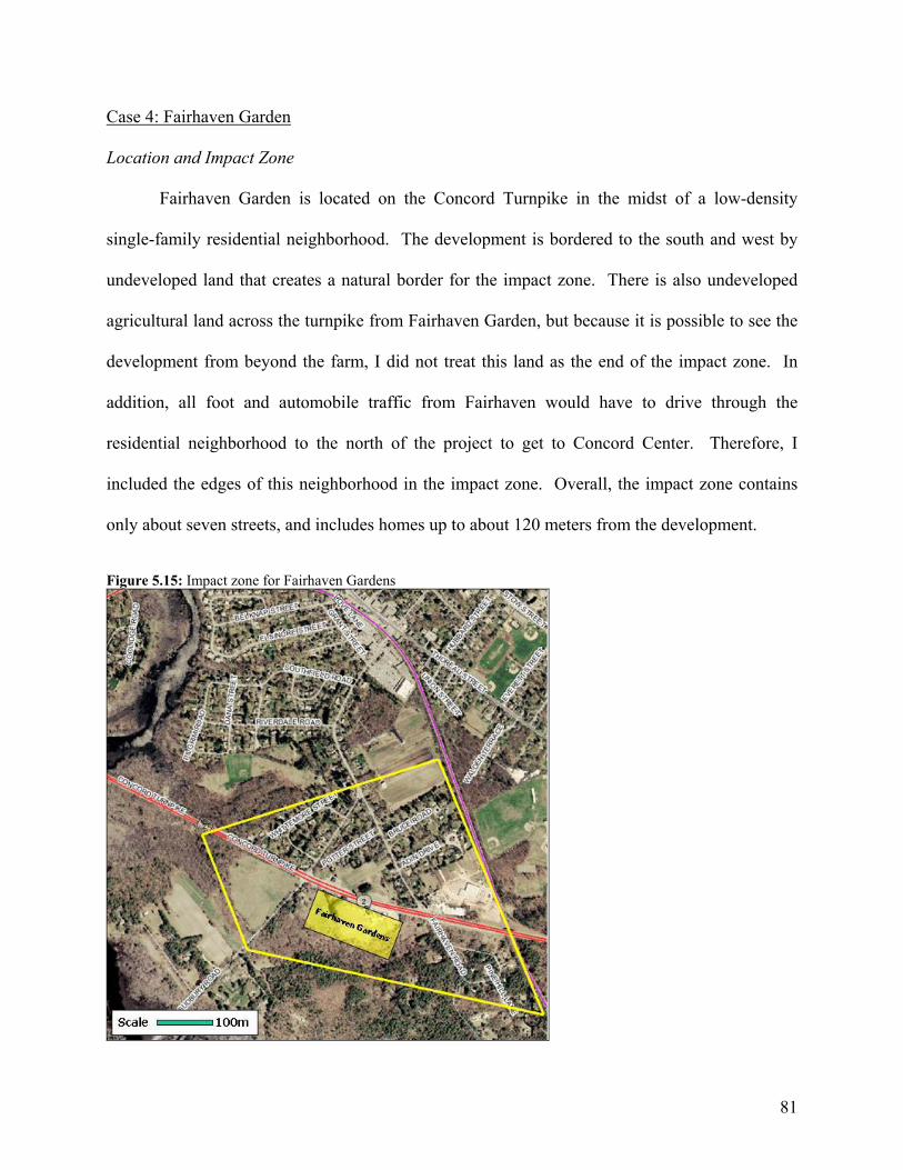
Case 4: Fairhaven Garden
Location and Impact Zone
Fairhaven Garden is located on the Concord Turnpike in the midst of a low-density
single-family residential neighborhood. The development is bordered to the south and west by
undeveloped land that creates a natural border for the impact zone. There is also undeveloped
agricultural land across the turnpike from Fairhaven Garden, but because it is possible to see the
development from beyond the farm, I did not treat this land as the end of the impact zone. In
addition, all foot and automobile traffic from Fairhaven would have to drive through the
residential neighborhood to the north of the project to get to Concord Center. Therefore, I
included the edges of this neighborhood in the impact zone. Overall, the impact zone contains
only about seven streets, and includes homes up to about 120 meters from the development.
Figure 5.15: Impact zone for Fairhaven Gardens
81
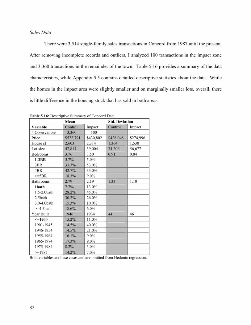
Sales Data
There were 3,514 single-family sales transactions in Concord from 1987 until the present.
After removing incomplete records and outliers, I analyzed 100 transactions in the impact zone
and 3,360 transactions in the remainder of the town. Table 5.16 provides a summary of the data
characteristics, while Appendix 5.5 contains detailed descriptive statistics about the data. While
the homes in the impact area were slightly smaller and on marginally smaller lots, overall, there
is little difference in the housing stock that has sold in both areas.
Table 5.16: Descriptive Summary of Concord Data Mean Std. Deviation Variable Control Impact Control Impact # Observations 3,360 100 - - Price $522,791 $430,802 $428,048 $274,996 House sf 2,603 2,314 1,364 1,530 Lot size 47,814 39,004 74,206 56,677 Bedrooms 3.76 3.50 0.91 0.84 1-2BR 5.7% 5.0% 3BR 33.3% 53.0% 4BR 42.7% 33.0% >=5BR 18.3% 9.0% Bathrooms 2.79 2.19 1.33 1.10 1bath 7.7% 13.0% 1.5-2.0bath 28.2% 45.0% 2.5bath 30.2% 26.0% 3.0-4.0bath 15.3% 10.0% >=4.5bath 18.6% 6.0% Year Built 1946 1934 44 46 <=1900 15.2% 11.0% 1901-1945 14.5% 40.0% 1946-1954 14.5% 21.0% 1955-1964 16.1% 9.0% 1965-1974 17.3% 9.0% 1975-1984 8.2% 3.0% >=1985 14.2% 7.0%
Bold variables are base cases and are omitted from Hedonic regression.
82
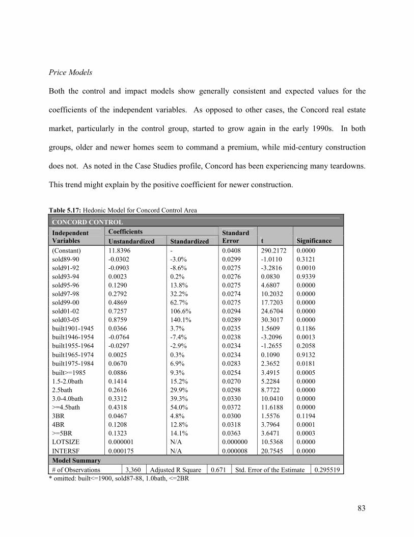
Price Models
Both the control and impact models show generally consistent and expected values for the
coefficients of the independent variables. As opposed to other cases, the Concord real estate
market, particularly in the control group, started to grow again in the early 1990s. In both
groups, older and newer homes seem to command a premium, while mid-century construction
does not. As noted in the Case Studies profile, Concord has been experiencing many teardowns.
This trend might explain by the positive coefficient for newer construction.
Table 5.17: Hedonic Model for Concord Control Area
CONCORD CONTROL Coefficients Independent
Variables Unstandardized Standardized Standard Error t Significance
(Constant) 11.8396 - 0.0408 290.2172 0.0000 sold89-90 -0.0302 -3.0% 0.0299 -1.0110 0.3121 sold91-92 -0.0903 -8.6% 0.0275 -3.2816 0.0010 sold93-94 0.0023 0.2% 0.0276 0.0830 0.9339 sold95-96 0.1290 13.8% 0.0275 4.6807 0.0000 sold97-98 0.2792 32.2% 0.0274 10.2032 0.0000 sold99-00 0.4869 62.7% 0.0275 17.7203 0.0000 sold01-02 0.7257 106.6% 0.0294 24.6704 0.0000 sold03-05 0.8759 140.1% 0.0289 30.3017 0.0000 built1901-1945 0.0366 3.7% 0.0235 1.5609 0.1186 built1946-1954 -0.0764 -7.4% 0.0238 -3.2096 0.0013 built1955-1964 -0.0297 -2.9% 0.0234 -1.2655 0.2058 built1965-1974 0.0025 0.3% 0.0234 0.1090 0.9132 built1975-1984 0.0670 6.9% 0.0283 2.3652 0.0181 built>=1985 0.0886 9.3% 0.0254 3.4915 0.0005 1.5-2.0bath 0.1414 15.2% 0.0270 5.2284 0.0000 2.5bath 0.2616 29.9% 0.0298 8.7722 0.0000 3.0-4.0bath 0.3312 39.3% 0.0330 10.0410 0.0000 >=4.5bath 0.4318 54.0% 0.0372 11.6188 0.0000 3BR 0.0467 4.8% 0.0300 1.5576 0.1194 4BR 0.1208 12.8% 0.0318 3.7964 0.0001 >=5BR 0.1323 14.1% 0.0363 3.6471 0.0003 LOTSIZE 0.000001 N/A 0.000000 10.5368 0.0000 INTERSF 0.000175 N/A 0.000008 20.7545 0.0000 Model Summary # of Observations 3,360 Adjusted R Square 0.671 Std. Error of the Estimate 0.295519
* omitted: built<=1900, sold87-88, 1.0bath, <=2BR
83
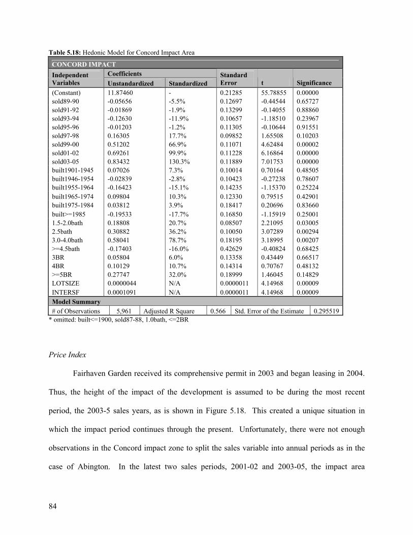
Table 5.18: Hedonic Model for Concord Impact Area
CONCORD IMPACT Coefficients Independent
Variables Unstandardized Standardized Standard Error t Significance
(Constant) 11.87460 - 0.21285 55.78855 0.00000 sold89-90 -0.05656 -5.5% 0.12697 -0.44544 0.65727 sold91-92 -0.01869 -1.9% 0.13299 -0.14055 0.88860 sold93-94 -0.12630 -11.9% 0.10657 -1.18510 0.23967 sold95-96 -0.01203 -1.2% 0.11305 -0.10644 0.91551 sold97-98 0.16305 17.7% 0.09852 1.65508 0.10203 sold99-00 0.51202 66.9% 0.11071 4.62484 0.00002 sold01-02 0.69261 99.9% 0.11228 6.16864 0.00000 sold03-05 0.83432 130.3% 0.11889 7.01753 0.00000 built1901-1945 0.07026 7.3% 0.10014 0.70164 0.48505 built1946-1954 -0.02839 -2.8% 0.10423 -0.27238 0.78607 built1955-1964 -0.16423 -15.1% 0.14235 -1.15370 0.25224 built1965-1974 0.09804 10.3% 0.12330 0.79515 0.42901 built1975-1984 0.03812 3.9% 0.18417 0.20696 0.83660 built>=1985 -0.19533 -17.7% 0.16850 -1.15919 0.25001 1.5-2.0bath 0.18808 20.7% 0.08507 2.21095 0.03005 2.5bath 0.30882 36.2% 0.10050 3.07289 0.00294 3.0-4.0bath 0.58041 78.7% 0.18195 3.18995 0.00207 >=4.5bath -0.17403 -16.0% 0.42629 -0.40824 0.68425 3BR 0.05804 6.0% 0.13358 0.43449 0.66517 4BR 0.10129 10.7% 0.14314 0.70767 0.48132 >=5BR 0.27747 32.0% 0.18999 1.46045 0.14829 LOTSIZE 0.0000044 N/A 0.0000011 4.14968 0.00009 INTERSF 0.0001091 N/A 0.0000011 4.14968 0.00009 Model Summary # of Observations 5,961 Adjusted R Square 0.566 Std. Error of the Estimate 0.295519
* omitted: built<=1900, sold87-88, 1.0bath, <=2BR
Price Index
Fairhaven Garden received its comprehensive permit in 2003 and began leasing in 2004.
Thus, the height of the impact of the development is assumed to be during the most recent
period, the 2003-5 sales years, as is shown in Figure 5.18. This created a unique situation in
which the impact period continues through the present. Unfortunately, there were not enough
observations in the Concord impact zone to split the sales variable into annual periods as in the
case of Abington. In the latest two sales periods, 2001-02 and 2003-05, the impact area
84
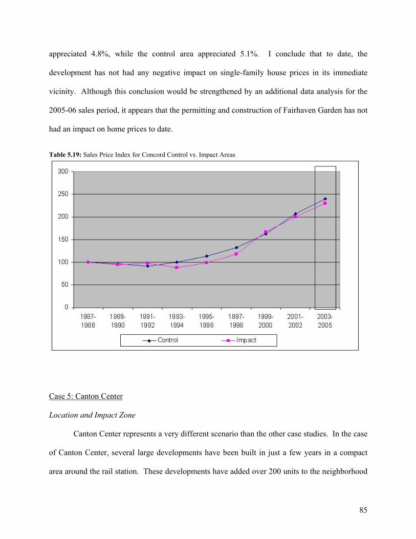
appreciated 4.8%, while the control area appreciated 5.1%. I conclude that to date, the
development has not had any negative impact on single-family house prices in its immediate
vicinity. Although this conclusion would be strengthened by an additional data analysis for the
2005-06 sales period, it appears that the permitting and construction of Fairhaven Garden has not
had an impact on home prices to date.
Table 5.19: Sales Price Index for Concord Control vs. Impact Areas
Case 5: Canton Center
Location and Impact Zone
Canton Center represents a very different scenario than the other case studies. In the case
of Canton Center, several large developments have been built in just a few years in a compact
area around the rail station. These developments have added over 200 units to the neighborhood
85

and from all accounts, completely changed the nature of Canton Center. Therefore, I argue that
the impact zone comprises the majority of the single-family homes within the overlay district.
This is an oddly-shaped area bordered on the east by Forge Pond and the west and south by
commercial/industrial land. Overall, the impact zone is about 800 by 800 meters, and includes
homes as far as 300 meters away from one of the developments.
Figure 5.20: Impact zone for Canton Center Economic Development Overlay District
Sales Data
There were 3,754 single-family sales transactions in Canton from 1987 until the present.
After removing incomplete records and outliers, I analyzed 96 transactions in the impact zone
and 3,102 transactions in the rest of the town. Table 5.21 provides a summary of the data
86
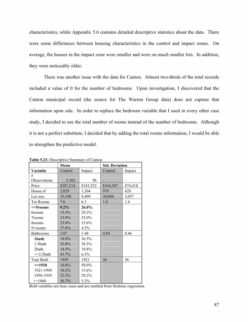
characteristics, while Appendix 5.6 contains detailed descriptive statistics about the data. There
were some differences between housing characteristics in the control and impact zones. On
average, the houses in the impact zone were smaller and were on much smaller lots. In addition,
they were noticeably older.
There was another issue with the data for Canton. Almost two-thirds of the total records
included a value of 0 for the number of bedrooms. Upon investigation, I discovered that the
Canton municipal record (the source for The Warren Group data) does not capture that
information upon sale. In order to replace the bedroom variable that I used in every other case
study, I decided to use the total number of rooms instead of the number of bedrooms. Although
it is not a perfect substitute, I decided that by adding the total rooms information, I would be able
to strengthen the predictive model.
Table 5.21: Descriptive Summary of Canton Mean Std. Deviation Variable Control Impact Control Impact # Observations 3,102 96 - - Price $287,214 $183,522 $164,307 $74,418 House sf 2,029 1,504 979 429 Lot size 25,198 8,490 20,094 3,057 Tot Rooms 7.6 6.3 1.8 1.4 <=5rooms 9.2% 26.0% 6rooms 15.3% 29.2% 7rooms 23.9% 25.0% 8rooms 23.8% 15.6% 9+rooms 27.8% 4.2% Bathrooms 2.07 1.48 0.84 0.46 1bath 18.0% 36.5% 1.5bath 23.8% 38.5% 2bath 14.5% 18.8% >=2.5bath 43.7% 6.3% Year Built 1959 1921 36 36 <=1920 10.8% 50.0% 1921-1949 10.2% 15.6% 1950-1959 22.3% 29.2% >=1960 56.7% 5.2%
Bold variables are base cases and are omitted from Hedonic regression.
87
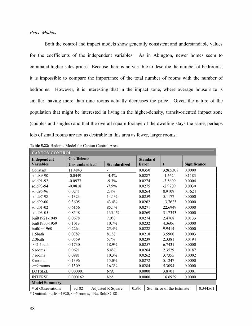
Price Models
Both the control and impact models show generally consistent and understandable values
for the coefficients of the independent variables. As in Abington, newer homes seem to
command higher sales prices. Because there is no variable to describe the number of bedrooms,
it is impossible to compare the importance of the total number of rooms with the number of
bedrooms. However, it is interesting that in the impact zone, where average house size is
smaller, having more than nine rooms actually decreases the price. Given the nature of the
population that might be interested in living in the higher-density, transit-oriented impact zone
(couples and singles) and that the overall square footage of the dwelling stays the same, perhaps
lots of small rooms are not as desirable in this area as fewer, larger rooms.
Table 5.22: Hedonic Model for Canton Control Area
CANTON CONTROL Coefficients Independent
Variables Unstandardized Standardized Standard Error t Significance
Constant 11.4843 - 0.0350 328.5308 0.0000 sold89-90 -0.0449 -4.4% 0.0287 -1.5624 0.1183 sold91-92 -0.0977 -9.3% 0.0274 -3.5609 0.0004 sold93-94 -0.0818 -7.9% 0.0275 -2.9709 0.0030 sold95-96 0.0241 2.4% 0.0264 0.9109 0.3624 sold97-98 0.1323 14.1% 0.0259 5.1177 0.0000 sold99-00 0.3605 43.4% 0.0262 13.7623 0.0000 sold01-02 0.6156 85.1% 0.0271 22.6949 0.0000 sold03-05 0.8548 135.1% 0.0269 31.7343 0.0000 built1921-1949 0.0678 7.0% 0.0274 2.4768 0.0133 built1950-1959 0.1013 10.7% 0.0232 4.3606 0.0000 built>=1960 0.2264 25.4% 0.0228 9.9414 0.0000 1.5bath 0.0782 8.1% 0.0218 3.5900 0.0003 2.0bath 0.0559 5.7% 0.0239 2.3381 0.0194 >=2.5bath 0.1730 18.9% 0.0257 6.7431 0.0000 6 rooms 0.0621 6.4% 0.0264 2.3529 0.0187 7 rooms 0.0981 10.3% 0.0262 3.7355 0.0002 8 rooms 0.1396 15.0% 0.0272 5.1247 0.0000 >=9 rooms 0.1509 16.3% 0.0284 5.3094 0.0000 LOTSIZE 0.000001 N/A 0.0000 3.8701 0.0001 INTERSF 0.000162 N/A 0.0000 16.6929 0.0000 Model Summary # of Observations 3,102 Adjusted R Square 0.596 Std. Error of the Estimate 0.344561
* Omitted: built<=1920, <=5 rooms, 1Ba, Sold87-88
88
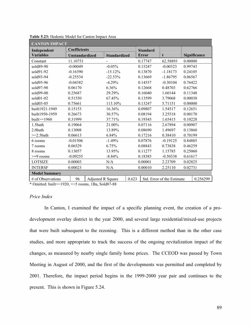
Table 5.23: Hedonic Model for Canton Impact Area
CANTON IMPACT Coefficients Independent
Variables Unstandardized Standardized Standard Error t Significance
Constant 11.10751 - 0.17747 62.58893 0.00000 sold89-90 -0.00049 -0.05% 0.15247 -0.00323 0.99743 sold91-92 -0.16390 -15.12% 0.13870 -1.18173 0.24105 sold93-94 -0.25534 -22.53% 0.13669 -1.86795 0.06567 sold95-96 -0.04382 -4.29% 0.14557 -0.30104 0.76422 sold97-98 0.06170 6.36% 0.12668 0.48703 0.62766 sold99-00 0.25687 29.29% 0.16040 1.60144 0.11348 sold01-02 0.51550 67.45% 0.13599 3.79068 0.00030 sold03-05 0.75661 113.10% 0.13247 5.71151 0.00000 built1921-1949 0.15153 16.36% 0.09807 1.54517 0.12651 built1950-1959 0.26673 30.57% 0.08194 3.25518 0.00170 built>=1960 0.31999 37.71% 0.19345 1.65415 0.10228 1.5bath 0.19064 21.00% 0.07116 2.67894 0.00907 2.0bath 0.13008 13.89% 0.08690 1.49697 0.13860 >=2.5bath 0.06613 6.84% 0.17216 0.38410 0.70199 6 rooms -0.01506 -1.49% 0.07876 -0.19125 0.84885 7 rooms 0.06529 6.75% 0.08843 0.73838 0.46259 8 rooms 0.13057 13.95% 0.11277 1.15785 0.25060 >=9 rooms -0.09255 -8.84% 0.18385 -0.50338 0.61617 LOTSIZE 0.00003 N/A 0.00001 2.23709 0.02825 INTERSF 0.00023 N/A 0.00010 2.25110 0.02731 Model Summary # of Observations 96 Adjusted R Square 0.623 Std. Error of the Estimate 0.256299
* Omitted: built<=1920, <=5 rooms, 1Ba, Sold87-88
Price Index
In Canton, I examined the impact of a specific planning event, the creation of a pro-
development overlay district in the year 2000, and several large residential/mixed-use projects
that were built subsequent to the rezoning. This is a different method than in the other case
studies, and more appropriate to track the success of the ongoing revitalization impact of the
changes, as measured by nearby single family home prices. The CCEOD was passed by Town
Meeting in August of 2000, and the first of the developments was permitted and completed by
2001. Therefore, the impact period begins in the 1999-2000 year pair and continues to the
present. This is shown in Figure 5.24.
89
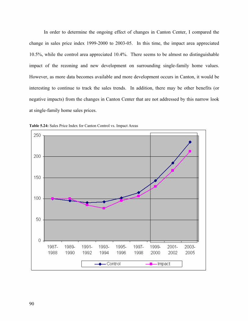
In order to determine the ongoing effect of changes in Canton Center, I compared the
change in sales price index 1999-2000 to 2003-05. In this time, the impact area appreciated
10.5%, while the control area appreciated 10.4%. There seems to be almost no distinguishable
impact of the rezoning and new development on surrounding single-family home values.
However, as more data becomes available and more development occurs in Canton, it would be
interesting to continue to track the sales trends. In addition, there may be other benefits (or
negative impacts) from the changes in Canton Center that are not addressed by this narrow look
at single-family home sales prices.
Table 5.24: Sales Price Index for Canton Control vs. Impact Areas
90
1 Appendix 5.1 contains a full list of independent variables that were used. 2 The natural logarithm of the sales price is defined as en = x, where e = 2.71828… and x = the numeric sales price. For example, the natural logarithm of $100,000 is 11.513 (100,000 = 2.7182811.513). The natural logarithm of the sales price is used as the dependent variable in all of the models in this study because these values reduce the difference between values and thus the weight of any wildly different sales prices. For example, for sales prices of $100,000 and $2,100,000, the natural logarithms are 11.513 and 14.557 respectively. 3 Because the output of the models refers to the natural logarithm of price, we must take the antilog of these numbers to interpret the result as a price. For example, the antilog of the Reading control constant, 11.639, is e11.639 = price = $113,437. 4 Appreciation is expressed as the Compound Annual Growth Rate, which is calculated as
CAGR = (end value)/(beginning value)(1/# years)-1)
5 I kept 2004 and 2005 transactions together because the transaction records only included sales in the first few months of 2005. A 2005 only sample would have been too small and irregular for this study.
91

92
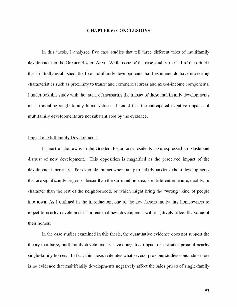
CHAPTER 6: CONCLUSIONS
In this thesis, I analyzed five case studies that tell three different tales of multifamily
development in the Greater Boston Area. While none of the case studies met all of the criteria
that I initially established, the five multifamily developments that I examined do have interesting
characteristics such as proximity to transit and commercial areas and mixed-income components.
I undertook this study with the intent of measuring the impact of these multifamily developments
on surrounding single-family home values. I found that the anticipated negative impacts of
multifamily developments are not substantiated by the evidence.
Impact of Multifamily Developments
In most of the towns in the Greater Boston area residents have expressed a distaste and
distrust of new development. This opposition is magnified as the perceived impact of the
development increases. For example, homeowners are particularly anxious about developments
that are significantly larger or denser than the surrounding area, are different in tenure, quality, or
character than the rest of the neighborhood, or which might bring the “wrong” kind of people
into town. As I outlined in the introduction, one of the key factors motivating homeowners to
object to nearby development is a fear that new development will negatively affect the value of
their homes.
In the case studies examined in this thesis, the quantitative evidence does not support the
theory that large, multifamily developments have a negative impact on the sales price of nearby
single-family homes. In fact, this thesis reiterates what several previous studies conclude - there
is no evidence that multifamily developments negatively affect the sales prices of single-family
93
homes within the impact area. In each of the four case studies that had solid quantitative results,
the only sizable difference between the annual growth in the sales price of the average home in
the impact zone and the average home in the rest of the town during and after the permitting and
construction of the case development was in Abington, and it was positive in favor of the impact
zone.1
Figure 6.1: Compound Annual Growth Rate – Impact vs. Control areas of the five case study towns
4.64%
14.34
%
7.80%
13.15
%
5.33%
7.34%
13.31
%
21.31
%
0%
5%
10%
15%
20%
25%
Reading Abington Concord Canton
Compound Annual Growth Rate
ControlImpact
Community Response and Growth Planning
Despite these conclusions, my interviews indicate that this kind of evidence is but a
starting point for a larger process of discourse and education. In discussions with planners, town
officials and developers, the overwhelming tale of each development was one of cooperation and
94
collaboration, negotiation and compromise, with the end result a development that turned out to
be much better than everyone expected. In both Concord and Abington, town officials claimed
that the ease of the comprehensive permit process and the success of the development would
make them more likely to proactively seek out similar developments, and in all cases, municipal
officials agreed that a successful example development was an extremely effective way to refute
NIMBY attitudes.
However, responses from the public were less unequivocal. From discussions with
neighbors, it seems that residents see no irony in embracing a completed development at the
same time that they condemn the next one. All of the residents surveyed in Canton, were
enthusiastic about the changes in Canton Center. One longtime resident said that the
proliferation of new businesses “brought her downtown again.” Another new Canton resident
confirmed that it was her home’s proximity to transit that attracted her to Canton Center. In both
Ipswich and Reading, the projects were a source of pride for residents. A woman in Reading
told me that Longwood Place is a “great resource for the community, and a terrific neighbor.”
Her only complaint was that her houseguests weren’t allowed to park in the Longwood parking
lot. One resident of Concord who lives across the road from the Fairhaven Garden project
expressed his surprise and pleasure at the development. He stated that, “…once construction was
done, I didn’t even notice those apartments. Those buildings don’t bother me, and I don’t notice
any additional traffic or problems from the people who live there.”
However, he continued that one apartment development is enough and because Concord
is “almost developed to capacity,” he would have a hard time supporting additional
developments like Fairhaven Gardens. In a town that has many acres of undeveloped land, a
minimum lot size of two acres and an average density of 0.39 units per acre, his perception of
95

maximum build out is surprising and, I would argue, inaccurate. It seems that despite the
presence of successful multifamily developments in town, and despite acknowledgement of these
existing successes, public dislike of development continues. One Beacon Residential Properties
employee who worked on The Woodlands at Abington Station says it best: “People would rather
have woods than any kind of development.”
Suggestions for Future Research
It is tempting to conclude that with this addition to previous studies (Ritchay and
Weinrobe, 2004 and Weinstein, 2002), the evidence is overwhelming that there is no negative
impact of multifamily and mixed-income housing on surrounding home prices. However, I
believe that there are limitations to this body of research that invite further investigation and
suggest ideas for additional research.
First of all, both this and Ritchay and Weinrobe’s 2004 thesis focus on the Eastern
Massachusetts residential real estate market in a time of remarkable growth, while Weinstein’s
(2002) study looks at the San Francisco Bay area in a similarly appreciating market. The
residential market has been increasing astronomically in the Greater Boston Area, particularly in
the past five years, and I would argue that economic nuances might be revealed in an equilibrium
market that are masked in the current market. For example, in a more tepid real estate market,
proximity to a negative land use might affect house price more than in a market where
everything sells for top dollar, regardless of its location. Conducting this type of study with
similar methodology in a slower residential market would be an interesting juxtaposition to this
group of studies.
96
Secondly, in this research, I found it difficult to be confident that I was identifying all of
the critical information about a specific case study. Even though I spoke to myriad constituents
about some very controversial topics, the fog of memory seems to have blunted their accounts of
the history of the permitting process and public reaction. In some cases, the public record cast
suspicion on these rosy accounts, but in far more cases, the public record was incomplete or
nonexistent. Additionally, in a study that uses interviews and the written record to paint the story
of a development, some factors will always be left out. I think that a valuable long-term study
would follow one development from cradle to grave, combining a qualitative record of the
process and the evolution of public opinion with a quantitative follow-up study of the impacts.
Third, I would suggest that the price trends analyzed in this and Ritchay and Weinrobe’s
thesis continue to be monitored. There are claims that multifamily developments, particularly
those with a mixed-income population are constructed poorly, are not maintained well, and
develop into eyesores, becoming a growing negative impact on the neighborhood. To explore
this, the price index of the impact and control zones could be tracked on an ongoing basis, with
notation of renovations to the development or other major events.
Finally, I think that a more expansive analysis of the changes that have happened in areas
like Canton Center is merited. Canton is the only one of my case studies where an intentional
zoning change was implemented to create a growth district. I think that a study quantifying the
impacts of the CCEDO district in Canton Center could serve as a powerful testimony to this type
of growth. I found that it was the most interesting and vibrant of the case studies to visit. An
analysis of not only the economic impacts on surrounding property, but also a benefit/cost
analysis of the zoning change to the town and a qualitative analysis of perceptions about the area
would be interesting.
97
A well-designed housing price study is complex and time consuming. Freeman and
Botein2 note, “As with most nonexperimental social science research, the most vexing problem is
designing methods that can satisfactorily answer the question at hand.”1 Case studies must be
chosen carefully and impact areas determined by extensive investigation of actual neighborhood
boundaries rather than by mere linear distance or the convenience of census or other divisions.
All future research must avoid the methodological pitfalls that plagued earlier studies and they
must explicitly deal with the unique design of case study developments and peculiarities of the
towns in question.
In a way, conducting studies with the intent of allaying fears about development is a
thankless Sisyphean task. To paraphrase one member of the housing community, each time you
chip away at one misconception about development, people will find another one to introduce. If
and when we ever succeed in “proving” that multifamily developments cause no negative
impacts on surrounding single-family home values, another fear will take its place. However,
only by adding to the body of evidence well-designed studies with clear conclusions can we
begin to refute the fear of negative impacts of development. While this evidence may not
completely take away the risk adverse mindset of the NIMBYist, it may begin to persuade
homevoters to take a chance on well-designed, well-planned developments.
1 In Abington, The Woodlands development is a reuse of a previously industrial site and thus might represent a positive improvement to the neighbors. 2 Lance Freeman and Hilary Botein (2002), Subsidized Housing and Neighborhood Impacts: A Theoretical Discussion and Review of the Evidence, Journal of Planning Literature, 16(3), p.366.
98
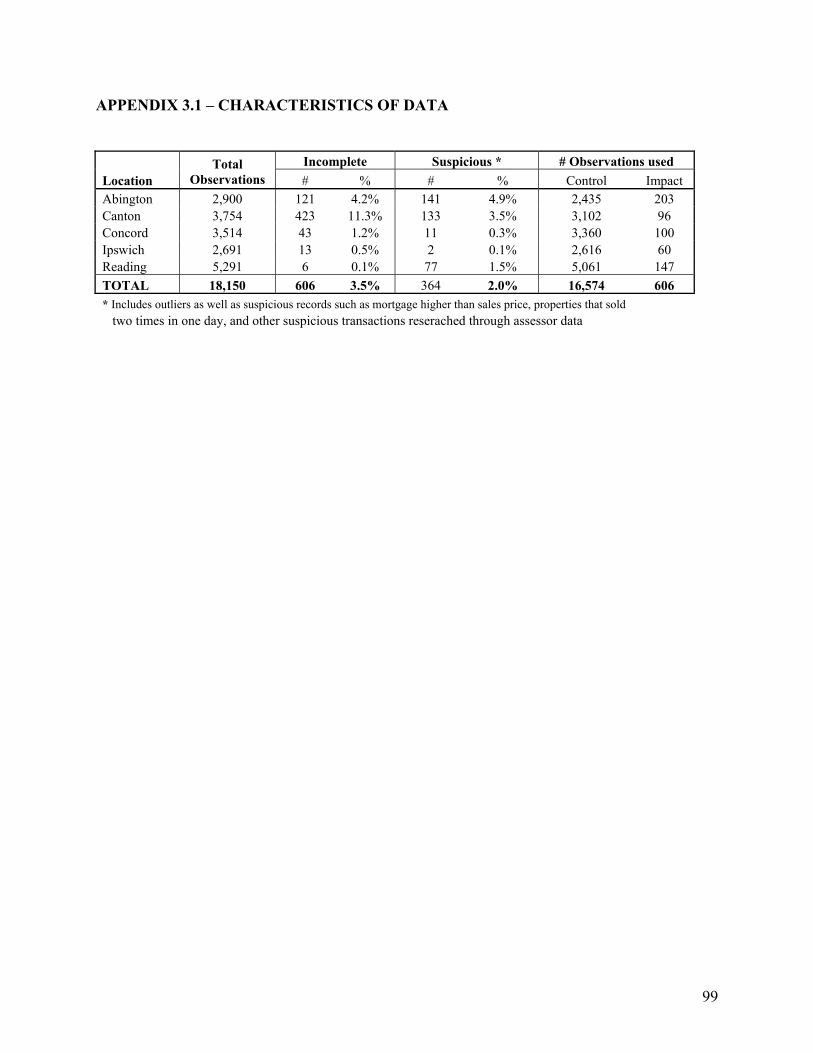
APPENDIX 3.1 – CHARACTERISTICS OF DATA Incomplete Suspicious * # Observations used Location
Total Observations # % # % Control Impact
Abington 2,900 121 4.2% 141 4.9% 2,435 203 Canton 3,754 423 11.3% 133 3.5% 3,102 96 Concord 3,514 43 1.2% 11 0.3% 3,360 100 Ipswich 2,691 13 0.5% 2 0.1% 2,616 60 Reading 5,291 6 0.1% 77 1.5% 5,061 147 TOTAL 18,150 606 3.5% 364 2.0% 16,574 606 * Includes outliers as well as suspicious records such as mortgage higher than sales price, properties that sold two times in one day, and other suspicious transactions reserached through assessor data
99
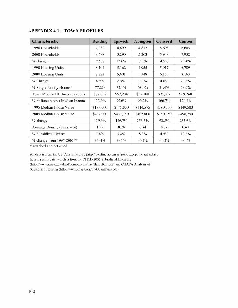
APPENDIX 4.1 – TOWN PROFILES
Characteristic Reading Ipswich Abington Concord Canton 1990 Households 7,932 4,699 4,817 5,693 6,605
2000 Households 8,688 5,290 5,263 5,948 7,952
% change 9.5% 12.6% 7.9% 4.5% 20.4%
1990 Housing Units 8,104 5,162 4,955 5,917 6,789
2000 Housing Units 8,823 5,601 5,348 6,153 8,163
% Change 8.9% 8.5% 7.9% 4.0% 20.2%
% Single Family Homes* 77.2% 72.1% 69.0% 81.4% 68.0%
Town Median HH Income (2000) $77,059 $57,284 $57,100 $95,897 $69,260
% of Boston Area Median Income 133.9% 99.6% 99.2% 166.7% 120.4%
1995 Median House Value $178,000 $175,000 $114,575 $390,000 $149,500
2005 Median House Value $427,000 $431,750 $405,000 $750,750 $498,750
% change 139.9% 146.7% 253.5% 92.5% 233.6%
Average Density (units/acre) 1.39 0.26 0.84 0.39 0.67
% Subsidized Units* 7.8% 7.8% 8.3% 4.5% 10.2%
% change from 1997-2005** +3-4% +<1% +>5% +1-2% +<1% * attached and detached All data is from the US Census website (http://factfinder.census.gov), except the subsidized housing units data, which is from the DHCD 2005 Subsidized Inventory (http://www.mass.gov/dhcd/components/hac/HsInvRev.pdf) and CHAPA Analysis of Subsidized Housing (http://www.chapa.org/0540banalysis.pdf).
100
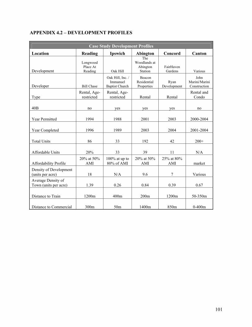
APPENDIX 4.2 – DEVELOPMENT PROFILES
Case Study Development Profiles Location Reading Ipswich Abington Concord Canton
Development
Longwood Place At Reading Oak Hill
The Woodlands at
Abington Station
FairHaven Gardens Various
Developer Bill Chase
Oak Hill, Inc. / Immanuel
Baptist Church
Beacon Residential Properties
Ryan Development
John Marini/Marini Construction
Type Rental, Age-
restricted Rental, Age-
restricted Rental Rental Rental and
Condo
40B no yes yes yes no
Year Permitted 1994 1988 2001 2003 2000-2004
Year Completed 1996 1989 2003 2004 2001-2004
Total Units 86 33 192 42 200+
Affordable Units 20% 33 39 11 N/A
Affordability Profile 20% at 50%
AMI 100% at up to 80% of AMI
20% at 50% AMI
25% at 80% AMI market
Density of Development (units per acre) 18 N/A 9.6 7 Various Average Density of Town (units per acre) 1.39 0.26 0.84 0.39 0.67
Distance to Train 1200m 400m 200m 1200m 50-350m
Distance to Commercial 300m 50m 1400m 850m 0-400m
101
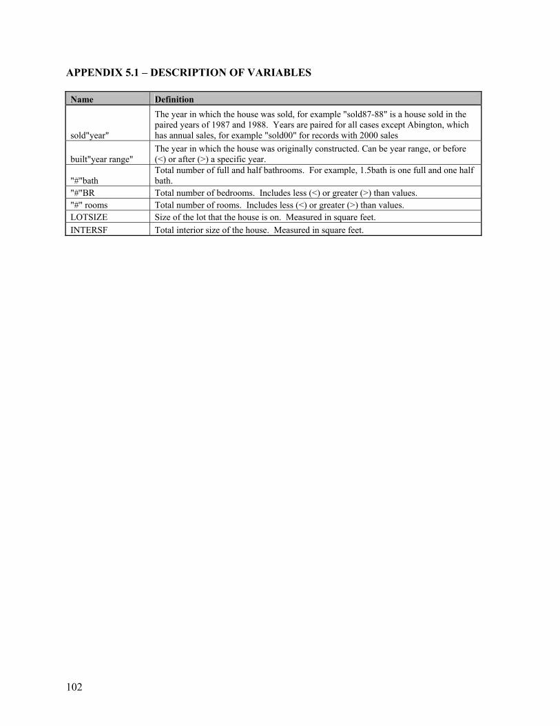
APPENDIX 5.1 – DESCRIPTION OF VARIABLES Name Definition
sold"year"
The year in which the house was sold, for example "sold87-88" is a house sold in the paired years of 1987 and 1988. Years are paired for all cases except Abington, which has annual sales, for example "sold00" for records with 2000 sales
built"year range" The year in which the house was originally constructed. Can be year range, or before (<) or after (>) a specific year.
"#"bath Total number of full and half bathrooms. For example, 1.5bath is one full and one half bath.
"#"BR Total number of bedrooms. Includes less (<) or greater (>) than values. "#" rooms Total number of rooms. Includes less (<) or greater (>) than values. LOTSIZE Size of the lot that the house is on. Measured in square feet. INTERSF Total interior size of the house. Measured in square feet.
102
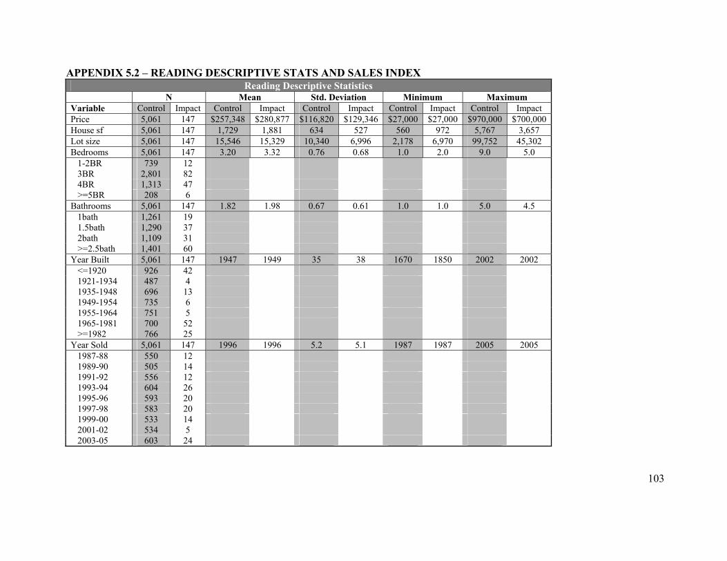
APPENDIX 5.2 – READING DESCRIPTIVE STATS AND SALES INDEX Reading Descriptive Statistics
N Mean Std. Deviation Minimum MaximumVariable Control Impact Control Impact Control Impact Control Impact Control Impact Price 5,061 147 $257,348 $280,877 $116,820 $129,346 $27,000 $27,000 $970,000 $700,000House sf 5,061 147 1,729 1,881 634 527 560 972 5,767 3,657 Lot size 5,061 147 15,546 15,329 10,340 6,996 2,178 6,970 99,752 45,302 Bedrooms 5,061 147 3.20 3.32 0.76 0.68 1.0 2.0 9.0 5.0 1-2BR 739 12 3BR 2,801 82 4BR 1,313 47 >=5BR 208 6 Bathrooms 5,061 147 1.82 1.98 0.67 0.61 1.0 1.0 5.0 4.5 1bath 1,261 19 1.5bath 1,290 37 2bath 1,109 31 >=2.5bath 1,401 60 Year Built 5,061 147 1947 1949 35 38 1670 1850 2002 2002 <=1920 926 42 1921-1934 487 4 1935-1948 696 13 1949-1954 735 6 1955-1964 751 5 1965-1981 700 52 >=1982 766 25 Year Sold 5,061 147 1996 1996 5.2 5.1 1987 1987 2005 2005 1987-88 550 12 1989-90 505 14 1991-92 556 12 1993-94 604 26 1995-96 593 20 1997-98 583 20 1999-00 533 14 2001-02 534 5 2003-05 603 24
103
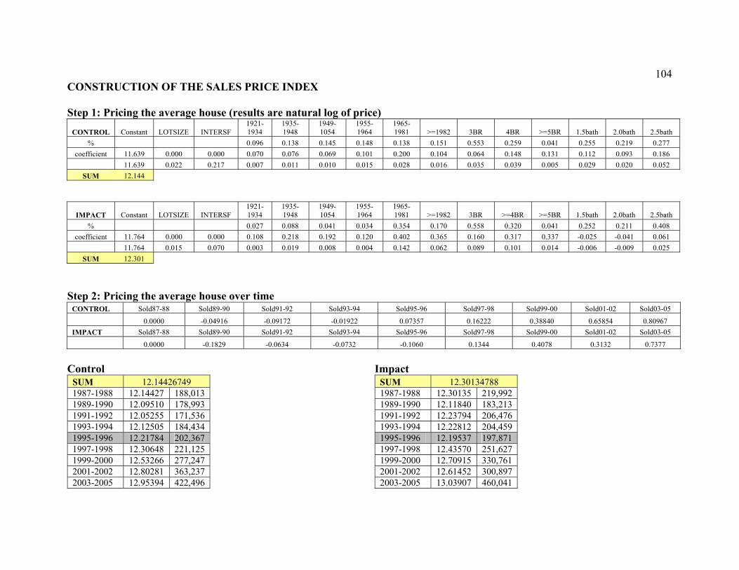
104 CONSTRUCTION OF THE SALES PRICE INDEX Step 1: Pricing the average house (results are natural log of price)
CONTROL Constant LOTSIZE INTERSF1921-1934
1935-1948
1949-1054
1955-1964
1965-1981 >=1982 3BR 4BR >=5BR 1.5bath 2.0bath 2.5bath
% 0.096 0.138 0.145 0.148 0.138 0.151 0.553 0.259 0.041 0.255 0.219 0.277coefficient 11.639 0.000 0.000 0.070 0.076 0.069 0.101 0.200 0.104 0.064 0.148 0.131 0.112 0.093 0.186
11.639 0.022 0.217 0.007 0.011 0.010 0.015 0.028 0.016 0.035 0.039 0.005 0.029 0.020 0.052SUM 12.144
IMPACT Constant LOTSIZE INTERSF1921-1934
1935-1948
1949-1054
1955-1964
1965-1981 >=1982 3BR >=4BR >=5BR 1.5bath 2.0bath 2.5bath
% 0.027 0.088 0.041 0.034 0.354 0.170 0.558 0.320 0.041 0.252 0.211 0.408coefficient 11.764 0.000 0.000 0.108 0.218 0.192 0.120 0.402 0.365 0.160 0.317 0.337 -0.025 -0.041 0.061
11.764 0.015 0.070 0.003 0.019 0.008 0.004 0.142 0.062 0.089 0.101 0.014 -0.006 -0.009 0.025SUM 12.301
Step 2: Pricing the average house over time
CONTROL Sold87-88 Sold89-90 Sold91-92 Sold93-94 Sold95-96 Sold97-98 Sold99-00 Sold01-02 Sold03-05
0.0000 -0.04916 -0.09172 -0.01922 0.07357 0.16222 0.38840 0.65854 0.80967 IMPACT Sold87-88 Sold89-90 Sold91-92 Sold93-94 Sold95-96 Sold97-98 Sold99-00 Sold01-02 Sold03-05
0.0000 -0.1829 -0.0634 -0.0732 -0.1060 0.1344 0.4078 0.3132 0.7377
Control Impact
SUM 12.14426749 1987-1988 12.14427 188,0131989-1990 12.09510 178,9931991-1992 12.05255 171,5361993-1994 12.12505 184,4341995-1996 12.21784 202,367 1997-1998 12.30648 221,1251999-2000 12.53266 277,2472001-2002 12.80281 363,2372003-2005 12.95394 422,496
SUM 12.30134788 1987-1988 12.30135 219,9921989-1990 12.11840 183,2131991-1992 12.23794 206,4761993-1994 12.22812 204,4591995-1996 12.19537 197,871 1997-1998 12.43570 251,6271999-2000 12.70915 330,7612001-2002 12.61452 300,8972003-2005 13.03907 460,041
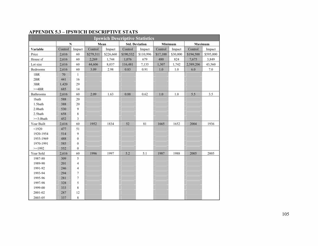
APPENDIX 5.3 – IPSWICH DESCRIPTIVE STATS Ipswich Descriptive Statistics
N Mean Std. Deviation Minimum MaximumVariable Control Impact Control Impact Control Impact Control Impact Control Impact Price 2,616 60 $279,311 $226,660 $190,532 $110,996 $17,100 $30,000 $194,500 $595,000 House sf 2,616 60 2,269 1,744 1,076 679 480 824 7,675 3,849 Lot size 2,616 60 44,606 8,037 116,481 7,135 1,307 1,742 2,589,206 43,560 Bedrooms 2,616 60 3.09 2.98 0.83 0.91 1.0 1.0 6.0 7.0 1BR 70 1 2BR 441 16 3BR 1,420 29 >=4BR 685 14 Bathrooms 2,616 60 2.09 1.63 0.88 0.62 1.0 1.0 5.5 3.5 1bath 588 20 1.5bath 388 20 2.0bath 530 9 2.5bath 658 8 >=3.0bath 452 3 Year Built 2,616 60 1952 1834 52 81 1665 1652 2004 1936 <1920 477 51 1920-1954 514 9 1955-1969 488 0 1970-1991 585 0 >=1992 552 0 Year Sold 2,616 60 1996 1997 5.2 5.1 1987 1988 2005 2005 1987-88 309 5 1989-90 201 4 1991-92 246 4 1993-94 294 7 1995-96 281 7 1997-98 328 5 1999-00 333 8 2001-02 287 12 2003-05 337 8
105
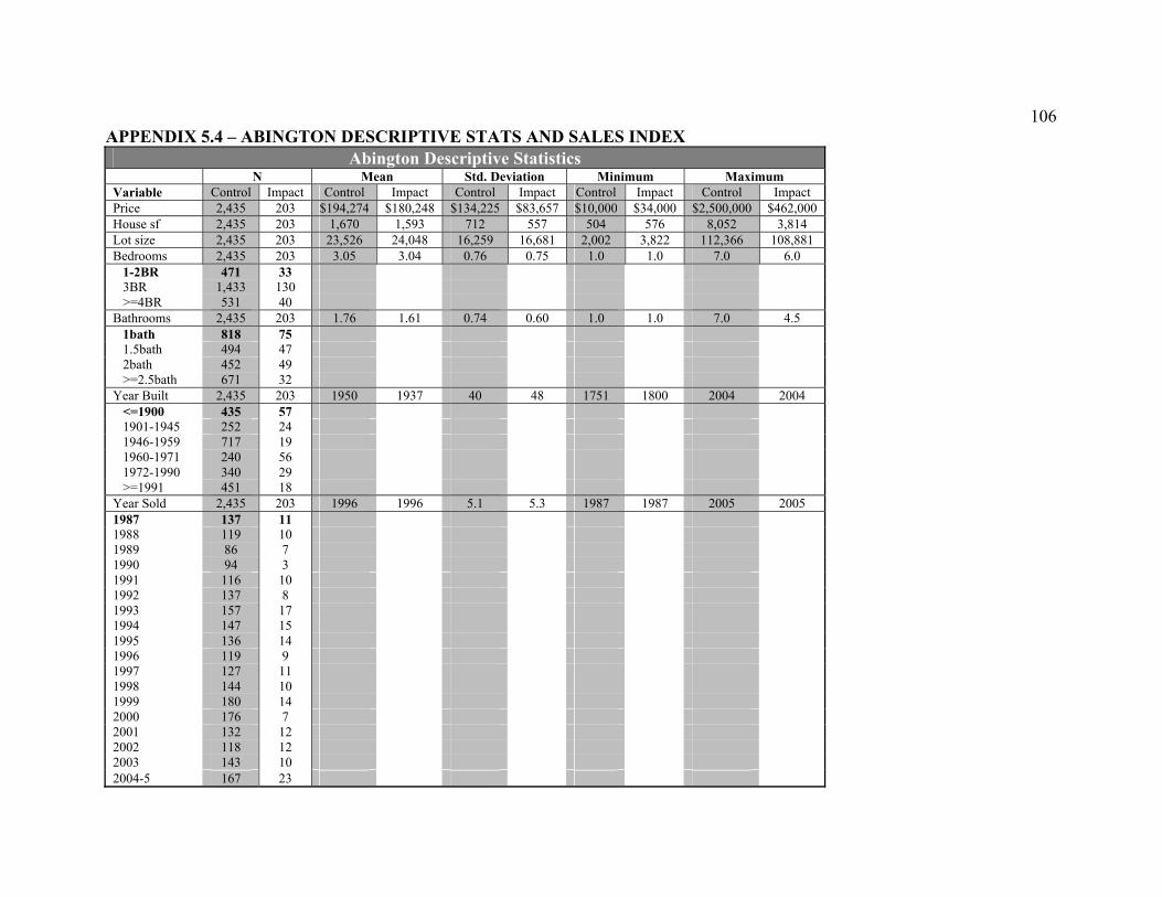
106 APPENDIX 5.4 – ABINGTON DESCRIPTIVE STATS AND SALES INDEX
Abington Descriptive Statistics N Mean Std. Deviation Minimum MaximumVariable Control Impact Control Impact Control Impact Control Impact Control Impact Price 2,435 203 $194,274 $180,248 $134,225 $83,657 $10,000 $34,000 $2,500,000 $462,000 House sf 2,435 203 1,670 1,593 712 557 504 576 8,052 3,814 Lot size 2,435 203 23,526 24,048 16,259 16,681 2,002 3,822 112,366 108,881 Bedrooms 2,435 203 3.05 3.04 0.76 0.75 1.0 1.0 7.0 6.0 1-2BR 471 33 3BR 1,433 130 >=4BR 531 40 Bathrooms 2,435 203 1.76 1.61 0.74 0.60 1.0 1.0 7.0 4.5 1bath 818 75 1.5bath 494 47 2bath 452 49 >=2.5bath 671 32 Year Built 2,435 203 1950 1937 40 48 1751 1800 2004 2004 <=1900 435 57 1901-1945 252 24 1946-1959 717 19 1960-1971 240 56 1972-1990 340 29 >=1991 451 18 Year Sold 2,435 203 1996 1996 5.1 5.3 1987 1987 2005 2005 1987 137 11 1988 119 10 1989 86 7 1990 94 3 1991 116 10 1992 137 8 1993 157 17 1994 147 15 1995 136 14 1996 119 9 1997 127 11 1998 144 10 1999 180 14 2000 176 7 2001 132 12 2002 118 12 2003 143 10 2004-5 167 23
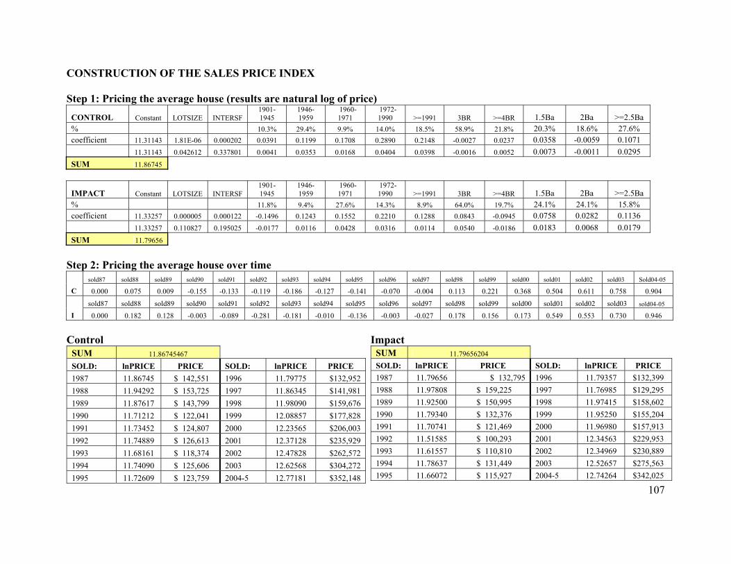
CONSTRUCTION OF THE SALES PRICE INDEX Step 1: Pricing the average house (results are natural log of price)
CONTROL Constant LOTSIZE INTERSF1901-1945
1946-1959
1960-1971
1972-1990 >=1991 3BR >=4BR 1.5Ba 2Ba >=2.5Ba
% 10.3% 29.4% 9.9% 14.0% 18.5% 58.9% 21.8% 20.3% 18.6% 27.6%coefficient 11.31143 1.81E-06 0.000202 0.0391 0.1199 0.1708 0.2890 0.2148 -0.0027 0.0237 0.0358 -0.0059 0.1071 11.31143 0.042612 0.337801 0.0041 0.0353 0.0168 0.0404 0.0398 -0.0016 0.0052 0.0073 -0.0011 0.0295SUM 11.86745
IMPACT Constant LOTSIZE INTERSF1901-1945
1946-1959
1960-1971
1972-1990 >=1991 3BR >=4BR 1.5Ba 2Ba >=2.5Ba
% 11.8% 9.4% 27.6% 14.3% 8.9% 64.0% 19.7% 24.1% 24.1% 15.8%coefficient 11.33257 0.000005 0.000122 -0.1496 0.1243 0.1552 0.2210 0.1288 0.0843 -0.0945 0.0758 0.0282 0.1136 11.33257 0.110827 0.195025 -0.0177 0.0116 0.0428 0.0316 0.0114 0.0540 -0.0186 0.0183 0.0068 0.0179SUM 11.79656
Step 2: Pricing the average house over time
sold87 sold88 sold89 sold90 sold91 sold92 sold93 sold94 sold95 sold96 sold97 sold98 sold99 sold00 sold01 sold02 sold03 Sold04-05
C 0.000 0.075 0.009 -0.155 -0.133 -0.119 -0.186 -0.127 -0.141 -0.070 -0.004 0.113 0.221 0.368 0.504 0.611 0.758 0.904
sold87 sold88 sold89 sold90 sold91 sold92 sold93 sold94 sold95 sold96 sold97 sold98 sold99 sold00 sold01 sold02 sold03 sold04-05
I 0.000 0.182 0.128 -0.003 -0.089 -0.281 -0.181 -0.010 -0.136 -0.003 -0.027 0.178 0.156 0.173 0.549 0.553 0.730 0.946
Control Impact
SUM 11.86745467
SOLD: lnPRICE PRICE SOLD: lnPRICE PRICE1987 11.86745 $ 142,551 1996 11.79775 $132,952 1988 11.94292 $ 153,725 1997 11.86345 $141,981 1989 11.87617 $ 143,799 1998 11.98090 $159,676 1990 11.71212 $ 122,041 1999 12.08857 $177,828 1991 11.73452 $ 124,807 2000 12.23565 $206,003 1992 11.74889 $ 126,613 2001 12.37128 $235,929 1993 11.68161 $ 118,374 2002 12.47828 $262,572 1994 11.74090 $ 125,606 2003 12.62568 $304,272 1995 11.72609 $ 123,759 2004-5 12.77181 $352,148
SUM 11.79656204
SOLD: lnPRICE PRICE SOLD: lnPRICE PRICE1987 11.79656 $ 132,795 1996 11.79357 $132,399 1988 11.97808 $ 159,225 1997 11.76985 $129,295 1989 11.92500 $ 150,995 1998 11.97415 $158,602 1990 11.79340 $ 132,376 1999 11.95250 $155,204 1991 11.70741 $ 121,469 2000 11.96980 $157,913 1992 11.51585 $ 100,293 2001 12.34563 $229,953 1993 11.61557 $ 110,810 2002 12.34969 $230,889 1994 11.78637 $ 131,449 2003 12.52657 $275,563 1995 11.66072 $ 115,927 2004-5 12.74264 $342,025
107

108 APPENDIX 5.5 – CONCORD DESCRIPTIVE STATS AND SALES INDEX
Concord Descriptive Statistics N Mean Std. Deviation Minimum MaximumVariable Control Impact Control Impact Control Impact Control Impact Control Impact Price 3,360 100 $522,791 $430,802 $428,048 $274,996 $10,398 $106,000 $6,025,000 $1,800,000House sf 3,360 100 2,603 2,314 1,364 1,530 321 1,076 14,286 9,276 Lot size 3,360 100 47,814 39,004 74,206 56,677 1,742 5,227 1,241,024 290,545 Bedrooms 3,360 100 3.76 3.50 0.91 0.84 1.0 2.0 8.0 6.0 1-2BR 192 5 3BR 1,120 53 4BR 1,434 33 >=5BR 614 9 Bathrooms 3,360 100 2.79 2.19 1.33 1.10 1.0 1.0 9.5 6.5 1bath 258 13 1.5-2.0bath 947 45 2.5bath 1,015 26 3.0-4.0bath 514 10 >=4.5bath 626 6 Year Built 3,360 100 1946 1934 44 46 1659 1720 2004 1999 <=1900 510 11 1901-1945 487 40 1946-1954 487 21 1955-1964 540 9 1965-1974 581 9 1975-1984 277 3 >=1985 478 7 Year Sold 3,360 100 1996 1996 5.0 4.9 1987 1987 2005 2005 1987-88 317 11 1989-90 296 8 1991-92 418 6 1993-94 416 13 1995-96 415 10 1997-98 428 20 1999-00 419 11 2001-02 312 13 2003-05 339 8
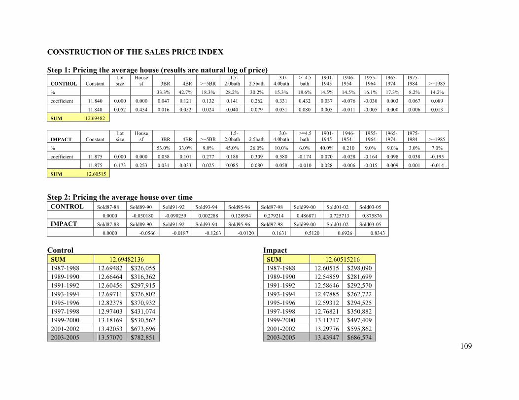
CONSTRUCTION OF THE SALES PRICE INDEX Step 1: Pricing the average house (results are natural log of price)
CONTROL Constant Lot size
House sf 3BR 4BR
>=5BR
1.5-2.0bath
2.5bath
3.0-4.0bath
>=4.5 bath
1901-1945
1946-1954
1955-1964
1965-1974
1975-1984
>=1985
% 33.3% 42.7% 18.3% 28.2% 30.2% 15.3% 18.6% 14.5% 14.5% 16.1% 17.3% 8.2% 14.2%
coefficient 11.840 0.000 0.000 0.047 0.121 0.132 0.141 0.262 0.331 0.432 0.037 -0.076 -0.030 0.003 0.067 0.089
11.840 0.052 0.454 0.016 0.052 0.024 0.040 0.079 0.051 0.080 0.005 -0.011 -0.005 0.000 0.006 0.013
SUM 12.69482
IMPACT Constant Lot size
House sf 3BR 4BR
>=5BR
1.5-2.0bath
2.5bath
3.0-4.0bath
>=4.5 bath
1901-1945
1946-1954
1955-1964
1965-1974
1975-1984 >=1985
% 53.0% 33.0% 9.0% 45.0% 26.0% 10.0% 6.0% 40.0% 0.210 9.0% 9.0% 3.0% 7.0%
coefficient 11.875 0.000 0.000 0.058 0.101 0.277 0.188 0.309 0.580 -0.174 0.070 -0.028 -0.164 0.098 0.038 -0.195
11.875 0.173 0.253 0.031 0.033 0.025 0.085 0.080 0.058 -0.010 0.028 -0.006 -0.015 0.009 0.001 -0.014
SUM 12.60515
Step 2: Pricing the average house over time
CONTROL Sold87-88 Sold89-90 Sold91-92 Sold93-94 Sold95-96 Sold97-98 Sold99-00 Sold01-02 Sold03-05 0.0000 -0.030180 -0.090259 0.002288 0.128954 0.279214 0.486871 0.725713 0.875876IMPACT Sold87-88 Sold89-90 Sold91-92 Sold93-94 Sold95-96 Sold97-98 Sold99-00 Sold01-02 Sold03-05 0.0000 -0.0566 -0.0187 -0.1263 -0.0120 0.1631 0.5120 0.6926 0.8343
Control
SUM 12.69482136 1987-1988 12.69482 $326,0551989-1990 12.66464 $316,3621991-1992 12.60456 $297,9151993-1994 12.69711 $326,8021995-1996 12.82378 $370,9321997-1998 12.97403 $431,0741999-2000 13.18169 $530,5622001-2002 13.42053 $673,6962003-2005 13.57070 $782,851
Impact SUM 12.60515216 1987-1988 12.60515 $298,0901989-1990 12.54859 $281,6991991-1992 12.58646 $292,5701993-1994 12.47885 $262,7221995-1996 12.59312 $294,5251997-1998 12.76821 $350,8821999-2000 13.11717 $497,4092001-2002 13.29776 $595,8622003-2005 13.43947 $686,574
109
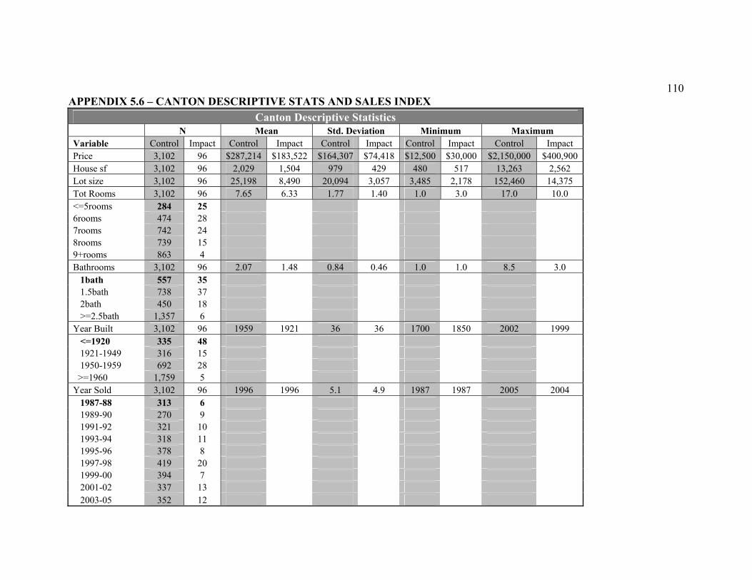
110
APPENDIX 5.6 – CANTON DESCRIPTIVE STATS AND SALES INDEX Canton Descriptive Statistics
N Mean Std. Deviation Minimum MaximumVariable Control Impact Control Impact Control Impact Control Impact Control Impact Price 3,102 96 $287,214 $183,522 $164,307 $74,418 $12,500 $30,000 $2,150,000 $400,900 House sf 3,102 96 2,029 1,504 979 429 480 517 13,263 2,562 Lot size 3,102 96 25,198 8,490 20,094 3,057 3,485 2,178 152,460 14,375 Tot Rooms 3,102 96 7.65 6.33 1.77 1.40 1.0 3.0 17.0 10.0 <=5rooms 284 25 6rooms 474 28 7rooms 742 24 8rooms 739 15 9+rooms 863 4 Bathrooms 3,102 96 2.07 1.48 0.84 0.46 1.0 1.0 8.5 3.0 1bath 557 35 1.5bath 738 37 2bath 450 18 >=2.5bath 1,357 6 Year Built 3,102 96 1959 1921 36 36 1700 1850 2002 1999 <=1920 335 48 1921-1949 316 15 1950-1959 692 28 >=1960 1,759 5 Year Sold 3,102 96 1996 1996 5.1 4.9 1987 1987 2005 2004 1987-88 313 6 1989-90 270 9 1991-92 321 10 1993-94 318 11 1995-96 378 8 1997-98 419 20 1999-00 394 7 2001-02 337 13 2003-05 352 12
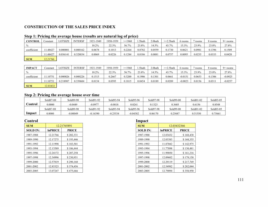
CONSTRUCTION OF THE SALES PRICE INDEX Step 1: Pricing the average house (results are natural log of price)
CONTROL Constant LOTSIZE INTERSF 1921-1949 1950-1959 >=1960 1.5bath 2.0bath >=2.5bath 6 rooms 7 rooms 8 rooms 9+ rooms % 10.2% 22.3% 56.7% 23.8% 14.5% 43.7% 15.3% 23.9% 23.8% 27.8% coefficient 11.48427 0.000001 0.000162 0.0678 0.1013 0.2264 0.0782 0.0559 0.1730 0.0621 0.0981 0.1396 0.1509
11.48427 0.036141 0.328834 0.0069 0.0226 0.1284 0.0186 0.0081 0.0757 0.0095 0.0235 0.0333 0.0420
SUM 12.21766
IMPACT Constant LOTSIZE INTERSF 1921-1949 1950-1959 >=1960 1.5bath 2.0bath >=2.5bath 6 rooms 7 rooms 8 rooms 9+ rooms % 10.2% 22.3% 56.7% 23.8% 14.5% 43.7% 15.3% 23.9% 23.8% 27.8% coefficient 11.10751 0.000026 0.000226 0.1515 0.2667 0.3200 0.1906 0.1301 0.0661 -0.0151 0.0653 0.1306 -0.0925
11.10751 0.218987 0.339604 0.0154 0.0595 0.1815 0.0454 0.0189 0.0289 -0.0023 0.0156 0.0311 -0.0257
SUM 12.03432
Step 2: Pricing the average house over time
Sold87-88 Sold89-90 Sold91-92 Sold93-94 Sold95-96 Sold97-98 Sold99-00 Sold01-02 Sold03-05Control 0.0000 -0.0449 -0.0977 -0.0818 0.0241 0.1323 0.3605 0.6156 0.8548
Sold87-88 Sold89-90 Sold91-92 Sold93-94 Sold95-96 Sold97-98 Sold99-00 Sold01-02 Sold03-05Impact 0.0000 -0.00049 -0.16390 -0.25534 -0.04382 0.06170 0.25687 0.51550 0.75661
Control Impact
SUM 12.21765891 SOLD IN: lnPRICE PRICE 1987-1988 12.21766 $ 202,331
1989-1990 12.17275 $ 193,446
1991-1992 12.11998 $ 183,501
1993-1994 12.13589 $ 186,444
1995-1996 12.24172 $ 207,258
1997-1998 12.34996 $ 230,951
1999-2000 12.57819 $ 290,160
2001-2002 12.83323 $ 374,456
2003-2005 13.07247 $ 475,666
SUM 12.03432366 SOLD IN: lnPRICE PRICE 1987-1988 12.03432 $ 168,438
1989-1990 12.03383 $ 168,355
1991-1992 11.87042 $ 142,975
1993-1994 11.77898 $ 130,481
1995-1996 11.99050 $ 161,216
1997-1998 12.09602 $ 179,158
1999-2000 12.29119 $ 217,769
2001-2002 12.54982 $ 282,044
2003-2005 12.79094 $ 358,950
111

112
SELECTED BIBLIOGRAPHY Massachusetts Housing Market Citizens Housing and Planning Association, “The Greater Boston Housing Report Card 2002,” http://www.chapa.org/completedraft.pdf Citizens Housing and Planning Association, “The Greater Boston Housing Report Card 2003,” http://www.chapa.org/HousingRCard2003.pdf Massachusetts Department of Housing and Community Development, “Draft FY2005 - 2009 Consolidated Plan and FY2005 Action Plan, Housing Market Analysis,” http://www.mass.gov/dhcd/Temp/05/05-09plan/06.pdf The Homevoter Hypothesis William A. Fischel, The Homevoter Hypothesis, Harvard University Press, Cambridge, Massachusetts, 2005. William A. Fischel (2004), An Economic History of Zoning and a Cure for Its Exclusionary Effects, Urban Studies, Volume 41, Number 2, 317-340. William A. Fischel (1999), Zoning and Land Use Regulation, http://encyclo.findlaw.com/2200book.pdf. Chapters 40B and 40R American Planning Association, Massachusetts Chapter, “Summary of M.G.L. Chapter 40R,” 2004, http://www.massapa.org/pdf/article_smartgrowthzoning.pdf Citizens Housing and Planning Association, 40B Overview, http://www.chapa.org/chapter40b.html Citizens Housing and Planning Association, “The Record on 40B,” June, 2003, http://www.chapa.org/TheRecordon40B.pdf Massachusetts Department of Housing and Community Development, Overview of The Massachusetts Comprehensive Permit Law, http://www.mass.gov/dhcd/ToolKit/ch40Bgl.htm
113
Studies on Externalities and House Prices Paul M. Cummings with John D. Landis (1993), Relationships between Affordable Housing Developments and Neighboring Property Values, Working Paper 599, Institute of Urban and Regional Development, University of California at Berkeley. Lance Freeman and Hilary Botein (2002), Subsidized Housing and Neighborhood Impacts: A Theoretical Discussion and Review of the Evidence, Journal of Planning Literature, 16(3), 359-378. George C. Galster (2002), A Review of Existing Research on the Effects of Federally Assisted Housing Programs on Neighboring Residential Property Values, Report to the National Association of Realtors. Edward G. Goetz, Hin Kin Lam, and Anne Heitlinger (1996), There goes the Neighborhood? The Impact of Subsidized Multi-Family Housing on Urban Neighborhoods, Center for Urban and Regional Affairs, University of Minnesota. Richard K. Green, Stephen Malpezzi and Kiat-Yong Seah (2002), Low Income Housing Tax Credit Housing Developments and Property Values, The Center for Urban Land Economics Research, The University of Wisconsin, Wisconsin-Madison CULER Working Papers, 1-10. Chang-Moo Lee, Dennis P. Culhane, and Susan M. Wachter, The Differential Impacts of Federally Assisted Housing Programs on Nearby Property Values: A Philadelphia Case Study, Housing Policy Debate, 10(1), 75-93. Robert F. Lyons and Scott Loveridge (1993), An Hedonic Estimation of the Effect of Federally Subsidized Housing on Nearby Residential Property Values, Department of Agricultural and Applied Economics, University of Minnesota, Staff Paper, 93-6. Maxfield Research and the Family Housing Fund (2000), A Study of the Relationship between Affordable Family Rental Housing and Home Values in the Twin Cities, http://www.fhfund.org/Research/Maxfield-Exec%20Summary.pdf David J. Ritchay and Zoë R. Weinrobe (2004), Fear and Loathing in Massachusetts: Chapter 40B, Community Opposition, and Residential Property Value, Masters Thesis, Department of Urban Studies and Planning, Massachusetts Institute of Technology Joyce Siegel, with Grier Partnership (2001), The House Next Door, Innovative Housing Institute, http://www.inhousing.org/housenex.htm Strategic Economics (2004), Memorandum: Impacts of New Attached Housing on Surrounding Single Family Home Values, http://www.ci.mtnview.ca.us/citynews/pdf/mm_092004_Community_Property_Values_Report.pdf
114

Weinstein, Emily R. (2002), Irrational market : facts and fiction behind affordable housing in the San Francisco Bay Area, Masters Thesis, Department of Urban Studies and Planning, Massachusetts Institute of Technology. Case Studies and Town Profiles Affordable Housing Online, http://www.affordablehousingonline.com Community Profiles, Massachusetts Department of Housing and Community Development, http://www.mass.gov/dhcd/iprofile/ O’Connell, James, C., Ahead or Behind the Curve?: Compact Mixed-Use Development in Suburban Boston, August, 2004, http://www.massapa.org/pdf/report_aheadbehindcurve.pdf O’Connell, James, C., Ahead or Behind the Curve?: Compact Mixed-Use Development in Suburban Boston (Figures and Photos), http://www.lincolninst.edu/pubs/dl/878_OConnell_WEB_photos_only.pdf Aerial Photos and Images Community Photo Search, Executive Office of Environmental Affairs, http://commpres.env.state.ma.us/search/photo_search.asp OLIVER – The MassGIS Online Data Viewer, MassGIS, http://maps.massgis.state.ma.us/massgis_viewer/index.htm Yahoo! Maps, http://maps.yahoo.com Quantitative Methodology and Hedonic Price Modeling Kees Jan van Garderen and Chandra Shah (2002), The interpretation of dummy variables in semilogarithmic equations in the presence of estimation uncertainty, UVA Econometrics, Discussion Paper: 2002/10, Universiteit Van Amsterdam. R. Halvorsen and R. Palmquist (1980), The interpretation of dummy variables in semilogarithmuc equations, American Economic Review, 70, 474-475. Stephen Malpezzi (2002), Hedonic Pricing Models: A Selective and Applied Review, Prepared for: Housing Economics: Essays in Honor of Duncan Maclennan, The Center for Urban Land Economics Research, The University of Wisconsin.
115

116
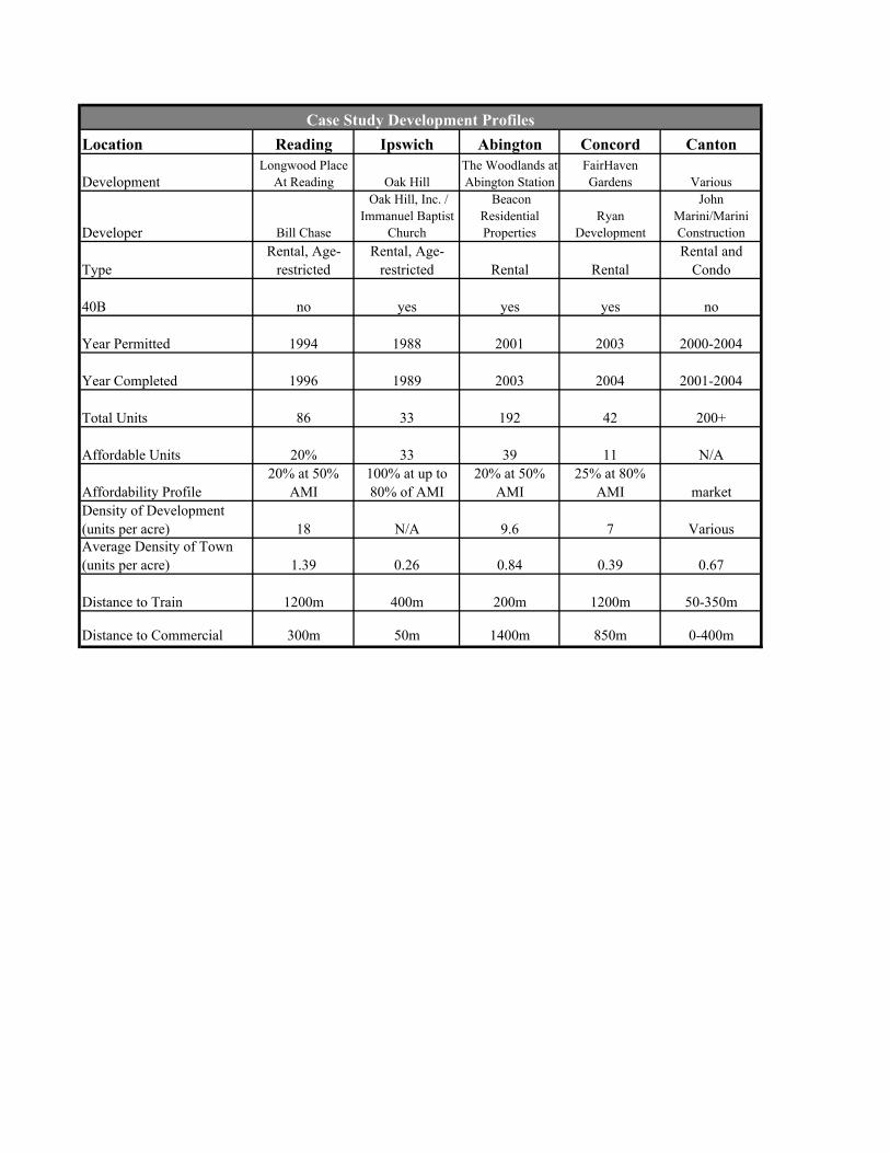
Case Study Development ProfilesLocation Reading Ipswich Abington Concord Canton
DevelopmentLongwood Place
At Reading Oak Hill The Woodlands atAbington Station
FairHaven Gardens Various
Developer Bill Chase
Oak Hill, Inc. / Immanuel Baptist
Church
Beacon Residential Properties
Ryan Development
John Marini/Marini Construction
TypeRental, Age-
restrictedRental, Age-
restricted Rental RentalRental and
Condo
40B no yes yes yes no
Year Permitted 1994 1988 2001 2003 2000-2004
Year Completed 1996 1989 2003 2004 2001-2004
Total Units 86 33 192 42 200+
Affordable Units 20% 33 39 11 N/A
Affordability Profile20% at 50%
AMI100% at up to 80% of AMI
20% at 50% AMI
25% at 80% AMI market
Density of Development (units per acre) 18 N/A 9.6 7 VariousAverage Density of Town (units per acre) 1.39 0.26 0.84 0.39 0.67
Distance to Train 1200m 400m 200m 1200m 50-350m
Distance to Commercial 300m 50m 1400m 850m 0-400m
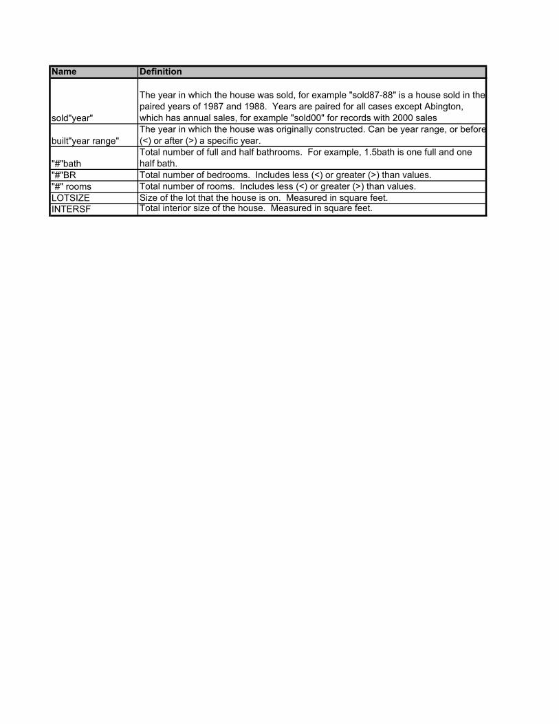
Name Definition
sold"year"
The year in which the house was sold, for example "sold87-88" is a house sold in the paired years of 1987 and 1988. Years are paired for all cases except Abington, which has annual sales, for example "sold00" for records with 2000 sales
built"year range"The year in which the house was originally constructed. Can be year range, or before(<) or after (>) a specific year.
"#"bathTotal number of full and half bathrooms. For example, 1.5bath is one full and one half bath.
"#"BR Total number of bedrooms. Includes less (<) or greater (>) than values."#" rooms Total number of rooms. Includes less (<) or greater (>) than values.LOTSIZE Size of the lot that the house is on. Measured in square feet.INTERSF Total interior size of the house. Measured in square feet.
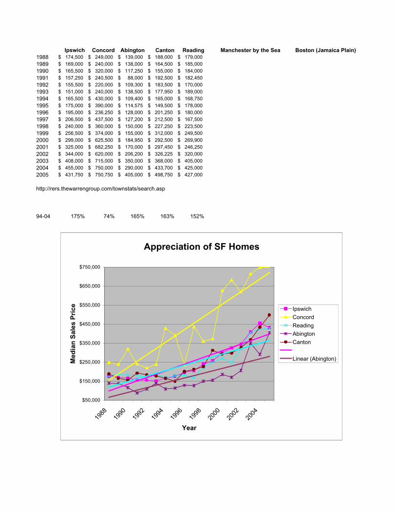
Ipswich Concord Abington Canton Reading Manchester by the Sea Boston (Jamaica Plain)1988 $ 174,500 $ 249,000 $ 139,000 $ 188,000 $ 179,000 1989 $ 169,000 $ 240,000 $ 138,000 $ 164,500 $ 185,000 1990 $ 165,500 $ 320,000 $ 117,250 $ 155,000 $ 184,000 1991 $ 157,250 $ 240,500 $ 88,000 $ 192,500 $ 182,450 1992 $ 155,500 $ 220,000 $ 109,300 $ 183,500 $ 170,000 1993 $ 151,000 $ 240,000 $ 138,500 $ 177,950 $ 189,000 1994 $ 165,500 $ 430,000 $ 109,400 $ 165,000 $ 168,750 1995 $ 175,000 $ 390,000 $ 114,575 $ 149,500 $ 178,000 1996 $ 195,000 $ 236,250 $ 128,000 $ 201,250 $ 180,000 1997 $ 206,500 $ 437,500 $ 127,200 $ 212,500 $ 167,500 1998 $ 240,000 $ 360,000 $ 150,000 $ 227,250 $ 223,500 1999 $ 256,500 $ 374,000 $ 155,000 $ 312,000 $ 249,500 2000 $ 299,000 $ 625,500 $ 184,950 $ 292,500 $ 269,900 2001 $ 325,000 $ 682,250 $ 170,000 $ 297,450 $ 246,250 2002 $ 344,000 $ 620,000 $ 206,200 $ 326,225 $ 320,000 2003 $ 408,000 $ 715,000 $ 350,000 $ 368,000 $ 405,000 2004 $ 455,000 $ 750,000 $ 290,000 $ 433,700 $ 425,000 2005 $ 431,750 $ 750,750 $ 405,000 $ 498,750 $ 427,000
http://rers.thewarrengroup.com/townstats/search.asp
94-04 175% 74% 165% 163% 152%
Appreciation of SF Homes
$50,000
$150,000
$250,000
$350,000
$450,000
$550,000
$650,000
$750,000
1988
1990
1992
1994
1996
1998
2000
2002
2004
Year
Med
ian
Sale
s Pr
ice Ipswich
ConcordReadingAbingtonCanton
Linear (Abington)
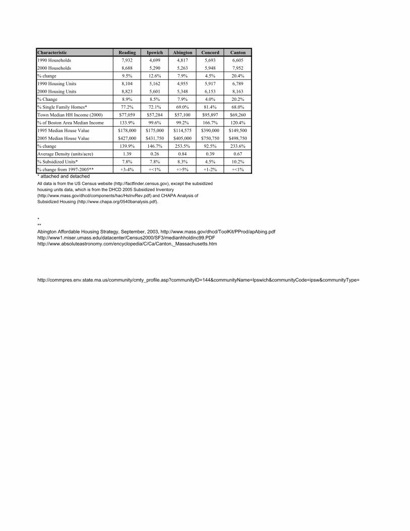
Characteristic Reading Ipswich Abington Concord Canton1990 Households 7,932 4,699 4,817 5,693 6,6052000 Households 8,688 5,290 5,263 5,948 7,952% change 9.5% 12.6% 7.9% 4.5% 20.4%1990 Housing Units 8,104 5,162 4,955 5,917 6,7892000 Housing Units 8,823 5,601 5,348 6,153 8,163% Change 8.9% 8.5% 7.9% 4.0% 20.2%% Single Family Homes* 77.2% 72.1% 69.0% 81.4% 68.0%Town Median HH Income (2000) $77,059 $57,284 $57,100 $95,897 $69,260% of Boston Area Median Income 133.9% 99.6% 99.2% 166.7% 120.4%1995 Median House Value $178,000 $175,000 $114,575 $390,000 $149,5002005 Median House Value $427,000 $431,750 $405,000 $750,750 $498,750% change 139.9% 146.7% 253.5% 92.5% 233.6%Average Density (units/acre) 1.39 0.26 0.84 0.39 0.67% Subsidized Units* 7.8% 7.8% 8.3% 4.5% 10.2%% change from 1997-2005** +3-4% +<1% +>5% +1-2% +<1%* attached and detachedAll data is from the US Census website (http://factfinder.census.gov), except the subsidizedhousing units data, which is from the DHCD 2005 Subsidized Inventory (http://www.mass.gov/dhcd/components/hac/HsInvRev.pdf) and CHAPA Analysis of Subsidized Housing (http://www.chapa.org/0540banalysis.pdf).
* ** Abington Affordable Housing Strategy, September, 2003, http://www.mass.gov/dhcd/ToolKit/PProd/apAbing.pdfhttp://www1.miser.umass.edu/datacenter/Census2000/SF3/medianhholdinc99.PDFhttp://www.absoluteastronomy.com/encyclopedia/C/Ca/Canton,_Massachusetts.htm
http://commpres.env.state.ma.us/community/cmty_profile.asp?communityID=144&communityName=Ipswich&communityCode=ipsw&communityType=
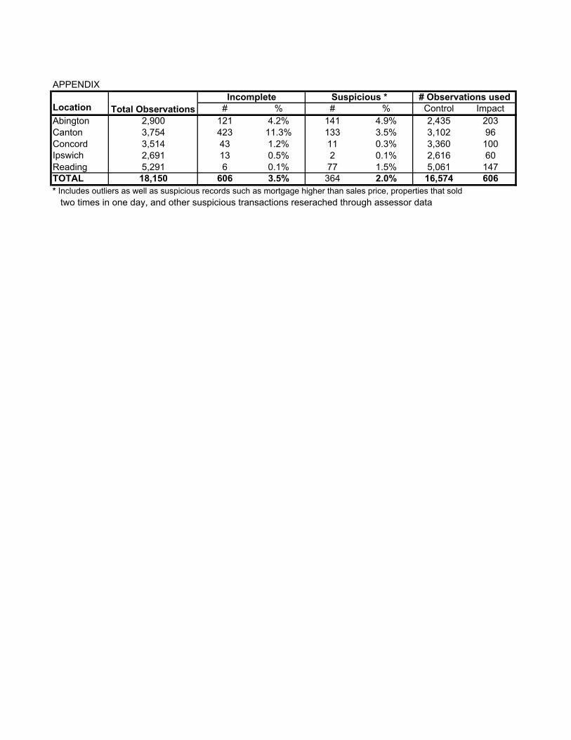
APPENDIX
Location # % # % Control ImpactAbington 2,900 121 4.2% 141 4.9% 2,435 203Canton 3,754 423 11.3% 133 3.5% 3,102 96Concord 3,514 43 1.2% 11 0.3% 3,360 100Ipswich 2,691 13 0.5% 2 0.1% 2,616 60Reading 5,291 6 0.1% 77 1.5% 5,061 147TOTAL 18,150 606 3.5% 364 2.0% 16,574 606* Includes outliers as well as suspicious records such as mortgage higher than sales price, properties that sold two times in one day, and other suspicious transactions reserached through assessor data
Incomplete Suspicious * # Observations usedTotal Observations
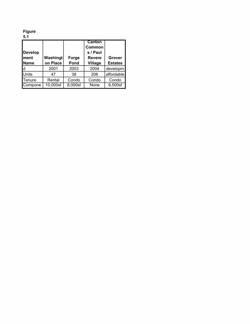
Figure 5.1
Development Name
Washington Place
Forge Pond
Canton Commons / Paul Revere Village
Grover Estates
d 2001 2003 2004 developmUnits 47 38 206 affordableTenure Rental Condo Condo CondoCompone 10,000sf 8,000sf None 6,500sf

Location Reading Ipswich Abington Concord Canton
DevelopmentLongwood Place
At Reading Oak Hill The Woodlands at Abington Station
FairHaven Gardens Various
Developer Bill Chase
Oak Hill, Inc. / Immanuel Baptist
Church
Beacon Residential Properties
Ryan Development
John Marini/Marini Construction
TypeRental, Age-
restrictedRental, Age-
restricted Rental RentalRental and
Condo
40B no yes yes yes no
Year Permitted 1994 1988 2001 2003 2000-2004
Year Completed 1996 1989 2003 2004 2001-2004
Total Units 86 33 192 42 200+
Affordable Units 20% 33 39 11 N/A
Affordability Profile20% at 50%
AMI100% at up to 80% of AMI
20% at 50% AMI
25% at 80% AMI market
Density of Development (units per acre) 18 N/A 9.6 7 VariousAverage Density of Town (units per acre) 1.39 0.26 0.84 0.39 0.67
Distance to Train 1200m 400m 200m 1200m 50-350m
Distance to Commercial 300m 50m 1400m 850m 0-400m
Case Study Development Profiles