The Impact of Monetary Policy Shocks on … Impact of Monetary Policy Shocks on Commodity Prices∗ Alessio Anzuini,a Marco J. Lombardi,b and Patrizio Paganoa aBanca d’Italia bBank

The Impact of Monetary Policy Shocks onCommodity Prices∗

Alessio Anzuini,a Marco J. Lombardi,b and Patrizio Paganoa

aBanca d’ItaliabBank for International Settlements

Global monetary conditions are often cited as a driver ofcommodity prices. This paper investigates the empirical rela-tionship between U.S. monetary policy and commodity pricesby means of a standard VAR system, commonly used in analyz-ing the effects of monetary policy shocks. The results suggestthat expansionary U.S. monetary policy shocks drive up thebroad commodity price index and all of its components. Whilethese effects are significant, they do not, however, appear tobe overwhelmingly large.

JEL Codes: E31, E40, C32.

1. Introduction

Commodity price developments have been one of the major sourcesof concern for policymakers in recent years. After surging rapidly tounprecedented levels in the course of 2008, commodity prices fellabruptly in the wake of the financial crisis and global economicdownturn. Since the beginning of 2009, however, they first stabi-lized and then resumed an upward path, characterized by relativelyhigh volatility. As commodity prices in general—and the price ofoil in particular—are an important component of a consumer priceindex (CPI), their evolution and the driving forces behind them areclearly crucial for the conduct of monetary policy (Svensson 2005).

∗We gratefully acknowledge useful comments received from the editor andtwo anonymous referees. We also thank Lutz Kilian, Ron Alquist, and all sem-inar participants at the Bank of Canada, the Bank of Chile, and the Bank ofEngland. Views expressed in this paper are solely those of the authors andshould not be attributed to the Bank of Italy or the BIS. Author e-mails:[email protected]; [email protected] (corresponding author);[email protected].

119

120 International Journal of Central Banking September 2013

A wide strand of literature has examined the impact of commod-ity prices—oil in particular—on macroeconomic variables (see, e.g.,Kilian 2008 for a survey), but less attention has been devoted to theother direction of causality, i.e., the impact of monetary conditionson oil and other commodity prices. In this paper we focus on the lat-ter relationship to analyze how far an expansionary monetary policyshock can drive up commodity prices and through which channel.

While supply and demand factors can generally explain the bulkof the fluctuations in commodity prices, other forces may at timesplay a role (Hamilton 2009). Kilian (2009) and Alquist and Kilian(2010) highlight the relevance, in the behavior of oil prices, of pre-cautionary demand shocks, which increase current demand for oilthrough increased uncertainty about future oil supply shortfalls.1

Since the seminal contribution of Frankel (1984), monetary condi-tions and interest rates have attracted attention as possible drivingfactors of commodity prices. Frankel (1986) extends Dornbusch’stheory of exchange rate overshooting to the case of commodities and,using no-arbitrage conditions, derives a theoretical link between oilprices and interest rates. Barsky and Kilian (2002, 2004) show thatmonetary policy stance is a good predictor of commodity prices. Inparticular, Barsky and Kilian (2002) also suggest that the oil priceincreases of the 1970s could have been caused, at least in part, bymonetary conditions.2

Most of the empirical literature devoted to the assessment ofthe relationship between monetary policy and commodity prices hasfocused on the U.S. interest rate as an indicator of monetary pol-icy stance (Frankel 2007; Frankel and Rose 2010). However, interestrates may not fully represent the impact of a monetary policy shockand, more importantly, their movements can reflect the endogenousresponse of monetary policy to general developments in the econ-omy. For instance, Bernanke, Gertler, and Watson (1997), using aVAR framework, suggest that positive shocks to oil prices inducea monetary policy response which can amplify the contractionary

1Anzuini, Pagano, and Pisani (2007) show that such oil shocks contributedsignificantly to U.S. recessions.

2Nakov and Pescatori (2010) argue, in line with Kilian (2009), that oil pricesshould be treated endogenously in dynamic stochastic general equilibrium mod-els as well. Hence, Gillman and Nakov (2009) find that nominal oil prices reactproportionally to nominal interest rate shocks.

Vol. 9 No. 3 The Impact of Monetary Policy Shocks 121

effects of the oil price shock itself. Kilian and Lewis (2011), how-ever, report no evidence of a systematic Federal Reserve reaction tooil shocks after 1987.

During the commodity price surge of 2008, some commentatorssuggested that loose monetary policy and persistently low interestrates could have, at least in part, fueled the price hike (Hamilton2009). If this is so, then it is important to understand whether andto what extent the massive monetary policy easing now taking placewill sow the seeds of another surge in commodity prices. In thispaper, we do not work with a plain analysis of co-movement betweencommodity prices and interest rates; instead we identify a monetarypolicy shock in a VAR system for the U.S. economy and then assessits impact on commodity prices. This allows us not only to exam-ine the impact of monetary policy net of other interaction channelsbut also to avoid employing indicators of global monetary condi-tions that are inherently difficult to measure. More specifically, weuse a standard identification scheme for the monetary policy shock(Kim 1999) and then project each of the commodity prices on thisshock in order to single out the responses of the different pricesto the same monetary policy shock. We find empirical evidence ofa significant impact of monetary policy on commodity prices. Inparticular, a 100-basis-point expansionary monetary policy shockdrives up moderately the broad commodity price index and all of itsmajor components, with the increase ranging from 4 to 7 percent atthe peak. Although the methodology is very different, our approachis similar in spirit to that of Frankel and Hardouvelis (1985), whoinvestigated the impact of money-supply announcements on com-modity prices; the main difference is that we work with an identifiedmonetary policy shock in a VAR system.

We assess the robustness of the results by repeating the exer-cise using several different identification strategies of the monetarypolicy shock that are commonly used in the literature. In partic-ular, remaining in a VAR context, we also use a Choleski identi-fication strategy similar to that proposed by Boivin and Giannoni(2006) and the one based on sign restrictions in the spirit of Canovaand De Nicolo (2002) and Uhlig (2005). We also analyze the effecton commodity prices of both the monetary policy shocks identifiedaccording to Kuttner (2001) and to Romer and Romer (2004). Weconclude that, overall, all these strategies lead to similar conclusions.


The decomposition of the forecast-error variance suggests thatmonetary policy shocks help predict fluctuations in commodityprices, even though they are not the major source of them. Regard-ing the commodity price surge between 2003 and 2008, historicaldecomposition shows that accumulated past monetary policy shockscontributed to the increase in the broad commodity price index andin its main components, but they explain just a small part of thepeak in the price of oil and nothing of that in food prices.

Finally, we shed some light on the channels through which mon-etary policy shocks may affect commodity prices as suggested byFrankel (2007), focusing on the case of oil. In particular, we showthat the positive impact on oil prices of a monetary policy looseningcan be ascribed to incentives to stock accumulation and to disincen-tives to immediate production; the link with financial flows is muchless evident.

The paper is organized as follows. In section 1 we evaluate theimpact of monetary policy shocks on the commodity price indexand on its major components, describing first the data and the VARframework. Next, we present an impulse response analysis. In section2 we evaluate the extent of the role of monetary policy shocks inexplaining commodity price fluctuations. In section 3 we focus on thetransmission channels through which monetary policy may directlyaffect commodity prices. The last section contains some concludingremarks.

2. Monetary Shocks and Commodity Prices

2.1 Data and Model Details

To gauge the quantitative effect of monetary policy shocks oncommodity prices, we estimate a VAR for the United States, thelargest oil-consuming economy in the world. Our data set consistsof monthly variables from January 1970 to December 2008.3 Admit-tedly, this covers a very long time span during which policy shiftsmay have occurred, as documented also by Barsky and Kilian (2004).

3We decided to shorten the endpoint of the sample at the end of 2008, as thefederal funds rate was then decreased to almost zero and that lower bound mightimpair the identification scheme.


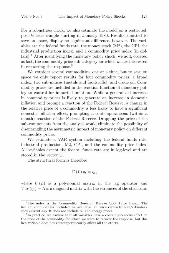
For a robustness check, we also estimate the model on a restricted,post-Volcker sample starting in January 1980. Results, omitted tosave on space, display no significant difference, however. The vari-ables are the federal funds rate, the money stock (M2), the CPI, theindustrial production index, and a commodity price index (in dol-lars).4 After identifying the monetary policy shock, we add, orderedas last, the commodity price sub-category for which we are interestedin recovering the response.5

We consider several commodities, one at a time, but to save onspace we only report results for four commodity prices: a broadindex, two sub-indices (metals and foodstuffs), and crude oil. Com-modity prices are included in the reaction function of monetary pol-icy to control for imported inflation. While a generalized increasein commodity prices is likely to generate an increase in domesticinflation and prompt a reaction of the Federal Reserve, a change inthe relative price of a commodity is less likely to have a significantdomestic inflation effect, prompting a contemporaneous (within amonth) reaction of the Federal Reserve. Dropping the price of thesub-components from the analysis would eliminate the possibility ofdisentangling the asymmetric impact of monetary policy on differentcommodity prices.

We estimate a VAR system including the federal funds rate,industrial production, M2, CPI, and the commodity price index.All variables except the federal funds rate are in log-level and arestored in the vector yt.

The structural form is therefore

C (L) yt = ηt,

where C (L) is a polynomial matrix in the lag operator andV ar (ηt) = Λ is a diagonal matrix with the variances of the structural

4The index is the Commodity Research Bureau Spot Price Index. Thelist of commodities included is available at www.crbtrader.com/crbindex/spot current.asp. It does not include oil and energy prices.

5In practice, we assume that all variables have a contemporaneous effect onthe price of the commodity for which we want to recover the response, but thislast variable does not contemporaneously affect all the others.


shocks as elements. We estimate (ignoring predetermined variables)the reduced form:

yt = A (L) yt−1 + εt,

where A (L) is a polynomial matrix in the lag operator andV ar (εt) = Σ and ηt = C0εt and therefore Σ = C−1

0 ΛC−1′0 .

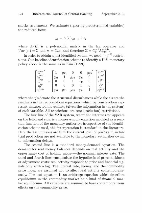
In order to obtain a just identified system, we need n(n−1)2 restric-

tions. Our baseline identification scheme to identify a U.S. monetarypolicy shock is the same as in Kim (1999):

⎡⎢⎢⎢⎢⎣

ηmst

ηmdt

ηcpit

ηipt

ηcomt

⎤⎥⎥⎥⎥⎦ =

⎡⎢⎢⎢⎢⎣

1 g12 0 0 g15g21 1 g23 g24 00 0 1 g34 00 0 0 1 0

g51 g52 g53 g54 1

⎤⎥⎥⎥⎥⎦

⎡⎢⎢⎢⎢⎣

εmst

εmdt

εcpit

εipt

εcomt

⎤⎥⎥⎥⎥⎦ ,

where the η’s denote the structural disturbances while the ε’s are theresiduals in the reduced-form equations, which by construction rep-resent unexpected movements (given the information in the system)of each variable. All restrictions are zero (exclusion) restrictions.

The first line of the VAR system, where the interest rate appearson the left-hand side, is a money-supply equation modeled as a reac-tion function of the monetary authority; irrespective of the identifi-cation scheme used, this interpretation is standard in the literature.Here the assumptions are that the current level of prices and indus-trial production are not available to the monetary authorities owingto information delays.

The second line is a standard money-demand equation. Thedemand for real money balances depends on real activity and theopportunity cost of holding money—the nominal interest rate. Thethird and fourth lines encapsulate the hypothesis of price stickinessor adjustment costs: real activity responds to price and financial sig-nals only with a lag. The interest rate, money, and the commodityprice index are assumed not to affect real activity contemporane-ously. The last equation is an arbitrage equation which describesequilibrium in the commodity market as a kind of financial mar-ket equilibrium. All variables are assumed to have contemporaneouseffects on the commodity price.


As is common in the oil literature (e.g., Kilian 2009), we selecttwelve lags: with monthly data our lag structure captures one year ofdynamics, which appears to be sufficient to eliminate autocorrelationof residuals.6

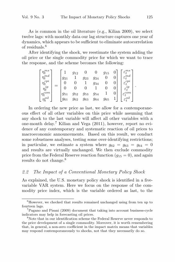
After identifying the shock, we reestimate the system adding theoil price or the single commodity price for which we want to tracethe response, and the scheme becomes the following:

⎡⎢⎢⎢⎢⎢⎢⎣

ηmst

ηmdt

ηcpit

ηipt

ηcomt

ηoilt

⎤⎥⎥⎥⎥⎥⎥⎦

=

⎡⎢⎢⎢⎢⎢⎢⎣

1 g12 0 0 g15 0g21 1 g23 g24 0 00 0 1 g34 0 00 0 0 1 0 0

g51 g52 g53 g54 1 0g61 g62 g63 g64 g65 1

⎤⎥⎥⎥⎥⎥⎥⎦

⎡⎢⎢⎢⎢⎢⎢⎣

εmst

εmdt

εcpit

εipt

εcomt

εoilt

⎤⎥⎥⎥⎥⎥⎥⎦

.

In ordering the new price as last, we allow for a contemporane-ous effect of all other variables on this price while assuming thatany shock to the last variable will affect all other variables with aone-month delay.7 Kilian and Vega (2011), however, report no evi-dence of any contemporary and systematic reaction of oil prices tomacroeconomic announcements. Based on this result, we conductsome robustness analyses, testing some over-identifying restrictions;in particular, we estimate a system where g62 = g63 = g64 = 0and results are virtually unchanged. We then exclude commodityprice from the Federal Reserve reaction function (g15 = 0), and againresults do not change.8

2.2 The Impact of a Conventional Monetary Policy Shock

As explained, the U.S. monetary policy shock is identified in a five-variable VAR system. Here we focus on the response of the com-modity price index, which is the variable ordered as last, to the

6However, we checked that results remained unchanged using from ten up tofourteen lags.

7Pagano and Pisani (2009) document that taking into account business-cycleindicators may help in forecasting oil prices.

8Note that in our identification scheme the Federal Reserve never responds tothe price development of a single commodity. Moreover, it is worth rememberingthat, in general, a non-zero coefficient in the impact matrix means that variablesmay respond contemporaneously to shocks, not that they necessarily do so.


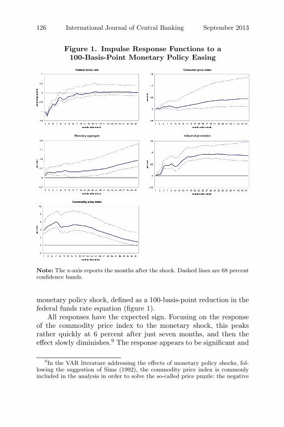
Figure 1. Impulse Response Functions to a100-Basis-Point Monetary Policy Easing

Note: The x-axis reports the months after the shock. Dashed lines are 68 percentconfidence bands.

monetary policy shock, defined as a 100-basis-point reduction in thefederal funds rate equation (figure 1).

All responses have the expected sign. Focusing on the responseof the commodity price index to the monetary shock, this peaksrather quickly at 6 percent after just seven months, and then theeffect slowly diminishes.9 The response appears to be significant and

9In the VAR literature addressing the effects of monetary policy shocks, fol-lowing the suggestion of Sims (1992), the commodity price index is commonlyincluded in the analysis in order to solve the so-called price puzzle: the negative


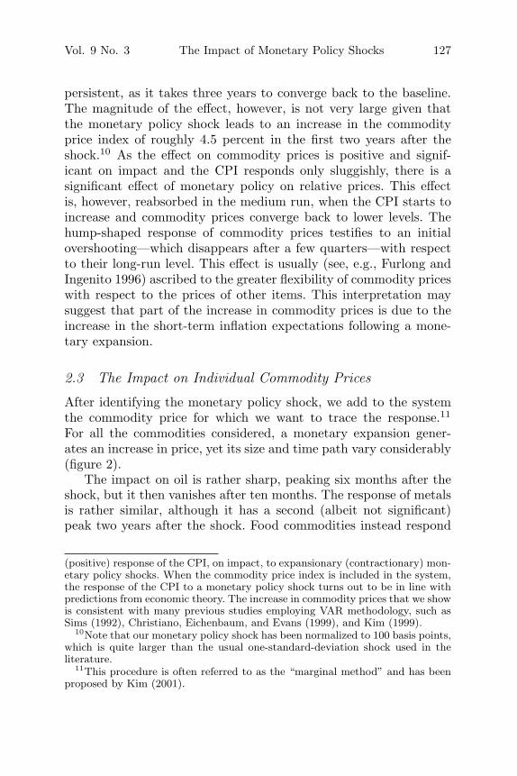
persistent, as it takes three years to converge back to the baseline.The magnitude of the effect, however, is not very large given thatthe monetary policy shock leads to an increase in the commodityprice index of roughly 4.5 percent in the first two years after theshock.10 As the effect on commodity prices is positive and signif-icant on impact and the CPI responds only sluggishly, there is asignificant effect of monetary policy on relative prices. This effectis, however, reabsorbed in the medium run, when the CPI starts toincrease and commodity prices converge back to lower levels. Thehump-shaped response of commodity prices testifies to an initialovershooting—which disappears after a few quarters—with respectto their long-run level. This effect is usually (see, e.g., Furlong andIngenito 1996) ascribed to the greater flexibility of commodity priceswith respect to the prices of other items. This interpretation maysuggest that part of the increase in commodity prices is due to theincrease in the short-term inflation expectations following a mone-tary expansion.

2.3 The Impact on Individual Commodity Prices

After identifying the monetary policy shock, we add to the systemthe commodity price for which we want to trace the response.11

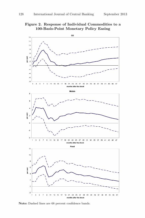
For all the commodities considered, a monetary expansion gener-ates an increase in price, yet its size and time path vary considerably(figure 2).

The impact on oil is rather sharp, peaking six months after theshock, but it then vanishes after ten months. The response of metalsis rather similar, although it has a second (albeit not significant)peak two years after the shock. Food commodities instead respond

(positive) response of the CPI, on impact, to expansionary (contractionary) mon-etary policy shocks. When the commodity price index is included in the system,the response of the CPI to a monetary policy shock turns out to be in line withpredictions from economic theory. The increase in commodity prices that we showis consistent with many previous studies employing VAR methodology, such asSims (1992), Christiano, Eichenbaum, and Evans (1999), and Kim (1999).

10Note that our monetary policy shock has been normalized to 100 basis points,which is quite larger than the usual one-standard-deviation shock used in theliterature.

11This procedure is often referred to as the “marginal method” and has beenproposed by Kim (2001).


Figure 2. Response of Individual Commodities to a100-Basis-Point Monetary Policy Easing

Note: Dashed lines are 68 percent confidence bands.


in a more persistent fashion, as the effects remain significant up tothree years after the shock has occurred. In all cases the size of theresponse is quite moderate, ranging between 4 and 7 percent at thepeak.

While the increase in the prices of oil and of other commodi-ties involved in the industrial process is intuitive, explaining theincrease in food price is trickier. One explanation, put forward inTimilsina, Mevel, and Shrestha (2011), is that an increase in oilprices would reduce the global food supply through direct impactsas well as through the diversion of food commodities and croplandtowards the production of biofuels.

2.4 Robustness

Results presented above rest on the identifying assumptions of themonetary policy shock. Admittedly, the scheme we have employed(Kim 1999) is not the only one possible, and we chose it on thegrounds of its close connection with our setup, as well as for itssimplicity and widespread use in the literature. In this section weexamine to what extent our results remain valid when using differentidentification schemes for the monetary policy shock. The literatureon monetary policy shocks is vast and we do not aim to be exhaus-tive. Rather, we concentrate on four schemes that somehow stemfrom different approaches to the issue and which are very popularin the applied literature.

The first alternative shock we consider follows an approach sim-ilar to that of Christiano, Eichenbaum, and Evans (1996, 1999) andis based on a simple VAR with Choleski identification featuring (inorder) output, CPI, commodity prices, and the federal funds rate.12

This approach has become very popular in the recent years, due toits simplicity.

The second alternative identification scheme is based on signrestrictions. Following Faust (1998), Canova and De Nicolo (2002),

12Christiano, Eichenbaum, and Evans (1996) work with quarterly variablesand use GDP as a measure of output and the GDP deflator as a measure ofinflation. Given our monthly setup, we had to replace this with, respectively,industrial production and CPI. However, this does not seem to affect the validityof the identification scheme. Correspondingly, as they employ four lags, we selecttwelve. Note also that this scheme has more recently been used by Boivin andGiannoni (2006).


and Uhlig (2005), we impose sign restrictions directly on impulseresponses; i.e., after an expansionary monetary policy shock, theinterest rate falls while money, output, and prices rise.13 As we focuson the response of commodity prices, no restriction is imposed onthis variable. The response of the single sub-component of the com-modity price index is then obtained (as before) by simply addingthe new variable to the old system without any further restriction.The actual implementation of this scheme is obtained through a QRdecomposition following Rubio-Ramırez, Waggoner, and Zha (2010).We will use this identification strategy only to assess the robust-ness of the response of commodity prices (and sub-components) toa monetary policy shock. While in our view sign restrictions are auseful tool in SVAR analysis, we acknowledge that they have beenthe subject of some criticism, given that all percentiles of the dis-tribution in this case are computed across different rotations, whichcorrespond to different models (Fry and Pagan 2007). To circumventthis critique, we could extract a monetary policy shock by selectingan arbitrary rotation or averaging across shocks generated by dif-ferent rotations; however, as a certain degree of arbitrariness wouldbe involved in this process, we decided not to use the shock seriesimplied by this identification procedure in the robustness analysis ofthe transmission channel of the next section.

We then move to other identification schemes not based on aVAR: our third alternative relies instead on financial market infor-mation. Kuttner (2001) proposes gauging a monetary policy shockby subtracting from the actual change in the federal funds rate itsexpectation, i.e., computing the difference between federal fundsfutures immediately before and after the decision of the FederalOpen Market Committee (FOMC). The idea is that many of themonetary policy decisions (and often the size of the change) areexpected and therefore cannot be labeled “shocks.” The remainingmonetary policy “surprises” that agents face should therefore pro-duce stronger effects. This series of monetary policy shocks is avail-able since 1989, when the futures market for the federal funds ratewas established at the Chicago Board of Trade. To determine how

13Such responses are constrained for three periods. The lags included in theVAR are twelve.


commodity prices respond to monetary shocks, we simply regressthe log change in the commodity price index on a constant, its ownlagged values, and lagged values of the policy measure. The laggedvalues of the shock series are included to capture the direct impactof shocks on commodity price changes, and the lagged values of com-modity price changes are included to control for the normal dynamicsof the commodity price index.14

The last alternative monetary policy shock series we consider isthat derived by Romer and Romer (2004). This scheme combinesnarrative accounts of each FOMC meeting included in the minuteswith the Federal Reserve’s internal forecasts of inflation and realactivity (the “Greenbook” forecasts) to purge the intended fundsrate of monetary policy actions taken in response to informationabout future economic developments. The resulting series of mon-etary shocks should show changes in the funds rate not made inresponse to information about future economic developments. Unfor-tunately, the series is not very up-to-date, as it is available only fromJanuary 1969 to December 1996.15

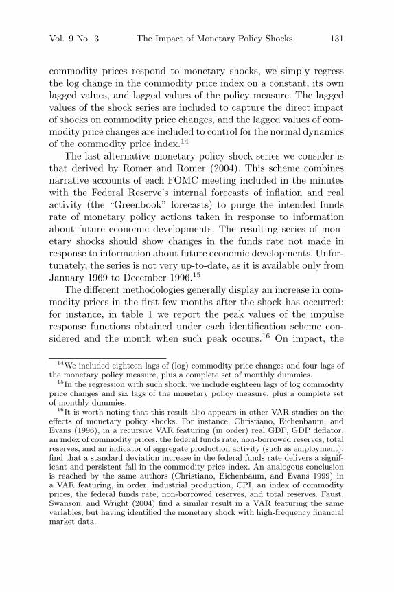
The different methodologies generally display an increase in com-modity prices in the first few months after the shock has occurred:for instance, in table 1 we report the peak values of the impulseresponse functions obtained under each identification scheme con-sidered and the month when such peak occurs.16 On impact, the

14We included eighteen lags of (log) commodity price changes and four lags ofthe monetary policy measure, plus a complete set of monthly dummies.

15In the regression with such shock, we include eighteen lags of log commodityprice changes and six lags of the monetary policy measure, plus a complete setof monthly dummies.

16It is worth noting that this result also appears in other VAR studies on theeffects of monetary policy shocks. For instance, Christiano, Eichenbaum, andEvans (1996), in a recursive VAR featuring (in order) real GDP, GDP deflator,an index of commodity prices, the federal funds rate, non-borrowed reserves, totalreserves, and an indicator of aggregate production activity (such as employment),find that a standard deviation increase in the federal funds rate delivers a signif-icant and persistent fall in the commodity price index. An analogous conclusionis reached by the same authors (Christiano, Eichenbaum, and Evans 1999) ina VAR featuring, in order, industrial production, CPI, an index of commodityprices, the federal funds rate, non-borrowed reserves, and total reserves. Faust,Swanson, and Wright (2004) find a similar result in a VAR featuring the samevariables, but having identified the monetary shock with high-frequency financialmarket data.


Table 1. Peak Responses of Various Commodity Pricesafter a Differently Identified Monetary Policy Shock

Sign Romer &Kim Choleski Restrictions Romer Kuttner

Commodity 6.0 [6] 0.7 [6] 3.4 [6] 2.7 [15] 4.0 [3]Index

Oil 7.7 [6] 2.1 [5] 14.4 [5] 3.0 [4] 7.1 [5]Metals 4.3 [2] 0.2 [2] 5.0 [6] 2.0 [13] 8.6 [3]Food 6.6 [6] 2.4 [5] 5.7 [3] 8.0 [4] 6.2 [3]

Notes: Maximum percentage changes of commodity prices after a –100-basis-pointsmonetary policy shock identified with different methodologies. For Kim, Choleski,and sign restrictions: median responses. In square brackets: month of the maximumresponse.

responses obtained with the monetary shock a la Kuttner (2001)are the most similar to those with Kim’s identification, but they arealso rather short-lived; the other responses are less pronounced butconsiderably more persistent.17 Overall, the robustness exercise sup-ports the above conclusion that commodity prices increase after anexpansionary monetary policy shock but that the size of the effectis generally moderate.

3. Monetary Policy and Commodity Prices Fluctuations

3.1 Forecast-Error-Variance Decomposition

Given the significant effect of monetary shocks, one may wonderhow large is their relative contribution to overall commodity pricefluctuations. This question can be tackled by means of a forecast-error-variance decomposition, which measures the percentage shareof the forecast-error variance due to a specific shock at a specifictime horizon.

17Scrimgeour (2010) estimates the effect of a monetary policy surprise oncommodity prices with an instrumental-variables method, finding a very similarresult: a 100-basis-point surprise increase in interest rates leads to an immediate5 percent decline in commodity prices.


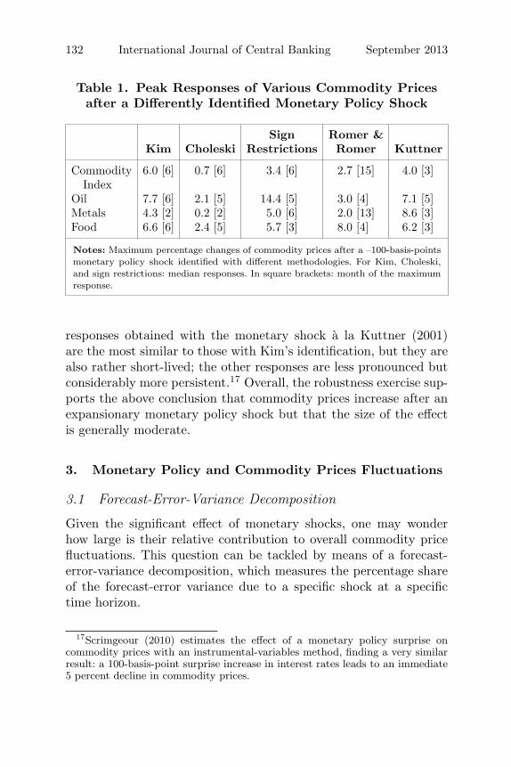
Figure 3. Forecast-Error-Variance Decomposition

Note: Dashed lines are 68 percent confidence bands.

In figure 3 we report the forecast-error-variance decomposition ofthe commodity price index and individual commodities with respectto the monetary shocks. The horizons at which forecast errors arecalculated are indicated on the x-axis. The median percentage of thevariance of the commodity index hovers around 20 percent, whereascontributions to oil and metals prices are, respectively, around 6and 8 percent. Food commodities appear to have responded morestrongly to monetary policy shocks, posting a variance contributionof around 20 percent.

Overall, we may conclude that monetary policy shocks help pre-dict commodity price movements but are not the main source offluctuations in prices. This result is in line with that of Barskyand Kilian (2002), Frankel (2007), and Frankel and Rose (2010),who find, at best, mixed evidence on the impact of interest rates oncommodity prices.

3.2 Historical Decomposition

In this section we address the following question: to what extenthave monetary policy shocks contributed to the recent movements


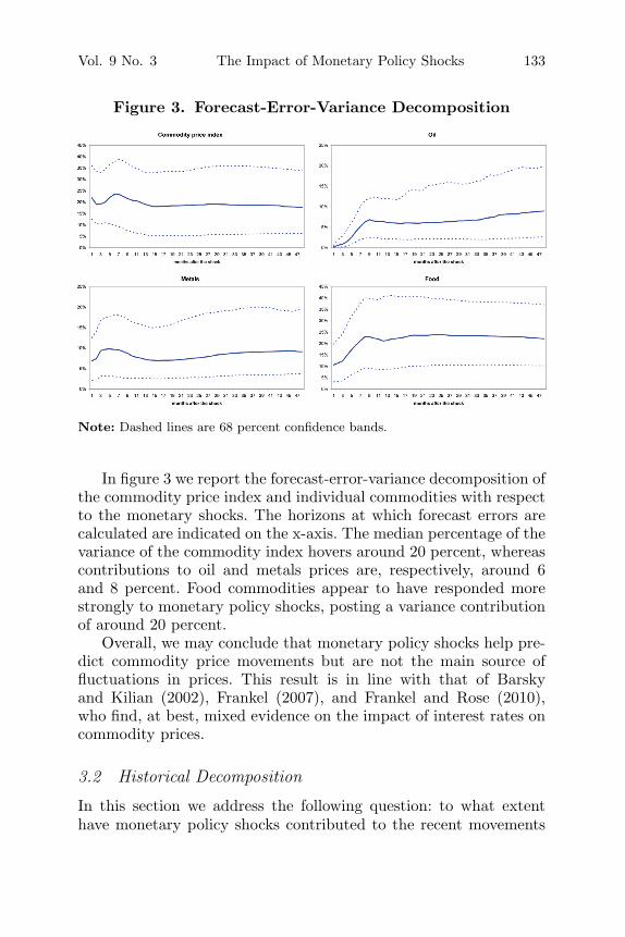
Figure 4. Historical Decomposition

in commodity prices? Similarly to Kilian (2009), we calculate thecumulative contribution of the monetary shock to the price ofthe different commodities based on a historical decomposition ofthe data. These estimates are, naturally, subject to considerablesampling uncertainty, so they should be considered to be onlysuggestions.

The exhibits presented in figure 4 focus on the period betweenJanuary 2003 and July 2008, when all the commodities under exam-ination recorded a run-up. The role of accumulated past monetarypolicy shocks (the dashed line) appears generally limited, althoughdifferentiated across commodities. In particular, the non-systematiccomponent of monetary policy appears to have contributed to theincrease in commodity prices above the baseline since early 2006,but it has not contributed to their peak at mid-2008.

Focusing on the case of oil, the contribution of monetary policyshocks to the increase in oil prices in 2006 and 2007 is non-trivial,but it fades after early 2008 and is quite limited when oil pricespeak. Viewing this result through the lens of the direct transmissionchannels—which will be analyzed in the next section—it is strikingthat in 2007–08, despite the reduction in interest rates, in the United


States oil inventories were actually depleted.18 Since OPEC, crudeoil production did not increase much and, in particular, did not keeppace with oil demand: in mid-2008, when oil prices reached recordhighs, OPEC excess capacity was down to 1 million barrels a day.Whether the sensitivity of these channels to monetary policy shockshas changed over time is beyond the scope of this work, but it mayprove an interesting route for future investigation.

4. Transmission Channels

Having found a significant impact of monetary policy shocks oncommodity prices, we still do not know through which channel theeffect takes place. Barsky and Kilian (2002, 2004) argue that thechannels through which monetary policy exerts its impact on com-modity prices are (expectations of) stronger inflation and economicgrowth. There are, however, a number of other channels, related tothe opportunity cost of investing in real assets, according to whichan expansionary monetary policy can cause an increase in com-modity prices. Frankel (2007) summarizes them as follows: (i) lowinterest rates tend to reduce the opportunity cost of carrying inven-tories, increasing the demand for commodities (inventory channel);(ii) on the supply side, lower rates create an incentive not to extractexhaustible commodities today, as the cost of holding inventories“in the ground” also decreases (supply channel); and (iii) for a givenexpected price path, a decrease in interest rates reduces the carryingcost of speculative positions, making it easier to bet on assets suchas commodities; under certain conditions, this will put upward pres-sure on futures prices and, by arbitrage, also on spot prices (financialchannel).

In what follows we investigate the relevance of these alternativechannels in the case of oil. The reasons for this choice are twofold:on the one hand, oil is by far the most important commodity for theglobal economy, and its macroeconomic impacts have been studiedextensively; on the other hand, comprehensive data is available oninventories and production, which is not the case for other commodi-ties. In particular, we check whether the monetary policy shock a la

18Plante and Yucel (2011) show that floating storage in oil tankers also declinedthroughout the summer of 2008.


Kim (1999) derived in section 1 helps to explain the fluctuations inoil inventories, oil supply, and speculative activity in futures markets.

4.1 Monetary Policy Shock and Transmission Channels

Let us start by looking at the inventory channel. Holding oil inven-tories has a cost not only in terms of the fee due to the owner ofthe storage facilities but also because of the opportunity cost ofusing money to buy oil which goes into storage and is not immedi-ately burnt instead of investing the amount needed at the risk-freerate. Of course, that cost will be lower in an environment of lowinterest rates. Hence, loose monetary policy may generate incen-tives to accumulate inventories, thereby raising the demand for oilas well as its price. To check whether this channel appears to be atwork, we regress a measure of crude oil inventories on the monetarypolicy shock, as well as the respective lags. The data on oil invento-ries refers to U.S. industry stocks of crude oil, collected by the U.S.Energy Information Administration, and covers the period from Jan-uary 1970 to December 2008; data is expressed in month-on-monthgrowth rates.19 This is admittedly only a partial representation ofthe status of global oil inventories, which also comprise stocks heldin other countries as well as floating storage. Yet no reliable data isavailable for non-OECD inventories and floating storage, and datafor inventories held in OECD countries is available only at quarterlyfrequency and for a shorter time span.

An environment of loose monetary policy will not only haveimpact on the fundamentals of the oil market via the incentives toaccumulate inventories. Oil producers will also have fewer incentivesto pump enough oil to satisfy growing demand. The reason is thatthe opportunity cost of leaving oil in the ground with the expec-tation of selling it later for a higher price will be lower. Therefore,producers facing the decision whether to extract oil immediately andinvest the revenues at the current (low) interest rate or, rather, toleave oil in the ground may indeed prefer to postpone extraction. Tocheck whether this is indeed the case, we regress a measure of worldoil supply on the monetary policy shock, as well as the respective

19We deliberately exclude government stocks since in their case accumulationdepends on considerations other than interest rates.


lags. The data on oil supply refers to world production of crude oilas measured by the International Energy Agency and is from Feb-ruary 1984 to December 2008; data is expressed in month-on-monthgrowth rates.

Finally, loose monetary policy could also affect physical oilprices via the futures market channel. Low interest rates imply thatinvestors will have stronger incentives to chase risky assets (such ascommodities) in search of higher returns. In addition, the opportu-nity cost of carrying speculative positions in the oil futures marketis reduced. This may encourage speculators to take long positions inthe futures market, thereby exerting upward pressure on the futurescurve. In the case of frictions to arbitrage opportunities, this pressurecould eventually transmit to physical spot prices.20 To assess theimportance of this channel, we regress a measure of speculative activ-ity in oil futures markets on the monetary policy shock, as well as therespective lags. Unfortunately, measuring speculative activity in thecrude oil futures market is a daunting task. The U.S. Commission forFutures Trading in Commodities (CFTC) collects and disseminatesweekly data on the positions held by non-commercial agents in WTIcrude oil futures contracts traded on the NYMEX; data is avail-able since January 1996. A measure of speculative activity widelyemployed in the literature is the so-called non-commercial net longposition, i.e., the difference between the number of long and shortpositions held by agents not related to physical oil.21 The rationale isthat a positive net positioning suggests that non-commercial agents,i.e., speculators, are mostly bullish about oil price prospects. In prac-tical terms, we regress the month-on-month percentage changes in

20For a detailed overview of how the linkage between futures and spot pricesworks and how frictions may hamper it, including some empirical results, seeLombardi and Van Robays (2011).

21There are a number of caveats relating to the measurement of speculativeactivity with such an indicator. First of all, the distinction between commer-cial and non-commercial agents is somewhat arbitrary and does not imply thatonly non-commercials can act as speculators: for example, shouldn’t an airlinebetting on oil price increases also be labeled a speculator? And why should apension fund taking a long position in energy futures to diversify its portfolioand hedge against inflation be labeled a speculator? Second, index funds, i.e.,financial instruments that replicate oil price developments, are managed by swapdealers and hence fall in the commercial category. Finally, data is incomplete, asit covers only regulated markets.


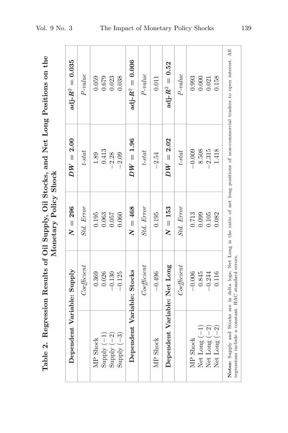
oil supply and oil stocks and the ratio of net long positions in futuresto open interest on their lags and on the monetary policy shock.22

In table 2 we report the coefficient of the monetary shock as wellas the lagged coefficient of the dependent variable selected usingthe Schwarz information criterion. As we used a generated regres-sor (the monetary shock), we report Newey-West (HAC) standarderrors. Results highlight that all variables are somewhat sensitive tothe monetary policy shock. The signs of all coefficients are in linewith the theory: a tightening of the monetary policy stance (i.e., apositive shock) produces an increase in oil production (as producersfind it more convenient to extract oil today and invest their revenuesat higher rates), a decrease in oil inventories (as the opportunity costof holding inventories rises), and a decrease in speculative positions(as investors face a higher opportunity cost). However, the effectof the monetary shock on speculative positions is statistically notsignificant. It is also interesting to note that lagged values of themonetary policy shock always appear to be non-significant and werediscarded in the model-selection process.

4.2 Robustness

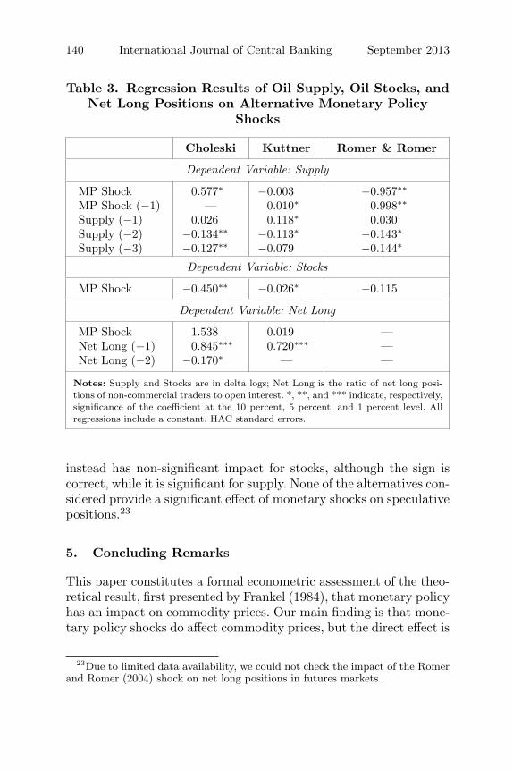
To check the robustness of our results on the transmission channel,we repeat the regression of table 2 employing different identificationschemes for the monetary policy shock as explanatory variables. Asin section 2.4, we use a very simple Choleski scheme (Boivin andGiannoni 2006), a financial-markets-based measure (Kuttner 2001),and a more narrative approach (Romer and Romer 2004).

The results of the regressions are reported in table 3. The shock ala Boivin and Giannoni (2006), being the one most closely related inits construction to that of Kim (1999), gives results that are very sim-ilar to those of table 2 and thus confirms our analysis. For the othertwo shocks, the picture is a bit more blurred. Kuttner (2001) doesgive favorable results for the impact of the monetary policy shockon stocks, while the effect on supply is significant only with a lag.The shock extracted using the Romer and Romer (2004) approach

22The series of oil stocks and, to a lesser extent, oil production present a markedpattern of seasonality, which was removed by simply regressing each series onseasonal dummies.


Tab

le2.

Reg

ress

ion

Res

ults

ofO

ilSupply

,O

ilSto

cks,

and

Net

Lon

gPos

itio

ns

onth

eM

onet

ary

Pol

icy

Shock

Dep

enden

tV

aria

ble

:Supply

N=

296

DW

=2.

00ad

j-R

2=

0.03

5

Coe

ffici

ent

Std.

Err

ort-st

atP-v

alue

MP

Shoc

k0.

369

0.19

51.

890.

059

Supp

ly(−

1)0.

026

0.06

30.

413

0.67

9Su

pply

(−2)

−0.

130

0.05

7−

2.28

0.02

3Su

pply

(−3)

−0.

125

0.06

0−

2.09

0.03

8

Dep

enden

tV

aria

ble

:Sto

cks

N=

468

DW

=1.

96ad

j-R

2=

0.00

6

Coe

ffici

ent

Std.

Err

ort-st

atP-v

alue

MP

Shoc

k−

0.49

60.

195

−2.

540.

011

Dep

enden

tV

aria

ble

:N

etLon

gN

=15

3D

W=

2.02

adj-R

2=

0.52

Coe

ffici

ent

Std.

Err

ort-st

atP-v

alue

MP

Shoc

k−

0.00

60.

713

−0.

009

0.99

3N

etLon

g(−

1)0.

845

0.09

98.

508

0.00

0N

etLon

g(−

2)−

0.24

40.

105

−2.

315

0.02

1N

etLon

g(−

2)0.

116

0.08

21.

418

0.15

8

Note

s:Supply

and

Sto

cks

are

indel

talo

gs;

Net

Lon

gis

the

rati

oof

net

long

pos

itio

ns

ofnon

-com

mer

cial

trad

ers

toop

enin

tere

st.

All

regr

essi

ons

incl

ude

aco

nst

ant.

HA

Cst

andar

der

rors

.


Table 3. Regression Results of Oil Supply, Oil Stocks, andNet Long Positions on Alternative Monetary Policy

Shocks

Choleski Kuttner Romer & Romer

Dependent Variable: Supply

MP Shock 0.577∗ −0.003 −0.957∗∗

MP Shock (−1) — 0.010∗ 0.998∗∗

Supply (−1) 0.026 0.118∗ 0.030Supply (−2) −0.134∗∗ −0.113∗ −0.143∗

Supply (−3) −0.127∗∗ −0.079 −0.144∗

Dependent Variable: Stocks

MP Shock −0.450∗∗ −0.026∗ −0.115

Dependent Variable: Net Long

MP Shock 1.538 0.019 —Net Long (−1) 0.845∗∗∗ 0.720∗∗∗ —Net Long (−2) −0.170∗ — —

Notes: Supply and Stocks are in delta logs; Net Long is the ratio of net long posi-tions of non-commercial traders to open interest. *, **, and *** indicate, respectively,significance of the coefficient at the 10 percent, 5 percent, and 1 percent level. Allregressions include a constant. HAC standard errors.

instead has non-significant impact for stocks, although the sign iscorrect, while it is significant for supply. None of the alternatives con-sidered provide a significant effect of monetary shocks on speculativepositions.23

5. Concluding Remarks

This paper constitutes a formal econometric assessment of the theo-retical result, first presented by Frankel (1984), that monetary policyhas an impact on commodity prices. Our main finding is that mone-tary policy shocks do affect commodity prices, but the direct effect is

23Due to limited data availability, we could not check the impact of the Romerand Romer (2004) shock on net long positions in futures markets.


not overwhelmingly large. With regard to oil, this conclusion is cor-roborated by the analysis of the impact of supply, inventories, andfinancial activity in futures. Notice, however, that a stronger effectof monetary policy on commodity prices may pass through the indi-rect channels of expected economic growth and inflation (Barskyand Kilian 2004).

Our findings also suggest that the extraordinary monetary pol-icy easing deployed to contrast the real effects of the financial cri-sis is likely to push commodity prices up, albeit not to a greatextent. However, we acknowledge that our identification scheme isnot designed to account for unconventional monetary policy meas-ures, so that larger effects cannot be ruled out. While this is, ofcourse, an interesting avenue of research, it would require a brand-new identification strategy for the monetary policy shock, which isbeyond the scope of this paper.

References

Alquist, R., and L. Kilian. 2010. “What Do We Learn from the Priceof Crude Oil Futures?” Journal of Applied Econometrics 25 (4):539–73.

Anzuini, A., P. Pagano, and M. Pisani. 2007. “Oil Supply News in aVAR: Information from Financial Markets.” Temi di discussioneNo. 632. Banca d’Italia.

Barsky, R. B., and L. Kilian. 2002. “Do We Really Know ThatOil Caused the Great Stagflation? A Monetary Alternative.” InNBER Macroeconomics Annual 2001, ed. B. S. Bernanke and K.Rogoff, 137–98. Cambridge, MA: MIT Press.

———. 2004. “Oil and the Macroeconomy Since the 1970s.” Journalof Economic Perspectives 18 (4): 115–34.

Bernanke, B. S., M. Gertler, and M. W. Watson. 1997. “SystematicMonetary Policy and the Effects of Oil Price Shocks.” BrookingsPapers on Economic Activity 1: 91–142.

Boivin, J., and M. P. Giannoni. 2006. “Has Monetary Policy BecomeMore Effective?” Review of Economics and Statistics 88 (3):445–62.

Canova, F., and G. De Nicolo. 2002. “Monetary Disturbances Mat-ter for Business Fluctuations in the G-7.” Journal of MonetaryEconomics 49 (6): 1121–59.


Christiano, L. J., M. Eichenbaum, and C. L. Evans. 1996. “TheEffects of Monetary Policy Shocks: Evidence from the Flow ofFunds.” Review of Economics and Statistics 78 (1): 16–34.

———. 1999. “Monetary Policy Shocks: What Have We Learnedand to What End?” In Handbook of Macroeconomics, Vol. 1A,ed. J. Taylor and M. Woodford, 65–148. Elsevier.

Faust, J. 1998. “The Robustness of Identified VAR Conclusionsabout Money.” Carnegie-Rochester Conference Series on PublicPolicy 49 (December): 207–44.

Faust, J., E. T. Swanson, and J. H. Wright. 2004. “Identifying VARSBased on High Frequency Futures Data.” Journal of MonetaryEconomics 51 (6): 1107–31.

Frankel, J. A. 1984. “Commodity Prices and Money: Lessons fromInternational Finance.” American Journal of Agricultural Eco-nomics 66 (5): 560–66.

———. 1986. “Expectations and Commodity Price Dynamics: TheOvershooting Model.” American Journal of Agricultural Eco-nomics 68 (2): 344–48.

———. 2007. “The Effect of Monetary Policy on Real CommodityPrices.” In Asset Prices and Monetary Policy, ed. J. Campbell.Chicago: University of Chicago Press.

Frankel, J. A, and G. K. Hardouvelis. 1985. “Commodity Prices,Money Surprises, and Fed Credibility.” Journal of Money, Creditand Banking 17 (4): 427–38.

Frankel, J. A., and A. K. Rose. 2010. “Determinants of Agriculturaland Mineral Commodity Prices.” In Inflation in an Era of Rel-ative Price Shocks, eds. R. Fry, C. Jones, and C. Kent. ReserveBank of Australia.

Fry, R., and A. Pagan. 2007. “Some Issues in Using Sign Restrictionsfor Identifying Structural VARs.” National Centre for Economet-ric Research Working Paper No. 14.

Furlong, F., and R. Ingenito. 1996. “Commodity Prices and Infla-tion.” Economic Review (Federal Reserve Bank of San Francisco)1996 (2): 27–47.

Gillman, M., and A. A. Nakov. 2009. “Monetary Effects on NominalOil Prices.” North American Journal of Economics and Finance20 (3): 239–54.

Hamilton, J. D. 2009. “Understanding Crude Oil Prices.” EnergyJournal 30 (2): 179–206.


Kilian, L. 2008. “The Economic Effects of Energy Price Shocks.”Journal of Economic Literature 46 (4): 871–909.

———. 2009. “Not All Oil Price Shocks Are Alike: DisentanglingDemand and Supply Shocks in the Crude Oil Market.” AmericanEconomic Review 99 (3): 1053–69.

Kilian, L., and L. Lewis. 2011. “Does the Fed Respond to Oil PriceShocks?” Economic Journal 121 (555): 1047–72.

Kilian, L., and C. Vega. 2011. “Do Energy Prices Respond to U.S.Macroeconomic News? A Test of the Hypothesis of Predeter-mined Energy Prices.” Review of Economics and Statistics 93(2): 660–71.

Kim, S. 1999. “Do Monetary Shocks Matter in the G-7 Countries?Using Common Identifying Assumptions about Monetary PolicyAcross Countries.” Journal of International Economics 48 (2):387–175.

———. 2001. “International Transmission of U.S. Monetary PolicyShocks: Evidence from VARs.” Journal of Monetary Economics48 (2): 339–72.

Kuttner, K. N. 2001. “Monetary Policy Surprises and Interest Rates:Evidence from the Fed Funds Futures Markets.” Journal of Mon-etary Economics 47 (3): 523–44.

Lombardi, M., and I. Van Robays. 2011. “Do Financial InvestorsDestabilize the Oil Price?” ECB Working Paper No. 1346.

Nakov, A. A., and A. Pescatori. 2010. “Oil and the Great Modera-tion.” Economic Journal 120 (543): 131–56.

Pagano, P., and M. Pisani. 2009. “Risk-Adjusted Forecasts of OilPrices.” The B.E. Journal of Macroeconomics 9 (1): Article 24.

Plante, M. D., and M. K. Yucel. 2011. “Did Speculation DriveOil Prices? Market Fundamentals Suggest Otherwise.” EconomicLetter (Federal Reserve Bank of Dallas) 6 (11).

Romer, C. D., and D. H. Romer. 2004. “A New Measure of Mone-tary Shocks: Derivation and Implications.” American EconomicReview 94 (4): 1055–84.

Rubio-Ramırez, J. F., D. Waggoner, and T. Zha. 2010. “StructuralVector Autoregressions: Theory of Identification and Algorithmsfor Inference.” Review of Economic Studies 77 (2): 665–96.

Scrimgeour, D. 2010. “Commodity Price Responses to MonetaryPolicy Surprises.” Working Paper No. 2010-04, Department ofEconomics, Colgate University.


Sims, C. 1992. “Interpreting the Macroeconomic Time Series Facts:The Effects of Monetary Policy.” European Economic Review 36(5): 975–1000.

Svensson, L. E. O. 2005. “Oil Prices and ECB Monetary Pol-icy.” Manuscript. Available at http://people.su.se/˜leosven/papers/ep501.pdf.

Timilsina, G. R., S. Mevel, and A. Shrestha. 2011. “World Oil Priceand Biofuels: A General Equilibrium Analysis.” World Bank Pol-icy Research Working Paper No. 5673.

Uhlig, H. 2005. “What Are the Effects of Monetary Policy on Out-put? Results from an Agnostic Identification Procedure.” Journalof Monetary Economics 52 (2): 381–419.

Documents

The Impact of Monetary Policy Shocks on … Impact of Monetary Policy Shocks on Commodity Prices∗ Alessio Anzuini,a Marco J. Lombardi,b and Patrizio Paganoa aBanca d’Italia bBank