The impact of moist singular vectors and ensemble size on predicted storm tracks for the winter storms Lothar and Martin

A. Walser1)

M. Arpagaus1)

M. Leutbecher2)

1)MeteoSwiss, Zurich

2)ECMWF, Reading, GB

Moist vs. operational singular vectorsCoutinho et al. (2004)

‚opr‘ SVs (T42L31, OT 48 h): linearized physics package with surface drag simple vertical diffusion

‚moist‘ SVs (T63L31, OT 24 h): linearized physics package includes additionally: gravity wave drag long-wave radiation deep cumulus convection large-scale condensation

Martin: Predicted storm tracks t+(42-66) < 980 hPa (1)

ensemble members: 2 tracks ▬ analysis

< 970 hPa< 960 hPa

Configuration:

• dry SVs/51 RMs

• moist SVs/51 RMs

Martin: Predicted storm tracks t+(42-66) < 980 hPa (2)

ensemble members: 12 tracks ▬ analysis

< 970 hPa< 960 hPa

Configuration:

• dry SVs/51 RMs

• moist SVs/51 RMs

moist SVs, x~10 km

Forecast storm Martin: max. wind gusts t+(30-54) (4)

Configuration:

• moist SVs/51 RMs

• moist SVs/10 RMs

Evaluation of the COSMO-LEPS forecasts for the floods in Switzerland in August 2005 and further recent results…

André Walser

MeteoSwiss, Zurich

Case study: Flood event in Switzerland in August 2005

Photos:Tages-Anzeiger

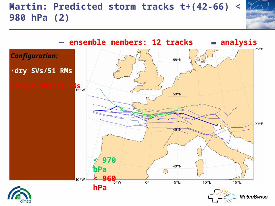
Synoptic overview: 22 August 2005

Temperature 850 hPa and geopotential 500 hPa:

2º

18º

10º

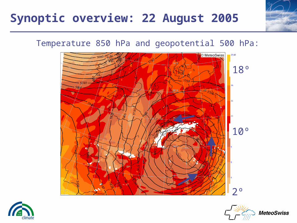
Total precipitation over 3 days (20. – 22.8.)

About 400 stations, precipitation sum locally over 300 mm!

(06 - 06 UTC)

C. Frei, MeteoSwiss

COSMO-LEPS forecast for 72h precipitation

Probability precipitation > 100mm/72h

C. Frei, MeteoSwiss

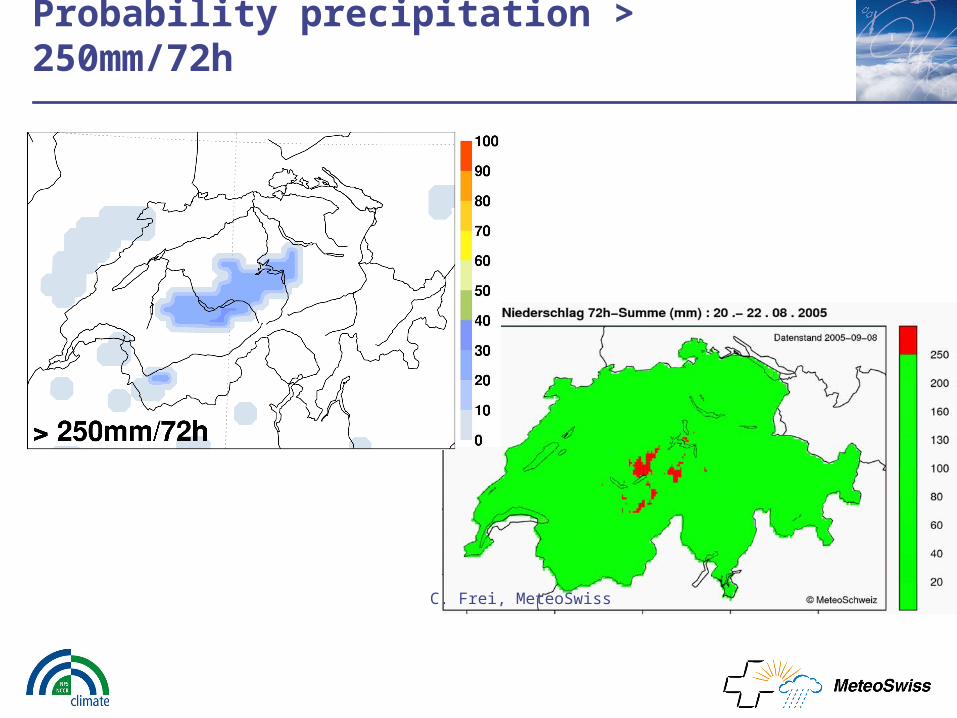
Probability precipitation > 250mm/72h

C. Frei, MeteoSwiss

Summary

COSMO-LEPS has proved to provide useful forecast uncertainty estimates for extreme events.

In the case of the flooding of August, warning has been issued on 21st August. No early warning has been given on 19th, 20st August, although aLMo, LEPS gave correct signal.

The effect of previous false alarms should not be underestimated.

Massimo Milelli, Daniele Cane

VII COSMO General MeetingZuerich, September 20-23 2005

Use of Multi-Model Super-Ensemble

Technique for complex

orography weather forecast

N

iiii FFaOS

1

N

ii OF

NOS

1

1

N

iii FF

NOS

1

1

As suggested by the name, the Multimodel SuperEnsemble method requires several model outputs, which are weighted with an adequate set of weights calculated during the so-called training period. The simple Ensemble method with bias-corrected or biased data respectively, is given by

(1) or (2)

The conventional SuperEnsemble forecast (Krishnamurti et. al., 2000) constructed with bias-corrected data is given by

(3)

Multimodel Theory

We use the following operational runs of the 0.0625° resolution version of LM (00 and 12 UTC runs)

Local Area Model Italy (UGM, ARPA-SIM, ARPA Piemonte) (nud00, nud12)Lokal Modell (Deutscher Wetterdienst) (lkd00, lkd12)aLpine Model (MeteoSwiss) (alm00, alm12)

Training: 180 days (dynamic)Forecast: from July 2004 to March 2005Stations: 102Method: mean and maximum values over warning areas

Precipitation

Me

an

Ma

xim

um

0,0

0,3

0,7

1,0

1,3

1,7

2,0

5 10 20 35

precipitation (mm)

BIA

S

-0,3

0,0

0,3

0,7

1,0

1,3

1,7

2,0

5 10 20 35 50 75

precipitation (mm)

BIA

S

0,0

0,1

0,2

0,3

0,4

0,5

0,6

5 10 20 35precipitation (mm)

ET

S

0,0

0,1

0,2

0,3

0,4

0,5

0,6

5 10 20 35 50 75precipitation (mm)

ET

S

36-60 h

We use the following operational runs of the 0.0625° resolution version of LM (00 and 12 UTC runs)

Local Area Model Italy (UGM, ARPA-SIM, ARPA Piemonte) (nud00, nud12)Lokal Modell (Deutscher Wetterdienst) (lkd00, lkd12)aLpine Model (MeteoSwiss) (alm00, alm12)

Training: 90 days (dynamic)Forecast: March 2005Stations: 53 (h<700m), 34 (700m<h<1500m), 15 (h>1500m)Method: bilinear interpolation horizontally, linear vertically (using Z)

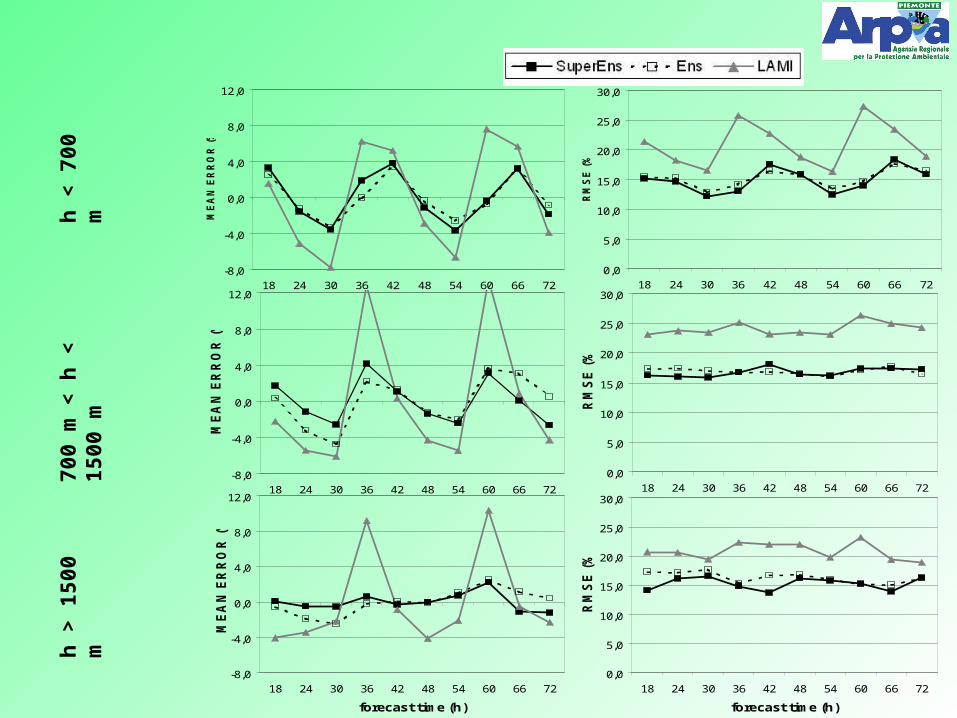
Temperature

h < 700 m

700 m < h < 1500 m

h > 1500 m

0

2

4

6

8

10

12

14

18 24 30 36 42 48 54 60 66 72

Mea

n T

emp

erat

ure

(°C

)

-1

0

1

2

3

4

5

6

7

8

18 24 30 36 42 48 54 60 66 72

Mea

n T

emp

erat

ure

(°C

)

-4

-3

-2

-1

0

1

2

3

18 24 30 36 42 48 54 60 66 72

Forecast Time (h)

Mea

n T

emp

erat

ure

(°C

)

-4,0

-2,0

0,0

2,0

4,0

18 24 30 36 42 48 54 60 66 72

ME

AN

ER

RO

R (

°C)

0,0

1,0

2,0

3,0

4,0

5,0

6,0

7,0

18 24 30 36 42 48 54 60 66 72

RM

SE

(°C

)

-4,0

-2,0

0,0

2,0

4,0

18 24 30 36 42 48 54 60 66 72

ME

AN

ER

RO

R (

°C)

0,0

1,0

2,0

3,0

4,0

5,0

6,0

7,0

18 24 30 36 42 48 54 60 66 72

RM

SE

(°C

)

-4,0

-2,0

0,0

2,0

4,0

18 24 30 36 42 48 54 60 66 72

forecast time (h)

ME

AN

ER

RO

R (

°C)

0,0

1,0

2,0

3,0

4,0

5,0

6,0

7,0

18 24 30 36 42 48 54 60 66 72

forecast time (h)

RM

SE

(°C

)

h <

700

m70

0 m

< h

< 1

500

mh

> 1

500

m

We use the following operational runs of the 0.0625° resolution version of LM (00 and 12 UTC runs)

Local Area Model Italy (UGM, ARPA-SIM, ARPA Piemonte) (nud00, nud12)Lokal Modell (Deutscher Wetterdienst) (lkd00, lkd12)aLpine Model (MeteoSwiss) (alm00, alm12)

Training: 90 days (dynamic)Forecast: March 2005Stations: 53 (h<700m), 34 (700m<h<1500m), 15 (h>1500m)Method: bilinear interpolation horizontally, linear vertically (using Z)

Relative Humidity

h <

700

m70

0 m

< h

< 1

500

mh

> 1

500

m

0,0

5,0

10,0

15,0

20,0

25,0

30,0

18 24 30 36 42 48 54 60 66 72

RM

SE

(%

)

0,0

5,0

10,0

15,0

20,0

25,0

30,0

18 24 30 36 42 48 54 60 66 72

RM

SE

(%

)

0,0

5,0

10,0

15,0

20,0

25,0

30,0

18 24 30 36 42 48 54 60 66 72

forecast time (h)

RM

SE

(%

)

-8,0

-4,0

0,0

4,0

8,0

12,0

18 24 30 36 42 48 54 60 66 72

ME

AN

ER

RO

R (

%)

-8,0

-4,0

0,0

4,0

8,0

12,0

18 24 30 36 42 48 54 60 66 72

ME

AN

ER

RO

R (

%)

-8,0

-4,0

0,0

4,0

8,0

12,0

18 24 30 36 42 48 54 60 66 72

forecast time (h)

ME

AN

ER

RO

R (

%)

Conclusions

• Multimodel Ensemble and SuperEnsemble permit a strong improvement of all the considered variables with respect to direct model output.

• In particular, SuperEnsemble is always superior to Ensemble, except for mean precipitation over warning areas and for ETS in general.

FIRST EXPERIMENTS FOR A SREPS SYSTEM

Chiara Marsigli ARPA-SIM - WG4

Basis: Operational COSMO-LEPS starting at 12 UTC of the 9th April 2005 (intense precipitation over Emilia Romagna region between 0 UTC of the 10 and 0 UTC of the 12 April 2005)

Set-up of the operational system:

model: LM version 3.9, no nudging, QI and prognostic precipitation

perturbations: b.c. and i.c. from 10 Representative Members selected out of 2 EPS; use of Tiedtke or Kain-Fritsch random

Experiment set-up:

Adding perturbations of the physical parameters of the model -> runtime perturbations

Forecast range: +72h

Member PerturbationM 1 ctrl - T (ope)

M 2 KF only (ope)

M 3 KF + crsmin=200. and c_soil=c_lnd=2

M 4 KF (no ope) + pat_len=0., c_diff=0. and tur_len=1000

M 5 T + pat_len=10000. and c_diff=2.

M 6 KF + crsmin=200., c_soil=0. and rlam_heat=50.

M 7 T (no ope) + lcape=.true.

M 8 KF + l2tls=.true.

M 9 KF + epsass=0.05

M 10 epsass=0.15 (default) + hd_corr_q=0.75

COSMO 2005

Interpretation of the new high-resolution model LMK

Heike Hoffmann heike.hoffmann@dwd.de

Volker Renner volker.renner@dwd.de

Susanne Theis susanne.theis@dwd.de

COSMO 2005

Method

We plan a two step approach

1. Using information of a single model forecast by applying the Neighbourhood Method (NM)

2. Using information resulting from LMK forecasts that are started every 3 h (LAF-Ensemble)

COSMO 2005

Assumption: LMK-forecasts within a spatiotemporal neighbourhood are assumed to constitute a sample of the forecast at the central grid point

Neighbourhood Method

COSMO 2005

Products

Smoothed fields for deterministic forecasts

• Expectation Values from spatiotemporal neighbourhood• simple averaging over quadratic grid boxes

Probabilistic Products

• Exceedance Probabilities for certain threshold values for different parameters, especially for hazardous weather warnings

COSMO 2005

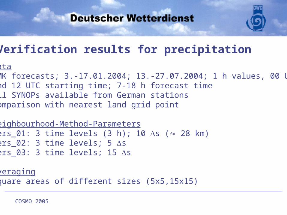
Verification results for precipitation

DataLMK forecasts; 3.-17.01.2004; 13.-27.07.2004; 1 h values, 00 UTC and 12 UTC starting time; 7-18 h forecast timeall SYNOPs available from German stationscomparison with nearest land grid point

Neighbourhood-Method-Parametersvers_01: 3 time levels (3 h); 10 s ( 28 km)vers_02: 3 time levels; 5 s vers_03: 3 time levels; 15 s

Averagingsquare areas of different sizes (5x5,15x15)

COSMO 2005

LMK, 3.-17. Jan., vv=7-18h, 00 UTC, FBI

0.0

0.2

0.4

0.6

0.8

1.0

1.2

1.4

1.6

1.8

2.0

0.1 0.2 0.5 1.0 2.0 5.0

threshold [mm/h]

LMK DMO

expectation value v2

5*5

15*15

COSMO 2005

LMK, 3.-17. Jan., vv=7-18h, 00 UTC, HSS

0

10

20

30

40

50

60

0.1 0.2 0.5 1.0 2.0 5.0threshold [mm/h]

LMK DMO

expectation value v2

5*5

15*15

COSMO 2005

LMK, 13.-27. July 2004, vv=7-18h, 00 UTC, FBI

0.0

0.5

1.0

1.5

2.0

2.5

3.0

0.1 0.2 0.5 1 2 5

threshold [mm/h]

LMK DMO

5*5

15*15

expectation value v2

COSMO 2005

LMK, 13.-27. July 2004, vv=7-18h, 00 UTC, HSS

0

5

10

15

20

25

30

35

0.1 0.2 0.5 1 2 5

threshold [mm/h]

LMK DMO

5*5

15*15

expectation value v2

COSMO 2005

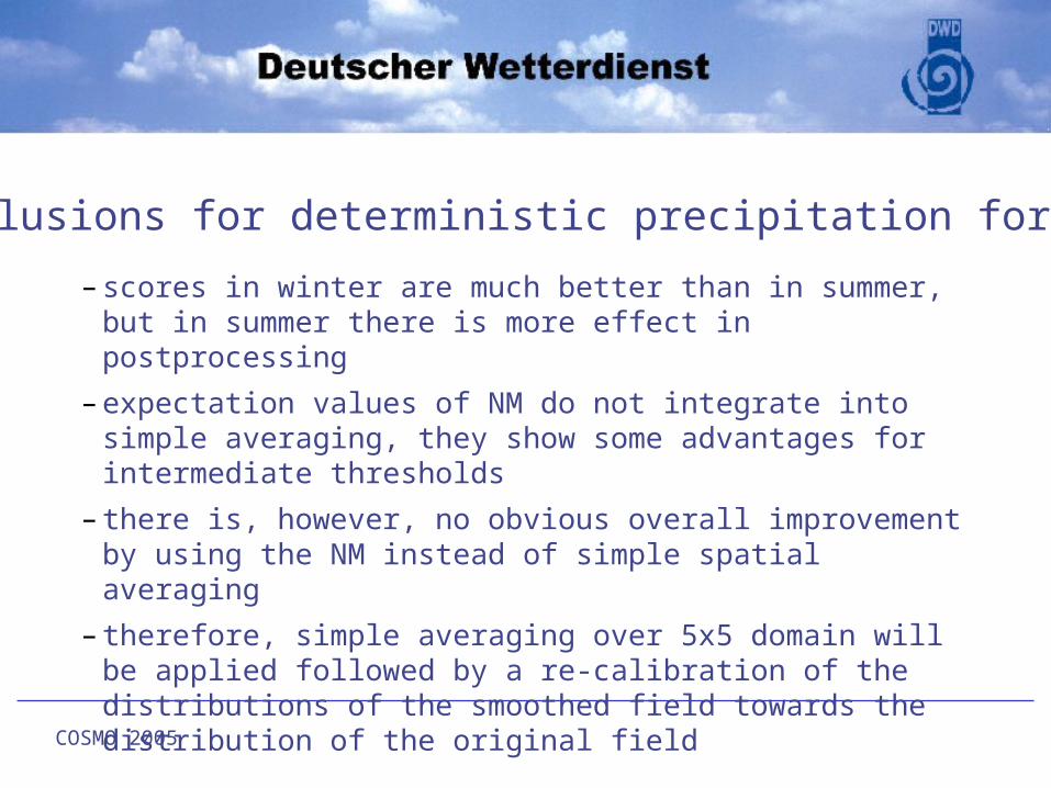
– scores in winter are much better than in summer, but in summer there is more effect in postprocessing

– expectation values of NM do not integrate into simple averaging, they show some advantages for intermediate thresholds

– there is, however, no obvious overall improvement by using the NM instead of simple spatial averaging

– therefore, simple averaging over 5x5 domain will be applied followed by a re-calibration of the distributions of the smoothed field towards the distribution of the original field

Conclusions for deterministic precipitation forecasts

COSMO 2005

LMK Total Precipitation [mm/h] 13. Jan. 2004, 00 UTC, vv=17-18h

[mm/h]

COSMO 2005

Exceedance Probability of 1mm/h, 13. Jan. 2004, 00 UTC, vv=17-18h

[%]

calculated with the NM with radius 10 grid steps, 3 time intervals (t-1, t, t+1)

COSMO 2005

LMK, BSS, 3.-17. Jan. 2004, 00 UTC

-30

-20

-10

0

10

20

30

40

50

0.1 0.2 0.5 1 2 5

threshold [mm/h]

BSS Jan v1 climate

BSS Jan v1 LMK

BSS Jan v2 LMK

BSS Jan v2 climate

COSMO General MeetingZurich, 2005

Simple Kalman filter – a “smoking gun” of shortages of models?

Andrzej MazurInstitute of Meteorology and Water Management

COSMO General MeetingZurich, 2005

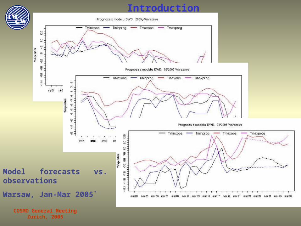
Introduction

Model forecasts vs. observations

Warsaw, Jan-Mar 2005`

COSMO General MeetingZurich, 2005

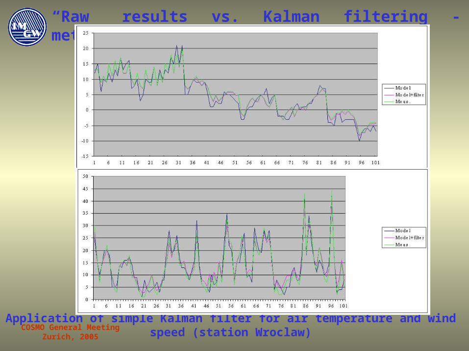
“Raw” results vs. Kalman filtering - meteograms

Application of simple Kalman filter for air temperature and wind speed (station Wroclaw)

COSMO General MeetingZurich, 2005

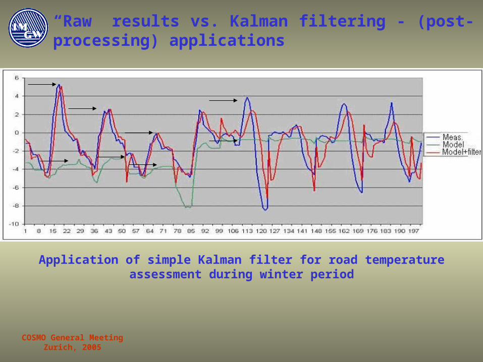
Application of simple Kalman filter for road temperature assessment during winter period

“Raw” results vs. Kalman filtering - (post-processing) applications

COSMO General MeetingZurich, 2005

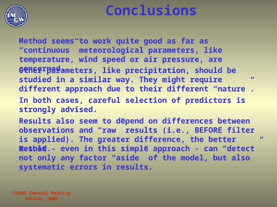
Conclusions

Method seems to work quite good as far as “continuous” meteorological parameters, like temperature, wind speed or air pressure, are concerned.

Other parameters, like precipitation, should be studied in a similar way. They might require different approach due to their different “nature”.

In both cases, careful selection of predictors is strongly advised.

Results also seem to depend on differences between observations and “raw” results (i.e., BEFORE filter is applied). The greater difference, the better result.

Method - even in this simple approach - can “detect” not only any factor “aside” of the model, but also systematic errors in results.

WP4 Intrepretation and applications

WP4 intends to propose two projects

1. Short range ensemble with own perturbations (connexions with WG1, ensemble assimilation)

2. Interpretation, grid point statistics, input to forecast matrix, input to hydrological models