Embed Size (px)
Citation preview

OPERATIONS RESEARCHVol. 65, No. 2, March–April 2017, pp. 446–468
http://pubsonline.informs.org/journal/opre/ ISSN 0030-364X (print), ISSN 1526-5463 (online)
The Impact of Linear Optimization on Promotion PlanningMaxime C. Cohen,a Ngai-Hang Zachary Leung,b Kiran Panchamgam,c Georgia Perakis,d Anthony Smithc
a Stern School of Business, New York University, New York, New York 10012; bCollege of Business, City University of Hong Kong, Kowloon,Hong Kong; cOracle Retail Global Business Unit (RGBU), Burlington, Massachusetts 01803; d Sloan School of Management, MassachusettsInstitute of Technology, Cambridge, Massachusetts 02139Contact: [email protected] (MCC); [email protected] (N-HZL); [email protected] (KP);[email protected] (GP); [email protected] (AS)
Received: January 20, 2014Revised: August 7, 2015; June 27, 2015Accepted: September 23, 2016Published Online in Articles in Advance:January 19, 2017
Subject Classifications: programming: integer,linear/applications, nonlinear/applicationsArea of Review: Optimization
https://doi.org/10.1287/opre.2016.1573
Copyright: © 2017 INFORMS
Abstract. Sales promotions are important in the fast-moving consumer goods (FMCG)industry due to the significant spending on promotions and the fact that a large pro-portion of FMCG products are sold on promotion. This paper considers the problem ofplanning sales promotions for an FMCG product in a grocery retail setting. The cate-gory manager has to solve the promotion optimization problem (POP) for each product,i.e., how to select a posted price for each period in a finite horizon so as to maximizethe retailer’s profit. Through our collaboration with Oracle Retail, we developed an opti-mization formulation for the POP that can be used by category managers in a groceryenvironment. Our formulation incorporates business rules that are relevant, in practice.We propose general classes of demand functions (including multiplicative and additive),which incorporate the post-promotion dip effect, and can be estimated from sales data. Ingeneral, the POP formulation has a nonlinear objective and is NP-hard. We then proposea linear integer programming (IP) approximation of the POP. We show that the IP has anintegral feasible region, and hence can be solved efficiently as a linear program (LP). Wedevelop performance guarantees for the profit of the LP solution relative to the optimalprofit. Using sales data from a grocery retailer, we first show that our demand modelscan be estimated with high accuracy, and then demonstrate that using the LP promotionschedule could potentially increase the profit by 3%, with a potential profit increase of 5%if some business constraints were to be relaxed.
Funding: This work was also partly supported by the National Science Foundation [Grant CMMI-1162034].
Supplemental Material: The online appendix is available at https://doi.org/10.1287/opre.2016.1573.
Keywords: promotion optimization • dynamic pricing • integer programming • retail operations
1. IntroductionFast-moving consumer goods (FMCG) or consumerpackaged goods (CPG) are products, which are con-sumed quickly. Examples of FCMG include processedfoods and drinks (e.g., canned food, soft drinks,salty snacks, candy, and chocolate) as well as house-hold products (e.g., toiletries, laundry detergent). TheFMCG industry includes some of the most widely rec-ognized companies in the world, such as Coca-Cola,Pepsico, Kraft, Nestle, Proctor & Gamble, Johnson &Johnson, and Unilever. Typically, consumers do notpurchase FMCG products directly from manufactur-ers, but rather from retailers (supermarkets and gro-cery stores).It is common for manufacturers and retailers in the
FMCG industry to use promotions to entice consumersto purchase their products. The reasons why promo-tions are used include: increasing sales and traffic,introducing new items, bolstering customer loyalty,competitive retaliation, and price discrimination. Theamount of money spent on promotions is significant—it is estimated that FMCG manufacturers spend about
$1 trillion annually on promotions (Nielsen 2014).In addition, promotions play an important role inthe FMCG industry as a significant proportion ofsales are made on promotion. For example, Nielsen(Nielsen 2014) found that 12%–25% of supermarketsales in five European countries (Great Britain, Spain,Italy, Germany, and France) were made on promotion(Gedenk et al. 2006). Not all retailers use promotions—some retailers (e.g., Walmart) employ an everyday lowprice policy. In this paper, we focus on retailers that useprice promotions.
A promotion tactic that is commonly used by retail-ers is temporary price reductions. We illustrate the effec-tiveness of temporary price reductions in boostingsales using real data. In Figure 1, we plot the weekly(normalized) prices and sales for a particular brandof ground coffee in a supermarket over 35 weeks. Weobserve that this brand was promoted during 8 out of35 weeks (i.e., 23% of the time); and that promotionalsales accounted for 41% of the total sales volume. Inthis paper, we focus on temporary price reductions bygrocery retailers that we simply refer to as promotions.
446

Cohen et al.: The Impact of Linear Optimization on Promotion PlanningOperations Research, 2017, vol. 65, no. 2, pp. 446–468, ©2017 INFORMS 447
Figure 1. Prices and sales for a particular brand of coffee at asupermarket over a span of 35 weeks
0.8
0.9
1.0
Pric
e
85 90 95 100 105 110 115 120500
1,000
1,500
2,000
Week
Vol
ume
of s
ales
Promotions can have a significant impact on aretailer’s profitability. Using a demand model esti-mated from sales data (see Section 7.3 for details),we estimate that the promotions set by the retailerachieved a profit gain of 3% compared to using onlythe regular price (i.e., no promotions). A paper pub-lished by the Community Development Financial Insti-tutions Fund reports that the average profit margin forthe supermarket industry was 1.9% in 2010. Accord-ing to an analysis performedwith Yahoo! Finance data,the average net profit margin for publicly traded U.S.-based grocery stores for 2012 is close to 2010’s 1.9%average. As a result, this suggests that promotionscan have a significant impact on the retailer’s profits.Furthermore, this motivates us to build a model thatanswers the following question: How much moneydoes the retailer leave on the table by using theimplemented prices relative to “optimal” promotionalprices?
Given the importance of promotions in the groceryindustry, it is not surprising that supermarkets paygreat attention to design promotion schedules. Thepromotion planning process is complex and challeng-ing for multiple reasons. First, demand is affected bya post-promotion dip effect, i.e., for certain categories ofproducts, promotions lead to reduced future demand.Second, promotions are constrained by a set of busi-ness rules specified by the supermarket and/or prod-uct manufacturers. Example of business rules includeprices chosen from a discrete set, limited number ofpromotions, and separating successive promotions (formore details, see Section 3.2). Finally, the problem isdifficult even for a single retail store because of its largescale. For instance, a typical supermarket in the UnitedStates carries about 40,000 SKUs, with approximately2,000 SKUs on promotion at any point in time, whichleads to a very large number of decisions variables.
Despite the complexity of the promotion planningprocess, it is still to this day, performed manually inmost supermarkets. This motivates us to design andstudy promotion optimization models that can make
promotion planning more efficient (reducing man-hours), and at the same time, more profitable (increas-ing profits and revenues) for retailers.
To accomplish this, we introduce a promotion opti-mization problem (POP) formulation and propose howto solve it efficiently. We introduce and study classes ofdemand functions that incorporate the features we dis-cussed above as well as constraints that model impor-tant business rules. The output will provide optimizedprices together with performance guarantees. In addi-tion, because our formulation can be solved quickly, amanager can test various what-if scenarios to study therobustness of the solution.
Our proposed POP formulation is a nonlinear inte-ger programming (IP). For general demand functions,the formulation is NP-hard (see Cohen et al. 2016). Animportant business rule for retailers, in practice, is thatthe price of the product must be selected from a priceladder, i.e., a discrete set of permissible prices. In addi-tion, due to the post-promotion dip effect, for generaldemand functions, the objective is neither concave norconvex. We therefore propose a linear IP approxima-tion and show that the problem can be solved effi-ciently as an LP. This new formulation approximatesthe POP problem for a general demand. In addition,we derive analytical lower and upper bounds relativeto the optimal objective that rely on the structure ofthe POP objective with respect to promotions. In par-ticular, we show that when past prices have a multi-plicative effect on current demand, for a certain subsetof promotions, the profits are submodular in pro-motions, whereas when past prices have an additiveeffect, the profits are supermodular in promotions. Inthis context, submodular (supermodular) means thatthe marginal effect on an additional promotion has asmaller (larger) impact when we already have manypromotions in the selling season. These results allowus to derive guarantees on the performance of the LPapproximation relative to the optimal POP objective.We also extend our analysis to the case of a combineddemand model where both structures of past pricesare simultaneously considered. Finally, we show usingactual data that the models run fast, in practice, andcan yield increased profits for the retailer.
The impact of our models can be also significantfor supermarkets, in practice. One of the goals of thisresearch has been to develop data-driven optimizationmodels that can guide the promotion planning pro-cess for grocery retailers, including the clients of OracleRetail. They span the range of midmarket (annual rev-enue below $1 billion) as well as Tier 1 (annual revenueexceeding $5 billion and/or 250+ stores) retailers allover the world. One key challenge for implementingour models into software is the large-scale nature ofthis industry. For example, a typical Tier 1 retailer hasapproximately 1,000 stores, with 200 categories each

Cohen et al.: The Impact of Linear Optimization on Promotion Planning448 Operations Research, 2017, vol. 65, no. 2, pp. 446–468, ©2017 INFORMS
containing 50–600 items. An important criterion for ourmodels to be adopted by grocery retailers, is that thesoftware tool needs to run in a few seconds up to aminute. This motivated us to reformulate our model asan LP.Preliminary tests using supermarket sales data sug-
gest that our model can increase profits by 3% just byoptimizing the promotion schedule, and up to 5% byslightly increasing the number of promotions allowed.If we assume that implementing the promotions rec-ommended by our models does not require additionalfixed costs (this seems to be reasonable as we only varyprices), then a 3% increase in profits for a retailer withannual profits of $100 million translates into a $3 mil-lion increase. As we previously discussed, profit mar-gins in this industry are thin, and therefore 3% profitimprovement is significant.
ContributionsThis research was conducted in collaboration with ourcoauthors and industry practitioners from the OracleRetail Science group, which is a business unit of OracleCorporation. One of the end outcomes of this work isthe development of sales promotion analytics that willbe integrated into enterprise resource planning soft-ware for supermarket retailers.
• We propose a POP formulation motivated by real-world retail environments. We introduce a nonlinear IPformulation for the single-item POP. Unfortunately,this model is not computationally tractable, in gen-eral. An important requirement from our industrycollaborators is that an executive of a medium-sizedsupermarket (100 stores, ∼200 categories, ∼100 itemsper category) can run a software tool embedding themodel and algorithms in this paper and obtain a high-quality solution in a few seconds. This motivates us topropose an LP approximation.
• We propose an LP reformulation that allows us tosolve the problem efficiently. We first introduce a linearIP approximation of the POP. We then show that theconstraint matrix is totally unimodular, and thereforethe IP can be solved efficiently as an LP.
• We introduce general classes of demand functions thatmodel the post-promotion dip effect. An important featureof the application domain is the post-promotion dipin demand observed, in practice. We propose generalclasses of demand functions inwhich past prices have amultiplicative or an additive effect on current demand.These classes are generalizations of models commonlyused in the literature, provide modeling flexibility andcan be estimated from data.
• We develop tight bounds on performance guarantees formultiplicative and additive demand functions. We deriveupper and lower guarantees on the quality of the LPapproximation relative to the optimal (but computa-tionally intractable) POP solution, and characterize the
bounds as a function of the problem parameters. Weshow that for multiplicative demand, promotions havea submodular effect (for some relevant subsets of pro-motions). This leads to the LP approximation being anupper bound of the POP objective.
• We validate our results using actual data and demon-strate the added value of our model. Our industry part-ners provided us with a collection of sales data fromseveral product categories. We apply our analysis to afew selected categories (ground coffee, tea, chocolate,and yogurt). We first estimate the demand parametersand then quantify the value of our LP approximationrelative to the optimal POP solution. After extensivenumerical testing with the clients’ data, we show thatthe approximation error is, in practice, even smallerthan the analytical bounds we developed. Our modelprovides supermarket managers recommendations forpromotion planning with running times in the orderof seconds. As the model runs fast and can be imple-mented on a platform like Excel, it allows managersto test and compare various strategies easily. By com-paring the predicted profit under the actual prices tothe predicted profit under our LP optimized prices, wequantify the added value of our model.
• We demonstrate that our results are robust with respectto demand uncertainty. We propose a way to addressthe case where the estimated demand parameters areuncertain. We then validate the robustness of our solu-tion using actual data. In particular, extensive testingsuggests that the profit gain dominates the forecastingerror.
2. Literature ReviewOur work is related to four streams of literature: opti-mization, marketing, dynamic pricing, and retail oper-ations.We formulate the POP for a single item as a non-linear mixed-integer program (NMIP). To give usersflexibility in the choice of demand functions, our POPformulation imposes very mild assumptions on thedemand. Due to the general classes of demand func-tions, we consider the objective is typically nonconcave.In general, NMIPs are difficult from a computationalcomplexity standpoint. Under certain special struc-tural conditions (e.g., see Hemmecke et al. 2010 andreferences therein), there exist polynomial-time algo-rithms for solving NMIPs. However, many NMIPs donot satisfy these special conditions and are solvedusing techniques such as branch and bound, outer-approximation, generalized benders, and extendedcutting plane methods (Grossmann 2002).
In a special instance of the POP when demand is alinear function of current and past prices andwhen dis-crete prices are relaxed to be continuous, one can for-mulate the POP as a cardinality-constrained quadraticoptimization (CCQO) problem. It has been shown inBienstock (1996) that a quadratic optimization problem

Cohen et al.: The Impact of Linear Optimization on Promotion PlanningOperations Research, 2017, vol. 65, no. 2, pp. 446–468, ©2017 INFORMS 449
with a similar feasible region as the CCQO is NP-hard.Thus, tailored heuristics have been developed (see, e.g.,Bertsimas and Shioda 2009, Bienstock 1996).Our solution approach is based on linearizing the
objective function by exploiting the discrete nature ofthe problem, and then solving the POP as an LP. Wenote that due to the general nature of the demand func-tions, we consider it is not possible to use linearizationapproaches such as in Sherali and Adams (1998) orFletcher and Leyffer (1994). We refer the reader to thebooks by Nemhauser andWolsey (1988) and BertsimasandWeismantel (2005) for IP reformulation techniquesto potentially address the nonconvexities. However, weobserve that most of them are not directly applicableto our problem since the objective of interest is a timedependent neither convex nor concave function.
Our work is related to linearization techniques fornonlinear IP problems. One common procedure inthis field is to add additional constraints, and possi-bly introduce new variables, to produce tight (usuallylinear) relaxations. It is, of course, necessary to provethat the new problem is equivalent to the initial one.We briefly describe two important works in this area.In Adams et al. (2004), the authors present a strategyfor finding a tighter linear relaxation of a mixed 0-1quadratic program. In Chaovalitwongse et al. (2004),the authors propose a new linearization method forquadratic 0-1 programming problems with linear andquadratic constraints, which requires only O(kn) addi-tional continuous variables where k denotes the num-ber of quadratic constraints.In this paper, we formulate the POP as a nonlin-
ear binary IP problem. Due to the general nature ofthe demand functions, to the best of our knowledge,none of the existing approaches in the literature applydirectly to our formulation. Instead of solving the non-linear problem exactly, we consider an approximationbased on linearizing the nonlinear objective function.The linearization uses the sum of the marginal contri-butions of a single promotion, and can be viewed asa first-order Taylor approximation of the total profitsaround the regular prices. By showing that the con-straint matrix of the integer program is totally unimod-ular, solving the linear relaxation yields the optimalIP solution. By exploiting the structure of the demandfunctions, we derive provable performance guaranteesfor our solution method.
As we show later in this paper, the POP for the twoclasses of demand functions we introduce is related tosubmodular and supermodular maximization. Maxi-mizing an unconstrained supermodular function wasshown to be a strongly polynomial-time problem (see,e.g., Schrijver 2000). In our case, we have severalconstraints on the promotions, and as a result, it isnot guaranteed that one can solve the problem effi-ciently to optimality. In addition, most of the pro-posed methods to maximize supermodular functions
are not easy to implement and are often not very prac-tical in terms of running time. Indeed, our industrycollaborators request solving the POP in at most fewseconds and using an available platform like Excel.Unlike supermodular objectives, maximizing a sub-modular function is generally NP-hard (see, for exam-ple, McCormick 2005). Several common problems,such as max cut and the maximum coverage problem,can be cast as special cases of this general submodu-lar maximization problem under suitable constraints.Typically, the approximation algorithms are based oneither greedy methods or local search algorithms.The problem of maximizing an arbitrary nonmono-tone submodular function subject to no constraintsadmits a 1/2 approximation algorithm (see, for exam-ple, Buchbinder et al. 2012, Feige et al. 2011). In addi-tion, the problem of maximizing a monotone submod-ular function subject to a cardinality constraint admitsa 1 − 1/e approximation algorithm (e.g., Nemhauseret al. 1978). In our case, we propose an LP approxi-mation that does not request any monotonicity or anystructure on the objective. This LP approximation alsoprovides a guarantee relative to the optimal profit fortwo classes of demand. Nevertheless, these bounds areparametric and not uniform. To compare them to theexisting methods, we compute in Section 7, the valuesof these bounds on different demand functions esti-mated with actual data.
Sales promotions are well studied in marketing (seeBlattberg and Neslin 1990, and the references therein).The marketing community has observed that for manyFMCG products, temporary price reductions lead toa future demand reduction, a phenomenon that isreferred to as the post-promotion dip effect. Marketingresearchers typically focus on developing and estimat-ing demand models, e.g., linear regression or choicemodels, to derive managerial insights on promotions(Cooper et al. 1999, Foekens et al. 1998). For example,Foekens et al. (1998) study parametric econometricsmodels based on scanner data to examine the dynamiceffects of sales promotions. One of the methods used inthe marketing literature to capture the post-promotiondip effect is to use a demand function that dependsnot only on the current price, but also on the prices atthe most recent periods (Mela et al. 1998, Heerde et al.2000, Macé and Neslin 2004, Ailawadi et al. 2007).
Our work is also related to the field of dynamicpricing (see, e.g., Talluri and van Ryzin 2005 and thereferences therein). More specifically, in the opera-tions management literature, researchers study salespromotions from the angle of how to optimize thedynamic pricing of a product given that consumerbehavior leads to post-promotion dips in demand. Oneapproach is to build a game-theoretic model of con-sumers. In Assunção and Meyer (1993), the authorsconsider the problem faced by a rational consumer

Cohen et al.: The Impact of Linear Optimization on Promotion Planning450 Operations Research, 2017, vol. 65, no. 2, pp. 446–468, ©2017 INFORMS
regarding optimal purchasing and consumption of astorable good. In their model, the price in the nextperiod is assumed to be random (drawn from a sta-tionary distribution of prices conditional on the lastobserved price). In addition, the authors assume thatthe seller’s pricing policy is exogenous and random.In Su (2010), the author develops a model with mul-tiple consumer types who may differ in their hold-ing costs, consumption rates, and fixed shopping costs.The author could solve the dynamic pricing modelfor the rational expectation equilibrium, and drawsseveral managerial insights. An alternative approachused in the dynamic pricing literature is to model con-sumers using a reference price model (Kopalle et al.1996, Fibich et al. 2003, Popescu and Wu 2007, Chenet al. 2016). The reference price model posits that con-sumers form an internal reference price for the productbased on past price observations. When the consumerobserves the current price, she compares it to the ref-erence price as a benchmark. Prices above the refer-ence price are perceived to be “high,” which leadsto lower demand, whereas prices below the referenceprice are perceived to be “low,” leading to an increasein demand. The papers by Kopalle et al. (1996), Fibichet al. (2003), Popescu and Wu (2007) study an infinite-horizon dynamic pricing problem with a referenceprice model. In Chen et al. (2016), the authors ana-lyze a periodic review stochastic inventory model inwhich pricing and inventory decisions aremade simul-taneously. Our paper differs from the models in thedynamic pricing literature in that our dynamic pricingproblem includes business rules that are relevant, inpractice.In Ahn et al. (2007), the authors propose a demand
model in which a proportion of customers will wait kperiods after andwill purchase once the posted price ofthe product falls below their willingness to pay. Underthis assumption, their demand model depicts the post-promotion dip effect.In this paper, we propose two general classes of mul-
tiplicative and additive demand models. The multipli-cative model is a generalization of the linear regres-sion model with lagged variables used by Heerdeet al. (2000), Macé and Neslin (2004). In addition, thedemand model we propose can closely approximatethe reference price model used in Kopalle et al. (1996),Fibich et al. (2003), Popescu and Wu (2007); as wellas the demand model in Ahn et al. (2007). Finally,our work is related to the field of retail operations,and more specifically, pricing problems under busi-ness rules. One of the constraints considered in ourpaper imposes the prices to lie in a discrete set. Zhaoand Zheng (2000) consider a dynamic pricing prob-lem for a fixed inventory perishable product sold overa finite- (continuous) time horizon. For the case of adiscrete price set, the authors solve the continuous
time dynamic program by applying a discretizationapproach and a backward recursion. The computa-tional complexity of their approach grows linearlywiththe number of discrete-time intervals. Our approach isdifferent in nature and is based on an LP approxima-tion that yields a complexity polynomial in the numberof time periods. Subramanian and Sherali (2010) studya pricing problem for grocery retailers, where pricesare subject to interitem constraints. They propose a lin-earization technique to solve the problem. Caro andGallien (2012) study amarkdown pricing problem for afashion retailer, for which the prices are constrained tobe nonincreasing, and some set of items are restrictedto have the same prices over time.
The remainder of the paper is structured as fol-lows. In Section 3, we describe the model, the assump-tions, the business rules, and we formulate the POP.In Section 4, we present an approximate formulationbased on linearizing the objective, which gives riseto a linear IP. We then show that the IP can, in fact,be solved as an LP. In Section 5, we consider mul-tiplicative and additive demand models and derivetight bounds on the LP approximation relative to theoptimal solution. In Section 6, we consider an exten-sion of our approach for uncertain demand. Section 7presents computational results using real data. Finally,we present our conclusions. Several of the proofs ofthe different propositions and theorems are relegatedto the appendix.
3. Model, Assumptions, andProblem Formulation
In this section, we present a mathematical model ofthe POP for an FMCG product. One of our primarygoals is to incorporate problem features that are rel-evant, in practice. The model was developed througha collaboration with our coauthors working at OracleRetail, and thus we have benefited from the expertiseof Oracle executives as well as retailers.
The manager of an FMCG category in a groceryretailer faces the POP: for a given product, how to selecta posted price for each period in a finite sales horizonso as to maximize the retailer’s profit. In the following,we describe the assumptions underlying our formula-tion (see Section 3.1) as well as the business rules (seeSection 3.2). Finally, we present a mathematical formu-lation of the POP in Section 3.3.
3.1. AssumptionsIn this paper, we focus on a single-item model of thePOP.
Assumption 1 (Cost of Inventory). At each period t, theretailer orders inventory from the supplier at a unit cost ct .

Cohen et al.: The Impact of Linear Optimization on Promotion PlanningOperations Research, 2017, vol. 65, no. 2, pp. 446–468, ©2017 INFORMS 451
The above assumption holds under the conventionalwholesale price contract, which is frequently used,in practice, and in the academic literature (see, e.g.,Cachon and Lariviere 2005, Porteus 1990).
Assumption 2 (Demand is a Deterministic Function ofPrices). The demand in period t is a deterministic functionof the prices chosen by the retailer (p1 , p2 , . . . , pT).
Here, T denotes the length of the horizon. Thisassumption is reasonable for FMCG products becausethe prices can be used to accurately forecast demand.This assumption is also supported by our experiments,which show that a regressionmodel using past prices isable to predict future demand with a low forecast error(see estimation results in Section 7 and Figure 4). Sincethe estimated deterministic demand functions seem toaccurately model actual demand, for this application,we can use them as input to the optimization modelwithout taking into account demand uncertainty. Wealso propose an extension of our approach to relaxthe deterministic demand assumption, and address thecase where demand is uncertain (see Section 6).
The typical process, in practice, is to estimate a de-mand model from data and then to compute the opti-mal prices based on the estimated demand model. InSection 7, we start with actual sales data from a super-market, estimate a demand model, and compute theoptimal prices using our model. The demand modelswe consider are commonly used by practitioners andthe academic literature (see Heerde et al. 2000, Macéand Neslin 2004, Fibich et al. 2003).
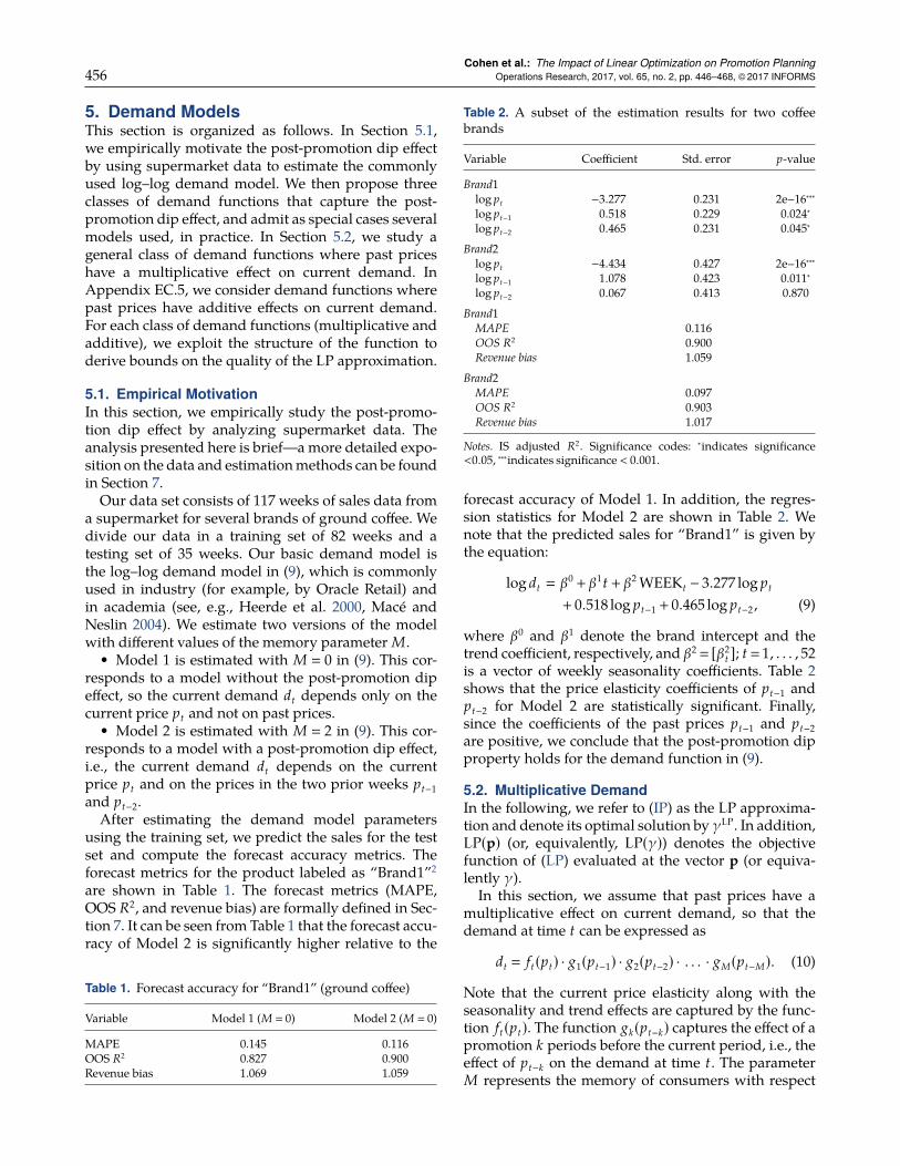
Post-Promotion Dip in Demand. Aswementioned, thedemand of an FMCG product often has the post-promotion dip property. In particular, promoting theproduct in period u < t, may reduce the demand inperiod t (relative to the demand value if the productwas not promoted at time u). This is illustrated in Fig-ure 2. We model the post-promotion dip property byassuming that the demand is a function of the currentprice and the prices in the M most recent periods:
dt(pt)� ht(pt , pt−1 , . . . , pt−M). (1)
Figure 2. Illustration of the post-promotion dip effect
1 2 3 4 5 6 7 80
100
200
300
Week
Dem
and
No promotionWith promotion
Notes. A promotion in week 3 boosts the demand in week 3, butdecreases the demand in the following weeks. Demand then gradu-ally recovers up to the no-promotion level.
It has been recognized in the marketing literaturethat in some retail settings, following a promotion,there is a decline in sales relative to what sales wouldhave been in the absence of a promotion. This isreferred to as a post-promotion dip in sales (see, e.g., Macéand Neslin 2004).
There are multiple possible explanations regard-ing the post-promotion dip effect. One explanation isthat consumers respond to promotions by purchasinglarger quantities, which they stockpile for future con-sumption. Another explanation is related to the refer-ence price effect. Very often, consumers form a referenceprice for the product, which is a weighted average ofthe recent observed prices. The current demand is thenaffected not only by the current price, but also by thereference price, through the psychological effect of feel-ing a gain or a loss. If the current price is higher thanthe reference price, consumers perceive the currentprice as a loss, which decreases demand; conversely,if the current price is lower than the reference price,consumers perceive the current price as a gain, whichincreases demand. The reference price model has beenused in dynamic pricing problems, see, e.g., Kopalleet al. (1996), Fibich et al. (2003), Popescu andWu (2007),Chen et al. (2016).
Alternatively, instead of looking at individual priceeffects on demand, one may look at the difference be-tween the effect of the current price pt relative to someweighted average of past prices (e.g., pt−1 and pt−2when M � 2). Equivalently, the consumers use somesort of weighted average as a reference point. Then, thetwo following effects may be observed.
(a) Comparison effect: Consider the case where thecurrent price pt is higher relative to the past prices pt−1and pt−2. Then, compared to the possibility that theconsumers could have purchased the product at lowerprices in the past, buying the product at this time (withthe higher price pt) feels like a loss to consumers. Thegreater the difference between pt and pt−1 (or pt−2) is,the greater the sensation of loss the consumers feel forbuying now. Such a comparison induces the consumersto become less willing to buy at pt , hence decreasingthe demand.
(b) Attachment effect: Consider now the case wherethe current price pt is smaller relative to the past pricespt−1 and pt−2. As the consumers were expecting to paya higher price, purchasing the product at the lowerprice pt feels like a gain. In addition, the greater thedifference between pt−1 (or pt−2) and pt is, the greaterthe sensation of gain the consumers feel. Therefore, theconsumers becomemore attached to the idea of buyingat this period due to this gain feeling. This attachmenteffect increases the consumers’ willingness as well asthe demand.Assumption 3 (Sufficient Inventory). The retailer has suf-ficient inventory to meet demand in each period, i.e., sales isequal to demand.

Cohen et al.: The Impact of Linear Optimization on Promotion Planning452 Operations Research, 2017, vol. 65, no. 2, pp. 446–468, ©2017 INFORMS
Remark 1. The assumption that the retailer carriesenough inventory to meet demand does not apply toall products and all retail settings. For example, it iscommon practice in the fashion industry (e.g., Talbotsor Zara) to intentionally produce limited amounts ofinventory. By doing so, a retailer sends a signal to con-sumers that they should buy the product now at theregular price. If the consumers decide to wait until theclearance season, there is a risk that the product wouldbe sold out. Consumers also expect products to stockout as the seasons change (e.g., spring to summer).
Unlike fashion items, which go out of season, FMCGproducts such as ground coffee or soft drinks are typi-cally available all year round. These products typicallyhave shelf lives greater than six months, and customershave been conditioned to expect that these productswould always be in stock at retail stores. Since theseproducts are easy to store and have a high degree ofavailability, FMCG retailers typically do not use therisk of stock out to incentivize consumers to buy now.
In addition, as we will show in our computationalexperiments, the demand forecast accuracy is high andthe out-of-sample (OOS) metrics are very good (theOOS R2 and mean absolute percentage error (MAPE)).In the data we have, we actually observed that theinventory was not issue and saw very few events ofstock-outs over a two-year period. This can be justifiedby the fact that supermarkets have a long experiencewith inventory decisions and accumulated large datasets allowing them to develop sophisticated forecastingdemand tools to support capacity and ordering deci-sions. Many such models were developed in the lasttwo decades (e.g., Cooper et al. 1999, Van Donselaaret al. 2006). Finally, it seems reasonable that con-sumers buying behavior is easier to predict for gro-cery products such as ground coffee, relative to fashionitems, which are unique and have short product cycles.Indeed, fashion involves an impulsive and occasionalpurchasing behavior (and hence can be harder to pre-dict), whereas grocery items are more routinely-basedpurchases. Finally, grocery retailers are aware of thenegative effects of stocking out of promoted products(see, e.g., Corsten and Gruen 2004, Campo et al. 2000).For all of the above reasons, the statement in Assump-tion 3 that the retailer carries sufficient inventory tomeet demand in each period is reasonable in the con-text of FMCG products.
3.2. Business RulesBusiness Rule 1 (Discrete Price Ladder). In each pe-riod t, the price pt must be chosen from a price ladder,i.e., a set of admissible prices {q0 > q1 > · · ·> qK}, whereq0 is the regular price and q1 , . . . , qK are possible pro-motional prices.
We can model the business rule mathematically bywriting the price at time t as follows:
pt �
K∑k�0
qkγkt , (2)
where γkt is a binary variable that is equal to 1 if the
price qk is selected at time t, and 0 otherwise. There-fore, instead of using the prices pt as the set of decisionvariables, we use the set of binary variables {γk
t : t �1, . . . ,T, k � 0, . . . ,K}, which is a total of (K + 1)T vari-ables. To ensure that a single price is selected for eachtime period t, we impose the additional constraints:
K∑k�0
γkt � 1 ∀ t .
Business Rule 1 is in contrast to the assumptionmade by other papers such as Popescu and Wu (2007),Kopalle et al. (1996), where the retailer can choose con-tinuous prices. Note that, in practice, the retailer canonly charge discrete prices. In the supermarket appli-cations that we were involved in, this was an importantbusiness rule.1 More precisely, the price for each itemat each time period is selected from a discrete set ofprices that consists of a regular price and levels of dis-counts. In supermarket applications, for example, thesediscounted prices have to end by 9 cents or sometimesby 5 cents.
Remark 2 (Extension to Time-Dependent Price Ladder).For clarity, in this paper, we make the simplifyingassumption that the price ladder is time independent,i.e., one can charge pt � qk for all t and k.
One can extend the analysis and results of this paperto the case where the price ladder is time dependent,i.e., the price ladder for period t is given by �t
� {q0t >
q1t > · · · > qKt
t }. Note that the number of permissibleprices and the minimal price qKt
t can be time depen-dent. In this case, Equation (2) becomes: pt �
∑Kk�0 qk
t γkt .
Business Rule 2 (Limited Number of Promotions). Theretailer may have to limit the number of promotions fora given product. This requirement is motivated fromthe fact that retailerswish to preserve the image of theirstore and not to train customers to be deal seekers. Forexample, it may be required to promote a particularproduct at most L � 3 times during the quarter. Thisconstraint can be expressed mathematically as follows:
T∑t�1
K∑k�1
γkt 6 L. (3)
Business Rule 3 (Separating Periods between Consecu-tive Promotions). A common additional requirement isto space out two successive promotions by a minimalnumber of separating periods, denoted by S. Indeed, if

Cohen et al.: The Impact of Linear Optimization on Promotion PlanningOperations Research, 2017, vol. 65, no. 2, pp. 446–468, ©2017 INFORMS 453
successive promotions are too close to one another, thismay hurt the store image and incentivize consumers tobehave more as deal seekers. In addition, this type ofbusiness requirement is often dictated directly by themanufacturer that wants to restrict the frequency ofpromotions to preserve the image of the brand. Math-ematically, we have
t+S∑τ�t
K∑k�1
γkτ 6 1 ∀ t . (4)
It is important to understand why, in practice, Busi-ness Rules 2 and 3 are commonly adopted by FMCGretailers to limit the frequency of price promotions.From an optimization point of view, these businessrules appear to be unnecessarily restrictive. Mathe-matically, the larger the promotion limit L and thesmaller the separating periods S, the larger the feasibleregion of the optimization problem, and therefore thegreater the optimal profit. Although relaxing or remov-ing Business Rules 2 and 3 will increase short-termprofitability, retailers still follow these business rulesas they recognize that running promotions too fre-quently, can hurt their long-term profit. Frequent pro-motions can negatively affect a retailer’s brand imageby conditioning consumers to perceive regular pricesas bad deals. Finally, we note that, in some cases, Busi-ness Rules 2 and 3 may be soft constraints. In thiscase, one can perform a sensitivity analysis by solv-ing the POP for different values of L and S (see suchan example in Section 7.3). If a slight change in theparameters could lead to a significant increase in profit,upper management could be convinced to relax theconstraints on L and S by renegotiatingwith the appro-priate manufacturer.
3.3. Problem FormulationWe next present our formulation of the single-itemPOProblem:
maxγk
t
T∑t�1(pt − ct)dt(pt)
s.t. pt �
K∑k�0
qkγkt
T∑t�1
K∑k�1
γkt 6 L
t+S∑τ�t
K∑k�1
γkτ 6 1 ∀ t
K∑k�0
γkt � 1 ∀ t
γkt ∈ {0, 1} ∀ t , k ,
(POP)
where:• T—Number of weeks in the horizon (e.g., one
quarter composed of 13 weeks).
• L—Limitation on the number of promotions.• S—Number of separating periods (separation
time between two successive promotions).• Q� {q0 > q1 > · · ·> qk > · · ·> qK}—Price ladder, i.e.,
the discrete set of admissible prices.• q0—Regular (nonpromoted) price, which is the
maximum price in the price ladder.• qK—Minimum price in the price ladder.• ct—Unit cost of the item at time t.Note that the only decisions are which price to
choose from the price ladder at each time (i.e.,the binary variables γk
t ). We denote by POP(p) (orequivalently, POP(γ)) the objective function of (POP)evaluated at the vector p (or equivalently, γ). This for-mulation can be applied to a general time-dependentdemand function dt(pt) that explicitly depends on thecurrent price pt , and on the M past prices as well as ondemand seasonality and trend. Specific examples arepresented in Section 5.
Remark 3 (End-of-Horizon Effects). The POP formula-tion above may be affected by the end-of-horizon effect(see, e.g., Herer and Tzur 2001). More specifically, thepost-promotion dip in demand induces the promo-tions in periods t ∈ (T −M,T] to reduce the demandin periods t ∈ (T,T + M]. Since the POP only consid-ers the demand during periods t ∈ [1,T], it ignores thedemand reduction caused by promotions in periodst ∈ (T −M,T]. As a result, it creates an artificial advan-tage to schedule promotions at the end of the horizon.One of the methods to eliminate the end-of-horizoneffect is to modify the formulation (POP) by extendingthe time horizon from [1,T] to [1,T + M], and addingthe constraints pt � q0 for t ∈ (T,T + M]. The modi-fied formulation takes into account the full effect of apost-promotion dip in demand for promotions in peri-ods t ∈ (T −M,T], thus eliminating the end-of-horizoneffect (a similar argument applies for the beginninghorizon effect). For simplicity, we focus in the remain-der of the paper on the POP formulation above, ratherthan the modified version just described. We note thatthe analysis and results remain valid for the modifiedformulation.
The POP is a nonlinear IP (see Figure 3) and is, ingeneral, hard to solve to optimality even for very spe-cial instances. Even getting a high-quality approxima-tion may not be an easy task. First, even if we wereable to relax the prices to take continuous values, theobjective is, in general, neither concave nor convex dueto the cross-time dependence between prices (see Fig-ure 3). Second, even if the objective was linear, there isno guarantee that the problem can be solved efficientlyusing an LP solver because of the integer variables.We propose in the next section an approximation basedon a linear programming reformulation of the POP.

Cohen et al.: The Impact of Linear Optimization on Promotion Planning454 Operations Research, 2017, vol. 65, no. 2, pp. 446–468, ©2017 INFORMS
Figure 3. Profit function for a demand with post-promotiondip effect
p1
p2
12
2
34
5
6 67 7889
1011
12
13
50 60 70 80 90 100
50
60
70
80
90
100
Notes. Parameters: The demand functions at time 1 and 2 are givenby d1(p1 , 100) � 1,000 · p−4
1 · 1002, d2(p2 , p1) � 1,000 · p−42 · p2
1 . The maxi-mum andminimum prices are q0 � 100 and qK � 50, respectively, andthe costs are c1 � c2 � 50.
4. IP ApproximationBy looking carefully at several data sets, we observedthat for many products, the promotions often last forone week, and that two consecutive promotions are atleast three weeks apart. If the promotions are subjectto a separating constraint as in (4), then the interactionbetween successive promotions should be fairly weak.Therefore, by ignoring the second-order interactionsbetween promotions and capture only the direct effectof each promotion separately, we introduce a linear IPformulation that yields a “good” solution. More specif-ically, we approximate the nonlinear POP objective bya linear approximation based on the sum of unilateraldeviations.To derive the IP formulation of the POP, we first
introduce some additional notation. For a given pricevector p � (p1 , . . . , pT), we define the function (whichis also named POP in a slight abuse of notation) thatcomputes the total profit throughout the horizon:
POP(p)�T∑
t�1(pt − ct)dt(pt). (5)
We define the price vector pkt (with T elements) as
follows:
(pkt )τ �
{qk if τ � tq0 otherwise.
In otherwords, the vector pkt has the promotion price qk
at time t and the regular price q0 (no promotion) is
used at all the remaining time periods. We also denotethe regular price vector by p0 � (q0 , . . . , q0), for whichthe regular price is set at all times. We define the coef-ficients bk
t as
bkt � POP(pk
t ) −POP(p0). (6)
These coefficients represent the unilateral deviations intotal profit by applying a single promotion. One cancompute each of these TK coefficients before startingthe optimization procedure. Since one can do these cal-culations done offline, it does not affect the optimiza-tion complexity. We are now ready to formulate the IPapproximation of the POP:
POP(p0)+maxγk
t
T∑t�1
K∑k�1
bkt γ
kt
s.t.T∑
t�1
K∑k�1
γkt 6 L
t+S∑τ�t
K∑k�1
γkτ 6 1 ∀ t
K∑k�0
γkt � 1 ∀ t
γkt ∈ {0, 1} ∀ t , k.
(IP)
We make the following observations about the (IP)problem.Observation 1. The constraints in (IP) are identical tothe constraints of the original problem (POP). Con-sequently, the two problems have the same feasibleregion.Observation 2. The business rules from the constraintset are modeled as linear constraints. Consequently,the IP formulation is a linear problem with integervariables.Observation 3. The objective function in (IP) is a lin-ear approximation of the objective in (POP). More pre-cisely, it is a first-order discrete Taylor expansion ofthe the (POP) objective around the point γ0
t � 1 for t �1, 2, . . . ,T.
In a slight abuse of notation, we define a functionalso named IP:
IP(p)�T∑
t�1
K∑k�1
bkt γ
kt , (7)
where γkt is such that pt �
∑Kk�1 qk · γk
t . Note thatalthough the IP function is linear in the binary variablespace γk
t , in general it is not linear in the price space p.Observation 4. The objective function in (IP) capturesthe postpromotion dip effect but neglects the effect ofinteractions between two or more promotions. In otherwords, the POP and IP functions coincide at price vec-tors with zero or a single promotion, but may divergeat price vectors with two or more promotions.

Cohen et al.: The Impact of Linear Optimization on Promotion PlanningOperations Research, 2017, vol. 65, no. 2, pp. 446–468, ©2017 INFORMS 455
Observation 5. We next present a reformulation of (IP)based on the following observation. Let us define thebinary decision variables γt �
∑Kk�1 γ
kt , and the coef-
ficients bt � maxk�1,...,K bkt ∀ t � 1, . . . ,T. Then, (IP) is
equivalent to the following compact formulation:
maxγk
t
T∑t�1
btγt ,
s.t.T∑
t�1γt 6 L,
t+S∑τ�tγτ 6 1, ∀ t ,
γt ∈ {0, 1}, ∀ t . (CIP)
The compact integer programming (CIP) formulation(CIP) provides the following insight. One can separatethe two types of decisions: (i) the promotion timingand (ii) the promotion depth. In particular, one can pre-process and decide the best promotion depth at eachtime period (i.e., if we end up deciding to promote attime t, we will use the promotion price pk
t ) by pick-ing the highest value of bk
t over k � 0, 1, . . . ,K at eachperiod t. Then, one can optimally decide the promotionscheduling by solving problem (CIP).As we mentioned, the IP approximation becomes
more accurate when the number of separating periodsS becomes large. In addition, the IP solution is optimalwhen there is no correlation between the time periods(i.e., when the demand at time t depends only on thecurrent price and not on past prices) or when the num-ber of promotions allowed is equal to one (L � 1). Theinstances where the IP is optimal are summarized inthe following proposition.Proposition 1. Under either of the following four condi-tions, the IP approximation coincides with the POP optimalsolution. (a) Only a single promotion is allowed, i.e., L � 1.(b) Demand at time t depends on the current price pt andnot on past prices (i.e., M � 0). (c) The number of separat-ing periods is at least equal to one (S > 1), and the demandat time t depends on the current and last prices only (i.e.,M � 1). (d) More generally, when the number of separatingperiods is at least the memory (i.e., S >M).
Proof of Proposition 1. (a) When L � 1, only a singlepromotion is allowed, and therefore the IP approxima-tion is equivalent to the POP. Indeed, the IP approxi-mation evaluates the POP objective through the sum ofunilateral deviations.(b) In the second case, the demand at time t depends
only on the current price pt and not on past prices.Consequently, the objective function is separable intime (note that the periods are still tied togetherthrough some of the constraints). In this case, the IPapproximation is exact since each promotion affectsonly the profit at the time it was made.
(c) We next show that the IP approximation is exactfor the case where S > 1 and the demand at time tdepends on the current and last period prices only.
Note that, in this case, the promotions affect only thecurrent and next period demands, but not the demandin periods t + 2, t + 3, . . . ,T. We consider a price vectorwith two promotions at times t and u (i.e., pt � q i andpu � q j) and no promotion at all the remaining times,denoted by p{pt � q i , pu � q j}. From the feasibility withrespect to the separating constraints, we know that tand u are separated by at least one time period. Wenext show that the profit from having both promotionsis equal to the sum of the incremental profits from eachpromotion separately; that is,
POP(p{pt � q i , pu � q j}) −POP(p0)� POP(p{pt � q i}) −POP(p0)+POP(p{pu � q j}) −POP(p0). (8)
(d) One can extend the previous argument to gen-eralize the proof for the case where the number ofseparating periods is larger or equal than the memory.Indeed, if S >M, the IP approximation is not neglectingcorrelations between different promotions, and henceoptimal. �
In general, solving an IP can be difficult from a com-putational complexity standpoint. In our numericalexperiments, we observed that Gurobi solves (IP) (orproblem (CIP)) in less than a second. This follows fromthe fact that (IP) solves quickly has a feasible regionthat is an integral polyhedron.
Proposition 2. The optimization problem (CIP) admits anintegral feasible region.
Proof of Proposition 2. Consider the problem (CIP).Observe that the constraint matrix of the feasibleregion has the consecutive ones property, and henceis totally unimodular. As a result, the formulation isintegral. �
Given that (CIP) has a feasible region that is an inte-gral, we can solve (CIP) efficiently by solving the LPrelaxation:
POP(p0)+maxγk
t
T∑t�1
btγt ,
s.t.T∑
t�1γt 6 L,
t+S∑τ�tγτ 6 1, ∀ t ,
0 6 γkt 6 1, ∀ t . (LP)
Cohen et al.: The Impact of Linear Optimization on Promotion Planning456 Operations Research, 2017, vol. 65, no. 2, pp. 446–468, ©2017 INFORMS
5. Demand ModelsThis section is organized as follows. In Section 5.1,we empirically motivate the post-promotion dip effectby using supermarket data to estimate the commonlyused log–log demand model. We then propose threeclasses of demand functions that capture the post-promotion dip effect, and admit as special cases severalmodels used, in practice. In Section 5.2, we study ageneral class of demand functions where past priceshave a multiplicative effect on current demand. InAppendix EC.5, we consider demand functions wherepast prices have additive effects on current demand.For each class of demand functions (multiplicative andadditive), we exploit the structure of the function toderive bounds on the quality of the LP approximation.
5.1. Empirical MotivationIn this section, we empirically study the post-promo-tion dip effect by analyzing supermarket data. Theanalysis presented here is brief—amore detailed expo-sition on the data and estimationmethods can be foundin Section 7.Our data set consists of 117 weeks of sales data from
a supermarket for several brands of ground coffee. Wedivide our data in a training set of 82 weeks and atesting set of 35 weeks. Our basic demand model isthe log–log demand model in (9), which is commonlyused in industry (for example, by Oracle Retail) andin academia (see, e.g., Heerde et al. 2000, Macé andNeslin 2004). We estimate two versions of the modelwith different values of the memory parameter M.
• Model 1 is estimated with M � 0 in (9). This cor-responds to a model without the post-promotion dipeffect, so the current demand dt depends only on thecurrent price pt and not on past prices.
• Model 2 is estimated with M � 2 in (9). This cor-responds to a model with a post-promotion dip effect,i.e., the current demand dt depends on the currentprice pt and on the prices in the two prior weeks pt−1and pt−2.After estimating the demand model parameters
using the training set, we predict the sales for the testset and compute the forecast accuracy metrics. Theforecast metrics for the product labeled as “Brand1”2are shown in Table 1. The forecast metrics (MAPE,OOS R2, and revenue bias) are formally defined in Sec-tion 7. It can be seen from Table 1 that the forecast accu-racy of Model 2 is significantly higher relative to the
Table 1. Forecast accuracy for “Brand1” (ground coffee)
Variable Model 1 (M � 0) Model 2 (M � 0)
MAPE 0.145 0.116OOS R2 0.827 0.900Revenue bias 1.069 1.059
Table 2. A subset of the estimation results for two coffeebrands
Variable Coefficient Std. error p-value
Brand1log pt −3.277 0.231 2e−16∗∗∗log pt−1 0.518 0.229 0.024∗log pt−2 0.465 0.231 0.045∗
Brand2log pt −4.434 0.427 2e−16∗∗∗log pt−1 1.078 0.423 0.011∗log pt−2 0.067 0.413 0.870
Brand1MAPE 0.116OOS R2 0.900Revenue bias 1.059
Brand2MAPE 0.097OOS R2 0.903Revenue bias 1.017
Notes. IS adjusted R2. Significance codes: ∗indicates significance<0.05, ∗∗∗indicates significance < 0.001.
forecast accuracy of Model 1. In addition, the regres-sion statistics for Model 2 are shown in Table 2. Wenote that the predicted sales for “Brand1” is given bythe equation:
log dt � β0+ β1t + β2 WEEKt − 3.277 log pt
+ 0.518 log pt−1 + 0.465 log pt−2 , (9)
where β0 and β1 denote the brand intercept and thetrend coefficient, respectively, and β2 � [β2
t ]; t �1, . . . , 52is a vector of weekly seasonality coefficients. Table 2shows that the price elasticity coefficients of pt−1 andpt−2 for Model 2 are statistically significant. Finally,since the coefficients of the past prices pt−1 and pt−2are positive, we conclude that the post-promotion dipproperty holds for the demand function in (9).
5.2. Multiplicative DemandIn the following, we refer to (IP) as the LP approxima-tion and denote its optimal solution by γLP. In addition,LP(p) (or, equivalently, LP(γ)) denotes the objectivefunction of (LP) evaluated at the vector p (or equiva-lently γ).In this section, we assume that past prices have a
multiplicative effect on current demand, so that thedemand at time t can be expressed as
dt � ft(pt) · g1(pt−1) · g2(pt−2) · . . . · gM(pt−M). (10)
Note that the current price elasticity along with theseasonality and trend effects are captured by the func-tion ft(pt). The function gk(pt−k) captures the effect of apromotion k periods before the current period, i.e., theeffect of pt−k on the demand at time t. The parameterM represents the memory of consumers with respect

Cohen et al.: The Impact of Linear Optimization on Promotion PlanningOperations Research, 2017, vol. 65, no. 2, pp. 446–468, ©2017 INFORMS 457
to past prices and can be estimated from data. As weverify in Section 7 using actual data, it is reasonable toassume the following for the functions gk( · ).
Assumption 4 (Conditions for Multiplicative Demand).1. Past promotions have a multiplicative reduction effect
on current demand, i.e., 0 < gk(p) 6 1.2. Deeper promotions result in larger reduction in future
demand, i.e., for p 6 q, we have: gk(p) 6 gk(q) 6 gk(q0)� 1.3. The reduction effect is nonincreasing with time after
the promotion: gk is nondecreasing with respect to k, i.e.,gk(p) 6 gk+1(p).
In addition, we adopt the convention that gk(p) � 1for all k >M, so that no effects are present after M peri-ods. We next discuss Assumption 4 in more detail. Thenominal part of the demand ft(pt) is assumed to benonnegative so when the factors that depend on pastprices are absent, the demand is nonnegative. The firstrequirement gk(p) 6 1 follows from the fact that pro-motions in past periods may reduce current demand(capturing the postpromotion dip effect). For example,the consumers can be reference dependent by look-ing at the difference between the current price pt andthe effects of the past M prices. The second part ofAssumption 4 relates to the comparison effect of con-sumers. In particular, by comparing the current pricept to the fact that prices were lower in the past, it cre-ates a feeling of loss that reduces the current demand.In addition, this feeling of loss is larger when the pastpromotion is deeper. Finally, the third partmay suggestthat the more recent promotions have a higher impacton current demand relative to older promotions. Thisimplies that the consumers’ reference points are mod-eled in a similar fashion as an exponential smoothing.
Remark 4 (General Demand Model). The demandin (10) represents a general class of demand models,which admits as special cases several models used, inpractice. For example, the demand model in Heerdeet al. (2000) or a special case of the model in Macé andNeslin (2004) is of the general form:
log dt � a0 + a1 log pt +
τ∑u�1
log βu log pt−u .
Next, we present upper and lower bounds on theperformance guarantee of the LP approximation rela-tive to the optimal POP solution for the demandmodelin (10).
5.2.1. Bounds on Quality of Approximation. Webound the difference in profit between the POP andLP solutions based on the effective maximal numberof promotions, denoted by L:
L � min{L, N}, where N �
⌊T − 1S + 1
⌋+ 1. (11)
We assume that L > 1 (the case of L� 0 is not interestingas no promotions are allowed). Since N > 1, we alsohave L > 1.
Theorem 1. Let γPOP be an optimal solution to (POP) andlet γLP be an optimal solution to (LP). Then,
1 6POP(γPOP)POP(γLP) 6
1R, (12)
where R is defined by
R �
L−1∏i�1
gi(S+1)(qK), (13)
with R � 1 by convention if L � 1.
Proof. Note that the lower bound follows directly fromthe feasibility of γLP for the POP. We next provethe upper bound by showing the following chain ofinequalities:
R ·LP(γLP)(i)6 POP(γLP)
(ii)6 POP(γPOP)
(iii)6 LP(γPOP)
(iv)6 LP(γLP).
Inequality (i) follows from Proposition 3. Inequal-ity (ii) follows from the optimality of γPOP, andinequality (iii) follows from part 2 of Lemma 1. Finally,inequality (iv) follows from the optimality of γLP.Therefore we obtain:
R � R ·POP(γPOP)POP(γPOP) 6 R ·
LP(γLP)POP(γPOP)
6POP(γLP)POP(γPOP) 6
POP(γPOP)POP(γPOP)
� 1. �
Theorem 1 relies on Lemma 1 and Proposition 3.Before stating Lemma 1, we first introduce the follow-ing notation.
Let A � {(t1 , k1), . . . , (tN , kN)} with N 6 L be a set ofpromotions with 1 6 t1 < t2 < · · · < tN 6 T. In otherwords, at each time period tn ; ∀ n � 1, . . . ,N the pro-motion price qkn is used, whereas at the remaining timeperiods, the regular price q0 (no promotion) is set. Wedefine the price vector associated with the set A as
(pA)t �{
qkn if t � tn for some n � 1, . . . ,N ;q0 otherwise.
To further illustrate the above definition, consider thefollowing example.
Example. Consider Q � {q0 � 5 > q1 � 4 > q2 � 3}, andT � 5. Suppose that the set of promotions A � {(1, 1),(3, 2)}, i.e., we have two promotions at times 1 and 3with prices q1 and q2, respectively. Then, pA � (q1 , q0 ,q2 , q0 , q0)� (4, 5, , 5, 5). It is also convenient to define the

Cohen et al.: The Impact of Linear Optimization on Promotion Planning458 Operations Research, 2017, vol. 65, no. 2, pp. 446–468, ©2017 INFORMS
indicator variables corresponding to the set of promo-tions A as follows:
(γA)kt �{
1 if (pA)t � qk ;0 otherwise.
Note that matrix (γA)kt has dimensions (K + 1) × T. Inthe previous example, we have
γA �
0 1 0 1 11 0 0 0 00 0 1 0 0
,Recall that the LP objective function is given by
LP(γ)� POP(p0)+T∑
t�1
K∑k�1
bkt γ
kt ,
where bkt is defined in (6).
Lemma 1 (Submodular Effect of the Last Promotion onProfits). 1. Let A � {(t1 , k1), . . . , (tn , kn)} be a set of promo-tions with t1 < t2 < · · ·< tn (n 6 L) and letB⊂A. Considera new promotion (t′, k′) with tn < t′. If the new promotion(t′, k′), when added to A, yields a larger profit than pA;that is,
POP(γA∪{(t′ , k′)}) > POP(γA), (14)
then the promotion (t′, k′) yields a larger marginal profitincrease for pB than for pA; that is,
POP(γA∪{(t′ , k′)}) −POP(γA)6 POP(γB∪{(t′ , k′)}) −POP(γB). (15)
2. Let γPOP be an optimal solution for the POP. Then,POP(γPOP) 6 LP(γPOP).
Note that Lemma 1 does not guarantee that the sub-additivity property (15) holds for a general feasiblesolution γ, but only if γ satisfies condition (14). For-tunately, the required condition in (14) is always auto-matically satisfied for the optimal POP solution. Theproof of Lemma 1 can be found in Appendix EC.1.Lemma 1 states that for amultiplicative demandmodelas in (10), the POP profit is submodular in promo-tions (for certain relevant sets of promotions). Con-sequently, it supports intuitively the fact that the LPapproximation overestimates the POP objective, i.e.,POP(γPOP) 6 LP(γPOP).
By using Lemma 1, one can see that the POP profit issubmodular in the number of promotions. This meansthat themarginal effect on an additional promotion hasa smaller impact when we already have many promo-tions in the selling season. As a result, scheduling cor-rectly the first few promotions is very important for theretailer and a myopic solution (that does not take intoaccount the future time periods) may perform badly.
The main insight from this result is as follows. Recallthat we have shown the submodularity property formultiplicative demand models, whereas for additivedemand, the POP profits are supermodular in promo-tions (as we will show in Appendix EC.5). One cannaturally believe (and most of category managers weinteracted with share this intuition) that the true effectobserved, in practice, is closer to submodular. This fol-lows from the fact that, if there are many promotions,the effect on profit is not as large as for the first fewpromotions, where many consumers will switch andbuy the product. Consequently, to capture this feature,one should consider a multiplicative demand model.In particular, the linear demand model (that is com-monly used in many applications) is not appropriate inthis setting. Interestingly, most of the additive demandmodels we tried did not fit the data as well as mul-tiplicative demand models. One possible explanation(that the additive models do not yield a good fit to thedata) may come from the fact that the POP profit issupermodular, whereas, in practice, it is submodular(and hence, a multiplicative model is more suitable).
Proposition 3. For any feasible vector γ, we have POP(γ)> R ·LP(γ).The proof of Proposition 3 can be found in Ap-
pendix EC.2. It provides a lower bound for the POPobjective by applying the linearization and compensat-ing by the worst-case aggregate factor R.Using Theorem 1, one can solve the LP approxima-
tion (efficiently) and obtain a guarantee relative to theoptimal POP solution. These bounds are parametricand can be applied to any general demand model inthe form of (10). In addition, as we illustrate in Sec-tion 5.2.2, these bounds perform well, in practice, fora wide range of parameters. We next show that thebounds of Theorem 1 are tight.
Proposition 4 (Tightness of the Bounds for MultiplicativeDemand). 1. The lower bound in Theorem 1 is tight. Moreprecisely, for any given price ladder, L, S, and functions gk ,there exist T, costs ct , and functions ft such that
POP(γPOP)� POP(γLP).
2. The upper bound in Theorem 1 is asymptoticallytight. For any given price ladder, S, and functions gk ,there exists a sequence of POPs {POPn}∞n�1, each with acorresponding LP solution γLP
n and optimal POP solu-tion γPOP
n such that
limn→∞
POPn(γPOPn )
POPn(γLPn )
�1
R∞,
where we denote the bound with n promotions by:Rn �
∏n−1i�1 gi(S+1)(qK), with R0 � 1 by convention. We
then define the following limit: R∞ � limn→∞ Rn .

Cohen et al.: The Impact of Linear Optimization on Promotion PlanningOperations Research, 2017, vol. 65, no. 2, pp. 446–468, ©2017 INFORMS 459
The proof of Proposition 4 can be found in Ap-pendix EC.3.
Note that our analytical bound R from Equa-tion EC.3 depends only on the minimal element of theprice ladder qK . As a result, it provides a guaranteethat does not depend on the (unknown) optimal pric-ing policy. One advantage is that one can evaluate thebound very easily. The drawback is that this guaran-tee can potentially be far from the attained profit (eventhough the bound is tight, as we show in Proposi-tion 4). If we happen to have further knowledge aboutthe optimal solution, one can then improve the bound.For example, if we know that the minimal price willbe used at most twice, one can incorporate this infor-mation and obtain a better refined bound. However, inmost cases, it is very hard to have some trustful infor-mation about the optimal pricing policy. Consequently,our bound provides a performance guarantee that doesnot depend on the optimal policy. This observation alsosupports the fact that the actual performance, i.e., theactual profit ratio POP(γLP)/POP(γPOP) is most of thetime closer to 1 relative to R, as we illustrate next.5.2.2. Discussing the Bounds. We summarize themain findings regarding the behavior and quality ofthe bounds we have developed in the previous section.Recall that solving the POP can be hard, in practice, andone can instead implement the LP solution. The result-ing profit is equal to POP(γLP), whereas in theory, wecould have obtained a maximum profit of POP(γPOP).In our computational experiments, we examine thegap between POP(γLP) and POP(γPOP) as a function ofthe various problem parameters. In addition, we com-pare the ratio between POP(γPOP) and POP(γLP) rela-tive to the upper bound in Theorem 1 equal to 1/R.As we previously noted, the bounds depend on fourdifferent parameters: the number of separating peri-ods S, the number of promotions allowed L, the effectof past prices (i.e., the value of the memory parame-ter M as well as the magnitude of the functions gk( · )),and the minimal price qK . Below, we summarize theeffect of each of these factors for the following demand:log dt(p) � log(10) − 4 log pt + 0.5 log pt−1 + 0.3 log pt−2 +
0.2 log pt−3 + 0.1 log pt−4, with T � 9.The details of the tests are presented in Appendix
EC.4 and are summarized here: (a) In most cases, theLP solution achieves a profit that is very close to opti-mal. In particular, the actual optimality gap (betweenthe POP objective at optimality versus evaluated atthe LP solution) seems to be of the order of 1%–2%and is much smaller than the upper bound in The-orem 1. (b) The upper bound 1/R varies between 1and 1.33 depending on the values of the parameters.(c) As S increases, the upper bound 1/R improves.Indeed, the promotions are further apart in time,reducing the interaction between promotions, andimproving the quality of the LP approximation. For
values of S > 1, the upper bound is at most 1.11 in thisexample. In practice, typically the number of separat-ing periods is at least 1 but often two to four weeks.(d) For values of L between 1 and 8, the upper boundis at most 1.23 in this example. (e) The upper bounddecreases with qK and is at most 1.32, when a 50%promotion is allowed. If we restrict to a maximum of30% promotion price, the bound becomes 1.14. (f) Theupper bound increases with the memory parameter Mand is at most 1.23 in this example.
In each of our experiments, the profit of the LP solu-tion is close to the profit of the optimal solution. Themaximum observed theoretical bound on the profitratio was below 1.35, whereas the maximum observedactual profit ratiowas below 1.02. Equivalently, the the-oretical bound predicts that the LP solution will attain82% of the profit of the optimal POP solution in theworst case, whereas, in practice, the LP solution attainsapproximately 99% of the optimal profit. We observedthat in many cases, the actual profit ratio was signifi-cantly better relative to the theoretical bound.
To explain why the LP solution provides such a goodprofit ratio, we next consider two different scenarioscharacterized by the strength of the post-promotiondip effect. Recall that the LP approximation can beviewed as a first-order Taylor expansion around theregular price. Therefore the LP objective capturesexactly the effect of any single promotion, but neglectsthe higher-order terms, which capture the interactionof multiple promotions.
1. In the first scenario, the post-promotion dip effectis weak, i.e., the memory parameter M is small and/orthe functions gk( · ) are close to 1. It is clear that for suchcases, the LP approximation performswell, because theinteraction between multiple promotions is weak.
2. In the second scenario, the post-promotion dipeffect is strong, i.e., the memory parameter M is largeand/or the functions gk( · ) are not close to 1. Inthis case, the terms we neglect (interactions betweenpromotions) can be significant. However, due to astrong post-promotion dip effect, it becomes optimal tospace out the promotions in time, as a promotion willreduce future demand. Consequently, the strong post-promotion dip effect drives the optimal solution toautomatically space out the promotions.When the pro-motions are far from each other, our LP approximationperforms well; this is because the further two promo-tions are apart from each other, the weaker their inter-actions through the functions gk( · ) (seeAssumption 4).
In conclusion, the LP approximation performs wellin both regimes due to the nature of the post-promotion dip effect that drives the optimal solutionin a good direction (i.e., to space out promotions). Inaddition, this LP approximation gives rise to interest-ing insights, which are discussed in Section 7.

Cohen et al.: The Impact of Linear Optimization on Promotion Planning460 Operations Research, 2017, vol. 65, no. 2, pp. 446–468, ©2017 INFORMS
6. Extension to Uncertain DemandIn this section, we extend our solution approach for thecase where the demand is uncertain. We next discussthe analysis and results.We assume that the demand function at time t,
dt(pt , pt−1 , . . . , pt−M) can be one of J different scenar-ios (e.g., different functional forms or a single functionwith different parameters values). We denote each sce-nario by d j
t ( · ); ∀ j � 1, . . . , J. For example, one can fitseveral structural forms to the data (e.g., log–log andlinear). Alternatively, one can consider a single form(such as log–log), estimate the model parameters, andthen assume that each estimated parameter lies withinsome given confidence interval (see a concrete exam-ple in Section 7.4). Our goal is to solve the POP for thissetting. We consider two different types of objectives:(i) a robust formulation that maximizes the worst-casescenario over the J instances and (ii) an expectationformulation, where we maximize the expected profitweighted by the probability of each demand scenario.The robust formulation is given by
POPR� max
p1 ,p2 ,...,pT
minj�1,..., J
POP j(p1 , p2 , . . . , pT), (16)
subject to the usual constraints. Here, POP j(p1 , p2 ,. . . , pT) corresponds to the total profit over the hori-zon T, where one uses the demand function from sce-nario j. Note that the constraint set is not affected bythe scenario and is the same for all j � 1, . . . , J.
We propose the following method to solve prob-lem (16). First, solve the POP problem for each scenarioj � 1, . . . , J separately to obtain J solutions, denotedby p∗j . Since each scenario is solved by the LP approx-imation, this can be done efficiently. Second, evaluateeach objective POPk at each solution p∗j . Consequently,we have J2 such evaluations. Third, identify the min-imal value of the J2 evaluations. The solution p∗` thatattains this minimal value is called the robust solutionand the corresponding objective is denoted by POPR.This way, one can obtain a solution that is robust forany of the J scenarios and will account for demanduncertainty. Note that this method of solving prob-lem (16) is not always optimal, but rather an efficientheuristic (since the objective is not linear, one cannotdirectly use robust optimization techniques to solve asingle LP). Note also that one can extend the analyticalbound fromTheorem 1 to this setting. In particular, onecan compute the bound for each scenario j � 1, . . . , Jseparately, denoted by R j . Then, the minimal boundover all the J scenarios yields a bound for problem (16).
One concern with the above method is that it maybe too conservative. We address this concern in Sec-tion 7.4, where we test this approach using sales datafrom a supermarket retailer.
The expectation formulation is given by
POPA� max
p1 ,p2 ,...,pT
J∑j�1
prob j POP j(p1 , p2 , . . . , pT), (17)
subject to the usual constraints. Here, prob j corre-sponds to the probability (or relative confidence) ofscenario j (∑J
j�1 prob j � 1). For example, the probabilityprob j can be computed by using the relative values ofsome forecast metrics such as R2 and MAPE for eachscenario. Note that when prob j � 1 for a particular sce-nario, problem (17) reduces to the basic problem with-out any demand uncertainty. Note also that one canshow that POPA > POPR for any given probability dis-tribution vector prob j ; ∀ j � 1, . . . , J. Finally, one can seethat problem (17) is equivalent to the POP when thedemand function is replaced by the expected demandgiven by ∑J
j�1 prob j dJt ( · ). Consequently, one can apply
the LP approximation method to solve problem (17)and derive the analytical bound on the quality of theapproximation.
In conclusion, we proposed two methods (that re-quire to solve a small number of LPs) that allow usto handle demand uncertainty for our problem. Wewill test and compare the two methods using our real-world example in Section 7.4 and demonstrate that oursolution is robust to demand forecast errors.
7. Case StudyTo quantify the value of our promotion optimizationmodel, we perform an end-to-end experiment wherewe start with data from an actual retailer, estimatethe demand model we introduce, validate it, computethe optimized prices from our LP approximation, andfinally compare them with actual prices implementedby the retailer. In this section, following the recom-mendation of our industry collaborators, we performdetailed computational experiments for the log–logdemand, which is a special case of the multiplicativemodel (10) and often used, in practice.
7.1. Estimation MethodWe obtained customer transaction data from a groceryretailer. The structure of the raw data is the customerloyalty card ID (if applicable), a time stamp, and thepurchased items during that transaction. In this paper,we focus on the coffee category at a particular store.For the purposes of demand estimation, we first aggre-gated the sales at the brand week level. It seems natu-ral to aggregate the sales data at the week level as weobserve that typically, a promotion starts on a Mondayand ends on the following Sunday. Our data consists of117 weeks from 2009 to 2011. For ease of interpretationand to keep the prices confidential, we normalize theregular price of each product to 1.

Cohen et al.: The Impact of Linear Optimization on Promotion PlanningOperations Research, 2017, vol. 65, no. 2, pp. 446–468, ©2017 INFORMS 461
To predict demand as a function of prices, weestimate a log–log (power function) demand modelincorporating seasonality and trend effects (similarly,as in (9)):
log dit � β0 BRANDi + β1t + β2 WEEKt
+
M∑m�0
β3im log pi , t−m + εt , (18)
where i and t denote the brand and time indices, ditdenotes the sales (which are equal to the demand,as we discussed in Section 3) of brand i in week t,BRANDi and WEEKt denote brand and week indi-cators, and pit corresponds to the average per unitselling price of brand i in week t. β0 and β2 are vec-tors with components for each brand and each week,respectively, whereas β1 is a scalar that captures thetrend. Note that the seasonality parameters β2 for eachweek of the year are jointly estimated across all thebrands in the category. The additive noises εt ; ∀ t �1, . . . ,T account for the unobserved discrepancies andare assumed to be normally distributed and i.i.d. Sim-ilar demand models have been used in the literature,e.g., Heerde et al. (2000), Macé and Neslin (2004).
The demand in (18) is a multiplicative model, whichassumes that the brands share a common multiplica-tive seasonality; but each brand depends only on itsown current and past prices; and the independent vari-ables are assumed to have multiplicative effects ondemand. In particular, the model incorporates a trendeffect β1, weekly seasonality β2, and price effects β3.When the memory parameter M � 0, only the cur-rent price affects the demand in week t. When thememory parameter M � 2, then the demand in week tdepends on the current price pt , and also on the priceof the two previous weeks pt−1 and pt−2. The memoryparameter M is estimated from data as follows.We firstincorporate all the past prices (i.e., pt−1 , pt−2 , . . . , pt−T)in the regression model and observe that only the Mfirst ones (depending on the type of product and thespecific store, M was between 1 and 4) were statisti-cally significant, i.e., the p-value was less than 0.05 (seeTable 2). We then remove the nonsignificant observ-able variables and re-estimate the model parameters.We note that our model does not account explicitly forcross-brand effects, i.e., we assume that the demandfor brand i depends only on the prices of brand i. Thisassumption is reasonable for certain products such ascoffee because people are loyal about the brand theyconsume, and do not easily switch between brands. Inaddition, the high predictive accuracy of our modelvalidates this assumption.For ease of notation, from this point, we drop the
brand index i since we estimate and optimize for asingle-item model. Observe that one can define
ft(pt)� exp(β0
+ β1t + β2 WEEKt + β30 log pt
),
gm(pt−m)� (pt−m)β3m , m � 1, . . . ,M,
and therefore Equation (18) is a special case of the mul-tiplicative model in (10).
Based on our intuition, one expects to find the fol-lowing from the estimation:
1. Since demand decreases as the current price in-creases, we would expect that the self-elasticity param-eter is negative, i.e., β3
0 < 0.2. Since a deeper past promotion leads to a greater
reduction in current demand, wewould expect that thepast elasticity parameters are positive, i.e., β3
m > 0 form > 0.3. Holding the depth of promotion constant, a more
recent promotion leads to a greater reduction in cur-rent demand than the same promotion earlier in time.Therefore we would expect that the past elasticityparameters are decreasing in time, i.e., β3
m > β3m+1 for
m � 1, . . . ,M − 1.We note that the conditions above are a special case
of Assumption 4 for the log–log demand.We divide the data into a training set, which com-
prises the first 82 weeks, and a test set, which com-prises the second 35 weeks. We use the training set toestimate the demand model and then predict the salesusing the test set. To measure the forecast accuracy, weuse the following forecast metrics. In the sequel, weuse the notation dt for the actual sales (or equivalentlydemand) and dt be the forecasted values.
• The MAPE is given by
MAPE�1T
T∑t�1
|dt − dt |dt
.
The MAPE captures the average relative forecast errorin absolute value.
• The R2 is given by
R2� 1− SSres
SStot,
where d �∑T
t�1 dt/T, SStot �∑T
t�1(dt − d)2, and SSres �∑Tt�1(dt − dt)2. We distinguish between in-sample (IS)
and OOS R2. In addition, we consider the adjusted R2
to account for the number of explanatory variables
R2adj � 1− (1−R2) · n − 1
n − p − 1 ,
where p is the total number of independent variables(not counting the constant term), and n is the samplesize.
• The revenue bias is measured as the ratio of theforecasted to actual revenue, and is given by
revenue bias�∑T
t�1 pt dt∑Tt�1 pt dt
.

Cohen et al.: The Impact of Linear Optimization on Promotion Planning462 Operations Research, 2017, vol. 65, no. 2, pp. 446–468, ©2017 INFORMS
7.2. Estimation Results and Discussion7.2.1. Coffee Category. The coffee category is an ap-propriate candidate to test our model as it is commonin promotion applications (see, e.g., Gupta 1988 andVillas-Boas 1995). We use a linear regression to esti-mate the parameters of the demand model in (18) forfive different coffee brands. For conciseness, we onlypresent a subset of the estimation results for two cof-fee brands in Table 2. We compare the actual and pre-dicted sales for the test set in Figure 4. Remember thatour data consists of 117 weeks, which we split into 82weeks on training and 35 weeks of testing.On one hand, Brand1 is a private label coffee brand,
which has frequent promotions (approximately onceevery four weeks). The price elasticity coefficients forthe current price and two previous prices are statis-tically significant suggesting that for this brand, thememory parameter is M � 2. In contrast, Brand2 is apremium coffee brand, which has also frequent pro-motions (approximately once every five weeks). Theprice elasticity coefficients for the current price andthe price in the prior week are statistically significant,but the coefficient for the price two weeks ago is not.This suggests that, for this brand, the memory param-eter is M � 1. By looking at the statistically significantprice coefficients, one can see that they agree with theexpected findings mentioned previously. Furthermore,given the high accuracy as measured by low MAPEs,we expect that cross-brand effects are minimal.7.2.2. Four Categories. In the same spirit, we estimatethe log–log demand model for several brands in thechocolate, tea, and yogurt categories. The results aresummarized in Table 3. We do not report the individ-ual product coefficients but we note that they followour expectations in terms of sign and ordering. Wehighlight that the forecast error is low as evidenced bythe high IS and OOS R2, the low MAPE values, and arevenue bias being close to 1.
We next observe the following regarding the effect ofthe memory parameter:
1. The memory parameter differs across productswithin a category. In general, basic products have
Figure 4. Actual vs. forecasted sales over the 35 test weeksfor Brand1
85 90 95 100 105 110 115 120500
1,000
1,500
2,000
Week
Sale
s
Actual sales Predicted sales
Table 3. Summary of the estimation results for four productcategories
IS adj. Revenue ProductCategory R2 MAPE OOS R2 bias memories
Coffee 0.974 0.115 0.963 1.000 0, 1, 2Chocolate 0.951 0.185 0.872 0.990 0, 1, 2Tea 0.984 0.187 0.759 1.006 0, 1Yogurt 0.983 0.115 0.964 1.073 0, 1
Note. The column for product memories indicates all values of thememory parameter that we found for the products in that category.
higher memory (M � 1 or 2), whereas premium itemshave lower memory (M � 0).2. The memory parameters are estimated from data,
and differ depending on the category. Products in theyogurt and tea categories have memory of zero orone; whereas products in the coffee and chocolate cat-egories have memory of zero, one, or two. This agreeswith our intuition that for perishable goods (such asyogurt), consumers do not stockpile, and therefore thememory parameter is zero. However, coffee is clearly aless perishable product, and hence stockpiling is moresignificant.
7.3. Optimization Results and DiscussionHaving validated the forecasting demand model, wenext compute and test the optimized promotion prices.We assume that the demand forecast is the truedemandmodel, and use it as an input to our promotionoptimization formulation (POP).Experimental setup. We compute the optimal LPprices for Brand1 over the test set, i.e., T � 35 weeks.During the planning horizon, the retailer used L � 8promotions with at most S � 1 separating weeks (i.e.,consecutive promotions are separated by at least oneweek). As stated earlier, the regular price is nor-malized to be 1. Due to confidentiality, we do notreveal the exact costs of the product, i.e., the param-eters ct in (POP). For the purpose of this experiment,we assume that the cost of the product is constant,ct � 0.4. Since the lowest price charged by the retailerwas 0.75, the set of permissible normalized prices ischosen to be {0.75, 0.80, 0.85, . . . , 1}. The LP optimiza-tion results are shown in Figure 5. Wemake the follow-ing observations.
• The predicted profit using the prices implementedby the retailer (and not chosen optimally) together withthe forecast model is $18,425. All the results will becompared relative to this benchmark value.
• The predicted profit using only the regular price(i.e., no promotions) is $17,890. This is a 2.9% loss rela-tive to the benchmark. Therefore the estimated log–logmodel predicts that the actual prices yield a 2.9% gainrelative to the case without promotions, even if theactual promotions are not chosen optimally.

Cohen et al.: The Impact of Linear Optimization on Promotion PlanningOperations Research, 2017, vol. 65, no. 2, pp. 446–468, ©2017 INFORMS 463
Figure 5. Profits for different scenarios using a log–logdemand
1.6 1.7 1.8 1.9 2.0
·104
Optimized (L = 11)
Optimized (L = 8)
No promotions
Actual prices (L = 8)
19,362
19,083
17,890
18,425
Profit
• The predicted profit using the optimized LP pricesimposing the same number of promotions as a businessrequirement (L � 8 during the 35 weeks) is $19,083.This is a 3.5% gain relative to the benchmark. Thereforethe estimated log–log model predicts that the optimalLP prices with the same number of promotions yielda 3.5% gain relative to the actual implemented profit.In other words, by only carefully planning the samenumber of promotions, our model suggests that theretailer can increase its profit by 3.5% in this case.
• The predicted profit using the optimal LP pricesand allowing three additional promotions (L � 11) is$19,362. This is a 5.1% gain relative to the bench-mark. Therefore the estimated log–log model predictsthat optimized priceswith three additional promotionsyield a 5.1% gain relative to the actual profit. There-fore, the retailer can easily test the impact of allowingadditional promotions.We next compute the bound from Theorem 1 for
the actual data we have been using above. The lowerbound can be rewritten as R · POP(γPOP) 6 POP(γLP),where R �
∏L−1i�1 gi(S+1)(qK), and therefore depends on
the problem parameters. We compute R for both coffeebrands from Table 2. We have qK � 0.75, L � 8, and testthe bound, R, for various values of S. When S > 2, weobserve that R� 1, and therefore themethod is optimalfor both brands. For S � 1, we obtain that for Brand1,R � 0.8748, whereas for Brand2, R � 1. Finally, we con-sider S � 0 as it is the worst-possible case. In otherwords, no requirement on separating two successivepromotions is imposed (not very realistic). We have forBrand1 and Brand2, R � 0.7538 and R � 0.733, respec-tively. We note that the above bounds outperform theapproximation guarantees from the literature on sub-modular maximization. In particular, the problem ofmaximizing an arbitrary nonmonotone submodularfunction subject to no constraints admits a 1/2 approx-imation algorithm (see, for example, Buchbinder et al.2012, Feige et al. 2011). In addition, the problemofmax-imizing a monotone submodular function subject to acardinality constraint admits a 1 − 1/e approximationalgorithm (e.g., Nemhauser et al. 1978). However, ourbounds are not constant guarantees for every instanceof the POP with multiplicative demand, as it depends
on the parameters values. Recall also that, in practice,the LP approximation usually outperforms the bounds.
Next, we compare the running time of the LP to anaïve approach of using an exhaustive search methodto find the optimal POP prices. Note that the POPobjective is neither convex nor concave. The experi-ments were run using a desktop computer with anIntel Core i5-680 processor @ 3.60 GHz CPU with4 GB RAM. The LP formulation requires 0.01–0.05 sec-onds to solve, regardless of the value of the promo-tion limit L. However, the exhaustive search runningtime grows exponentially in L. In addition, for a sim-ple instance of the problem with only two prices in theprice ladder, it requires oneminute to solve when L� 8.The running time of the exhaustive search method alsogrows exponentially in the number of elements of theprice ladder. For example, with three elements in theprice ladder and L � 8, it requires three hours to solve,whereas the LP solution solveswithinmilliseconds.Wenote that since we are considering nonlinear demandfunctions with integer variables, general methods tosolve this problem do not exist in commercial solvers.
The above results show that the exhaustive searchmethod is clearly not a viable option, in practice. Notethat the LP formulation solves very fast. An importantfeature of our method relies on the fact that, in prac-tice, one can implement it on a platform such as Excel.For a category manager in charge of around 300 SKUs,solving the POP for each item independently wouldrequire only about 15 seconds. An additional advan-tage of short running times is that it allows categorymanagers to perform a sensitivity analysis with respectto the business requirements and to the model param-eters. For example, if the optimization is embeddedinto a decision support tool, category managers couldperform interactive what-if analysis. In practice, thiswould not be possible in the case where the optimiza-tion running times exceed a few minutes. In addition,as we have shown in this paper, the LP formulationyields a solution that is accurate relative to the opti-mal prices, and one can compute the upper and lowerbounds as a guarantee.
Finally, we use our model to infer the following use-ful rules for promotions:
• The less perishable the product is, the larger thevalue of M is and the stronger the post-promotion dipeffect. Consequently, our model will plan the promo-tions to bemore spaced out. This suggests that retailerswant to space out promotions for perishable products.The same conclusion applies as the brand of the prod-uct is less premium.
• In the data we have, we observed that seasonalityeffects are not very significant. As a result, the actualtime of a promotion (for this type of products) is notas important as the time relative to the previous or thenext promotion for the same product.

Cohen et al.: The Impact of Linear Optimization on Promotion Planning464 Operations Research, 2017, vol. 65, no. 2, pp. 446–468, ©2017 INFORMS
• Carefully planning promotions can have an im-portant impact on the retailer’s profit and on thebottom line. In addition, the solution approach we pro-posed in this paper is robust to the demand parame-ters, as we have shown that the profit gain dominatesthe demand forecasting error in our case study. There-fore, retailers should carefully decide promotions andpreferably with the help of decision support tools.
• Demand functions with multiplicative (additive)past prices effects induce the total profit to be sub-modular (supermodular) with respect to the numberof promotions. When a retailer considers several func-tional forms to forecast demand, knowing that a multi-plicative function (such as the log–log demand) yieldsa better fit relative to additive, this informs the retailerto be more cautious about planning carefully the firstfew promotions of the selling season.
7.4. Uncertain DemandIn Section 6, we proposed two different approaches toaddress the case where the demand is uncertain andcan be one of J different functions. The first method isbased on a robust objective denoted by POPR, whereasthe second considers an expectation formulation withobjective POPA. Recall that POPA > POPR. We are inter-ested in comparing the two objectives relative to thenominal case where the demand is deterministic (i.e.,a single scenario). To this end, we perform the fol-lowing computational experiments. We begin with ournominal log–log demand model estimated from realdata (see Table 2). More precisely, for each demandparameter, we have access to the expected (nominal)value, as well as its standard deviation found fromthe regression. The most important parameters in ourcontext are the coefficients that multiply log pt , log pt−1and log pt−2. The other estimated parameters (such asthe seasonality, the trend factor, and the intercept)are either more certain (due to the fact that they areestimated across multiple products/stores) or not sta-tistically significant. Therefore, their exact values donot affect the optimal pricing decisions significantly.We then assume that the price sensitivity estimatedparameters (i.e., the coefficients of log pt , log pt−1, andlog pt−2) lie in some confidence interval [−A,A] aroundtheir respective nominal values. The confidence inter-val is chosen according to the standard deviation ofthe regression results (see Table 2). Each scenario j �1, . . . , J is generated by randomly picking the threeprice sensitivity parameters (coefficients that multiplylog pt , log pt−1, and log pt−2) in their respective confi-dence intervals. Unless otherwise specified, we assumeprob j � 1/J; ∀ j (i.e., a uniform distribution). We thenperform the following four tests:1. Test 1. We set A � σ for each of the three parame-
ters (here, σ denotes the standard deviation of the esti-mated parameters from the third column of Table 2),
and generate J � 10 scenarios. In other words, weconsider 10 randomly generated instances where thenominal estimated parameters can be increased ordecreased by at most one standard deviation. Interest-ingly, solving the nominal problem, the robust versionand the expectation formulation lead to the same opti-mal prices. In addition, the objective functions are allvery close (within 1.9%).
2. Test 2. We repeat Test 1 for J � 100 scenarios. Inthis case, we obtain that the robust and nominal solu-tions are identical. The expectation formulation yieldsa solution that is very similar to the robust and nom-inal solutions, except that two promotion prices areswapped. Considering these three formulations doesnot significantly change the solution objective value (inour case, by less than 0.015%).
3. Test 3. We now consider J � 10 scenarios butA � 2σ, i.e., a larger uncertainty in the estimatedparameters. Once more, the expected and robust for-mulations yield the same optimal solution as the nom-inal formulation with a deterministic demand.
4. Test 4. We generate J � 100 independent sam-ples of perturbed demand realizations, using eachone of the three distributions: uniform, Gaussian, andexponential. Note that we use truncated distributionsbetween plus or minus one standard deviation toobtain meaningful comparisons.3 Each sample corre-sponds to a demand model where the three estimatedparameters are within one standard deviation of theirnominal values. We then solve the robust version andthe expectation formulation for each distribution. Ineach case, we find the optimal vector of prices, andevaluate the total profit on the nominal demand. Theresults are summarized in Table 4. Note that all theprofits are very close to each other. In addition, the vec-tor of prices are very similar in all the cases. Hence, thisconfirms that our solution approach is indeed robustwith respect to the distribution of the parameters.
The above findings allow us to handle demand un-certainty in our problem in an efficient way. In particu-lar, by perturbing the estimated demandmodel, we stillobtain the same optimal prices as in the nominal deter-ministic case (or at least a solution that is very close).In addition, one can see that the optimal solution ofthe nominal problem (when demand is assumed to bea deterministic function) seems to be quite robust tovariations in the estimated parameters. As a result, thisfurther supports the deterministic demand assumptionin our problem.
Table 4. Profit for randomly perturbed demands using threedistributions
Variable Nominal Uniform Gaussian Exponential
Robust 19,083 19,086 19,080 19,086Average 19,083 19,083 19,083 19,083

Cohen et al.: The Impact of Linear Optimization on Promotion PlanningOperations Research, 2017, vol. 65, no. 2, pp. 446–468, ©2017 INFORMS 465
We next perform a series of tests to demonstrate thatthe profit gain dominates the forecasting error.We con-sider the log–log demand model estimated from data(see the demand parameters in Table 2). As before,we assume that the true demand model is not exactlyknown, so that the three estimated parameters can bewithin one standard deviation from their expected val-ues. In other words, the nominal model assumes thatthe parameters are β, but in reality, the parameters areβ ∈ [β− σ, β+ σ].In this case, we perturb the estimated parameters
and generate J � 10,000 independent samples of per-turbed demand realizations. Each sample correspondsto a demand model where the three parameters (β)are within one standard deviation of their nominalvalues. For each sample, we compute the ratio of thetotal profit evaluated at the optimized prices (usingthe nominal model) Π(pLP), divided by the profit atthe implemented prices Π(pI). Here, Π is the totalprofit over the 35 weeks, pI is the vector of imple-mented prices, and pLP is the vector of suggested pricesusing our approach with the (deterministic) nominaldemandmodel. Note that we do not optimize and solvethe LP for each sample. Instead, we solve the LP onlyfor the nominal demand model. We then plot the his-togram of the profit ratio (see Figure 6), compute themedian and the 75th percentile. We obtained that thesuggested promotions from our model allow a pos-itive profit gain for all the samples. The profit gainis between 2.3% and 5.1%, with a median improve-ment of 3.66% (equal to the nominal one with deter-ministic demand). In addition, the 75th percentile isequal to 4.18%. The results are summarized in Table 5.This allows us to convey a convincing argument thatour approach is robust with respect to the estimateddemand parameters, and that the profit gain clearlydominates the forecasting error.
Figure 6. Histogram of profit ratios for 10,000 samples ofperturbed demands
1.02 1.03 1.04 1.050
200
400
600
Profit ratio
Num
ber
of in
stan
ces
Table 5. Profit gain (in %) for randomly perturbed demands(using 10,000 independent samples)
25th 75thNominal Minimum percentile Median percentile Maximum
3.66 2.3 3.17 3.66 4.18 5.1
We next perform a different test that confirmsthe fact that the profit gain dominates the demandforecasting error, from a different perspective byconsidering noisy demand functions. In these tests, weconsider that the true estimated demand is perturbedby either an additive noise or a multiplicative noise. Inother words, we assume that we estimate the demandfrom actual data as a deterministic function, and addsome noise to test the robustness of our approach. Weconsider two common cases:
1. Additive noise. We assume that the demand dt hasa random additive noise that is uniformly distributedbetween −500 and 500. Note that the uniform case isthe worst case, as more concentrated distributions willimprove the results of the test. Note also that the aver-age demand for this item (from the data we used in ourcase study) is around 1,000, so adding a noise between−500 and 500 is a good test. In this case, we apply theoptimal prices suggested by solving our model withthe deterministic demand and for each sample, wecompute the profit gain. The results are summarizedin Table 6 and Figure 7(a).
2. Multiplicative noise. We assume that the demanddt has a random multiplicative noise that is uniformlydistributed between 0.8 and 1.2. It means that we havebetween −20% and plus 20% of demand variation withrespect to the forecast. In this case, we apply the opti-mal prices suggested by solving our model with thedeterministic demand, and for each sample, we com-pute the profit gain. The results are summarized inTable 7 and Figure 7(b).
In both cases, one can see that the profit gain domi-nates the demand forecasting error. This again suggeststhat our approach is robust with respect to demandforecasting errors.
In many important settings, promotions are a keyinstrument for driving sales and profit. We introduceand study an optimization formulation for the POPthat captures several important business requirementsas constraints (such as separating periods and promo-tion limits). We propose general classes of demand
Table 6. Profit gain (in %) for randomly perturbed demandswith additive noise (using 10,000 independent samples)
25th 75thNominal Minimum percentile Median percentile Maximum
3.66 0.991 2.78 3.65 4.56 9.48

Cohen et al.: The Impact of Linear Optimization on Promotion Planning466 Operations Research, 2017, vol. 65, no. 2, pp. 446–468, ©2017 INFORMS
Figure 7. Histogram of profit ratios for 10,000 samples of perturbed demands with (a) additive and (b) multiplicative noise
1.00 1.02 1.04 1.06 1.08 1.100
200
400
600
800
1,000
Profit ratio
Num
ber
of in
stan
ces
(a) Additive noise
1.02 1.03 1.04 1.050
200
400
600
800
1,000
Profit ratio
Num
ber
of in
stan
ces
(b) Multiplicative noise
functions depending on whether past prices have amultiplicative or an additive effect on current demand.These functions model the post-promotion dip effectthat has been observed empirically, and can be esti-mated from data. We show that for multiplicativedemand, promotions have a supermodular effect (forsome subsets of promotions), which leads to the LPapproximation being an upper bound on the POPobjective; whereas for additive demand, promotionshave a submodular effect, which leads to the LPapproximation being a lower bound on the POP objec-tive. The objective is neither convex nor concave andthe feasible region has linear constraints with integervariables. Since the exact formulation is “hard,” wepropose a linear approximation that allows us to solvethe problem efficiently as an LP by showing the inte-grality of the IP formulation. We develop analyticalresults on the LP approximation accuracy relative tothe optimal solution, and characterize the bounds asa function of the problem parameters. We also showcomputationally that the formulation solves fast usingactual data from a grocery retailer, and that the accu-racy is high. Finally, we demonstrate the robustnessof our approach with respect to demand forecastingerrors.Together with our industry collaborators from Ora-
cle Retail, our framework allows us to develop a tool,which can help supermarket managers to better under-stand promotions. We test our model and solution
Table 7. Profit gain (in %) for randomly perturbed demandswith multiplicative noise (using 10,000 independentsamples)
25th 75thNominal Minimum percentile Median percentile Maximum
3.66 1.78 3.29 3.67 4.06 5.74
using actual sales data obtained from a supermarketretailer. For four different product categories, we esti-mate from transactions data the log–log and lineardemand models (the linear model is relegated to theappendix). Our estimation results provide a good fitand explain well the data but also reveal interestinginsights. For example, nonperishable products exhibitlonger memory in the sense that the sales are affectednot only by the current price but also by past prices.This observation validates the hypothesis that demandhas a post-promotion dip effect for certain items. Wetest our approach for solving the POP, by first esti-mating the demand model from data. We then solvethe POP by using our LP approximation method. Inthis case, using the LP optimized prices would leadabout 3.5% profit gain for the retailer, with even 5%profit gain by slightly modifying the number of pro-motions allowed. In addition, the running time of ourLP is short (∼0.05 seconds) making the method attrac-tive and efficient. The naïve optimal exhaustive searchmethod is several orders of magnitude slower. The fastrunning time allows the LP formulation to be usedinteractively by a category manager who may managearound 300 SKUs in a category. In addition, one canconveniently run a large number of instances allowingto perform a comprehensive sensitivity analysis trans-lated into what-if scenarios.
AcknowledgmentsThe authors thank the department editors, as well as theanonymous associate editor and reviewers for all their help-ful comments and suggestions that helped to improve thecontent and exposition of this paper. The authors thankOracle Corporation for their generous support through anExternal Research Office grant that made this work possible.A special thanks to Jeremy Kalas for his help in the com-putational parts of this work. The authors thank Steve Jef-freys from Oracle Retail for his suggestions and support. Inaddition, the authors thank Andrew Vakhutinsky and Peter
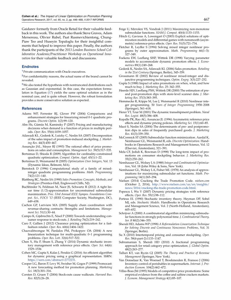
Cohen et al.: The Impact of Linear Optimization on Promotion PlanningOperations Research, 2017, vol. 65, no. 2, pp. 446–468, ©2017 INFORMS 467
Gaidarev formerly from Oracle Retail for their valuable feed-back in this work. The authors also thank SteveGraves, AdamMersereau, Olivier Rubel, Paat Rusmevichientong, Chung-Piaw Teo and Huseyin Topaloglu for their insightful com-ments that helped to improve this paper. Finally, the authorsthank the participants of the 2013 London Business School Col-laborative Academic/Practitioner Workshop on Operational Inno-vation for their valuable feedback and discussions.
Endnotes1Private communication with Oracle executives.2For confidentiality reasons, the actual name of the brand cannot berevealed.3We also tested the hypothesis with nontruncated distributions suchas Gaussian and exponential. In this case, the expectation formu-lation in Equation (17) yields the same optimal solution as in thenominal case, and is quite robust. However, the robust formulationprovides a more conservative solution as expected.
ReferencesAdams WP, Forrester RJ, Glover FW (2004) Comparisons and
enhancement strategies for linearizing mixed 0-1 quadratic pro-grams. Discrete Optim. 1(2):99–120.
Ahn Hs, Gümüs M, Kaminsky P (2007) Pricing and manufacturingdecisions when demand is a function of prices in multiple peri-ods. Oper. Res. 55(6):1039–1057.
Ailawadi KL, Gedenk K, Lutzky C, Neslin SA (2007) Decompositionof the sales impact of promotion-induced stockpiling. J. Market-ing Res. 44(3):450–467.
Assunção JAL, Meyer RJ (1993) The rational effect of price promo-tions on sales and consumption. Management Sci. 39(5):517–535.
Bertsimas D, Shioda R (2009) Algorithm for cardinality-constrainedquadratic optimization. Comput. Optim. Appl. 43(1):1–22.
Bertsimas D, Weismantel R (2005) Optimization Over Integers, Vol. 13(Dynamic Ideas, Belmont, MA).
Bienstock D (1996) Computational study of a family of mixed-integer quadratic programming problems. Math. Programming74(2):121–140.
Blattberg RC, Neslin SA (1990) Sales Promotion: Concepts, Methods, andStrategies (Prentice-Hall, Englewood Cliffs, NJ).
Buchbinder N, Feldman M, Naor JS, Schwartz R (2012) A tight lin-ear time (1/2)-approximation for unconstrained submodularmaximization. Proc. 53rd Annual IEEE Sympos. Foundations Com-put. Sci., FOCS ’12 (IEEE Computer Society, Washington, DC),649–658.
Cachon GP, Lariviere MA (2005) Supply chain coordination withrevenue-sharing contracts: Strengths and limitations. Manage-ment Sci. 51(1):30–44.
Campo K, Gijsbrechts E, Nisol P (2000) Towards understanding con-sumer response to stock-outs. J. Retailing 76(2):219–242.
Caro F, Gallien J (2012) Clearance pricing optimization for a fast-fashion retailer. Oper. Res. 60(6):1404–1422.
Chaovalitwongse W, Pardalos PM, Prokopyev OA (2004) A newlinearization technique for multi-quadratic 0–1 programmingproblems. Oper. Res. Lett. 32(6):517–522.
Chen X, Hu P, Shum S, Zhang Y (2014) Dynamic stochastic inven-tory management with reference price effects. Oper. Sci. 64(6):1529–1536
Cohen MC, Gupta S, Kalas J, Perakis G (2016) An efficient algorithmfor dynamic pricing using a graphical representation. SSRN:https://ssrn.com/abstract�2772231.
Cooper LG, Baron P, Levy W, Swisher M, Gogos P (1999) Promocast:A new forecasting method for promotion planning. MarketingSci. 18(3):301–316.
Corsten D, Gruen T (2004) Stock-outs cause walkouts. Harvard Bus.Rev. 82(5):26–28.
Feige U, Mirrokni VS, Vondrak J (2011) Maximizing non-monotonesubmodular functions. SIAM J. Comput. 40(4):1133–1153.
Fibich G, Gavious A, Lowengart O (2003) Explicit solutions of opti-mizationmodels and differential gameswith nonsmooth (asym-metric) reference-price effects. Oper. Res. 51(5):721–734.
Fletcher R, Leyffer S (1994) Solving mixed integer nonlinear pro-grams by outer approximation. Math. Programming 66(1–3):327–349.
Foekens EW, Leeflang SHP, Wittink DR (1998) Varying parametermodels to accommodate dynamic promotion effects. J. Econo-metrics 89(1):249–268.
Gedenk K, Neslin SA, Ailawadi KL (2006) Sales promotion. Retailingin the 21st Century (Springer, Berlin), 345–359.
Grossmann IE (2002) Review of nonlinear mixed-integer and dis-junctive programming techniques. Optim. Engrg. 3(3):227–252.
Gupta S (1988) Impact of sales promotions on when, what, and howmuch to buy. J. Marketing Res. 25: 342–355.
Heerde HJV, Leeflang PSH, Wittink DR (2000) The estimation of pre-and post-promotion dips with store-level scanner data. J. Mar-keting Res. 37(3):383–395.
Hemmecke R, Köppe M, Lee J, Weismantel R (2010) Nonlinear inte-ger programming. 50 Years of Integer Programming 1958–2008(Springer), 561–618.
Herer YT, Tzur M (2001) The dynamic transshipment problem.NavalRes. Logist. 48(5):386–408.
Kopalle PK, Rao AG, Assuncao JL (1996) Asymmetric reference priceeffects and dynamic pricing policies.Marketing Sci. 15(1):60–85.
Macé S, Neslin SA (2004) The determinants of pre- and postpromo-tion dips in sales of frequently purchased goods. J. MarketingRes. 41(3):339–350.
McCormick ST (2005) Submodular function minimization. Aardal K,Nemhauser GL, Weismantel R, eds.Discrete Optimization.Hand-books in Operations Research and Management Science, Vol. 12(Elsevier, Amsterdam), 321–391.
Mela CF, Jedidi K, Bowman D (1998) The long-term impact of pro-motions on consumer stockpiling behavior. J. Marketing Res.35(2):250–262.
Nemhauser GL,Wolsey LA (1988) Integer and Combinatorial Optimiza-tion, Vol. 18 (John Wiley & Sons, New York).
Nemhauser GL, Wolsey LA, Fisher ML (1978) An analysis of approx-imations for maximizing submodular set functions. Math. Pro-gramming 14(1):265–294.
Nielsen (2014) Cracking the Trade Promotion Code. nielsen.com(October 2, 2014), http://www.nielsen.com/us/en/insights/news/2014/cracking-the-trade-promotion-code.html.
Popescu I, Wu Y (2007) Dynamic pricing strategies with referenceeffects. Oper. Res. 55(1):98–112.
Porteus EL (1990) Stochastic inventory theory. Heyman DP, SobelMJ, eds. Stochastic Models. Handbooks in Operations Researchand Management Science, Vol. 2 (North-Holland, Amsterdam),605–652.
Schrijver A (2000) A combinatorial algorithm minimizing submodu-lar functions in strongly polynomial time. J. Combinatorial Theory,Ser. B 80(2):346–355.
Sherali HD, AdamsWP (1998)AReformulation-Linearization Techniquefor Solving Discrete and Continuous Nonconvex Problems, Vol. 31(Springer, Berlin).
Su X (2010) Intertemporal pricing and consumer stockpiling. Oper.Res. 58(4-part-2):1133–1147.
Subramanian S, Sherali HD (2010) A fractional programmingapproach for retail category price optimization. J. Global Optim.48(2):263–277.
Talluri KT, van Ryzin GJ (2005) The Theory and Practice of RevenueManagement (Springer, New York).
Van Donselaar K, Van Woensel T, Broekmeulen R, Fransoo J (2006)Inventory control of perishables in supermarkets. Internat. J. Pro-duction Econom. 104(2):462–472.
Villas-Boas JM (1995) Models of competitive price promotions: Someempirical evidence from the coffee and saltine crackers markets.J. Econom. Management Strategy 4(1):85–107.

Cohen et al.: The Impact of Linear Optimization on Promotion Planning468 Operations Research, 2017, vol. 65, no. 2, pp. 446–468, ©2017 INFORMS
Zhao W, Zheng YS (2000) Optimal dynamic pricing for perishableassets with nonhomogeneous demand. Management Sci. 46(3):375–388.
Maxime C. Cohen is an assistant professor of informa-tion, operations and management sciences at Stern School ofBusiness, New York University. His research lies at the inter-section of data analytics and operations management. He isinterested in pricing applications such as retail, sustainabil-ity, airline, and cloud services.
Ngai-Hang Zachary Leung is an assistant professor inthe Department of Management Sciences at the College ofBusiness of the City University of Hong Kong. His currentresearch interests include inventory management, revenuemanagement, and healthcare operations.
Kiran Panchamgam is a principal scientist in the Retail Sci-ence R&Dgroup at Oracle Inc, Burlington,MA.He has strongexpertise (and also pending patents) in developing analyticalsolutions using data mining, machine learning, econometricand optimization techniques for business problems in retail.
Georgia Perakis is the William F. Pounds Professor ofManagement at the Sloan School of Management, Mas-sachusetts Institute of Technology and is group head of theOperationsManagement group atMIT Sloan. In her research,she investigates how analytics can benefit complex real-worldproblems in pricing, revenue management, supply chain,energy and transportation applications. Perakis has receivedthe CAREER Award from the NSF and the PECASE Awardfrom the Office of the President on Science and Technology.She was recently elected as INFORMS Fellow, a recognitionfor lifetime contributions to the field.
Anthony Smith is Vice President of Science Services atRevionics, which provides price, markdown, and promotionoptimization solutions for the retail industry. He has 30 yearsof experience in advanced analytic and science-based soft-ware, and for the past 12 years, has focused on retail data sci-ence and analytics, including demand forecasting, price opti-mization, supply chain and replenishment, and assortmentspace optimization. He holds anMS ECE from the Universityof Massachusetts, Amherst.