The Impact of Income Inequality on Individual Happiness: Evidence from China

The Impact of Income Inequality on IndividualHappiness: Evidence from China

Peng Wang • Jay Pan • Zhehui Luo

Accepted: 7 May 2014� Springer Science+Business Media Dordrecht 2014

Abstract Using survey data from China, this paper tests the association between indi-

vidual self-reported happiness and income inequality. The hypothesized relationship

between income inequality and individual happiness is an inverted-U shaped association

based on the tunnel effect theory proposed by Hirschman and Rothschild (Q J Econ

87(4):544–566, 1973). Using the Chinese General Social Survey data, we empirically

investigate the relationship between income inequality and individual happiness and we

find evidence confirming the tunnel effect hypothesis. Specifically, individual happiness

increases with inequality when county-level inequality measured by the Gini coefficient is

less than 0.405, and decreases with inequality for larger values of the Gini coefficient,

where approximately 60 % of the counties in the study have a Gini coefficient larger than

0.405. The inverted U-shaped association exists in both urban and rural China; however,

the turning points for urban and rural areas are 0.323 and 0.459, respectively. Between the

rich and poor groups, the inverted-U shape relationship exists only in the poor subsample.

Keywords Income inequality � Happiness � Subjective wellbeing � China

Everything we do we do to ensure that the people live a happier life with more

dignity and to make our society fairer and more harmonious.

P. WangSchool of Economics, Southwest University for Nationalities, Chengdu, Chinae-mail: [email protected]

J. Pan (&)West China School of Public Health, Sichuan University, Chengdu, Chinae-mail: [email protected]

J. PanWest China Research Center for Rural Health Development, Sichuan University, Chengdu, China

Z. LuoDepartment of Epidemiology and Biostatistics, Michigan State University, East Lansing, MI, USA

123

Soc Indic ResDOI 10.1007/s11205-014-0651-5

- Delivered by Premier of the State Council of China (Wen Jiabao) at the Third

Session of the Eleventh National People’s Congress on March 5, 2010.

1 Introduction

The recent rapid economic growth of the Chinese economy is accompanied by a marked

increase in income inequality. The Gini coefficient increased from 0.293 in 1978, to 0.372

in 2000, and to 0.474 in 2012 (Kanbur and Zhang 2005; National Bureau of Statistics of

China 2013). Based on available data from the World Bank (2013); out of 154 countries,

only 53 countries have higher Gini coefficients than China.

The rising income inequality of China may produce serious social and economic

problems. Income inequality might slow economic growth (Aghion et al. 1999; Benjamin

et al. 2006), cause frequent social conflicts (Alesina and Perotti 1996), lead to higher levels

of violent crime (Hsieh and Pugh 1993), reduce social trust (Jordahl 2007; Rothstein and

Uslaner 2005), and harm the health of the citizens (Asafu-Adjaye 2004; Li and Zhu 2006).

While inequality may affect society and its economic development in many ways, this

paper focuses on a more integral part of the socio-economic effects of inequality, the

impact of income inequality on individual happiness.

Happiness, or subjective wellbeing, is a person’s cognitive and affective evaluation of

his or her own life (Diener et al. 2009). Happiness is an important comprehensive index of

the quality of individual and social life. Job security, social status and power, pecuniary

rewards, and even good health are desirable not for the goods per se but for the satisfaction

and happiness afforded through these things (Frey and Stutzer 2002).

Although there is a large body of research on income ineqaulity and happiness, few

researchers have investigated the relationship in developing countries, especially China.

The limited existing research on this relationship has focused exclusively on the linear

effect of income inequality on happiness. In contrast, the tunnel effect hypothesis, pro-

posed by Hirschman and Rothschild (1973), states that happiness rises with income

inequality when inequality is low; however, happiness decreases once income inequality

continues to increase after reaching a certain threshold. In this study, we test the nonlinear

relationship between income ineqaulity and happiness in China and estimate the threshold

where the relationship between happiness and income inequality changes direction, if the

tunnel effect hypothesis is confirmed.

The structure of the paper is as follows: Sect. 2 provides a brief review of the literature

on the relationship between happiness and income inequality, Sect. 3 describes the data and

presents our methodology, and Sect. 4 summarizes the results of empirical analyses,

conclusions, and policy implications.

2 Literature Review

This paper studies the impact of income inequality on individual happiness by focusing on

the economic literature that utilizes large-scale survey data regarding happiness.

Empirical evidence on the sign and significance of the relationship between income

inequality and happiness is widely disputed amongst economic literature. Some studies

have found a negative correlation between income inequality and happiness. The first

contribution, Morawetz et al. (1977), compares the self-rated happiness of the citizens of

P. Wang et al.

123

two neighboring communities in Israel that have different levels of income inequality, with

the conclusion that higher levels of income inequality lead to lower average self-rated

happiness. Using aggregated data of eight nations over a 25 year period, Hagerty (2000)

shows that a decrease of the skewness, or the inequality, of the income distribution for a

country increases its average national happiness. Alesina et al. (2004) discover the negative

effects on happiness due to income inequality in Europe and the United States. Graham and

Felton (2006) use survey data from 18 countries in Latin America and ascertain that

income inequality, as an indicator of persistent unfairness, has a negative effect on hap-

piness. Schwarze and Harpfer (2007), using the German Socio-Economic Panel Study data

find that German people are negatively affected by income inequality. Using a compiled

dataset from the European and the World Values surveys from 1981 to 2004, Verme (2011)

finds that income inequality has a negative and significant effect on life satisfaction. Their

result is robust to changes of explanatory variables and estimation choices, persisting

across different income groups and across different types of countries. Oishi et al. (2011)

find that Americans, on average, are happier in years with less national income inequality

than in years with greater inequality. Oshio and Kobayashi (2011) also find that individuals

who reside in areas of high income inequality in Japan tend to self-report less happiness.

In contrast, some studies have indicated a positive association between income

inequality and happiness. Tomes (1986) uses survey data from Canada and finds that self-

reported happiness is lower when the share of income going to the poorest 40 % of a

community is larger, holding personal characteristics constant. Using the British House-

hold Panel Survey data, Clark and Delta (2003) similarly discover that a positive corre-

lation exists between happiness and inequality measured by either the Gini coefficient or

the 90th/10th income percentile ratio for the employed population. Ohtake and Tomioka

(2004) find that both the Gini coefficient and perception of rising income inequality have a

weak but positive correlation to happiness in Japan.

Other researchers have found no relationship between happiness and income inequality.

Helliwell (2003) presents no evidence that income inequality is correlated with subjective

well-being. Using panel data from the Russian Longitudinal Monitoring Survey, Senik

(2004) finds that neither national level inequality nor regional inequality has a significant

effect on reported life satisfaction. Berg and Veenhoven (2010) use a dataset involved 119

nations during the period 2000–2006, and find little relation between income inequality and

the average happiness of its citizens.

Only a few studies on income inequality and happiness have been conducted in China,

with mixed conclusions. Smyth and Qian (2008) find persons who perceive income dis-

tribution as unequal report lower levels of happiness in urban China, with differing results

between high and low income individuals. Knight et al. (2009) study the determinants of

happiness among Chinese rural residents and finds that an increase in the Gini coefficient at

the county level increases the happiness of peasants, attributing the results to a ‘‘demon-

stration effect’’ of income inequality. Jiang et al. (2012) find that people feel unhappy with

between-group income inequality;1 however, city-level Gini coefficients in China are

positively correlated with happiness.

Empirical studies regarding income inequality and happiness reach conflicting con-

clusions. Different results are supported by different theories that can lead to the prediction

of either a negative or a positive impact of income inequality on happiness.

1 They measure ‘‘between-group inequality’’ by the income gap between migrants without local hukou andurban residents.

The Impact of Income Inequality on Individual Happiness

123

First, there is an assumption that aversion to inequality is an intrinsic social preference

(Bolton and Ockenfels 2000; Fehr and Schmidt 1999; Kahneman and Krueger 2006).

Recently, Tricomi et al. (2010) use functional magnetic resonance imaging to directly test

for the existence of inequality-averse social preferences in the human brain. The results

show that the brain’s reward circuitry is sensitive to both inequalities of advantageous and

disadvantageous natures. The inequality-averse social preference indicates that higher

income inequality is associated with lower level of happiness.

Second, Runciman (1966) proposes a social justice theory based on the notion of an

individual’s sense of deprivation. Relative deprivation is the feeling of being deprived of

an individual’s perceived entitlement (Walker and Smith 2002). It refers to the discon-

tentment people feel when they compare their positions to others and realize that they have

less (Bayertz 1999). Yitzhaki (1979) applies this concept to income and proposes a

measure of relative deprivation as the sum of the distances of a person’s income from all

higher incomes in a given income distribution, and this measure is shown to be equivalent

to the absolute Gini coefficient. The Runciman and Yitzhaki framework states that

increasing income inequality increases relative deprivation and thus decreases happiness.

On the other hand, Hirschman and Rothschild (1973) argue that people may appreciate

inequality if it signals social mobility, a phenomenon also called the ‘‘tunnel effect’’. They

use an analogy to explain: I am driving through a two-lane tunnel with both lanes running

the same direction; however, I run into a traffic jam with cars stopped in both lanes for as

far as the eye can see. I am in the left lane and feel dejected; however, after a few minutes

the cars in the right lane begins to move. Naturally, my spirits are lifted considerably, for I

know that the traffic jam has been broken and the left lane will begin to move shortly Even

though I sit still, I feel better than before because I am expecting to begin moving soon.

Suppose that after a while, the right lane continues moving while the left lane is still

stopped, in which case I, along with all the other left lane drivers suspect foul play and

many of the left lane drivers will become discontent and take action, such as illegally

crossing the double line, in order to correct the injustice that they feel has been placed upon

them.

Analogously, people who observe that others around themselves move upwards in the

income ladder would increase their expectations about their own income in the future.

Therefore, inequality makes them happier because inequality improves a person’s

expectations about their own future. Hence, people accept and tolerate income inequality

within reasonable limits for some time, but after the limits are reached, reactions turn

negative. This theory attempts to explain the mechanisms regarding how income

inequality affects individual happiness. In reality, the findings from empirical studies are

often the results of compound effects originating from different mechanisms. Some

theories during a certain period of time or in a certain country are more prominent than

other theories.

The happiness effect of inequality for countries transitioning to a market economy such

as China may be different from relatively stable and prosperous countries, such as the

United States. Sanfey and Teksoz (2007) find that income inequality has a positive effect

on life satisfaction in transitioning countries, whereas the impact is negative in stable,

prosperous countries. Grosfeld and Senik (2010) study the changing attitudes toward

inequality during the transition to a market economy in Poland. By using repeated cross-

sections of the population, they find a negative association between inequality and hap-

piness for the second half of the transition period (1997–2005); however, they find a

positive association in the early years of transition (1992–1996).

P. Wang et al.

123

In recent years China is in its most important period of reform, a transition to a market-

oriented economy. Meanwhile, along with the break of the traditional mode of egalitarian

income distribution, China sets up a new distribution mode that allows some people and

regions to get rich first, when and where conditions permit. Persons and regions with faster

economic development can help promote the progress of persons and regions with slower

development, or can set an example to motivate the lagging ones to work harder. Thus,

income inequality improves production enthusiasm, promotes economic development, and

enhances the overall happiness of people. In other words, the ‘‘positive tunnel effect’’ of

proper income inequality on happiness may exist in China. On the other hand, the ‘‘neg-

ative tunnel effect’’ could also exist in China. Due to historically relatively equal distri-

butions of income and wealth, the Chinese people are unlikely to tolerate an increase in

income inequality, which can bring many social problems that could hinder economic

development, interfere with people’s lives, and eventually lead to the reduction of an

individual’s level of happiness.

Based on previous literature, we propose the core hypothesis of our study: income

inequality increases happiness when inequality is low and decreases happiness when

inequality crosses a certain threshold; specifically, the relationship between happiness and

income inequality may follow an inverted-U shape and conform to the ‘‘tunnel effect’’

theory.

3 Data and Estimation

3.1 Data

The data used in this study are from the China General Social Survey (CGSS), jointly

conducted by the Department of Sociology at Renmin University of China and the Survey

Research Centre of Hong Kong University of Science and Technology in September and

October, 2006, with the goal of understanding the quality of life for Chinese citizens. The

survey utilizes a four-phase (county, town, village and household) stratified sampling

design for the collection of data for a nationally representative sample of Chinese citizens.

The samples of the first three phases were identified under the sampling frame of China’s

Fifth National Population Census and families were randomly selected within the selected

villages or neighborhood committees (Hu et al. 2011). Overall, 10,151 households from

969 villages (neighborhood committees), 236 towns (streets), 125 counties (districts), and

28 provinces (municipalities)2 were selected for a face-to-face interview. The CGSS

collects a wide range of socio-demographic indicators, such as gender, marriage, age,

education, employment, income, and household size in addition to information on hap-

piness. The sample is restricted to respondents aged between 18 and 70 that were not

missing information on key demographic variables such as age, income, and gender. After

cleaning the data for the data analysis, a final sample size of 8,208 observations was

chosen. Table 1 (Column 2) summarizes the definitions and their descriptive statistics for

the key variables in our final sample.

2 In total, China has 31 provinces, municipalities, and autonomous regions in mainland China. Qinghai,Ningxia, and Tibet were not covered in this survey, because the population of the three regions onlyaccounts for a very small proportion of the whole nation, missing them should not affect the nationalrepresentativeness of the survey.


123

3.1.1 Happiness Indicator

The outcome variable in our study is the happiness score of the household respondent,

obtained from a multiple-choice question: ‘‘Taken all together, how happy are you at

present?’’ The five possible responses to the question are ‘‘not happy at all’’, ‘‘not happy’’,

‘‘so–so’’, ‘‘happy’’, and ‘‘very happy’’. Happiness is the most widely used indicator in the

related literature (Ferrer-i-Carbonell and Frijters 2004; Knight and Gunatilaka 2010;

Knight et al. 2009; Tomioka and Ohtake 2004). Veenhoven (1996) reviews findings on

validity and reliability, concluding that single item measures on subjective wellbeing are

akin to muli-item inventories, providing sufficiently validity and reliability as a happiness

measurement. For our analysis, we construct an ordinal variable ‘‘Happiness’’ with a value

ranging from 1 to 5, corresponding to ‘‘not happy at all’’, ‘‘not happy’’, ‘‘so–so’’, ‘‘happy’’,

and ‘‘very happy’’, respectively.

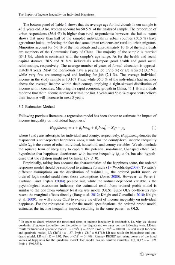
The column (1) of Table 2 reports the sample summary statistics concerning happiness

status. Among all individuals, more than 45 % reported being happy or very happy while

less than 8 % of respondents perceive their situation as not happy or not happy at all.

Examining the data by gender and rural/urban status in Table 2, we find that men are

slightly less happy than women, with 7.92 % of men but only 7.36 % of women self-

reporting a lack of happiness. By contrast, the rural/urban disparity in happiness seems to

be larger with 46.62 % of urban residents self-reporting themselves to be ‘‘very happy’’ or

‘‘happy’’, compared with 44.22 % for rural residents.

3.1.2 Income Inequality Measures

The survey includes several inequality measures as shown in Table 1. The Gini coefficient

is the main inequality measure we will use. The county is the basic unit of local gov-

ernment and administration in China (Knight et al. 2009); therefore, the Gini coefficient is

based on county-level individual income. Since China has 125 counties, or districts, that

are included in our sample, there are 125 distinct income inequality indexes. Table 1 shows

that the Gini coefficient within the counties ranges from 0.194 to 0.662, with an average of

0.428. The Gini coefficient also shows that there is larger income inequality in rural

counties than in urban counties in China.

Several other inequality measures are also created for data analysis and comparison,

including the Theil index and the income share of the richest 50 %. For consistency with

the Gini, we group individual income within the same county to generate these inequality

indicators. Unlike the Gini and income share of the richest 50 %, which ranges between 0

and 1, the Theil index is continuous. For concise presentation of our results, we use the

Gini for main analysis and other measures for the robustness test.

3.1.3 Other Explanatory Variables

Subjective happiness is determined by many factors. Following the literature (for example,

Argyle 1999; Frey and Stutzer 2002; Alesina et al. 2004; Dolan et al. 2008; Smyth and

Qian 2008; Knight et al. 2009; Jiang et al. 2012), a set of variables, including individual

and household characteristics, was added in the regression model to control for potential

confounding factors. We utilize the log of annual individual income and relative income to

control for the influence of household income on happiness. Since the expectation of future

income is an important determinant of current happiness (Luo 2006; Knight et al. 2009;

Knight and Gunatilaka 2010), dummy variables indicating anticipated income levels for

P. Wang et al.

123

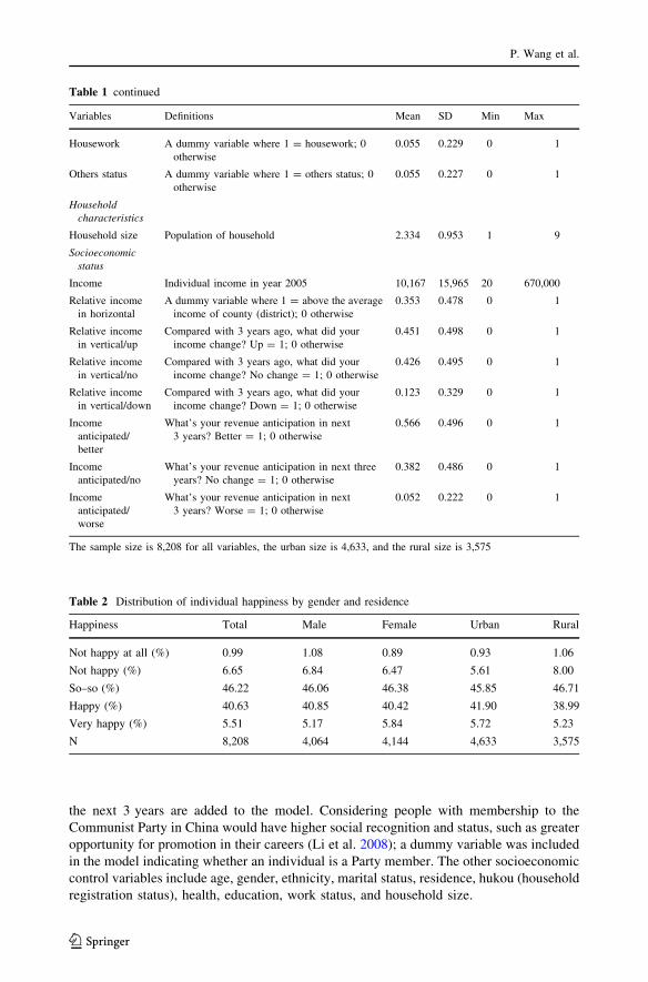
Table 1 Sample summary statistics

Variables Definitions Mean SD Min Max

Happiness status

Happiness 1 = ‘‘not happy at all’’; 2 = ‘‘not happy’’;

3 = ‘‘so–so’’; 4 = ‘‘happy’’; 5 = ‘‘very

happy’’

3.430 0.740 1 5

Income inequality

Gini coefficient Gini coefficient of income within the county 0.428 0.082 0.194 0.662

Gini coefficient in

urban

Gini coefficient of income within the county in

urban subsample

0.378 0.072 0.194 0.687

Gini coefficient in

rural

Gini coefficient of income within the county in

rural subsample

0.445 0.082 0.246 0.667

Theil index Theil index of income within the county 0.348 0.155 0.064 1.123

Inc50 % Income share of the richest 50 % within the

county

0.792 0.053 0.629 0.932

Individual

characteristics

Age Age of the respondent in years 43.205 12.895 18 70

Gender A dummy variable where 1 = female; 0 = male 0.505 0.500 0 1

Residence A dummy variable where 1 = urban; 0 = rural 0.564 0.496 0 1

Hukou A dummy variable where 1 = non-agricultural;

0 = agricultural

0.495 0.500 0 1

Ethnicity A dummy variable where 1 = minority;

0 = Han

0.066 0.248 0 1

Political status A dummy variable where 1 = member of

communist party of China; 0 otherwise

0.098 0.297 0 1

Marital status:

single

A dummy variable where 1 = single; 0

otherwise

0.100 0.300 0 1

Marital status:

married

A dummy variable where 1 = married; 0

otherwise

0.841 0.366 0 1

Marital status:

other

A dummy variable where 1 = other marital

status; 0 single or married

0.060 0.237 0 1

Human capital

Health A dummy variable where 1 = rather or very

good; 0 otherwise

0.785 0.411 0 1

Education Years of education received from school 8.086 4.198 0 22

Social capital

Relationship A dummy variable where 1 = rather or very

good; 0 otherwise

0.918 0.274 0 1

Work status

Paid work A dummy variable where 1 = paid work; 0

otherwise

0.726 0.446 0 1

Never work and

looking for a job

A dummy variable where 1 = never work and

looking for a job; 0 otherwise

0.004 0.059 0 1

Unemployed and

looking for a job

A dummy variable where 1 = Unemployed and

looking for a job; 0 otherwise

0.021 0.143 0 1

Student or

military

A dummy variable where 1 = student or

military; 0 otherwise

0.007 0.085 0 1

Retired A dummy variable where 1 = retired; 0

otherwise

0.132 0.339 0 1


123

the next 3 years are added to the model. Considering people with membership to the

Communist Party in China would have higher social recognition and status, such as greater

opportunity for promotion in their careers (Li et al. 2008); a dummy variable was included

in the model indicating whether an individual is a Party member. The other socioeconomic

control variables include age, gender, ethnicity, marital status, residence, hukou (household

registration status), health, education, work status, and household size.

Table 1 continued

Variables Definitions Mean SD Min Max

Housework A dummy variable where 1 = housework; 0

otherwise

0.055 0.229 0 1

Others status A dummy variable where 1 = others status; 0

otherwise

0.055 0.227 0 1

Household

characteristics

Household size Population of household 2.334 0.953 1 9

Socioeconomic

status

Income Individual income in year 2005 10,167 15,965 20 670,000

Relative income

in horizontal

A dummy variable where 1 = above the average

income of county (district); 0 otherwise

0.353 0.478 0 1

Relative income

in vertical/up

Compared with 3 years ago, what did your

income change? Up = 1; 0 otherwise

0.451 0.498 0 1

Relative income

in vertical/no


income change? No change = 1; 0 otherwise

0.426 0.495 0 1

Relative income

in vertical/down


income change? Down = 1; 0 otherwise

0.123 0.329 0 1

Income

anticipated/

better

What’s your revenue anticipation in next

3 years? Better = 1; 0 otherwise

0.566 0.496 0 1

Income

anticipated/no

What’s your revenue anticipation in next three

years? No change = 1; 0 otherwise

0.382 0.486 0 1

Income

anticipated/

worse

What’s your revenue anticipation in next

3 years? Worse = 1; 0 otherwise

0.052 0.222 0 1

The sample size is 8,208 for all variables, the urban size is 4,633, and the rural size is 3,575

Table 2 Distribution of individual happiness by gender and residence

Happiness Total Male Female Urban Rural

Not happy at all (%) 0.99 1.08 0.89 0.93 1.06

Not happy (%) 6.65 6.84 6.47 5.61 8.00

So–so (%) 46.22 46.06 46.38 45.85 46.71

Happy (%) 40.63 40.85 40.42 41.90 38.99

Very happy (%) 5.51 5.17 5.84 5.72 5.23

N 8,208 4,064 4,144 4,633 3,575

P. Wang et al.

123

The bottom panel of Table 1 shows that the average age for individuals in our sample is

43.2 years old. Also, women account for 50.5 % of the analyzed sample. The proportion of

urban respondents (56.4 %) is higher than rural respondents; however, the hukou status

shows that more than half of the sampled individuals in urban counties (50.5 %) have

agriculture hukou, reflecting the fact that some urban residents are rural-to-urban migrants.

Minorities account for 6.6 % of the individuals and approximately 10 % of the individuals

are members of the Communist Party of China. The majority of the sample is married

(84.1 %), which is consistent with the sample’s age range. As for the health and social

capital statuses, 78.5 and 91.8 % individuals self-report good health and good social

relationships, respectively. The average number of years of formal education is approxi-

mately 8 years. Most the individuals have a paying job (72.6 %) or are retired (13.2 %);

while very few are unemployed and looking for job (2.1 %). The average individual

income in the study sample is 10,167 Yuan, while 35.3 % of the individuals had incomes

above the average income within their county, implying a right-skewed distribution of

income within counties. Mirroring the rapid economic growth in China, 45.1 % individuals

reported that their income increased within the last 3 years and 56.6 % respondents believe

their income will increase in next 3 years.

3.2 Estimation Method

Following previous literature, a regression model has been chosen to estimate the impact of

income inequality on individual happiness:3

Happinessij ¼ aþ b1Ineqj þ b2Ineq2j þ Xijcþ lij ð1Þ

where i and j are subscripts for individual and county, respectively. Happinessij denotes the

respondent’s self-reported happiness. Ineqj stands for the county-level income inequality

while Xij is the vector of other individual, household, and county variables. We also include

the squared term of inequality to capture the potential non-linear, U-shaped effect. We

hypothsize that happiness deteriorates with income inequality (b1 [ 0), but also hypoth-

esize that the relation might not be linear (b2 = 0).

Empirically, taking into account the characteristics of the happiness score, the ordered

responses model should be employed to estimate formula (1) (Wooldridge2009). To satisfy

different assumptions on the distribution of residual lij, the ordered probit model or

ordered logit model could meet those assumptions (Jones 2000). However, as Ferrer-i-

Carbonell and Frijters (2004) pointed out, while the ordinal dependent variable is the

psychological assessment indicator, the estimated result from ordered probit model is

similar to the one from ordinary least squares model (OLS). Since OLS coefficients rep-

resent the marginal effects directly (Jiang et al. 2012; Knight and Gunatilaka 2010; Knight

et al. 2009), we will choose OLS to explore the effect of income inequality on individual

happiness. For the robustness test for the model specifications, the ordered probit model

estimates the income inequality impact, resulting in the same pattern as OLS.

3 In order to check whether the functional form of income inequality is reasonable, i.e. why we choosequadratic of income inequality, not the cubic or the biquadrate, we carry out the following tests. LR-testresult for linear and quadratic model: LR Chi2(1) = 22.62, Prob [ Chi2 = 0.0000; LR-test result for cubicand quadratic model: LR Chi2(1) = 1.87, Prob [ Chi2 = 0.1712; LR-test result for biquadrate and qua-dratic model: LR chi2(1) = 3.92, Prob [ Chi2 = 0.1408; Ramsey RESET test using powers of the fittedvalues of happiness for the quadratic model, Ho: model has no omitted variables, F(3, 8,173) = 1.09,Prob [ F=0.3534.


123

4 Results

4.1 The Impact of Income Inequality on Happiness

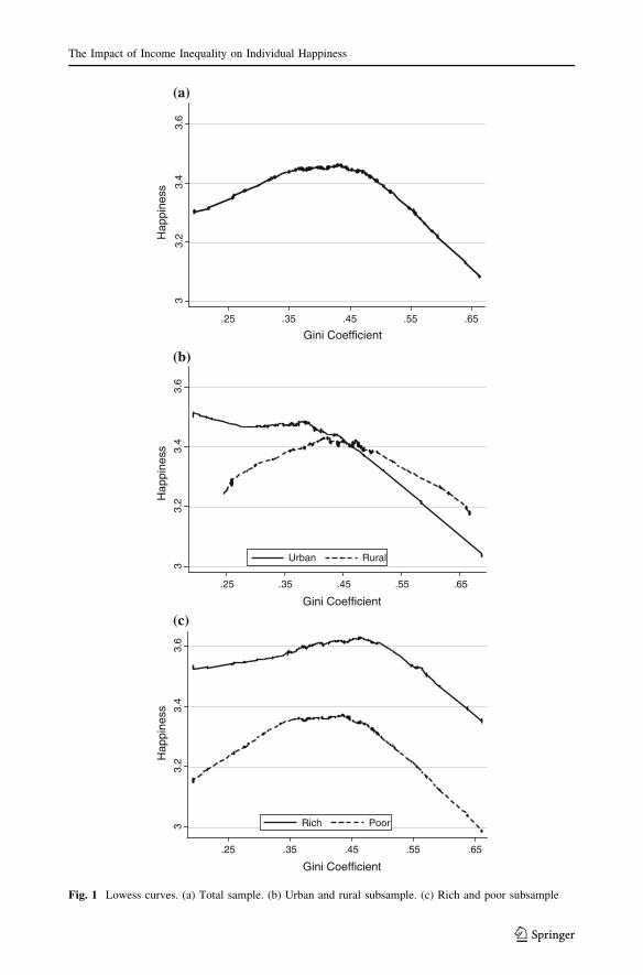
Lowess curves (Cleveland 1979) are used to examine the relationship between happiness

and income inequality for total sample, the rural/urban subgroup, and the rich/poor sub-

group. Although the curves are unadjusted for control variables and few observations are

present at very high and low values of the Gini, Fig. 1 illustrates important features on the

relationship between individual happiness and income inequality. Among the total sample

(Fig. 1a), happiness directly increases with the Gini until the Gini reaches a value between

0.42 and 0.44. Above a Gini between 0.42 and 0.44, the happiness decreases as inequality

increases. Compared to rural counties (Fig. 1b), the urban curve reaches the maximum at a

lower Gini coefficient, somewhere between 0.38 and 0.39. A respondent is classified as

rich if their income is above the average income in their county; otherwise, the respondent

is classified as poor. Although rich individuals are found to be happier on average than

poor individuals, both curves reach a maximum with a Gini in between 0.42 and 0.44, after

which happiness gradually declines (Fig. 1c).

In short, all Lowess curves in Fig. 1 show that the happiness first increases and then

decreases at different rates after reaching their respective maximums with the increase of

the Gini coefficient, thus we describe the curves as inverted-U shaped relationships

between happiness and income inequality, coinciding with our original hypothesis of a

nonlinear relationship between happiness and income inequality.

The OLS regression method is then implemented to control for other variables that

affect individual happiness in order to better understand the partial effect of income

inequality on happiness. Table 3 presents the estimation results.4 With further support for

our hypothesis in Fig. 1, the regression results also exhibit the inverted-U shaped (a

quadratic relationship) between happiness and the Gini.

For comparison with existing literature, the Gini squared term is not included in Column

(1). The coefficient of the Gini is negative and significant at the 10 % significance level,

with all other potential confounding variables controlled for. When we add the squared

term in Column (2), the coefficients of the Gini and Gini squared are both significant at the

1 % significance level. The positive coefficient of the Gini and negative coefficient of Gini

squared indicate an inverted-U shaped relationship between the Gini and happiness.

Specifically, happiness increases with inequality when the Gini coefficient is less than

0.4055 and decreases with income inequality for larger Gini coefficient. In the study

sample 59.2 % of the counties have Gini values higher than 0.405, which corresponds to

60 % of study subjects living in high income inequality counties.

Rather than relying on a single measure of income inequality such as the Gini coeffi-

cient, we also chose two other indicators to test; the Theil index and the income share of

the richest 50 %, for a robustness test, and columns (3) and (4) in Table 3 report their

respective estimations. The results present further consistent evidence for an inverted-U

association between happiness and income inequality. The peak of happiness is at 0.291 for

the Theil index, where 60 % of the sample counties have higher inequality than this turning

4 Addressing the potential heteroskedasticity of the error term, we report the robust standard errors for allthe regression. In fact, we have also estimated the standard errors and find the results are similar.5 The formula: turning point for Gini = -[effect of Gini/(2�effect of Gini2)], that is, the Gini at the peak ofthe inverted U-shaped curve of Gini and happiness.

P. Wang et al.

123

33.

23.

43.

6

Hap

pine

ss

.25 .35 .45 .55 .65

Gini Coefficient

(a)

33.

23.

43.

6

Hap

pine

ss

.25 .35 .45 .55 .65

Gini Coefficient

Urban Rural

(b)

33.

23.

43.

6

Hap

pine

ss

.25 .35 .45 .55 .65

Gini Coefficient

Rich Poor

(c)

Fig. 1 Lowess curves. (a) Total sample. (b) Urban and rural subsample. (c) Rich and poor subsample


123

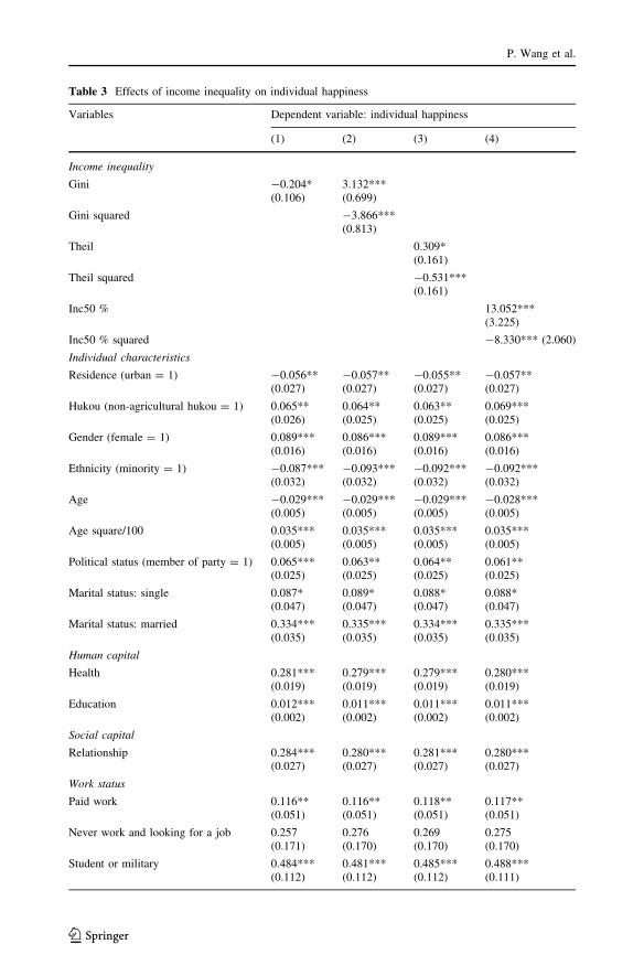
Table 3 Effects of income inequality on individual happiness

Variables Dependent variable: individual happiness

(1) (2) (3) (4)

Income inequality

Gini -0.204*(0.106)

3.132***(0.699)

Gini squared -3.866***(0.813)

Theil 0.309*(0.161)

Theil squared -0.531***(0.161)

Inc50 % 13.052***(3.225)

Inc50 % squared -8.330*** (2.060)

Individual characteristics

Residence (urban = 1) -0.056**(0.027)

-0.057**(0.027)

-0.055**(0.027)

-0.057**(0.027)

Hukou (non-agricultural hukou = 1) 0.065**(0.026)

0.064**(0.025)

0.063**(0.025)

0.069***(0.025)

Gender (female = 1) 0.089***(0.016)

0.086***(0.016)

0.089***(0.016)

0.086***(0.016)

Ethnicity (minority = 1) -0.087***(0.032)

-0.093***(0.032)

-0.092***(0.032)

-0.092***(0.032)

Age -0.029***(0.005)

-0.029***(0.005)

-0.029***(0.005)

-0.028***(0.005)

Age square/100 0.035***(0.005)

0.035***(0.005)

0.035***(0.005)

0.035***(0.005)

Political status (member of party = 1) 0.065***(0.025)

0.063**(0.025)

0.064**(0.025)

0.061**(0.025)

Marital status: single 0.087*(0.047)

0.089*(0.047)

0.088*(0.047)

0.088*(0.047)

Marital status: married 0.334***(0.035)

0.335***(0.035)

0.334***(0.035)

0.335***(0.035)

Human capital

Health 0.281***(0.019)

0.279***(0.019)

0.279***(0.019)

0.280***(0.019)

Education 0.012***(0.002)

0.011***(0.002)

0.011***(0.002)

0.011***(0.002)

Social capital

Relationship 0.284***(0.027)

0.280***(0.027)

0.281***(0.027)

0.280***(0.027)

Work status

Paid work 0.116**(0.051)

0.116**(0.051)

0.118**(0.051)

0.117**(0.051)

Never work and looking for a job 0.257(0.171)

0.276(0.170)

0.269(0.170)

0.275(0.170)

Student or military 0.484***(0.112)

0.481***(0.112)

0.485***(0.112)

0.488***(0.111)

P. Wang et al.

123

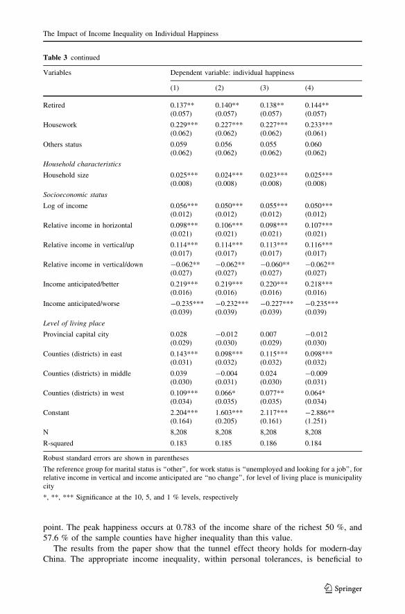
point. The peak happiness occurs at 0.783 of the income share of the richest 50 %, and

57.6 % of the sample counties have higher inequality than this value.

The results from the paper show that the tunnel effect theory holds for modern-day

China. The appropriate income inequality, within personal tolerances, is beneficial to

Table 3 continued


(1) (2) (3) (4)

Retired 0.137**(0.057)

0.140**(0.057)

0.138**(0.057)

0.144**(0.057)

Housework 0.229***(0.062)

0.227***(0.062)

0.227***(0.062)

0.233***(0.061)

Others status 0.059(0.062)

0.056(0.062)

0.055(0.062)

0.060(0.062)

Household characteristics

Household size 0.025***(0.008)

0.024***(0.008)

0.023***(0.008)

0.025***(0.008)

Socioeconomic status

Log of income 0.056***(0.012)

0.050***(0.012)

0.055***(0.012)

0.050***(0.012)

Relative income in horizontal 0.098***(0.021)

0.106***(0.021)

0.098***(0.021)

0.107***(0.021)

Relative income in vertical/up 0.114***(0.017)

0.114***(0.017)

0.113***(0.017)

0.116***(0.017)

Relative income in vertical/down -0.062**(0.027)

-0.062**(0.027)

-0.060**(0.027)

-0.062**(0.027)

Income anticipated/better 0.219***(0.016)

0.219***(0.016)

0.220***(0.016)

0.218***(0.016)

Income anticipated/worse -0.235***(0.039)

-0.232***(0.039)

-0.227***(0.039)

-0.235***(0.039)

Level of living place

Provincial capital city 0.028(0.029)

-0.012(0.030)

0.007(0.029)

-0.012(0.030)

Counties (districts) in east 0.143***(0.031)

0.098***(0.032)

0.115***(0.032)

0.098***(0.032)

Counties (districts) in middle 0.039(0.030)

-0.004(0.031)

0.024(0.030)

-0.009(0.031)

Counties (districts) in west 0.109***(0.034)

0.066*(0.035)

0.077**(0.035)

0.064*(0.034)

Constant 2.204***(0.164)

1.603***(0.205)

2.117***(0.161)

-2.886**(1.251)

N 8,208 8,208 8,208 8,208

R-squared 0.183 0.185 0.186 0.184

Robust standard errors are shown in parentheses

The reference group for marital status is ‘‘other’’, for work status is ‘‘unemployed and looking for a job’’, forrelative income in vertical and income anticipated are ‘‘no change’’, for level of living place is municipalitycity

*, **, *** Significance at the 10, 5, and 1 % levels, respectively


123

individual happiness; however, excessive income inequality weakens individual happiness.

Our explanation for the results is that appropriate levels of income inequality can enhance

income mobility, since income mobility has an egalitarian nature. In an era of rapid

economic development with a certain degree of income inequality, strong motivation to

obtain more wealth is highly stimulated by society as a whole, especially for the middle

and lower class income earners. High expectations accompanied by enhanced confidence

for the future lead to greater individual life satisfaction when faced with income inequality

within their personal tolerances. Within personal tolerances, people believe that income

inequality provides the opportunity for individuals to decrease poverty and that an indi-

vidual can also achieve wealth growth through their own efforts, rather than relying on

their social relationships, the background of their family, and other factors. With a certain

degree of income inequality, people expect that their future opportunities will place them at

a higher level of income distribution. So in this case, income inequality makes a positive

impact to an individual’s subjective happiness, with the positive tunnel effect playing a

major role. However, when the income inequality passes the individual tolerance level of

people for inequality, middle and lower class income earners lose confidence for the future,

and aversion to inequality and relative deprivation would become more prominent, ulti-

mately leading to a negative effect on happiness. Simultaneously, facing higher income

inequality, upper class income earners may worry about the loss of their fortune, resulting

in their decreased individual happiness.

Compared with other empirical results in previous studies on happiness in China

(Knight and Gunatilaka 2010; Knight et al. 2009), our results largely confirm known

correlations with happiness. Compared with rural residents, people with non-agricultural

hukou are happier since household registration is a social status symbol to some extent in

China. Individuals with non-agricultural hukou would enjoy more generous social security,

such as pension insurance (Wang 2006). Females, the Han ethnic group, and communists

also have higher happiness scores. Age has a U-shaped effect on happiness, with a turning

point at 40.7 years of age. Compared with other marital status; including separation,

divorce, and widowed, married persons enjoy family life and have higher happiness scores.

Also, health and education have a positive, significant effect on happiness. People with

better social relationships are happier. Compared with the unemployed, individuals with

paid employment tend have higher self-reported happiness. An interesting finding with

regards to work status is that students, military members, retired persons, and individuals

occupied with full-time housework all have a higher degree of overall happiness than

unemployed individuals. Since family members are able to provide more support for each

other in bigger households, the bigger the size of household, the happier individuals in the

household are. In short, all analyzed socioeconomic status variables have a positive sig-

nificant impact on individual happiness score.

The proposed hypothesis is supported by the results of our empirical analyses and is

robust to other common measurements of inequality. The complete tunnel effect theory is

applicable in China, stating that increasing income inequality improves happiness within a

certain range of inequality, but the effects of higher income inequality become detrimental

to happiness.

4.2 Robustness Checks

According to Oshio and Kobayashi (2011), there is a danger for over-controlling due to the

introduction of too many predictors at the individual level. There is easiness in reporting

findings or failing to identify important associations because there is difficulty in assessing

P. Wang et al.

123

the dynamics between individual-level variables and county-level income inequality. In

addition, there is no well-established theory regarding which control variables matter and

should be included in a model.

Hence, we examine the sensitivity of our results to changes in control variables.

Concretely, we control for two key attributes: individual characteristics including resi-

dence, hukou, gender, ethnicity, age, political status, and marital status in addition to

socioeconomic status characteristics which includes the logarithm of income, relative

income in horizontal, relative income in vertical and anticipated income. We also select

additional variables with other attributes: household characteristics including household

size, human capital referring to both education and health, social capital through rela-

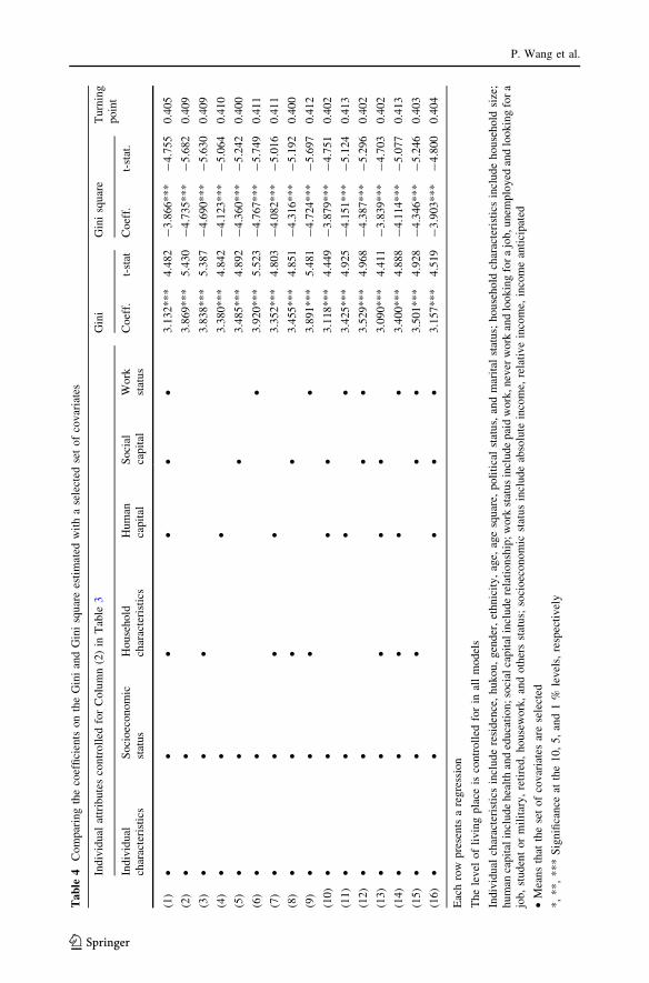
tionships, and work status. Table 4 shows how Gini and Gini squared are affected by the

choice of individual and household controls. The 1 % significantly positive and negative

coefficients of Gini and Gini squared are found in all models. Further, we find that the

turning point varies from 0.400 to 0.413, which is relatively narrow. Our findings dem-

onstrate that the inverted-U shaped relationship between income inequality and happiness

is robust.

Moreover, for the robustness test of the model specifications, the ordered probit and

logit models are also employed to estimate the impact of income inequality. The results,

although not shown in this paper, demonstrate that OLS and second order model have

similar results.

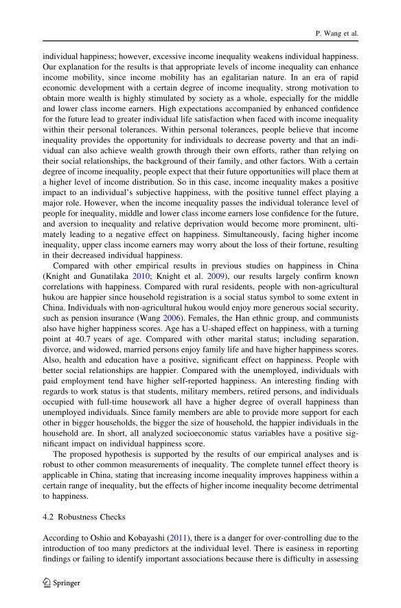
4.3 Subsample Analysis

Considering the tremendous differences in many aspects between urban and rural living

conditions, we further examine the effects of income inequality in rural and urban areas

separately. In addition, the relationship between happiness and income inequality among

the rich and the poor is also examined separately. The subsample results are shown in

Table 5.

As presented in Column (1) and (2) in Table 5, all the coefficients of inequality and

inequality squared variables are significant at the 5 % significance level. The inverted-U

shape relationship between happiness and income inequality occurs for both urban and

rural residents; however, the tolerance of urban residents for income inequality is lower

than rural residents; as shown by the urban internal turning point at 0.323, while the turning

point for rural counties is 0.459. Column (3) and (4) in Table 5 present the results for poor

and rich group individuals, respectively. Income inequality still has an inverted-U shaped

effect on the happiness of the poor; however, the same relationship does not exist for the

rich. In the early stages of China’s economic reform, opening up is ‘‘to allow some regions

and some people to get rich first, and the rich will help underdeveloped regions and the

poor, eventually achieving common prosperity’’. After decades of development, urban and

coastal areas are relatively rich while income inequality widens. Compared to urban res-

idents, rural residents have a lower level of education, limited literacy, higher enthusiasm

for the call of government, and a stronger sense in obedience to law and morality. Rural

residents believe that someone would help them get rich and therefore, they are more

tolerant of income inequality while urban residents tend to view the income inequality as

unfair and are less tolerant of income inequality.

Other interesting findings are shown in Table 5. The impacts of hukou on happiness are

different in urban and rural areas; in urban areas, hukou have a statistically significant

positive coefficient, an indication that urban residents with non-agricultural hukou are

happier than individuals with agricultural hukou. However, there is no significant


123

Ta

ble

4C

om

par

ing

the

coef

fici

ents

on

the

Gin

ian

dG

ini

squ

are

esti

mat

edw

ith

ase

lect

edse

to

fco

var

iate

s

Ind

ivid

ual

attr

ibu

tes

con

tro

lled

for

Co

lum

n(2

)in

Tab

le3

Gin

iG

ini

squ

are

Tu

rnin

gp

oin

tIn

div

idu

alch

arac

teri

stic

sS

oci

oec

on

om

icst

atu

sH

ou

seho

ldch

arac

teri

stic

sH

um

anca

pit

alS

oci

alca

pit

alW

ork

stat

us

Co

eff.

t-st

atC

oef

f.t-

stat

.

(1)

••

••

••

3.1

32

**

*4

.482

-3

.866

**

*-

4.7

55

0.4

05

(2)

••

3.8

69

**

*5

.430

-4

.735

**

*-

5.6

82

0.4

09

(3)

••

•3

.838

**

*5

.387

-4

.690

**

*-

5.6

30

0.4

09

(4)

••

•3

.380

**

*4

.842

-4

.123

**

*-

5.0

64

0.4

10

(5)

••

•3

.485

**

*4

.892

-4

.360

**

*-

5.2

42

0.4

00

(6)

••

•3

.920

**

*5

.523

-4

.767

**

*-

5.7

49

0.4

11

(7)

••

••

3.3

52

**

*4

.803

-4

.082

**

*-

5.0

16

0.4

11

(8)

••

••

3.4

55

**

*4

.851

-4

.316

**

*-

5.1

92

0.4

00

(9)

••

••

3.8

91

**

*5

.481

-4

.724

**

*-

5.6

97

0.4

12

(10

)•

••

•3

.118

**

*4

.449

-3

.879

**

*-

4.7

51

0.4

02

(11

)•

••

•3

.425

**

*4

.925

-4

.151

**

*-

5.1

24

0.4

13

(12

)•

••

•3

.529

**

*4

.968

-4

.387

**

*-

5.2

96

0.4

02

(13

)•

••

••

3.0

90

**

*4

.411

-3

.839

**

*-

4.7

03

0.4

02

(14

)•

••

••

3.4

00

**

*4

.888

-4

.114

**

*-

5.0

77

0.4

13

(15

)•

••

••

3.5

01

**

*4

.928

-4

.346

**

*-

5.2

46

0.4

03

(16

)•

••

••

3.1

57

**

*4

.519

-3

.903

**

*-

4.8

00

0.4

04

Eac

hro

wp

rese

nts

are

gre

ssio

n

Th

ele

vel

of

liv

ing

pla

ceis

con

tro

lled

for

inal

lm

od

els

Indiv

idual

char

acte

rist

ics

incl

ude

resi

den

ce,

hukou,

gen

der

,et

hnic

ity,

age,

age

squar

e,poli

tica

lst

atus,

and

mar

ital

stat

us;

house

hold

char

acte

rist

ics

incl

ude

house

hold

size

;h

um

anca

pit

alin

clu

de

hea

lth

and

edu

cati

on

;so

cial

cap

ital

incl

ud

ere

lati

on

ship

;w

ork

stat

us

incl

ud

ep

aid

wo

rk,n

ever

wo

rkan

dlo

ok

ing

for

ajo

b,u

nem

plo

yed

and

loo

kin

gfo

ra

job

,st

ud

ent

or

mil

itar

y,

reti

red

,h

ou

sew

ork

,an

do

ther

sst

atu

s;so

cioec

on

om

icst

atu

sin

clu

de

abso

lute

inco

me,

rela

tiv

ein

com

e,in

com

ean

tici

pat

ed

•M

eans

that

the

set

of

covar

iate

sar

ese

lect

ed

*,

**

,*

**

Sig

nifi

can

ceat

the

10

,5

,an

d1

%le

vel

s,re

spec

tiv

ely

P. Wang et al.

123

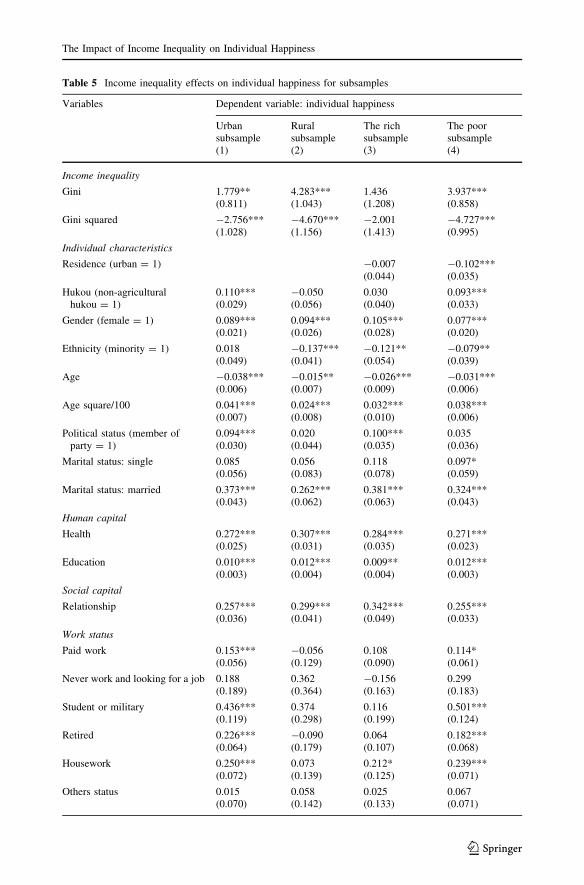
Table 5 Income inequality effects on individual happiness for subsamples


Urbansubsample

Ruralsubsample

The richsubsample

The poorsubsample

(1) (2) (3) (4)

Income inequality

Gini 1.779**(0.811)

4.283***(1.043)

1.436(1.208)

3.937***(0.858)

Gini squared -2.756***(1.028)

-4.670***(1.156)

-2.001(1.413)

-4.727***(0.995)

Individual characteristics

Residence (urban = 1) -0.007(0.044)

-0.102***(0.035)

Hukou (non-agriculturalhukou = 1)

0.110***(0.029)

-0.050(0.056)

0.030(0.040)

0.093***(0.033)

Gender (female = 1) 0.089***(0.021)

0.094***(0.026)

0.105***(0.028)

0.077***(0.020)

Ethnicity (minority = 1) 0.018(0.049)

-0.137***(0.041)

-0.121**(0.054)

-0.079**(0.039)

Age -0.038***(0.006)

-0.015**(0.007)

-0.026***(0.009)

-0.031***(0.006)

Age square/100 0.041***(0.007)

0.024***(0.008)

0.032***(0.010)

0.038***(0.006)

Political status (member ofparty = 1)

0.094***(0.030)

0.020(0.044)

0.100***(0.035)

0.035(0.036)

Marital status: single 0.085(0.056)

0.056(0.083)

0.118(0.078)

0.097*(0.059)

Marital status: married 0.373***(0.043)

0.262***(0.062)

0.381***(0.063)

0.324***(0.043)

Human capital

Health 0.272***(0.025)

0.307***(0.031)

0.284***(0.035)

0.271***(0.023)

Education 0.010***(0.003)

0.012***(0.004)

0.009**(0.004)

0.012***(0.003)

Social capital

Relationship 0.257***(0.036)

0.299***(0.041)

0.342***(0.049)

0.255***(0.033)

Work status

Paid work 0.153***(0.056)

-0.056(0.129)

0.108(0.090)

0.114*(0.061)

Never work and looking for a job 0.188(0.189)

0.362(0.364)

-0.156(0.163)

0.299(0.183)

Student or military 0.436***(0.119)

0.374(0.298)

0.116(0.199)

0.501***(0.124)

Retired 0.226***(0.064)

-0.090(0.179)

0.064(0.107)

0.182***(0.068)

Housework 0.250***(0.072)

0.073(0.139)

0.212*(0.125)

0.239***(0.071)

Others status 0.015(0.070)

0.058(0.142)

0.025(0.133)

0.067(0.071)


123

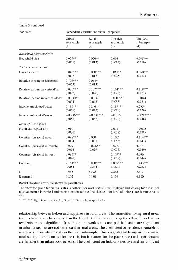
relationship between hokou and happiness in rural areas. The minorities living rural areas

tend to have lower happiness than the Han, but differences among the ethnicities of urban

residents are not significant. In addition, the work status and political status are significant

in urban areas, but are not significant in rural areas. The coefficient on residence variable is

negative and significant only in the poor subsample. This suggests that living in an urban or

rural setting doesn’t matter for the rich, but it matters for the poor since rural poor persons

are happier than urban poor persons. The coefficient on hukou is positive and insignificant

Table 5 continued


Urbansubsample

Ruralsubsample

The richsubsample

The poorsubsample

(1) (2) (3) (4)

Household characteristics

Household size 0.027**(0.011)

0.026**(0.012)

0.006(0.014)

0.035***(0.010)

Socioeconomic status

Log of income 0.046***(0.017)

0.080***(0.017)

0.061**(0.025)

0.050***(0.014)

Relative income in horizontal 0.108***(0.027)

0.064*(0.035)

– –

Relative income in vertical/up 0.086***(0.022)

0.137***(0.026)

0.104***(0.028)

0.118***(0.021)

Relative income in vertical/down -0.080**(0.034)

-0.032(0.043)

-0.108**(0.053)

-0.044(0.031)

Income anticipated/better 0.195***(0.021)

0.246***(0.025)

0.189***(0.028)

0.235***(0.020)

Income anticipated/worse -0.236***(0.051)

-0.230***(0.062)

-0.056(0.072)

-0.283***(0.046)

Level of living place

Provincial capital city 0.010(0.031)

0.011(0.052)

-0.013(0.038)

Counties (districts) in east 0.098***(0.034)

0.050(0.031)

0.100*(0.055)

0.114***(0.041)

Counties (districts) in middle 0.029(0.034)

-0.065**(0.029)

-0.003(0.053)

0.014(0.040)

Counties (districts) in west 0.095**(0.041)

– 0.119**(0.059)

0.056(0.044)

Constant 2.161***(0.254)

0.880***(0.334)

1.878***(0.370)

1.483***(0.253)

N 4,633 3,575 2,895 5,313

R-squared 0.202 0.180 0.136 0.180


The reference group for marital status is ‘‘other’’, for work status is ‘‘unemployed and looking for a job’’, forrelative income in vertical and income anticipated are ‘‘no change’’, for level of living place is municipalitycity


P. Wang et al.

123

for the rich while it is significant for the poor. The poor with non-agricultural hukou have a

higher happiness level than the poor with agricultural hukou.

4.4 Cross-Level Effects

When aggregated data are used along with individual data, a hierarchical structure of

multilevel data exists and macroeconomic inequality indicators may affect individual

variables; commonly referred to as the cross-level effect. Income inequality may affect

happiness through individual characteristics since different people have different attitudes

and perceptions of income inequality. Next, we examine whether a cross-level effect of

income inequality exists by including a series of interactions between individual charac-

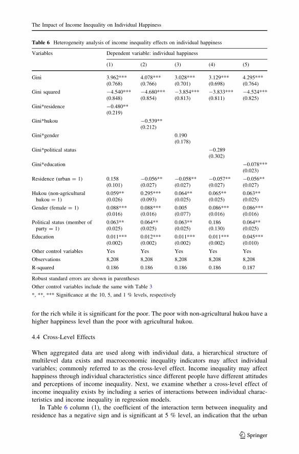
teristics and income inequality in regression models.

In Table 6 column (1), the coefficient of the interaction term between inequality and

residence has a negative sign and is significant at 5 % level, an indication that the urban

Table 6 Heterogeneity analysis of income inequality effects on individual happiness


(1) (2) (3) (4) (5)

Gini 3.962***(0.768)

4.078***(0.766)

3.028***(0.701)

3.129***(0.698)

4.295***(0.764)

Gini squared -4.540***(0.848)

-4.680***(0.854)

-3.854***(0.813)

-3.833***(0.811)

-4.524***(0.825)

Gini*residence -0.480**(0.219)

Gini*hukou -0.539**(0.212)

Gini*gender 0.190(0.178)

Gini*political status -0.289(0.302)

Gini*education -0.078***(0.023)

Residence (urban = 1) 0.158(0.101)

-0.056**(0.027)

-0.058**(0.027)

-0.057**(0.027)

-0.056**(0.027)

Hukou (non-agriculturalhukou = 1)

0.059**(0.026)

0.295***(0.093)

0.064**(0.025)

0.065**(0.025)

0.063**(0.025)

Gender (female = 1) 0.088***(0.016)

0.088***(0.016)

0.005(0.077)

0.086***(0.016)

0.086***(0.016)

Political status (member ofparty = 1)

0.063**(0.025)

0.064**(0.025)

0.063**(0.025)

0.186(0.130)

0.064**(0.025)

Education 0.011***(0.002)

0.012***(0.002)

0.011***(0.002)

0.011***(0.002)

0.045***(0.010)

Other control variables Yes Yes Yes Yes Yes

Observations 8,208 8,208 8,208 8,208 8,208

R-squared 0.186 0.186 0.186 0.186 0.187


Other control variables include the same with Table 3



123

residents dislike income inequality more than rural residents. This demonstrates that urban

residents have less happiness on average because of the acute reaction to income inequality

for urban residents, i.e. the low tolerance of income inequality. In Column (2), the inter-

action term of household hukou and inequality is added, and the result is similar with

Column (1) indicating that people with non-agricultural identity dislike income inequality

more than people with agricultural hukou. We separately specify additional interaction

terms for income inequality with gender and political status in Column (3) and (4),

respectively, but neither of the interactions demonstrates statistical significance at 10 %, an

indication of no difference in the perception of income inequality between women and

men, or between party members and non-party members. When the interaction between

income inequality and education, there is a statistically negative cross-level effect, which

means that individuals with higher levels of education dislike income inequality more than

less educated individuals, likely explained by data that shows that people with higher

education typically earn a higher income.

5 Conclusion

This paper focuses on the effect of income inequality on individual happiness. Prior

theoretical and empirical work has supported positive, negative, or insignificant associa-

tions. With China in a critical period of reform and economic transformation, we

hypothesize that the relationship between income inequality and happiness in China

exhibits an inverted-U shape based on the ‘‘tunnel effect’’ theory, a theory that states that

happiness increases with income inequality when inequality is low; however happiness

subsequently decreases when inequality crosses a certain threshold. The Chinese General

Social Survey data is employed to test the inverted-U shape hypothesis.

Our empirical results support the inverted-U shaped association between income

inequality and happiness, confirming the ‘‘tunnel effect’’ theory exists in China. Overall,

individual happiness increases with income inequality when the county-level Gini coef-

ficient is less than 0.405 and decreases with inequality for larger county-level Gini coef-

ficients. About 59 % of the counties, or districts, have a Gini coefficient higher than 0.405.

The robustness of the findings is checked, with special attention to other measures for

income inequality and the specifications of the control variables. All estimates of the

effects of income inequality on happiness in China are consistent across different income

inequality measures and model specifications.

Rural/urban and poor/rich subsamples are also analyzed to explore the heterogeneous

effect of income inequality in different groups. The ‘‘inverted-U’’ associations still exist in

urban and rural China with the urban residents’ tolerance for income inequality at a lower

level than rural residents since the turning point for urban residents is 0.323, while it is

0.459 for rural residents.

Furthermore, considering income inequality may affect happiness through individual

characteristics, five interaction terms are added to regressions to study the cross-level

effects of income inequality. We find that people living in urban counties, people with non-

agricultural hukou, and people with higher education are less happy than their respective

counterparts at the same level of income inequality.

Currently, the Party Central Committee and the People’s Government of China pay

unprecedented attention to the wellbeing of its citizens, fully committed to ‘‘building a

socialist harmonious society’’ and our empirical results are informative for Chinese policy

makers. Income inequality does not necessarily harm social welfare; however, lower levels

P. Wang et al.

123

of income inequality are associated with a higher happiness level. On the one hand, income

inequality stimulates an individual‘s desire to improve their living decisions, but on the

other hand, high levels of income inequality might hurt morale and raise social unrest.

Keeping income inequality within reasonable bounds, rather than completely eliminating

income inequality, is a more reasonable policy response.

The study has two limitations. First, the measurement of individual happiness uses a

single item and is based on the survey results of a subjective assessment. Although hap-

piness is a complex and multi-dimensional concept, one overall score provides a simple

and easy interpretation for analyses. If one truly wishes to elucidate aspects of happiness

affected by income inequality, measurements with better psychometric properties would

benefit analysis. Second, we do not investigate the relationship between happiness and

income inequality over time due to a current lack of time series data. Further research is

needed to address this issue in the future.

Acknowledgments This study was funded by the Applied Economics Research Funds of SouthwestUniversity for Nationalities (2011XWD-S0202), the National Natural Science Foundation of China(71303165), Sichuan University (skqx201401), the China Postdoctoral Science Foundation (2013M540706)and China Medical Board (13-167). We are grateful to the seminar and conference participants at South-western University of Finance and Economics for their insightful comments, and to colleagues at the PKUCenter of Health Economics Research, Gordon G. Liu, Gergely Horvath and the anonymous referees. Dataanalyzed in this paper were collected by the research project ‘‘China General Social Survey (CGSS)’’sponsored by the China Social Science Foundation. This research project was carried out by Department ofSociology, Renmin University of China and Social Science Division, Hong Kong Science and TechnologyUniversity, and directed by Dr. Li Lulu and Dr. Bian Yanjie. The authors appreciate the assistance inproviding data by the institutes and individuals aforementioned. The authors are responsible for allremaining errors.

References

Aghion, P., Caroli, E., & Garcia-Penalosa, C. (1999). Inequality and economic growth: The perspective ofthe new growth theories. Journal of Economic Literature, 37(4), 1615–1660.

Alesina, A., Di Tella, R., & MacCulloch, R. (2004). Inequality and happiness: Are Europeans and Amer-icans different? Journal of Public Economics, 88(9), 2009–2042.

Alesina, A., & Perotti, R. (1996). Income distribution, political instability, and investment. EuropeanEconomic Review, 40(6), 1203–1228.

Argyle, M. (1999). Causes and correlates of happiness. In Daniel Kahneman, Ed Diener, & Norbert Schwarz(Eds.), Well-being: The foundations of hedonic psychology (pp. 353–373). New York: Russell SageFoundation.

Asafu-Adjaye, J. (2004). Income inequality and health: A multi-country analysis. International Journal ofSocial Economics, 31(1/2), 195–207.

Bayertz, K. (1999). Solidarity. Berlin: Springer.Benjamin, D., Brandt, L., & Giles, J. (2006). Inequality and growth in rural China: Does higher inequality

impede growth?: IZA discussion papers.Berg, M., & Veenhoven, R. (2010). Income inequality and happiness in 119 nations. Erasmus University

Rotterdam, Faculty of Social Sciences. Working papers.Bolton, G. E., & Ockenfels, A. (2000). ERC: A theory of equity, reciprocity, and competition. American

economic review, 90(1), 166–193.Clark, A., & Delta. (2003). Inequality-aversion and Income Mobility: A direct test. Delta.Cleveland, W. S. (1979). Robust locally weighted regression and smoothing scatterplots. Journal of the

American Statistical Association, 74(368), 829–836.Diener, E., Oishi, S., & Lucas, R. E. (2009). Subjective Well-Being: The Science of Happiness and Life

Satisfaction. In C.R. Snyder & Shane J. Lopez (Eds.), The Oxford handbook of positive psychology (pp.187–194). Oxford: Oxford University Press.


123

Dolan, P., Peasgood, T., & White, M. (2008). Do we really know what makes us happy? A review of theeconomic literature on the factors associated with subjective well-being. Journal of Economic Psy-chology, 29(1), 94–122.

Fehr, E., & Schmidt, K. M. (1999). A theory of fairness, competition, and cooperation. The QuarterlyJournal of Economics, 114(3), 817–868.

Ferrer-i-Carbonell, A., & Frijters, P. (2004). How important is methodology for the estimates of thedeterminants of happiness? The Economic Journal, 114(497), 641–659.

Frey, B. S., & Stutzer, A. (2002). What can economists learn from happiness research? Journal of EconomicLiterature, 40(2), 402–435.

Graham, C., & Felton, A. (2006). Inequality and happiness: Insights from Latin America. The Journal ofEconomic Inequality, 4(1), 107–122.

Grosfeld, I., & Senik, C. (2010). The emerging aversion to inequality. Economics of Transition, 18(1), 1–26.Hagerty, M. R. (2000). Social comparisons of income in one’s community: Evidence from national surveys

of income and happiness. Journal of Personality and Social Psychology, 78(4), 764.Helliwell, J. F. (2003). How’s life? Combining individual and national variables to explain subjective well-

being. Economic Modelling, 20(2), 331–360.Hirschman, A. O., & Rothschild, M. (1973). The changing tolerance for income inequality in the course of economic

development with a mathematical appendix. The Quarterly Journal of Economics, 87(4), 544–566.Hsieh, C–. C., & Pugh, M. D. (1993). Poverty, income inequality, and violent crime: A meta-analysis of

recent aggregate data studies. Criminal Justice Review, 18(2), 182–202.Hu, F., Xu, Z., & Chen, Y. (2011). Circular migration, or permanent stay? Evidence from China’s rural–

urban migration. China Economic Review, 22(1), 64–74.Jiang, S., Lu, M., & Sato, H. (2012). Identity, inequality, and happiness: Evidence from urban China. World

Development, 40(6), 1190–1200.Jones, A. M. (2000). Health econometrics. Handbook of Health Economics, 1, 265–344.Jordahl, H. (2007). Inequality and trust. Research Institute of Industrial Economics (IFN) working paper,

715.Kahneman, D., & Krueger, A. B. (2006). Developments in the measurement of subjective well-being. The

Journal of Economic Perspectives, 20(1), 3–24.Kanbur, R., & Zhang, X. (2005). Fifty years of regional inequality in China: A journey through central

planning, reform, and openness. Review of Development Economics, 9(1), 87–106.Knight, J., & Gunatilaka, R. (2010). Great expectations? The subjective well-being of rural–urban migrants

in China. World Development, 38(1), 113–124.Knight, J., Song, L., & Gunatilaka, R. (2009). Subjective well-being and its determinants in rural China.

China Economic Review, 20(4), 635–649.Li, H., Meng, L., Wang, Q., & Zhou, L. (2008). Political connections, financing and firm performance:

Evidence from Chinese private firms. Journal of Development Economics, 87(2), 283–299.Li, H., & Zhu, Y. (2006). Income, income inequality, and health: Evidence from China. Journal of Com-

parative Economics, 34(4), 668–693.Luo, C. (2006). Urban-rural division, employment status and subjective well-being. China Economic

Quarterly, 5(3), 817–840. (in Chinese).Morawetz, D., Atia, E., Bin-Nun, G., Felous, L., Gariplerden, Y., Harris, E., et al. (1977). Income distri-

bution and self-rated happiness: Some empirical evidence. The Economic Journal, 87(347), 511–522.National Bureau of Statistics of China (2013). Press conference on national economy of 2012. http://www.

stats.gov.cn/tjgz/tjdt/201301/t20130118_17719.html (in Chinese).Ohtake, F., & Tomioka, J. (2004). Who supports redistribution? Japanese Economic Review, 55(4),

333–354.Oishi, S., Kesebir, S., & Diener, E. (2011). Income inequality and happiness. Psychological Science, 22(9),

1095–1100.Oshio, T., & Kobayashi, M. (2011). Area-level income inequality and individual happiness: Evidence from

Japan. Journal of Happiness Studies, 12(4), 633–649.Rothstein, B., & Uslaner, E. M. (2005). All for all: Equality, corruption, and social trust. World Politics,

58(01), 41–72.Runciman, W. G. (1966). Relative deprivation and social justice: A study of attitudes to social inequality in

twentieth-century England. California: University of California.Sanfey, P., & Teksoz, U. (2007). Does transition make you happy? Economics of Transition, 15(4),

707–731.Schwarze, J., & Harpfer, M. (2007). Are people inequality averse, and do they prefer redistribution by the

state?: Evidence from german longitudinal data on life satisfaction. The Journal of Socio-Economics,36(2), 233–249.

P. Wang et al.

123

http://www.stats.gov.cn/tjgz/tjdt/201301/t20130118_17719.html

http://www.stats.gov.cn/tjgz/tjdt/201301/t20130118_17719.html

Senik, C. (2004). When information dominates comparison: Learning from Russian subjective panel data.Journal of Public Economics, 88(9), 2099–2123.

Smyth, R., & Qian, X. (2008). Inequality and happiness in urban China. Economics Bulletin, 4(23), 1–10.Tomes, N. (1986). Income distribution, happiness and satisfaction: A direct test of the interdependent

preferences model. Journal of Economic Psychology, 7(4), 425–446.Tomioka, J., & Ohtake, F. (2004). Happiness and Income Inequality in Japan. Mimeo: Osaka University.Tricomi, E., Rangel, A., Camerer, C. F., & O’Doherty, J. P. (2010). Neural evidence for inequality-averse

social preferences. Nature, 463(7284), 1089–1091.Veenhoven, R. (1996). Happy life-expectancy. Social Indicators Research, 39(1), 1–58.Verme, P. (2011). Life satisfaction and income inequality. Review of Income and Wealth, 57(1), 111–127.Walker, I., & Smith, H. J. (2002). Relative deprivation: Specification, development, and integration.

Cambridge: Cambridge University Press.Wang, D. (2006). China’s urban and rural old age security system: Challenges and options. China & World

Economy, 14(1), 102–116.Wooldridge, J. M. (2009). Introductory econometrics: A modern approach. South Western, Cengage

Learning.World Bank (2013). World DataBank. http://data.worldbank.org/.Yitzhaki, S. (1979). Relative deprivation and the Gini coefficient. The quarterly journal of economics,

93(2), 321–324.


123

http://data.worldbank.org/

Documents

The Impact of Income Inequality on Individual Happiness: Evidence from China