The Impact of Imports and Exports Performance on the

International Journal of Economics and Finance; Vol. 10, No. 1; 2018

ISSN 1916-971X E-ISSN 1916-9728

Published by Canadian Center of Science and Education

110

The Impact of Imports and Exports Performance on the Economic

Growth of Somalia

Ali Abdulkadir Ali1, Ali Yassin Sheikh Ali

2 & Mohamed Saney Dalmar

3

1 Faculty of Humanities, Somali University, Mogadishu, Somalia

2 Faculty of Economics, SIMAD University, Mogadishu, Somalia

3 Graduate Studies, SIMAD University, Mogadishu, Somalia

Correspondence: Ali Yassin, School of Economics, SIMAD University, Somalia. Tel: 252-61-222-5577. E-mail:

[email protected]

Received: October 16, 2017 Accepted: November 25, 2017 Online Published: December 10, 2017

doi:10.5539/ijef.v10n1p110 URL: https://doi.org/10.5539/ijef.v10n1p110

Abstract

In this paper the impact of exports and imports on the economic growth of Somalia over the period 1970-1991

was investigated. The study applied econometric methods such as Ordinary Least Squares technique. The

Granger Causality and Johansen Co-integration tests were also used for analysing the long term association. By

using Augmented Dickey-Fuller (ADF) and Phillip-Perron (PP) stationarity test, the variables proved to be

integrated of the order one 1(1) at first difference. Johansen test of co-integration was used to determine if there

is a long run association in the variables. To determine the direction of causality among the variables, both in the

long and short run, the Pair-wise Granger Causality test was carried out. It was found that economic growth does

not Granger Cause Export but was found hat export Granger Cause GDP. So this implies that there is

unidirectional causality between exports and economic growth. Also there is bidirectional Granger Causality

between import and export. The results show that economic growth in Somalia requires export-led growth

strategy as well as export led import. Imports and exports are thus seen as the source of economic growth in

Somalia.

Keywords: export, import, economic growth, Somalia

1. Introduction

This economic publication begins by presenting a summary of the evolution of foreign trade theories since the

middle of the 12th century, beginning with the school of naturalists, commercialists, and Adam Smith, as well as

comparative advantages, and ending with the theory of modern trade based on assumptions different from the

previous theories, the most important of which is the monopoly of monopoly competition in international trade;

heterogeneity of goods, rather than their homogeneity; and increased yields with size rather than yield stability.

These lectures also address the definition of the statistical framework of foreign trade data through the balance of

payments, including the definition of the balance structure and accounts and the concept of surplus and deficit.

We then move on to introduce trade policies in the form of import substitution, and associated key instruments

such as nominal and effective protection, exchange rates, quota systems, and their effects on economic

performance. In addition, other studies focus on comparisons of certain policies to export promotion policies and

associated external orientation at the expense of the internal trend of the market. The most important World

Trade organization (WTO) agreements related to the performance of trade policies, such as those related to

tariffs, permissible and prohibited subsidies, MFNs, national treatment, non-tariff restrictions, and intellectual

property rights, are also referred to.

There are many views on the relationship between foreign trade and economic growth. For example, some

classics, like Adam Smith, had an optimistic view of this relationship. Smith referred to the impact of trade in

creating the opportunity to apply specialization, divisions of labour, and surplus production efficiencies.

The Somali state is working on the development of its economy to raise the welfare of its citizens, and in this

context, it has tended in 1980s era towards the implementation of programs of economic reform, increasing the

role of the private sector in the development processes and liberalisation of markets, and internal and external

trade, and in the framework of adaptation to international economic variables and the establishment of the

ijef.ccsenet.org International Journal of Economics and Finance Vol. 10, No. 1; 2018

111

multilateral trading system, includes trade in services in the agricultural and industrial products, textiles and

clothing, and intellectual property rights and trade-related investment measures. Accordingly, these variables

have led to the creation of a new international trading system that aims to liberalize global trade of all tariff and

non-tariff barriers and open markets to exports from all countries. The new world order is based on market

mechanisms and the ability of states to compete in goods at the international level.

The impact of imports and exports on economic growth has been a very popular topic, showing the interest of

academicians and policy-makers. The purpose of this interest is to increase gross domestic production and thus

improve the quality of life of citizens. The current study determines the role of import and export performance

on economic growth in Somalia. Somalia is a country located in the Horn of Africa, with a long coastal area that

had historical trade with ancient civilizations, such as the Egyptians and Middle East countries, as well as the

Portuguese. The country is now recovering from the effects of a long civil war and repeated famine and droughts.

The country’s economy is now in the expansion stage after two and a half decades of conflict.

In the last 25 years of less effective government, the condition of the economy was not good, and international

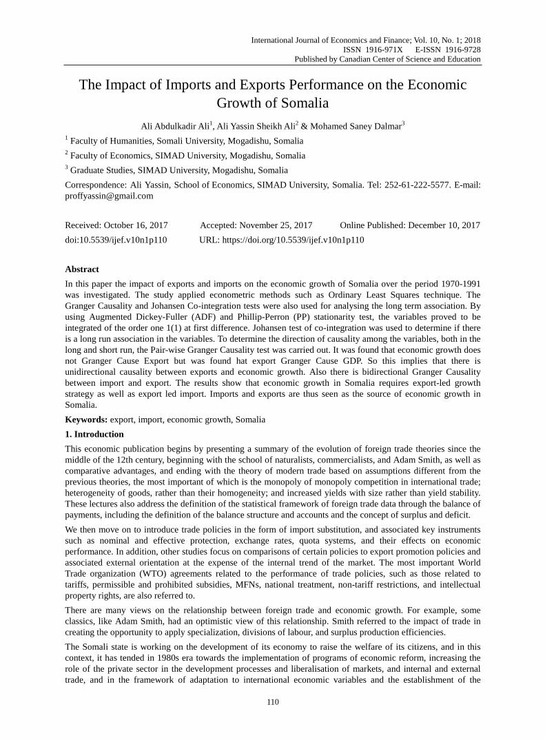
trade was part of those suffering economic sectors. Exports were small, and only livestock played a crucial role,

but it could not stabilise the country’s trade balance account while other sectors did not have a surplus to export

or were idle. However, the economy has been in continuous growth in the last six years, but this did not affect

the country’s role in international markets. The integration of Somalia into international markets is very weak

due to an absence of effective government, lack of banks and financial institutions with international standards,

poor infrastructure, and lack of quality standards and controls to check exported products. Somalia’s main

exports are livestock, including goats, sheep, camel, and cattle; hides and skin; banana; sesame; fish; and

charcoal, with the main export partners being Saudi Arabia, the United Arab Emirates, Oman, Yemen, and Brazil.

Figure 1. Export performance

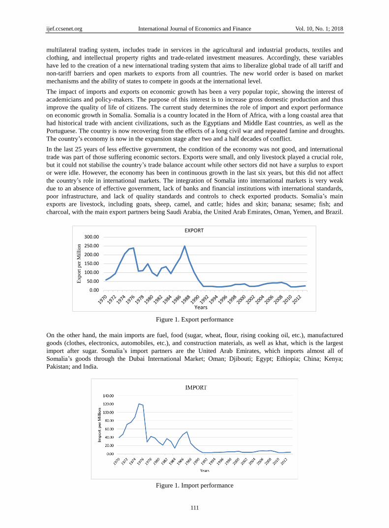
On the other hand, the main imports are fuel, food (sugar, wheat, flour, rising cooking oil, etc.), manufactured

goods (clothes, electronics, automobiles, etc.), and construction materials, as well as khat, which is the largest

import after sugar. Somalia’s import partners are the United Arab Emirates, which imports almost all of

Somalia’s goods through the Dubai International Market; Oman; Djibouti; Egypt; Ethiopia; China; Kenya;

Pakistan; and India.

Figure 1. Import performance

0.00

50.00

100.00

150.00

200.00

250.00

300.00

Exp

ort

per

Mil

lion

Years

EXPORT


112

Imports were larger before the 1990s, especially in the mid-1970s, but were unstable in that period. The

fluctuations seen in Figure 2 show the ups and downs. Imports slowed down after the collapse of the central

government in 1991. Political instability, pirates, weak purchasing power, and lack of government consumption

are key factors that led to decreased Somali imports.

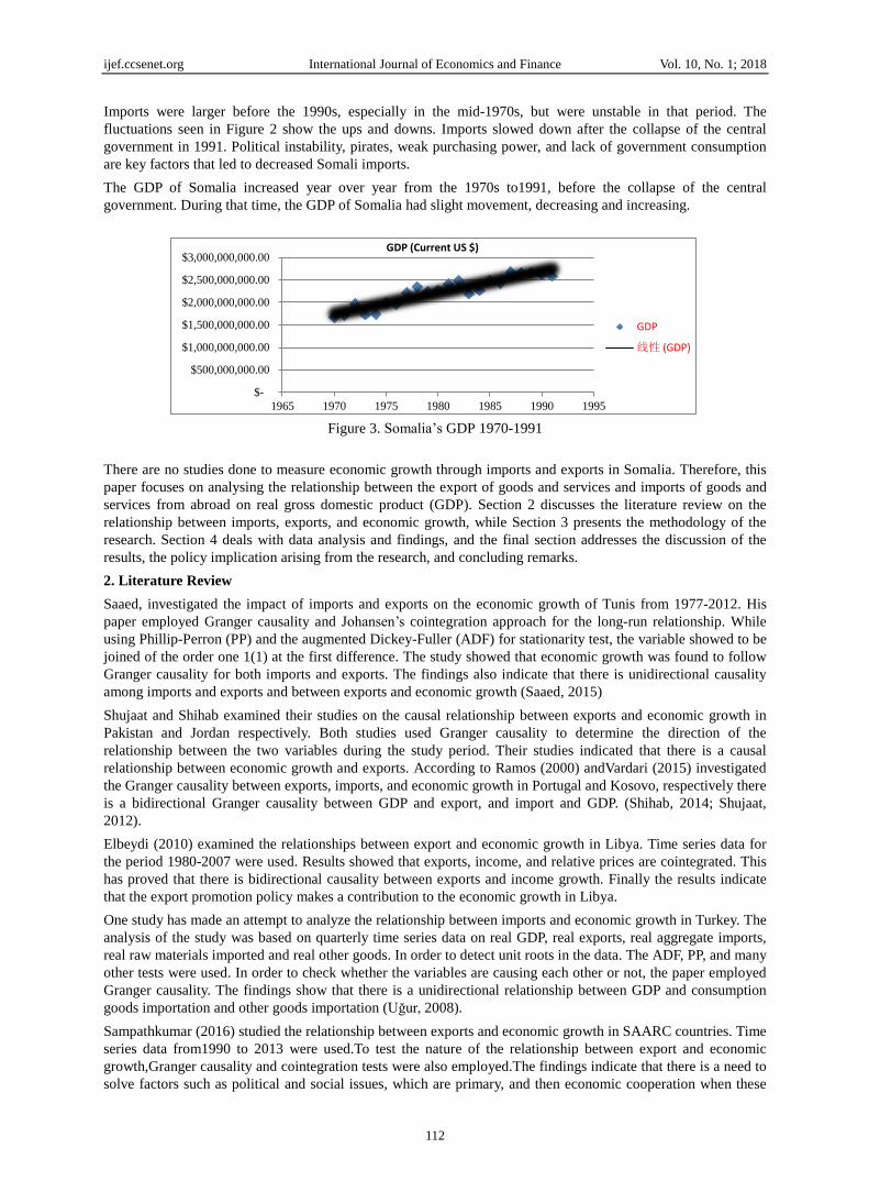
The GDP of Somalia increased year over year from the 1970s to1991, before the collapse of the central

government. During that time, the GDP of Somalia had slight movement, decreasing and increasing.

Figure 3. Somalia’s GDP 1970-1991

There are no studies done to measure economic growth through imports and exports in Somalia. Therefore, this

paper focuses on analysing the relationship between the export of goods and services and imports of goods and

services from abroad on real gross domestic product (GDP). Section 2 discusses the literature review on the

relationship between imports, exports, and economic growth, while Section 3 presents the methodology of the

research. Section 4 deals with data analysis and findings, and the final section addresses the discussion of the

results, the policy implication arising from the research, and concluding remarks.

2. Literature Review

Saaed, investigated the impact of imports and exports on the economic growth of Tunis from 1977-2012. His

paper employed Granger causality and Johansen’s cointegration approach for the long-run relationship. While

using Phillip-Perron (PP) and the augmented Dickey-Fuller (ADF) for stationarity test, the variable showed to be

joined of the order one 1(1) at the first difference. The study showed that economic growth was found to follow

Granger causality for both imports and exports. The findings also indicate that there is unidirectional causality

among imports and exports and between exports and economic growth (Saaed, 2015)

Shujaat and Shihab examined their studies on the causal relationship between exports and economic growth in

Pakistan and Jordan respectively. Both studies used Granger causality to determine the direction of the

relationship between the two variables during the study period. Their studies indicated that there is a causal

relationship between economic growth and exports. According to Ramos (2000) andVardari (2015) investigated

the Granger causality between exports, imports, and economic growth in Portugal and Kosovo, respectively there

is a bidirectional Granger causality between GDP and export, and import and GDP. (Shihab, 2014; Shujaat,

2012).

Elbeydi (2010) examined the relationships between export and economic growth in Libya. Time series data for

the period 1980-2007 were used. Results showed that exports, income, and relative prices are cointegrated. This

has proved that there is bidirectional causality between exports and income growth. Finally the results indicate

that the export promotion policy makes a contribution to the economic growth in Libya.

One study has made an attempt to analyze the relationship between imports and economic growth in Turkey. The

analysis of the study was based on quarterly time series data on real GDP, real exports, real aggregate imports,

real raw materials imported and real other goods. In order to detect unit roots in the data. The ADF, PP, and many

other tests were used. In order to check whether the variables are causing each other or not, the paper employed

Granger causality. The findings show that there is a unidirectional relationship between GDP and consumption

goods importation and other goods importation (Uğur, 2008).

Sampathkumar (2016) studied the relationship between exports and economic growth in SAARC countries. Time

series data from1990 to 2013 were used.To test the nature of the relationship between export and economic

growth,Granger causality and cointegration tests were also employed.The findings indicate that there is a need to

solve factors such as political and social issues, which are primary, and then economic cooperation when these

$-

$500,000,000.00

$1,000,000,000.00

$1,500,000,000.00

$2,000,000,000.00

$2,500,000,000.00

$3,000,000,000.00

1965 1970 1975 1980 1985 1990 1995

GDP (Current US $)

GDP

线性 (GDP)


113

factors are settled.

Ronit (2014) studied the relationship between exports and the economic growth of India. The results show that a

Granger causality test concluded that GDP growth causes export growth, and the impulse response functions

generated also indicate that there are higher reactions of exports over a change in GDP. Kundu (2013)

investigated the export-led growth in seven SAARC countries. The study used panel data analysis, and unit root

and cointegration tests were employed. The paper concluded that there is sufficient evidenceto support the

export-led growth in the extent.

Mehrara (2011) investigated the causal relationship between export growth and economic growth in developing

countries. panel data from 73 countries were used. Granger causlaity and cointegration tests were also used. The

study divided these countries into two groups oil-depedent and non-iol-dependent countries. The results indicate

that there is bidirectional short-run causality between export and GDP growth for non-oil developing

countries,where, for oil countries, there is no short-run causality relationship between exports and economic

growth.

In an open economy, countries are focused on the improvement of the quality of life of their citizens, and quality

of life is an indicator of economic development. Mishra (2011) investigated the dynamic relationship between

exports and economic growth in India. Time series data from 1970-2009 were used vector error correction and

cointegration estimations were applied. The results show that there is a rejection of the export-led growth

strategy in India. Another study on Namibia was carried out by Niishinda, 2013 who examined the relationship

between exports and economic growth in Namibia. Time series data from 1972-2010 were used. To test the

nature of the relationship among the variables, the vector-error correction model (VECM) and Granger causality

tests were applied. The results show that the economic growth of Namibia is dependent on export performance.

3. Methodology

In this study, a multivariate model is employed by using the econometric techniques of the unit root test, the

Johansen test of cointegration, the pairwise Granger causality test, and the VECM model in order to test if there

is a causal relationship between real output growth and the import and export of goods and services, as

mentioned in the introductory section.

3.1 Data and Model Specifications

In this study, a time series analysis is conducted on economic growth, imports, and exports. Data from

1970-1991 used in this study were obtained from the World Bank and the IMF. Then regression analysis is used

to find out the significant impact of imports and exports on economic growth. In this study, E-views version 7

was utilized.

There is a critical assumption that the time series data are stationary or have a unit root in regression analysis.

Broadly speaking, a time series is stationary if its mean and variance are constant over time and the covariance

value between two time periods depends only on the distance between the two periods and not the actual time at

which the covariance is computed (Gujarati, 2012). In this study, the regression model specification is shown

below:

GDPt = β0 +β1IMPt + β2EXPt + µ t

Where GDPt = gross domestic product; IMPt = import of goods and services; EXPt = export of goods and services;

β0 = intercept, β1, β2= slopes of the import and export, respectively; and µ t = stochastic error term of the model.

3.2 Model Diagnostic Assumption Tests

In this study, the model is checked to be free from issues such as heteroscedasticity, serial correlation, and lack of

normality distribution in the error terms. The study uses the appropriate econometric model assumption tests in

order to verify its fitness.

3.3 Unit Root Test

So as to check if the variables of the model have a unit root or not—or if variables are stationary or

non-stationary—the ADF and PP tests will be run.

3.4 Pairwise Granger Causality Test

Usually time does not run backward. That is, if event A happens before event B, then it is possible that A is

causing B. However, it is not possible that B is causing A. In other words, events in the past can cause events to

happen today, but future events cannot. This line of thinking is probably behind the so-called Granger causality

test.


114

In this study, in order to check the direction of causality among the three variables in the model, for instance if

imports cause exports or vice-versa, then the pairwise Granger causality test is used. The question we now ask is:

What is the relationship between GDP, imports, and exports? Does GDP → EXP, or does EXP → GDP, where

the arrow points to the direction of causality?

In this study, the maximum lag length is chosen based on the minimum Akaike information criterion (AIC).The

Granger test involves estimating pairs of regressions.

3.5 Johannsen’s Test of Cointegration and the VECM Model

The long-term association of the variables in the study is required to be checked. Therefore, the researcher applied

the Johansen test of cointegration. On one hand, the VECM model is used if it is found that there is a long-run

relationship among the variables. On the other hand, if there is no long-run relationship among the variables, the

unrestricted VAR model is used in order to verify the long-term and short-term causality of the independent

variables on the dependent variable.

4. Data Analysis and Findings

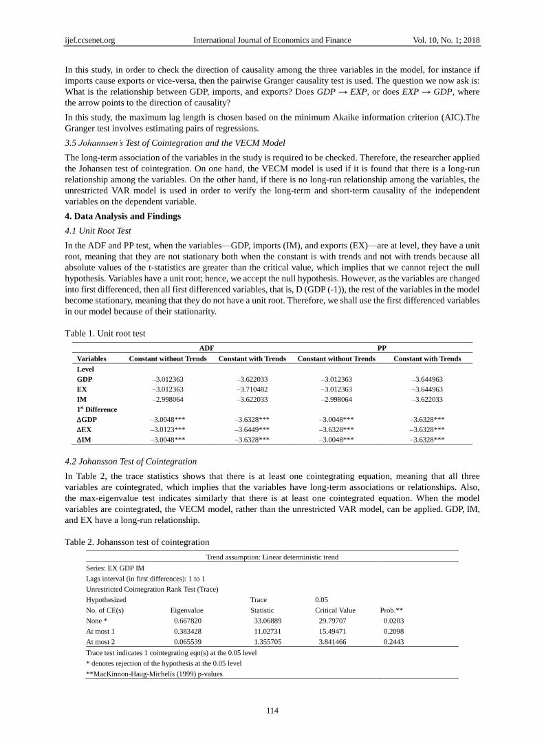
4.1 Unit Root Test

In the ADF and PP test, when the variables—GDP, imports (IM), and exports (EX)—are at level, they have a unit

root, meaning that they are not stationary both when the constant is with trends and not with trends because all

absolute values of the t-statistics are greater than the critical value, which implies that we cannot reject the null

hypothesis. Variables have a unit root; hence, we accept the null hypothesis. However, as the variables are changed

into first differenced, then all first differenced variables, that is, D (GDP (-1)), the rest of the variables in the model

become stationary, meaning that they do not have a unit root. Therefore, we shall use the first differenced variables

in our model because of their stationarity.

Table 1. Unit root test

ADF PP

Variables Constant without Trends Constant with Trends Constant without Trends Constant with Trends

Level

GDP –3.012363 –3.622033 –3.012363 –3.644963

EX –3.012363 –3.710482 –3.012363 –3.644963

IM –2.998064 –3.622033 –2.998064 –3.622033

1st Difference

GDP –3.0048*** –3.6328*** –3.0048*** –3.6328***

EX –3.0123*** –3.6449*** –3.6328*** –3.6328***

IM –3.0048*** –3.6328*** –3.0048*** –3.6328***

4.2 Johansson Test of Cointegration

In Table 2, the trace statistics shows that there is at least one cointegrating equation, meaning that all three

variables are cointegrated, which implies that the variables have long-term associations or relationships. Also,

the max-eigenvalue test indicates similarly that there is at least one cointegrated equation. When the model

variables are cointegrated, the VECM model, rather than the unrestricted VAR model, can be applied. GDP, IM,

and EX have a long-run relationship.

Table 2. Johansson test of cointegration

Trend assumption: Linear deterministic trend

Series: EX GDP IM

Lags interval (in first differences): 1 to 1

Unrestricted Cointegration Rank Test (Trace)

Hypothesized Trace 0.05

No. of CE(s) Eigenvalue Statistic Critical Value Prob.**

None * 0.667820 33.06889 29.79707 0.0203

At most 1 0.383428 11.02731 15.49471 0.2098

At most 2 0.065539 1.355705 3.841466 0.2443

Trace test indicates 1 cointegrating eqn(s) at the 0.05 level

* denotes rejection of the hypothesis at the 0.05 level

**MacKinnon-Haug-Michelis (1999) p-values


115

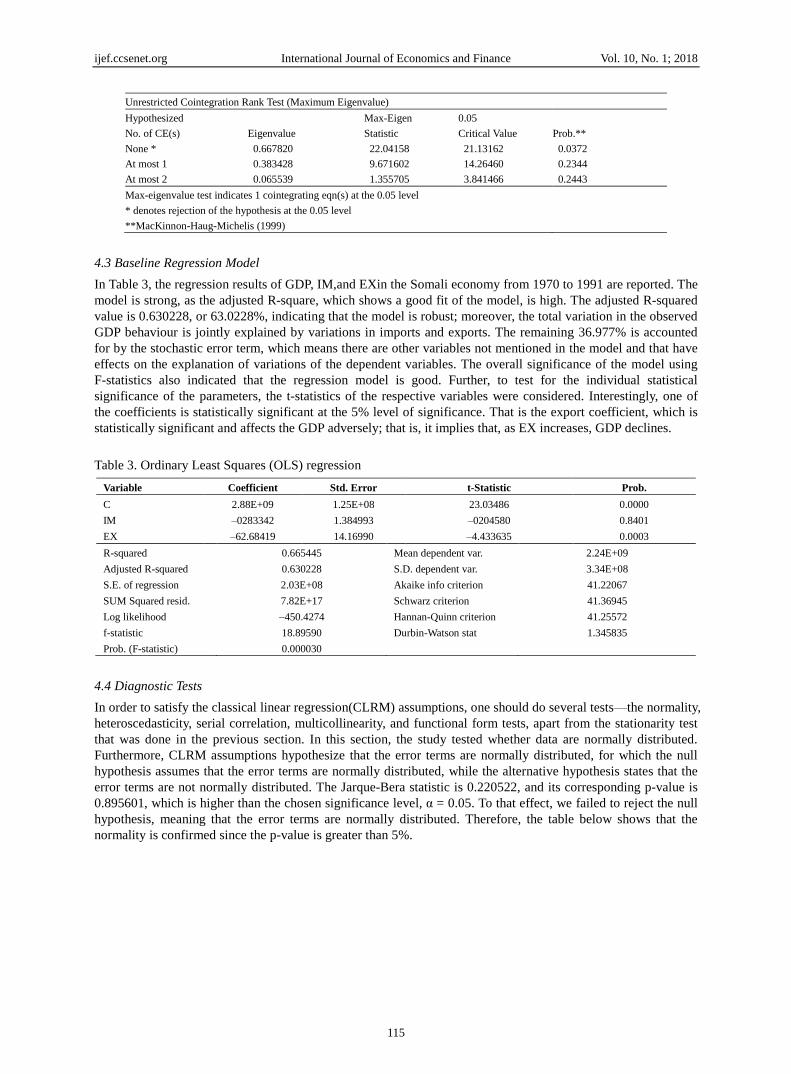
Unrestricted Cointegration Rank Test (Maximum Eigenvalue)

Hypothesized Max-Eigen 0.05

No. of CE(s) Eigenvalue Statistic Critical Value Prob.**

None * 0.667820 22.04158 21.13162 0.0372

At most 1 0.383428 9.671602 14.26460 0.2344

At most 2 0.065539 1.355705 3.841466 0.2443

Max-eigenvalue test indicates 1 cointegrating eqn(s) at the 0.05 level

* denotes rejection of the hypothesis at the 0.05 level

**MacKinnon-Haug-Michelis (1999)

4.3 Baseline Regression Model

In Table 3, the regression results of GDP, IM,and EXin the Somali economy from 1970 to 1991 are reported. The

model is strong, as the adjusted R-square, which shows a good fit of the model, is high. The adjusted R-squared

value is 0.630228, or 63.0228%, indicating that the model is robust; moreover, the total variation in the observed

GDP behaviour is jointly explained by variations in imports and exports. The remaining 36.977% is accounted

for by the stochastic error term, which means there are other variables not mentioned in the model and that have

effects on the explanation of variations of the dependent variables. The overall significance of the model using

F-statistics also indicated that the regression model is good. Further, to test for the individual statistical

significance of the parameters, the t-statistics of the respective variables were considered. Interestingly, one of

the coefficients is statistically significant at the 5% level of significance. That is the export coefficient, which is

statistically significant and affects the GDP adversely; that is, it implies that, as EX increases, GDP declines.

Table 3. Ordinary Least Squares (OLS) regression

Variable Coefficient Std. Error t-Statistic Prob.

C

IM

EX

2.88E+09

–0283342

–62.68419

1.25E+08

1.384993

14.16990

23.03486

–0204580

–4.433635

0.0000

0.8401

0.0003

R-squared

Adjusted R-squared

S.E. of regression

SUM Squared resid.

Log likelihood

f-statistic

Prob. (F-statistic)

0.665445

0.630228

2.03E+08

7.82E+17

–450.4274

18.89590

0.000030

Mean dependent var.

S.D. dependent var.

Akaike info criterion

Schwarz criterion

Hannan-Quinn criterion

Durbin-Watson stat

2.24E+09

3.34E+08

41.22067

41.36945

41.25572

1.345835

4.4 Diagnostic Tests

In order to satisfy the classical linear regression(CLRM) assumptions, one should do several tests—the normality,

heteroscedasticity, serial correlation, multicollinearity, and functional form tests, apart from the stationarity test

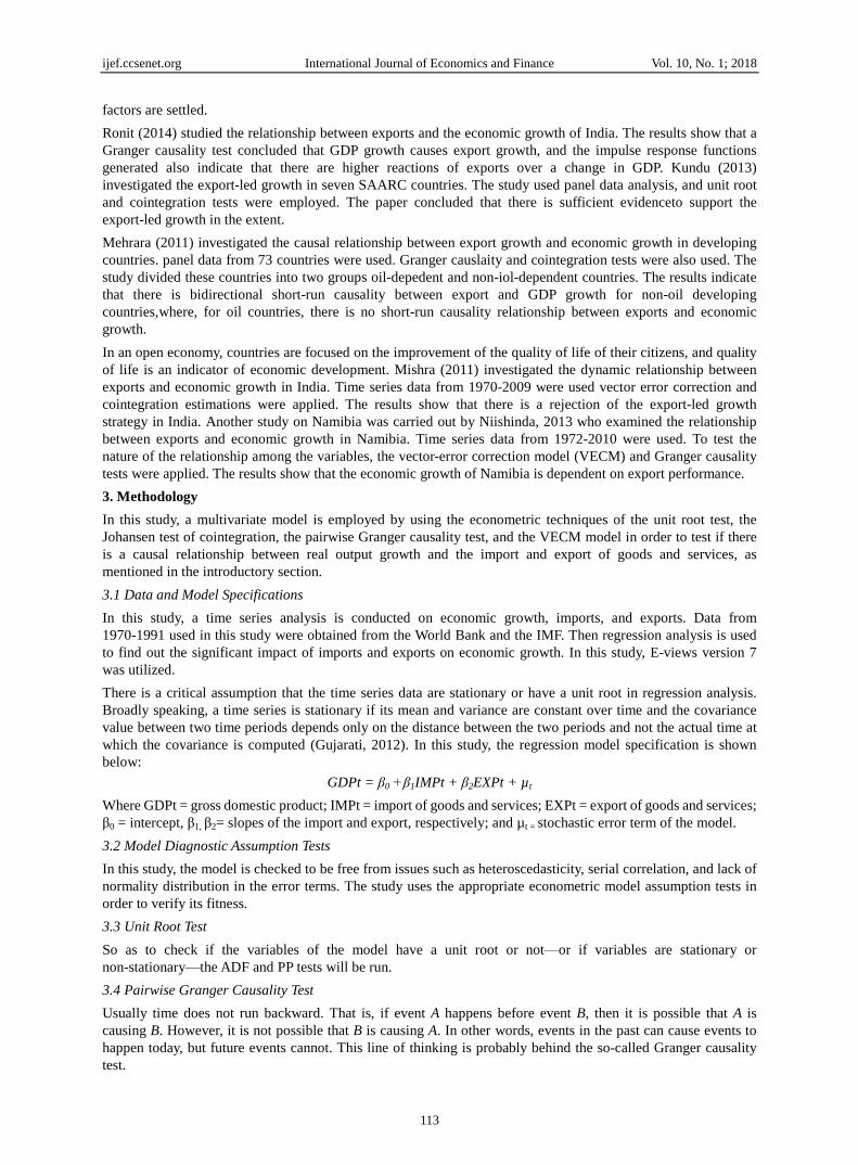
that was done in the previous section. In this section, the study tested whether data are normally distributed.

Furthermore, CLRM assumptions hypothesize that the error terms are normally distributed, for which the null

hypothesis assumes that the error terms are normally distributed, while the alternative hypothesis states that the

error terms are not normally distributed. The Jarque-Bera statistic is 0.220522, and its corresponding p-value is

0.895601, which is higher than the chosen significance level, α = 0.05. To that effect, we failed to reject the null

hypothesis, meaning that the error terms are normally distributed. Therefore, the table below shows that the

normality is confirmed since the p-value is greater than 5%.


116

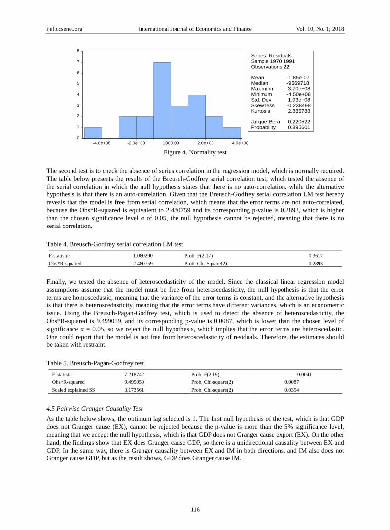
Figure 4. Normality test

The second test is to check the absence of series correlation in the regression model, which is normally required.

The table below presents the results of the Breusch-Godfrey serial correlation test, which tested the absence of

the serial correlation in which the null hypothesis states that there is no auto-correlation, while the alternative

hypothesis is that there is an auto-correlation. Given that the Breusch-Godfrey serial correlation LM test hereby

reveals that the model is free from serial correlation, which means that the error terms are not auto-correlated,

because the Obs*R-squared is equivalent to 2.480759 and its corresponding p-value is 0.2893, which is higher

than the chosen significance level α of 0.05, the null hypothesis cannot be rejected, meaning that there is no

serial correlation.

Table 4. Breusch-Godfrey serial correlation LM test

F-statistic 1.080290 Prob. F(2,17) 0.3617

Obs*R-squared 2.480759 Prob. Chi-Square(2) 0.2893

Finally, we tested the absence of heteroscedasticity of the model. Since the classical linear regression model

assumptions assume that the model must be free from heteroscedasticity, the null hypothesis is that the error

terms are homoscedastic, meaning that the variance of the error terms is constant, and the alternative hypothesis

is that there is heteroscedasticity, meaning that the error terms have different variances, which is an econometric

issue. Using the Breusch-Pagan-Godfrey test, which is used to detect the absence of heteroscedasticity, the

Obs*R-squared is 9.499059, and its corresponding p-value is 0.0087, which is lower than the chosen level of

significance α = 0.05, so we reject the null hypothesis, which implies that the error terms are heteroscedastic.

One could report that the model is not free from heteroscedasticity of residuals. Therefore, the estimates should

be taken with restraint.

Table 5. Breusch-Pagan-Godfrey test

F-statistic

Obs*R-squared

Scaled explained SS

7.218742

9.499059

3.173561

Prob. F(2,19)

Prob. Chi-square(2)

Prob. Chi-square(2)

0.0041

0.0087

0.0354

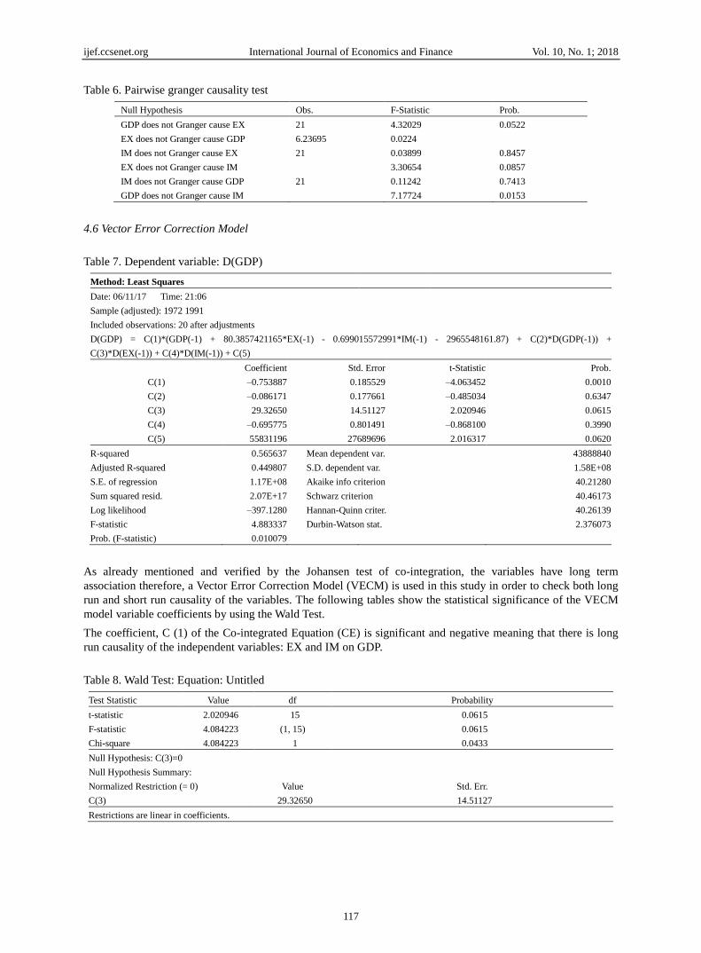
4.5 Pairwise Granger Causality Test

As the table below shows, the optimum lag selected is 1. The first null hypothesis of the test, which is that GDP

does not Granger cause (EX), cannot be rejected because the p-value is more than the 5% significance level,

meaning that we accept the null hypothesis, which is that GDP does not Granger cause export (EX). On the other

hand, the findings show that EX does Granger cause GDP, so there is a unidirectional causality between EX and

GDP. In the same way, there is Granger causality between EX and IM in both directions, and IM also does not

Granger cause GDP, but as the result shows, GDP does Granger cause IM.

0

1

2

3

4

5

6

7

8

-4.0e+08 -2.0e+08 1000.00 2.0e+08 4.0e+08

Series: ResidualsSample 1970 1991Observations 22

Mean -1.85e-07Median -9569718.Maximum 3.70e+08Minimum -4.50e+08Std. Dev. 1.93e+08Skewness -0.238498Kurtosis 2.885788

Jarque-Bera 0.220522Probability 0.895601


117

Table 6. Pairwise granger causality test

Null Hypothesis Obs. F-Statistic Prob.

GDP does not Granger cause EX

EX does not Granger cause GDP

21

6.23695

4.32029

0.0224

0.0522

IM does not Granger cause EX

EX does not Granger cause IM

21

0.03899

3.30654

0.8457

0.0857

IM does not Granger cause GDP

GDP does not Granger cause IM

21

0.11242

7.17724

0.7413

0.0153

4.6 Vector Error Correction Model

Table 7. Dependent variable: D(GDP)

Method: Least Squares

Date: 06/11/17 Time: 21:06

Sample (adjusted): 1972 1991

Included observations: 20 after adjustments

D(GDP) = C(1)*(GDP(-1) + 80.3857421165*EX(-1) - 0.699015572991*IM(-1) - 2965548161.87) + C(2)*D(GDP(-1)) +

C(3)*D(EX(-1)) + C(4)*D(IM(-1)) + C(5)

Coefficient Std. Error t-Statistic Prob.

C(1) –0.753887 0.185529 –4.063452 0.0010

C(2) –0.086171 0.177661 –0.485034 0.6347

C(3) 29.32650 14.51127 2.020946 0.0615

C(4) –0.695775 0.801491 –0.868100 0.3990

C(5) 55831196 27689696 2.016317 0.0620

R-squared 0.565637 Mean dependent var. 43888840

Adjusted R-squared 0.449807 S.D. dependent var. 1.58E+08

S.E. of regression 1.17E+08 Akaike info criterion 40.21280

Sum squared resid. 2.07E+17 Schwarz criterion 40.46173

Log likelihood –397.1280 Hannan-Quinn criter. 40.26139

F-statistic 4.883337 Durbin-Watson stat. 2.376073

Prob. (F-statistic) 0.010079

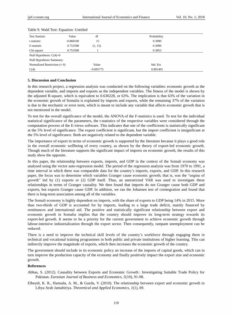
As already mentioned and verified by the Johansen test of co-integration, the variables have long term

association therefore, a Vector Error Correction Model (VECM) is used in this study in order to check both long

run and short run causality of the variables. The following tables show the statistical significance of the VECM

model variable coefficients by using the Wald Test.

The coefficient, C (1) of the Co-integrated Equation (CE) is significant and negative meaning that there is long

run causality of the independent variables: EX and IM on GDP.

Table 8. Wald Test: Equation: Untitled

Test Statistic Value df Probability

t-statistic 2.020946 15 0.0615

F-statistic 4.084223 (1, 15) 0.0615

Chi-square 4.084223 1 0.0433

Null Hypothesis: C(3)=0

Null Hypothesis Summary:

Normalized Restriction (= 0) Value Std. Err.

C(3) 29.32650 14.51127

Restrictions are linear in coefficients.


118

Table 9. Wald Test: Equation: Untitled

Test Statistic Value df Probability

t-statistic –0.868100 15 0.3990

F-statistic 0.753598 (1, 15) 0.3990

Chi-square 0.753598 1 0.3853

Null Hypothesis: C(4)=0

Null Hypothesis Summary:

Normalized Restriction (= 0) Value Std. Err.

C(4) –0.695775 0.801491

5. Discussion and Conclusion

In this research project, a regression analysis was conducted on the following variables: economic growth as the

dependent variable, and imports and exports as the independent variables. The fitness of the model is shown by

the adjusted R-square, which is equivalent to 0.630228, or 63%. The implication is that 63% of the variation in

the economic growth of Somalia is explained by imports and exports, while the remaining 37% of the variation

is due to the stochastic or error term, which is meant to include any variable that affects economic growth that is

not mentioned in the model.

To test for the overall significance of the model, the ANOVA of the F-statistics is used. To test for the individual

statistical significance of the parameters, the t-statistics of the respective variables were considered through the

computation process of the E-views software. This indicates that one of the coefficients is statistically significant

at the 5% level of significance. The export coefficient is significant, but the import coefficient is insignificant at

the 5% level of significance. Both are negatively related to the dependent variable.

The importance of export in terms of economic growth is supported by the literature because it plays a good role

in the overall economic wellbeing of every country, as shown by the theory of export-led economic growth.

Though much of the literature supports the significant impact of imports on economic growth, the results of this

study show the opposite.

In this paper, the relationship between exports, imports, and GDP in the context of the Somali economy was

analysed using the vector auto-regression model. The period of the regression analysis was from 1970 to 1991, a

time interval in which there was comparable data for the country’s imports, exports, and GDP. In this research

paper, the focus was to determine which variables Granger cause economic growth; that is, was the ―engine of

growth‖ led by (1) exports or (2) GDP itself. Thus, an unrestricted VAR was used to investigate these

relationships in terms of Granger causality. We then found that imports do not Granger cause both GDP and

exports, but exports Granger cause GDP. In addition, we ran the Johansen test of cointegration and found that

there is long-term association among all of the variables.

The Somali economy is highly dependent on imports, with the share of exports to GDP being 14% in 2015. More

than two-thirds of GDP is accounted for by imports, leading to a large trade deficit, mainly financed by

remittances and international aid. The positive and statistically significant relationship between export and

economic growth in Somalia implies that the country should improve its long-term strategy towards its

export-led growth. It seems to be a priority for the current government to achieve economic growth through

labour-intensive industrialization through the export sector. Then consequently, rampant unemployment can be

reduced.

There is a need to improve the technical skill levels of the country’s workforce through engaging them in

technical and vocational training programmes in both public and private institutions of higher learning. This can

indirectly improve the magnitude of exports, which then increases the economic growth of the country.

The government should include in its economic policy an increase of the imports of capital goods, which can in

turn improve the production capacity of the economy and finally positively impact the export size and economic

growth.

References

Abbas, S. (2012). Causality between Exports and Economic Growth : Investigating Suitable Trade Policy for

Pakistan. Eurasian Journal of Business and Economics, 5(10), 91-98.

Elbeydi, K. R., Hamuda, A. M., & Gazda, V. (2010). The relationship between export and economic growth in

Libya Arab Jamahiriya. Theoretical and Applied Economics, 1(1), 69.


119

Kundu, A. (2013). Bi-directional relationships between exports and growth: A panel data approach. Journal of

Economics and Development Studies, 1(1), 10-23.

Luan, V. (2015). Relationship between Import-Exports and Economic Growth: The Kosova Case Study. Revista

Shkencore Regjionale (REFORMA), 3, 262-269.

Mehrara, M., & Firouzjaee, B. A. (2011). Granger causality relationship between export growth and GDP growth

in developing countries: Panel cointegration approach. International Journal of Humanities and Social

Science, 1(16), 223-231.

Mishra, P. K. (2011). The dynamics of relationship between exports and economic growth in India. International

Journal of Economic Sciences and Applied Research, 4(2), 53-70

Niishinda, E. (2013). Testing the Long-run Relationship between Export and Economic Growth: Evidence from

Namibia. Journal of Emerging Issues in Economics, Finance and Banking (JEIEFB), 1(5), 244-261.

Ramos, F. F. R. (2001). Exports, imports, and economic growth in Portugal: Evidence from causality and

cointegration analysis. Economic Modelling, 18(4), 613-623.

Ronit, M., & Divya, P. (2014). The relationship between the growth of exports and growth of gross domestic

product in India. International Journal of Business and Economics Research, 3(3), 135-139.

https://doi.org/10.11648/j.ijber.20140303.13

Saaed, A. A. J., & Hussain, M. A. (2015). Impact of exports and imports on economic growth: Evidence from

Tunisia. Journal of Emerging Trends in Economics and Management Sciences, 6(1), 13.

Sampathkumar, T., & Rajeshkumar, S. (2016). Causal Relationship between Export and Economic Growth:

Evidence from SAARC Countries. IOSR Journal of Economics and Finance Ver. I, 7(3), 2321-5933.

https://doi.org/10.9790/5933-0703013239

Shihab, R. A., Soufan, T., & Abdul-khaliq, S. (2014). The Causal Relationship between Exports and Economic.

Global Journal of Management and Business Research, 14(3), 1-7.

Uğur, A. (2008). Import and economic growth in Turkey: Evidence from multivariate VAR analysis. Journal of

Economics and Business, 11(1-2), 54-75.

Copyrights

Copyright for this article is retained by the author(s), with first publication rights granted to the journal.

This is an open-access article distributed under the terms and conditions of the Creative Commons Attribution

license (http://creativecommons.org/licenses/by/4.0/).

Documents

The Impact of Imports and Exports Performance on the